Overview of the RIO-SFE program and Remote Sensing with Landsat 8

and Sentinel 2Curtiss O. Davis, Nicholas

Tufillaro and Jasmine Nahorniak

College of Earth, Ocean and Atmospheric Sciences,Oregon State University, Corvallis, OR, USA 97331cdavis@coas.oregonstate.edu

Impacts of Population Growth on the San Francisco Bay and Delta Ecosystem (SFE)

The goal of this NASA Interdisciplinary Science project is to putin place an approach and modeling framework for the scientificbasis of an ecosystem approach to the stewardship of the SFEincluding freshwater and marine resources within the SFE andadjacent ocean ecosystems. Our SFE project combines fourcomponents:

(1) Satellite observations(MERIS, HICO, Landsat, Sentinel 2 and in the future OLCI)

(2) In situ observations (nutrients, phytoplankton, suspended sediments, CDOM andoptical properties)

(3) CoSiNE bio-optical model of SFE integrated with the SCHISM hydrological model of SFE

(4) Coordination with Stakeholders

Three year effort to establish an integrated approach using remote sensing, in situ data and modeling to study SFE.

RIO-SFE ProjectRemote/In situ Observing - San Francisco Bay and Estuary

CoSiNE ecological model

(Fei Chai, U. Maine)

SCHISMSemi-implicit Cross-scale Hydroscience Integrated System

Model(Yi Chao, RSI)

Resultsmerging data and

models to understand SFE Remote Sensing

(Curt Davis, OSU)

Field Observations(RTC, NRL and OSU)

Results and discussions with SFE Stakeholders: November 14, 2016

Sacramento, CA

RIO-SFE Remote Sensing

MERIS2002-2012, 10 year time series300 m GSD, 16 ocean bands, high

SNRHICOSept 2009 – Sept 2014 90 m GSD, high SNRhyperspectral (400 – 900 nm at 5.7

nm resolution)collects scenes on demand

Landsat-OLI 30 m GSD, 16 day revisit, land

bands, moderate SNR, 15 m panchromatic band

Sentinel 220 m GSD, additional bands for

vegetation

MERIS FR image from 23 June 2011

RGB image Algal-2 chlorophyll product showing values ranging from 2 (yellow) to 20 (pink) mg/m3 .

MERIS data are available over a 10 year period (2002 – 2012) MERIS provides 300 m GSD, 16 ocean bands, and high SNR

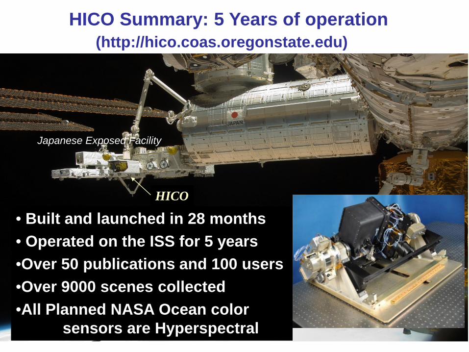
HICO Summary: 5 Years of operation(http://hico.coas.oregonstate.edu)

Japanese Exposed Facility

HICO

• Built and launched in 28 months• Operated on the ISS for 5 years•Over 50 publications and 100 users•Over 9000 scenes collected•All Planned NASA Ocean color

sensors are Hyperspectral

HICO image from February 19, 2014

Remote sensing reflectance spectra for:(1) Suisun Bay (very high

sediments),(2) San Pablo Bay (high

sediments), and(3) offshore showing

outflow from the Bay.

Suisun Bay

San Pablo Bay

offshore

Having the full spectra allows separation of the

sediment and chlorophyll signals and in some

cases the identification of bloom species.

Landsat-OLI image from 28 May 2014

Landsat provides 30 m GSD, 16 day revisit, land bands and moderate SNR.

15 m Panchromatic band for image sharpening

Especially good for the delta and adjacent land areas.

Challenge to make good ocean products due to limited band set and low SNR for ocean scenes.

Landsat 8 OLI CharacteristicsLandsat 8OperationalLand Imager(OLI)

LaunchedFebruary 11, 2013

Bands Wavelength(micrometers)

Resolution(meters)

Band 1 - Coastal aerosol 0.43 - 0.45 30

Band 2 - Blue 0.45 - 0.51 30Band 3 - Green 0.53 - 0.59 30Band 4 - Red 0.64 - 0.67 30Band 5 - Near Infrared (NIR) 0.85 - 0.88 30

Band 6 - SWIR 1 1.57 - 1.65 30Band 7 - SWIR 2 2.11 - 2.29 30Band 8 -Panchromatic 0.50 - 0.68 15

Band 9 - Cirrus 1.36 - 1.38 30Landsat bands are optimized for land products and

here we adapt them for coastal ocean products.

Landsat 8-OLI Processing MethodsLandsat-8 OLI San Francisco Bay Atmospheric correction uses an iterative SWIR method optimized for highly turbid waters (Vanhellemont & Ruddick 2014) using the ‘Acolite’ processor created by Vanhellemont and coworkers.

Total Suspended Sediment (TSS) maps (Nechad, Ruddick, and Park 2010) typically show an increase of turbidity in the lower Sacramento River and North San Pablo Bay. Product maps like these are used for the calibration and validation of the SFE model. The product maps are ‘regionally tuned’ using in situ observations.

Images are sharpened using the 15 m Panchromatic band.

Turbidity 22 April 2015

Turbidity 08 May 2015

Suisun Bay Franks

TractSan Pablo Bay

Sacramento River

San JoaquinRiver

SPM Maps from L-8 OLI data

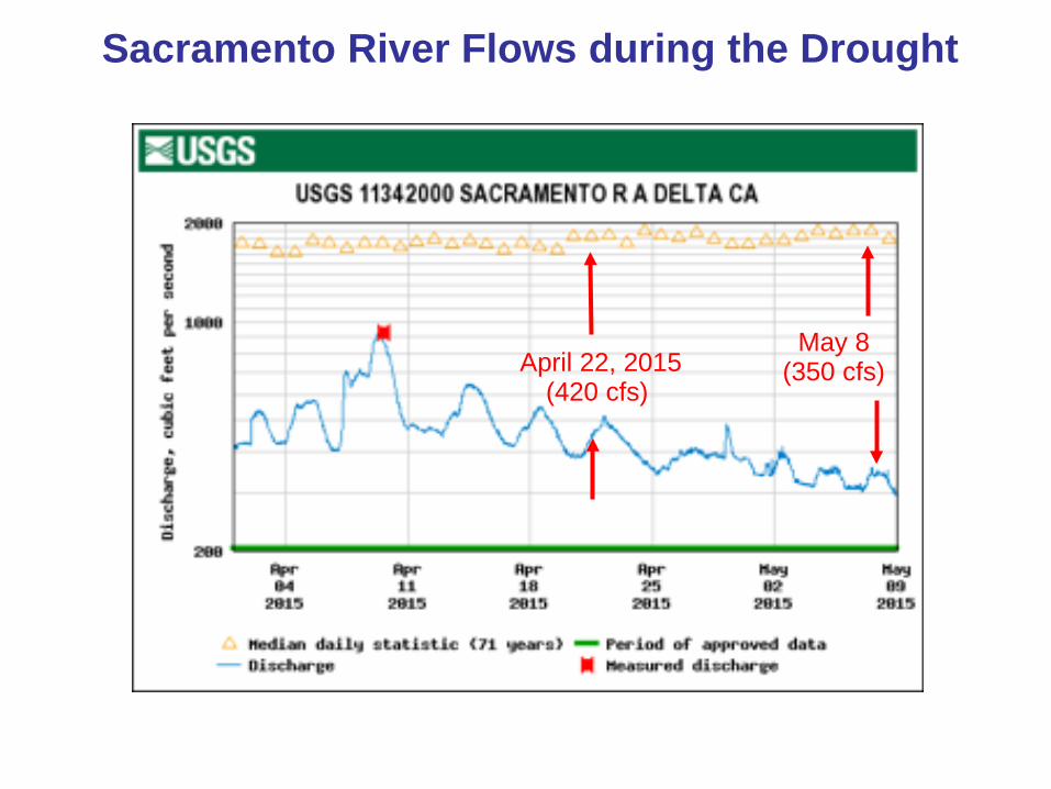
“the miracle in march”Sacramento River Flows during the Drought

April 22, 2015(420 cfs)

May 8(350 cfs)

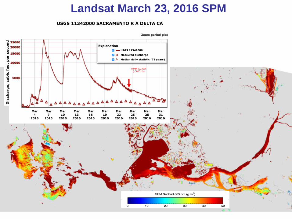
March 23, 2016(~3000 cfs)

Landsat March 23, 2016 SPM

22 April 2015 8 May 2015Suisun Bay to Franks TractLandsat 8 OLI 8 May 2015SWIR Atmospheric Correctionfor highly turbid waters (Vanhellemont and Ruddick 2014) Pan Enhancement (15m) False River West False River West

Beginning of ‘Salinity Barrier’

False River West

Suisun Bay

Franks Tract

Following the Franks Tract Salinity Barrier

LS-8 OLI Franks Tract Aug 12, 2015

Macro Algae filling Franks Tract

Stuckenia pectinataSago pondweed, native, freshwater to salinity ~14

Potamogeton crispus ,curly (or curled-leaf) pondweed, non-native, freshwater

ASlaughter, photo

Sept 4. 2015 Franks Tract ship samples

2015

2014

Frank’s Tract Vegetation classification

Increase in SAV cover and density

Decrease in water hyacinth

ESA Annual Meeting 2016: Airborne Remote Sensing for 21st Century Ecology, Susan Ustin, U.C. Davis

-1 to -0.3-0.3 to -0.1-0.1 to 00 to 0.10.1 to 0.20.2 to 0.30.3 to 0.40.4 to 0.50.5 to 0.60.6 to 0.70.7 to 1

ESA Annual Meeting 2016: Airborne Remote Sensing for 21st Century Ecology, Susan Ustin, U.C. Davis

SAV Mat density from Landsat

November 2014 Frank's Tract: SAV mat density September 2015

0 0.75 1.5 3 .... c=== ........ Km

Sentinel 2 Bands — Even Better for Water

Spatial 10 Meters

Spectral -Maximum Chlorophyll Index

Suisun Slough Merges into Suisun BaySentinel-2: 30 March 2016

May 2016 Bloom following March flood

0

20

40

60

80

0

0.1

0.2

0.3

Left. Landsat image overlain with USGS (B. Bergamaschi) measured underway chlorophyll fluorescence from May 6, 2016. Inset May 15, 2016 Sentinel 2 image of the

phytoplankton bloom (Gower et al. 2005 MCI algorithm). Right. SFE May 19 Cruise data for chlorophyll and f ratio (nitrate uptake rate/ (nitrate uptake rate + ammonium

uptake rate) showing how the bloom forms when the phytoplankton are able to take up nitrate. Red arrows indicates the location of the peak bloom.

15 May Sentinel-2Chlorophyll Estimate using MOSES3BRed-edge algorithm (S2A only) to derive chlorophyll a concentrationfrom the red band chlorophyll a absorption.Moses, W.J., Gitelson, A.A., Berdnikov, S., Saprygin, V., Povazhnyi, V., 2012. Operational MERIS basedNIR-red algorithms for estimating chlorophyll-a concentrations in coastal waters—TheAzov Sea case study. Remote Sens. Environ. 121, 118–124.

.., .

• .'

UIO IO.CIO

, . ·­...

. '•

. . .

Progress and PlansComplete processing and analysis of cruise data.

Publications on time series of data and May 2016 bloom.Use MERIS 10 year time series to validate model results.Hyperspectral imaging very valuable to distinguish and

quantify the diversity of coastal blooms (HICO examples)Land sensors can be very useful in the near coastal ocean (Landsat-8 OLI and Sentinel 2A) When Sentinel 2B is operational there will be 5 day repeat coverage. Continue routine monitoring of SFE.Collaborate on a publication on Franks TrackAll data available through NASA SEA-BASS data system

Coordinated team efforts are needed to deal with the complexity of SFE. High resolution remote sensing data

essential to track blooms and other features.