parameter estimation and structural model updating using ... · 2 outline 1. introduction 2....

Rome,

Sep

tembe

r 21

-25,

200

9, S

ICON F

C

Parameter Estimation and Structural Model Updating Using Modal Methods

in the Presence of Nonlinearity

Jean-Claude Golinval

University of Liege, Belgium

Department of Aerospace and Mechanical EngineeringChemin des Chevreuils, 1 Bât. B 52B-4000 Liège (Belgium) E-mail : [email protected]

SICON Final Conference

2Outline

1. Introduction

2. Theoretical Modal Analysis of Nonlinear Systems

3. Nonlinear Experimental Modal Analysis

4. Model Parameter Estimation Techniques

5. Concluding Remarks

3

Design of engineering structures relies on

• Numerical predictions modal analysis (FEM)

• Dynamic testing experimental modal analysis (EMA)

In the case of linear structures, the techniques available for EMA are mature e.g.

• Eigensystem realization algorithm

• Stochastic subspace identification

• Polyreference least-squares complex exponentials frequency domain

• etc

Introduction

4Introduction

Nonlinearity in Engineering Applications

hardening nonlinearities in engine-to-pylon connections

fluid-structure interactionbacklash and friction in

control surfaces and joints

composite materials

Many works are reported in the literature on dynamic testing andidentification of nonlinear systems but very few address nonlinear phenomena during modal survey tests.

5

Aim of this presentation

• To extend experimental modal analysis to a practical analogue using the nonlinear normal mode (NNM) theory.

• Validate mathematical models of non-linear structures against experimental data.

Introduction

Why?

• NNMs offer a solid and rigorous mathematical tool.

• They have a clear conceptual relation to the classical LNMs.

• They are capable of handling strong structural nonlinearity.

6Outline

1. Introduction


• Nonlinear Normal Modes (NNMs)

• Numerical Computation of NNMs

• Frequency-Energy Plot




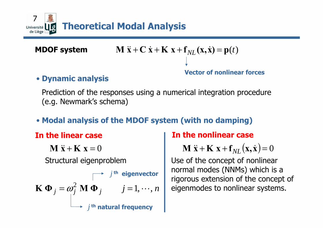
7Theoretical Modal Analysis

• Modal analysis of the MDOF system (with no damping)

• Dynamic analysis

Prediction of the responses using a numerical integration procedure (e.g. Newmark’s schema)

MDOF system

In the nonlinear case

)(tNL p)x(x,fxKxCxM =+++ &&&&

Vector of nonlinear forces

In the linear case

0=+ xKxM && ( ) 0=++ xx,fxKxM &&& NL

j th eigenvector

Structural eigenproblem

njjjj ,,12 L== ΦMΦK ω

j th natural frequency

Use of the concept of nonlinear normal modes (NNMs) which is a rigorous extension of the concept of eigenmodes to nonlinear systems.

8Nonlinear Normal Modes

Definitions

Two definitions of an NNM in the literature:

1. Targeting a straightforward nonlinear extension of the linear normal mode (LNM) concept, Rosenberg defined an NNM motion as a vibration in unison of the system (i.e., a synchronous periodic oscillation).

2. To provide an extension of the NNM concept to damped systems, Shaw and Pierre defined an NNM as a two-dimensional invariant manifold in phase space. Such a manifold is invariant under the flow (i.e., orbits that start out in the manifold remain in it for all time), which generalizes the invariance property of LNMsto nonlinear systems.

In the present study, an NNM motion is defined as a (non-necessarily synchronous) periodic motion of the undamped mechanical system

this extended definition is particularly attractive when targeting a numerical computation of the NNMs.

9

( )( ) 02

05.02

122

31211

=−+=+−+

xxxxxxx

&&

&&

Illustrative example: 2 DOF-system with a cubic stiffness

Nonlinear Normal Modes

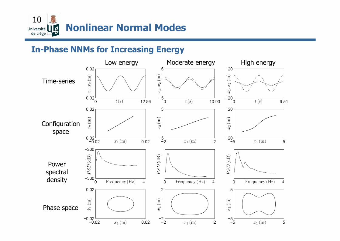
10

In-Phase NNMs for Increasing Energy

Time-series

Configuration space

Phase space

Power spectral density

Low energy Moderate energy High energy

Nonlinear Normal Modes

11

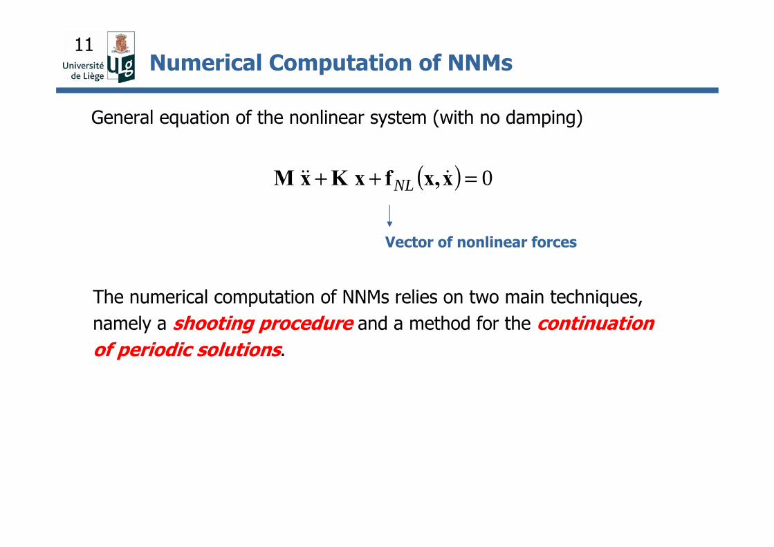
( ) 0=++ xx,fxKxM &&& NL

The numerical computation of NNMs relies on two main techniques, namely a shooting procedure and a method for the continuation of periodic solutions.

Numerical Computation of NNMs

General equation of the nonlinear system (with no damping)


12

• Shooting method

The shooting method consists in finding, in an iterative way, the initial conditions and the period T inducing an isolated periodic motion (i.e., an NNM motion) of the conservative system.

( ) ( )0,00xx &

=tNumericalintegration

( ) ( )TTTtxx &,

=

Newton-Raphson

( ) ( )0,0 xx &


13

• Pseudo-arclength continuation methodIn

itial

con

ditio

ns

Pseudo-arclength continuation method:

predictor step tangent to the branch

NNM branch

Period T


corrector step perpendicular to the predictor step (shooting)

14Frequency-Energy Plot (FEP)

Backbone of the FEP

Modal curves

15Outline

1. Introduction



• Phase Separation Methods

- Proper Orthogonal Decomposition

• Phase Resonance Methods

- Nonlinear Normal Mode Testing



16Experimental Modal Analysis (EMA)

EMA for linear systems is now mature and widely used in structural engineering well established techniques [1], [2].

Finite Element Model Response Measurements

Theoretical Approach Experimental Approach

Eigenvalue problem

0=+ xKxM &&

jjj ΦMΦK 2ω=

Natural frequencies (ωj2)

Mode shapes (Φj)

Time series

Identification methods

Time

Acc

(m

/s2)

Linear systems

17Experimental Modal Analysis (EMA)

EMA for nonlinear systems is still a challenge.

Nonlinear systems

Finite Element Model Response Measurements

Theoretical Approach Experimental Approach

Numerical NNM computation

NNM frequenciesNNM modal curves

Time series

Experimental NNM extraction

( ) 0=++ xx,fxKxM &&& NL

Time

Acc

(m

/s2)

18

There are two main techniques for EMA.

1. Phase separation methods

Several modes are excited at once using either broadband excitation (e.g., hammer impact and random excitation) or swept-sine excitation in the frequency range of interest.

in the nonlinear case, extraction of individual NNMs is not possible generally, because modal superposition is no longer valid.

use of the proper orthogonal decomposition (POD) method to extract features from the time series .

Experimental Modal Analysis (EMA)

Remark

• All structures encountered in practice are nonlinear to some degree.

• If a nonlinear structure is excited with a broadband excitation signal (e.g. random force), then the results will appear linear experimental modal analysis will lead to an updated linearized model !

19

Instrumented structure

⎥⎥⎥

⎦

⎤

⎢⎢⎢

⎣

⎡=

)()(

)()(

1

111

NMM

N

txtx

txtx

L

MOM

L

XM

measurementco-ordinates

N snapshots

[ ])()( 1 Ntt xxX K=

Ω

1xix

Mx

Proper Orthogonal Decomposition (POD)

is the observation matrix

20

The M x M correlation matrix R is built

T

MXXR 1=

The eigenvalue problem is solved

uuR λ=

Eigenvectors of XXT (POMs)

Eigenvalues (POVs)


21

⎥⎥⎥

⎦

⎤

⎢⎢⎢

⎣

⎡=

)()(

)()(

1

111

NMM

N

NxM

txtx

txtx

L

MOM

L

X

M measurement co-ordinates

N time samples

Computation of the POMs using SVD

Using SVD

TVUX NNNMMMNM ×××× Σ=

Eigenvectors of XXT (POM)

)POV()( ≡iidiag λλ


Ω

1xix

Mx

22

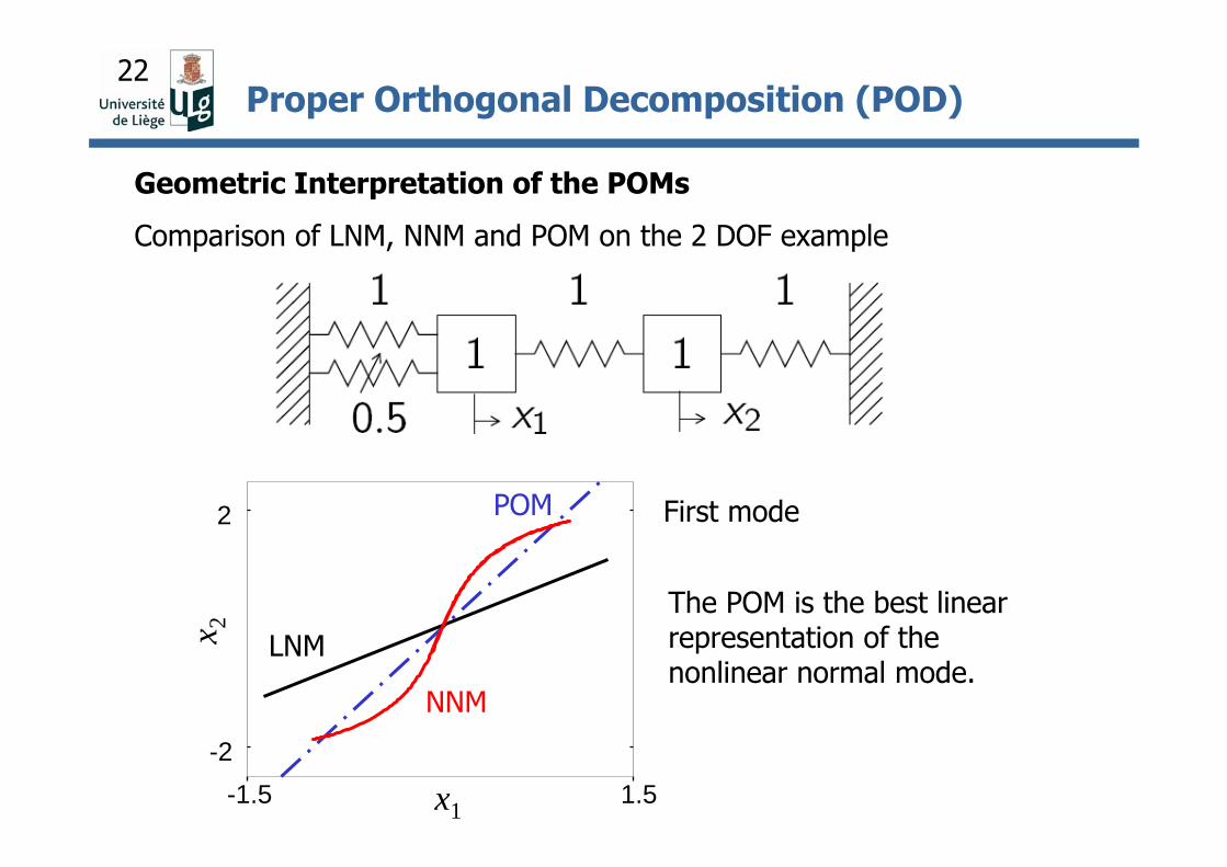
Geometric Interpretation of the POMs

Comparison of LNM, NNM and POM on the 2 DOF example

x1

x 2

-1.5 1.5-2

2

NNM

First mode

LNM

POM

The POM is the best linear representation of the nonlinear normal mode.


23

Nonlinear Systems

Statistical approach

Proper Orthogonal Decomposition :

Response :

Key idea: Application of the POD to Features Extraction

Linear Systems

Deterministic approach

Eigenvalue problem :

Response :

)(tNL p)x(x,fxKxCxM =+++ &&&&)(tpxKxCxM =++ &&&

0ΦMK =− )( 2ω

∑=

=n

iii tt

1)()()( Φx η

TVUX Σ=

∑=

=n

jjj tat

1)()()( ux

Spatial information

Natural frequencies

)sin()cos( tBtA iiiii ωωη +=

Time information

Instantaneous frequencies

Spatial information


24

2. Phase resonance methods (Normal mode testing)

One of the normal mode at a time is excited using multi-point sine excitation at the corresponding natural frequency. The modes areidentified one by one.

can be extended to nonlinear structures according to the invariance property of NNMs:

« If the motion is initiated on one specific NNM, the remaining NNMs remain quiescent for all time. »

Experimental Modal Analysis (EMA)

Remark• Expensive and difficult.• Extremely accurate mode shapes a way to identify NNMs

(but still a research topic).

25

Fundamental properties

1. Forced responses of nonlinear systems at resonance occur in the neighborhood of NNMs [3].

2. According to the invariance property, motions that start out in the NNM manifold remain in it for all time [4].

3. The effect of weak to moderate damping on the transient dynamicsis purely parasitic. The free damped dynamics closely follows the NNM of the underlying undamped system [5, 6, 7]

Nonlinear EMA

The proposed method for nonlinear EMA relies on a two-step approach that extracts the NNM modal curves and their frequencies of oscillation.

26

Objective: isolate a single NNM

Step 1: NNM Force Appropriation

Time

Phase lag estimation

p(t)

p(t)

x(t)

27

Consider the forced response of a nonlinear structure with linear viscous damping

)(tNL p(x)fxKxCxM =+++ &&&

It is assumed here that the nonlinear restoring force contains only stiffness nonlinearities.

Appropriate excitation

For a given NNM motion xnnm(t) the equations of motion of the forced and damped system lead to the appropriate excitation

( ) ( )tt nnmnnm xCp &=This relationship shows that the appropriate excitation is periodic and has the same frequency components as the corresponding NNM motion (i.e., generally including multiharmonic components).


28

An NNM motion is now expressed as a Fourier cosine series

( ) ( )∑∞

=

=1

cosk

nnmknnm tkt ωXx

fundamental pulsation of the NNM motion

amplitude vector of the kth harmonic

This type of motion is referred to as monophase NNM motion due to the fact that the displacements of all DOFs reach their extreme values simultaneously.

The appropriate excitation is given by

( ) ( )∑∞

=

−=1

sink

nnmknnm tkkt ωωXCp

the excitation of a monophase NNM is thus characterized by a phase lag of 90◦ of each harmonics with respect to the displacement response.


29Step 1: NNM Force Appropriation

30Step 1: NNM Force Appropriation

31

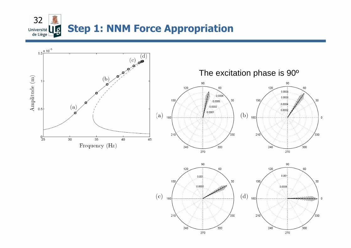
A nonlinear structure vibrates according to one of its NNMs if the degrees of freedom have a phase lag of 90º with respect to the excitation.

Phase lag quadrature criterion:

A linear structure vibrates according to one of its LNMs if the degrees of freedom have a phase lag of 90º with respect to the excitation.


NNM Indicator

32

The excitation phase is 90º


33

Turn off the excitation and track the NNM according to the invariance principle:

« If the motion is initiated on one specific NNM, the remaining NNMs remain quiescent for all time. »

Step 2: NNM Free Decay Identification

34

Numerical experiments of a nonlinear beam (defined as benchmark in the framework of the European COST Action F3 « Structural Dynamics » [8]).

Geometry

Nonlinear EMA (Illustrative Example)

cubic stiffness is realised by means of a very thin beam

For weak excitation, the system behaviour may be considered as linear. When the excitation level increases, the thin beam exhibits large displacements and a nonlinear geometric effect is activated resulting in a stiffening effect at the end of the main beam.

35

Finite Element model

The thin beam is represented by two equivalent grounded

springs: one in translation ( ) and one in rotation ( ).


8 10978002.05 1011

Nonlinear parameter knl(N/m3)

Density(kg/m3)

Young’s modulus(N/m2)

8 10978002.05 1011

Nonlinear parameter knl(N/m3)

Density(kg/m3)

Young’s modulus(N/m2)

36

Theoretical frequency-energy plots

First NNM

NNM shapes

Second NNM

Backbone curve Backbone

curve

NNM shapes


Energy Energy

Freq

uenc

y (H

z)

Freq

uenc

y (H

z)

37

Simulated experiments

Linear proportional damping is considered.

Imperfect force appropriation

From a practical viewpoint, it is useful to study the quality of imperfect force appropriation consisting of a single-point mono-harmonic excitation, i.e., using a single shaker with no harmonics of the fundamental frequency.

The harmonic force p(t) = F sin(ω t) is applied to node 4 of the main beam.

It corresponds to moderate damping; for instance, the modal damping ratio is equal to 1.28% for the first linear normal mode.

MKC 5103 7 += −


38

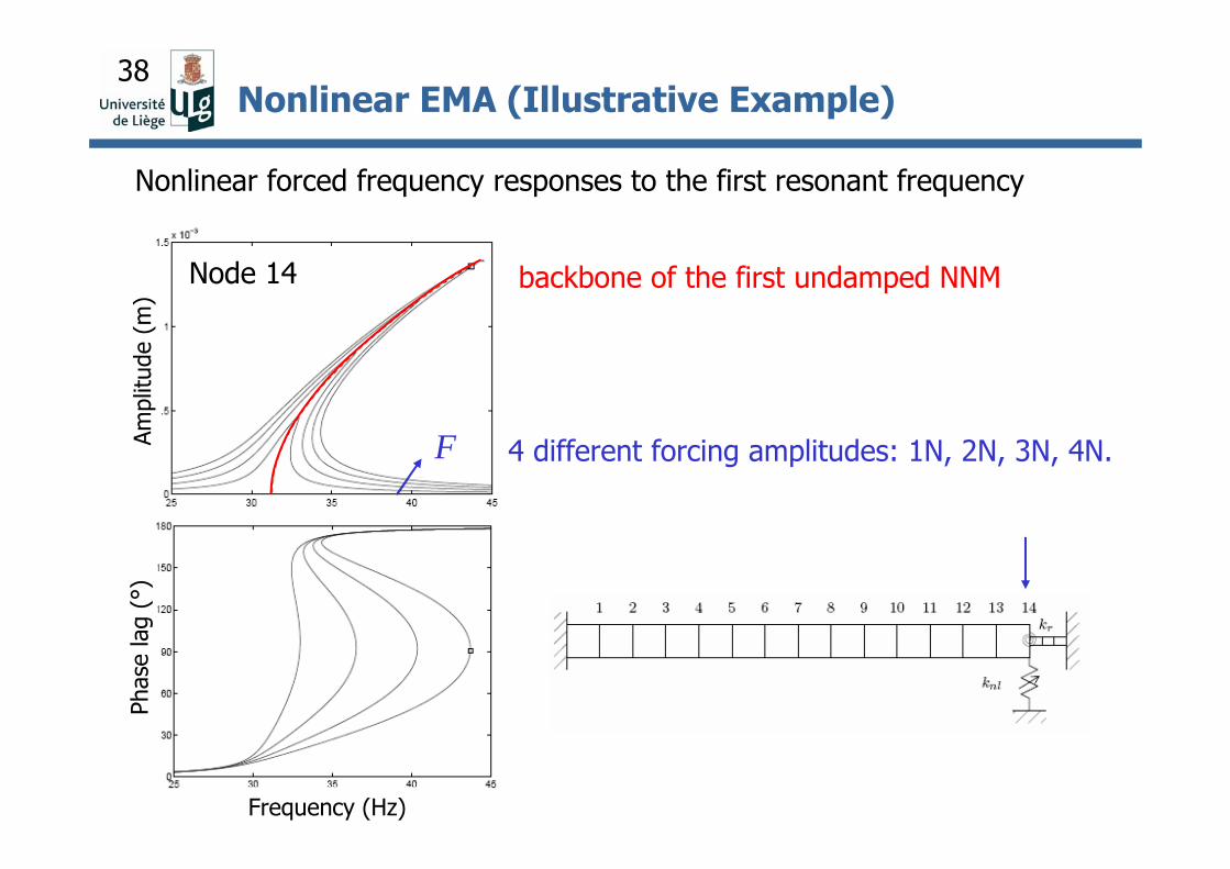
Nonlinear forced frequency responses to the first resonant frequency

backbone of the first undamped NNM

4 different forcing amplitudes: 1N, 2N, 3N, 4N.

Node 14


FAmpl

itude

(m

)Ph

ase

lag

(°)

Frequency (Hz)

39

Observations

• The phase lag quadrature criterion is fulfilled close to resonant frequencies.

• Forced responses at resonance occur in the neighbourhood of NNMs.

• Imperfect appropriation can isolate the NNM of interest (the beam has well-separated modes).

These findings also hold for the second beam NNM.

Time seriesF = 4N

Configuration space


Time (s) Displ. at node 10 (m)

Dis

plac

emen

t (m

)

Dis

pl. a

t no

de 1

4 (m

)

40

Responses along the branch close to the first resonance

Stepped sine excitation procedure for carrying out the NNM forceappropriation (F = 4N) of the damped nonlinear beam.

Phase scatter diagrams of the complex Fourier coefficients of the displacements corresponding to the fundamental frequency for the responses (a), (b), (c) and (d).

Nonlinear EMA (Illustrative Example)Am

plitu

de (

m)

Frequency (Hz)

41

NNM free decay identification

Time series of the displacement at the tip of the main beam (node 14).

Free response of the damped nonlinear beam initiated from the imperfect appropriated forced response

Motion in the configuration space composed of the displacements at nodes 10 and 14.


Time (s) Displacement at node 10 (m)D

ispl

. at

node

14

(m)

Dis

plac

emen

t (m

)

42

Frequency-energy plot of the first NNM of the nonlinear beam.

Theoretical FEP

This FEP was calculated from the time series of the free damped response using the CWT. The solid line is the ridge of the transform.


Experimental FEP

43

Experimental FEP

Backbone

Modal curves Modal shapes


44

Experimental set-up

Benchmark of the European COST Action F3 « Structural Dynamics ».

Experimental Demonstration

Test conditions

• Harmonic excitation of the nonlinear beam.

• Response measured using seven accelerometers.

• Very preliminary results.

45

Total energy (Log scale)

Freq

uenc

y (H

z)

-5 -4.5 -4 -3.5 -3 -2.523

24

25

26

27

28

29

30

Initiate the motion here

Excitation of the 1st NNM of the beam


46

0 0.05 0.1 0.15 0.2 0.25-0.8

-0.6

-0.4

-0.2

0

0.2

0.4

0.6

0.8

Time (s)

Cha

nnel

2 (g

)

0 0.05 0.1 0.15 0.2 0.25-5

-4

-3

-2

-1

0

1

2

3

4

5

Time (s)

Cha

nnel

5 (g

)

0 0.05 0.1 0.15 0.2 0.25-5

-4

-3

-2

-1

0

1

2

3

4

5

Time (s)

Cha

nnel

8 (g

)

-5 -4 -3 -2 -1 0 1 2 3 4 5-5

-4

-3

-2

-1

0

1

2

3

4

5

Channel 5 (g)

Cha

nnel

8 (g

)

Sustained harmonic excitation


47

Burst sine

1.1 1.15 1.2 1.25 1.3 1.35 1.4 1.45 1.5-0.8

-0.6

-0.4

-0.2

0

0.2

0.4

0.6

Time (s)

Cha

nnel

2 (g

)

1.1 1.15 1.2 1.25 1.3 1.35 1.4 1.45 1.5-4

-3

-2

-1

0

1

2

3

4

Time (s)

Cha

nnel

5 (g

)

1.1 1.15 1.2 1.25 1.3 1.35 1.4 1.45 1.5-5

-4

-3

-2

-1

0

1

2

3

4

5

Time (s)

Cha

nnel

8 (g

)

Turn Off the Shaker


48

Total energy (Log scale)

Freq

uenc

y (H

z)

-5 -4.5 -4 -3.5 -3 -2.523

24

25

26

27

28

29

30

Decay along the 1st NNM


49

1.1 1.15 1.2 1.25 1.3 1.35 1.4 1.45 1.5-0.8

-0.6

-0.4

-0.2

0

0.2

0.4

0.6

Time (s)

Cha

nnel

2 (g

)

1.1 1.15 1.2 1.25 1.3 1.35 1.4 1.45 1.5-4

-3

-2

-1

0

1

2

3

4

Time (s)

Cha

nnel

5 (g

)

1.1 1.15 1.2 1.25 1.3 1.35 1.4 1.45 1.5-5

-4

-3

-2

-1

0

1

2

3

4

5

Time (s)

Cha

nnel

8 (g

)

1st NNM of the beam at different energy levels

-5 -4 -3 -2 -1 0 1 2 3 4 5-5

-4

-3

-2

-1

0

1

2

3

4

5

Channel 5

Cha

nnel

8

NNM Extraction


50Outline

1. Introduction




• Parameter Estimation Using POD

• Parameter Estimation Using Nonlinear EMA


51

Description of the structure in terms of its mass, stiffness and

damping properties

Theoretical Approach – Direct Problem

Experimental Approach – Inverse Problem

Structural Model Modal Model Response Model

Response Measurements

Modal Model (Identification) Structural Model

Natural frequencies, Modal damping factors,

Mode shapes

Frequency Response Functions, Impulse Response Functions

Model Updating

Model Updating

52

Parameters for Model Updating (Crucial step!)

The number of parameters :

• should be kept small to avoid problems of ill-conditioning,

• should be chosen with the aim of correcting recognised features in the model.

requires physical insight leads to knowledge-based models.

Methodology

• Estimation of nonlinear parameters only (which will be based on FE updating techniques).

Assumption

• The linear counterpart of the structure is known (updated).

Model Updating

53

Consider the general equation governing the dynamics of a structure

Step 1: definition of a penalty function involving modal features of the system (residual between analytical and measured dynamic behaviour)

Mathematical Background

The measured quantities may be assembled into a measurement vector z.

)(tNL g)x(x,fxKxCxM =+++ &&&&


Model Parameter Estimation Techniques

54

Penalty function methods are based on the Taylor series expansion of the modal data in terms of the unknown parameters

( ) ( ) ( )200

0

ppppzzz

ppOp +−⎥

⎦

⎤⎢⎣

⎡∂∂+=

=

The vector of modal features z depends on parameters p

( )pzz =The choice of parameters is a crucial step in model updating. For nonlinear identification purposes, we will assume that a knowledge-basedmodel exists (the physically meaningful model and the associatedparameters are supposed to be known).

Sensitivity matrix

Initial estimation of the parameters

This expansion is often limited to the first two terms.


55

Define the weighted penalty function

εWεT=JPositive definite weighting matrix

where pSzε Δ−Δ= is the error in the predicted measurements.


⎥⎦

⎤⎢⎣

⎡∂∂=pzS is the sensitivity matrix.

Minimising J with respect to Δp leads to

( ) zWSSWSp Δ=Δ− TT 1

With the assumption that the number of measurements is larger than the number of parameters, the matrix is square and hopefully full rank.

SWST

56

Definition of the measurement vector z containing the modal features.

• In the case of linear systems

• In the case of nonlinear systems

Proper Orthogonal Decomposition

Nonlinear Modal Analysis


( )TTrr

Tii

TT ΦΦΦz ,,,,,,, 11 ωωω KK=

i th eigenvalue

i th mode shape vector

57

Nonlinear Systems

Statistical approach

Proper Orthogonal Decomposition:

Response:

Linear Systems

Deterministic approach

Eigenvalue problem:

Response:

)(tNL p)x(x,fxKxCxM =+++ &&&&)(tpxKxCxM =++ &&&

0ΦMK =− )( 2ω

∑=

=n

iii tt

1)()()( Φx η

TVUX Σ=

∑=

=n

jjj tat

1)()()( ux

Spatial information

Natural frequencies

)sin()cos( tBtA iiiii ωωη +=

Time information

Instantaneous frequencies

Spatial information

Parameter Estimation Using POD

58

Wavelet Transform Instantaneous frequencies

Principle of the method :Minimise the residuals between the bi-orthogonaldecompositions of the measured and simulated data.

Penalty function :

222 )()()( jkj kj

jjiji j

VUJ ∑∑∑∑∑ Δ+ΔΣ+Δ=

Selection of the POMs with the highest POV

X = U Σ VT

POM (Spatial information)

Associated energy

(Mode participation)

Time information


59

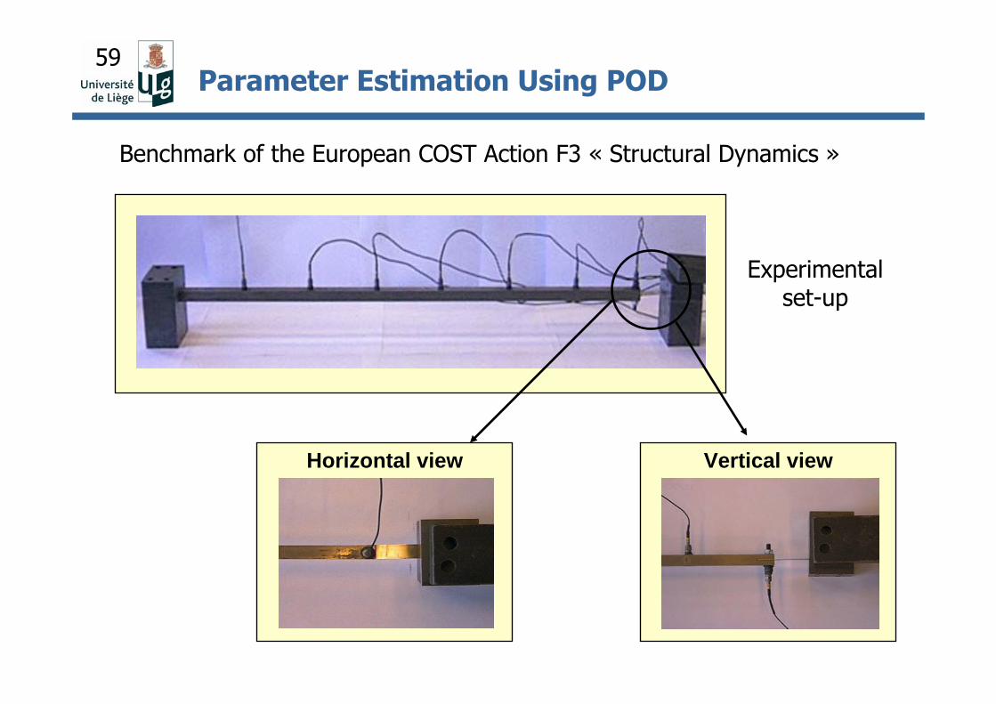
Vertical viewHorizontal view

Experimental set-up

Benchmark of the European COST Action F3 « Structural Dynamics »


60

Finite Element model

The nonlinear stiffening effect of the thin beam is modelled by a nonlinear function in displacement of the form:

where A and α are nonlinear parameters to be identified.

( )xsignxAfnlα=


61

Identification of linear and nonlinear parameters

• 2 parameters : nonlinear stiffness + Young’s modulus

• Penalty function in terms of the first POM

• Simulation time = 0.4 sec

• Gaussian white noise of 1 %

• Nonlinear parameter correction < 10 %

• Linear parameter correction < 50 %

Simulated results


62

Simulated results

Beforeupdating

Afterupdating

Comparison between the original (−) and the reconstructed (--) signals


63

Well-conditioning Ill-conditioning

Non

linea

r pa

ram

eter

Contour Plot

Penalty Function (no WT)Penalty Function (use of WT)

Non

linea

r pa

ram

eter

Linear parameter Linear parameter

Simulated results


64

PSD of the time evolution of the 1st POM

Frequency (Hz)

)()( xsignxAxfnlα=

Experimental results (Vertical set-up)

Model of the nonlinear stiffness

Results of the identification of the nonlinear parameters based on the model updating method:

α = 2.8

A = 1.65 109 N/m2.8Updated

Measured


65

Comparison of the POM

1st POM 2nd POM

3rd POM 4th POM

Experimental results (Vertical set-up)

□ experimental

* nonlinear model(after updating)

o linear model(before updating)


66

Nonlinear MDOF systems

( ) 0=++ xx,fxKxM &&& NL

The concept of Nonlinear Normal Modes (NNMs) is a rigorous extension of the concept of eigenmodes to nonlinear systems.

Caution: the solution is energy-dependent !

Parameter Estimation Using Nonlinear EMA

67

modal shape

Vector of modal features:

i th backbone

( )Tr

Ti

TT zzzz ,,,,1 KK=

( ) ( ) ( ) ( ) ( ) ( ) ( ) ( )( )TTii

Tii

Tii

Tii

Ti K,,,,,,,, 44332211 ΦΦΦΦz ωωωω=

frequency

energy level

Experimental FEP

Backbone

Parameter Estimation Using Nonlinear EMA

68

The Structural Dynamicist’s Toolkit

Theoretical Modelling

VALI

DATI

ONSIM

ULATION

Nonlinear

Systems

UPDATING

ExperimentalMeasurements

Numerical Analysis

Conclusion

69


Theory of Nonlinear

Normal Modes

VALI

DATI

ONSIM

ULATION

Nonlinear

Systems

UPDATING


Numerical Analysis

Conclusion

70


VALI

DATI

ONSIM

ULATION

Nonlinear

Systems

UPDATING


Shooting method+

Continuation algorithms

Conclusion

Theory of Nonlinear

Normal Modes

71


VALI

DATI

ONSIM

ULATION

Nonlinear

Systems

UPDATING

Nonlinear EMA+

Wavelet Transform

Shooting method+

Continuation algorithms

Conclusion

Theory of Nonlinear

Normal Modes

72

1. D. J. Ewins, Modal Testing : theory, practice and application, Second Edition, Research Studies Press LTD, 2000.

2. N. Maia, J. Silva, Theoretical and Experimental Modal Analysis, Research Studies Press LTD, 1997.

3. A.F. Vakakis, L.I. Manevitch, Y.V. Mikhlin, V.N. Pilipchuk, and A.A. Zevin. Normal Modes and Localization in Nonlinear Systems. Wiley series in nonlinear science. John Wiley & Sons, New York, 1996.

4. S.W. Shaw and C. Pierre. Normal modes for nonlinear vibratory systems. Journal of Sound and Vibration, 164(1):85–124, 1993.

5. G. Kerschen, M. Peeters, J.C. Golinval, and A.F. Vakakis. Nonlinear normal modes, part I: A useful framework for the structural dynamicist. Mechanical Systems and Signal Processing, 23(1):170–194, 2009.

6. A.F. Vakakis, O.V. Gendelman, L.A. Bergman, D.M. McFarland, G. Kerschen, and Y.S. Lee. Nonlinear Targeted Energy Transfer in Mechanical and Structural Systems. 2009.

7. P. Panagopoulos, F. Georgiades, S. Tsakirtzis, A.F. Vakakis, and L.A. Bergman. Multi-scaled analysis of the damped dynamics of an elastic rod with an essentially nonlinear end attachment. International Journal of Solids and Structures, 44:6256–6278, 2007.

8. F. Thouverez. Presentation of the ECL benchmark. Mechanical Systems and Signal Processing, 17(1):195–202, 2003.

9. V. Lenaerts, G. Kerschen, J.C. Golinval, Proper Orthogonal Decomposition for Model Updating of Non-linear Mechanical Systems, Journal of Mechanical Systems and Signal Processing, 15(1), pp.31-43, 2001

10. M. Peeters, G. Kerschen, J.C. Golinval, Modal Testing of Nonlinear Vibrating Structures Based on a Nonlinear Extension of Force Appropriation, Proc. of the ASME IDETC/CIE 2009, Aug. 30-Sept. 2, 2009, San Diego, USA.

11. M. Peeters, R. Viguié, G. Sérandour, G. Kerschen, and J.C. Golinval. Nonlinear normal modes, part II: Toward a practical computation using numerical continuation techniques. Mechanical Systems and Signal Processing, 23(1):195–216, 2009.

12. T.P. Le and P. Argoul. Continuous wavelet transform for modal identification using free decay response. Journal of Sound and Vibration, 277(1-2):73–100, 2004.

References / Further Readings

73

Thank you for your attention.

parameter estimation and structural model updating using ... · 2 outline 1. introduction 2....

Documents