part 15: basics of physical db design

15. Basics of Physical Database Design 15-1

Part 15: Basics ofPhysical DB Design

References:• Elmasri/Navathe:Fundamentals of Database Systems, 3rd Edition, 1999.

Chapter 6, “Index Structures for Files”Section 16.3, “Physical Database Design in Relational Databases”

• Silberschatz/Korth/Sudarshan: Database System Concepts, 3rd Edition.Chap. 11: “Indexing and Hashing” (only parts of Sections 11.1–3, 11.8)

• Kemper/Eickler: Datenbanksysteme (in German), 4th Ed., Ch. 7, Oldenbourg, 2001.

• Ramakrishnan: Database Management Systems, Mc-Graw Hill, 1998, Chap. 4: “FileOrganizations and Indexes”, Chap. 5: “Tree-Structured Indexing”, Chap. 16: “PhysicalDatabase Design and Tuning”.

• Corey/Abbey/Dechichio/Abramson: Oracle8 Tuning. ORACLE Press, 1998.

• Oracle 8i Concepts, Release 2 (8.1.6), Oracle Corporation, 1999, Part No. A76965-01.0-23 ff: “Indexes”

• Oracle 8i Administrator’s Guide, Release 2 (8.1.6), Oracle Corporation, 1999, PartNo. A76956-01. Chapter 14: “Managing Indexes”.

• Oracle 8i Designing and Tuning for Performance, Release 2 (8.1.6), Oracle Corporation,1999, Part No. A76992-01. Chapter 12: “Data Access Methods”.

• Oracle 8i SQL Reference, Release 2 (8.1.6), Oracle Corp., 1999, Part No. A76989-01.CREATE INDEX, page 7-291 ff.

• Gray/Reuter: Transaction Processing, Morgan Kaufmann, 1993, Chapter 15.

• Lipeck: Skript zur Vorlesung Datenbanksysteme (in German), Univ. Hannover, 1996.

Stefan Brass: Datenbanken I Universitat Halle, 2011


Objectives

After completing this chapter, you should be able to:

• enumerate necessary input data for physical design.

• explain the effects of buffering disk blocks in main

memory.

• explain the basic structure of a B+-tree.

• explain which queries can be evaluated faster using

an index.

• explain why indexes have not only advantages.

• formulate the basic CREATE INDEX command in SQL.



Overview

1. General Remarks

2. B+-Tree Indexes

3. Advantages and Disadvantages of Indexes

4. Other Physical Design Issues



Motivation (1)

• Consider a table with information about customers:

CUSTOMERS

CUSTNO FIRST_NAME LAST_NAME · · ·1000001 John Smith · · ·1000002 Ann Miller · · ·1000003 David Meyer · · ·

... ... ... ...

• Assume further that this table is relatively big.E.g. there are 2 Million customers (rows). If the table has columnsFIRST_NAME, LAST_NAME, STREET, CITY, STATE, ZIP, PHONE, EMAIL, the ave-rage disk space per row might be about 100 byte, and (includingcertain overheads), the table will be about 230 MB large.



Motivation (2)

• Suppose that a specific customer record is queried:

SELECT *

FROM CUSTOMERS

WHERE CUSTNO = 1000002

• Without special data structures, the DBMS simply

checks CUSTNO = 1000002 for each row of the table.This is called a “Full Table Scan”. All rows are read from the disk.

• The query will run about 12 seconds.Currently (2001), 20 MB/s in a sequential scan are quite typical.12 seconds are significantly too long for interactive work. If 100 clerksuse the DB, each can pose a query only every 20 minutes.



Physical Database Design (1)

• The purpose of physical DB design is to ensure that

the DBS meets the performance requirements.

• Requires knowledge of / estimates for:

� Size of the tables, distribution of data.

� How often each application program is executed.

� Which queries and updates are contained in each

application program.

� Performance requirements.Interactive programs usually need fast answers (below 1–2 se-conds), some seldomly executed programs could run a little lon-ger, and reports may be generated over night.



Physical Database Design (2)

• Since these parameters are difficult to estimate and

change over time, be prepared to repeat the physi-

cal design step from time to time.

Creating a new index is simple in relational systems. However, havingto buy entirely new hardware because performance criteria are notmet, is a problem. It is necessary to think about realistic system loadsduring the design. There are tools for simulating given loads. Don’tstart using the system before ascertaining that it will work.

• Physical design depends on the chosen DBMS.

The DBMS, how it works, and its performance tuning parametersmust be understood very well.



Disks

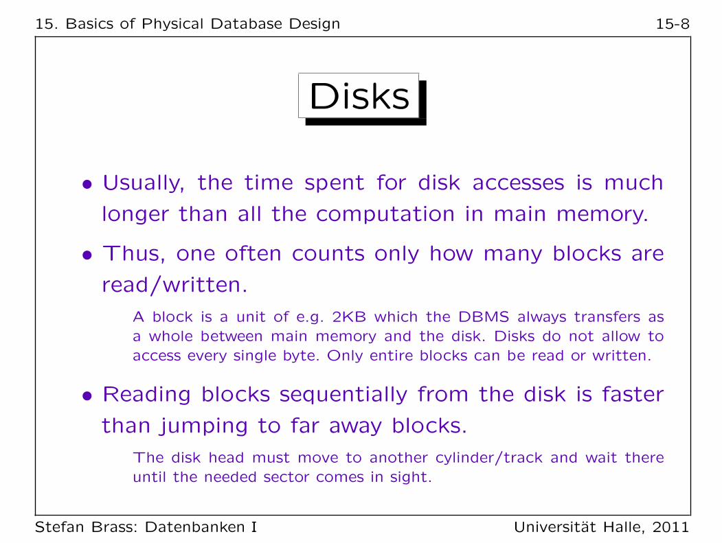
• Usually, the time spent for disk accesses is much

longer than all the computation in main memory.

• Thus, one often counts only how many blocks are

read/written.

A block is a unit of e.g. 2KB which the DBMS always transfers asa whole between main memory and the disk. Disks do not allow toaccess every single byte. Only entire blocks can be read or written.

• Reading blocks sequentially from the disk is faster

than jumping to far away blocks.

The disk head must move to another cylinder/track and wait thereuntil the needed sector comes in sight.



Buffering

• A copy of the most recently read blocks is kept in

main memory (buffer, cache).Reading blocks from the disk is much slower than memory accesses.Goal: Many block requests (90%) can be answered from the cache.

• Not all blocks can be kept in memory, since the DB

is normally much bigger than the main memory.E.g. the DB is several GB, the main memory 256MB.

• The first execution of a query takes much longer

than executing the same query a second time.For small DBs, soon the entire DB will be in main memory, and diskaccesses are only needed to make updates durable (not for queries).



Overview

1. General Remarks

2. B+-Tree Indexes





B+-Trees (1)

• DBMS offer a variety of special access structures

to find the requested record without reading the

entire file. The most common one is the B+-tree.

Every modern DBMS contains some variant of B-trees. In addition itmay support other specialized index structures.

• B-trees are named after Rudolf Bayer.

Bayer/McCreight: Organization and Maintenance of Large OrderedIndices. Acta Informatica 1(3), 173–189, 1972.

• B∗-trees and B+-trees are (normally) synonyms.



B+-Trees (2)

• In general, B-trees work like standard binary search

trees:

7 root

4

2

leaf

5

leaf

9

8

leaf

height 3

The search starts in the root node. If the searched value is less thanthe value in the root node, the search continues in the left subtree,if it is larger, the search continues in the right subtree.



B+-Trees (3)

• In a B-tree, the branching factor (fan out) is much

higher than 2.Anyway a whole block must be read from the disk.

• Normal binary trees can degenerate to a linear list.

B-trees are balanced, so this cannot happen.E.g. if values are inserted in ordered sequence, they are always insertedto the right in a normal binary tree.

• In a B+-tree (not in a B-tree) the values in inner

nodes (non-leaves) are repeated in the leaf nodes.The tree height might decrease, since the pointer to the row is neededonly in the leaf nodes. Also one can easily get a sorted sequence.



B+-Trees (4)

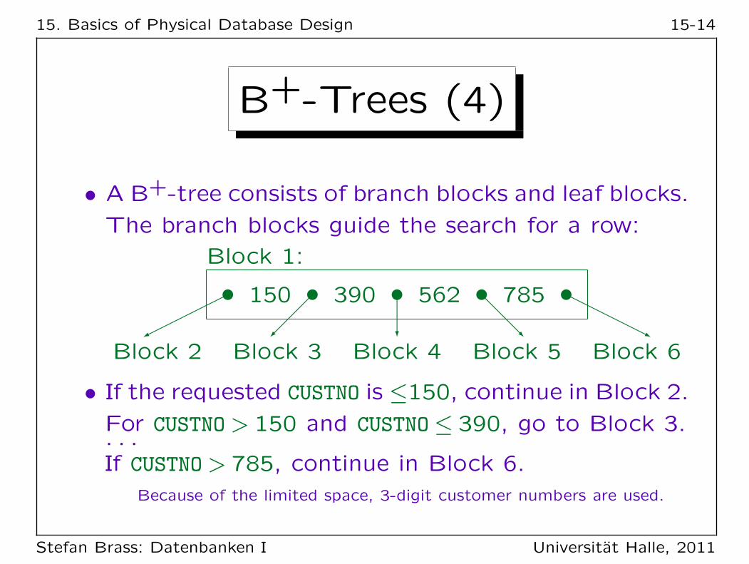
• A B+-tree consists of branch blocks and leaf blocks.

The branch blocks guide the search for a row:

Block 1:

Block 2

150

Block 3

390

Block 4

562

Block 5

785

Block 6

• If the requested CUSTNO is ≤150, continue in Block 2.

For CUSTNO> 150 and CUSTNO≤ 390, go to Block 3.. . .If CUSTNO> 785, continue in Block 6.

Because of the limited space, 3-digit customer numbers are used.



B+-Trees (5)

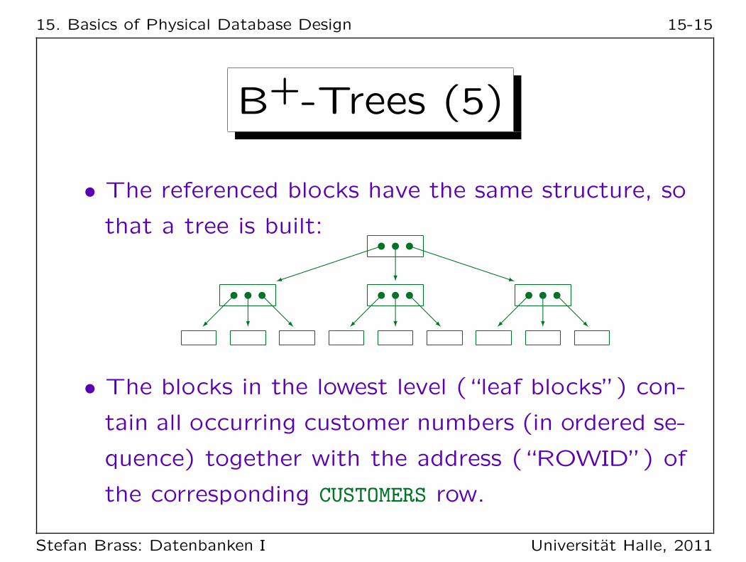
• The referenced blocks have the same structure, so

that a tree is built:

• The blocks in the lowest level (“leaf blocks”) con-

tain all occurring customer numbers (in ordered se-

quence) together with the address (“ROWID”) of

the corresponding CUSTOMERS row.



B+-Trees (6)

390 540}

Branch Block

230 390 410 540 670 780}

Leaf Blocks

CUSTOMERS

CUSTNO · · ·

410 · · ·230 · · ·670 · · ·540 · · ·780 · · ·390 · · ·



B+-Trees (7)

• In a B-tree, all leaf blocks must have the same

distance (number of edges) from the root. Thus

B-trees are balanced.

This ensures that the chain of links which must be followed in orderto access a leaf node is never long. For B-trees, the complexity ofsearching (tree height) is O(log(n)), where n is the number of entries.

• Nodes in the same tree can contain differently many

values, but each node must be at least half full.

(Except the root, which might contain only a single customer num-ber.) If the blocks had to be completely full, an insertion of one tuplecould require a change of every block in the tree. With the relaxedrequirement, insertion/deletion are possible in O(log(n)).



B+-Trees (8)

• Insertion Algorithm:

� Search the leaf node into which the new value

must be inserted.

� If that node has still empty space: insert. Done.

� Otherwise, split the leaf node in the middle (one

full node → two half full ones), do the insertion.

� Now the branch block above must contain one

additional value (middle value in splitted node).

� If there is still space, ok. Otherwise split the

branch block. And so on up to the root.



B+-Trees (9)

Exercise:

• Consider again the B+-tree from Slide 15-16:

390 540

230 390 410 540 670 780

• Assume that each node can contain at most two

values (and must contain at least one value).

• Insert the value 123.

• Give an example for a value that can now be inser-

ted without splitting any further nodes.



B+-Trees (10)

• Real branching factors are much higher than shown

above.

• A block of 2KB can probably contain about 100

customer numbers and the corresponding ROWIDs.

Height Min. Num. Rows Max. Num. Rows

1 1 1002 2 ∗ 50 =100 1002 = 100003 2 ∗ 502 = 5000 1003 = 10000004 2 ∗ 503 = 250000 1004 = 100000000

Height 1: Only root, which is at the same time leaf.Height 2: Root as branch node, plus leaf blocks, as on Slide 15-16.



B+-Trees (11)

• For the CUSTOMERS table with 2000000 entries, the

B-tree will have height 4.

Height 5 would require at least 2 ∗ 504 = 12.5 mio rows.

• A tree of height 4 requires 5 block accesses to get

the row for a given customer number.

Four for the index and one for fetching the row from the table with theROWID obtained from the index. In rare circumstances (“migratedrow”), 6 block accesses would be required in total.

• The query can be executed in 50ms.

Fast modern disks need about 10ms per random block access.One disk can support about 14 such queries per second (70% load).



B+-Trees (12)

• Table accesses via an index profit from caching of

disk blocks:

E.g. it is very likely that the root node of the index

and some part of the next level will be in the buffer.

• Since the height of the B-tree grows only loga-

rithmically in the number of rows, B-trees never

become very high.

Heights greater than 4 or 5 are rare in practice.



B+-Trees (13)

• The index on CUSTNO was a unique index — there

is only one row for every value (CUSTNO is a key).

• B-trees also support non-unique indexes, e.g. on

LAST_NAME. Then the leaf blocks can contain more

than one row address for the same column value.Although LAST_NAME is not a key of the table, it is sometimes calledthe “search key” of the B-tree.

• It is also possible to create B-trees over the com-

bination of two or more columns.Then the indexed values are basically the concatenation of columnvalues (with e.g. a separator character).



B+-Trees (14)

Brown}

Branch Block

Brass Brown Meyer Smith}

Leaf Blocks

CUSTOMERS

LAST_NAME · · ·

Brass · · ·Brown · · ·Smith · · ·Meyer · · ·Brass · · ·Smith · · ·



B+-Trees (15)

• A high branching factor (and thus a small tree

height) is possible only if the data in the indexed

column is not too long.

E.g. an index over a column that contains strings of length 500 willneed a higher tree (which still grows logarithmically). In Oracle, theindexed values may not be larger than about half of the block size.

• It suffices to store a prefix of the actual data in the

branch blocks if this prefix already allows discrimi-

nation between the blocks on the next level.

The full version of column data is anyway stored in the leaf blocks.In the above example, it suffices to store ’B’ in the root node.



Overview

1. General Remarks

2. B+-Tree Indexes





Applications of Indexes (1)

• An index on the column A of the relation R is espe-

cially useful for equality conditions A = c on tuple

variables over the relation R.In relational algebra, this corresponds to the selection σA=c(R).

• A B+-tree index can also be used for <, <=, >, >=

conditions (range queries, LIKE with known prefix).

• However, indexes are only useful when only a small

percentage of the rows are retrieved via the index.If many rows satisfy the condition, a full table scan is faster: Sequentialreading of blocks is faster than random accesses, and all rows in ablock are together processed (in an index lookup only single rows).




• An index can be used even if there are other con-

ditions besides the one supported by the index:

SELECT *

FROM CUSTOMERS

WHERE LAST_NAME = ’Smith’

AND CITY = ’Pittsburgh’

• If there is an index on the attribute LAST_NAME, the

DBMS can use it to retrieve all rows that satisfy the

first condition, and then simply check the second

condition for each such row.




• A join can be evaluated using an index on one of

the joined columns, e.g.:

SELECT C.LAST_NAME

FROM INVOICES I, CUSTOMERS C

WHERE I.AMOUNT > 20000

AND C.CUSTNO = I.CUSTNO

• E.g. the DBMS can first find large invoices I and

then use an index on CUSTOMERS(CUSTNO) to retrieve

the customer data for each such invoice.

Each single row I contains a specific customer number, for which onecan use the index to find the matching row C.




• Some queries can even be answered entirely out of

the index, without accessing the table itself: E.g. is

there a customer with a given number?

This is important for enforcing key/foreign key constraints.

• Sorting might sometimes profit from an index.

This may speed up ORDER BY, GROUP BY, DISTINCT. The leaves of theB+-tree contain all values in sorted sequence. However, this is reallyeffective only in combination with a range query or if the query can beanswered entirely out of the index. Otherwise accessing all rows of thetable in random order might be slower than using e.g. the Mergesortalgorithm (which does several sequential passes over the data).




• Indexes on combinations of two or more columns of

a table will especially speed up queries that provide

values for all these columns:

SELECT *

FROM CUSTOMERS

WHERE FIRST_NAME=’John’ AND LAST_NAME=’Smith’

• If the index is a B-tree, it can also be used as an

index for the first column (or in general a prefix).The first column of the combination is the main sorting criterion forthe index. Here an index on LAST_NAME, FIRST_NAME would probably bemore useful than the other way round. It could be used also as anindex on LAST_NAME (it is slightly less efficient than a pure index).




Exercise:

• Consider the following query:

SELECT C.FIRST_NAME, C.LAST_NAME, C.PHONE

FROM CUSTOMERS C, ORDERS O, ORDER_DETAILS D

WHERE D.PRODNO = 123

AND C.CITY = ’Pittsburgh’

AND O.ORD_DATE >= ’01-JAN-02’

AND C.CUSTNO = O.CUSTNO AND O.ORDNO = D.ORDNO

• Which indexes could be useful for evaluating the

query? Sketch two different evaluation possibilities.

What information would the DBMS need for deciding which evaluationmethod is better?



Disadvantages of Indexes

• Indexes use disk space.

The example index needs 30-50% of the space of the table.

• Queries become faster, but updates become slower

because the indexes must be updated, too.

• Query optimization becomes slower: More alterna-

tives for evaluating the query must be considered.

But it might be possible to amortize the cost of query optimizationover many executions of the same query.

• A full table scan can be much faster if nearly all

blocks must be accessed anyway.



Hints for Selecting Indexes

• Check whether the query optimizer really uses the

indexes.

DBMS usually offer the possibility to see the result of query optimi-zation (query evaluation plans, internal query programs).

• It makes no sense to declare indexes on small tables.

Except the indexes needed to enforce keys, see below.

• Do not declare too many indexes on tables that are

often updated.

• Normally, an index is useful only if the condition is

satisfied only by a small percentage of the rows.



Indexes in SQL (1)

• SQL command for creating an index (not SQL-92):

CREATE

UNIQUE

INDEX Name

ON Table ( Column )

,

• E.g.: CREATE INDEX CUSTIND1 ON CUSTOMERS(CITY)



Indexes in SQL (2)

• The CREATE INDEX command is not contained in the

SQL standards, but it is supported by most DBMS.The SQL standards do not treat physical storage concepts.

• UNIQUE means that for every value for the index co-

lumn there is only one tuple.I.e. the index column is a key. Older SQL versions had no key decla-rations, so a unique indexes were used.

• Most DBMS automatically create a unique index

for key constraints (PRIMARY KEY and UNIQUE).Thus the keys are enforced as before by means of unique indexes.It would be wrong to explicitly create another index for a key.



Indexes in SQL (3)

• Creating an index on a large table can take quite

some time, need a lot of temporary disk space, and

lock the entire table.

One should not experiment with indexes during the main productionhours. On some systems (e.g. DB2, but not Oracle), it might benecessary to rebind (re-optimize) application programs after relevantindexes were changed.

• Command for deleting indexes:

DROP INDEX Name

• E.g.: DROP INDEX CUSTIND1



Overview

1. General Remarks

2. B+-Tree Indexes





Physical Design Issues (1)

• The index selection, i.e. deciding which indexes to

create, is the classical physical design issue. But

there is much more to do.

• Normally the table itself is stored as a “heap file”

(without any specific order), but even for that there

are various storage parameters.

E.g. how much space in a block should be kept free for updates thatmake a row longer (because of physical pointers from indexes, it isnot good to “migrate” a row to a different block). One should alsoensure that the table is stored sequentially in one chunk of disk space(or only a few big pieces), not scattered over the entire disk (in manysmall pieces). Thus, one must define a storage size.



Physical Design Issues (2)

• Database management systems offer other access

structures besides B-trees, e.g. hash methods.

Oracle allows clustering tables together (good for joins). Instead ofhaving separate indexes and table, it might also be possible to storethe table data directly in the index (index-organized table).

• The distribution of tables etc. among different disks

is also important for performance.

Tables can be split into several parts (horizontal/vertical partitioning).

• In exceptional cases, tables could be denormalized.

One pays for the performance gain with programmer time and lessflexibility for changes.


part 15: basics of physical db design

Documents