Security Level:

HUAWEI TECHNOLOGIES CO., LTD.

www.huawei.com

Slide title :40-47pt

Slide subtitle :26-30pt

Color::white

Corporate Font :

FrutigerNext LT Medium

Font to be used by customers and

partners :

Arial

Mathematical and Algorithmic Sciences Lab

Massive MIMO for Maximum Spectral

Efficiency

Mérouane Debbah

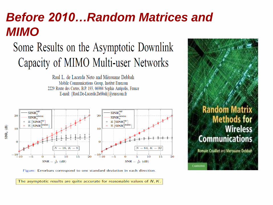
Before 2010…Random Matrices and

MIMO

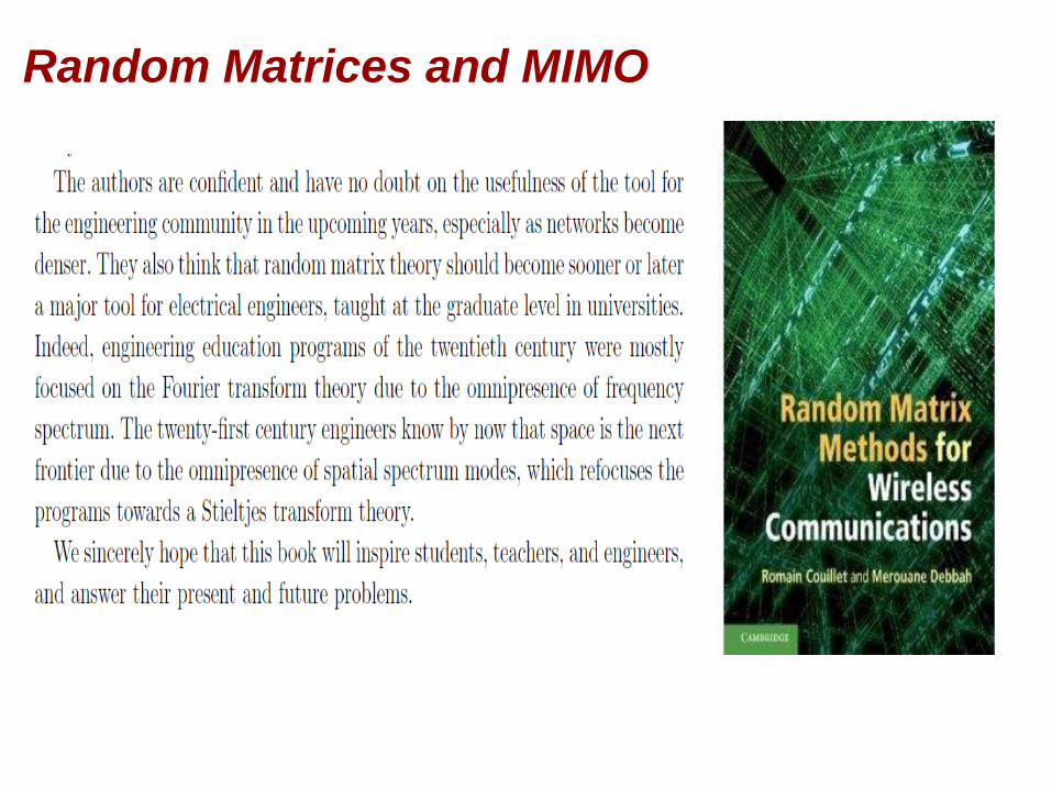
Random Matrices and MIMO

Green Touch Initiative

J. Hoydis, S. ten Brink, M. Debbah, “Massive MIMO in the UL/DL of Cellular

Networks: How Many Antennas Do We Need?,” IEEE Journal on Selected Areas

in Communications, 2013. IEEE Leonard G. Abraham Prize

6

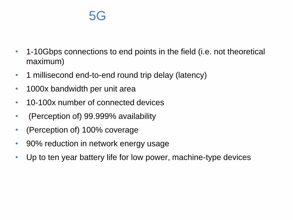
5G

• 1-10Gbps connections to end points in the field (i.e. not theoretical

maximum)

• 1 millisecond end-to-end round trip delay (latency)

• 1000x bandwidth per unit area

• 10-100x number of connected devices

• (Perception of) 99.999% availability

• (Perception of) 100% coverage

• 90% reduction in network energy usage

• Up to ten year battery life for low power, machine-type devices

Massive MIMO as one of the operating of

5G

E. Bjornson, L. Sanguinetti, J. Hoydis and M. Debbah, "Designing Multi-User MIMO for

Energy Efficiency: When is Massive MIMO the Answer? », IEEE Wireless Communications

and Networking Conference (WCNC) 2014, Istanbul, Turkey, BEST PAPER AWARD.

9

The Three Phases of Massive MIMO

Every great scientific truth goes through three phases.

• 1) First, people deny it.

• 2) Second, they say it conflicts with the physics (engineering)

principles

• 3) Third, they say they’ve known it all along.

10

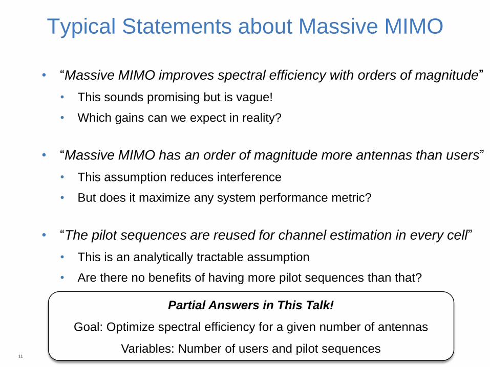
Typical Statements about Massive MIMO

• “Massive MIMO improves spectral efficiency with orders of magnitude”

• This sounds promising but is vague!

• Which gains can we expect in reality?

• “Massive MIMO has an order of magnitude more antennas than users”

• This assumption reduces interference

• But does it maximize any system performance metric?

• “The pilot sequences are reused for channel estimation in every cell”

• This is an analytically tractable assumption

• Are there no benefits of having more pilot sequences than that?

11

Partial Answers in This Talk!

Goal: Optimize spectral efficiency for a given number of antennas

Variables: Number of users and pilot sequences

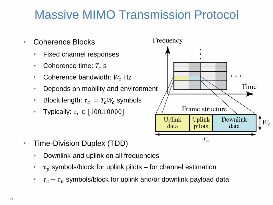
Massive MIMO Transmission Protocol

• Coherence Blocks

• Fixed channel responses

• Coherence time: 𝑇𝑐 s

• Coherence bandwidth: 𝑊𝑐 Hz

• Depends on mobility and environment

• Block length: 𝜏𝑐 = 𝑇𝑐𝑊𝑐 symbols

• Typically: 𝜏𝑐 ∈ [100,10000]

• Time-Division Duplex (TDD)

• Downlink and uplink on all frequencies

• 𝜏𝑝 symbols/block for uplink pilots – for channel estimation

• 𝜏𝑐 − 𝜏𝑝 symbols/block for uplink and/or downlink payload data

12

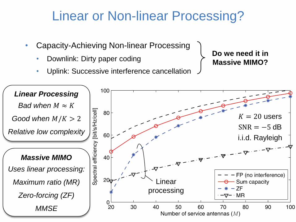
Linear or Non-linear Processing?

• Capacity-Achieving Non-linear Processing

• Downlink: Dirty paper coding

• Uplink: Successive interference cancellation

13

Do we need it in

Massive MIMO?

Linear Processing

Bad when 𝑀 ≈ 𝐾

Good when 𝑀/𝐾 > 2

Relative low complexity

𝐾 = 20 users

SNR = −5 dB

i.i.d. Rayleigh

Massive MIMO

Uses linear processing:

Maximum ratio (MR)

Zero-forcing (ZF)

MMSE

Linear

processing

Channel Acquisition in Massive MIMO

• Limited Number of Pilots: 𝜏𝑝 ≤ 𝜏𝑐

• Must use same pilot sequence in several cells

• Base stations cannot tell some users apart:

Essence of pilot contamination

• Coordinated Pilot Allocation

• Allocate pilots to users to reduce contamination

• Scalability → No signaling between BSs

• Solution: Non-universal pilot reuse

• Pilot reuse factor 𝑓 ≥ 1

• Users per cell: 𝐾 =𝜏𝑝

𝑓

• 𝒫𝑗(𝑓): Cells with same pilots as BS 𝑗

• Higher 𝑓 → Fewer users per cell,

but fewer interferers in 𝒫𝑗 14 Reuse 𝑓 = 4 Reuse 𝑓 = 1 Reuse 𝑓 = 3

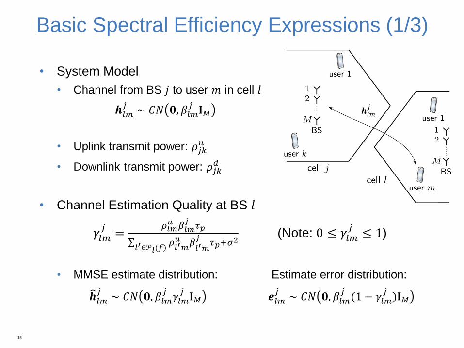
Basic Spectral Efficiency Expressions (1/3)

• System Model

• Channel from BS 𝑗 to user 𝑚 in cell 𝑙

𝒉𝑙𝑚𝑗

∼ 𝐶𝑁 𝟎, 𝛽𝑙𝑚𝑗𝐈𝑀

• Uplink transmit power: 𝜌𝑗𝑘𝑢

• Downlink transmit power: 𝜌𝑗𝑘𝑑

• Channel Estimation Quality at BS 𝑙

𝛾𝑙𝑚𝑗=

𝜌𝑙𝑚𝑢 𝛽𝑙𝑚

𝑗𝜏𝑝

𝜌𝑙′𝑚𝑢

𝑙′∈𝒫𝑙(𝑓)𝛽𝑙′𝑚

𝑗𝜏𝑝+𝜎

2 (Note: 0 ≤ 𝛾𝑙𝑚

𝑗≤ 1)

• MMSE estimate distribution: Estimate error distribution:

𝒉 𝑙𝑚𝑗

∼ 𝐶𝑁 𝟎, 𝛽𝑙𝑚𝑗𝛾𝑙𝑚𝑗𝐈𝑀 𝒆𝑙𝑚

𝑗∼ 𝐶𝑁 𝟎, 𝛽𝑙𝑚

𝑗(1 − 𝛾𝑙𝑚

𝑗)𝐈𝑀

15

𝒉𝑙𝑚𝑗

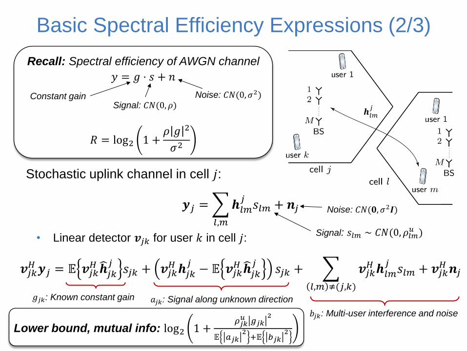
Basic Spectral Efficiency Expressions (2/3)

Stochastic uplink channel in cell 𝑗:

𝒚𝑗 = 𝒉𝑙𝑚𝑗𝑠𝑙𝑚

𝑙,𝑚

+ 𝒏𝑗

• Linear detector 𝒗𝑗𝑘 for user 𝑘 in cell 𝑗:

𝒗𝑗𝑘𝐻 𝒚𝑗 = 𝔼 𝒗𝑗𝑘

𝐻 𝒉 𝑗𝑘𝑗

𝑠𝑗𝑘 + 𝒗𝑗𝑘𝐻 𝒉𝑗𝑘

𝑗− 𝔼 𝒗𝑗𝑘

𝐻 𝒉 𝑗𝑘𝑗

𝑠𝑗𝑘 + 𝒗𝑗𝑘𝐻 𝒉𝑙𝑚

𝑗𝑠𝑙𝑚

𝑙,𝑚 ≠(𝑗,𝑘)

+ 𝒗𝑗𝑘𝐻 𝒏𝑗

16

𝒉𝑙𝑚𝑗

Recall: Spectral efficiency of AWGN channel

𝑦 = 𝑔 ⋅ 𝑠 + 𝑛

𝑅 = log2 1 +𝜌 𝑔 2

𝜎2

Constant gain Noise: 𝐶𝑁(0, 𝜎2) Signal: 𝐶𝑁(0, 𝜌)

Signal: 𝑠𝑙𝑚 ∼ 𝐶𝑁(0, 𝜌𝑙𝑚𝑢 )

Noise: 𝐶𝑁(𝟎, 𝜎2𝑰)

𝑔𝑗𝑘: Known constant gain 𝑎𝑗𝑘: Signal along unknown direction

𝑏𝑗𝑘: Multi-user interference and noise

Lower bound, mutual info: log2 1 +𝜌𝑗𝑘𝑢 𝑔𝑗𝑘

2

𝔼 𝑎𝑗𝑘2+𝔼 𝑏𝑗𝑘

2

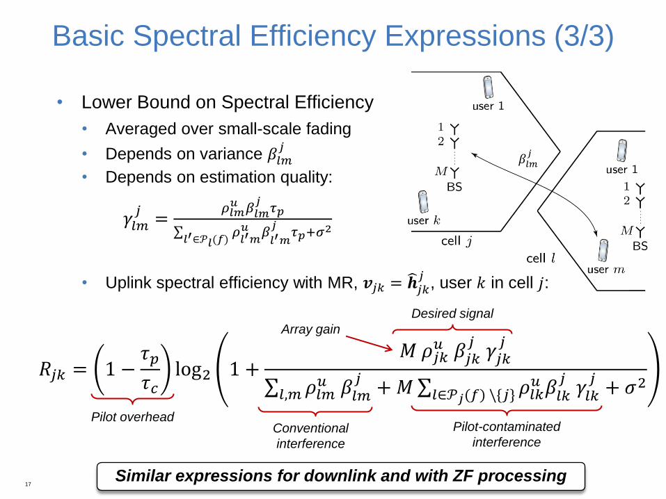
Basic Spectral Efficiency Expressions (3/3)

• Lower Bound on Spectral Efficiency

• Averaged over small-scale fading

• Depends on variance 𝛽𝑙𝑚𝑗

• Depends on estimation quality:

𝛾𝑙𝑚𝑗=

𝜌𝑙𝑚𝑢 𝛽𝑙𝑚

𝑗𝜏𝑝

𝜌𝑙′𝑚𝑢

𝑙′∈𝒫𝑙(𝑓)𝛽𝑙′𝑚

𝑗𝜏𝑝+𝜎

2

• Uplink spectral efficiency with MR, 𝒗𝑗𝑘 = 𝒉 𝑗𝑘𝑗

, user 𝑘 in cell 𝑗:

17

Pilot overhead Conventional

interference

Pilot-contaminated

interference

Desired signal

Similar expressions for downlink and with ZF processing

Array gain

𝛽𝑙𝑚𝑗

𝑅𝑗𝑘 = 1 −𝜏𝑝

𝜏𝑐log2 1 +

𝑀 𝜌𝑗𝑘𝑢 𝛽𝑗𝑘

𝑗 𝛾𝑗𝑘

𝑗

𝜌𝑙𝑚𝑢 𝛽𝑙𝑚

𝑗+𝑀 𝜌𝑙𝑘

𝑢 𝛽𝑙𝑘𝑗

𝑙∈𝒫𝑗(𝑓) \{𝑗} 𝛾𝑙𝑘

𝑗𝑙,𝑚 + 𝜎2

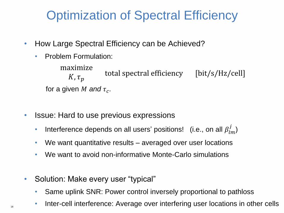
Optimization of Spectral Efficiency

• How Large Spectral Efficiency can be Achieved?

• Problem Formulation:

maximize𝐾, 𝜏𝑝

total spectral efficiency [bit/s/Hz/cell]

for a given 𝑀 and 𝜏𝑐.

• Issue: Hard to use previous expressions

• Interference depends on all users’ positions! (i.e., on all 𝛽𝑙𝑚𝑗

)

• We want quantitative results – averaged over user locations

• We want to avoid non-informative Monte-Carlo simulations

• Solution: Make every user “typical”

• Same uplink SNR: Power control inversely proportional to pathloss

• Inter-cell interference: Average over interfering user locations in other cells 18

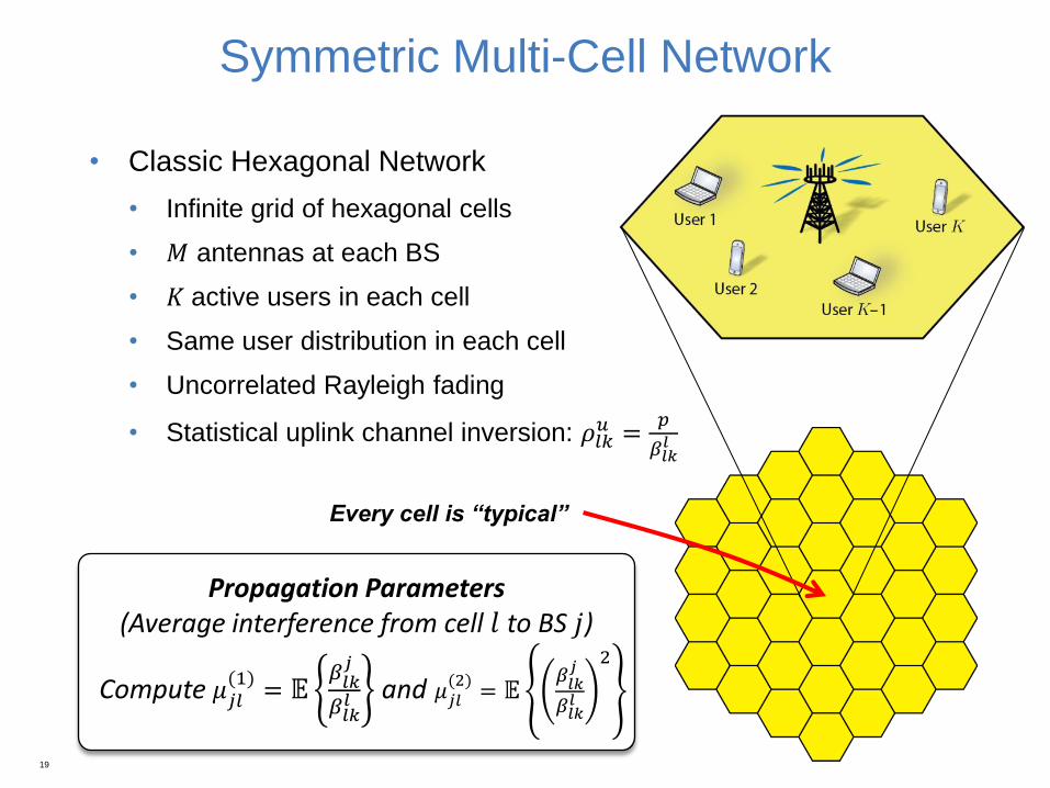
Symmetric Multi-Cell Network

• Classic Hexagonal Network

• Infinite grid of hexagonal cells

• 𝑀 antennas at each BS

• 𝐾 active users in each cell

• Same user distribution in each cell

• Uncorrelated Rayleigh fading

• Statistical uplink channel inversion: 𝜌𝑙𝑘𝑢 =

𝑝

𝛽𝑙𝑘𝑙

19

Every cell is “typical”

Propagation Parameters (Average interference from cell 𝑙 to BS 𝑗)

Compute 𝜇𝑗𝑙(1)

= 𝔼𝛽𝑙𝑘𝑗

𝛽𝑙𝑘𝑙 and 𝜇𝑗𝑙

(2)= 𝔼

𝛽𝑙𝑘𝑗

𝛽𝑙𝑘𝑙

2

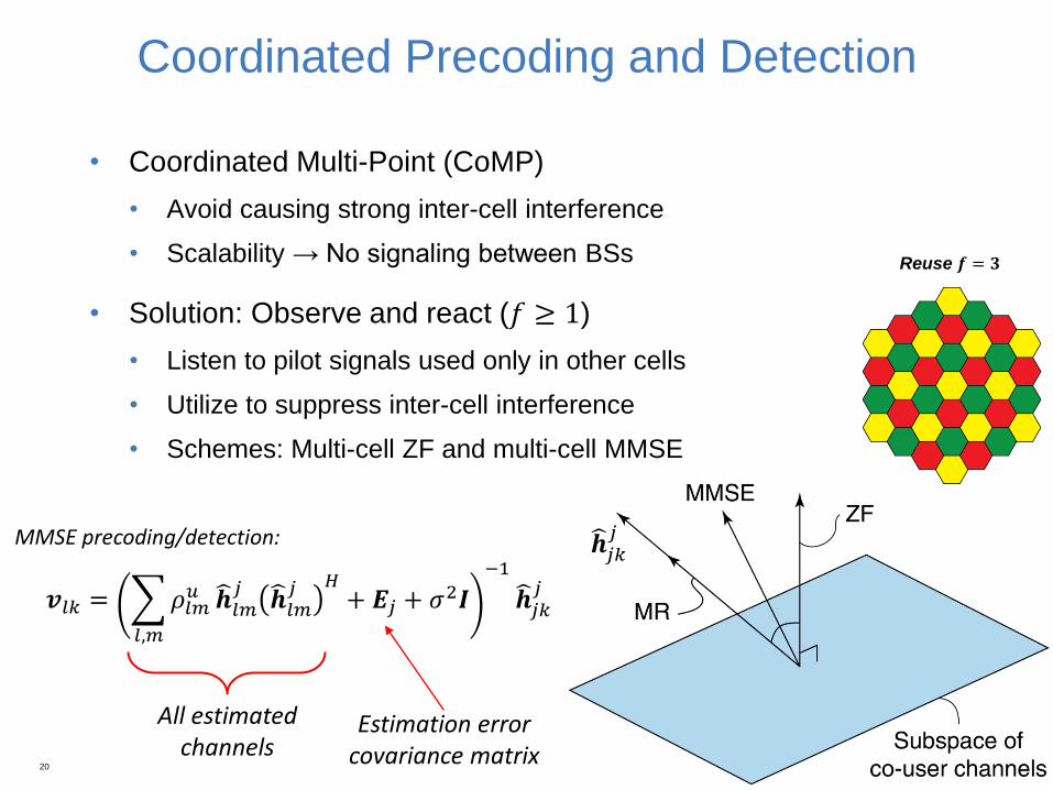
Coordinated Precoding and Detection

• Coordinated Multi-Point (CoMP)

• Avoid causing strong inter-cell interference

• Scalability → No signaling between BSs

• Solution: Observe and react (𝑓 ≥ 1)

• Listen to pilot signals used only in other cells

• Utilize to suppress inter-cell interference

• Schemes: Multi-cell ZF and multi-cell MMSE

20

Reuse 𝒇 = 𝟑

𝒉 𝑗𝑘𝑗

All estimated channels

Estimation error covariance matrix

MMSE precoding/detection:

𝒗𝑙𝑘 = 𝜌𝑙𝑚𝑢

𝑙,𝑚

𝒉 𝑙𝑚𝑗

𝒉 𝑙𝑚𝑗 𝐻

+ 𝑬𝑗 + 𝜎2𝑰

−1

𝒉 𝑗𝑘𝑗

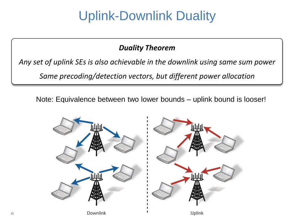
Uplink-Downlink Duality

Note: Equivalence between two lower bounds – uplink bound is looser!

21

Duality Theorem

Any set of uplink SEs is also achievable in the downlink using same sum power

Same precoding/detection vectors, but different power allocation

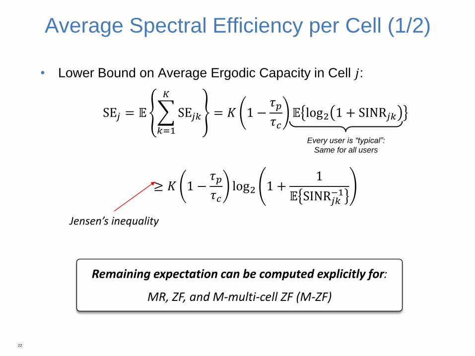
Average Spectral Efficiency per Cell (1/2)

• Lower Bound on Average Ergodic Capacity in Cell 𝑗:

SE𝑗 = 𝔼 SE𝑗𝑘

𝐾

𝑘=1

= 𝐾 1 −𝜏𝑝

𝜏𝑐𝔼 log2 1 + SINR𝑗𝑘

≥ 𝐾 1 −𝜏𝑝

𝜏𝑐log2 1 +

1

𝔼 SINR𝑗𝑘−1

Noise/Transmit Power

Every user is “typical”:

Same for all users

Jensen’s inequality

Remaining expectation can be computed explicitly for:

MR, ZF, and M-multi-cell ZF (M-ZF)

22

Average Spectral Efficiency per Cell (2/2)

• Lower Bound on Average Ergodic Capacity in Cell 𝑗:

SE𝑗 = 𝐾 1 −𝜏𝑝

𝜏𝑐log2 1 +

1

𝐼𝑗

• Interference term depends on processing:

23

Loss from pilots “SINR”

Noise/Transmit Power

𝐼𝑗MR = 𝜇𝑗𝑙

(2)+𝜇𝑗𝑙(2)

− (𝜇𝑗𝑙1)2

𝑀𝑙∈𝒫𝑗(𝑓)\{𝑗}

+ 𝜇𝑗𝑙

(1)𝐾 +

𝜎2

𝑝𝑙∈ℒ

𝑀 𝜇𝑗𝑙

(1)

𝑙∈𝒫𝑗 𝑓

+𝜎2

𝑝𝜏𝑝

𝐼𝑗ZF = 𝜇𝑗𝑙

(2)+𝜇𝑗𝑙(2)

− (𝜇𝑗𝑙1)2

𝑀 − 𝐾𝑙∈𝒫𝑗(𝑓)\{𝑗}

+ 𝜇𝑗𝑙

1𝐾 +

𝜎2

𝑝𝑙∈ℒ

𝑀 − 𝐾 𝜇𝑗𝑙

(1)

𝑙∈𝒫𝑗 𝑓

+𝜎2

𝑝𝜏𝑝−

𝜇𝑗𝑙1

2𝐾

𝑀 − 𝐾𝑙∈𝒫𝑗 𝑓

Interference from all cells Pilot contamination 1/(Estimation quality) Interference suppression

Only terms that remain as 𝑀 → ∞: Finite limit on SE

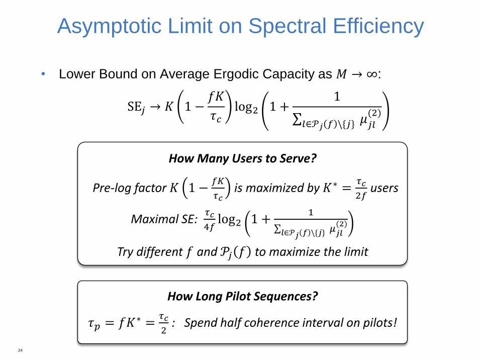
Asymptotic Limit on Spectral Efficiency

• Lower Bound on Average Ergodic Capacity as 𝑀 → ∞:

SE𝑗 → 𝐾 1 −𝑓𝐾

𝜏𝑐log2 1 +

1

𝜇𝑗𝑙(2)

𝑙∈𝒫𝑗 𝑓 \{𝑗}

24

How Long Pilot Sequences?

𝜏𝑝 = 𝑓𝐾∗ =𝜏𝑐

2 : Spend half coherence interval on pilots!

How Many Users to Serve?

Pre-log factor 𝐾 1 −𝑓𝐾

𝜏𝑐 is maximized by 𝐾∗ =

𝜏𝑐

2𝑓 users

Maximal SE: 𝜏𝑐

4𝑓log2 1 +

1

𝜇𝑗𝑙(2)

𝑙∈𝒫𝑗 𝑓 \{𝑗}

Try different 𝑓 and 𝒫𝑗 𝑓 to maximize the limit

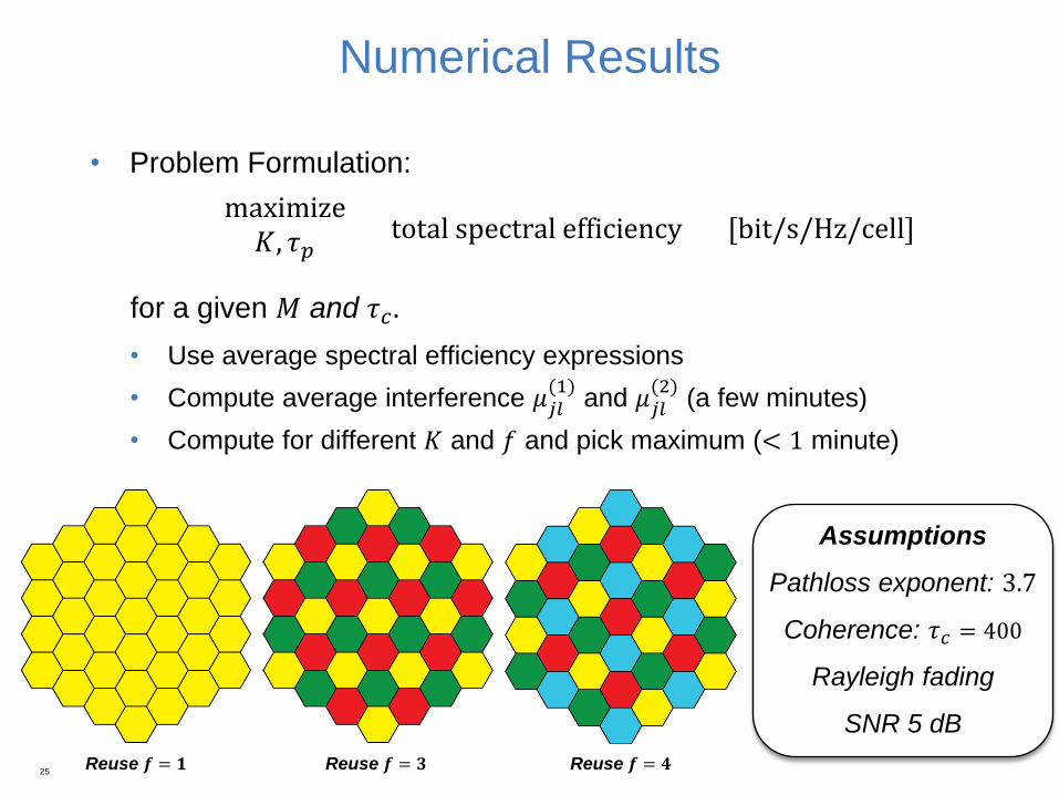
Numerical Results

• Problem Formulation:

maximize𝐾, 𝜏𝑝

total spectral efficiency [bit/s/Hz/cell]

for a given 𝑀 and 𝜏𝑐 .

• Use average spectral efficiency expressions

• Compute average interference 𝜇𝑗𝑙(1)

and 𝜇𝑗𝑙(2)

(a few minutes)

• Compute for different 𝐾 and 𝑓 and pick maximum (< 1 minute)

25 Reuse 𝒇 = 𝟏 Reuse 𝒇 = 𝟑 Reuse 𝒇 = 𝟒

Assumptions

Pathloss exponent: 3.7

Coherence: 𝜏𝑐 = 400

Rayleigh fading

SNR 5 dB

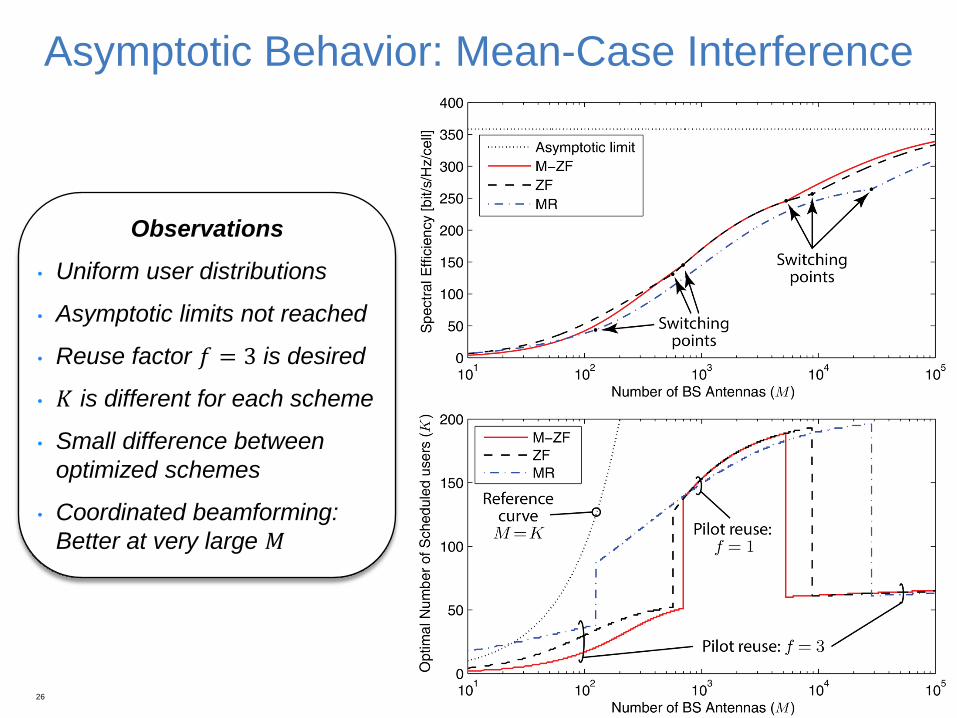
Asymptotic Behavior: Mean-Case Interference

26

Observations

• Uniform user distributions

• Asymptotic limits not reached

• Reuse factor 𝑓 = 3 is desired

• 𝐾 is different for each scheme

• Small difference between

optimized schemes

• Coordinated beamforming:

Better at very large 𝑀

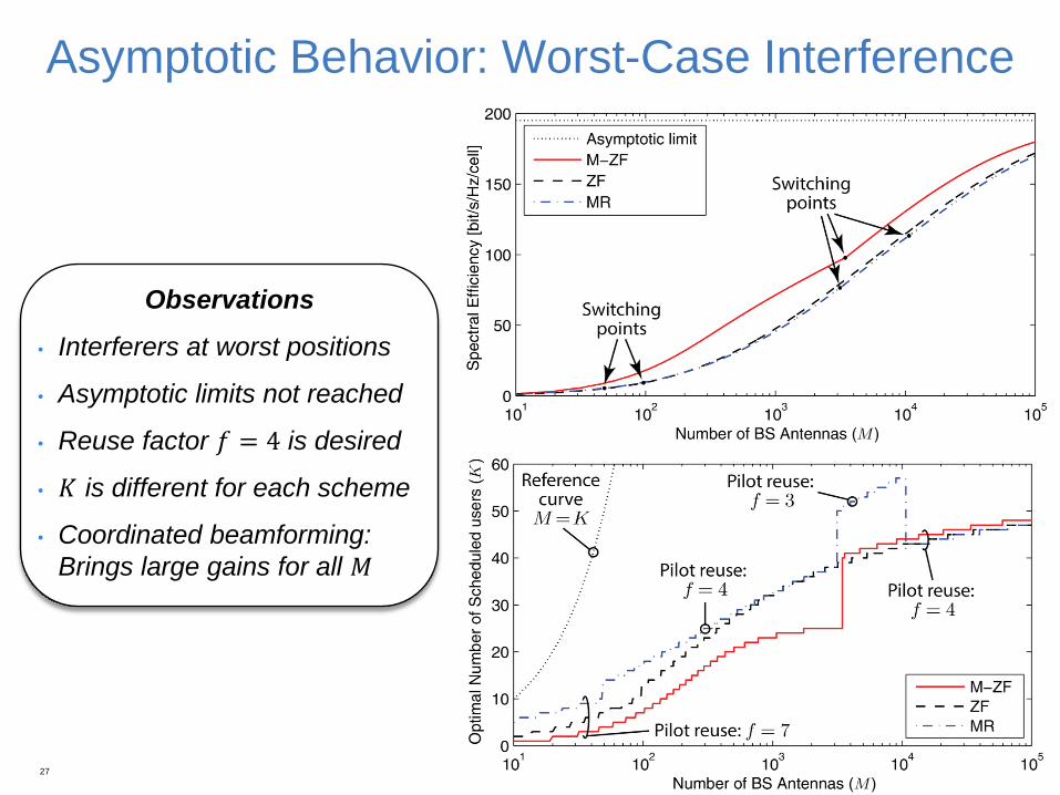
Asymptotic Behavior: Worst-Case Interference

27

Observations

• Interferers at worst positions

• Asymptotic limits not reached

• Reuse factor 𝑓 = 4 is desired

• 𝐾 is different for each scheme

• Coordinated beamforming:

Brings large gains for all 𝑀

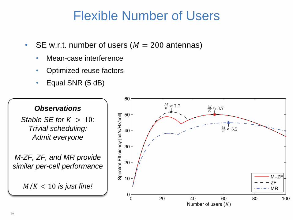
Flexible Number of Users

• SE w.r.t. number of users (𝑀 = 200 antennas)

• Mean-case interference

• Optimized reuse factors

• Equal SNR (5 dB)

28

Observations

Stable SE for 𝐾 > 10:

Trivial scheduling:

Admit everyone

M-ZF, ZF, and MR provide

similar per-cell performance

𝑀/𝐾 < 10 is just fine!

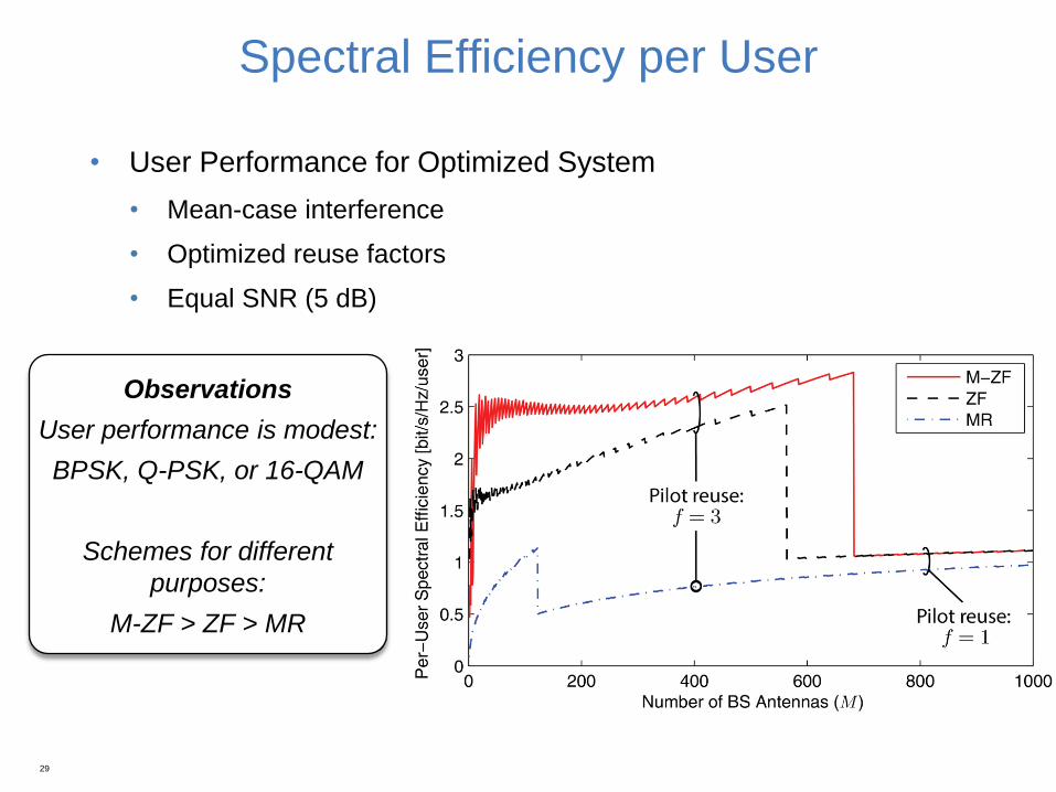
Spectral Efficiency per User

• User Performance for Optimized System

• Mean-case interference

• Optimized reuse factors

• Equal SNR (5 dB)

29

Observations

User performance is modest:

BPSK, Q-PSK, or 16-QAM

Schemes for different

purposes:

M-ZF > ZF > MR

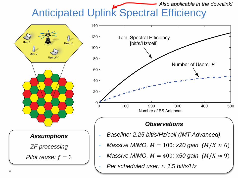
Anticipated Uplink Spectral Efficiency

30

Assumptions

ZF processing

Pilot reuse: 𝑓 = 3

Observations

• Baseline: 2.25 bit/s/Hz/cell (IMT-Advanced)

• Massive MIMO, 𝑀 = 100: x20 gain (𝑀/𝐾 ≈ 6)

• Massive MIMO, 𝑀 = 400: x50 gain (𝑀/𝐾 ≈ 9)

• Per scheduled user: ≈ 2.5 bit/s/Hz

Also applicable in the downlink!

Summary

• Massive MIMO delivers High Spectral Efficiency

• > 20x gains over IMT-Advanced are within reach

• Very high spectral efficiency per cell, not per user

• Non-universal pilot reuse (𝑓 = 3) is often preferred

• MR, ZF, M-ZF prefer different values on 𝐾 and 𝑓

• “An order of magnitude more antennas than users” is not needed

• Asymptotic limits

• Coherence interval (𝜏𝑐 symbols) limits multiplexing capability

• Allocate up to 𝜏𝑐/2 symbols for pilots

• We can handle very many users/cell – how many will there be?

31

Key References (1/2)

Seminal and Overview Papers

1. T. L. Marzetta, “Noncooperative Cellular Wireless with Unlimited Numbers of Base Station

Antennas,” IEEE Trans. Wireless Communications, 2010. IEEE W.R.G. Baker Prize Paper Award

2. J. Hoydis, S. ten Brink, M. Debbah, “Massive MIMO in the UL/DL of Cellular Networks: How Many

Antennas Do We Need?,” IEEE Journal on Selected Areas in Communications, 2013. IEEE

Leonard G. Abraham Prize

3. H. Q. Ngo, E. G. Larsson, and T. L. Marzetta, “Energy and Spectral Efficiency of Very Large

Multiuser MIMO Systems,” IEEE Trans. Commun., 2013. IEEE Stephen O. Rrice Prize

4. F. Rusek, D. Persson, B. K. Lau, E. G. Larsson, T. L. Marzetta, O. Edfors, and F. Tufvesson,

“Scaling up MIMO: Opportunities and Challenges with Very Large Arrays,” IEEE Signal Proces.

Mag., 2013.

5. J. Hoydis, K. Hosseini, S. ten Brink, and M. Debbah, “Making Smart Use of Excess Antennas:

Massive MIMO, Small Cells, and TDD,” Bell Labs Technical Journal, 2013.

6. E. G. Larsson, F. Tufvesson, O. Edfors, and T. L. Marzetta, “Massive MIMO for Next Generation

Wireless Systems,” IEEE Commun. Mag., 2014.

7. E. Björnson, E. Jorswieck, M. Debbah, B. Ottersten, “Multi-Objective Signal Processing

Optimization: The Way to Balance Conflicting Metrics in 5G Systems,” IEEE Signal Processing

Magazine, 2014.

8. T. L. Marzetta, “Massive MIMO: An Introduction,” Bell Labs Technical Journal, 2015

9. E. Björnson, E. G. Larsson, T. L. Marzetta, “Massive MIMO: 10 Myths and One Grand Question,”

IEEE Communications Magazine, To appear.

32

Key References (2/4)

Spectral Efficiency

1. J. Jose, A. Ashikhmin, T. L. Marzetta, and S. Vishwanath, “Pilot Contamination and Precoding in

Multi-cell TDD Systems,” IEEE Trans. Wireless Commun., 2011.

2. H. Huh, G. Caire, H. C. Papadopoulos, and S. A. Ramprashad, “Achieving ‘Massive MIMO’

Spectral Efficiency with a Not-so-Large Number of Antennas,” IEEE Trans. Wireless

Communications, 2012.

3. A. Adhikary, N. Junyoung, J.-Y. Ahn, G. Caire, “Joint Spatial Division and Multiplexing—The

Large-Scale Array Regime,” IEEE Trans. Information Theory, 2013.

4. E. Björnson and E. Jorswieck, “Optimal Resource Allocation in Coordinated Multi-cell Systems,”

Foundations and Trends in Communications and Information Theory, 2013.

5. H. Yang and T. Marzetta, “A Macro Cellular Wireless Network with Uniformly High User

Throughputs,” in Proc. IEEE VTC-Fall, 2014.

6. E. Björnson, E. G. Larsson, M. Debbah, “Massive MIMO for Maximal Spectral Efficiency: How

Many Users and Pilots Should Be Allocated?,” IEEE Trans. Wireless Communications, To

appear.

7. X. Li, E. Björnson, E. G. Larsson, S. Zhou, J. Wang, “Massive MIMO with Multi-cell MMSE

Processing: Exploiting All Pilots for Interference Suppression,” Submitted to IEEE Trans.

Wireless Communications.

33