peer influence background: long standing research interest in how our relations shape our attitudes...
TRANSCRIPT

Peer Influence
Background:•long standing research interest in how our relations shape our attitudes and behaviors.•One mechanism is that people, largely through conversation, change each others opinions•This implies that position in a communication network should be related to attitudes.
Freidkin & Cook:•A formal model of influence, based on communication
Cohen:•An application of a similar peer influence model relating to adolescent college aspirations
Topics Covered:•Basic Peer influence•Selection and influence•Dynamic mix of above•Dyad models

Friedkin & Cook
One piece in a long standing research program. Other cites include:
Friedkin, N. E. 1984. "Structural Cohesion and Equivalence Explanations of Social Homogeneity." Sociological Methods and Research 12:235-61.
———. 1998. A Structural Theory of Social Influence. Cambridge: Cambridge.
Friedkin, N. E. and E. C. Johnsen. 1990. "Social Influence and Opinions." Journal of Mathematical Sociology 15(193-205).
———. 1997. "Social Positions in Influence Networks." Social Networks 19:209-22.
See also the supplemental reading on the syllabus. Many particular context examples can be found as well.
Peer influence models assume that individuals’ opinions are formed in a process of interpersonal negotiation and adjustment of opinions.
•Can result in either consensus or disagreement•Looks at interaction among a system of actors•In this particular paper, look at the opinion results in an experimental setup.
Friedkin & Cook

Basic Peer Influence Model
Attitudes are a function of two sources:a) Individual characteristics
•Gender, Age, Race, Education, Etc. Standard sociology
b) Interpersonal influences•Actors negotiate opinions with others

Freidkin claims in his Structural Theory of Social Influence that the theory has four benefits:
•relaxes the simplifying assumption of actors who must either conform or deviate from a fixed consensus of others (public choice model)
•Does not necessarily result in consensus, but can have a stable pattern of disagreement
•Is a multi-level theory:•micro level: cognitive theory about how people weigh and combine other’s opinions•macro level: concerned with how social structural arrangements enter into and constrain the opinion-formation process
•Allows an analysis of the systemic consequences of social structures
Basic Peer Influence Model

Basic Peer Influence ModelFormal Model
XBY )1( (1)
)1()1()( )1( YWYY αα Tt (2)
Y(1) = an N x M matrix of initial opinions on M issues for N actors
X = an N x K matrix of K exogenous variable that affect YB = a K x M matrix of coefficients relating X to Y = a weight of the strength of endogenous interpersonal
influencesW = an N x N matrix of interpersonal influences

Basic Peer Influence ModelFormal Model
XBY )1( (1)
This is the standard sociology model for explaining anything: the General Linear Model.
It says that a dependent variable (Y) is some function (B) of a set of independent variables (X). At the individual level, the model says that:
k
kiki BXY
Usually, one of the X variables is , the model error term.

Basic Peer Influence Model
)1()1()( )1( YWYY αα Tt (2)
This part of the model taps social influence. It says that each person’s final opinion is a weighted average of their own initial opinions
)1()1( Yα
And the opinions of those they communicate with (which can include their own current opinions)
)1( TαWY

Basic Peer Influence Model
The key to the peer influence part of the model is W, a matrix of interpersonal weights. W is a function of the communication structure of the network, and is usually a transformation of the adjacency matrix. In general:
jij
ij
w
w
1
10
Various specifications of the model change the value of wii, the extent to which one weighs their own current opinion and the relative weight of alters.

Basic Peer Influence Model
1 2
3
4
1 2 3 41 1 1 1 02 1 1 1 03 1 1 1 14 0 0 1 1
1 2 3 41 .33 .33 .33 02 .33 .33 .33 03 .25 .25 .25 .254 0 0 .50 .50
1 2 3 41 .50 .25 .25 02 .25 .50 .25 03 .20 .20 .40 .204 0 0 .33 .67
Even
2*self
1 2 3 41 .50 .25 .25 02 .25 .50 .25 03 .17 .17 .50 .174 0 0 .50 .50
degree
Self weight:
1 2 3 41 2 1 1 02 1 2 1 03 1 1 2 14 0 0 1 2
1 2 3 41 2 1 1 02 1 2 1 03 1 1 3 14 0 0 1 1

Basic Peer Influence Model
)1()1()( )1( YWYY αα Tt
Formal Properties of the model
When interpersonal influence is complete, model reduces to:
)1(
)1()1()(
01
T
Tt
WY
YWYY
When interpersonal influence is absent, model reduces to:
)1(
)1()1()(
0
Y
YWYY
Tt
(2)

Basic Peer Influence Model
Formal Properties of the model
The model is directly related to spatial econometric models:
If we allow the model to run over t, we can describe the model as:
XBWYY )1()()( αα
XWYY~)()( α
Where the two coefficients ( and ) are estimated directly (See Doreian, 1982, SMR)

Basic Peer Influence ModelSimple example
1 2
3
4
1 2 3 41 .33 .33 .33 02 .33 .33 .33 03 .25 .25 .25 .254 0 0 .50 .50
Y1357
= .8
T: 0 1 2 3 4 5 6 7 1.00 2.60 2.81 2.93 2.98 3.00 3.01 3.01 3.00 3.00 3.21 3.33 3.38 3.40 3.41 3.41 5.00 4.20 4.20 4.16 4.14 4.14 4.13 4.13 7.00 6.20 5.56 5.30 5.18 5.13 5.11 5.10

Basic Peer Influence ModelSimple example
1 2
3
4
1 2 3 41 .33 .33 .33 02 .33 .33 .33 03 .25 .25 .25 .254 0 0 .50 .50
Y1357
= 1.0
1.00 3.00 3.33 3.56 3.68 3.74 3.78 3.813.00 3.00 3.33 3.56 3.68 3.74 3.78 3.815.00 4.00 4.00 3.92 3.88 3.86 3.85 3.847.00 6.00 5.00 4.50 4.21 4.05 3.95 3.90
T: 0 1 2 3 4 5 6 7

Basic Peer Influence ModelExtended example: building intuition
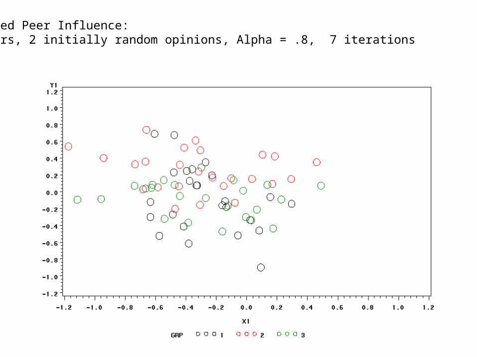
Consider a network with three cohesive groups, and an initially random distribution of opinions:
(to run this model, use peerinfl1.sas)

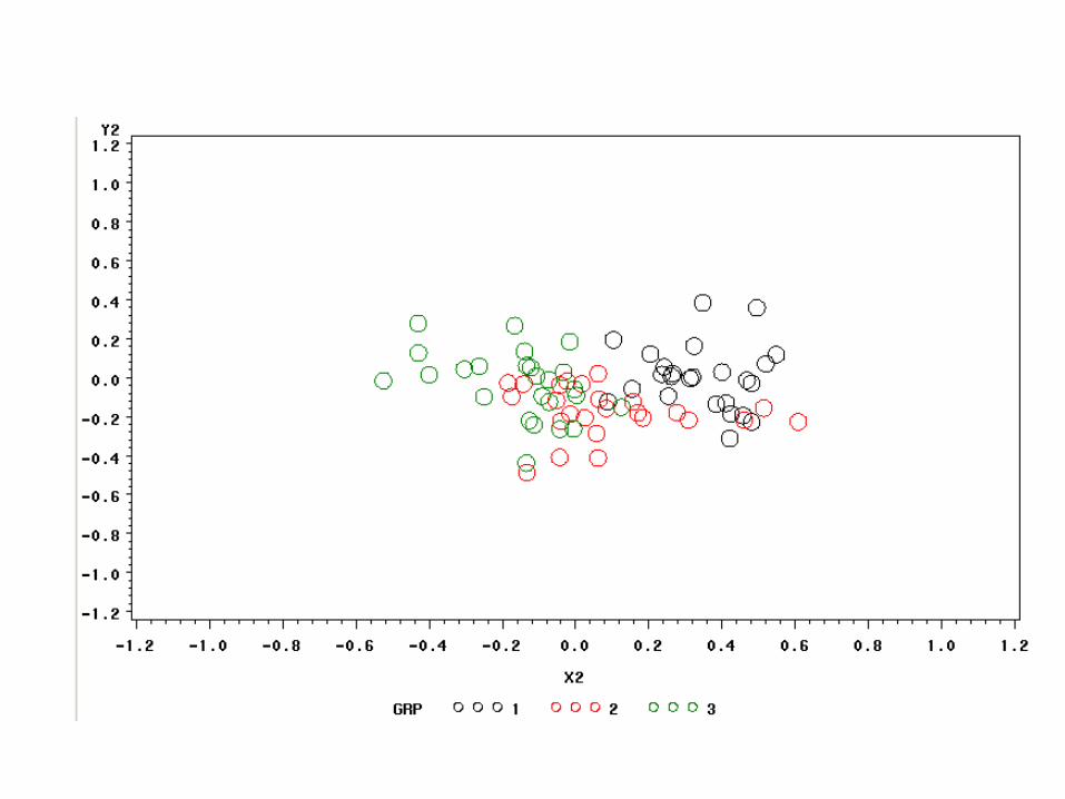
Simulated Peer Influence:75 actors, 2 initially random opinions, Alpha = .8, 7 iterations
Simulated Peer Influence:75 actors, 2 initially random opinions, Alpha = .8, 7 iterations

Simulated Peer Influence:75 actors, 2 initially random opinions, Alpha = .8, 7 iterations

Simulated Peer Influence:75 actors, 2 initially random opinions, Alpha = .8, 7 iterations

Simulated Peer Influence:75 actors, 2 initially random opinions, Alpha = .8, 7 iterations

Simulated Peer Influence:75 actors, 2 initially random opinions, Alpha = .8, 7 iterations

Simulated Peer Influence:75 actors, 2 initially random opinions, Alpha = .8, 7 iterations

Simulated Peer Influence:75 actors, 2 initially random opinions, Alpha = .8, 7 iterations

Basic Peer Influence ModelExtended example: building intuition
Consider a network with three cohesive groups, and an initially random distribution of opinions:
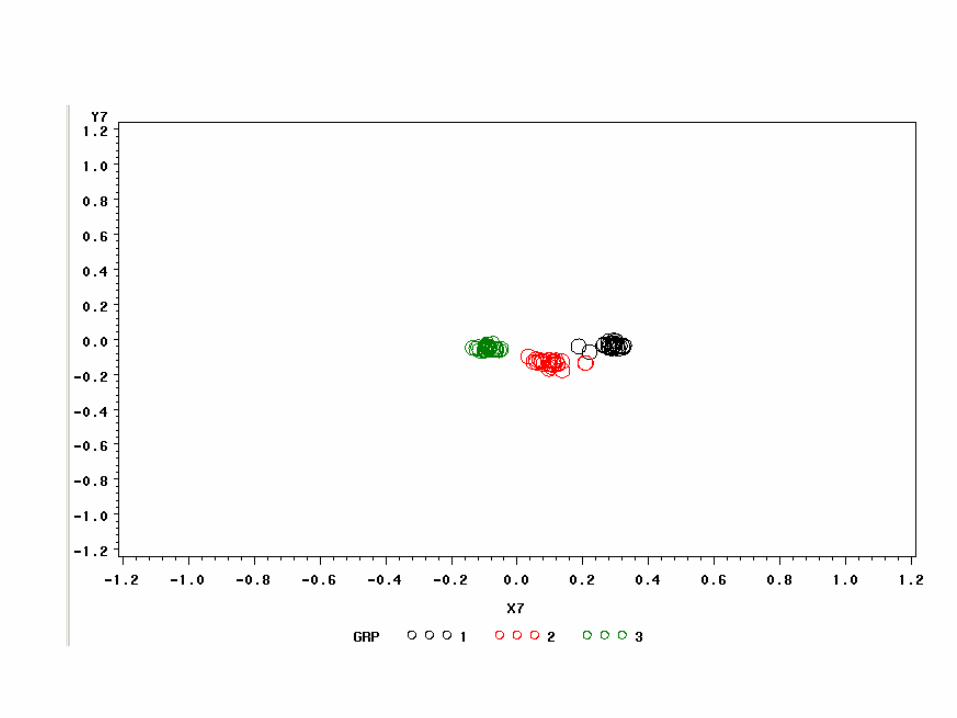
Now weight in-group ties higher than between group ties
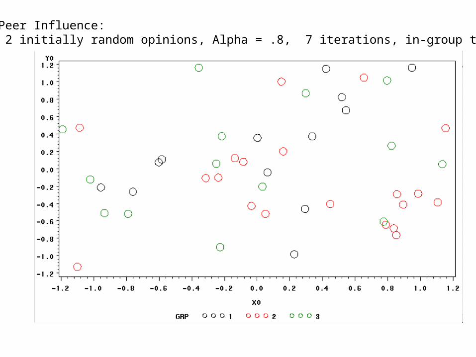
Simulated Peer Influence:75 actors, 2 initially random opinions, Alpha = .8, 7 iterations, in-group tie: 2


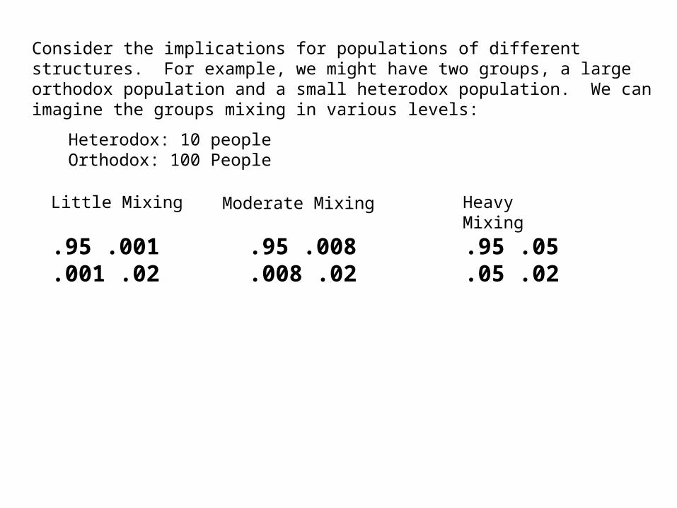
Consider the implications for populations of different structures. For example, we might have two groups, a large orthodox population and a small heterodox population. We can imagine the groups mixing in various levels:
Little Mixing Moderate Mixing Heavy Mixing
.95 .05 .05 .02
.95 .008 .008 .02
.95 .001 .001 .02
Heterodox: 10 peopleOrthodox: 100 People
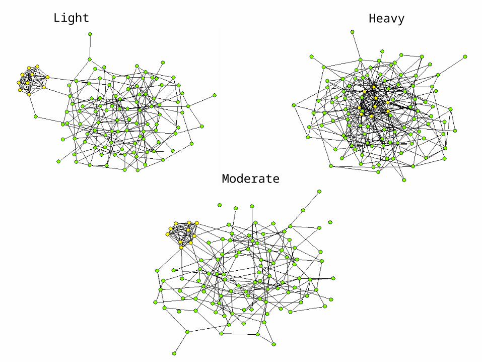
Light Heavy
Moderate

Light mixing

Light mixing

Light mixing

Light mixing

Light mixing

Light mixing

Moderate mixing

Moderate mixing

Moderate mixing

Moderate mixing

Moderate mixing
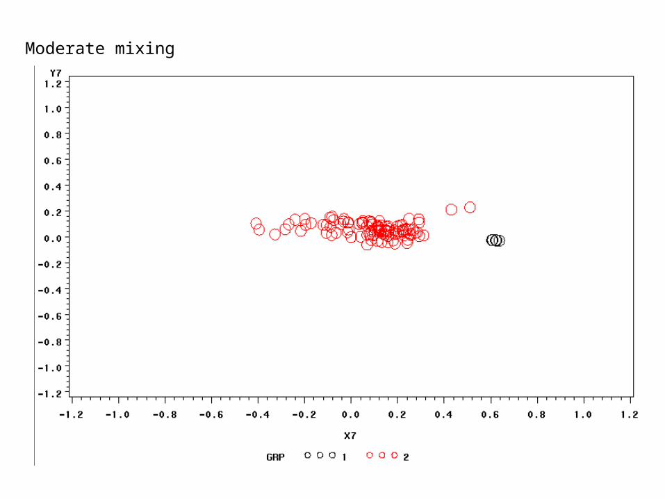
Moderate mixing

High mixing
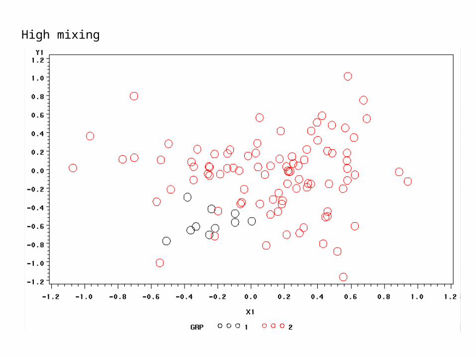
High mixing

High mixing

High mixing

High mixing

High mixing

In an unbalanced situation (small group vs large group) the extent of contact can easily overwhelm the small group. Applications of this idea are evident in:
•Missionary work (Must be certain to send missionaries out into the world with strong in-group contacts)•Overcoming deviant culture (I.e. youth gangs vs. adults)•Work by Hyojung Kim (U Washington) focuses on the first of these two processes in social movement models

In recent extensions (Friedkin, 1998), Friedkin generalizes the model so that alpha varies across people. We can extend the basic model by (1) simply changing to a vector (A), which then changes each person’s opinion directly, and (2) by linking the self weight (wii) to alpha.
)1()1()( )( YAIAWYY Tt
Were A is a diagonal matrix of endogenous weights, with 0 < aii < 1. A further restriction on the model sets wii = 1-aii
This leads to a great deal more flexibility in the theory, and some interesting insights. Consider the case of group opinion leaders with unchanging opinions (I.e. many people have high aii, while a few have low):

Group 1 Leaders
Group 2 Leaders
Group 3 Leaders
Peer Opinion Leaders
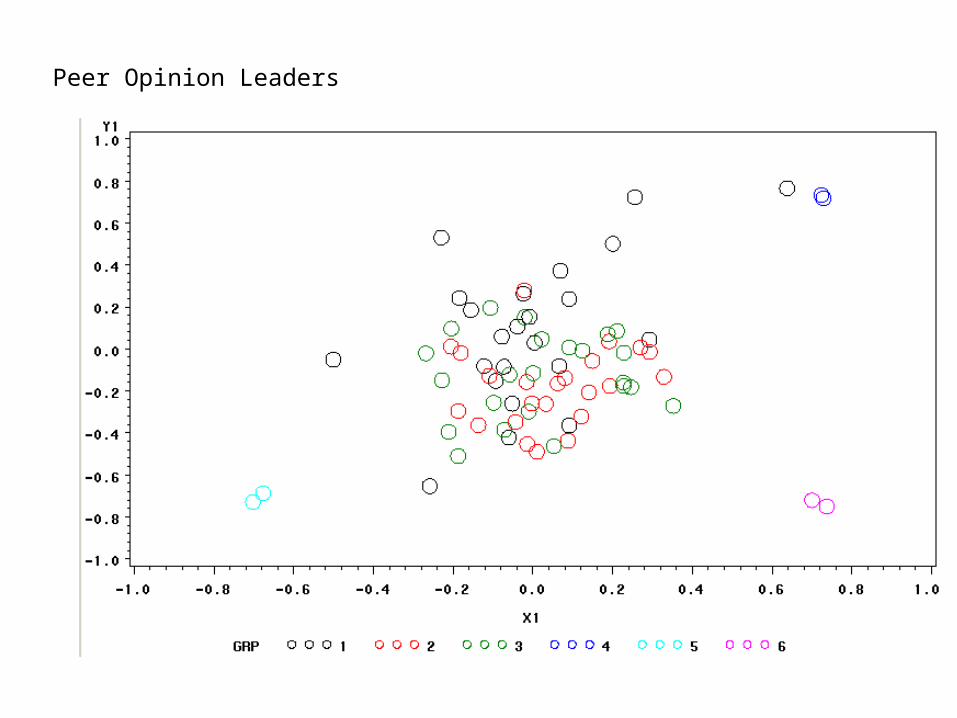
Peer Opinion Leaders
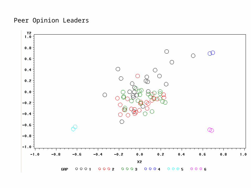
Peer Opinion Leaders

Peer Opinion Leaders

Peer Opinion Leaders
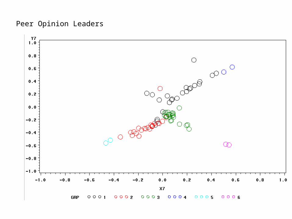
Peer Opinion Leaders

Further extensions of the model might:
•Time dependent : people likely value other’s opinions more early than later in a decision context
•Interact with XB: people’s self weights are a function of their behaviors & attributes
•Make W dependent on structure of the network (weight transitive ties greater than intransitive ties, for example)
•Time dependent W: The network of contacts does not remain constant, but is dynamic, meaning that influence likely moves unevenly through the network
•And others likely abound….

Testing the fit of the general model.Experimental results
In the Friedkin and Cook paper, they test a version of the general model experimentally in 50 4 person groups.
Each person was given time to form an initial opinion on a set of scenarios, and then discuss their opinions with others, based on a given structure.
Based on the model, they can predict the relation between people’s initial opinions and the group’s final opinion.
They find that the model does predict well, even controlling for the spread of initial opinions, the average opinion, and the structure of the network

Testing the fit of the general modelIdentifying peer influence in real data
There are two general ways to test for peer influence in an observed network. The first estimates the parameters ( and ) of the peer influence model directly, the second transforms the network into a dyadic model, predicting similarity among actors.
XWYY~)()( α
Peer influence model:For details, see Doriean, 1982, sociological methods and research. Also Roger Gould (AJS, Paris Commune paper for example)

XWYY~)()( α
Peer influence model:For details, see Doriean, 1982, sociological methods and research. Also Roger Gould (AJS, Paris Commune paper for example)
The basic model says that people’s opinions are a function of the opinions of others and their characteristics.
WY = A simple vector which can be added to your model. That is, multiple Y by a W matrix, and run the regression with WY as a new variable, and the regression coefficient is an estimate of .
This is what Doriean calls the QAD estimate of peer influence.

The problem with the above regression is that cases are, by definition, not independent. In fact, WY is also known as the ‘network autocorrelation’ coefficient, since a ‘peer influence’ effect is an autocorrelation effect -- your value is a function of the people you are connected to. In general, OLS is not the best way to estimate this equation. That is, QAD = Quick and Dirty, and your results will not be exact.In practice, the QAD approach (perhaps combined with a GLS estimator) results in empirical estimates that are “virtually indistinguishable” from MLE (Doreian et al, 1984)
The proper way to estimate the peer equation is to use maximum likelihood estimates, and Doreian gives the formulas for this in his paper.
The other way is to use non-parametric approaches, such as the Quadratic Assignment Procedure, to estimate the effects.

An empirical Example: Peer influence in the OSU Graduate Student Network.
(to run the model, see osupeerpi1.sas)
Each person was asked to rank their satisfaction with the program, which is the dependent variable in this analysis.
I constructed two W matrices, one from HELP the other from Best Friend. I treat relations as symmetric and valued, such that:
0
1
otherwise 0
1A and 1 if 2
1Aor 1 if 1
jitijt
jitijt
ii
jij
ijt
W
W
A
A
W
I also include Race (white/Non-white, Gender and Cohort Year as exogenous variables in the model.

An empirical Example: Peer influence in the OSU Graduate Student Network.
Distribution of Satisfaction with the department.

Parameter Estimates
Parameter StandardizedVariable Estimate Pr > |t| Estimate
Intercept 2.60252 0.0931 0FEMALE -1.07540 0.0142 -0.25455NONWHITE -0.22087 0.5975 -0.05491y00 0.93176 0.0798 0.21627y99 -0.19375 0.7052 -0.04586y98 -0.45912 0.4637 -0.08289y97 0.60670 0.3060 0.11919PEER_BF 0.23936 0.0002 0.42084PEER_H 0.50668 0.0277 0.23321
Model R2 = .41, compared to .15 without the peer effects

The most common method for estimating peer effects is to include the mean of ego’s alters in the network. Under certain specifications of the model, this is exactly the same as the QAD analysis sketched above.

Peer influence through Dyad Models
Another way to get at peer influence is not through the level of Y, but through the extent to which actors are similar with respect to Y. Recall the simulated example: peer influence is reflected in how close points are to each other.

Peer influence through Dyad Models
The model is now expressed at the dyad level as:
ijk
kkijij eXbAbbY 10
Where Y is a matrix of similarities, A is an adjacency matrix, and Xk is a matrix of similarities on attributes
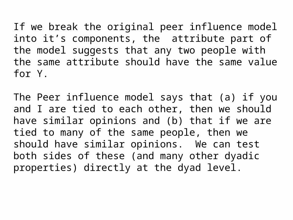
If we break the original peer influence model into it’s components, the attribute part of the model suggests that any two people with the same attribute should have the same value for Y.
The Peer influence model says that (a) if you and I are tied to each other, then we should have similar opinions and (b) that if we are tied to many of the same people, then we should have similar opinions. We can test both sides of these (and many other dyadic properties) directly at the dyad level.

NODE ADJMAT SAMERCE SAMESEX 1 0 1 1 1 0 0 0 0 0 0 1 0 0 1 0 0 0 1 0 0 1 1 0 0 1 1 0 2 1 0 1 0 0 0 1 0 0 1 0 0 0 1 0 0 0 1 0 0 0 0 1 1 0 0 1 3 1 1 0 0 1 0 1 0 0 0 0 0 1 0 1 1 1 0 1 0 0 1 0 0 1 1 0 4 1 0 0 0 1 0 0 0 0 0 0 1 0 0 1 1 1 0 1 0 1 0 0 0 1 1 0 5 0 0 1 1 0 1 0 1 0 1 1 0 0 0 0 0 0 1 0 1 0 0 0 1 0 0 1 6 0 0 0 0 1 0 0 1 1 0 0 1 1 0 0 1 1 0 0 1 0 0 1 0 0 0 1 7 0 1 1 0 0 0 0 0 0 0 0 1 1 0 1 0 1 0 1 0 1 1 0 0 0 1 0 8 0 0 0 0 1 1 0 0 1 0 0 1 1 0 1 1 0 0 1 0 1 1 0 0 1 0 0 9 0 0 0 0 0 1 0 1 0 1 1 0 0 1 0 0 0 0 0 1 0 0 1 1 0 0 0

Distance (Dij=abs(Yi-Yj).000 .277 .228 .181 .278 .298 .095 .307 .481.277 .000 .049 .096 .555 .575 .182 .584 .758.228 .049 .000 .047 .506 .526 .134 .535 .710.181 .096 .047 .000 .459 .479 .087 .488 .663.278 .555 .506 .459 .000 .020 .372 .029 .204.298 .575 .526 .479 .020 .000 .392 .009 .184.095 .182 .134 .087 .372 .392 .000 .401 .576.307 .584 .535 .488 .029 .009 .401 .000 .175.481 .758 .710 .663 .204 .184 .576 .175 .000
Y 0.32 0.59 0.54 0.50 0.04 0.02 0.41 0.01-0.17

Obs SENDER RCVER SIM NOM SAMERCE SAMESEX
1 1 2 0.27694 1 1 0 2 1 3 0.22828 1 0 1 3 1 4 0.18136 1 0 1 4 1 5 0.27766 0 1 0 5 1 6 0.29763 0 0 0 6 1 7 0.09473 0 0 1 7 1 8 0.30671 0 0 1 8 1 9 0.48148 0 1 0 9 2 1 0.27694 1 1 0 10 2 3 0.04866 1 0 0 11 2 4 0.09559 0 0 0 12 2 5 0.55460 0 1 1 13 2 6 0.57457 0 0 1 14 2 7 0.18221 1 0 0 15 2 8 0.58365 0 0 0

The REG Procedure Model: MODEL1 Dependent Variable: SIM
Analysis of Variance
Sum of MeanSource DF Squares Square F Value Pr > F
Model 4 0.90657 0.22664 9.29 <.0001Error 31 0.75591 0.02438Corrected Total 35 1.66248
Root MSE 0.15615 R-Square 0.5453 Dependent Mean 0.33161 Adj R-Sq 0.4866 Coeff Var 47.08929
Parameter Estimates
Parameter Standard Variable DF Estimate Error t Value Pr > |t|
Intercept 1 0.51931 0.05116 10.15 <.0001 NOM 1 -0.17054 0.05963 -2.86 0.0075 SAMERCE 1 0.05387 0.05916 0.91 0.3696 SAMESEX 1 -0.06535 0.05365 -1.22 0.2324 NCOMFND 1 -0.16134 0.03862 -4.18 0.0002

Like the basic Peer influence model, cases in a dyad model are not independent. However, the non-independence now comes from two sources: the fact that the same person is represented in (n-1) dyads and that i and j are linked through relations.
One of the best solutions to this problem is QAP: Quadratic Assignment Procedure. A non-parametric procedure for significance testing.
QAP runs the model of interest on the real data, then randomly permutes the rows/cols of the data matrix and estimates the model again. In so doing, it generates an empirical distribution of the coefficients.


Cohen: The problem of Selection and Influence
Well known that cohesive groups tend to be more similar (homogeneous) than the population at large. Why is this so? It may be due either to influence: people change as a function of the people around them or selection: people join groups based on their behaviors
Cohen re-analyzed data by Coleman on “Newlawn” a middle-class white suburban school of about 1000 students, and identified cliques of students in the school.
(His measure of clique is pretty exclusive: only 9% of the males and 40% of the females in the school fit his definition)
He proposes to answer the selection vs. influence question by looking at changes in behavior and changes in group composition over time.


Design:
Sf(F) = average std. Dev. Of fall members in the fall
Sf(S) = average std. Dev. Of spring members in the fall
Ss(F) = average std. Dev. Of Fall members in the Spring
Ss(S) = average std. Dev. Of Spring members in the Spring
Ss(S) - Sf(F) = change in group homogeneity over time. Not clear whether it is due to changes in behavior or changes in members
Ss(F) - Sf(F) = change in group homogeneity over time, for only those people who are in the same group both times. Removes the selection effect.

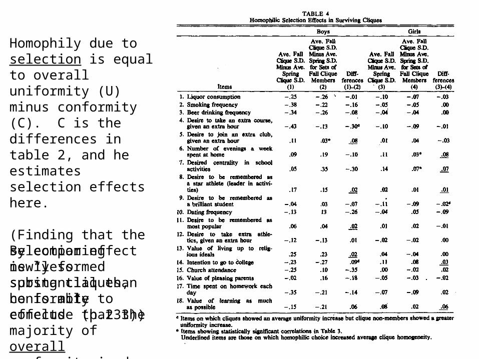
Homophily due to selection is equal to overall uniformity (U) minus conformity (C). C is the differences in table 2, and he estimates selection effects here.
(Finding that the selection effect is “less substantial than conformity effects” (p.233))
By comparing newly formed spring cliques, he is able to conclude that the majority of overall conformity is due to initial selection.

A mixed selection and influence model: Simultaneous balance on friendship and behavior.
Two linked models:a) actors seek interpersonal balance among friendsb) actors change their opinions / behaviors as a weighted function of the people they are tied to, with W weighted by number of transitive ties