performance characteristics of a retroreflector array
TRANSCRIPT
Naval Research Laboratory Washington, DC 20375-5320
NRLÄ/8120 -97-9875
Performance Characteristics of a Retroreflector Array Optimized for LEO Spacecraft
G. CHARMAINE GILBREATH
PETER B. ROLSMA
ROBERT KESSEL
ROBERT B. PATTERSON
JAMES A. GEORGES m
Advanced Systems Technology Branch Space Systems Development Department
December 31,1997
CO <£> 00 o
to o
o DTIC QUALITY INSPECTED t t-\
Approved for public release; distribution unlimited.

REPRODUCTION QUALITY NOTICE
This document is the best quality available. The copy furnished to DTIC contained pages that may have the foiiowing quality problems:
• Pages smaller or larger than normal.
• Pages with background color or light colored printing.
• Pages with small type or poor printing; and or
• Pages with continuous tone material or color photographs.
Due to various output media available these conditions may or may not cause poor legibility in the microfiche or hardcopy output you receive.
I/3I If this block is checked, the copy furnished to DTIC contained pages with color printing, that when reproduced in Black and White, may change detail of the original copy.

REPORT DOCUMENTATION PAGE Form Approved OMB No. 0704-0188
Public reporting burden for this collection of information is estimated to average 1 hour per response, including the time for reviewing instructions, searching existing data sources, gathering and maintaining the data needed, and completing and reviewing the collection of information. Send comments regarding this burden estimate or any other aspect of this collection of information, including suggestions for reducing this burden, to Washington Headquarters Services, Directorate for Information Operations and Reports, 1215 Jefferson Davis Highway, Suite 1204, Arlington, VA 22202-4302, and to the Office of Management and Budget. Paperwork Reduction Project (0704-0188), Washington, DC 20503.
1. AGENCY USE ONLY {Leave Blank) 2. REPORT DATE
December 31, 1997
3. REPORT TYPE AND DATES COVERED
Final Report
4. TITLE AND SUBTITLE
Performance Characteristics of a Retroreflector Array Optimized for LEO Spacecraft
5. FUNDING NUMBERS
6. AUTHOR(S)
G. Charmaine Gilbreath, Peter B. Rolsma, Robert Kessel, Robert B. Patterson and James A. Georges HI
7. PERFORMING ORGANIZATION NAME(S) AND ADDRESS(ES)
Naval Research Laboratory Washington, DC 20375-5320
8. PERFORMING ORGANIZATION REPORT NUMBER
NRL/FR/8120-97-9875
9. SPONSORING/MONITORING AGENCY NAME(S) AND ADDRESS(ES)
Space and Naval Warfare Systems Command SAP/FMBMB (AFOY) Washington, DC 20050-6335
10. SPONSORING/MONITORING AGENCY REPORT NUMBER
11. SUPPLEMENTARY NOTES
12a. DISTRIBUTION/AVAILABILITY STATEMENT
Approved for public release; distribution unlimited.
12b. DISTRIBUTION CODE
13. ABSTRACT [Maximum 200 words)
This report presents a predicted link analysis for the operational characteristics of a retroreflector array designed, built, and space-qualified by the Naval Research Laboratory for Low Earth Orbiting spacecraft. The predictions rest on the combination of numerical analysis and direct laboratory measurements of the retroreflector array's optical properties. The report also describes the assumptions we used for link analysis as they pertain to passes over Midway Research Center. The report includes a description and photo of the array itself, as well as the test and levels used to space qualify the array.
14. SUBJECT TERMS
Satellite laser ranging Retroreflector SLR Orbit determination
Retroreflectors
15. NUMBER OF PAGES
70
16. PRICE CODE
17. SECURITY CLASSIFICATION OF REPORT
UNCLASSIFIED
18. SECURITY CLASSIFICATION OF THIS PAGE
UNCLASSIFIED
19. SECURITY CLASSIFICATION OF ABSTRACT
UNCLASSIFIED
20. LIMITATION OF ABSTRACT
UL
NSN 7540-01-280-5500
DTIC QUALITY INSPECTED 3
Standard Form 298 (Rev. 2-89) Prescribed by ANSI Std 239-18
298-102
CONTENTS
EXECUTIVE SUMMARY E-l
1 INTRODUCTION 1
2 SATELLITE LASER RANGING SYSTEM CHARACTERISTICS 2
2.1 Return Pulse Detection and System Trade-offs 3 2.2 Ground Station Specifications and LEO Orbit Characteristics 4 2.3 Target Diffraction Effects and CTLRCS 5 2.4 Satellite Velocity Aberration 6
3 NRL LEO RETROREFLECTOR ARRAY 7
4 NUMERICAL COMPUTATION OF SATELLITE LASER RANGING PERFORMANCE 8
4.1 Single Circular Retroreflector Far Field Diffraction Patterns and <TLRCS 8 4.1.1 Normal Incidence 8 4.1.2 Off-axis Incidence 10 4.1.3 Bevel Losses 12
4.2 Retroreflector Array Far Field Diffraction Patterns and CXRCS 15 4.3 Computation of Orbital Performance 16
5 PREDICTED ORBITAL PERFORMANCE 16
5.1 NRL LEO Array Performance in Orbit 16 5.2 NRL LEO Array and Single Retroreflector Performance Comparison 20 5.3 Optical Phase Center and Timing Precision 23 5.4 Further Comparison of Single Retroreflectors and Retroreflector Arrays 26
6 EXPERIMENTAL DETERMINATION OF aLRCs 28
6.1 Procedure 28 6.2 Calibration 29
6.2.1 Spatial Calibration 29 6.2.2 Radiometrie Intensity Calibration 29
6.3 Results and Comparison to Numerical Computation 30
7 SPACE QUALIFICATION OF THE NRL LEO RETROREFLECTOR ARRAY 33
7.1 Random Vibration Tests 33 7.2 Thermal Vacuum Tests 34 7.3 Pyroshock Tests 34
iii
IV Gilbreath, Rolsma, Kessel, Patterson, and Georges
8 CONCLUSIONS 34
ACKNOWLEDGMENTS 34
ACRONYMS 35
REFERENCES 35
Appendix A - DIFFRACTION PATTERN AND PASS GEOMETRY CALCULATIONS 37
A.l Circular Retrorefiector Far Field Diffraction Patterns 37 A.2 Converting Pass Geometry to kxky Space 43
Appendix B - SCILAB LISTINGS 46
B.l Circular Retrorefiector Directly Overhead Without Bevels 46 B.2 Circular Retrorefiector Off Normal Incidence Without Bevels 46 B.3 Circular Retrorefiector Off Normal Incidence With Bevels 47 B.4 Conversion to kxky 49
Appendix C - SPACECRAFT ENGINEERING DEPARTMENT SPACE QUALIFICATION REPORT 53
C.l Test Report for the Retrorefiector Array 53 C.2 Test Procedure for the Retrorefiector Array 57 C.3 Final Acceptance Test Report of the Retrorefiector Array 58
EXECUTIVE SUMMARY
This report presents a full characterization of an optical retroreflector array designed for use with satellite laser ranging on low Earth orbit (LEO) spacecraft. The array was designed to provide a robust optical link from spacecraft in a circular orbit of about 1,100 km using typical NASA-like ground stations, including the small transportable laser ranging systems. The array will provide unambiguous returns for elevation angles above 20° for daytime and nighttime ranging. Consistent with requirements for precision position estimation, the optical configuration will provide phase errors no greater than those equivalent to a centimeter in ranging errors. The nominal site location for the analysis was Midway Research Center (MRC) in Quantico, Virginia.
Based on the analysis and experimental verification presented in this report, we show that the NRL LEO retroreflector array will meet these operational bounds well within margin. Furthermore, the array will also close a link for a system as modest as the field-transportable laser radar station (FTLRS) 13-cm aperture system on Capraia Island off the Tuscan coast. This latter analysis supports the potential of configuring a compact, transportable laser radar to obtain sub-meter, near real-time, satellite ephemerides.
In the course of the analysis and design, a suite of tools was developed to analyze performance for single cubes and retroreflector arrays of any size and configuration. The tools include numerical models that predict a given configuration's optical characteristics in terms of laser radar cross section (LRCS or CLRCS)- A second part of the tool set combines LRCS with ground station characteristics, atmospheric properties, and orbit dynamics to yield the numbers of both photons and photoelectrons for a given orbit over a specific ground site.
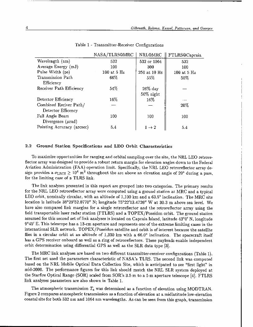
The array itself is compact and lightweight; it employs 22 1-cm retroreflectors mounted on a hemisphere to provide a CTLRCS °f greater than 104 m2 for all elevation angles above 20° with 108° field of view (FOV). It weighs 221 grams and measures 82 mm in diameter by 43 mm in height.
Analysis was verified experimentally by using a compact far field test bed. Comparison showed good agreement between the array's numerically modeled and measured optical characteristics. Manufacturing defects in the wave front quality of the retroreflectors direct energy to a slight extent into sidelobes (less than 2%). This redirection of energy into the sidelobes actually improves the link's performance by providing some compensation for velocity aberration.
Results were compared to the predicted performance of a single retroreflector. The comparison showed that the FOV would be severely restricted by using the single retroreflector, hence, orbital sampling would be significantly reduced. The number of passes as a function of elevation over a LEO ground repeat track is shown and illustrates quantitatively how limiting FOV in this manner impacts pass yield.
Predicted performance in the near-infrared at 1064 nm is also presented. Advantages of this wavelength include better transmission through the atmosphere and covertness due to transmission in the nonvisible region of the spectrum.
The array was space-qualified and testing specifications are given in Appendix C.
E-l
PERFORMANCE CHARACTERISTICS OF A RETROREFLECTOR ARRAY OPTIMIZED FOR LEO SPACECRAFT
1 INTRODUCTION
This report presents a full characterization of an optical retroreflector array designed for use with satellite laser ranging (SLR) on low Earth orbit (LEO) spacecraft. The array was designed to provide a robust optical link from a spacecraft in a circular orbit of about 1,100 km using typical NASA-like ground stations, including a small transportable laser ranging system (TLRS). The optical configuration was to provide phase errors no greater than those equivalent to a centimeter in ranging errors. The nominal site location for the analysis was Midway Research Center (MRC) in Quantico, Virginia.
Satellite laser ranging provides a powerful data type for precise orbit determination. Position estimation based on direct detection SLR can have performance comparable to a differential global positioning system (GPS) estimation and is used as the referenced "truth" by the scientific com- munity for geoscience and navigation. Although SLR data can generate a highly precise orbit estimator, it is weather-dependent. Therefore, this data type is uniquely suited for independent system performance validation of onboard spacecraft systems and for periodic calibration [1].
Significant information given in this report includes:
1. Link analyses providing the expected on-orbit performance of the NRL LEO array for two different ground site telescope configurations at MRC;
2. Link analyses of a single retroreflector and the NRL LEO array for a TOPEX/Poseidon pass over the Tuscan island of Capraia using a 13-cm aperture SLR system;
3. Supporting analyses including the direct numerical computation of a single retroreflector and the NRL LEO array's optical properties;
4. Pass yield as a function of elevation angle and the impact of field of view (FOV);
5. Laboratory measurements of the array's optical properties that validate numerical analyses; and
6. Space qualification results of the array's mechanical properties.
The report opens with a review of SLR systems establishing general terminology. As part of the review, the specific assumptions relevant to the link analyses are stated in Section 2.2. Section 3 describes the basic mechanical properties of the array. Section 4 covers the numerical computations required in the link analyses; notably, Section 4.1 considers single retroreflector optical properties and Section 4.2 extends the methods for a retroreflector array. The core results of this report are the on-orbit performance predictions in Section 5. In Section 6, the report presents experimental
Manuscript approved November 25, 1997
Gilbreatk, Rolsma, Kessel, Patterson, and Georges
Collimated Transmit Pulse
2
ATC = corrected time difference Diffracted Return Pulse
Central Maximum
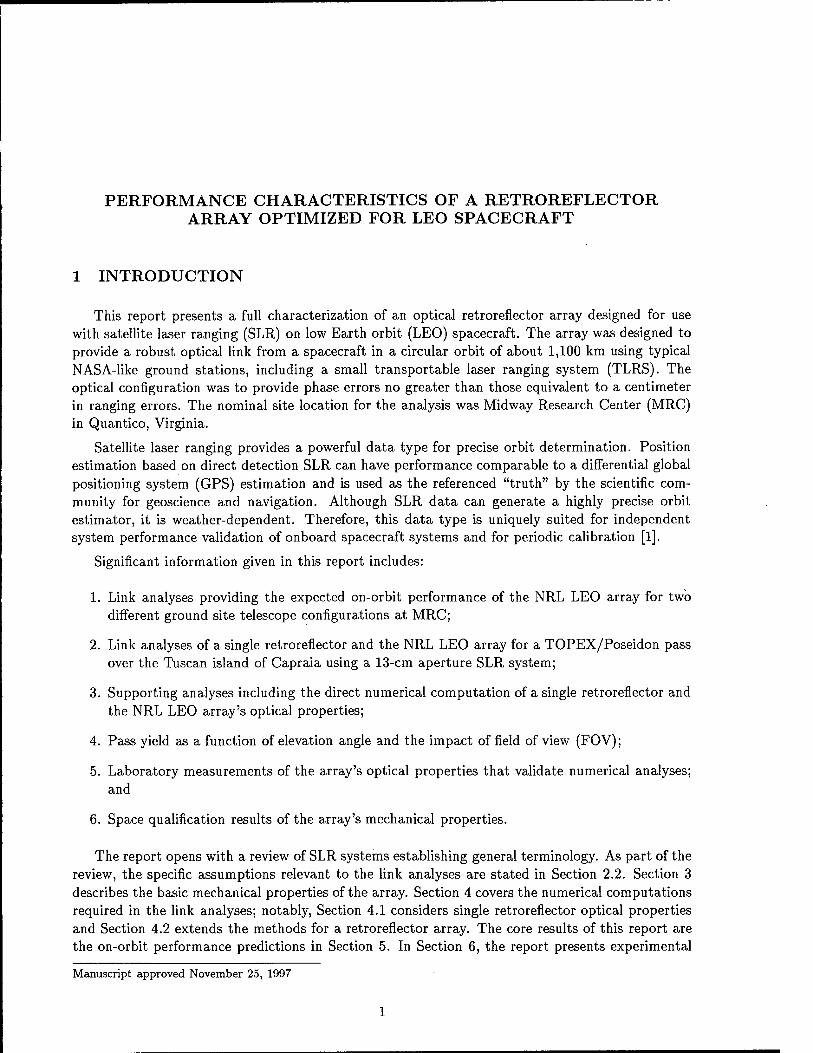
Fig. 1 - Satellite laser ranging (SLR) illustrating time-tagged round trip time of flight of the optical pulses used to
determine range to spacecraft. The intensity distribution on the ground is the far field diffraction pattern generated
by the size and shape of the target's aperture. The satellite's apparent orbital velocity determines the offset between
the central maximum of the diffraction pattern and the ground station.
results that validate the numerical models for optical properties. Section 7 summarizes the space qualification testing of the retroreflector array; Section 8 is the conclusion. Three appendices follow that cover the analytic details of the numerical methods, the full space qualification report, and source code listings. An acronym list is provide at the end of the main text.
2 SATELLITE LASER RANGING SYSTEM CHARACTERISTICS
In the context of this report, satellite laser ranging is direct-detection radar in the optical wavelength regime. When an orbit is properly sampled with a well-calibrated SLR data acquisition system, residuals and accuracies on the order of centimeters are routinely obtained [2].
Figure 1 illustrates basic aspects of the technique. Time-tagged time-of-flight differences are recorded, corrected for system delays, and converted to ranges. These ranges then provide input to an orbit determination model that is used to generate a three-dimensional estimate of the spacecraft's orbit and position.
LEO SLR Target Characteristics
2.1 Return Pulse Detection and System Trade-ofFs
The number of photoelectrons generated by an SLR system is given by the laser radar link
equation
Npe = rjDE0 (^) VTGTVLRCS (4^2) ARmT2aT
2c . (1)
The factors in Eq. (1) are:
T)D detector quantum efficiency &LRCS laser radar cross section £b transmit energy R slant range A wavelength AR receiver telescope area h Planck's constant T}R receiver efficiency c speed of light Ta one-way atmospheric transmission rjT transmission efficiency Tc one-way cirrus cloud transmission GT transmitter gain
A requirement of iVpe > 10 is a conservative standard for link closure and is used in this report. Although transfer efficiencies along telescope optical paths have been relatively stable over the last few decades, detector efficiency continues to improve. Consequently, it is useful to have the return pulse photons reaching the detector N-, as a system figure of merit:
iV7 Npe
VD
= Eo(
The link closure requirement for photons is iV7 > 100. Equation (2) depends on the telescope aperture AR. If the photon flux itself is needed for ground station trade studies, it is given by
flUX7 = -^l_ . (3) ARTIRVD
Based on the ground station specification in Section 2.2, the results of this report are given in terms of iVpe and iV7 for a 28-cm aperture and a 1-m aperture, as well as a 13-cm aperture for an extreme limiting case.
The factors in Eq. (1) determine the SLR trade-space and can be grouped into four categories: transfer efficiencies, transmitted pulse magnitude, environmental/orbit parameters, and geometric factors. The three transfer efficiencies, TJD, TJT, and TJR, are fixed by the technology of the ground
station. The initial number of photons, EQ \T^\, is determined by the laser source. The three
environmental/orbital parameters in Eq. (1), R, Ta, and Tc, are usually fixed boundary conditions beyond the experimenters' control. Two of the geometric factors, GT and AR, are associated with transmitting and receiving the laser ranging pulse at the ground station. For a Gaussian beam profile, the transmitter gain is
GT = I ° ] c-2(«point/*T)2 f (4)
where 0T is the divergence half-angle and 0point is the pointing uncertainty. The remaining geometric factor, CTLRCS) is determined by the SLR target and is a primary focus of this report's analyses. It is this factor that can most effectively compensate for the range loss that goes as R~4. Degnan's review [2] provides an extended treatment of each of the parameters in Eq. (1).
Gilbreath, Rolsma, Kessel, Patterson, and Georges
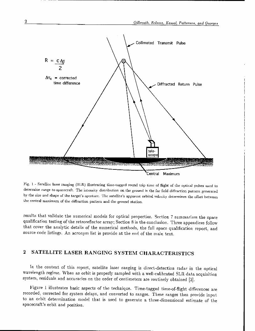
Table 1 - Transmitter-Receiver Configurations
NASA/TLRS@MRC NRL@MRC FTLRS@Capraia Wavelength (nm) 532 532 or 1064 532 Average Energy (mJ) 100 300 100 Pulse Width (ps) 100 at 5 Hz 250 at 10 Hz 100 at 5 Hz Transmission Path 66% 55% 50%
Efficiency Receiver Path Efficiency 54% 26% day
50% night —
Detector Efficiency 16% 16% — Combined Reciver Path/ — — 20%
Detector Efficency Full Angle Beam 100 100 100
Divergence (/xrad) Pointing Accuracy (arcsec) 5.4 l->2 5.4
2.2 Ground Station Specifications and LEO Orbit Characteristics
To maximize opportunities for ranging and orbital sampling over the site, the NRL LEO retrore- flector array was designed to provide a robust return margin for elevation angles down to the Federal Aviation Administration (FAA) operation limit. Specifically, the NRL LEO retroreflector array de- sign provides a CTLRCS > 104 m2 throughout the arc above an elevation angle of 20° during a pass, for the limiting case of a TLRS link.
The link analyses presented in this report are grouped into two categories. The primary results for the NRL LEO retroreflector array were computed using a ground station at MRC and a typical LEO orbit, nominally circular, with an altitude of 1,100 km and a 63.5° inclination. The MRC site location is latitude 38°29'52.0770" N; longitude 75°22'13.4726" W at 30.3 m above sea level. We have also compared link margins for a single retroreflector and the retroreflector array using the field transportable laser radar station (FTLRS) and a TOPEX/Poseidon orbit. The ground station assumed for this second set of link analyses is located on Capraia Island, latitude 43°0' N, longitude 9°45' E. This telescope has a 13-cm aperture and represents one of the extreme limiting cases in the international SLR network. TOPEX/Poseidon satellite and orbit is of interest because the satellite flies in a circular orbit at an altitude of 1,330 km with a 66.0° inclination. The spacecraft itself has a GPS receiver onboard as well as a ring of retroreflectors. These payloads enable independent orbit determination using differential GPS as well as the SLR data type [3].
The MRC link analyses are based on two different transmitter-receiver configurations (Table 1). The first set used the parameters characteristic of NASA's TLRS. The second link was computed based on the NRL Mobile Optical Data Collection Site, which is anticipated to see "first light" in mid-2000. The performance figures for this link should match the NRL SLR system deployed at the Starfire Optical Range (SOR) scaled from SOR's 3.5 m to a 1-m aperture telescope [4]. FTLRS link analyses parameters are also shown in Table 1.
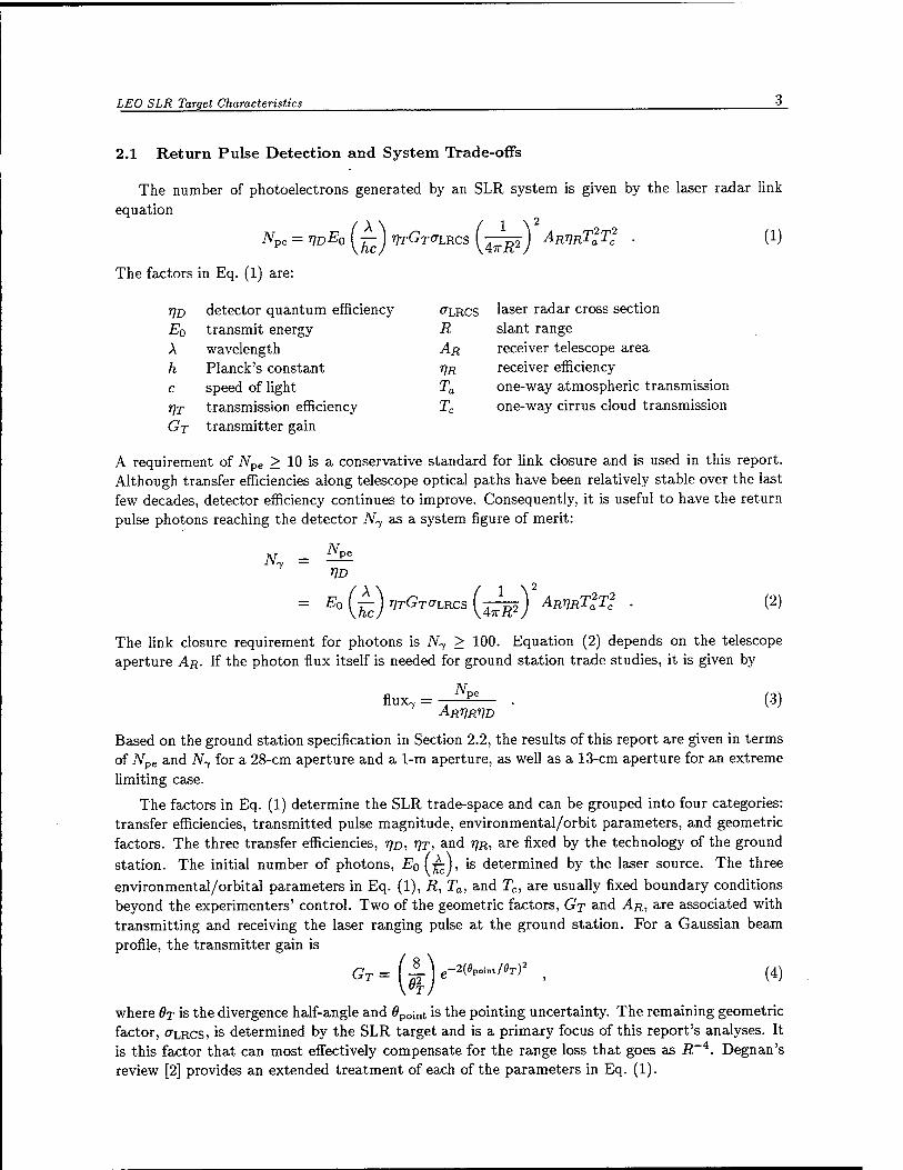
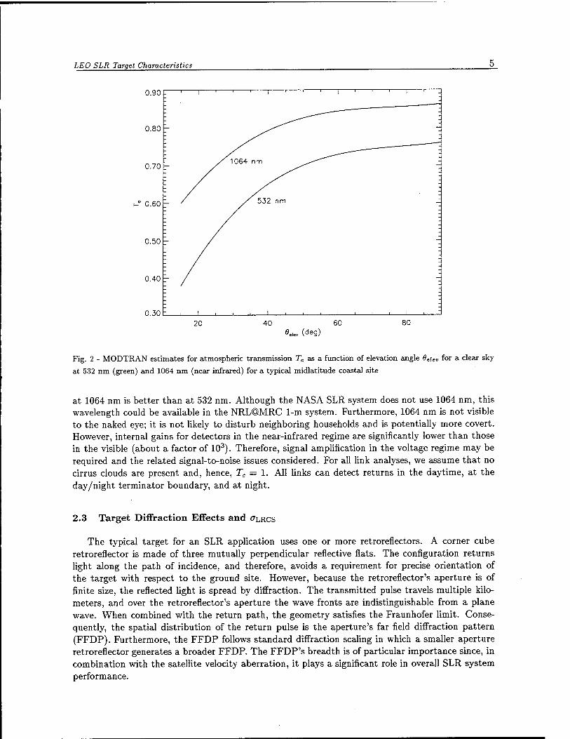
The atmospheric transmission Ta was determined as a function of elevation using MODTRAN. Figure 2 compares atmospheric transmission as a function of elevation at a midlatitude low-elevation coastal site for both 532 nm and 1064 nm wavelengths. As can be seen from this graph, transmission
LEO SLR Target Characteristics
0.90
0.80 -
0.70 r
0.60
0.50 -
0.40 -
0.30
(deg)
Fig. 2 - MODTRAN estimates for atmospheric transmission Ta as a function of elevation angle 9euv for a clear sky
at 532 nm (green) and 1064 nm (near infrared) for a typical midlatitude coastal site
at 1064 nm is better than at 532 nm. Although the NASA SLR system does not use 1064 nm, this wavelength could be available in the NRL@MRC 1-m system. Furthermore, 1064 nm is not visible to the naked eye; it is not likely to disturb neighboring households and is potentially more covert. However, internal gains for detectors in the near-infrared regime are significantly lower than those in the visible (about a factor of 103). Therefore, signal amplification in the voltage regime may be required and the related signal-to-noise issues considered. For all link analyses, we assume that no cirrus clouds are present and, hence, Tc — 1. All links can detect returns in the daytime, at the day/night terminator boundary, and at night.
2.3 Target Diffraction Effects and CTLRCS
The typical target for an SLR application uses one or more retroreflectors. A corner cube retroreflector is made of three mutually perpendicular reflective flats. The configuration returns light along the path of incidence, and therefore, avoids a requirement for precise orientation of the target with respect to the ground site. However, because the retroreflector's aperture is of finite size, the reflected light is spread by diffraction. The transmitted pulse travels multiple kilo- meters, and over the retroreflector's aperture the wave fronts are indistinguishable from a plane wave. When combined with the return path, the geometry satisfies the Fraunhofer limit. Conse- quently, the spatial distribution of the return pulse is the aperture's far field diffraction pattern (FFDP). Furthermore, the FFDP follows standard diffraction scaling in which a smaller aperture retroreflector generates a broader FFDP. The FFDP's breadth is of particular importance since, in combination with the satellite velocity aberration, it plays a significant role in overall SLR system performance.
Gilbreath, Rolsma, Kessel, Patterson, and Georges
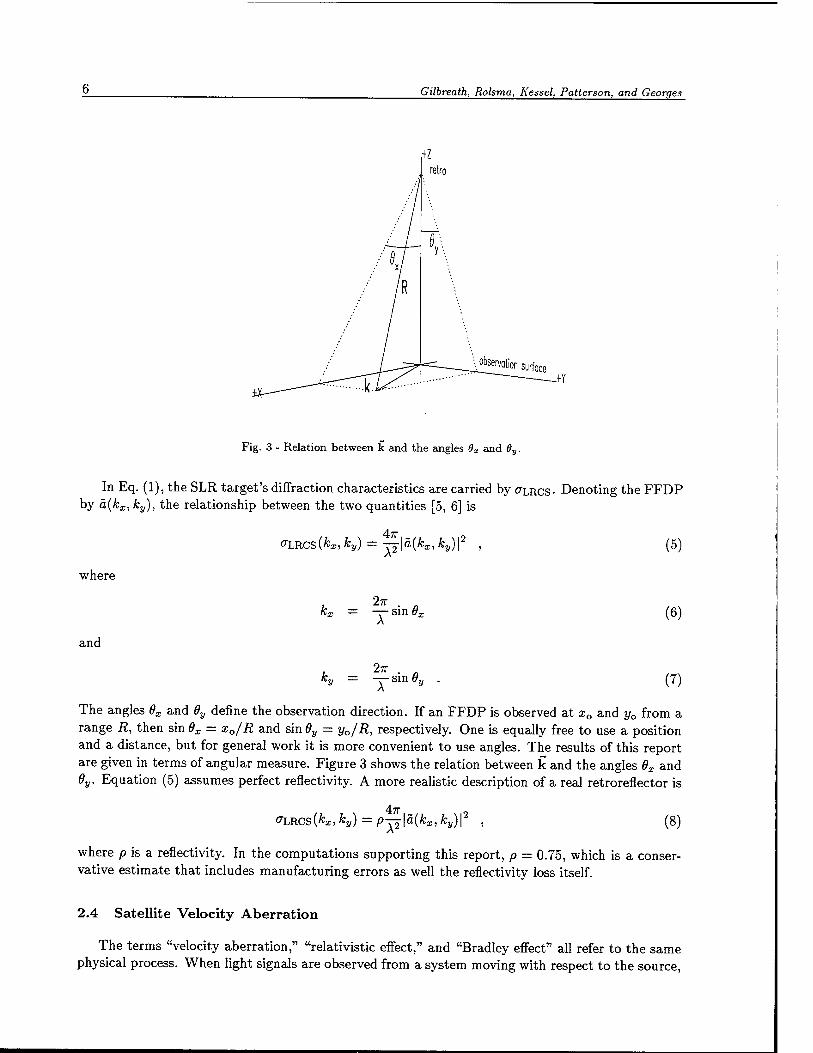
Fig. 3 - Relation between k and the angles 8X and 8y.
In Eq. (1), the SLR target's diffraction characteristics are carried by CTLRCS- Denoting the FFDP by ä(kx, ky), the relationship between the two quantities [5, 6] is
47T,
where
and
VLRCs{kx,ky) = -r-^\ä(kx, ky)
2TT kx = -r sin 6X
2n . „ ky = — sin 8y
(5)
(6)
(7)
The angles 9X and 6y define the observation direction. If an FFDP is observed at x0 and y0 from a range R, then sin 9X = x0/R and sin 0y = y0/R, respectively. One is equally free to use a position and a distance, but for general work it is more convenient to use angles. The results of this report are given in terms of angular measure. Figure 3 shows the relation between k and the angles 6X and 6y. Equation (5) assumes perfect reflectivity. A more realistic description of a real retroreflector is
47T, O-LRCS(^) ky) = p—\a(kx, ky)\ (8)
where p is a reflectivity. In the computations supporting this report, p = 0.75, which is a conser- vative estimate that includes manufacturing errors as well the reflectivity loss itself.
2.4 Satellite Velocity Aberration
The terms "velocity aberration," "relativistic effect," and "Bradley effect" all refer to the same physical process. When light signals are observed from a system moving with respect to the source,
LEO SLR Target Characteristics
<^-," <p!f . v'sV^-. rf^ :'P %,\
/ X iSSg^H^- Jl ' \* *
• i " ( 7<^H Jr!""-\ ML ■ V ''jl |^'-^tj
- ^ 1^^»§2? !;| P * |J '■ {^m^:] —
* '\ \Z>k ,jk\-*£r • * '_' % . /
i ! 1 , 1 -. ■
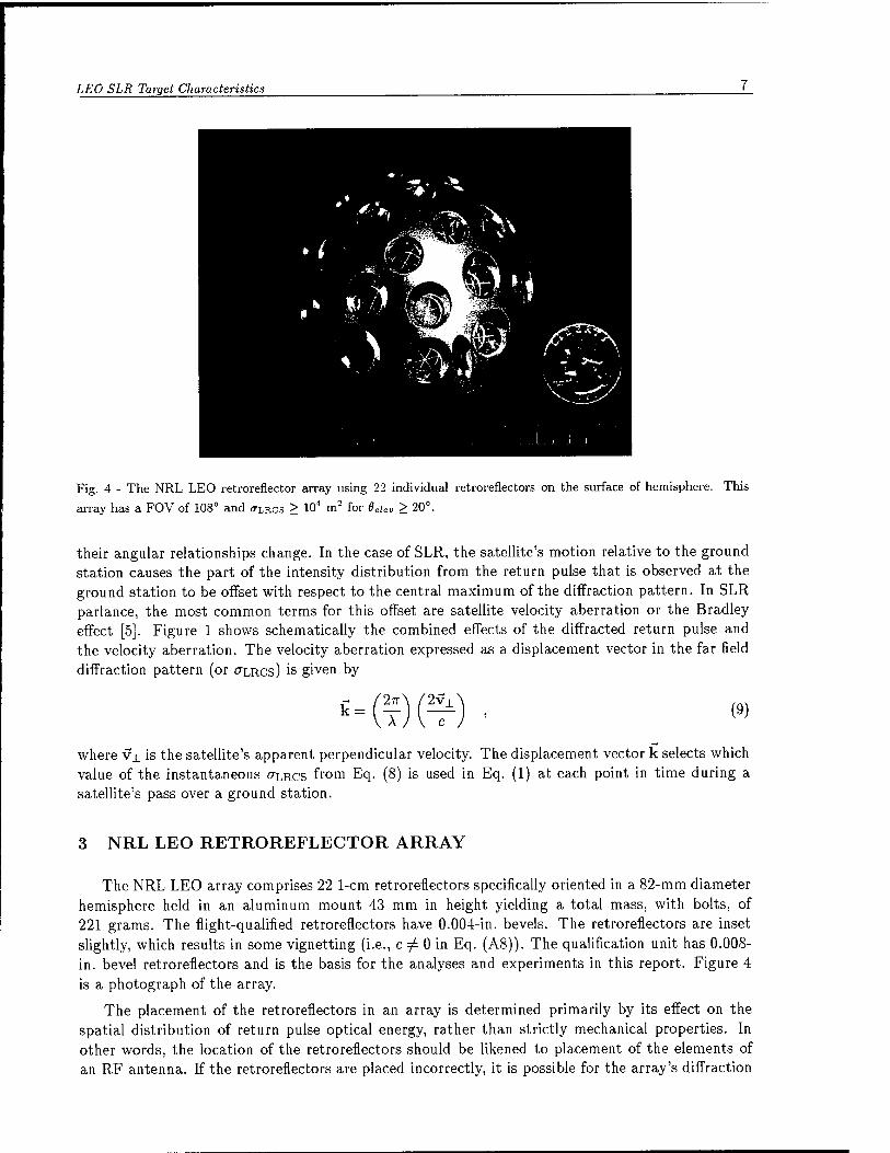
Fig. 4 - The NRL LEO retroreflector array using 22 individual retroreflectors on the surface of hemisphere. This
array has a FOV of 108° and <TLRCS > 104 m2 for 8eUv > 20°.
their angular relationships change. In the case of SLR, the satellite's motion relative to the ground station causes the part of the intensity distribution from the return pulse that is observed at the ground station to be offset with respect to the central maximum of the diffraction pattern. In SLR parlance, the most common terms for this offset are satellite velocity aberration or the Bradley effect [5]. Figure 1 shows schematically the combined effects of the diffracted return pulse and the velocity aberration. The velocity aberration expressed as a displacement vector in the far field diffraction pattern (or CTLRCS) '
S giyen by
where vj_ is the satellite's apparent perpendicular velocity. The displacement vector k selects which value of the instantaneous OLRCS from Eq. (8) is used in Eq. (1) at each point in time during a satellite's pass over a ground station.
3 NRL LEO RETROREFLECTOR ARRAY
The NRL LEO array comprises 22 1-cm retroreflectors specifically oriented in a 82-mm diameter hemisphere held in an aluminum mount 43 mm in height yielding a total mass, with bolts, of 221 grams. The flight-qualified retroreflectors have 0.004-in. bevels. The retroreflectors are inset slightly, which results in some vignetting (i.e., c ^ 0 in Eq. (A8)). The qualification unit has 0.008- in. bevel retroreflectors and is the basis for the analyses and experiments in this report. Figure 4 is a photograph of the array.
The placement of the retroreflectors in an array is determined primarily by its effect on the spatial distribution of return pulse optical energy, rather than strictly mechanical properties. In other words, the location of the retroreflectors should be likened to placement of the elements of an RF antenna. If the retroreflectors are placed incorrectly, it is possible for the array's diffraction
Gilbreath, Rolsma, Kessel, Patterson, and Georges
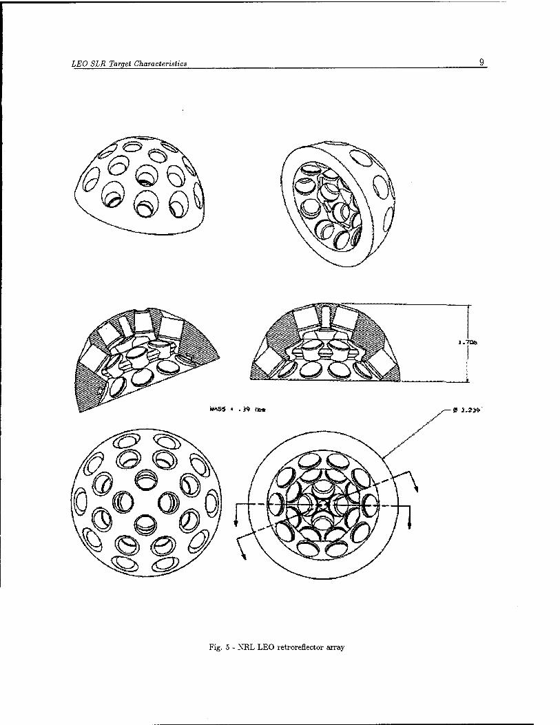
pattern to combine with the velocity aberration and generate a null at the ground station. The NRL LEO array's multiple retroreflectors are specifically placed to provide a field of view (FOV) of 108°, while neither generating such a null nor impacting timing (see Section 5.3). Figure 5 is a mechanical drawing of the array. The retroreflectors are in three rings. The first ring is at 16° with four retroreflectors placed at 0°, 90°, 180°, and 270° in azimuth. The second is at 32° with eight retroreflectors placed at 22.5°, 67.5°, 112.5°, 157.5°, 202.5°, 247.5°, 292.5°, and 337.5° in azimuth. The third is at 48° with 10 retroreflectors placed at 18°, 54°, 90°, 126°, 162°, 198°, 234°, 270°, 306°, and 342° in azimuth.
To compute predicted on-orbit SLR performance for this array, both far field diffraction ef- fects and velocity aberration must be taken into account. Our numerical approach required, as a building block, that we first develop a method to predict the on-orbit SLR performance of a single retroreflector. Consequently, we can compare the predicted performance between the NRL LEO array with that of a single retroreflector. To foreshadow Section 5.2, the returns from the array's multiple retroreflectors for a given pulse mitigates nulls of a single retroreflector OXRCS and permit a much larger FOV.
4 NUMERICAL COMPUTATION OF SATELLITE LASER RANGING PERFORMANCE
We have developed a set of numerical techniques to predict on-orbit SLR performance. The three basic problems addressed are:
1. computing the CTLRCS of a single retroreflector;
2. combining several single retroreflector CTLRCS values to determine an array's overall CTLRCS; and
3. using orbit dynamic data with the CTLRCS values to compute the actual link analysis.
This section sketches the physical basis for the numerical methods and the relative impact of different SLR properties on performance. The underlying analytic expressions and numerical im- plementation are presented in detail in Appendix A and Appendix B respectively. The experimental validation of results from these routines is discussed in Section 6.
4.1 Single Circular Retroreflector Far Field Diffraction Patterns and CTLRCS
This section discusses spatial distribution of a pulse return from a single retroreflector caused by diffraction. The section covers the results from our numerical computation of «TLRCS for four cases beginning with the highest symmetry: normal incidence without bevels; tilted incidence without bevels; normal incidence with bevels; and tilted incidence with bevels. Each case serves as a limiting test for the numerical routines of the succeeding cases.
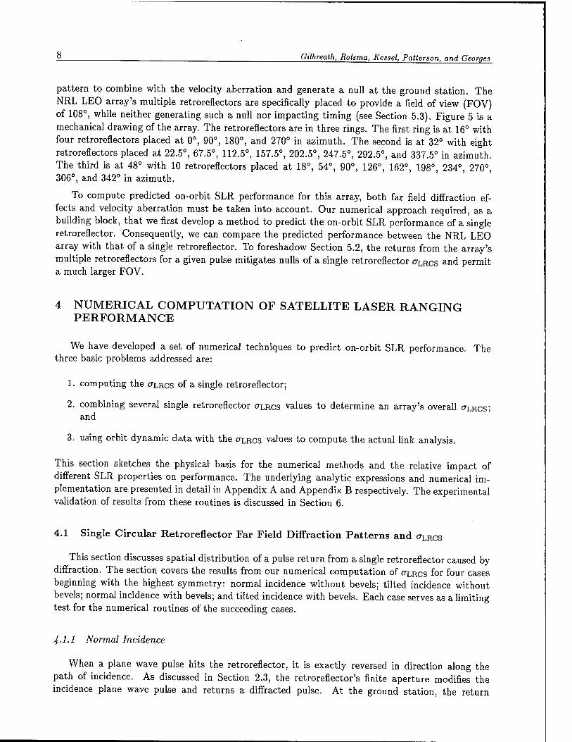
4-1-1 Normal Incidence
When a plane wave pulse hits the retroreflector, it is exactly reversed in direction along the path of incidence. As discussed in Section 2.3, the retroreflector's finite aperture modifies the incidence plane wave pulse and returns a diffracted pulse. At the ground station, the return
LEO SLR Target Characteristics
l.TOty
*—0 t.SSf'
Fig. 5 - NRL LEO retroreflector array
10 ^ Gilbreath, Rolsma, Kessel, Patterson, and Georges
pulse has the spatial distribution of the aperture's far field diffraction pattern. A single circular retroreflector without bevel losses observed at normal incidence provides a geometry with sufficiently high symmetry that an analytic expression exists for the FFDP. The FFDP is the Airy function [7, 8]; hence, from Eq. (5),
4xA2 f2J1{rk)^2
ahRCS(k) = ^{-^) , (10)
where A is the area of the retroreflector, r is the retroreflector radius, and
k = —sm0 . (11) A
At normal incidence, CTLRCS has azimuthal symmetry and Eq. (10) is a function of the single magnitude variable k only. Note that in Eq. (11), 6 is the interior angle between the +Z-axis and the observation direction in Fig. 3. It is also more convenient to plot CTLRCS in terms the equivalent 9. Even for a ö"LRCS form that lacks azimuthal symmetry, kx and ky arguments can be specified in terms of a pair of equivalent angles 6X and 6y.
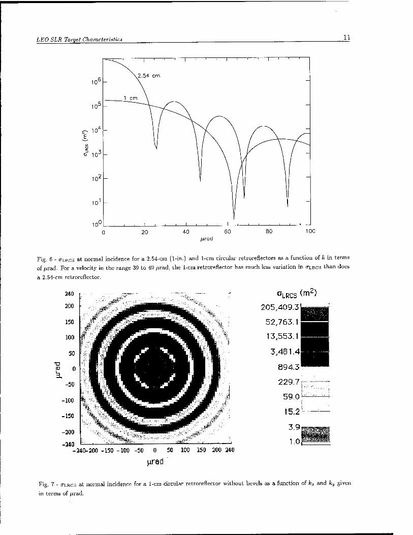
Figure 6 shows CTLRCS as function of k (a radial slice in kx, ky) for 2.54-cm and 1-cm aperture sizes. Both curves were computed numerically with the FFDP routines described in Appendix A.l and agree with Eq. (10) to machine precision. The correct geometry required for normal incidence can occur only when the satellite is directly above the ground station and the retroreflector normal is aligned with the nadir direction. The velocity aberration magnitude varies approximately over the range 39 to 49 firad for a 1,100-km circular orbit (typical LEO spacecraft) and over 38 to 48 /irad for a 1,330-km circular orbit (TOPEX/Poseidon). Thus, as can be seen in Fig. 6, although o"LRCS for the 2.54-cm retroreflector is significantly larger at k = 0, the broader FFDP of the 1-cm retroreflector can have a greater LRCS over the critical regions and certainly has greater constancy (less variation) throughout the pattern. Figure 7 is a contour plot of CTLRCS for a 1-cm circular retroreflector as a function of kx and ky in terms of /irad.
While Fig. 7 shows CTLRCS over a sizable angular region of the far field, the observation of return pulse is made at a single kx, ky point. The velocity aberration given by Eq. (9) selects this single kx, ky point and, consequently, the OXRCS value used in Eq. (1) during the link margin computation. To provide a scale length, for an 1,100-km orbit, the corner points of Fig. 7 at ±240 /xradians correspond to ±0.264-km distances.
4-1-2 Off-axis Incidence
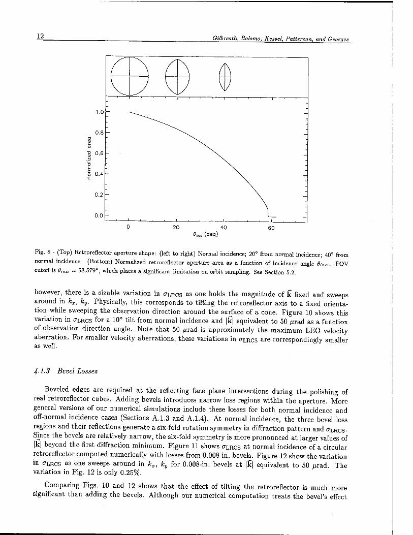
At all other points in an orbital pass, the retroreflector tips away from normal incidence, so its projected aperture changes in shape and decreases in area. Figure 8 shows how both the shape of the projected aperture and the area changes as a function of incidence angle 0,-nct-. Note that the projected aperture decreases in size along both axes. The decrease in projected aperture size increases the angular extent of the FFDP proportionally and decreases its overall magnitude. The change in aperture shape eliminates azimuthal symmetry so an analytic closed-form expression for the FFDP (e.g., Airy function) is no longer possible. Appendix A.l describes a method to numerically compute the FFDP.
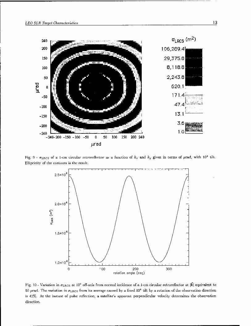
Figure 9 shows CTLRCS of a tilted 1-cm circular retroreflector computed numerically without bevel losses. The azimuthal symmetry present for normal incidence has been reduced to a two-fold rotational symmetry as seen from the ellipticity of the contours. The central maximum around kx — ky = 0 remains smoothly rounded. For observations made away from the central maximum,
LEO SLR Target Characteristics 11
100 /j.rad
Fig. 6 - (TLRC3 at normal incidence for a 2.54-cm (1-in.) and 1-crn circular retroreflectors as a function of k in terms
of /jrad. For a velocity in the range 39 to 49 ^rad, the 1-cm retroreflector has much less variation in CTLRCS than does
a 2.54-cm retroreflector.
59.0f-
15.2 —
3-9f;;.^liV-J
1.0 -240- 200 -150 -100 -50 50 100 150 200 240
^rad
Fig. 7 - (TLRC5 at normal incidence for a 1-cm circular retroreflector without bevels as a function of kx and ky given
in terms of ^rad.
12 Gilbreath, Rolsma, Kessel, Patterson, and Georges
1.0
0.8
0.6
0.4
0.2
0.0
20 40 0i„c; (deg)
60
Fig. 8 - (Top) Retroreflector aperture shape: (left to right) Normal incidence; 20° from normal incidence; 40° from
normal incidence. (Bottom) Normalized retroreflector aperture area as a function of incidence angle 0;nci. FOV
cutoff is Oinci = 58.579°, which places a significant limitation on orbit sampling. See Section 5.2.
however, there is a sizable variation in CTLRCS as one holds the magnitude of k fixed and sweeps around in kx, ky. Physically, this corresponds to tilting the retroreflector axis to a fixed orienta- tion while sweeping the observation direction around the surface of a cone. Figure 10 shows this variation in CTLRCS
for a 10° tilt from normal incidence and |k| equivalent to 50 yurad as a function of observation direction angle. Note that 50 /zrad is approximately the maximum LEO velocity aberration. For smaller velocity aberrations, these variations in CTLRCS
are correspondingly smaller as well.
4-1-3 Bevel Losses
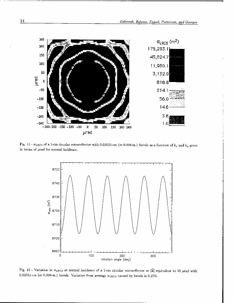
Beveled edges are required at the reflecting face plane intersections during the polishing of real retroreflector cubes. Adding bevels introduces narrow loss regions within the aperture. More general versions of our numerical simulations include these losses for both normal incidence and off-normal incidence cases (Sections A. 1.3 and A. 1.4). At normal incidence, the three bevel loss regions and their reflections generate a six-fold rotation symmetry in diffraction pattern and ahRCS. Since the bevels are relatively narrow, the six-fold symmetry is more pronounced at larger values of |k| beyond the first diffraction minimum. Figure 11 shows O"LRCS at normal incidence of a circular retroreflector computed numerically with losses from 0.008-in. bevels. Figure 12 show the variation in CTLRCS as one sweeps around in kx, ky for 0.008-in. bevels at |k| equivalent to 50 /irad. The variation in Fig. 12 is only 0.25%.
Comparing Figs. 10 and 12 shows that the effect of tilting the retroreflector is much more significant than adding the bevels. Although our numerical computation treats the bevel's effect
LEO SLR Target Characteristics 13
-240-200 -150 -100 -50 0 50 100 150 200 240
Fig. 9 - (TLEC5 of a 1-cm circular retroreflector as a function of kx and ky given in terms of /irad, with 10° tilt.
Ellipticity of the contours is the result.
2.5X1CT -
2.0xlCT
1.5X1CT
1.0x10 -
_j ! 1 ! j ! , p—p-
100 200 rotation angle (deg)
300
Fig. 10 - Variation in <TLRCS at 10° off-axis from normal incidence of a 1-cm circular retroreflector at |k| equivalent to
50 £jrad. The variation in OXRCS from its average caused by a fixed 10° tilt by a rotation of the observation direction
is 42%. At the instant of pulse reflection, a satellite's apparent perpendicular velocity determines the observation
direction.
14 Gilbreath, Rolsma, Kessel, Patterson, and Georges
-240-200 -150 -100 -50 0 50 100 150 200 240
Fig. 11 - (TLRCS of a 1-cm circular retroreflector with 0.02032-cm (or 0.008-in.) bevels as a function of kx and ky given in terms of jjrad for normal incidence.
8750
8690 h
100 200 rotation angle (deg)
300
Fig. 12 - Variation in £rLRC3 at normal incidence of a 1-cm circular retroreflector at |k| equivalent to 50 ^irad with
0.02032-cm (or 0.008-in.) bevels. Variation from average <TLRC3 caused by bevels is 0.25%
LEO SLR Target Characteristics 15
exactly, to first order, the bevels could also be considered as simply a scalar loss of reflecting area combined with a slightly reduced FOV. The combination of both retroreflector tilt and bevel losses requires a slightly more complex numerical simulation, but it does not introduce any qualitatively new features to the FFDP or outcs-
4.2 Retroreflector Array Far Field Diffraction Patterns and CTLRCS
The return pulse is the sum of the contributions from several retroreflectors in the array. The total FFDP ä for the array of L retroreflectors at a given instant of time is
ä = £äie*'a« (12) /=i
where the a/s are the phase angles for each retroreflector for a given incidence direction. From Eq. (8), the instantaneous LRCS is
Ait CTLRCS =pp-|öä*|
Upon substitution:
^LRCS AlT
4TT
(I! ame,"or-) (S fi^«"fa") L L
£ 2 ämäne x* J(am-an)
m=\ n=l
(13)
(14)
(15)
During a brief interval r, variations of phase angle relationships between individual retroreflec- tors can occur. Provided the statistical correlation between am and an over r is small, one is free to treat resulting phase factors as essentially random fluctuations. Consequently, a time-averaged LRCS will simplify to:
^LRCS 47T
Air
L L - y^ V^ "m". [r ei[a{t)m-a(t)n]dt
7i=l n=l
= PT2YI I5« A2
(16)
(17) m=l
For SLR measurements with precisions significantly tighter than ±1 cm, r may be become small enough that the phase integral cannot be considered as a Kronecker delta function Smn. For the LEO application, however, using a random phase approximation is sufficient, and the array's LRCS can be evaluated using the incoherent sum of the contributions in Eq. (17).
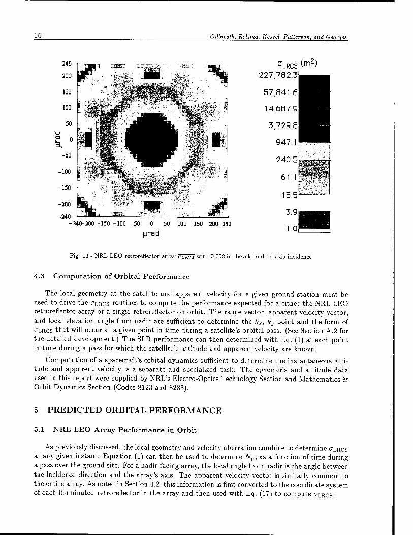
Equation (17) is a convenient form for numerical evaluation. The routines developed and tested in the single retroreflector can be used directly to compute the ams. The primary addition is a routine that combines an incidence direction with respect to the array's axis with individual retroreflector directions to determine which retroreflectors are illuminated within their FOV limits and at what angles. It is then straightforward to compute the relevant äms and to sum to obtain ÖLRCS- Figure 13 shows CTLRCS of the array (using retroreflectors with 0.008-in. bevels) as computed numerically when viewed along the array's axis. (Note that array CTLRCS
vames used in Section 5 are time-averaged. Unless there is a specific reason to do otherwise, explicit notation of the time- averaging is suppressed for the balance of this report.)
16 Gilbreath, Rolsma, Kessel, Patterson, and Georges
cLRC3 (m2)
227,782.31
-240-200 -150 -100 -50 0 50 100 150 200 240
pirad
Fig. 13 - NRL LEO retroreflector array <TLRCS with 0.008-in. bevels and on-axis incidence
4.3 Computation of Orbital Performance
The local geometry at the satellite and apparent velocity for a given ground station must be used to drive the CTLRCS routines to compute the performance expected for a either the NRL LEO retroreflector array or a single retroreflector on orbit. The range vector, apparent velocity vector, and local elevation angle from nadir are sufficient to determine the kx, ky point and the form of CLRCS that will occur at a given point in time during a satellite's orbital pass. (See Section A.2 for the detailed development.) The SLR performance can then determined with Eq. (1) at each point in time during a pass for which the satellite's attitude and apparent velocity are known.
Computation of a spacecraft's orbital dynamics sufficient to determine the instantaneous atti- tude and apparent velocity is a separate and specialized task. The ephemeris and attitude data used in this report were supplied by NRL's Electro-Optics Technology Section and Mathematics & Orbit Dynamics Section (Codes 8123 and 8233).
5 PREDICTED ORBITAL PERFORMANCE
5.1 NRL LEO Array Performance in Orbit
As previously discussed, the local geometry and velocity aberration combine to determine O^RCS
at any given instant. Equation (1) can then be used to determine Npe as a function of time during a pass over the ground site. For a nadir-facing array, the local angle from nadir is the angle between the incidence direction and the array's axis. The apparent velocity vector is similarly common to the entire array. As noted in Section 4.2, this information is first converted to the coordinate system of each illuminated retroreflector in the array and then used with Eq. (17) to compute CTLRCS-
LEO SLR Target Characteristics 17
1.5x10-
E 1.0x10"
5.0x10^
22-element array
5.52x10 5.54x10 5.56x10^ Time (s)
5.58x10^
Fig. 14 - (TLRcs of the 22-element NRL LEO retroreflector array at 532 and 1064 nm (top) and 6etev (bottom) as a
function of time; this is a near-zenith pass over MRC with 9eiev = 88° at PCA
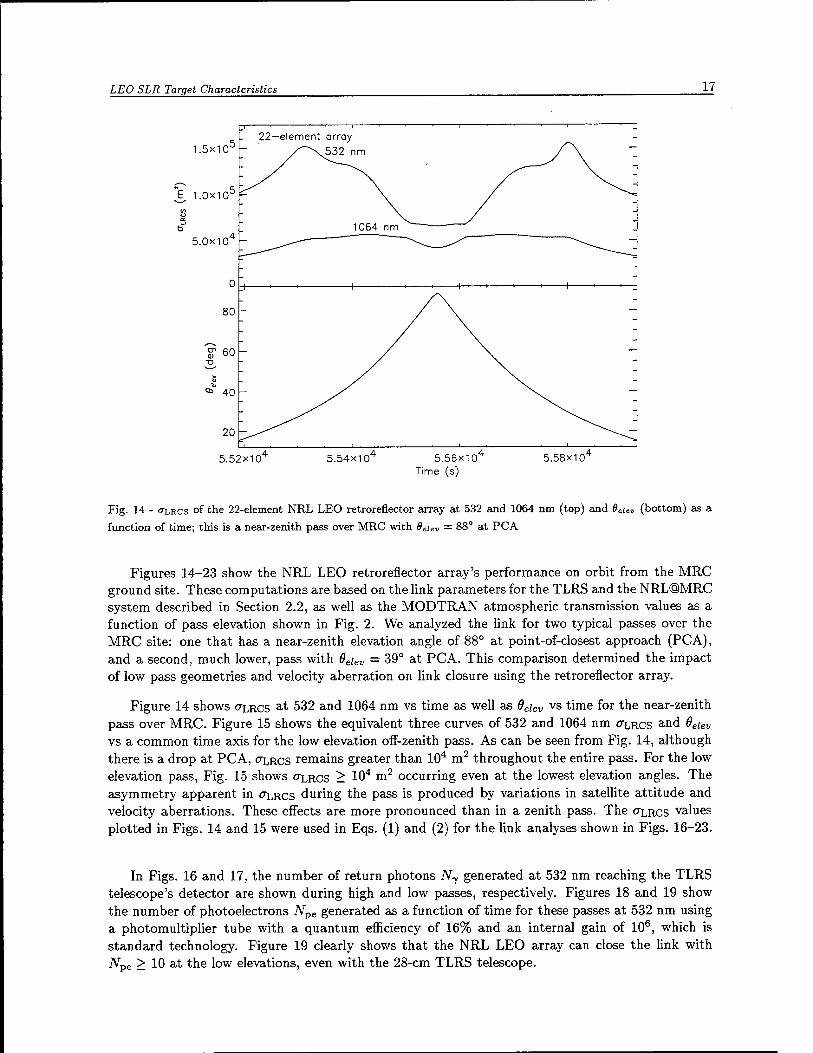
Figures 14-23 show the NRL LEO retroreflector array's performance on orbit from the MRC ground site. These computations are based on the link parameters for the TLRS and the NRL@MRC system described in Section 2.2, as well as the MODTRAN atmospheric transmission values as a function of pass elevation shown in Fig. 2. We analyzed the link for two typical passes over the MRC site: one that has a near-zenith elevation angle of 88° at point-of-closest approach (PCA), and a second, much lower, pass with 6eiev = 39° at PCA. This comparison determined the impact of low pass geometries and velocity aberration on link closure using the retroreflector array.
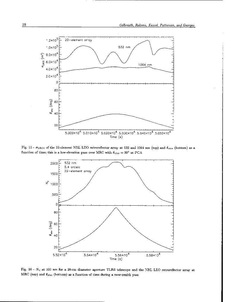
Figure 14 shows CTLRCS at 532 and 1064 nm vs time as well as 6eiev vs time for the near-zenith
pass over MRC. Figure 15 shows the equivalent three curves of 532 and 1064 nm (TLRCS and 6eiev
vs a common time axis for the low elevation off-zenith pass. As can be seen from Fig. 14, although there is a drop at PCA, ULRCS remains greater than 104 m2 throughout the entire pass. For the low elevation pass, Fig. 15 shows <TLRCS > 104 m2 occurring even at the lowest elevation angles. The asymmetry apparent in CTLRCS during the pass is produced by variations in satellite attitude and velocity aberrations. These effects are more pronounced than in a zenith pass. The CLRCS values plotted in Figs. 14 and 15 were used in Eqs. (1) and (2) for the link analyses shown in Figs. 16-23.
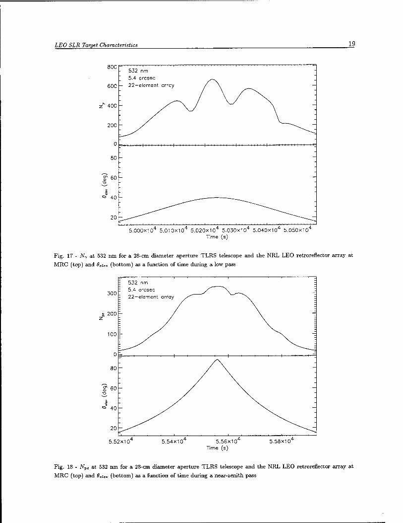
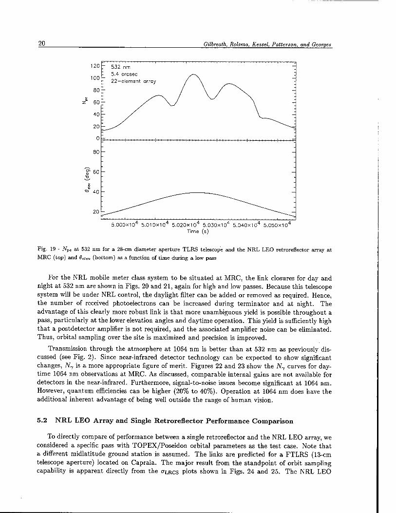
In Figs. 16 and 17, the number of return photons N^ generated at 532 nm reaching the TLRS telescope's detector are shown during high and low passes, respectively. Figures 18 and 19 show the number of photoelectrons Npe generated as a function of time for these passes at 532 nm using a photomultiplier tube with a quantum efficiency of 16% and an internal gain of 106, which is standard technology. Figure 19 clearly shows that the NRL LEO array can close the link with iVpe > 10 at the low elevations, even with the 28-cm TLRS telescope.
18 Gilbreath, Rolsma, Kessel, Patterson, and Georges
1.2x10'
2.0x10
0
80
60
i ■ i i I I 'I t I t I * I I 'I ) I ' t» t - 4--4- 4
5.000x10⁴ 5.010x10⁴ 5.020x10⁴ 5.030X10⁴ 5.040X10⁴ 5.050x10⁴
Time (s)
Fig. 15 - «TLRCS of the 22-element NRL LEO retroreflector array at 532 and 1064 nm (top) and 8euv (bottom) as a
function of time; this is a low-elevation pass over MRC with 0eiev = 39° at PCA
2000
1500
1000
532 nm 5.4 arcsec 22—element array
5.52x10' 5.54x10 5.56x10^ Time (s)
5.58x10^
Fig. 16 - N-, at 532 nm for a 28-cm diameter aperture TLRS telescope and the NRL LEO retroreflector array at
MRC (top) and 0eiet, (bottom) as a function of time during a near-zenith pass
LEO SLR Target Characteristics 19
800
600
400
200 -
532 nm 5.4 arcsec
— 22-element array
0
80
60
I I ' I'''
5.000X10⁴ 5.010X10⁴ 5.020x10⁴ 5.030x10⁴ 5.040X10⁴ 5.050x10⁴
Time (s)
Fig. 17 - N-, at 532 nm for a 28-cm diameter aperture TLRS telescope and the NRL LEO retroreflector array at
MRC (top) and 6eiev (bottom) as a function of time during a low pass
: 532 nm : 5.4 arcsec
22-element array
g. 200 '-
100 E-
5.52x10' 5.54x10' 5.56x10^ Time (s)
5.58x10^
Fig. 18 - iVpe at 532 nm for a 28-cm diameter aperture TLRS telescope and the NRL LEO retroreflector array at
MRC (top) and 9euv (bottom) as a function of time during a near-zenith pass
20 Gilbreath, Rolsma, Kessel, Patterson, and Georges
120
100
80
z 60
40
20
0
80
1? 60
532 nm 5.4 orcsec 22-element array
■**+- I |II I
5.000X10⁴ 5.010x10⁴ 5.020X10⁴ 5.030X10⁴ 5.040X10⁴ 5.050X10⁴
Time (s)
Fig. 19 - Npe at 532 nm for a 28-cm diameter aperture TLRS telescope and the NRL LEO retroreflector array at
MRC (top) and 6euv (bottom) as a function of time during a low pass
For the NRL mobile meter class system to be situated at MRC, the link closures for day and night at 532 nm are shown in Figs. 20 and 21, again for high and low passes. Because this telescope system will be under NRL control, the daylight filter can be added or removed as required. Hence, the number of received photoelectrons can be increased during terminator and at night. The advantage of this clearly more robust link is that more unambiguous yield is possible throughout a pass, particularly at the lower elevation angles and daytime operation. This yield is sufficiently high that a postdetector amplifier is not required, and the associated amplifier noise can be eliminated. Thus, orbital sampling over the site is maximized and precision is improved.
Transmission through the atmosphere at 1064 nm is better than at 532 nm as previously dis- cussed (see Fig. 2). Since near-infrared detector technology can be expected to show significant changes, iV7 is a more appropriate figure of merit. Figures 22 and 23 show the iV7 curves for day- time 1064 nm observations at MRC. As discussed, comparable internal gains are not available for detectors in the near-infrared. Furthermore, signal-to-noise issues become significant at 1064 nm. However, quantum efficiencies can be higher (20% to 40%). Operation at 1064 nm does have the additional inherent advantage of being well outside the range of human vision.
5.2 NRL LEO Array and Single Retroreflector Performance Comparison
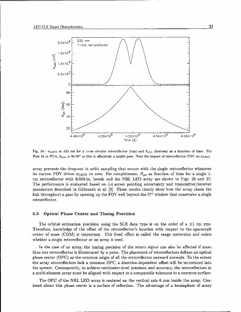
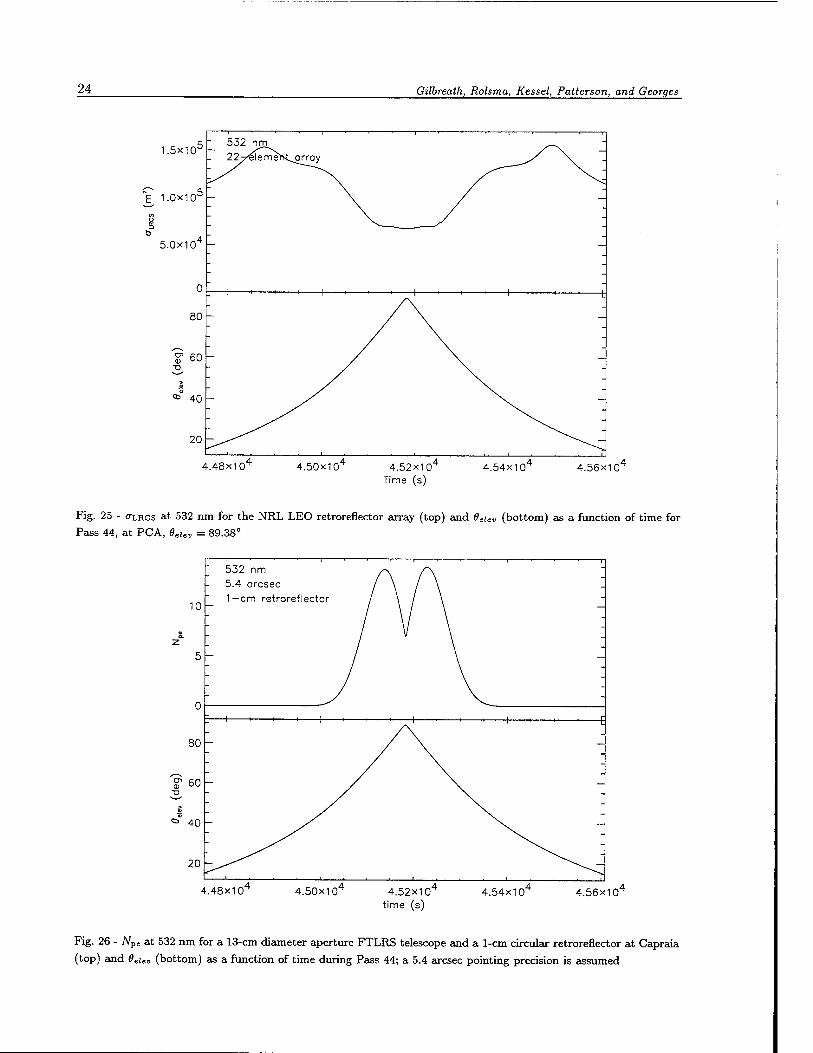
To directly compare of performance between a single retroreflector and the NRL LEO array, we considered a specific pass with TOPEX/Poseidon orbital parameters as the test case. Note that a different midlatitude ground station is assumed. The links are predicted for a FTLRS (13-cm telescope aperture) located on Capraia. The major result from the standpoint of orbit sampling capability is apparent directly from the CTLRCS plots shown in Figs. 24 and 25. The NRL LEO
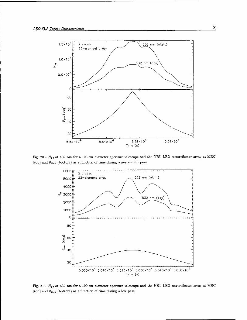
LEO SLR Target Characteristics 21
1.5x10
1.0x10 -
5.0x10
5.52x10 5.54x10 5.56x10^ Time (s)
5.58x10^
Fig. 20 - Npc at 532 nm for a 100-cm diameter aperture telescope and the NRL LEO retroreflector array at MRC
(top) and QeUv (bottom) as a function of time during a near-zenith pass
6000
5000
4000
1 3000
2000
1000
0
80
If 60 >
«a* 40
20 -
2 arcsec 22-element array 532 nm (night)
5.000X10⁴ 5.010X10⁴ 5.020X10⁴ 5.030X10⁴ 5.040X10⁴ 5.050x10⁴
Time (s)
Fig. 21 - iVpe at 532 nm for a 100-cm diameter aperture telescope and the NRL LEO retroreflector array at MRC
(top) and öeieu (bottom) as a function of time during a low pass
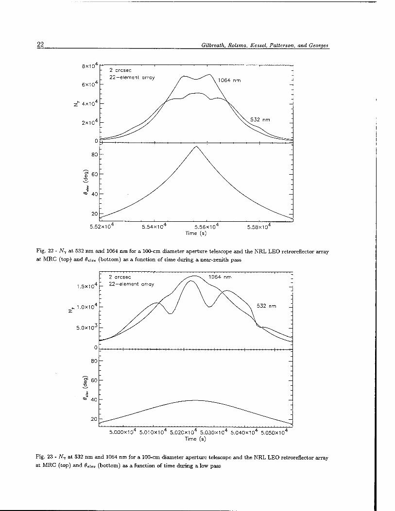
22 Gilbreath, Rolsma, Kessel, Patterson, and Georges
8X1CT
6x10
4x10
2x10
2 arcsec 22—element array 1064 nm
5.52x10 5.54x10 5.56x10^ Time (s)
5.58x10^
Fig. 22 - Nf at 532 nm and 1064 nm for a 100-cm diameter aperture telescope and the NRL LEO retroreflector array
at MRC (top) and 6eUv (bottom) as a function of time during a near-zenith pass
.5x10^
*. 1.0X1CT
5.0x10-
0
80
60
2 arcsec 1. 22-element array
' | i i ' i i i i i i | i t i i i i i i i | i i i i i i i i i i i i i i i i i i i | i i i i i i i i i
S.OOOxlO4 5.010X10⁴ 5.020X10⁴ 5.030x10⁴ 5.040x10⁴ 5.050x10⁴
Time (s)
Fig. 23 - iV-y at 532 nm and 1064 nm for a 100-cm diameter aperture telescope and the NRL LEO retroreflector array
at MRC (top) and 6eiev (bottom) as a function of time during a low pass
LEO SLR Target Characteristics 23
2.0X1CT
^ 1.5x10⁴
o 1.0x10' to
5.0x10'
532 nm 1 -cm retroreflector
4.48x10 4.50x10 4.52x10 Time (s)
4.54x10 4.56x10
Fig. 24 - CTLRCS at 532 nm for a 1-cm circular retroreflector (top) and 8eiev (bottom) as a function of time. For
Pass 44 at PCA, öe;e„ = 89.38° so this is effectively a zenith pass. Note the impact of retroreflector FOV on OXRCS
array prevents the drop-out in orbit sampling that occurs with the single retroreflector whenever its narrow FOV drives CTLRCS *° zero. For completeness, Npe as function of time for a single 1- cm retroreflector with 0.008-in. bevels and the NRL LEO array are shown in Figs. 26 and 27. The performance is evaluated based on 5.4 arcsec pointing uncertainty and transmitter/receiver parameters described in Gilbreath et al. [9]. These results clearly show how the array closes the link throughout a pass by opening up the FOV well beyond the 57° window that constrains a single retroreflector.
5.3 Optical Phase Center and Timing Precision
The orbital estimation precision using the SLR data type is on the order of a ±1 cm rms. Therefore, knowledge of the offset of the retroreflector's location with respect to the spacecraft center of mass (COM) is important. This fixed offset is called the range correction and exists whether a single retroreflector or an array is used.
In the case of an array, the timing precision of the return signal can also be affected if more than one retroreflector is illuminated by a pulse. The placement of retroreflectors defines an optical phase center (OPC) as the common origin of all the retroreflector outward normals. To the extent the array retroreflectors lack a common OPC, a direction-dependent offset will be introduced into the system. Consequently, to achieve centimeter-level precision and accuracy, the retroreflectors in a multi-element array must be aligned with respect to a comparable tolerance to a common surface.
The OPC of the NRL LEO array is centered on the vertical axis 6 mm inside the array. Cen- tered about this phase center is a surface of reflection. The advantage of a hemisphere of many
24 Gilbreath, Rolsma, Kessel, Patterson, and Georges
1.5X1CT
£ 1.0x10"
5.0x10
4.48x10 4.50x10' 4.52x10^ Time (s)
4.54x10^ 4.56x10M
Fig. 25 - OXRCS at 532 nm for the NRL LEO retroreflector array (top) and 9eicv (bottom) as a function of time for Pass 44, at PCA, 6eUv = 89.38°
532 nm 5.4 arcsec 1 —cm retroreflector
4.48x10 4.50x10 4.52x10^ time (s)
4.54x10^ 4.56x10^
Fig. 26 - ATpe at 532 nm for a 13-cm diameter aperture FTLRS telescope and a 1-cm circular retroreflector at Capraia
(top) and 9euv (bottom) as a function of time during Pass 44; a 5.4 arcsec pointing precision is assumed
LEO SLR Target Characteristics 25
532 nm 5.4 arcsec 22-element array
4.48x10' 4.50x10 4.52x10^ Time (s)
4.54x10 4.56x10
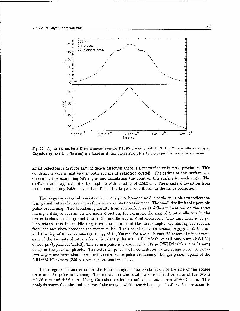
Fig. 27 - Afp«, at 532 nm for a 13-cm diameter aperture FTLRS telescope and the NRL LEO retroreflector array at
Capraia (top) and 6eiev (bottom) as a function of time during Pass 44; a 5.4 arcsec pointing precision is assumed
small reflectors is that for any incidence direction there is a retroreflector in close proximity. This condition allows a relatively smooth surface of reflection overall. The radius of this surface was determined by examining 585 angles and calculating the point on this surface for each angle. The surface can be approximated by a sphere with a radius of 2.505 cm. The standard deviation from this sphere is only 0.086 cm. This radius is the largest contributor to the range correction.
The range correction also must consider any pulse broadening due to the multiple retroreflectors. Using small retroreflectors allows for a very compact arrangement. The small size limits the possible pulse broadening. The broadening results from retroreflectors at different locations on the array having a delayed return. In the nadir direction, for example, the ring of 4 retroreflectors in the center is closer to the ground than is the middle ring of 8 retroreflectors. The time delay is 66 ps. The return from the middle ring is smaller because of the larger angle. Combining the returns from the two rings broadens the return pulse. The ring of 4 has an average CTLRCS of 52,000 m2
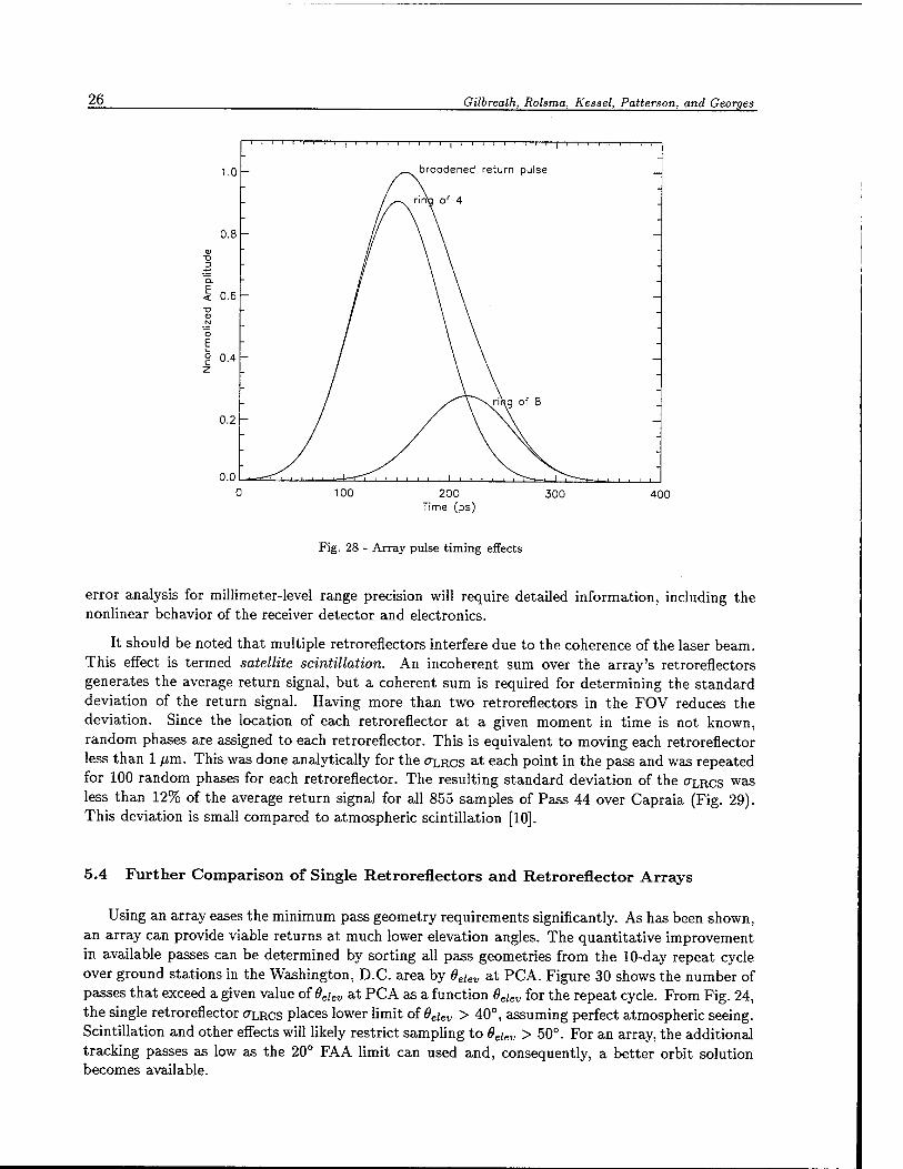
and the ring of 8 has an average CTLRCS of 16,000 m2, for nadir. Figure 28 shows the incoherent sum of the two sets of returns for an incident pulse with a full width at half maximum (FWHM) of 100 ps (typical for TLRS). The return pulse is broadened to 117 ps FWHM with a 7 ps (1 mm) delay in the peak amplitude. The extra 17 ps of width contributes to the range error. A 1-mm two way range correction is required to correct for pulse broadening. Longer pulses typical of the NRL@MRC system (250 ps) would have smaller effects.
The range correction error for the time of flight is the combination of the size of the sphere error and the pulse broadening. The increase in the total standard deviation error of the two is ±0.86 mm and ±2.6 mm. Using Gaussian statistics results in a total error of ±2.74 mm. This analysis shows that the timing error of the array is within the ±1 cm specification. A more accurate
26 Gilbreatk, Rolsma, Kessel, Patterson, and Georges
_ ' 1 | i l ■ l l l l l l | i i i —i—i—i—i—]—
1.0 - ^_^ broadened return pulse -
- /s^\ ring of 4 -
0.8 - _
Am
plit
ud
e
o
en
-
"O
N ; -
§ ° 0.4 - :
- - i _
/T\ri)w of 8 _ 0.2 —
0.0 .a—r—it I I I i ̂ ■—1—r i _i—i—i—i_..i__i i 1 i t T i i ii i—i_. 1 i i—,—i
100 200 Time (ps)
300 400
Fig. 28 - Array pulse timing effects
error analysis for millimeter-level range precision will require detailed information, including the nonlinear behavior of the receiver detector and electronics.
It should be noted that multiple retroreflectors interfere due to the coherence of the laser beam. This effect is termed satellite scintillation. An incoherent sum over the array's retroreflectors generates the average return signal, but a coherent sum is required for determining the standard deviation of the return signal. Having more than two retroreflectors in the FOV reduces the deviation. Since the location of each retroreflector at a given moment in time is not known, random phases are assigned to each retroreflector. This is equivalent to moving each retroreflector less than 1 /im. This was done analytically for the OXR.CS
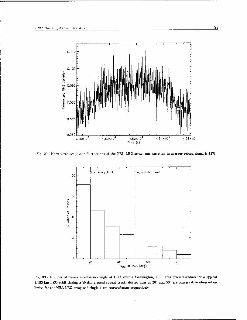
at eac'1 Point in the pass and was repeated for 100 random phases for each retroreflector. The resulting standard deviation of the CTLRCS was less than 12% of the average return signal for all 855 samples of Pass 44 over Capraia (Fig. 29). This deviation is small compared to atmospheric scintillation [10].
5.4 Further Comparison of Single Retroreflectors and Retroreflector Arrays
Using an array eases the minimum pass geometry requirements significantly. As has been shown, an array can provide viable returns at much lower elevation angles. The quantitative improvement in available passes can be determined by sorting all pass geometries from the 10-day repeat cycle over ground stations in the Washington, D.C. area by 0eiev at PCA. Figure 30 shows the number of passes that exceed a given value of 6eiev at PCA as a function 6eiev for the repeat cycle. From Fig. 24, the single retroreflector CTLRCS places lower limit oiOeiev > 40°, assuming perfect atmospheric seeing. Scintillation and other effects will likely restrict sampling to 9eiev > 50°. For an array, the additional tracking passes as low as the 20° FA A limit can used and, consequently, a better orbit solution becomes available.
LEO SLR Target Characteristics 27
0.110
0.060
4.48x10 4.50x10' 4.52x10^ Time (s)
4.54x10^ 4.56x10
Fig. 29 - Normalized amplitude fluctuations of the NRL LEO array; rms variation in average return signal is 12%
1 , . i | i 1 1 ' ' ' 1 '
LEO Array limit Single Retro limit 80
—
-
- 60 -
en <D tn en o 0.
-
o
o 40 - E 2
-
<
- 20 -
"
'
" _
0 , 20 40 60
6elev ot PCA (deg) 80
Fig. 30 - Number of passes vs elevation angle at PCA over a Washington, D.C. area ground station for a typical
1,100-km LEO orbit during a 10-day ground repeat track; dotted lines at 20° and 50° are conservative observation
limits for the NRL LEO array and single 1-cm retroreflector respectively
28 Gilbreath, Rolsma, Kessel, Patterson, and Georges
Spectra Physics Argon-ion
Periscope Assembly r \
Pixel 211 CCD Baffle i
Beam Expander/) Collimator
fl* =400mm f2= =3.0m f3= =120mm* f4* *300mm* *Achromatic
D1 ->2 « f 1 + f2 D2 ->3 = f 2 + f 3 D3->4 = f3 + f4 D4->CCD = f4
Array
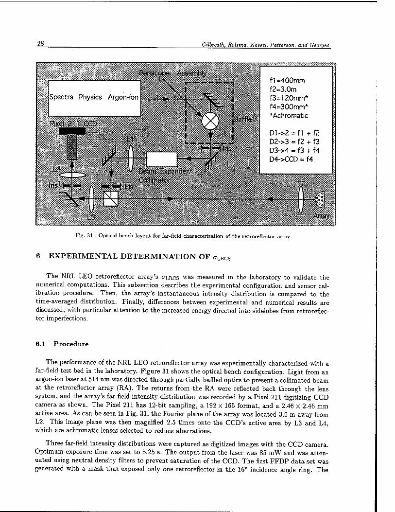
Fig. 31 - Optical bench layout for far-field characterization of the retroreflector array
6 EXPERIMENTAL DETERMINATION OF <7LRCs
The NRL LEO retroreflector array's CTLRCS was measured in the laboratory to validate the
numerical computations. This subsection describes the experimental configuration and sensor cal- ibration procedure. Then, the array's instantaneous intensity distribution is compared to the time-averaged distribution. Finally, differences between experimental and numerical results are discussed, with particular attention to the increased energy directed into sidelobes from retroreflec- tor imperfections.
6.1 Procedure
The performance of the NRL LEO retroreflector array was experimentally characterized with a far-field test bed in the laboratory. Figure 31 shows the optical bench configuration. Light from an argon-ion laser at 514 nm was directed through partially baffled optics to present a collimated beam at the retroreflector array (RA). The returns from the RA were reflected back through the lens system, and the array's far-field intensity distribution was recorded by a Pixel 211 digitizing CCD camera as shown. The Pixel 211 has 12-bit sampling, a 192 x 165 format, and a 2.46 x 2.46 mm active area. As can be seen in Fig. 31, the Fourier plane of the array was located 3.0 m away from L2. This image plane was then magnified 2.5 times onto the CCD's active area by L3 and L4, which are achromatic lenses selected to reduce aberrations.
Three far-field intensity distributions were captured as digitized images with the CCD camera. Optimum exposure time was set to 5.25 s. The output from the laser was 85 mW and was atten- uated using neutral density filters to prevent saturation of the CCD. The first FFDP data set was generated with a mask that exposed only one retroreflector in the 16° incidence angle ring. The
LEO SLR Target Characteristics 29
second and third data sets were obtained for the full RA instantaneous FFDP and time-averaged FFDP respectively.
6.2 Calibration
The CCD camera provided a digitized image of the FFDP. However, to relate the distribution from raw pixel values to angular position in //rad and CTLRCS in m2, the sensor has to be calibrated and conversion constants generated.
6.2.1 Spatial Calibration
For the spatial calibration, the optical layout shown in Fig. 31 was used with the retroreflector array replaced by a circular aperture followed by a flat mirror. A circular aperture/flat mirror combination observed at normal incidence has the same high symmetry geometry as a normal incidence single retroreflector, and the FFDP follows the Airy function form [Eq. (10)]. The known angular dependence of an Airy function served as the basis of the spatial calibration. With the mirror's normal aligned to the L2/L3 optical axis, an Airy pattern was projected onto the CCD. Images of the projected Airy pattern were recorded with the CCD for 12 apertures with radius from 7 to 18 mm in 1-mm steps. The weighted x2 difference between the observed intensity distribution on the CCD and an Airy intensity distribution, Eq. (10), was then determined as a function of the scaling parameter £ along a radial slice across the image. The scaling parameter £ converts the CCD pixel number to an angle. The minimum weighted \2 value then determines the best fit Airy pattern for a given aperture, and consequently, relates a pixel's number on the CCD a;,- to angular position from
2TT £xi = r— sin0 . (18)
A
Based on this procedure, the resulting spatial scaling coefficient S is 0.156 fir&d/fim, with a 5.6% standard deviation. 5 also has a detectable systematic variation with aperture size believed to be due the optical system's point spread function, which was measured to be ~ 70 /xm in width.
6.2.2 Radiometrie Intensity Calibration
The CCD camera flat field correction and intensity calibration were determined by imaging an integrating sphere at several power levels. Light from the 514-nm laser was directed into an integrating sphere. A UDT S370 Optometer measured the power exiting a perpendicular port. The UDT was then replaced with the CCD camera, and an image was recorded. To assure stability of laser output, a second UDT monitored secondary scatter from one of the mirrors in the optical train leading to the integrating sphere. Initially, the laser light intensity was set so that the pixels in the CCD camera all read close to their maximum value but were not saturated. The light was then attenuated in steps to the UDT's detection range limit. Images and UDT readings of the sphere were recorded for 23 different attenuations.
For each of the CCD camera's 31,680 pixels, a linear least-squares fit yielded
Pixel Value(i, j) = g [id(i, j) + R(i, j) (UDT Reading)] , (19) -
30 Gilbreath, Rolsma, Kessel, Patterson, and Georges
0 50 100 150 200 250 300 374
LRCS
57770.3
51351.4
44932.4
38513.5
32094.6
25675.7
19256.8
12837.8
6418.92
Israel
Fig. 32 - Experimental £rLRCs for a single retroreflector at a 16° tilt from normal
where g is the analog to digital gain and id{i,j) and TZ(i,j) are the dark current and responsivity of the i,j pixel, respectively. Equation (19) can be inverted to convert the raw 12-bit data into images with units of W/cm2.
The relation CTLRCS = p"^2 holds on the optical axis. This determines the coefficient C that scales the calibrated CCD output in W/cm2 to auics in m2- The coefficient C has a mean value of 0.00056, with a standard deviation of 22% for six different aperture diameters.
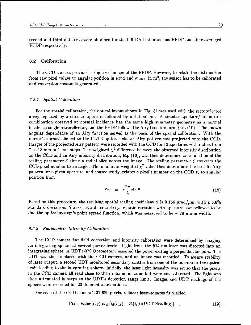
6.3 Results and Comparison to Numerical Computation
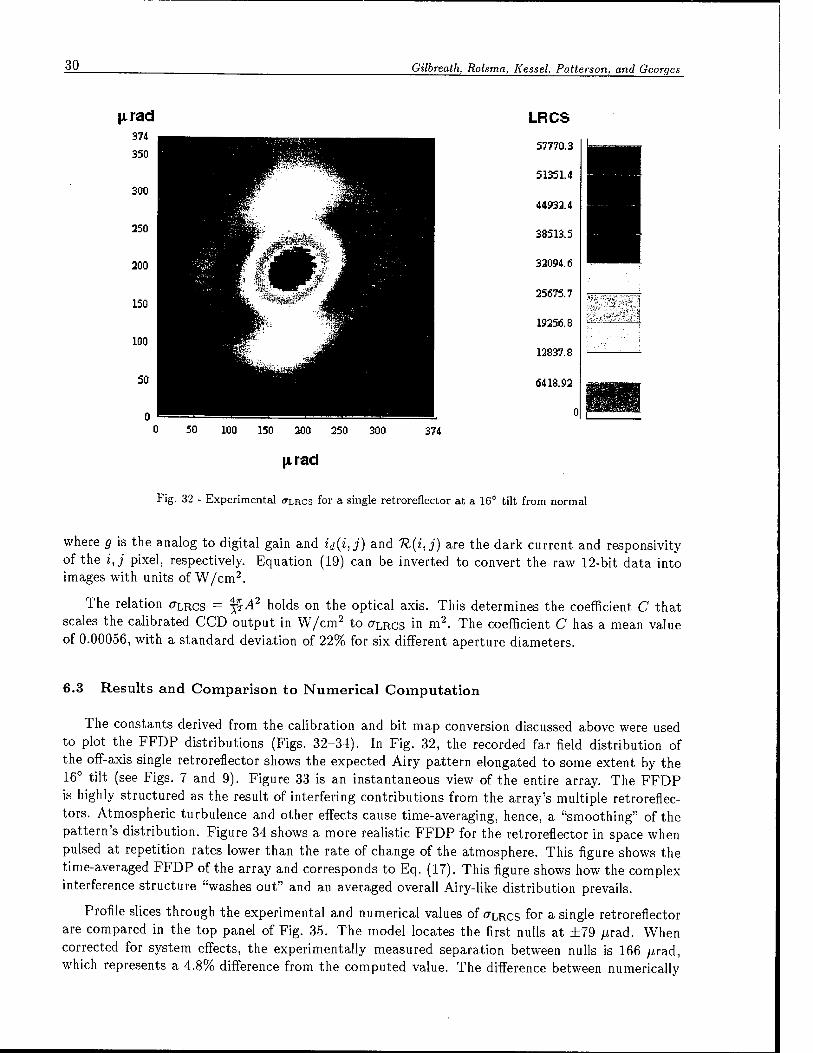
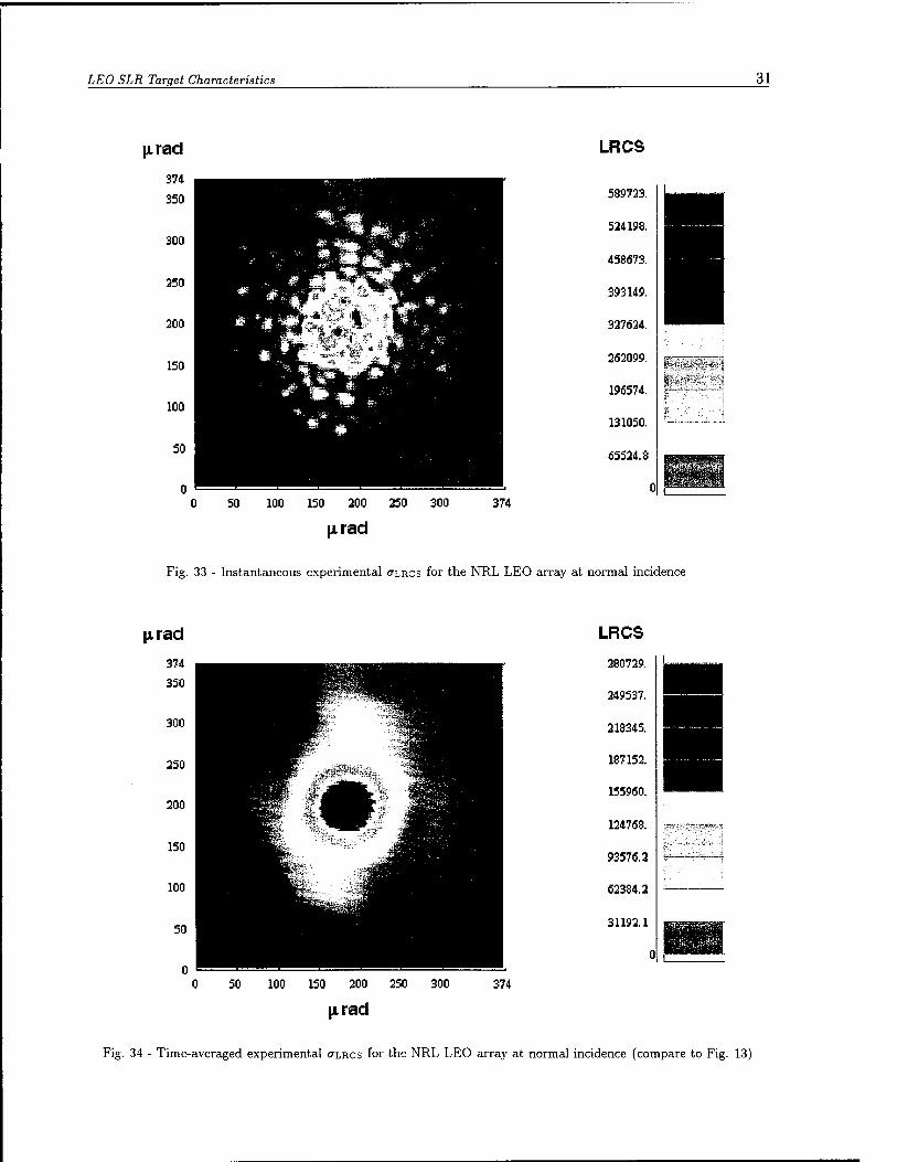
The constants derived from the calibration and bit map conversion discussed above were used to plot the FFDP distributions (Figs. 32-34). In Fig. 32, the recorded far field distribution of the off-axis single retroreflector shows the expected Airy pattern elongated to some extent by the 16° tilt (see Figs. 7 and 9). Figure 33 is an instantaneous view of the entire array. The FFDP is highly structured as the result of interfering contributions from the array's multiple retroreflec- tors. Atmospheric turbulence and other effects cause time-averaging, hence, a "smoothing" of the pattern's distribution. Figure 34 shows a more realistic FFDP for the retroreflector in space when pulsed at repetition rates lower than the rate of change of the atmosphere. This figure shows the time-averaged FFDP of the array and corresponds to Eq. (17). This figure shows how the complex interference structure "washes out" and an averaged overall Airy-like distribution prevails.
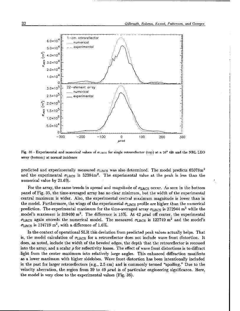
Profile slices through the experimental and numerical values of CTLRCS f°r a single retroreflector are compared in the top panel of Fig. 35. The model locates the first nulls at ±79 /trad. When corrected for system effects, the experimentally measured separation between nulls is 166 ^trad, which represents a 4.8% difference from the computed value. The difference between numerically
LEO SLR Target Characteristics 31
ixrad
374
350
300
250
200
150
100
50
♦5 #i'
& £? ■ ■
*-*4M
*
«ft, ..«.. .' W ■■©'
* 4 1
LRCS
589723.
524198.
458673.
393149.
327624.
262099.
196574.
131050.
65524.8
0 50 100 150 200 250 300 374
Israel
Fig. 33 - Instantaneous experimental ULRCS for the NRL LEO array at normal incidence
ixrad
0 50 100 150 200 250 300 374
l^rad
LRCS
280729.
249537.
218345.
187152.
155960.
124768.
93576.2
62384.2
31192.1
Fig. 34 - Time-averaged experimental CTLRCS for the NRL LEO array at normal incidence (compare to Fig. 13)
32 Gilbreath, Rolsma, Kessel, Patterson, and Georges
6.0x10
5.0x10
E 4.0x10^
3.0x10^
2.0x10
1.0x10
3.0x10
2.5x10-
2.0x10-
Ö 1.5x10-
1.0x10-
5.0x10^ r
1 -cm retroreflector
numerical experimental
— 22—element array numerical experimental
-300 300
Fig. 35 - Experimented and numerical values of CTLRCS for single retroreflector (top) at a 16° tilt and the NRL LEO
array (bottom) at normal incidence
predicted and experimentally measured CTLRCS was also determined. The model predicts 65078m2
and the experimental CTLRCS 1S 52384m2. The experimental value at the peak is less than the
numerical value by 21.6%.
For the array, the same trends in spread and magnitude of CTLRCS occur. As seen in the bottom panel of Fig. 35, the time-averaged array has no clear minimum, but the width of the experimental central maximum is wider. Also, the experimental central maximum magnitude is lower than in the model. Furthermore, the wings of the experimental CTLRCS profile are higher than the numerical prediction. The experimental maximum for the time-averaged array CTLRCS is 272944 m2 while the model's maximum is 319460 m2. The difference is 15%. At 42 ^rad off center, the experimental o'LRCS again exceeds the numerical model. The measured CTLRCS is 122749 m2 and the model's CTLRCS is 124719 m2, with a difference of 1.6%.
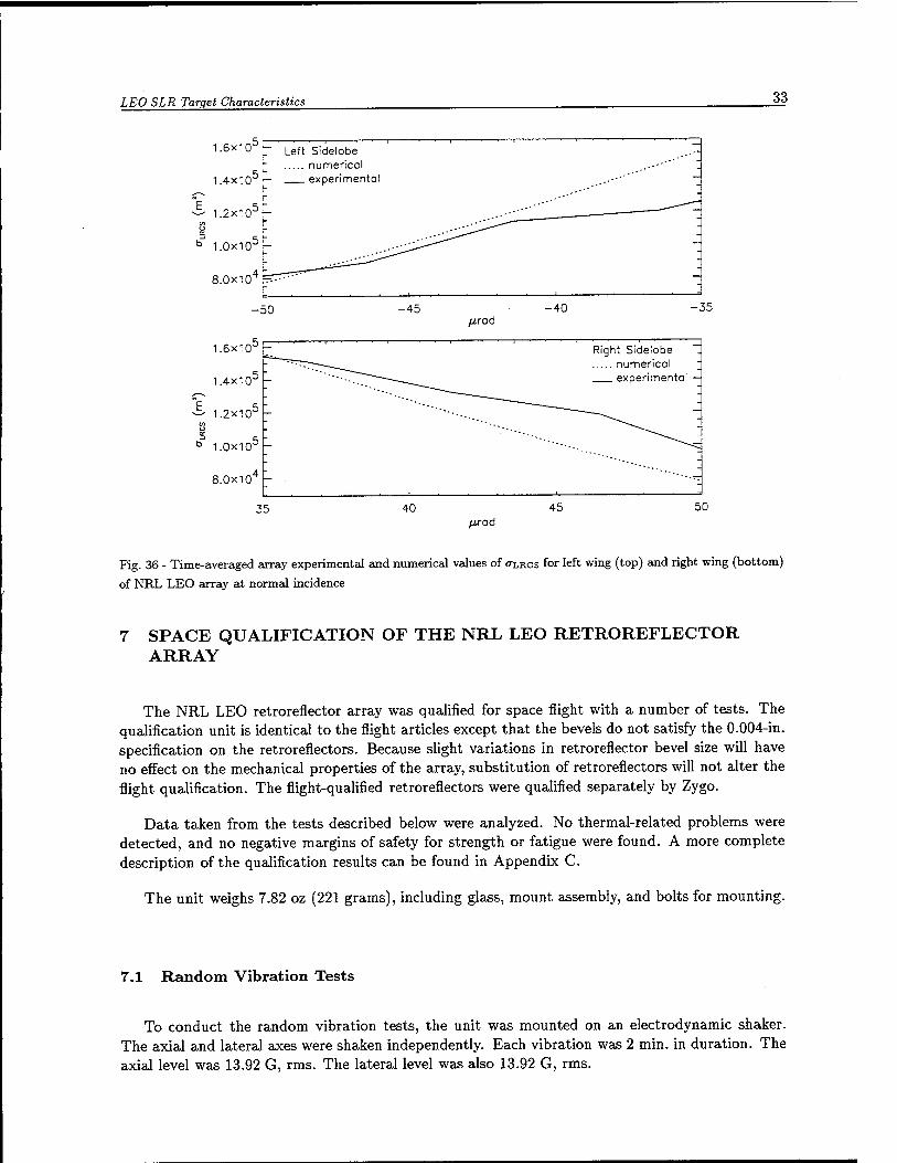
In the context of operational SLR this deviation from predicted peak values actually helps. That is, the model calculation of CTLRCS for a retroreflector does not include wave front distortion. It does, as noted, include the width of the beveled edges, the depth that the retroreflector is recessed into the array, and a scalar p for reflectivity losses. The effect of wave front distortions is to diffract light from the center maximum into relatively large angles. This enhanced diffraction manifests as a lower maximum with higher sidelobes. Wave front distortion has been intentionally included in the past for larger retroreflectors (e.g., 2.5 cm) and is commonly termed "spoiling." Due to the velocity aberration, the region from 39 to 49 ^rad is of particular engineering significance. Here, the model is very close to the experimental values (Fig. 36).
LEO SLR Target Characteristics 33
1.6x10"
1.4x10"
1.2x10'
b 1.0x10"
8.0x10^ =^
Left Sidelobe numerical experimental
-50 -45 -40 -35 /xrad
1.6x10"" -
1.4x10"
1.2x10J -
b 1.0x10"
8.0x10
Right Sidelobe numerical experimental
35 40 45 50
/xrad
Fig. 36 - Time-averaged array experimental and numerical values of OXRCS for left wing (top) and right wing (bottom)
of NRL LEO array at normal incidence
7 SPACE QUALIFICATION OF THE NRL LEO RETROREFLECTOR ARRAY
The NRL LEO retroreflector array was qualified for space flight with a number of tests. The qualification unit is identical to the flight articles except that the bevels do not satisfy the 0.004-in. specification on the retroreflectors. Because slight variations in retroreflector bevel size will have no effect on the mechanical properties of the array, substitution of retroreflectors will not alter the flight qualification. The flight-qualified retroreflectors were qualified separately by Zygo.
Data taken from the tests described below were analyzed. No thermal-related problems were detected, and no negative margins of safety for strength or fatigue were found. A more complete description of the qualification results can be found in Appendix C.
The unit weighs 7.82 oz (221 grams), including glass, mount assembly, and bolts for mounting.
7.1 Random Vibration Tests
To conduct the random vibration tests, the unit was mounted on an electrodynamic shaker. The axial and lateral axes were shaken independently. Each vibration was 2 min. in duration. The axial level was 13.92 G, rms. The lateral level was also 13.92 G, rms.
34 Gilbreath, Rolsma, Kessel, Patterson, and Georges
7.2 Thermal Vacuum Tests
The unit was mounted on a thermally controlled heat sink, and thermocouples were used to monitor and control temperature. The vacuum was less than 0.00001 torr. The unit was tested through 6 cycles from -100° C to +71° C.
7.3 Pyroshock Tests
The unit was mounted on an electrodynamic shaker and again the two axes where shocked independently in axial and lateral dimensions. The peak levels of shock were 6,000 Gs.
8 CONCLUSIONS
Based on the analysis and experimental verification presented in this report, we conclude that the NRL LEO retroreflector array will robustly close a link from a standard 1,100-km circular orbit using an SLR system comparable to NASA's TLRS above a 20° elevation angle for daytime and nighttime ranging. The array will also close a link for a system as modest as the FTLRS 13-cm aperture system in Caparia. In addition, when analyzed for the meter-class system to be installed at MRC in 2000, the link will be robust enough to support unambiguous ranging at even the lowest elevation angles, day and night, without the aid of an amplifier.
The array itself comprises 22 1-cm diameter retroreflectors situated on a hemisphere to produce a far field diffraction pattern that provides a laser radar cross section of greater than 104 m2 for elevation angles above 20° with a 108° FOV. It has a mass of 221 grams and measures 82 mm in diameter by 43 mm in height.
Analysis was verified by bench experiments and showed that manufacturing defects in the wave front quality of the retroreflector direct energy to a small extent into sidelobes. It was shown that these enhanced sidelobes help the link by compensating for velocity aberration.
Results were compared to the predicted performance of a single cube. It was shown that the FOV would be severely restricted when using one cube, hence orbital sampling would be significantly reduced.
Predicted performance in the near-infrared at 1064 nm was also presented. Advantages of this wavelength include better transmission through the atmosphere and covertness due to transmission in the nonvisible region of the spectrum.
The array was space-qualified, and testing specifications are detailed in Appendix C.
ACKNOWLEDGMENTS
Mark Davis (NRL Code 8123/Allied Signal) provided the ephemeris and attitude data for all passes above the Washington, D.C. area. Data for the TOPEX/Poseidon passes over Capraia are the work of Jim Barnds (NRL Code 8233). We gratefully acknowledge both of their efforts in support of this report.
LEO SLR Target Characteristics 35
ACRONYMS
APD avalanche photodiode
COM center of mass
FAA Federal Aviation Administration
FFDP far field diffraction pattern
FOV field of view
FTLRS field-transportable laser radar station
FWHM full-width at half maximum
LEO low Earth orbit
LRCS laser radar cross section (or CTLR.CS)
MOBLAS mobile laser ranging system
MRC Midway Research Center
NRL Naval Research Laboratory
OPC optical phase center
PCA point-of-closest approach
SLR satellite laser ranging
SOR Starfire Optical Range, Kirtland AFB, New Mexico
TLRS transportable laser ranging system
REFERENCES
[1] G.C. Gilbreath, P.W. Schumacher Jr., M.A. Davis, E.D. Lydick, and J.M. Anderson, "Cali- brating the Naval Space Surveillance "Fence" Using Satellite Laser Ranging Data," Proceedings of the 1997 AAS/AIAA Astrodynamics Specialist Conference 97, 1997.
[2] J.J. Degnan, "Millimeter Accuracy Satellite Laser Ranging A Review," Contributions of Space Geodesy to Geodynamics Technology 25, 133-162 (1993).
[3] A.R. Peltzer, G.C. Gilbreath, G.E. Price, and W.J. Barnds, "Ephemeris Estimation of a Well- Defined Platform Using Satellite Laser Ranging from a Reduced Number of Ground Sites," NRL Report NRL/FR/8120-96-9800, April 1996.
[4] G.C. Gilbreath, M.A. Davis, P.B. Rolsma, R. Eichinger, T. Meehan, and J.M. Anderson, "Naval Research Laboratory at Starfire Optical Range: Satellite Laser Ranging with Robust Links," SPIE Aerosense 97, SPIE 3065-51, 1997.
36 Gilbreatk, Rolsma, Kessel, Patterson, and Georges
[5] P.O. Minott, "Design of Retrodirector Arrays for Laser Ranging of Satellites," NASA TM-X- 723-74-122, Goddard Space Flight Center, Greenbelt, Md., March 1974.
[6] RO. Minott, "Measurement of the Lidar Cross Sections of Cube Corner Arrays for Laser Ranging of Satellites," NASA TM-X-722-74-301, Goddard Space Flight Center, Greenbelt, Md., September 1974.
[7] M. Born E. Wolf, Principles of Optics, 6th ed. (Pergamon Press, Oxford, 1985), pp. 395-398.
[8] J.W. Goodman, Introduction to Fourier Optics, 2nd ed. (McGraw-Hill, New York, 1996), pp. 63-78.
[9] G.C. Gilbreath, P.B. Rolsma, and R. Kessel, "Analysis of SLR Targets for JASON," NRL Memorandum Report 7971, August 1997.
[10] J.H. Churnside, "Turbulence Effects on the Geodynamics Laser Ranging System," NOAA Technical Memorandum ERL WPL-218, January 1992.
Appendix A
DIFFRACTION PATTERN AND PASS GEOMETRY CALCULATIONS
A.l Circular Retroreflector Far Field Diffraction Patterns
A convenient method to develop the analytic basis for the numerical determination of far field diffraction patterns begins with the simplest case and then adds refinements. With this approach, numerical implementation of each stage can serve as a limiting test case for the next stage. Our starting case is normal incidence without bevel losses; we finish with tilted incidence with bevel losses. As has been noted in the body of this report, introducing a tilt in the incidence direction is a much larger effect than are the bevel losses.
A. 1.1 Normal Incidence Without Bevel Losses
Consider a circular retroreflector with bevel loss regions directly overhead. The two-dimensional Fourier transform of the complex reflectance of the aperture, effectively the retroreflector's far field diffraction pattern Ä(x, y) is given by
ä(kx,ky) = ff dxdyÄ{x,y)e-ik**e-ikyy . (Al) J ./aperture
Using the function c(x) = \Jr2 - x2, which defines the top half of the circular aperture, the double integral can be rewritten as
fi^jfe,,) = f dxe-ik" fX e^Uy (A2) J—r J—c(x)
_ r e-ikXX_±_ \e-ikyC{x) _ eikyC(x)l dx (A3) J-r -iky L -I
_ T e~ikxx J_ Likyc(x) _ c-t*,c(*)l dx (A4) J—r 2fcv i- J
Ky J—r
y
-2i sin kyc(x) dx (A5)
2 f = — / [coskxx — ismkxx]sinkyc(x)dx (A6)
Ky J—r
— — I coskxxsin (kyy/r2 — x2) dx
— ■— / sin kxxsin [ky\/r2 — x2) dx . (A7)
kv J-r v '
37
38 Gilbreath, Rolsma, Kessel, Patterson, and Georges
When Eq. (A7) is integrated numerically, the absolute magnitude of ä(kx, ky) determined, and then converted to a cross section, the result is the azimuthally symmetric Airy function of Fig. 6. (See Section B.l for the numerical implementation of Eq. (A7).) The numerical routine that implements this geometry serves as a limit test case for the tilted and normal incidence with bevel losses routines.
A. 1.2 Tilted Incidence Without Bevel Losses
When a circular retroreflector is tilted, the aperture changes shape to the overlap region of two offset circles. The tilt away from normal incidence can be related to the circles' offset x0 from the center of the retroreflector. For a retroreflector of depth d with a face recessed by distance c and index of refraction n, the expression relating x0 to the angle 6inci between the surface normal and the incidence direction is
x0 = c sin 6inci + d sin 6n , (A8)
where
6n = arcsin sin 9;
(A9)
For a circular retroreflector of radius r, d = y/2r. The retroreflector's field of view (FOV) is limited by the requirement that x0 < r. For a 1-cm diameter retroreflector with n - 1.46 and c = 0.1016 cm (or 0.040 in.), the FOV cut off is at fl,^ = 58.579°. The aperture boundary for the tilted retroreflector is defined by c(x) = ±-s/r
2 - (x - x0)2 for x < 0 and c(x) = ±^r2 - (x + x0)2
for x > 0. The aperture's shape is that of a cat's iris or an American football profile shown in the upper panel of Fig. 8.
Integrating each side of the aperture separately yields a two-dimensional Fourier transform for tilted incidence with four integrals given by
ü[kXj Ky) 2_
j coskxxsin (kyyjr2 - (x - x0)2)dx
+ / cos kxx sin (ky^r2 - (x + x0)2 J dx
- — j sin kxx sin ( ky^Jr2 - (x - x0)2) dx
+ / sin kxx sin ( kyyjr2 - (x + x0)2 J dx (A10)
Equation (A10) yields a reasonable transform and limits to an Airy function as x0 -> 0. (See Section B.2 for the numerical implementation of Eq. (A10).) Figure 10 shows the sizable variation in the laser radar cross section of a tilted circular retroreflector as one sweeps kx and ky with a constant magnitude of k of 50 /xrad (i.e., roughly a satellite's velocity aberration for a 1,100-km high orbit).
A.1.3 Normal Incidence With Bevel Losses
Consider a circular retroreflector with bevel loss regions directly overhead. There are six regions, symmetric about the x-axis, that can be used to compute the two-dimensional Fourier transform for the aperture. These regions are shown in Fig. Al.
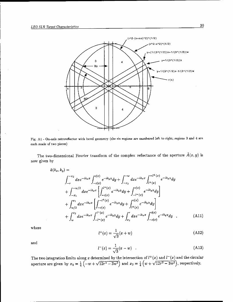
LEO SLR Target Characteristics 39
(rA2-(x+xo)A2)A(1/2)
(rA2-xA2)A(1/2)
y = (1/(3A(1/2))x + 1/(3A(1/2))w
y=1/(3A(1/2))x
y = 1/(3A(1/2)x-1/(3A(1/2)w
r(x)
Fig. Al - On-axis retroreflector with bevel geometry (the six regions are numbered left to right; regions 3 and 4 are
each made of two pieces)
The two-dimensional Fourier transform of the complex reflectance of the aperture A(x, y) is now given by
Q,{KX) Kyj
where
and
—w r—l^{x —ikxx /—X2 rc\x) f~w ., r
dxe~ik*x / e-tk»ydy + / dxe~lkxX / -r J-c(x) J-x2 Jl-
+ f~W 2 dxe~ikxX f
dxe~lKxX I e~ikyydy
+ / dxe~ikxX
lw/2 / e-,k>vdy +
J-c(x) JlJ
x2 Jl±(x)
c(x)
c(x) dy
I rx2 rl~(x) f tc
+ / dxe~ik*x / e~zkyydy+ / dxe~%kxX \ Jw J—l~(x) Jx2 J—
:(x)
■l-(x)
dy\
,-ikyV
l+{x) = ^{x + v)
1 ^ = 7f^-w)
dy (AH)
(A12)
(A13)
The two integration limits along x determined by the intersection of /+ (x) and I (x) and the circular aperture are given by xi = \ (-w + Vl2r2 - 3w2) and x2 = \ (w + y/l2r2 - 3w2J, respectively.
40 Gilbreath, Rolsma, Kessel, Patterson, and Georges
Rather than working with all six terms in Eq. (All) at once, the forms are reduced to be convenient for numerical integration individually. The six terms are:
/—X2 fc(x)
dxe~tk*x / e~%kyydy , ■r J—c(x) (x)
0.2 dxe~tk*x / e'^dy , -X2 Jl+(X) -X2
f—w/2 t—w/2 rl~(x) ., rc(x) ä3{kx,ky) = / dxe-tk" / e-xh**dy + \
J-xi [J-c(x) J-l-(x)
Ö4^rCx, Ky
-xi
fXl
,-ikyy
-c(x) dy
fXl \ f-l+{x) rc(x) = / dxe-tk'x / e-
tk»ydy + / , Jw/2 \J-c(x) Jl+(x)
-ikyy
I2
rx2
c(x)
l-(x)
dy
a5
rx2 ., /•' (x) (kx,ky) = / dxe-tk'x / e-
xk»*dy , Jw ->-l-(x)
and
~a6{kx,ky) = r dxe~ik*x fC X e~ikyydy Jx2 J—c(x)
(A14)
(A15)
(A16)
(A17)
(A18)
(A19)
Both äi{kx,ky) and ä6(kx,ky) have upper and lower limits defined by the circular aperture, as in Eq. (A2) for the integration along y. Hence, these two terms can be immediately simplified to the same form as Eq. (A7), yielding
O p—X2
äi(kx,ky) = — / coskxx sin (ky\/r2 - x2J dx
and
2z f~x2 , , , - — / sin kxx sin (ky yr2 - x2) dx ,
2 rr i . ä6(kx,ky) = — I cosA^xsin (kyy/r2 - x2) dx
fäy J X2
— — / sin kxx sin (kyy/r2 - x2) dx
(A20)
(A21)
Note, of course, that the x integration limits in Eqs. (A20) and (A21) are different than those in Eq. (A7). Similarly, ä2(kx,ky) and a5(kx,ky) can be reduced to integrals over x of the form
Q.2\kx, kyj 2 f~w f 1
— / cosA^xsin f ky —P(x + w) j dx Vy J-X2
2i f~W ( 1 + T- / sin kxx sin ( ky—^=(x + w) j dx ,
fcy J—X2 °
l
'7T (A22)
and
2 [X2 ( 1 \ ä5(fcr, A;,,) — — coskxxsin ( ky-y=(x - w))dx
2i [x* ( 1 \ — — / sin Ar^xsin ( ky—={x — w) j dx . (A23)
LEO SLR Target Characteristics 41
Note the sign change of the real and imaginary parts of Eq. (A22).
Simplifying a3(kx,ky) and ä4(kx,ky) can be done with the same approach. For ä4(kx,ky),
lw/2 e-ik»ydy
r-l+(x) fc(x)
J-c{x) Jl+{x)
1 Ukyl+(X) _ eikyC{x) + e-ikyC(x) _ g-ikyl+ix)'] fa -ik„ 1- J
rxi
Jw/2
= /
= fXl e~ikxX— \eik*cW - e~ikyC^ - eikyl+^ + e""***'"1'^] dx Jw/2 iky l
1 fXl rxi • r 1 1 I / e~,kxX -2i sin kyc(x) --2is,mkyl+(x)
ky Jw/2 U ">■
2 fXl
— — I [coskxx — isinkxx]smkyc(x)dx Ky Jw/2
2 fXl 4. — — / [coskxx — isinfc^a;] sin kyr (x)dx
ky Jw/2
= — < / cosfcxa;sin (ky\/r2 — x2) dx
ky [Jw/2 V '
— / cos kxx sin 1 ky—^=(x + w))dx>
- — < / sinfc^crsin \ky\/r2 - x2) dx
ky [Jw/2 V 7
- / sin kxx sin ( ky—j={x + w)\ dx> .
Finally, repeating these steps for a3(kx, ky) yields the similar form
r-w/2 ., f fl~(x)
dx
<*3
r-w 2 ft (x) rc{x) (kx,ky) = / «tee-*-* / e-%k**dy+ /
"' 7-an L"'-c(*) J-i-(x)
= — < / cosfcxa:sin (fc^vr2 — £2J <te
+ / coskxxsm {ky-j=(x — w)) dx>
— — < / sin fc^xsin (^\/r2 - a;2) <te
+ / sin kxx sin f ky—=(x — w)\ dx>
,—ifc; e~^ydy
(A24)
(A25)
(A26)
(A27)
(A28)
(A29)
(A30)
(A31)
The integrals in Eqs. (A20), (A21), (A22), (A23), (A29), and (A31) are to be evaluated numer- ically. Figure 12 shows the variation in the CTLRCS of a beveled circular retroreflector as one sweeps
4£ Gilbreath, Rolsma, Kessel, Patterson, and Georges
kx and ky with a constant magnitude of k of 50 yurad (i.e., roughly a satellite's velocity aberration). In comparison to the variation seen in Fig. 10, the bevels do not cause that much change in the magnitude, but they do introduce a six-fold symmetry.
A.1.4 Tilted Incidence With Bevel Losses
For a circular retroreflector with bevel loss regions, off-normal incidence angles tilted about the y-axis result in an aperture that is a combination of the cat's eye boundary and bevel loss regions. The position of the bevel loss regions is unchanged, and Eq. (A8) gives the correct offset in this case as well. Note that the FOV limit now becomes x0 < r - f. For a 1-cm diameter retroreflector with n = 1.46, c = 0.1016 cm (or 0.040 in.), and w = 0.01016 cm (or 0.004 in.), the FOV cut off is at 6inci — 57.63865°. Because the normal incidence case with bevel losses required distinct integration regions on each side of the aperture, the same six regions used for Eq. (All) can also be used in this case. The two integration limits along x determined by the intersection
of l+(x) and l~(x) and the aperture change to arx = § (- (\w + xQ) + ^/§r2 - \{w - x0)2\ and
X2 = I {(1^ ~ xo) + V 3r2 _ |(w + zo)2}, respectively. The two-dimensional Fourier transform for tilted incidence can be expressed in an analogous form to Eq. (All), where the resulting six terms are given by:
öi (kx, ky) = -— cos kxx sin ( kyyr2 - (x - x0)2 ] dx
- — / sin kxx sin ( kyy r2 - (x - x0)2 j dx , (A32)
2 f~w ( 1 \ ä2(kx,ky) — -7-/ coskxxsin i ky-j=(x + w)) dx
ky J-X2 V v3 /
2i f~w ( 1 \ + — / sin kxx sin I ky—j={x + w) 1 dx , (A33)
äz(kx, ky) = — I j cos kxx sin ( kyy r2 - (x - x0)2 ] dx
+ / coskxx sin f ky—j={x — w) 1 dx >
- -r- <, / sin kxx sin ( kyyjr2 - (x - x0)2 J dx
+ / sin fc^xsin f ky—j=(x - w) ) dx > , (A34)
ä4(kx, ky) = -j-\ coskxxsin ( kyy r2 - (x + x0)2 j dx
- / coskxxsm(ky—j=(x + w))dx>
- — < / sin kxxsin ( kyyr2 - (x + x0)2 ) dx
LEO SLR Target Characteristics 43
- / sinkxxsin(ky—~(x + w))dx> , (A35)
2 m / 1 \ ä5{kx,ky) = T- / coskxxsin \ky-T={x-w)\dx
/ sin kxxsin (ky-y=(x - w)\ dx , (A36) by
and
v
Kit
2 r(r~xo) / I -\ (kx,ky) = — coskxx sin i ky^r2 - (x + x0)2) dx
fcy Jx2 ^ '
1i r(r~xo) ( I \ sinkxxsinlkyyjr2 - (x + xo)2jdx . (A37) 2* r
f?7i Ja; y JZ2
Equations (A32) to (A37) limit properly to the untilted case as z0 -¥ 0. See Section B.3 for the numerical implementation of Eqs. (A32) to (A37).
A.2 Converting Pass Geometry to kxky Space
At a given instant, the orientation and velocity of the satellite with respect to the ground station determines the effective aperture of the retroreflector and the velocity aberration respectively.
For simplicity, consider a nadir-pointing retroreflector and use a fixed-Earth coordinate system. Hence, the ground station's location vector is a constant denoted by G, with fixed spherical coor- dinates of G, 0gs, and <j>gs. Note that 9gs is the ground station's colatitude measured down from the north pole rather than the latitude from the equator. The satellite's position is denoted by S, with spherical coordinates of 5, 0S/C, and <t>s/c. The satellite velocity v includes the effect of ground station motion. Finally, the range vector between satellite and ground station is R = S — G. Figure A2 illustrates the geometry and the local coordinate system at the satellite.
The angle of incidence 0inci, which defines the aperture through Eq. (A8), is the angle between S and R. Since G, S, and R form a triangle, 0inci can be related to the angular coordinates of G and S and the elevation angle 0eiev of the satellite at the ground site. The angle between G and S is given by
cos 7 = cos 0S/C cos 0gs + sin 0S/C sin 0gs cos(<j>s/c - <j>gs) . (A38)
Hence, Oelev + ~ + 7 + Qinci = * (A39)
or
In practice, the values of 0;nc; and 0eiev as a function of time during the pass are computed directly by orbital dynamics software. When working with a retroreflector array, 0inci is the angle between R and the array's axis. Hence, one must do a little further computation to determine the angle of incidence for each retroreflector with respect to R.
The apparent velocity of the retroreflector can be expressed in terms of velocity, ground station position, and satellite position. Once the velocity components in a satellite local coordinate system are determined, the values of kx and ky that define the ground stations position in the far field
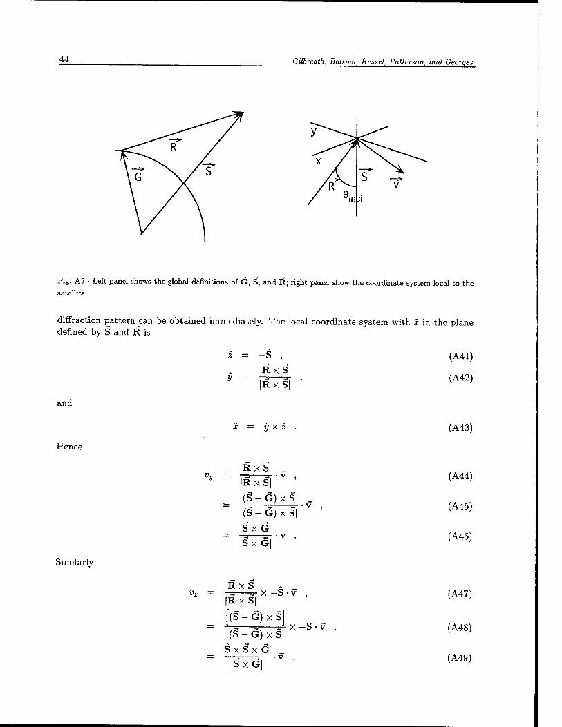
44 Gilbreath, Rolsma, Kessel, Patterson, and Georges
Fig. A2 - Left panel shows the global definitions of G, S, and R; right panel show the coordinate system local to the satellite
diffraction pattern j:an be obtained immediately. The local coordinate system with x in the plane defined by S and R is
and
Hence
y =
-s , RxS
IRx SI
y X z
vv = RxS _
|RxS| 'V '
(S-G)xS _
|(S-G)xS|'V
SxG ..
|Sx G| 'V
(A41)
(A42)
(A43)
(A44)
(A45)
(A46)
Similarly
vT = R x s A
-=r- X - -S- V |Rx S|
[(s- -G) x «] -S l(s- -G) x s| Sxi 3xG
• V ISXGI
(A47)
(A48)
(A49)
LEO SLR Target Characteristics 45
Finally,
- (T) (V) <-> and
'2TT\ f2v, k-={T){-f) ■ <A51>
The numerical routine to determine kx and ky from the results provided by the orbital dynamics group is a distinct module to simplify testing. (See Section B.4 for the numerical routine that determines kx and ky from the results provided by the orbital dynamics group.)
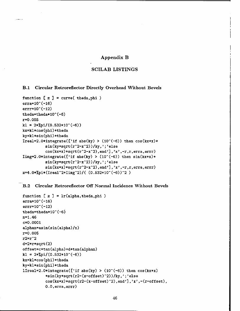
Appendix B
SCILAB LISTINGS
B.l Circular Retroreflector Directly Overhead Without Bevels
function [ z ] = curve( theda.phi ) erra=10-(-16) errr=10~(-12) theda=theda*10~(-6)
r=0.005
kl = 2*'/.pi/(0.532*10* (-6))
kx=kl*cos(phi)*theda
ky=kl*sin(phi)*theda
Ireal=2.0*integrate(['if abs(ky) > (10~(-6)) then cos(kx*x)*
sin(ky*sqrt(r~2-x~2))/ky,';'else cos(kx*x)*sqrt(r~2-x~2),end'],'x',-r,r,erra,errr)
Iimg=2.0*integrate(['if abs(ky) > (10~(-6)) then sin(kx*x)*
sin(ky*sqrt(r~2-x~2))/ky,';'else
sin(kx*x)*sqrt(r~2-x~2),end'],'x',-r,r,erra,errr)
z=4.0*,/.pi*(Ireal~2+Iimg~2)/( (0.532*10~(-6))"2 )
B.2 Circular Retroreflector Off Normal Incidence Without Bevels
function [ z ] = lr(alpha,theda.phi ) erra=10~(-16) errr=10~(-12) theda=theda*10~(-6)
n=1.46
c=0.0001
alphan=as in(s in(alpha)/n)
r=0.005
r2=r~2
d=2*r*sqrt(2)
offset=c*tan(alpha)+d*tan(alphan)
kl = 2*'/.pi/(0.532*10~(-6))
kx=kl*cos(phi)*theda
ky=kl*sin(phi)*theda
llreal=2.0*integrate(['if abs(ky) > (10"(-6)) then cos(kx*x)
*sin(ky*sqrt(r2-(x-offset)~2))/ky,';'else
cos(kx*x)*sqrt(r2-(x-offset)~2),end'],'x',-(r-offset),
0.0,erra,errr)
46
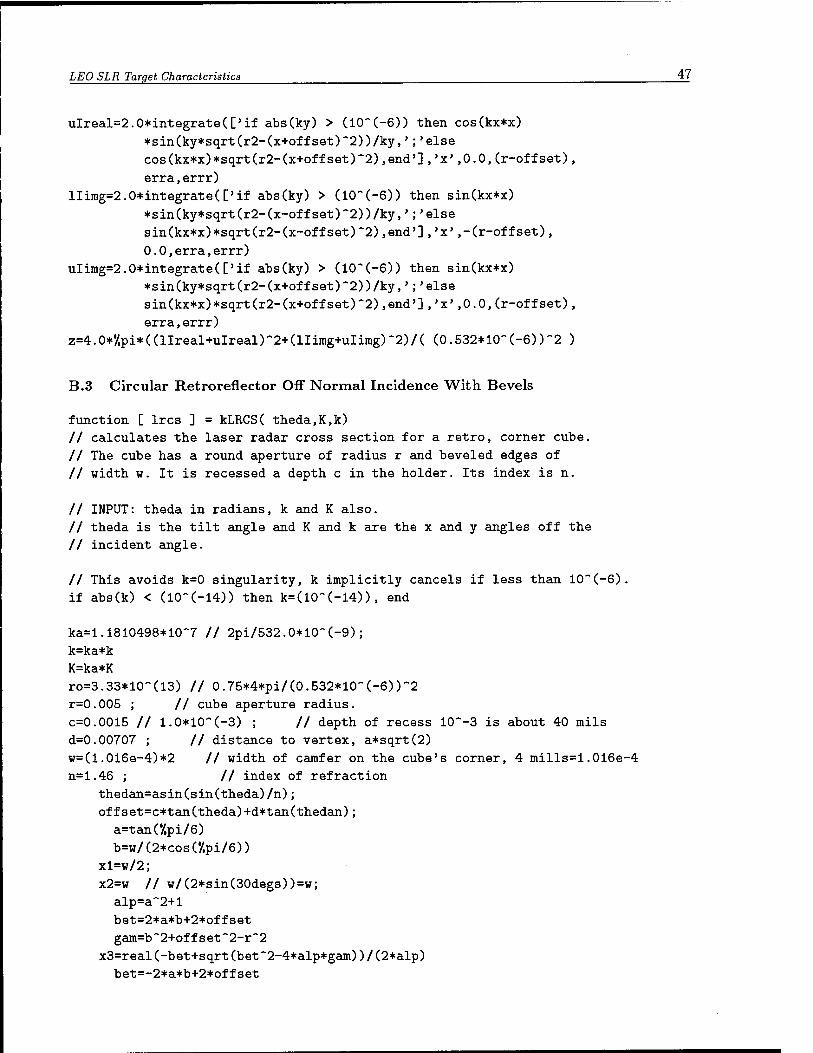
LEO SLR Target Characteristics 47
ulreal=2.0*integrate(['if abs(ky) > (10~(-6)) then cos(kx*x)
*sin(ky*sqrt(r2-(x+offset)"2))/ky,';'else
cos(kx*x)*sqrt(r2-(x+offset)"2),end'],'x',0.0,(r-offset),
erra,errr)
llimg=2.0*integrate(['if abs(ky) > (10"(-6)) then sin(kx*x)
*sin(ky*sqrt(r2-(x-offset)~2))/ky,';'eise
sin(kx*x)*sqrt(r2-(x-offset)"2),end'],'x',-(r-offset),
0.0,erra,errr)
ulimg=2.0*integrate(['if abs(ky) > (10~(-6)) then sin(kx*x)
*sin(ky*sqrt(r2-(x+offset)"2))/ky,';'eise
sin(kx*x)*sqrt(r2-(x+offset)~2),end'],'x',0.0,(r-offset),
erra,errr)
z=4.0*'/.pi*( (llreal+ulreal)"2+ (llimg+ulimg) "2)/( (0.532*10" (-6) ) "2 )
B.3 Circular Retroreflector Off Normal Incidence With Bevels
function [ Ires ] = kLRCS( theda,K,k) // calculates the laser radar cross section for a retro, corner cube.
// The cube has a round aperture of radius r and beveled edges of
// width w. It is recessed a depth c in the holder. Its index is n.
// INPUT: theda in radians, k and K also.
// theda is the tilt angle and K and k are the x and y angles off the
// incident angle.
// This avoids k=0 singularity, k implicitly cancels if less than 10"(-6).
if abs(k) < (10"(-14)) then k=(10"(-14)), end
ka=l.1810498*10"7 // 2pi/532.0*10"(-9);
k=ka*k
K=ka*K
ro=3.33*10~(13) // 0.75*4*pi/(0.532*10"(-6))"2
r=0.005 ; // cube aperture radius.
c=0.0015 // 1.0*10"(-3) ; // depth of recess 10"-3 is about 40 mils
d=0.00707 ; // distance to vertex, a*sqrt(2)
w=(1.016e-4)*2 // width of camfer on the cube's corner, 4 mills=l.016e-4
n=1.46 ; // index of refraction
thedan=asin(sin(theda)/n);
offset=c*tan(theda)+d*tan(thedan);
a=tan('/,pi/6)
b=w/(2*cosC/.pi/6))
xl=w/2;
x2=w // w/(2*sin(30degs))=w;
alp=a"2+l
bet=2*a*b+2*offset
gam=b"2+offset"2-r"2
x3=real(-bet+sqrt(bet~2-4*alp*gam))/(2*alp)
bet=-2*a*b+2*offset
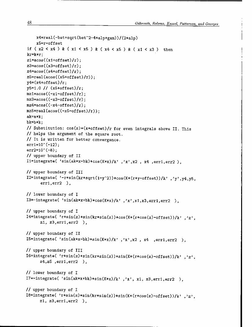
48 Gilbreath, Rolsma, Kessel, Patterson, and Georges
x4=real(-bet+sqrt(bet~2-4*alp*gam))/(2*alp) x5=r-offset
if ( x2 < x4 ) & ( xl < x5 ) & ( x4 < x5 ) & ( xl < x3 ) then kr=k*r;
zl=acos((xl+offset)/r);
z3=acos((x3+offset)/r);
z4=acos((x4+offset)/r);
z5=real(acos((x5+offset)/r));
y4=(x4+offset)/r;
y5=1.0 // (x5+offset)/r;
mzl=acos((-xl-offset)/r);
mz3=acos((-x3-offset)/r);
mz4=acos((-x4-offset)/r);
mz5=real(acos((-x5-offset)/r));
ak=a*k;
bk=b*k;
// Substitution: cos(z)=(x+offset)/r for even integrals above II. This // helps the argument of the square root.
// It is written for better convergence. errl=KT(-12); err2=lCT(-8);
// upper boundary of II
Il=integrate( 'sin(ak*x-bk)*cos(K*x)/k' ,'x',x2 , x4 ,erri,err2 ),
// upper boundary of III
I2=integrate( '-r*sin(kr*sqrt(l-y-2))*cos(K*(r*y-offset))/k' ,'y',y4,y5, errl,err2 ),
// lower boundary of I
I3=-integrate( 'sin(ak*x+bk)*cos(K*x)/k' ,'x',xi,x3,errl,err2 ),
// upper boundary of I
I4=integrate( 'r*sin(z)*sin(kr*sin(z))*cos(K*(r*cos(z)-offset))/k' ,'z', zl, z3,errl,err2 ),
// upper boundary of II
I5=integrate( 'sin(ak*x-bk)*sin(K*x)/k' ,,x',x2 , x4 ,errl,err2 ),
// upper boundary of III
I6=integrate( 'r*sin(z)*sin(kr*sin(z))*sin(K*(r*cos(z)-offset))/k' ,'z', z4,z5 ,errl,err2 ),
// lower boundary of I
I7=-integrate( 'sin(ak*x+bk)*sin(K*x)/k' ,'x', xl, x3,errl,err2 ),
// upper boundary of I
I8=integrate( 'r*sin(z)*sin(kr*sin(z))*sin(K*(r*cos(z)-offset))/k' ,'z', zl, z3,errl,err2 ),
LEO SLR Target Characteristics 49
// upper boundary of -II ; -II is the left mirror image of II
I9=integrate( 'sin(-ak*x-bk)*cos(K*x)/k' ,,x',-x4 ,-x2 ,erri,err2 ),
// upper boundary of -III I10=integrate( 'r*sin(z)*sin(kr*sin(z))*cos(K*(r*cos(z)+offset))/k' ,'z',
mz5,mz4,err1,err2 ),
// lower boundary of -I Ill=-integrate( 'sin(-ak*x+bk)*cos(K*x)/k' ,'x',-x3 , -xl ,errl,err2 ),
// upper boundary of -I I12=integrate( 'r*sin(z)*sin(kr*sin(z))*cos(K*(r*cos(z)+offset))/k' ,'z',
mz3, mzi,errl,err2 ),
// upper boundary of -II I13=integrate( 'sin(-ak*x-bk)*sin(K*x)/k' ,'x',-x4 , -x2 ,errl,err2 ),
// upper boundary of -III I14=integrate( 'r*sin(z)*sin(kr*sin(z))*sin(K*(r*cos(z)+offset))/k' ,'z',
mz5,mz4,errl,err2 ),
// lower boundary of -I I15=-integrate( 'sin(-ak*x+bk)*sin(K*x)/k' ,'x', -x3, -xl,errl,err2 ),
// upper boundary of -I I16=integrate( 'r*sin(z)*sin(kr*sin(z))*sin(K*(r*cos(z)+offset))/k' ,'z',
mz3,mzl,erri,err2 ),
// combine all contributions Ires = (2)*(Il-I2+I3-I4+I9-Ii0+Ill-I12-y.i*(I5-I6+I7-I8+I13-I14+Ii5-I16) ),
else lrcs=0,end lrcs=ro*abs(lrcs*conj(Ires))
B.4 Conversion to kxky
mode(-l) // Program generates LRCS for passes found in sub directory passes.
// // cube init, cnum is the number of cubes to be considered. unix_w('date') cnum=22; print C/,io(2) ,cnum) // thada is the sperical angle from the z axis. // phi is the angle from the x axis. c=2.99*10*8 thada=2**/,pi;
cub=zeros(cnum,3);
50 Gilbreath, Rolsma, Kessel, Patterson, and Georges
phi=16*'/.pi/180;
for i=l:4,cub(i,i)=cos((i-l)*thada/4)*sin(phi);end
for i=l:4,cub(i,2)=sin((i-i)*thada/4)*sin(phi);end
for i=i:4,cub(i,3)=cos(phi);end phi=32**/.pi/180;
for i=5:12,cub(i,i)=cos('/.pi/8+(i-l)*thada/8)*sin(phi);end
for i=5:i2,cub(i,2)=sin('/,pi/8+(i-l)*thada/8)*sin(phi);end
for i=5:12,cub(i,3)=cos(phi);end phi=48**/.pi/180;
for i=13:22,cub(i,i)=cos((i-l)*thada/10)*sin(phi);end
for i=13:22,cub(i,2)=sin((i-i)*thada/10)*sin(phi);end
for i=13:22,cub(i,3)=cos(phi);end
// klrcs returns LRCS for one cube kLRCS(theda,kxc,kyc),532nm ;getf("./klrcs.sei","c");
// Rot generates the rotation matrix to move the array coordinates // to the cube coordinates.
// In function kLRCS from klrcs.sei the major axis of the cube aperture // is always the y axis.
// Rxc normalized is the major axis and is pi/2+phi , phi the rotation axis. // cos(pi/2+phi)=-sin(phi) deff(,[Rc]=Rot(R,c),,[
,Rcr=CR(2)*c(3)-R(3)*c(2);R(3)*c(l)-R(i)*c(3);R(l)*c(2)-R(2)*c(i)]'; 'n=sqrt(Rcr(i)*Rcr(l)+Rcr(2)*Rcr(2)+Rcr(3)*Rcr(3))'; 'if n == 0 then Rc=[l,0;0,i],
else Rc=[Rcr(2)/n,-Rcr(l)/n;Rcr(i)/n,Rcr(2)/n] ,end' ])
deff('[z]=cross(x,y)','z=[x(2)*y(3)-x(3)*y(2),x(3)*y(l)-x(i)*y(3), x(l)*y(2)-x(2)*y(i)]>)
// macros to extract data from pass geometry found in a file in passes/ deff('Cr]=r(i)','r=y(i,32)')
deff('[R]=R(i)','R=Cy(i,18),y(i,19),y(i,20)]') deff('[s]=S(i) \ >s=[y(i,6),y(i,7),y(i,8)]')
deff('[g]=G(i)','g=-[y(i,l2),y(i,i3),y(i,i4)]')
deff('[v]=V(i)','v=-[y(i,9),y(i,iO),y(i,il)]-[y(i,i6),y(i,i6),y(i,17)]') deff('[ele]=el(i)>,>ele=y(i,31)')
deff (' [t]=time(i)', 't=y(i,3)*3600+y(i,4)*60+y(i,5)')
//
// LRCSA returns the LRCS for the 22 cube array
//
deff('[Ira]=LRCSA(theda,kxa,kya,cub)',[ 'lra=0.0';
'R=[sin(theda),0,cos(theda)]';
'for i=i:cnum, c=[cub(i,1);cub(i,2);cub(i,3)]; kc=Rot(R,c)*[kxa;kya] ;
lra=lra+kLRCS(acos(cub(i,3)),kc(i),kc(2)); end'] ) // // get the data for passes
//
//
// Begin of main loop, reading in data from a different file //
for p=i:l,// filnum(l,i), This was for multiple passes. Option is abandoned, filename='lpm03234'
LEO SLR Target Characteristics 51
print ('/.io (2), filename) load(filename) // open file for output, time,Ires,elevation
funit=f ileOopen', 'array.dat', 'new')
ysize=size(y) // creating arrays for storing data for future use.
lc=zeros(22,ysize(l,l))
l=l:ysize(l,l) 1=1*0
kx=l ky=l t=l ele=t
vel=t ang=t slantr=t for j=i:ysize(l,i), // calculating the incident vector, normalized, and in the array coordinates
nR=R(j)/norm(R(j)) nS=S(j)/norm(S(j)) // z axis of the array is parallel to S, nadir pointing. Nza=cos(theda_inc)
Nza=-nR*nS' sintheda=sqrt(1-Nza~2) // Nadir case has Nza=l and ExS=0, nRxS= INF
if Nza < 1.0 then RxS=cross(R(j),S(j)); nRxS=RxS/norm(RxS); nV=V(j)/norm(V(j)); Nya=sintheda*(nRxS*nV); RxSxS=cross(RxS,S(j)); nRxSxS=RxSxS/norm(RxSxS); Nxa=sintheda*(nRxSxS*nV'); Ninc=[Nxa,Nya,Nza] ; else Ninc=[0,0,1],end;
// V perpendicular to the direction of incidence
VxR=cross(V(j),R(j))/norm(R(j)); Vp=norm(VxR); // va, velocity aberation
va=2*Vp/c vel(j)=va // project each cube on to the plane perpendicular to R then calculate Ires
// test one nadir pointing cube for i=l:cnum,
Nc=[cub(i,l),cub(i,2),cub(i,3)];
theda=acos((Ninc*Nc')); // The next is parallel to the cubes y axis
yc=cross(Ninc,Nc) Nyc=yc/norm(yc) vay=va*Nyc(l) vax=va*Nyc(2)
kx(j)=vax ky(j)=vay ang(j)=theda
if theda < 0.9 then lc(i,j)=kLRCS(theda,vax,vay),end
Kj)=l(j)+lc(i,j) ,end
ele(j)=y(j,31) t(j)=time(j)
slantr(j)=norm(R(j)) // End of loop for one pass ,end
// write time,elevation, and Ires to a file
for j=l:ysize(l,l),Write(funit,Ct(j),l(j),ele(j),slantr(j)],'(4el2.5)'),end file("close",funit)
// save Ires for each point/cube save('221rcs',1c)
save('22t',t)
save('22ele',ele) save('22range',slantr)
xsetech([0,0,1.0,0.5])
plot(t.l) xtitle('LRCS vs time')
xsetech([0,0.5,1.0,0.5]) plot(t.ele)
xtitle('Elevation vs time') xsetech([0,0,1.0,1.0]) pca=0.0
for ipca=l:ysize(l,i),
if pea < y(ipca,31) then pca=y(ipca,31),
date='September '+string(y(ipca,l))+','+string(y(ipca,2))+' '+string(y(ipca,3))+':'+string(y(ipca,4))
,end,end
scmim=string(cnum)
title=string(pca)+' degree PCA'+' '+date+' c.number '+scnum xtitle(title) // End of main loop ,end
unix_w('date')
52
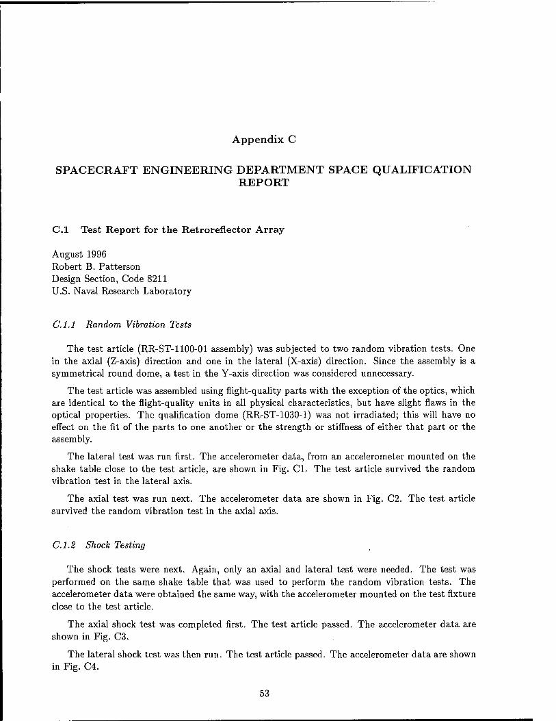
Appendix C
SPACECRAFT ENGINEERING DEPARTMENT SPACE QUALIFICATION REPORT
C.l Test Report for the Retroreflector Array
August 1996 Robert B. Patterson Design Section, Code 8211 U.S. Naval Research Laboratory
C.l.l Random Vibration Tests
The test article (RR-ST-1100-01 assembly) was subjected to two random vibration tests. One in the axial (Z-axis) direction and one in the lateral (X-axis) direction. Since the assembly is a symmetrical round dome, a test in the Y-axis direction was considered unnecessary.
The test article was assembled using flight-quality parts with the exception of the optics, which are identical to the flight-quality units in all physical characteristics, but have slight flaws in the optical properties. The qualification dome (RR-ST-1030-1) was not irradiated; this will have no effect on the fit of the parts to one another or the strength or stiffness of either that part or the assembly.
The lateral test was run first. The accelerometer data, from an accelerometer mounted on the shake table close to the test article, are shown in Fig. Cl. The test article survived the random vibration test in the lateral axis.
The axial test was run next. The accelerometer data are shown in Fig. C2. The test article survived the random vibration test in the axial axis.
C.l.2 Shock Testing
The shock tests were next. Again, only an axial and lateral test were needed. The test was performed on the same shake table that was used to perform the random vibration tests. The accelerometer data were obtained the same way, with the accelerometer mounted on the test fixture close to the test article.
The axial shock test was completed first. The test article passed. The accelerometer data are shown in Fig. C3.
The lateral shock test was then run. The test article passed. The accelerometer data are shown in Fig. C4.
53
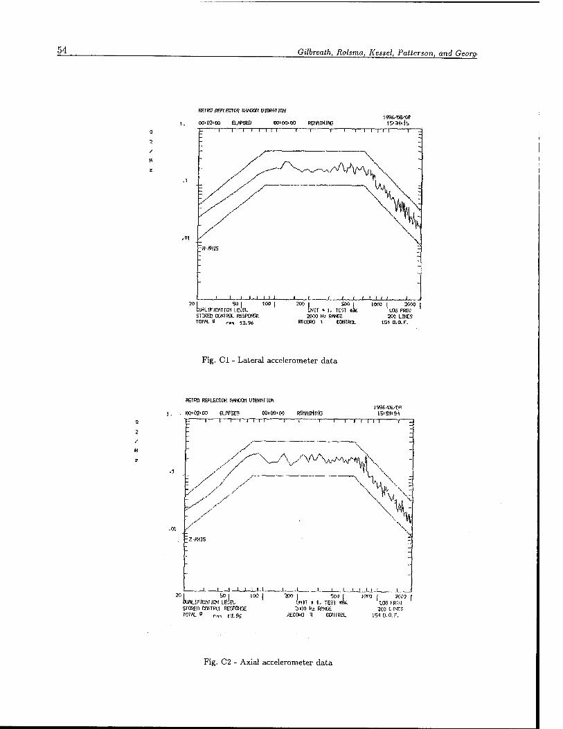
54 Gilbreath, Rolsma, Kessel, Patterson, and Georg:
trntso REFLECT« moon vtammm
00103> CO ELAPSED CO'00'00 RB1MN1NG 199<W03
15134^5 ~1 ~1 1—I 1 II ~I 1 1 IT I I I" "T ~T~
FM-«;s
j L_J 1—1—I, I I _u ,.i ___i ( i ,(,/,,„,. ■J, J
OUAUFlOVriCN LBKL ST0RQ3 CONTROl. RESPONSE T01«. 0 rM 13-%
200 UNIT «1, TEST III
2000 1000 I LOG reec
2000 Hi R«*E SCO LINES Rf.CORO 1 CONTROL ISi 0.0. F.
Fig. Cl - Lateral accelerometer data
RETRO REPLECtOR RflNMH UIETWT ION
1, . 00<02'00 HJV3E0 OOiOO'W REMftlNtrtj tS'S9i_4 —i—T—i—r-rrn—~T r—-i 1—i—r~r-rn r~™
/
/'
"V / A
/' /
J i.- _J._L.l_ 20 I 50 I 100 I
--«.JFffiWKW LEtS. SrtfiED ftOHTRa SESPOMS- 101PL 0 rm 13.94
,y'\^\^^-A/^\.K
\ H-\ x
1 .._.! 1 l.._.l_J__U..J JL. ..-_ »0 j 5C« j 1000 [ AC) |
UNIT » 1. T.SI »A4 ton (RSU 2000 It- RINGE 200 L PCS
RE.COSB 3 CtfflRm. IS1U.0.".
Fig. C2 - Axial accelerometer data
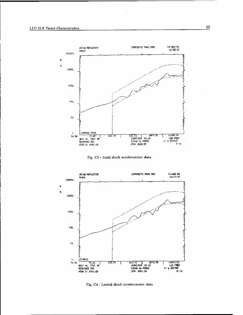
LEO SLR Target Characteristics 55
1030«.
ioooa.
1KB.
mea REFLECTOR- SHOCK
wo.
1. LaTBML AXIS 10.94 «.to I
UNIT H. 1KT »9' SESPCNSE SRi ras 6&&.S*
nmjSJTE HflKI »MX 13»52'02
/V
/.■-'
/" -i>
,-A7 v*''
«SS- S-T U3.H 2S73.S F 1C000.Ü0 DURATION 20.00 LOS FREU lOCao K* WW5E %.' 6 OCTA'JE ZW* «23.81 0 TO
Fig. C3 - Axial shock accelerometer data
100000.
10CO0.
10».
HEf?» REREETEF? CCrtWlTE Hfl«! MfiK
«.60 Wll «. "ESI «9' RESPONSE SRS PEAKS» <S7£>.H3
lisTST «62. IS I 253.;» 10000.00 OXffllON» 20.00 LOG FSED '10000 Hz RfifCE U «J OCTfME 3W <9S4.SÖ 0 to
Fig. C4 - Lateral shock accelerometer data
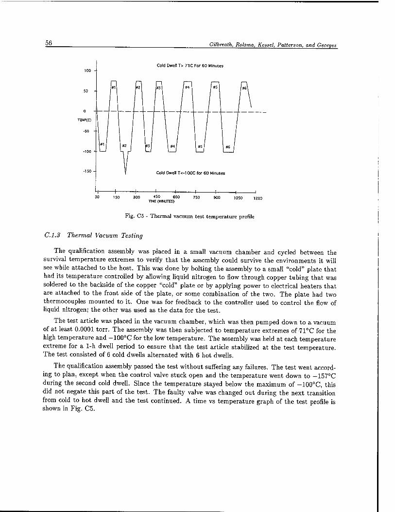
56 Gilbreath, Rolsma, Kessel, Patterson, and Georges
Cold Dwell T> 71C For 60 Minutes
300 4S0 600 TIME (MINUTES)
750 1050
Fig. C5 - Thermal vacuum test temperature profile
C.1.3 Thermal Vacuum Testing
The qualification assembly was placed in a small vacuum chamber and cycled between the survival temperature extremes to verify that the assembly could survive the environments it will see while attached to the host. This was done by bolting the assembly to a small "cold" plate that had its temperature controlled by allowing liquid nitrogen to flow through copper tubing that was soldered to the backside of the copper "cold" plate or by applying power to electrical heaters that are attached to the front side of the plate, or some combination of the two. The plate had two thermocouples mounted to it. One was for feedback to the controller used to control the flow of liquid nitrogen; the other was used as the data for the test.
The test article was placed in the vacuum chamber, which was then pumped down to a vacuum of at least 0.0001 torr. The assembly was then subjected to temperature extremes of 71°C for the high temperature and -100°C for the low temperature. The assembly was held at each temperature extreme for a 1-h dwell period to ensure that the test article stabilized at the test temperature. The test consisted of 6 cold dwells alternated with 6 hot dwells.
The qualification assembly passed the test without suffering any failures. The test went accord- ing to plan, except when the control valve stuck open and the temperature went down to -157°C during the second cold dwell. Since the temperature stayed below the maximum of -100°C, this did not negate this part of the test. The faulty valve was changed out during the next transition from cold to hot dwell and the test continued. A time vs temperature graph of the test profile is shown in Fig. C5.
LEO SLR Target Characteristics 57
C.2 Test Procedure for the Retroreflector Array
June 19, 1996 Robert B. Patterson Design Section, Code 8211 U.S. Naval Research Laboratory
C.Z.I Test Definition
C.2.1.1 Scope This document contains the requirements and procedures for the random vi- bration, shock, and thermal testing to be performed on the retroreflector array in order to qualify it for space flight on its host.
C.2.1.2 Test Objective The objective of this testing is to ensure that the retroreflector array is structurally sound and can withstand the launch and postlaunch environments without experiencing structural failure.
C.2.1.3 Pass/Fail Criteria
1. No parts (spring, retaining ring, retro seat, or retro optic) ejected from the assembly.
2. No noticeable permanent deformation around the seat area at the optic opening in the retrore- flector housing.
3. No noticeable permanent deformation around the retaining ring groove area of the retrore- flector housing.
C.2.1.4 Test Description Since the retroreflector assembly is a round part that is symmetrical about the axis of rotation, we will only have to test it in one longitudinal direction and the axial direction. We will mount the retroreflector assembly to the shaker table so that it is oriented for testing in the longitudinal direction. We will then run the test article through the 13.92 g rms random vibration test environment. We will then "hit" the test article with an extremely sharp impulse to simulate the shock environment (6000 g) specified by the host vehicle. We will now remount the retroreflector assembly so that it is oriented in the axial direction and repeat the random vibration and shock tests.
The thermal test consists of bolting the retroreflector assembly to a "cold" plate (that also has heaters installed on it), placing this assembly into a vacuum chamber, and then cycling the assembly through its survival temperature extremes six times.
C.2.1.5 Test Location The test will be conducted in the Naval Center for Space Technology's Payload Checkout Facility, Building A-59, at the Naval Research Laboratory in Washington, DC.
C.2.1.6 Responsibilities The Spacecraft Engineering Department is responsible for the over- all performance of the test, the data reduction, and production of the final test report.
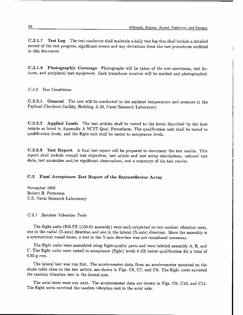
58 Gilbreath, Rolsma, Kessel, Patterson, and Georges
C.2.1.7 Test Log The test conductor shall maintain a daily test log that shall include a detailed record of the test progress, significant events and any deviations from the test procedures outlined in this document.
C.2.1.8 Photographic Coverage Photographs will be taken of the test specimens, test fix- tures, and peripheral test equipment. Each transducer location will be marked and photographed.
C.2.2 Test Conditions
C.2.2.1 General The test will be conducted in the ambient temperature and pressure in the Payload Checkout Facility, Building A-59, Naval Research Laboratory.
C.2.2.2 Applied Loads The test articles shall be tested to the levels described by the host vehicle as listed in Appendix A NCST Qual. Procedures. The qualification unit shall be tested to qualification levels, and the flight unit shall be tested to acceptance levels.
C.2.2.3 Test Report A final test report will be prepared to document the test results. This report shall include overall test objectives, test article and test setup descriptions, reduced test data, test anomalies and/or significant observations, and a summary of the test results.
C.3 Final Acceptance Test Report of the Retroreflector Array
November 1996 Robert B. Patterson U.S. Naval Research Laboratory
C.S.I Random Vibration Tests
The flight units (RR-ST-1100-01 assembly) were each subjected to two random vibration tests, one in the radial (Z-axis) direction and one in the lateral (X-axis) direction. Since the assembly is a symmetrical round dome, a test in the Y-axis direction was not considered necessary.
The flight units were assembled using flight-quality parts and were labeled assembly A, B, and C. The flight units were tested to acceptance (flight) levels 6 dB below qualification for a total of 6.92 g rms.
The lateral test was run first. The accelerometer data, from an accelerometer mounted on the shake table close to the test article, are shown in Figs. C6, C7, and C8. The flight units survived the random vibration test in the lateral axis.
The axial tests were run next. The accelerometer data are shown in Figs. C9, CIO, and Cll. The flight units survived the random vibration test in the axial axis.
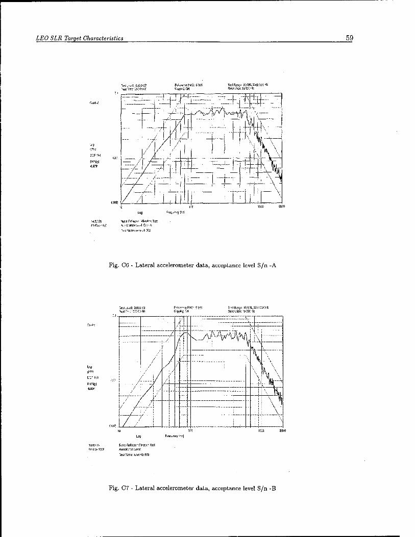
LEO SLR Target Characteristics 59
to
-.K-~ii:e.u;:>ä9 TalriT.5-CiKJii«
n»*i«o fiMS: 6.sS( Tstnsi;.; ic,i;cc,yj».»;* itowV cir. Vj D:C it
T7TR=" :h.
-~: £ '/
^~V*4/X JVo^;'
r~r
ib
pfc-k
' z_ 1$ K<£ &*>
;»o---o.-:i-s
r.|-Hj.."jJ? V;*fancslsv«l S.iv.',
Fig. C6 - Lateral accelerometer data, acceptance level S/n -A
fiü.
6.äJ<:
lest Level: iXWJ:i3 ':'l>(iitij 'Ji Res.
ri;p.; OSOHJ
!. ■ * \
:
! !
/' x^^ \ ; / •i
\N .,' / / /■■:- / i
'■■ Hi / i '"
V / /_/ /
fiV
lag
;t!-Uz* KZf tjxKt.:s£t>UXtA
Tcs) ?küi c: f<1n:ve.-.'W3
Fifcu.my ;'-s)
JCÜC 23W
Fig. C7 - Lateral accelerometer data, acceptance level S/n -B
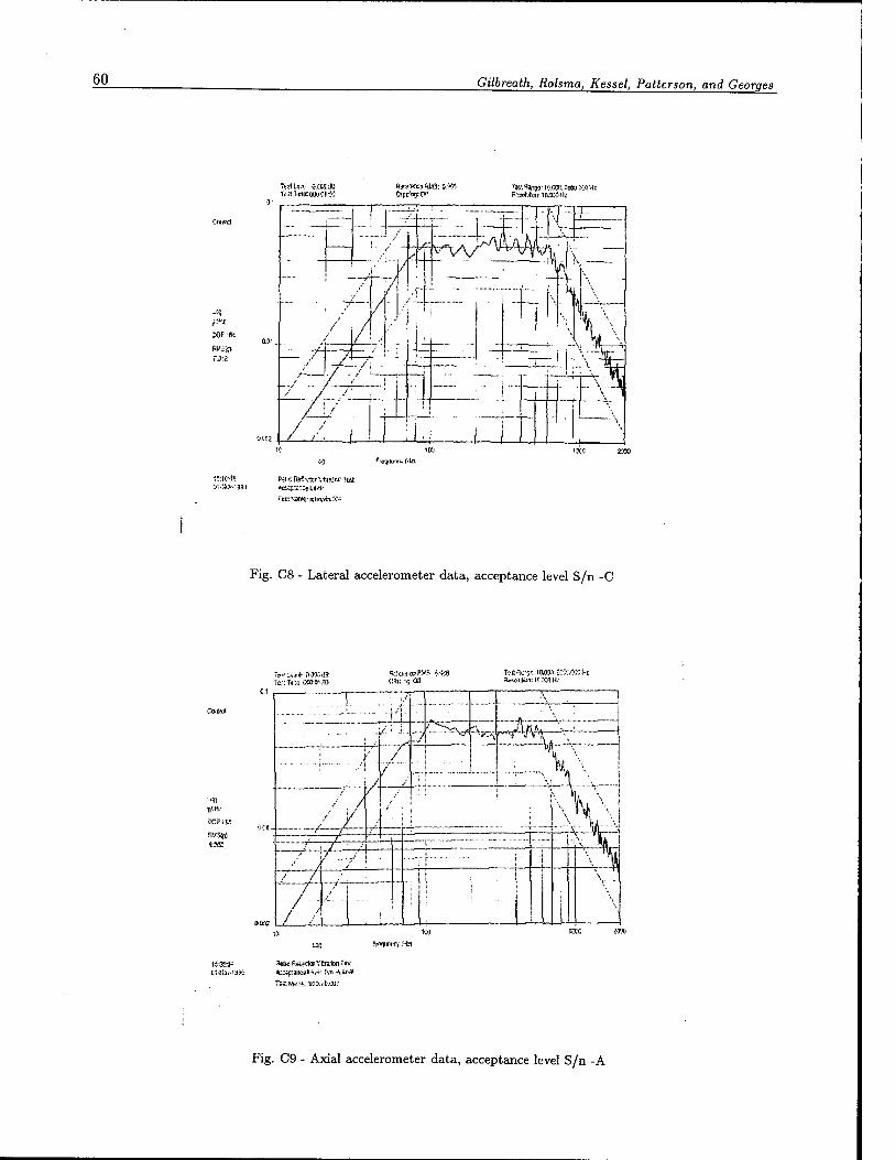
60 Gilbreath, Rolsma, Kessel, Patterson, and Georges
:or-k
FIO^IUI'I.'.". (Via
15:10* P4te R)9v!crV!b(ar« lut ir .;fcu.' 9911 »CLCj:^:* L>«
■3' l::HT!mo:tiU(JC)r>3
«*vwxs WJ3: 3:>w Clpc'ng: C«
'»tRUTjB-B.OTHaiCOä'.O-Hl FaobtarmKCrlz
, ' ~ '— _, ;\f -+-■ ...
1 ^^ . .MtliLlV >.
ji... •.
NV
•44-- - — —A >■■ /
as- _
— ^<
/
A / / 1/ i
.... \
— /ffl / .. r __— i —~-
—/ / ,-'..., / / ,■
; : i - \^ /' : : j
/ !/ , \
LJ — co? ■
/ / i in i 1
1K5 2333
Fig. C8 - Lateral accelerometer data, acceptance level S/n -C
tf.Hi
FKSM
O'r.TCrwBVS »I'M To*ac5C 10,03). JKCM+t
X—i-
T, /
/ /
7=
-7^ ■■■■ \r -\ •Vter-^
NL \
W\
KW 2M0
Trr.N&Ti.rwivt.CUi*
Fig. C9 - Axial accelerometer data, acceptance level S/n -A
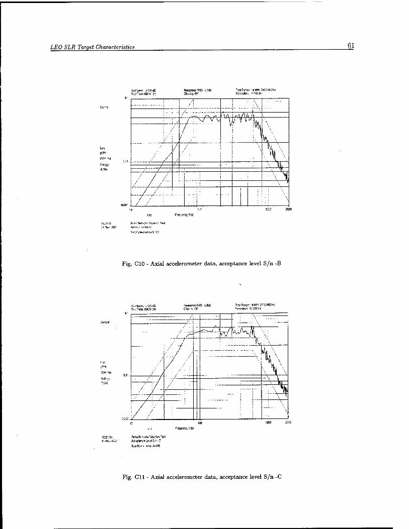
LEO SLR Target Characteristics 61
Liri
P.VSM
s -CM». • -.V*S»H.
-X'J.MOHr
) ,» ....
/ 1 A *fi/Ui j\ / : -\j v v >., ,» V^ftu
s "■• / 1 n
y
/; j \
\\ \ / v- u ,* . / / ■ \ i
■■'" / /
x 1 -., r : —7~T \
O.CCT „ f / r
1 "%
i«; «co
Fig. CIO - Axial accelerometer data, acceptance level S/n -B
3^"
.ft». 5 «C-.U0CH1
. ;/; .'- f -. ;
. ■ i , f \, Li',
/ /-"' ev \ !
■' : /
/ / / : .- :
L
1)}! •K /
...::r7i:::; "
,'i / / ; ; ■■■- i. / ! / : / ■• Hl \'S - / "
*-:-— /i / / 1
\ "i
/ : . / /: \
...
rrequrRy i.Ha
Trfff Hi--» *Kst.Yii »OS
Fig. Cll - Axial accelerometer data, acceptance level S/n -C
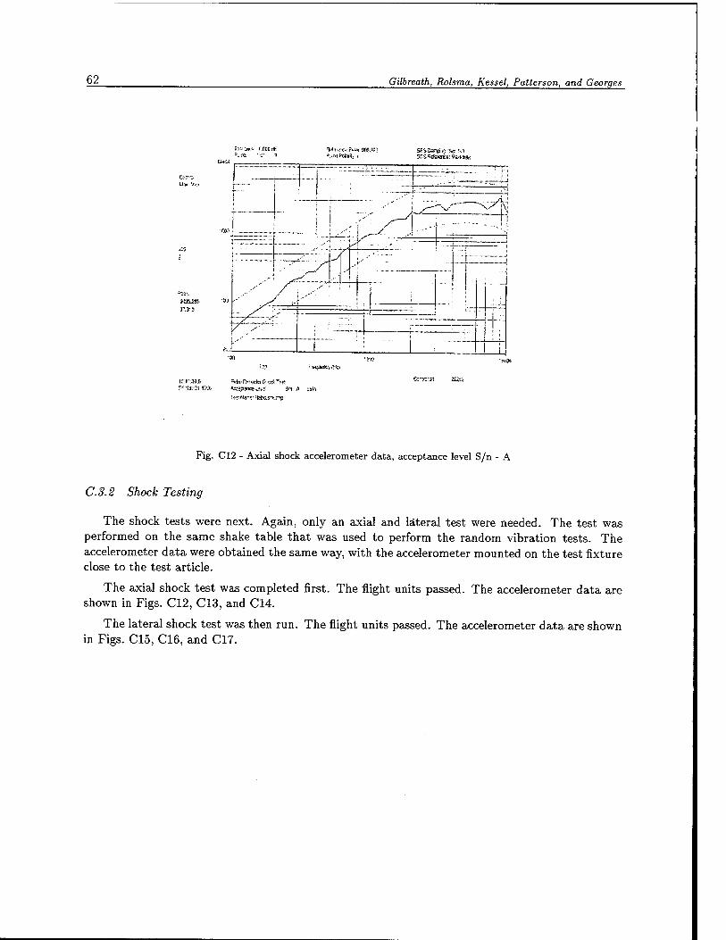
62 Gilbreath, Rolsma, Kessel, Patterson, and Georges
fracas Y&7
I---
^
^
r-Sj.-vMva srei-sancs-v:-: s^ A sah
Fig. C12 - Axial shock accelerometer data, acceptance level S/n - A
C.3.2 Shock Testing
The shock tests were next. Again, only an axial and lateral test were needed. The test was performed on the same shake table that was used to perform the random vibration tests. The accelerometer data were obtained the same way, with the accelerometer mounted on the test fixture close to the test article.
The axial shock test was completed first. The flight units passed. The accelerometer data are shown in Figs. C12, C13, and C14.
The lateral shock test was then run. The flight units passed. The accelerometer data are shown in Figs. C15, C16, and C17.
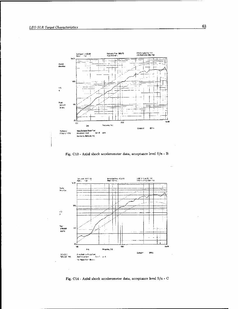
LEO SLR Target Characteristics 63
SRSRatsrM»:M»''-?n«t
—:::„ .:.... ' ■ ' '■ - ~1 ;'.. f ; ■ } \_ ■ ^H- '_JXZ^—TT7 t'l Ua»<tt« —■--—■—■ ■ f ■■ !■
iF *
CwttMl ZBfe 133« Ji 5<S3 Rates'9ra*TiW
Fig. C13 - Axial shock accelerometer data, acceptance level S/n - B
ft*.-.; 1 d Pute =•*:'>:, SHS£Vr:n;[>tt 5.C
OTCKB
t" ■ .., .
;' -v y\
. :-.•'„ _^z"" %/
.,■■' ' /^ ..." ..... •~ --.;..
^" -Y
■ y
») /
/ <;>
.. ..:..
V) [
FP-qtBflcy (H=!
£ci3td P- 2225a
Fig. C14 - Axial shock accelerometer data, acceptance level S/n - C

64 Gilbreath, Rolsma, Kessel, Patterson, and Georges
T-;sl i.(f -ri: 0.033 ill SR3 a*tei<sra»: V-.»i-ii«i
... — -. . , - "
A
.■—r\y — -\x \ ■■■ ■ - . ;
>*" ■ . ^
■■
./"
V -•' X. ••' /.-
s"^-- ' ' /■■■''
T:-.(N:r:r=w->rr!.ri-r
M*>| 22Sa
Fig. C15 - Lateral shock accelerometer data, acceptance level S/n - A
ice*;-
TesfLs-v 0.000 dB l»W! ST.,1;Damp•-.''.;, f:
OWE-a 1 ; .„-•■V.i ■ ^ \
..-"".
i 'y' \ >\
X"i ..." -• ' '" !
!■'■' i- :.^~~\ 'p/ . ...:. ._. S a i-*' "I -..JOSi 1 ,s'
,_ ._L..--... -i i ^'
33?t,22 1ÖC
2C
,-'•"' !/^ '.']. 1 ; }
I ;: :<5*< / ~ rr* ! 1 J > : ■ H ^" ■ ' ■
■■*']! ;
"!. — • .-■-- ^-- i / ■' i i
"T~7 f ' '. /■ _..■• : i ! '< 1 ! i i
i
£.-*#$*! (ESs
Fig. C16 - Lateral shock accelerometer data, acceptance level S/n - B
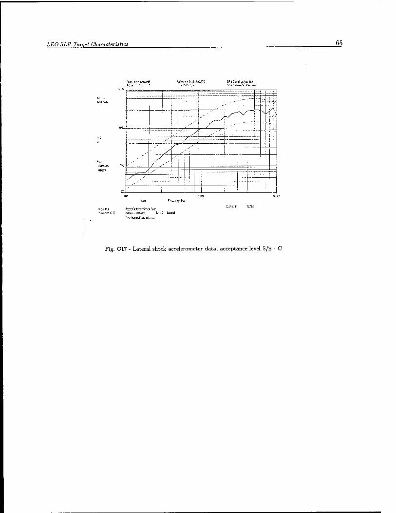
LEO SLR Target Characteristics 65
"n(jif,:C.<BJdB ä,:.-<- MB
il :9».?~o 3f Scampi;«« .5.5
,-■; ;-
^ ...-■ —
...... ~ ■ i .1:.
NTN
?cou_
i i
1 ^-
^Z ■.■<:=, s
1 / .':'
..■-•'■'
■
y .-■■' ■ ;
v' / ...
~ i
r-A^-q-J-JC
u;:- .r.t fer riefecte' S*>;k 7«; ^L',0.'^ trK- Ac:Kii:-:elev»' S.- -£ Laiaal
Fig. C17 - Lateral shock accelerometer data, acceptance level S/n - C