286Permanent income,redistribution and

income risk:Empirical analysison the role of age

and social protectionbenefits (ESSPROS)using Finnish Paneldata in 1995–2008

Ilpo Suoniemi

� � � � � � � � � � � � � � � � � � � � � � � � � � � � � � � �� � � � � � � � � � � � � � � � � � � � � � � � � � � � � � � � � � ! � � � � � � � � � " � " � � �

# $ % & ' ( ) ' * + , -. / 0 1 2 3 0 4 5 6 7 8 4 9 : 0 3 4 ; < ; : 0 = 4 > ; = 4 ? 5 > 5 1 ; = 0 3 0 4 4 ? 5 @ 0 A 9 7 3 / = > 4 ; 4 7 4 5 6 9 3 B < 9 = 9 1 ; < C 5 > 5 0 3 < ?D E 5 8 > ; = F ; G H I J K 6 9 3 7 > 5 6 7 8 < 9 1 1 5 = 4 > L M 7 = N ; = 2 6 3 9 1 O B @ P ; > 2 3 0 4 5 6 7 8 8 Q 0 < F = 9 R 8 5 N 2 5 N L. . / 8 : 9 L S 7 9 = ; 5 1 ; T 8 0 A 9 7 3 L U

V W X Y Z Y [ \ [ ] V Z ^ _ `a ] b c d b b ] e f Y Z Y [ \ b ^ _ `Y g h i g j k g g l m n j o p o i m q p k h g m o r kY m o i s j k m h h g j t g j o g u Z v w w x u w y n h k m j i mY p z { w | } ^ x u x ~ u u wb s z i � � r k o m � n o p j m q m { k p i p j m q m � h g � r p t { �� g � r p t ] j k o m o p o n � r t [ � r j r q m � \ n k n g t � zY m o i s j k m h h g j t g j o g u Z v � ] � w w x u w y n h k m j i m v � m j h g j �V n h n � z r j n � u x _ | ^ x u x ~ u u w[ � q g m h � � t k o j g q n { k p t j g q n � h g � r p t { �] b � f | ~ _ � | x ^ � ^ w | � � ^ w � _ � � � � �] b b f � ~ | x � � _ w � � � � � �

1

ABSTRACT

A large register based Finnish income panel data set with detailed information on the composition

of income over a 14 year time period, in 1995–2008 is used to examine income risk and

redistribution in the working age population, aged 20–59 years. In estimating relative risk premia in

factor and disposable income, the level of education, socio-economic status and age are controlled

for. The paper considers the extent of risk reduction due to the tax-benefit system which is

measured by differences between risk premia of equivalised factor and disposable household

income. The extent of risk reduction has decreased over the sample period. In the working-age

population, social protection benefits have a positive role in reducing the difference in risk premia

between factor income and disposable income while taxes have lost significance during the

observation period. In addition, certainty equivalent income concepts are utilised to get some

information on inequality in certainty equivalent income concepts and on redistribution of risk.

Young adults, 20–29 years old and elderly, near retirement age 55–59 years old, seem to benefit

most from social insurance. But all working age groups gain from redistribution in certainty

equivalent income relative to unadjusted redistribution of cash. Redistribution of income risk has

been reduced over the sample period. The findings are robust to a particular value of the degree of

risk aversion assumed.

Key words: risk-premium, inequality, redistribution, age

JEL classification: D31, D63, H24, H55, I31, J14

1. INTRODUCTION

Annual income distributions may give an incomplete and sometimes even distorted picture of

longer-term economic well-being. In a given year, people may have incomes which are transitorily

high or low for reasons such as unemployment, illness, good or bad luck, or exceptional economic

events. One of the primary motivations for economic mobility studies is to measure the extent to

which longer-term incomes are distributed more or less equally than incomes in a single year.

Shorrocks (1978) has emphasised: “Mobility is regarded as the degree to which equalization occurs

as the period is extended. This view captures the prime importance of mobility for economists.”

According to the above view, the recent rise in income inequality would be of less importance if it

2

had been accompanied with a rise in mobility.1 This suggests that one should not measure annual,

possibly transitory, change in inequality but the change measured over a longer (possibly life long)

time span.

Neoclassical welfare analysis which underlies most income distribution studies and public

economics is firmly anchored to static models under certainty. The analysis is somewhat lacking in

established views how to incorporate dynamics and evolving uncertainty into inequality studies and

models of optimal tax theory. How to introduce income mobility as an equalizer of longer term

income into the social objective function (Fields 2010)? Have prospects of mobility some special

merit over and above a mere comparison of static longer term (life cycle) income distributions?

More generally, income mobility may be viewed as a coin with two sides (Fields & Ok 1999). On

one hand, mobility may reduce long term inequality. On the other hand, mobility means fluctuations

in individual incomes. The shift in assessment from annual to multi-period inequality means that

future uncertainty about incomes must be accounted for in the evaluation (Creedy & Wilhelm

2002). Faced with less than perfect capital markets, forward-looking, risk-averse economic agents

view rise in income fluctuations as an increase in income risk which lowers economic well-being in

comparison with a steady flow of income. Therefore, interest in mobility also raises the issue of

predictability, or uncertainty. Uncertainty related to income fluctuations is a key dimension of

income mobility. A completely mobile society would mean complete economic insecurity. How to

combine income mobility both as an equalizer of longer term income and as an income risk

modifier into a well-defined social objective function (Creedy & Wilhelm 2002 and Fields 2010)?

Economic welfare and inequality have many dimensions, wages, earnings, income and final

consumption. Variability in, say, wages, is mediated by implicit social insurance and multiple

mechanisms of self-insurance. First, the household can adjust supply of working hours. Second,

joint earnings of the household are affected by public policies, progressive taxation, social

insurance and transfers. Third, informal contracts and voluntary gifts between households lend

added insurance. Fourth, the household can draw on their accumulated assets to temporarily finance

consumption. Furthest in line are partial adjustments in replacements of durable goods and semi-

1 In Finland annual income inequality rose significantly during the latter part of the 1990s (Riihelä, Sullström & Tuomala 2007, 2010). The period of major income equalization from mid 1960s to the mid 1990s has been reversed, taking the annual values of the Gini coefficient back to the levels of inequality found 40 years ago. In the Finnish case the phase of increasing income inequality has occurred much later than in the United States and in the United Kingdom, where annual income inequality has widened since early 1980s. In some other countries, such as Germany and Japan, the increase up to the early 1990s has been more modest, and Canada, France and Italy show no overall rise over the same period (Atkinson 2000).

3

durables. The last mechanism is particularly relevant for poor households often in the absence of

simple credit market.

The present paper looks at the income risk and inequality of longer term certainty equivalent

incomes which have been controlled for the undesirable effects of income fluctuations over time.

What is the pattern of Finnish income risk? Has there been a change in permanent income

inequality as annual income inequality has increased, and has the income risk been affected? How

much income insurance does government provide? Are individuals of different age in the same

situation? The paper illustrates how income panel data can be used to shed light on these and

similar questions. In particular, the paper highlights that part of income smoothing which is

provided by implicit social insurance rather than that affected by self-insurance (see also Carroll

1994, Carroll & Samwick 1998, and Hoynes & Luttner 2011).

The paper examines the dynamic income process of three different time periods in Finland, 1995–

1999, 2000–2004 and 2004–2008 with large panel data sets of Finnish working age population, 20–

59 years old. Relative risk premia of factor and disposable household income are estimated in a

collection of population sub-groups defined by education level and socio-economic status, obtained

in the first year of the panel. An effort has been made in separating income risk from the life-cycle

effects on the income process by conditioning the estimators of relative risk premium on age.

The method used is a simple and straight-forward one, and should be considered as a first step in

the analysis. One can have several choices for the reference (status quo) point for risk measurement.

In this paper the average over a time span is used as a reference point, but it has alternatives. One

may be based on the current income vs. future incomes, another reference may be based on a more

sophisticated prediction of future incomes (possibly with a deterministic or stochastic trend) than

the simple average, which is used in this paper. No effort is made to distinguish between

idiosyncratic and predictable income risk which play an important role in precautionary saving

motives. 2 Deaton (1992) provides for an analysis that the ability of individuals to self-insure is

sensitive to the properties of labour income process and income uncertainty.

Creedy & Wilhelm (2002) and Creedy, Halvorsen & Thoresen (2011) come closest to the current

paper in their method of taking (ex-ante) income uncertainty into account. In Creedy, Halvorsen &

2 In the literature income risk (conditional variance) is divided into two components: risk to permanent income and risk

to transitory income, see e.g. Blundell & Etheridge (2010). The permanent component of income is the persistent, stochastic trend of innovative income, while transitory innovation is defined as the deviation of income from the common trend. Income risk is here defined as unpredictability of income, not simply variability, and an income stream with high variance that is perfectly predictable would not be defined as risky. Therefore one needs to make assumptions about the information set on which individuals form predictions of their future income stream.

4

Thoresen (2011) the identification of the contribution of uncertainty is based on comparing actual

incomes with estimates for predicted income of each individual, assigning their difference as a

measure of uncertainty. Their estimations are based on an autoregressive model of log-income

which allows, under log-normality, for closed form expressions for predicted income and use of the

Atkinson index for a measure of inequality.3

First, the paper tests for the role of various categories of social benefits (ESSPROS 2012) in risk

reduction where risk reduction is measured as the difference of the premia in factor and disposable

income. Second, the role of income risk, is examined by comparing the age profiles of average

income with the corresponding estimate of certainty equivalent income. Similarly, income

inequality of the working age population in the three panels is evaluated by using the age profiles of

the Gini-coefficient in certainty equivalent mean income.

Finally, this paper presents measures of redistribution of income by public tax-and-benefit

programs, using the difference between the Gini coefficients of factor and disposable household

income. Corresponding differences using between certainty equivalent income concepts give some

useful information on redistribution of risk (an additional indicator of income insurance), and may

be considered as adding to the literature.

The paper is organized as follows. Section 2 introduces the indicator of risk-aversion, the relative

risk premium. The data are discussed in Section 3. The empirical results are presented in Section 4.

Section 5 discusses and concludes.

2. METHODS

The paper gives estimates of average, longer term real income and observed risk premium in

household income. Controlling the average income for the risk premium due to income fluctuations

allows comparisons of average income with the risk-adjusted, certainty equivalent income concept

and corresponding measures of inequality. 4

3 Atkinson index is of the same functional form as the constant relative risk-averse utility function which is used to calculate relative risk premia in the current paper. One could have followed their approach in choosing the measure of inequality to be of the same functional form and proceeding to consider income inequality along the lines in their paper. Instead one chooses the Gini-coefficient (and the underlying implicit social objective function), a robust measure of inequality. 4 Neoclassical economic theory assumes that household utility is based on a flow of consumption not income. Therefore

the risk premium should preferably be calculated in terms of consumption. Since there is available no data on

5

Assume that households have risk-averse preferences. They will prefer a certain income to a

random income flow having the same average income over the period. Let the utility function for

income ,ty be of the constant relative risk aversion (CRRA) form,

),1/()( 1 ρρ −= −yyu if ,1≠ρ and

,log)( yyu = if .1=ρ (1)

Above ,ρ ,0>ρ is the coefficient of relative risk aversion. Suppose that income is distributed

randomly with a multiplicative shock X around a level y , .Xyy = The equivalent risk premium

(ERP) is defined by the amount ψ such that

[ ].)()( yuyu Ε=−ψ (2)

The equivalent risk premium is the monetary value which household would be willing to forgo from

the certain level y and still be as well off as with the random income flow, .Xyy =

For empirical studies a scale-less measure of relative risk premium is more useful, such as given by

the relative equivalent risk premium (RERP),

[ ]y

Xy

)1/(11

1/

ρρ

ψ−−Ε

−= , if ,1≠ρ and

y

XEy

)logexp(1/ −=ψ , if .1=ρ (3)

Relative risk premium ψ shows the proportion of mean income that is "wasted" in utility terms

because of risk aversion and income variation.

Utility over the time period considered is a sum, ∑t

tyu )( , (with discount factor ,β 1=β ). This is

an ex-post version of risk-averse preferences, suppressing income discounting.

consumption, the analysis follows most of the literature in substituting corresponding income variables for average and actual consumption, see Carroll (1994), Carroll & Samwick (1998), Creedy et al. (2013) and Hoynes & Luttner (2011). In effect one assumes that households consume exactly their disposable income, due to capital markets constraints or other constraints which rule out buffer-stock savings and prevent the household from "smoothing out" the consumption over time.

6

The empirical calculations are made separately for several values of ,ρ ( ,5,,1 K=ρ ) the coefficient

of relative risk aversion.5 The relative equivalent risk premium (3), the income risk arising from the

annual variation of income around the (five year) average income is estimated as the mean of

individual risk premia over a stratum of the sample population. The classification of households is

based on factors likely to affect labour market risk, the education level (6 levels) and socio-

economic status (18 classes) of the sampled individual, in total 6*18 = 108 classes. To be more

exact, for an individual in an age group j, with education status k and socio-economical status l,

( ) ( ) ( )

( ) ( ) ( )∑

∑ ∑∑

∈∈∈

∈∈∈

=− =

−

=

−

i

i

T

t

it

T

t

it

lkjlSikEijAi

yTyTlSikEijAi

)(1)(1)(1

)/1()/1()(1)(1)(1

1 1

)1/(1

1

1

,,

ρ

ρ

ψ , if 1≠ρ and

( ) ( ) ( )

( ) ( ) ( )∑

∑ ∑∑

∈∈∈

∈∈∈

=− ==

i

i

T

t

it

T

t

it

lkjlSikEijAi

yTyTlSikEijAi

)(1)(1)(1

)/1(log)/1(exp)(1)(1)(1

1 11

,,ψ , if 1=ρ (4)

where ( ),)(1 jAi ∈ ( ))(1 kEi ∈ and ( ))(1 lSi ∈ are simple, indicator functions.

Estimations are done separately for each income panel data sets, 1995–1999, 2000–2004 and 2004–

2008, and each age groups, 0–4 ,,K 75–79 years old. 6 In the following step, the average household

income of each individual is adjusted with the value of corresponding risk premium applicable to

the population sub-group (panel, age group, level of education and socio-economic status) which

the individual belongs to.7

5 A conservative choice of ,ρ the coefficient of relative risk aversion, ,1=ρ would correspond to the logarithmic utility

function. In the paper we discuss mainly the results with ,3=ρ the same (plausible) baseline value as in Hoynes &

Luttner (2011). 6 In calculating the risk-premium the income variables have to take positive values. Therefore they have been bottom-coded with 120 € in annual real equivalised income (1995 prices). This has little influence on the measurements which use disposable income. However factor income is frequently observed with zero values, which may have some influence on the specific values one observes. Therefore the analysis is confined to the working age population. 7 Each age-group is treated differently in an effort to separate income fluctuations corresponding to income risk from the life-cycle pattern in income. This also motivates using a relatively short time-spans, 5 years.

7

3. DATA

The data provided by Statistics Finland are built on a ten percent population sample drawn from the

resident population in 1995–2008.8 In the next stage Statistics Finland has collected for the sampled

individuals data on employment, income, and some demographics. All the data are collected from

linked administrative registers covering the whole population in 1995–2008. (Register) households

are formed around each sampled individual with the help of combining individual register data with

register data covering housing units and their occupants in Finland.

The target population is individuals living in private households. Those living in institutions and

individuals with top-coded income data (the one percent of those having the highest incomes) are

excluded.9 Top-coded income data and deletion of these observations mean that we cannot consider

income risk within the top income group. In light of Finnish experience with a considerable increase

in the top income shares, which do not show up in our data, and their influence on the increasing

values of inequality indices, one would expect that observed increase in annual income inequality

will be in our current data more moderate than in official statistics. Using the sample we can form

complete and incomplete panel data sets of non-institutional population for the time period 1995–

2008 allowing dynamic income distribution analyses for population sub-groups with a reasonably

large number of observations. Our total sample size, including the top-coded observations, is

503 982 and 521 819 in 1995 and 2008, respectively. For five year complete panels, covering years

1995–1999, 2000–2004, and 2004–2008 we have available 463 488, 440 275, and 474 304

observations, respectively.

The income data are collected from administrative registers covering the whole population and are

more accurate than, say, data based on interviews, imputations and estimations as is commonly

done in countries without access to register data, e.g. Jenkins (2011). Register based panel data have

an additional advantage, as sample attrition is relatively low in comparison to survey data (see,

Jenkins, in Ch. 4 2011). In our case the 1995 cross-section has 499 072 observations and the 1995–

1999 panel has 463 488 observations, a loss rate of 7.1 percent over a five year time period,

counting also those lost by top-coding, i.e. those belonging to the top one percent in any of the

panel years.

8 Our total “target population” consists of 5 978 470 individuals which corresponds to all who have been resident sometimes in Finland in 1995–2008. Note that our population excludes individuals living in institutions. 9 The underlying population data are confidential. To guarantee the confidentiality of the individuals included in our sample Statistics Finland has top-coded all observations in the top one percent of the income distribution in each sample year. These observations are left out of the analysis. Their omission may bias our measure of income risk downwards.

8

The income variables are obtained from the register data underlying the Finnish total statistics on

income distribution (Statistics Finland 2006). They include the annual income of both the

households and the sampled individuals. The variables include the amount of annual income and its

composition from different income sources, e.g. labour and property income and also taking

account of taxation and public income transfers.10

The variables in the data include household income with components describing gross income,

labour income, including wage income (employed) and entrepreneurial income (self-employed),

property income of households, and public cash transfers received and paid by households.11 Factor

income is composed of labour income, the sum of wage and entrepreneurial income, and property

income. Disposable income, which is the key concept in the analysis, is formed from the income

components by summing factor income with cash transfers received and subtracting transfers paid

by households. Economic conditions and inequality are examined using real disposable household

income which has been equivalised accounting for differences in household size and composition.12

In calculating inequality each household member is assumed to have access to an income level

which is obtained by dividing total household income by an equivalence scale denoting the number

of equivalent adults in the household. The (modified) OECD-equivalence scale gives weight one to

the first member in the household, weight 0.5 to each additional member in the household over 13

and 0.3 to those under 13 years of age.

10 In the absence of interview data, the concepts of our income data do not meet fully the national and international recommendations for income (Canberra Group 2001). For example we do not have access to some sources of property income that are either tax-exempt (imputed net rent from owner-occupied housing) or are currently taxed at the source, e.g. interests from bank deposits. The same applies to private transfers among households. Taxes paid and cash transfers from public sector are covered completely, transfers even in the case when they are tax-exempt. 11 The income sources that define disposable income are: property income, labour (earned) income which includes both wage income (employed) and entrepreneurial (self-employed) income, cash transfers received and income transfers paid. Property income includes rents, dividends, taxable interest payments, private pensions and capital gains. Entrepreneurial income accrues to self-employed from agriculture, forestry and firms. Wage income consists of money wages, salaries, value of managerial stock options and compensations in kind, deducting work expenses related to these earnings. Cash transfers received include, housing benefits and child benefits, unemployment and welfare assistance, unemployment and sick insurance and national and occupational old age, disability and unemployment pensions. Income transfers paid include direct taxes and social security contributions paid by the household members. The sum of property and labour income corresponds to factor income. Adding cash transfers gives gross income. Disposable income is obtained by deducting income transfers paid. 12 Cost-of-living-index data (Statistics Finland) have been used to transform nominal annual values to real values, in 2008 prices.

9

Table 1. ESSPROS classification of social transfers by function.

Our data include a classification of public cash transfers by the European System of Integrated

Social Protection Statistics (ESSPROS 2012) which is utilised in the analysis.13 In the European

System of Integrated Social Protection Statistics social benefits are classified by function and by

type. The type of benefit refers to the form in which the protection is provided, benefits in cash or,

benefits in kind i.e. public provision of goods and services. The function of a social benefit refers to

the primary purpose for which social protection is provided. The classification by function provides

a useful classification of public transfers according to both the income risks and social protection

which Government is covering and providing for. Eight functions of social protection are

distinguished in the ESSPROS (Table 1).

13 Social protection encompasses all interventions from public or private bodies intended to relieve households and individuals of the burden of a defined set of risks or needs, provided that there is neither a simultaneous reciprocal nor an individual arrangement involved. The European system of integrated social protection statistics (ESSPROS) is a common framework developed in the late 1970's by Eurostat and the European Union Member States providing a coherent comparison between European countries of social benefits to households. ESSPROS is built on the concept of social protection, or the coverage of precisely defined risks and needs; it records the receipts and the expenditure of the organizations or schemes involved in social protection interventions. Receipts of social protection schemes are classified by type or by origin: the type gives the nature of, or the reason for a payment, and the origin specifies the institutional sector from which the payment is received.

1. Sickness/Health care Income maintenance and support in cash in connection with physical or mental illness, excluding disability. Health care intended to maintain, restore or improve the health of the people protected irrespective of the origin of the disorder. 2. Disability Income maintenance and support in cash or kind (except health care) in connection with the inability of physically or mentally disabled people to engage in economic and social activities. 3. Old age Income maintenance and support in cash or kind (except health care) in connection with old age. 4. Survivors Income maintenance and support in cash or kind in connection with the death of a family member. 5. Family/children Support in cash or kind (except health care) in connection with the costs of pregnancy, childbirth and adoption, bringing up children and caring for other family members. 6. Unemployment Income maintenance and support in cash or kind in connection with unemployment. 7. Housing Help towards the cost of housing. 8. Social exclusion not elsewhere classified Benefits in cash or kind (except health care) specifically intended to combat social exclusion where they are not covered by one of the other functions.

10

Finnish Study Grant and a Housing Supplement cover for student funding and are not included in

the ESSPROS categories but form an integral part of Finnish cash benefit system. In the paper the

student benefits and Sickness Allowance benefits are used as additional categories of social cash

benefits.14 They are both provided by Kela (Social Insurance Institution), and are funded by the

State and statutory contributions from employers and employees and self-employed.

The classification of socio-economic groups and education level divides the population into groups

according to their social and economic characteristics.15 To guarantee the confidentiality of the

individuals included in our sample Statistics Finland has provided us with a classification of socio-

economic groups and education at the top level where some original classes have been pooled

together. For details, see the Appendix.

4. RESULTS

Risk premium, social benefits and taxation

The relative risk premia are estimated for factor, gross and disposable household (equivalent)

income in a collection of population sub-groups defined by education level and socio-economic

status, obtained in the first year of the panel.16 Estimations are done separately for each five year

panel data set, 1995–1999, 2000–2004 and 2004–2008, and for each five year age group in the

working-age population, 20–24 ,,K 55–59 years old.

In the following, we focus on the results with ,3=ρ the same baseline value as in Hoynes &

Luttner (2011).17 The relative risk premia of yearly factor and disposable income in the 2000–2004

panel, with the risk aversion parameter ,3=ρ are shown in the Appendix. Table 2 reports the

sample statistics of mean risk premia in the observation cells which relate to the above population

subgroups. The estimated mean risk premia are about 20 and 7 percent of factor and disposable

income, respectively. Preliminary analysis of the data showed that relative risk premia in factor

14 Sickness Allowance benefits, provided by National Health insurance compensate employees for part of their loss of income 15 Finland's Classification of Socio-economic Groups 1989 is based on the statistical recommendations issued by the UN for the 1990 Population Censuses although it does not fully comply with them. Socio-economic status is formed of several different classification criteria because there is no single criterion that would embody all the factors influencing the status of the person. 16 Each age-group is treated differently in an effort to separate income fluctuations corresponding to income risk from the life-cycle pattern in income. This also motivates using a relatively short time-spans, 5 years. 17 Results based on alternative values, ,5,,1 K=ρ are in a great majority of cases qualitatively similar to these and

available on request.

11

income decrease as level of education increases and they are substantially lower for those whose

socio-economic status is a worker or an employee than for those not working, in the first year of the

panel, as expected.

The difference of risk premia in factor income and disposable income gives information on the

extent of risk reduction produced by the public sector. The difference can further be partitioned into

first, the difference between factor and gross incomes and second, the difference between gross and

disposable incomes. The first one informs us about the risk reduction due to the (cash) benefit

system and the second one relates to (direct) tax system.18 The average amount of risk reduction

seems to have decreased by two percentage points over the observation period, if panels 1995–1999

and 2004–2008 are compared. Further, the figures in Table 2 show that the observed decrease in the

factor income risk has been more than countered with an increase in gross and disposable income

risks. The decrease in factor income risk has been noticeable already in the panel 2000–2004. In

contrast, the increase in gross and factor income risk is observable only if the last two panels are

compared.

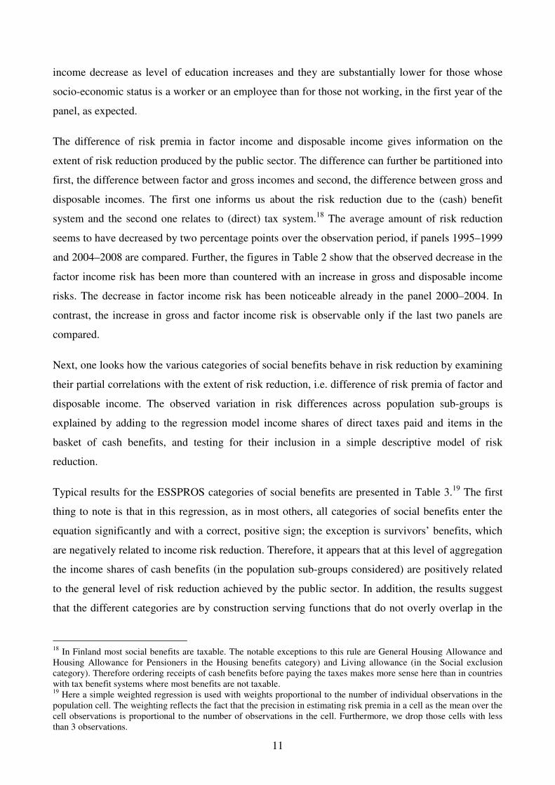
Next, one looks how the various categories of social benefits behave in risk reduction by examining

their partial correlations with the extent of risk reduction, i.e. difference of risk premia of factor and

disposable income. The observed variation in risk differences across population sub-groups is

explained by adding to the regression model income shares of direct taxes paid and items in the

basket of cash benefits, and testing for their inclusion in a simple descriptive model of risk

reduction.

Typical results for the ESSPROS categories of social benefits are presented in Table 3.19 The first

thing to note is that in this regression, as in most others, all categories of social benefits enter the

equation significantly and with a correct, positive sign; the exception is survivors’ benefits, which

are negatively related to income risk reduction. Therefore, it appears that at this level of aggregation

the income shares of cash benefits (in the population sub-groups considered) are positively related

to the general level of risk reduction achieved by the public sector. In addition, the results suggest

that the different categories are by construction serving functions that do not overly overlap in the

18 In Finland most social benefits are taxable. The notable exceptions to this rule are General Housing Allowance and Housing Allowance for Pensioners in the Housing benefits category) and Living allowance (in the Social exclusion category). Therefore ordering receipts of cash benefits before paying the taxes makes more sense here than in countries with tax benefit systems where most benefits are not taxable. 19 Here a simple weighted regression is used with weights proportional to the number of individual observations in the population cell. The weighting reflects the fact that the precision in estimating risk premia in a cell as the mean over the cell observations is proportional to the number of observations in the cell. Furthermore, we drop those cells with less than 3 observations.

12

type of income risk, they cover for. If this would not be the case then some categories might well

lose their significance.

It may be somewhat surprising to find out that the category, survivors’ benefits, enters the equation

with a negative, but significant sign. One plausible explanation is that those in the working-age are

not the primary group targeted by these benefits and the positive effects of risk reduction are missed

here, after controlling for all other benefits. However, survivors’ benefits are not among major

benefits; their share in disposable income is only under one percent. In addition, they are received

by a small part of the population and it could well be that more generous survivors benefits are

received by those population groups with less risk in factor income.

Our simple regression includes as additional terms Student benefits and Health insurance.

Interestingly enough, the category, Student benefits enters with a correct sign. One would have

expected similar problems than with survivors’ benefits, since both categories have small average

shares in disposable income and accrue to somewhat special population groups with presumably

little factor income.

The variable, Taxes merits some further comments. It has the correct, risk reducing sign that one

would expect from a progressive tax system that operates as an economy-wide automatic stabilizer.

Interestingly, the significance of this variable has been lost in the period 2004–2008, simultaneously

as its share in disposable income has been radically reduced. A concurrent decrease in the

Reynolds-Smolensky progressivity of taxation measure has been found by decomposing the change

in measure by the after-tax and before-tax income ratios and concentration coefficients in all

income deciles in Finland (Riihelä, Sullström & Suoniemi 2008). The decrease has been affected

most by changes at the high end of the income distribution.20 Unfortunately a more detailed

breakdown of the variable Taxes into capital, municipal and state (the progressive component of the

tax system) taxes is not available in the data and the issue cannot be pursued further.

Table 3 shows the results where the variables controlling for level of education have been included

to show that the results are robust to their inclusion and results do not change, qualitatively.

20 The main factor that has driven up the top income shares in Finland since the mid 1990s is in an unprecedented increase in the share of capital income, and the 1993 tax reform is seen as one of the key factors responsible for this trend as top incomes have become more and more composed of dividend income (Riihelä et al. 2008). The 1993 Finnish tax reform, introducing the Nordic dual income tax model, created strong incentives to shift earned income to capital income for those in the highest marginal tax brackets (Pirttilä and Selin 2006). The dual income tax treats capital and earned income differently. In those income groups facing high marginal tax rates in earned income, capital income is taxed using much lower rate. A strong correlation between the level of before-tax income and share of capital income offers an explanation for the decrease in progressivity of taxation, if shifting from earned income to dividend income becomes more popular with higher income.

13

Controlling for socio-economic status does not affect the qualitative results regarding the significant

variables, either. However, if the controls for the age-groups are entered, some coefficients become

unstable. It may well be that some ESSPROS categories of social benefit functions are covering

such special income risks which are more closely related to person’s age rather than his socio-

economic status or education level.

The above analysis ignores the redistributive components of social insurance. Next one looks into

those and the redistribution of income risk within age-cohorts that is provided by public tax-and-

benefit system.

Risk adjusted measure of permanent income and age

It has long been argued that distributions with income cumulated over a longer time horizon give a

better picture of economic welfare and income inequality than distributions based on snapshot

income. The age profiles of five year averages in factor and disposable income are shown among

the working-age population in Figures 1 and 2, respectively. Generally, the age profiles stay relative

flat from the early-thirties until the age group 40–44 years of age. After that the age profile rises

more steeply in factor income until there is a decline in mid-fifties as people start to retire. Gradual,

voluntary postponement of retirement age is likely to lay behind the temporal narrowing of the

income gap between those in the age group, 50–54, and those in the group, 55–59 years old. As

expected, the age profiles in average disposable income are substantially flatter than the

corresponding profile of factor income.

Above the undesirable effects of income fluctuations over time have been neglected. 21 The shift of

assessment to multi-period inequality and economic welfare would mean that uncertainty about

incomes must be accounted for in the evaluation procedure. Faced with less than perfect capital

markets, risk-averse economic agents view rise in income fluctuations as an increase in income risk

which lowers economic well-being in comparison with a steady flow of income. The uncertainty

aspect of income mobility is a key dimension of economic welfare. A completely mobile society

would mean complete economic insecurity.

Therefore, emphasis is now shifted to examining incomes which will be controlled for the risk

premium due to income fluctuations. In the calculations, the average equivalent income of each

individual is adjusted with the value of corresponding risk premium applicable to the population

21 Previously, we have examined Finnish income mobility from a positive point of view by considering the potentially beneficial effects of mobility on equalization of longer term income inequality (Suoniemi & Rantala 2010).

14

sub-group (defined by age group, education level and socio-economic status) which the individual

belongs to.22 Figure 3 compares the age-profiles of five year average real disposable income with

the corresponding risk-adjusted, certainty equivalent income concept in panel 2000–2004. The

difference between age-profiles reflects the value of risk aversion parameter chosen, ,3=ρ and the

difference is in the average equal to 1,580 € (7.7 percent relative risk premium) in equivalised

household disposable income (in 2008 prices). This corresponds to the monetary value which the

average working age households would be willing to forgo from a certain income level, and still be

as well off as with the random income flow, they face. In these terms and with our assumptions in

Finland the average risk in disposable income is of a reasonable size, if one considers the

precautionary saving motives.

Next we compare the distributions of mean real income and with the corresponding risk-adjusted,

certainty equivalent income. One may expect that the values of the Gini coefficient are somewhat

higher in the case of risk-adjusted income variables, since they incorporate some of the original

variation in income, though most of the individual variation has been smoothed out in the

estimation of the risk premia over population sub-groups. But mathematically this does need not

hold, since the reference point of the Gini coefficient, the mean is also changed, as one may observe

in Figure 4. The values of the Gini coefficient of risk-adjusted, certainty equivalent disposable

household income do not change noticeably in the working-age population; they are only 0.2–0.3

percentage points (about 1 percent) higher than those of average equivalised disposable household

income. The difference is largest in the youngest and smallest in the oldest age-group.

As noted above, the risk premia in household factor income are considerably higher than in

disposable income (Figure 5). In the 2000–2004 income panel data, estimations gave an average

relative risk premium of 23.9 percent, equivalent to 5,580 € in equivalised household factor income,

with .3=ρ 23 In the working-age population, especially young adults and older age cohorts face

more risk relative to others, and the mean values of risk premia in factor income range from 2,970 €

(40–44) to 6,450 € (20–24 years old). There is substantial labour market risk in Finland, even after

allowing for self-insurance by adjusting individual supply of working hours and family labour

supply. The comparison of results for factor and disposable income clearly shows the (utility) scale

22 Each age-group is treated differently in an effort to separate income fluctuations corresponding to income risk from the life-cycle pattern in income. This also motivates using a relatively short time-spans, 5 years. 23 Results based on alternative values, ,5,,1 K=ρ are in a great majority of cases qualitatively similar to these and the

reader should consult Tables 4–5, in the Appendix. The figures for value 0=ρ correspond to risk neutral preferences

and no adjustment for risk and a conservative choice of ,ρ the coefficient of relative risk aversion, ,1=ρ would

correspond to the logarithmic utility function.

15

of income insurance by the redistribution programs consisting of social benefits and progressive

taxation, and factor income risk of this magnitude is beyond those households’ means which occupy

the most risk-prone and low-income groups.24

In the case of disposable income the Gini coefficients of risk-adjusted, certainty equivalent

household income were a little higher than those of mean disposable household income. In the case

of factor income their roles are reversed. In the Finnish working-age population the values of the

Gini coefficient of risk-adjusted, certainty equivalent factor income are 2–3.5 percentage points

(almost 10 percent) higher than those of mean factor income (Figure 6). This means that those with

lower factor income are at the same time exposed to more risk in factor income.

There has been no marked change in the shape of age-income profiles of the Gini coefficient,

though the profiles show a steady income growth in the observation period 1995–2008 (Figure 7).

The values of the Gini coefficient are generally highest in the income panel 1995–1999 (Figure 8).

Subsequently, there has been a (within age-group) decrease in factor income inequality during the

observation period. But in the 2000’s, there has been hardly any change, with the exception of those

in the group, 55–59 years old which is due to gradual postponement of retirement age. The observed

temporal change in income inequality is in line with the corresponding change in unadjusted factor

income. If the whole population is considered, the Gini coefficients of household equivalised factor

income are 43.2, 43.4 and 43.6 percent, in the 1995–1999, 2000–2004 and 2004–2008 panel data,

respectively, and stay remarkably constant in the sample period.

In contrast, there has been a substantial increase in the Gini coefficients of certainty equivalent

household disposable income over the sample period with most of the change taking place between

the 1995–1999 and 2000–2004 panels. The change has been more marked in the distributions of the

youngest (20–24) and oldest (55–59) age cohorts (Figure 9).

Redistribution of income risk and income

Figure 10 shows, how the mean burden of the public net transfers underlying the redistribution

programs is shared in the working age population. On the average, all age groups seem to be net

payers until the mid-fifties, and the burden in €’s paid has been increasing (Figure 10). Note, that

24 An early study by Shorrocks (1980) reported that comparison of family income with male earnings showed limited opportunities to self-insurance by family labour supply.

16

pensioners, which are not shown here, are the biggest gainers. This may explain, why net payments

made by the working-age groups have increased on the average during the observation period. 25

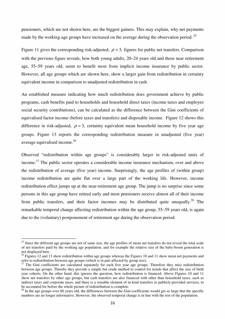
Figure 11 gives the corresponding risk-adjusted, ,3=ρ figures for public net transfers. Comparison

with the previous figure reveals, how both young adults, 20–24 years old and those near retirement

age, 55–59 years old, seem to benefit most from implicit income insurance by public sector.

However, all age groups which are shown here, show a larger gain from redistribution in certainty

equivalent income in comparison to unadjusted redistribution in cash.

An established measure indicating how much redistribution does government achieve by public

programs, cash benefits paid to households and household direct taxes (income taxes and employee

social security contributions), can be calculated as the difference between the Gini coefficients of

equivalised factor income (before taxes and transfers) and disposable income. Figure 12 shows this

difference in risk-adjusted, ,3=ρ certainty equivalent mean household income by five year age

groups. Figure 13 reports the corresponding redistribution measure in unadjusted (five year)

average equivalised income.26

Observed “redistribution within age groups” is considerably larger in risk-adjusted units of

income.27 The public sector operates a considerable income insurance mechanism, over and above

the redistribution of average (five year) income. Surprisingly, the age profiles of (within group)

income redistribution are quite flat over a large part of the working life. However, income

redistribution effect jumps up at the near-retirement age group. The jump is no surprise since some

persons in this age group have retired early and most pensioners receive almost all of their income

from public transfers, and their factor incomes may be distributed quite unequally.28 The

remarkable temporal change affecting redistribution within the age group, 55–59 years old, is again

due to the (voluntary) postponement of retirement age during the observation period.

25 Since the different age groups are not of same size, the age profiles of mean net transfers do not reveal the total scale of net transfers paid by the working age population, and for example the relative size of the baby-boom generation is not displayed here. 26 Figures 12 and 13 show redistribution within age groups whereas the Figures 10 and 11 show mean net payments and refer to redistribution between age groups (which is in part affected by group size). 27 The Gini coefficients are calculated separately for each five year age groups. Therefore they miss redistribution between age groups. Thereby they provide a simple but crude method to control for trends that affect the size of birth year cohorts. On the other hand, this ignores the question, how redistribution is financed. Above Figures 10 and 11 show net transfers by other age groups, but cash transfers are also financed with other than household taxes, such as indirect taxes and corporate taxes, and there is a sizeable element of in-kind transfers in publicly-provided services, to be accounted for before the whole picture of redistribution is complete. 28 In the age groups over 60 years old, the differences between the Gini-coefficients would get so large that the specific numbers are no longer informative. However, the observed temporal change is in line with the rest of the population.

17

More importantly, the data in average incomes point out that there has been a substantial cut-back

in public redistribution from the late 1990’s. For example, in the group, 35–39 old redistribution

effects, as measured by the difference of Gini coefficients, of risk-adjusted equivalised household

income were 16.9, 13,8 and 12,7 percentage points, in the 1995–1999, 2000–2004 and 2004–2008

income panel data, respectively (Table 6). In unadjusted equivalised household income the

corresponding figures were 14.1, 11.8 and 10.6. Differences of these numbers, taken here as

indicating redistribution of income risk, implicit income insurance by public sector, corresponds to

2–3 percentage points, or about 15–30 per cent of total amount of redistribution of equivalised

household income, using relative risk aversion coefficient, .3=ρ In the sample period

redistribution of both (five year) average unadjusted and risk-adjusted household income has

decreased by 3.5–4.0 percentage points (20–30 percent) if the 1995–1999 and 2004–2008 income

panel data are compared (Table 6).

Above we have shown results for a baseline choice of the relative risk aversion coefficient, ,3=ρ

as in Hoynes & Luttner (2011). Tables 4-6 give the results from calculations which vary the values

of ,ρ the coefficient of relative risk aversion. If a larger value is chosen, by definition the larger risk

premium one gets. In the 2000–2004 income panel data, with 1=ρ the average relative risk

premium is about 8.9 percent (2,860 €) in equivalised household factor income, with 5=ρ the risk

premium rises to 20.9 percent (6,750 €, Table 5). In terms of equivalised disposable income the

corresponding figures are 2.1 percent (600 €), 1=ρ , and 8.0 percent (2,250 €), 5=ρ (Table 4).

Similarly the extent of implicit public income insurance is increased with the value of ρ . For

example, in the 2000–2004 income panel data implicit income insurance, i.e. the difference between

the redistribution of risk-adjusted ( 1=ρ ) and unadjusted income ( 0=ρ ) is in the mean 1.8

percentage points, and it rises to 2.3 with 5=ρ (Table 6). If the change in the income redistribution

from the 1995–1999 income panel data to the 2004–2008 income panel data is considered, the

corresponding change increases slightly, with 1=ρ , the change (decrease) is 6.7 percentage points

with values gradually increasing up to 7.3, with .5=ρ If redistribution in mean income is

considered, figures with 0=ρ no risk, the average shows a 6.3 percentage points decrease.

In conclusion, income redistribution has been reduced in the sample period, and the result is not

dependent on whether one considers risk-adjusted income measures or cash measure. Above one

has found a decrease in factor income risk in the sample period. Although this may have reduced

18

the risk component in individual incomes the effect has not off-set the decrease in redistribution in

cash.

The changes observable in Figures 12 & 13 hold for redistribution effects within tightly defined age

groups (birth year cohorts), and do not tell the whole story about redistribution over the life-cycle.

This may explain, why net payments made by the working-age groups have increased on the

average during the observation period, although one found a decreased redistribution effect within

the age groups. The paper has considered changes in risk reduction and redistribution of risk in five

year age groups in the working age population. However, comparison of the adjacent age groups

across panels reveals changes in a five birth year cohorts over a 10 year time span, since, for

example those of 25–29 years old in the 1995–1999 income panel data will be 34–38 years old in

the 2004–2009 panel data.

5. DISCUSSION

Neoclassical welfare analysis which underlies most income distribution studies and public

economics is firmly anchored to static models under certainty. Income mobility is frequently seen to

represent a positive element in society whereas income risk imposes costs to risk-averse households

without access to perfect capital markets. How to introduce income mobility as an equalizer of

longer term income into the social objective function, while simultaneously recognising the role of

risk, is a demanding task (Fields 2010). The shift in assessment from annual to multi-period

inequality entails that future uncertainty about incomes must be accounted for in the evaluation.

This paper examined to what extent one can equate income mobility with income risk. Creedy et al.

(2011) present a framework which comes nearest to the one used in the current paper. Here relative

risk premia are estimated to adjust individual average incomes for risk aversion.

The paper looked at the inequality of longer term certainty equivalent (mean) incomes which have

been controlled for the undesirable effects of income fluctuations over time. In income mobility

studies the emphasis has been on the equalization of longer term inequality of mean income. To

obtain reasonable estimates of risk premia, level of education, socio-economic status and age,

factors likely to affect variability of income, are controlled for. A large number of observations

available in the data facilitates this rather detailed procedure based on weak distributional

assumptions. Naturally the results depend on the conditioning factors. Including more conditioning

factors one tends to get more variation in the estimators of income risk. In the extreme case one

19

would equate all income variation at the individual level with income risk. But all income variation

at the individual level is not to be equated with unpredictable income risk.29 The method used is a

simple and straight-forward one, and next step in the analysis would be to consider robustness of

results to the chosen set of conditioning factors used to estimate income risk.

In the current paper an effort has been made in separating income risk from the life-cycle effects on

the income process by conditioning the estimators of relative risk premium on age. This is an

important aspect and life-cycle effects should be given a more thoughtful treatment in studies of

income risk. In the future greater reliance on potentially volatile income sources in old age and

increasing longevity makes it more likely that older people may observe substantial changes in their

income.

The results look reasonable. The observed risk premia in household factor income were found to be

considerably higher than in disposable income. One found a decrease in factor income risk together

with an increase in gross and disposable income risks over the observation period 1995––2008. The

income shares of ESSPROS categories of social protection benefits in cash and direct taxes paid

entered the risk reduction (difference of risk premia of factor and disposable income) regression

equations with significant and correct, positive signs with the exception of survivors’ benefits.

Interestingly enough, additional terms, Student benefits and Health insurance also enter with a

correct sign. The results are robust to the inclusion of controls for education levels and for socio-

economic status. However, if the controls for the age-groups are entered, some coefficients become

unstable. It may well be that the ESSPROS categories of social benefit functions are covering such

income risks which are more closely related to person’s age.

The variable, direct taxes (income taxes and social security contributions) has the correct, risk

reducing sign that one would expect from a progressive tax system but the significance of this

variable has been lost in the period 2004–2008, simultaneously as its share in disposable income

has been radically reduced. This is in line with a previously found decrease in the Reynolds-

Smolensky progressivity of taxation measure (Riihelä, Sullström & Suoniemi 2008).

Therefore, it appears that at this level of aggregation the income shares of social benefits (in the

population sub-groups considered) are positively related to the general level of risk reduction

produced by the public sector. In addition, the results strongly suggest that the different categories

29 Creedy et al. (2011) estimate relative risk premia using three underlying parameters and relatively strong distributional assumptions, together with income in the initial period. The current paper utilises substantially more parameters (about 1000) to control for age, education level and socio-economic status in the initial period, together with mean income, and relatively weak distributional assumptions.

20

are by construction serving functions that do not overly overlap in the type of income risk, they

cover for. If this would not be the case then some categories might well lose their significance.

Remember that income risk reduction, i.e. reducing the variation of income, is considered here. A

positive function of social benefits in maintaining income would presumably be more

straightforward to find out.

Stiglitz and Youn (2005) have studied an ‘integrated lifetime insurance pension program’. Under

the integrated lifetime insurance pension an individual can use savings to provide cover for all

income risks, e.g. unemployment, health and disability. They show that so long as the risks are not

perfectly correlated then it pays to integrate all social insurance programs rather than to have

separate insurance programs covering each risk. The gain of joint integration-having a common

pool from which to draw upon—gets larger as the correlation gets smaller. The paper has presented

strong indirect evidence that the ESSPROSS system of social benefits cover for specific, separate

needs.

But note that the result holds for self-insurance. The possibility of pension-funded self-insurance

does not eliminate the desirability of some tax-funded insurance, except under extreme

circumstances (Stiglitz & Yun 2005). Additionally, I would like to remind that the Government

provides a common pool of resources and is the borrower/lender of last resort which offers huge

economies of scale and scope for any specific social benefit compared to what a pooling of separate

insurance accounts would provide at an individual level.

In the paper one compared the distributions of mean real income and with the corresponding risk-

adjusted, certainty equivalent income using the Gini coefficient. In the working-age population,

especially young adults and older age cohorts face more risk relative to others. There is substantial

labour market risk in Finland, even after allowing for self-insurance by adjusting individual supply

of working hours and family labour supply, and the results indicate the (utility) scale of income

insurance by the redistribution programs. In the case of disposable income the Gini coefficients of

certainty equivalent household income were little lower than those of mean disposable household

income. In the case of factor income their roles were reversed. In the Finnish working-age

population the values of the Gini coefficient of risk-adjusted, certainty equivalent factor income are

substantially higher than those of mean factor income which means that those with lower factor

income are at the same time exposed to more risk in factor income.

There has been hardly any change in risk-adjusted factor income inequality and the result holds also

for unadjusted factor income. In contrast, there has been a substantial increase in the Gini

21

coefficients of certainty equivalent household disposable income over the sample period with most

of the change taking place between the 1995–1999 and 2000–2004 panels. The change has been

more marked in the distributions of the youngest and oldest age cohorts.

Finally, the paper presented estimates on the redistribution effect using differences between Gini

coefficients of factor and disposable household income. Risk-adjusted¸ certainty equivalent income

concepts were used to get useful information on redistribution of risk, an additional indicator of

income insurance, and may be considered as adding to the literature. All age groups, including old

age people gain from redistribution in certainty equivalent income relative to unadjusted

redistribution of cash.

The corresponding Gini coefficients of certainty equivalent factor and disposable household income

depend on the degree of risk aversion assumed. However, the difference between these, an indicator

of redistribution of income risk, is influenced less by the degree of risk aversion assumed. In

addition, there has been a substantial cut-back in public redistribution in certainty equivalent

income and the finding is robust to a particular value of risk aversion parameter assumed.

Therefore, it is safe to conclude that the decrease in the mobility of disposable household income

observed in Rantala & Suoniemi (2010) which could have shown as lowered income risk has not

been large enough to off-set the effects of reduced redistribution in cash.

The paper considered certainty equivalent incomes which have been controlled for the undesirable

effects of income fluctuations over time. The reference point in risk premium calculations was

(observed) mean real income over the observation period. One can have several alternative choices

for the reference (status quo) point for risk measurement. The reference point may be based on

income in the first period, another reference may be based on a more sophisticated prediction of

future incomes (possibly with a deterministic or stochastic trend) than the simple average, which is

used in this paper. In a follow-up paper the present results are compared with those obtained by

substituting in the calculations for the forward looking estimators of the dynamic income process

(see, Creedy, Halvorsen & Thoresen 2013). In addition, income changes could be treated

asymmetrically, and one may give relatively more weight to losses than gains (see, prospect theory

by Kahneman & Tversky 1979). Furthermore, there is special merit in giving the risk of low-

income spells and poverty a special status in a thorough dynamic analysis.

In neoclassical theory the effects of public policies are taken into account by forward-looking,

rational economic agents while economic decisions on labour supply and savings are made. In

measuring the extent of risk reduction by the public tax-and-benefit system the paper has used

22

actual values observed during a particular episode in Finnish economy. Construction of the

counterfactual case of no public policies is a difficult problem, and the problem is frequently

ignored in analysing income distribution and income inequality. The current paper is no exception

to the rule. However, Hoynes & Luttner (2011) utilize matching across states to control for

differences in state tax-and-transfer policies and decompose the total value of state tax-and-transfer

programs into predictable changes in income and unexpected changes in income. The last effect is

used to obtain an estimate of the insurance value of state tax-and-transfer programs in the United

States. They find the total across person value of state tax-and-transfer programs as approximately

1,000 $ in 2005 dollars at the median real income, with 3=ρ . In the Finnish working age

population the risk-adjusted monetary equivalent of total redistribution is in the mean (controlling

for level of education, socio-economic status and age group) about 4,000 € larger in 2008 euros than

the corresponding redistribution in cash. In Finland the in-cash tax-and-transfer programs are more

extensive than the corresponding state programs in the United States (OECD, Social expenditure

database, SOCX). Furthermore, the methodology differs significantly.

Accounting for saving and borrowing decisions is outside the available data. To uncover joint

dynamics of income and consumption processes and to obtain more accurate measure of risk

premium would be desirable. However, such panel data sets are mostly unavailable and most of the

literature has resorted to using income data instead (Blundell & Etheridge 2010 is a notable

exception to the rule).

REFERENCES

Atkinson, A.B. (2000) The changing distribution of income: evidence and explanations, German

Economic Review, 1, 3–18.

Blundell, R. and B. Etheridge (2010) Consumption, income and earnings inequality in Britain, Review of Economics Dynamics, 13, 76–102.

Canberra group (2001) Expert Group on Household Income Statistics, Final Report and recommendations. Ottawa.

Carroll, C.D. (1994) How does future income affect current consumption? Quarterly Journal of

Economics, 109, 111–148.

Carroll, C.D. and Samwick, A.A. (1998) How important is precautionary saving? Review of

Economics and Statistics, 80, 410–419.

Creedy, J., and M. Wilhelm (2002) Income Mobility, Inequality and Social Welfare, Australian

Economic Papers, 41, 140–150.

Creedy, J., Halvorsen, E., and T. Thoresen (2013) Inequality comparisons in a multi-period framework: The role of alternative welfare metrics. Review of Income and Wealth, 59, 235-249.

23

Deaton, A. (1992) Understanding Consumption, Oxford: Oxford University Press.

Fields, G. S. (2008) Income Mobility. Articles & Chapters. Paper 453. http://digitalcommons.ilr.cornell.edu/articles/453.

Fields, G.S. (2010) Does Income Inequality Equalize Longer-term Incomes? New Measures of an Old Concept, Journal of Economic Inequality, 8, 409–427.

Fields, G. and Ok, E. (1999) The Measurement of Income Mobility: An Introduction to the Literature. In Handbook on Income Inequality Measurement, ed. J. Silber, Boston: Kluwer, 557–596.

Hoynes, H. and Luttmer, E. (2011) The insurance value of state tax-and-transfer programs. Journal

of Public Economics, 95, 1466–1484.

Jenkins, S. (2011) Changing Fortunes - Income Mobility and Poverty Dynamics in Britain. Oxford: Oxford University Press.

Kahneman, D., and Tversky, A. (1979) Prospect theory: An analysis of decision under risk. Econometrica, 47, 263-291.

Rantala J. and I. Suoniemi (2010) Income mobility, persistent inequality and age, recent experiences from Finland. Labour Institute for Economic Research, Working Papers, 263, http://www.labour.fi/tutkimusjulkaisut/tyopaperit/sel263.pdf.

Riihelä, M., Sullström R., & Suoniemi, I. (2008), Tax progressivity and recent evolution of the Finnish income inequality. Labour Institute for Economic Research, Working Papers, 246, http://www.labour.fi/tutkimusjulkaisut/tyopaperit/sel246.pdf.

Riihelä, M., Sullström, R. and Tuomala, M. (2007) Economic poverty in Finland, 1971–2004. Finnish Economic Papers, 21, 57–77.Shorrocks, A.F. (1978) Income inequality and income mobility, Journal of Economic Theory, 19, 376–393.

Riihelä, M., Sullström, R. & Tuomala, M. (2010), Trends in Top Income Shares in Finland 1966-2007, Tampere Economic Working Papers, Net Series no 78, University of Tampere.

Shorrocks, A.F. (1978) Income inequality and income mobility, Journal of Economic Theory, 19,

376-393.

Shorrocks, A.F. (1980) Income stability in the United States, Chapter 9 in Klevmarken, N.A. and Lybeck, J.A. (eds.) The Statics and Dynamics of Income. Oxford: Tieto Ltd.

Stiglitz, J. and J. Youn (2002) Integration of Unemployment Insurance with Retirement Insurance, NBER Working paper 9199.

Statistics Finland, Income Distribution Statistics, http://www.stat.fi/til/tjt/index_en.html.

24

Table 2. Descriptive statistics.

1995-99 2000-04 2004-08 Mean Std. Dev Mean Std. Dev Mean Std. Dev

Risk premium in Factor income 0.2211 0.1453 0.2069 0.1369 0.2098 0.1514 Risk premium in Gross income 0.0779 0.0557 0.0785 0.0491 0.0832 0.0624 Risk premium in Disposable income 0.0660 0.0487 0.0687 0.0433 0.0727 0.0574 Difference in risk premium Factor-Dispos. 0.1551 0.1260 0.1382 0.1208 0.1371 0.1287 Difference in risk premium Factor-Gross 0.1431 0.1228 0.1284 0.1185 0.1267 0.1266 Difference in risk premium Gross-Dispos. 0.0120 0.0101 0.0098 0.0084 0.0104 0.0077 Sickness/Health care 0.0059 0.0054 0.0062 0.0057 0.0068 0.0061 Disability 0.0571 0.1160 0.0487 0.1058 0.0473 0.1090 Old age 0.0480 0.0748 0.0402 0.0619 0.0338 0.0477 Survivors 0.0086 0.0141 0.0070 0.0128 0.0053 0.0084 Family/children 0.0517 0.0423 0.0392 0.0303 0.0373 0.0284 Unemployment 0.0659 0.0737 0.0495 0.0676 0.0456 0.0632 Housing 0.0103 0.0136 0.0106 0.0155 0.0109 0.0175 Social exclusion 0.0069 0.0118 0.0061 0.0120 0.0060 0.0137 Student 0.0080 0.0091 0.0056 0.0078 0.0045 0.0071 Health insurance 0.0159 0.0127 0.0148 0.0108 0.0162 0.0116 Taxes 0.4292 0.0883 0.3838 0.0773 0.3518 0.0748 Obs. in cells 303.557 544.378 350.853 588.781 357.897 587.628 Number of cells 862 754 745 Number of observations 261 666 264 543 266 633

Notes: Risk premia are calculated with the coefficient of relative risk aversion, 3=ρ . Benefits measured as share in

mean disposable equivalent income.

Table 3. Estimation results from a weighted regression for difference in risk premium.

Premium difference 1995-1999 2004-2008 Coefficient Std. Err. Coefficient Std. Err.

Sickness/Health care 1.3357*** 0.4135 1.9010*** 0.3714 Disability 0.3176*** 0.0164 0.3708*** 0.0206 Old age 0.8348*** 0.0384 0.8623*** 0.0428 Survivors -0.5151** 0.2497 -0.9372*** 0.2626 Family/children 0.2798*** 0.0713 0.6708*** 0.0918 Unemployment 0.6489*** 0.0164 0.8465*** 0.0193 Housing 1.3025*** 0.2620 0.8677*** 0.2103 Social exclusion 2.5615*** 0.2121 1.7808*** 0.1937 Student 2.3641*** 0.1604 2.8422*** 0.1748 Health insurance 1.5635*** 0.1952 0.5645*** 0.1839 Taxes 0.0791** 0.0368 0.0307 0.0419 Upper secondary level 0.0075 0.0032 0.0023 0.0030 Post-secondary before 2000 0.0091 0.0041 Lowest level tertiary 0.0030 0.0058 0.0022 0.0041 Lower-degree level tertiary 0.0053 0.0079 0.0069 0.0052 Higher-degree level tertiary -0.0026 0.0072 0.0018 0.0063 Doctorate level tertiary -0.0081 0.0179 0.0015 0.0139 constant -0.07594 0.02034 -0.04177 0.01815 R-squared 0.9475 0.9581 root MSE 0.0336 0.0276 Cells 862 745 Sum of weights (Obs.) 261 666 266 630 Notes: Dependent variable: Difference between risk premium in factor and disposable income, calculated with the

coefficient of relative risk aversion, 3=ρ , weighted regression with (cell) weights equal to the number of

observations in the cell. *** p<0.001, ** p<0.01, * p<0.05. * denotes significance at the 5 per cent level.

25

Figure 1. Average (five year) equivalised household factor income and age in 1995–1999, 2000–2004 and 2004–2008.

Figure 2. Average (five year) equivalised household disposable income and age in 1995–1999, 2000–2004 and 2004–2008.

6 000

10 000

14 000

18 000

22 000

26 000

30 000

20-24 25-29 30-34 35-39 40-44 45-49 50-54 55-59

1995 2000 2004

6 000

10 000

14 000

18 000

22 000

26 000

30 000

20-24 25-29 30-34 35-39 40-44 45-49 50-54 55-59

1995 2000 2004

26

Figure 3. Average (five year) equivalised household disposable income and risk-adjusted disposable income, ,3=ρ and age in 2000–2004.

10 000

14 000

18 000

22 000

26 000

20-24 25-29 30-34 35-39 40-44 45-49 50-54 55-59

Mean income Risk-adjusted mean income

Figure 4. The Gini coefficients of average equivalised household disposable income and risk-adjusted income ,3=ρ and age in 2000–2004.

0.16

0.18

0.20

0.22

0.24

0.26

20-24 25-29 30-34 35-39 40-44 45-49 50-54 55-59

Gini in mean income Gini in risk-adjusted

27

Figure 5. Average (five year) equivalised household factor income and risk-adjusted factor income, ,3=ρ and age in 2000–2004.

8 000

12 000

16 000

20 000

24 000

28 000

32 000

20-24 25-29 30-34 35-39 40-44 45-49 50-54 55-59

Mean income Risk-adjusted income

Figure 6. The Gini coefficients of average equivalised household factor income and risk-adjusted income ,3=ρ and age in 2000–2004.

0.28

0.36

0.44

0.52

0.6

20-24 25-29 30-34 35-39 40-44 45-49 50-54 55-59

Gini in mean income Gini in risk-adjusted mean income

28

Figure 7. Average (five year) risk-adjusted ,3=ρ equivalised household factor income and age in

1995–1999, 2000–2004 and 2004–2008.

6 000

10 000

14 000

18 000

22 000

26 000

30 000

20-24 25-29 30-34 35-39 40-44 45-49 50-54 55-59

1995 2000 2004

Figure 8. The Gini coefficient of average, risk-adjusted ,3=ρ equivalised household factor income

and age in 1995–1999, 2000–2004 and 2004–2008.

0.28

0.36

0.44

0.52

0.60

20-24 25-29 30-34 35-39 40-44 45-49 50-54 55-59

1995 2000 2004

29

Figure 9. The Gini coefficient of average, risk-adjusted ,3=ρ equivalised household disposable

income and age in 1995–1999, 2000–2004 and 2004–2008.

0.16

0.18

0.2

0.22

0.24

0.26

20-24 25-29 30-34 35-39 40-44 45-49 50-54 55-59

1995 2000 2004

Figure 10. Mean net transfers in average, equivalised household income and age in 1995–1999, 2000–2004 and 2004–2008.

-6 000

-3 000

0

3 000

6 000

9 000

20-24 25-29 30-34 35-39 40-44 45-49 50-54 55-59

1995 2000 2004

30

Figure 11. Mean net transfers in average, risk-adjusted ,3=ρ equivalised household income and

age in 1995–1999, 2000–2004 and 2004–2008.

-6 000

-3 000

0

3 000

6 000

9 000

20-24 25-29 30-34 35-39 40-44 45-49 50-54 55-59

1995 2000 2004

Figure 12. Public sector redistribution of average, equivalised household income and age in 1995–1999, 2000–2004 and 2004–2008.

0.08

0.16

0.24

0.32

0.40

20-24 25-29 30-34 35-39 40-44 45-49 50-54 55-59

1995 2000 2004

31

Figure 13. Public sector redistribution of average, risk-adjusted ,3=ρ equivalised household

income and age in 1995–1999, 2000–2004 and 2004–2008.

0.08

0.16

0.24

0.32

0.40

20-24 25-29 30-34 35-39 40-44 45-49 50-54 55-59

1995 2000 2004

32

APPENDIX

Below the estimators of relative risk premium are reported for real equivalised disposable

household income in the 2000–2004 income panel data with ,3=ρ by age and education level (6

levels) and socio-economic status (18 classes). Estimators are based on the means of the individual

risk premia in the population stratum in question.

The classifications in Tables A1 & A2 are coded as follows

Socio-economic status Code

farmer 10 self-employed 21 upper white collar employees - management 31 - research and planning 32 - education and teaching 33 - other 34 lower white collar employees - supervising 41 - independent work 42 - non-independent work 43 - other 44 blue collar workers - agricultural 51 - industrial 52 - other production 53 - service and logistics 54 students 60 pensioners 70 long-term unemployed 81 others not elsewhere classified or status unknown 99 Education level Code

primary & lower secondary or unknown 2 upper & post secondary 3 Lowest level tertiary 5 Bachelor or equivalent 6 Masters or equivalent 7 Doctorate or equivalent 8

33

Table 4. Average risk-adjusted household disposable income in the five-year income panel data, in 1995–1999, 2000–2004 and 2004–2008. Age Panel

ρ 20–24 25–29 30–34 35–39 40–44 45–49 50–54 55–59

1995–1999 0 16076 17527 17917 17879 18216 19424 20253 18388 1 15436 17103 17595 17595 17922 19078 19912 18107 2 14838 16710 17302 17338 17655 18772 19614 17867 3 14347 16384 17063 17127 17435 18524 19374 17672 4 13956 16112 16861 16948 17247 18314 19170 17507 5 13645 15884 16688 16796 17086 18135 18996 17366 2000–2004 0 18123 20595 20841 20572 20842 22108 23085 22277 1 17322 20055 20430 20216 20487 21726 22677 21918 2 16583 19557 20062 19901 20172 21388 22325 21612 3 15991 19146 19762 19644 19912 21110 22041 21366 4 15525 18806 19508 19426 19692 20874 21802 21160 5 15159 18522 19292 19240 19505 20670 21598 20983 2004–2008 0 19453 22758 23679 23484 23423 24691 25585 24971 1 18512 22117 23198 23051 23006 24236 25132 24546 2 17659 21530 22768 22672 22643 23846 24750 24194 3 16987 21058 22417 22370 22349 23535 24447 23912 4 16466 20672 22123 22118 22102 23272 24193 23675 5 16059 20353 21873 21905 21892 23047 23977 23474

Table 5. Average risk-adjusted household factor income in the five-year income panel data, in 1995–1999, 2000–2004 and 2004–2008.

Age

Panel ρ 20–24 25–29 30–34 35–39 40–44 45–49 50–54 55–59

1995–1999 0 17328 19763 20504 21012 21955 23607 22999 14467

1 14073 17483 18775 19548 20549 22051 20886 11559

2 11939 15928 17591 18564 19631 21063 19711 10253

3 10961 15105 16922 18008 19112 20512 19128 9750

4 10370 14546 16446 17607 18735 20111 18723 9444

5 9970 14136 16080 17298 18440 19797 18414 9229

2000–2004 0 20197 24484 24690 24516 25266 26888 26857 20598

1 16970 22253 22900 22957 23797 25301 24755 17374

2 14825 20700 21697 21935 22850 24309 23557 15864

3 13745 19792 20981 21340 22295 23739 22924 15217

4 13064 19143 20450 20902 21886 23315 22473 14803

5 12591 18653 20035 20558 21564 22979 22125 14505

2004–2008 0 21297 26715 28065 28057 28229 29881 30031 24827

1 17802 24286 26093 26305 26578 28126 27997 21458

2 15547 22631 24774 25178 25562 27068 26823 19862

3 14412 21657 23967 24501 24961 26442 26163 19131

4 13692 20961 23360 23996 24512 25970 25682 18648

5 13192 20432 22882 23598 24156 25593 25306 18294

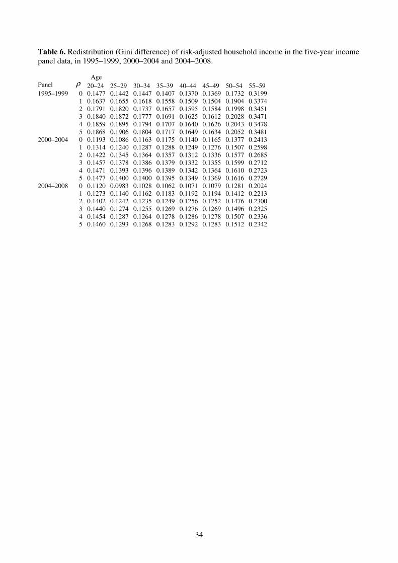
34

Table 6. Redistribution (Gini difference) of risk-adjusted household income in the five-year income panel data, in 1995–1999, 2000–2004 and 2004–2008. Age Panel ρ 20–24 25–29 30–34 35–39 40–44 45–49 50–54 55–59 1995–1999 0 0.1477 0.1442 0.1447 0.1407 0.1370 0.1369 0.1732 0.3199 1 0.1637 0.1655 0.1618 0.1558 0.1509 0.1504 0.1904 0.3374 2 0.1791 0.1820 0.1737 0.1657 0.1595 0.1584 0.1998 0.3451 3 0.1840 0.1872 0.1777 0.1691 0.1625 0.1612 0.2028 0.3471 4 0.1859 0.1895 0.1794 0.1707 0.1640 0.1626 0.2043 0.3478 5 0.1868 0.1906 0.1804 0.1717 0.1649 0.1634 0.2052 0.3481 2000–2004 0 0.1193 0.1086 0.1163 0.1175 0.1140 0.1165 0.1377 0.2413 1 0.1314 0.1240 0.1287 0.1288 0.1249 0.1276 0.1507 0.2598 2 0.1422 0.1345 0.1364 0.1357 0.1312 0.1336 0.1577 0.2685 3 0.1457 0.1378 0.1386 0.1379 0.1332 0.1355 0.1599 0.2712 4 0.1471 0.1393 0.1396 0.1389 0.1342 0.1364 0.1610 0.2723 5 0.1477 0.1400 0.1400 0.1395 0.1349 0.1369 0.1616 0.2729 2004–2008 0 0.1120 0.0983 0.1028 0.1062 0.1071 0.1079 0.1281 0.2024 1 0.1273 0.1140 0.1162 0.1183 0.1192 0.1194 0.1412 0.2213 2 0.1402 0.1242 0.1235 0.1249 0.1256 0.1252 0.1476 0.2300 3 0.1440 0.1274 0.1255 0.1269 0.1276 0.1269 0.1496 0.2325 4 0.1454 0.1287 0.1264 0.1278 0.1286 0.1278 0.1507 0.2336 5 0.1460 0.1293 0.1268 0.1283 0.1292 0.1283 0.1512 0.2342

35

Table A1. Relative risk premium in factor income in the 2000–2004 panel data with ,3=ρ by age,

education level (6 levels) and socio-economic status (18 classes) in 2004.

Socio-econ. Status

Education level

20–24

25–29

30–34

35–39

40–44

45–49

50–54

55–59

10 2 0.3538 0.3622 0.2218 0.1977 0.1830 0.1973 0.2079 0.2535 10 3 0.2244 0.2507 0.2262 0.1792 0.1818 0.1686 0.1974 0.2329 10 5 . 0.2165 0.1539 0.1594 0.1866 0.1934 0.1795 0.2498 10 6 0.3917 0.1699 0.1639 0.1193 0.1508 0.1244 0.1335 0.1946 10 7 . 0.1409 0.2342 0.2719 0.1221 0.3198 0.1554 0.2600 10 8 . . 0.1156 . 0.6286 . . . 21 2 0.3967 0.3217 0.3119 0.2481 0.2223 0.2066 0.2035 0.2245 21 3 0.3319 0.2580 0.2289 0.2126 0.1729 0.1890 0.1869 0.2157 21 5 . 0.1933 0.2080 0.1830 0.1696 0.1419 0.1824 0.1930 21 6 0.2943 0.2849 0.2260 0.1581 0.1994 0.1815 0.1886 0.1800 21 7 . 0.1256 0.2058 0.1799 0.1346 0.1484 0.1267 0.1525 21 8 . . 0.5584 0.0474 0.0545 0.1242 0.1375 0.0777 31 2 0.6127 0.1120 0.0963 0.1574 0.1445 0.1797 0.1359 0.1566 31 3 0.2918 0.1206 0.1046 0.1239 0.0978 0.0813 0.0834 0.1652 31 5 0.2672 0.0957 0.1188 0.0860 0.0809 0.0650 0.0756 0.1123 31 6 0.0977 0.0903 0.0916 0.0526 0.0461 0.0655 0.0584 0.1294 31 7 0.0723 0.0802 0.0779 0.0657 0.0429 0.0428 0.0702 0.0808 31 8 . 0.2079 0.0588 0.0234 0.0276 0.0438 0.0497 0.0694 32 2 0.3346 0.2217 0.1620 0.1548 0.1301 0.0711 0.0863 0.1808 32 3 0.2394 0.1422 0.0863 0.0861 0.0660 0.0727 0.0495 0.1671 32 5 . 0.1122 0.0725 0.0740 0.0684 0.0562 0.0451 0.1565 32 6 0.1621 0.0858 0.0769 0.0641 0.0577 0.0585 0.0655 0.1021 32 7 0.1890 0.1179 0.0973 0.0765 0.0638 0.0714 0.0492 0.0890 32 8 . 0.1535 0.0836 0.0760 0.0870 0.0983 0.0382 0.0744 33 2 0.2546 0.2935 0.2111 0.1873 0.1389 0.0801 0.1932 0.2650 33 3 0.3223 0.1976 0.1671 0.1493 0.1010 0.0894 0.1222 0.1997 33 5 . 0.1438 0.1224 0.1076 0.0765 0.0832 0.0780 0.1438 33 6 0.2664 0.1526 0.1180 0.0810 0.0725 0.0668 0.0758 0.2747 33 7 0.1219 0.1087 0.0921 0.0708 0.0509 0.0578 0.0749 0.1367 33 8 0.0836 0.1388 0.0887 0.0711 0.0779 0.0547 0.0689 0.1374 34 2 0.3056 0.1732 0.2102 0.1404 0.1224 0.0826 0.0930 0.1795 34 3 0.3123 0.1891 0.1135 0.0964 0.1144 0.0676 0.0858 0.1700 34 5 . 0.1094 0.1255 0.0769 0.0567 0.0727 0.0790 0.2100 34 6 0.2596 0.1257 0.1170 0.0762 0.0488 0.0515 0.0813 0.1532 34 7 0.0945 0.1203 0.1018 0.0808 0.0688 0.0596 0.0603 0.0977 34 8 . 0.1110 0.1094 0.1525 0.0837 0.0866 0.0331 0.0596 41 2 0.3140 0.1244 0.1646 0.1052 0.1148 0.0827 0.0799 0.2351 41 3 0.2363 0.1351 0.0949 0.0771 0.0698 0.0914 0.0807 0.1905 41 5 0.0630 0.1229 0.0771 0.0591 0.0620 0.0621 0.0538 0.1462 41 6 0.1414 0.0787 0.0582 0.0487 0.0431 0.0599 0.0556 0.0852 41 7 0.0599 0.0838 0.0697 0.0603 0.0410 0.0453 0.0484 0.1614 41 8 . 0.2039 0.0757 0.0315 0.0151 0.0282 0.0052 0.0011 42 2 0.2878 0.1966 0.1479 0.1501 0.0929 0.0955 0.1006 0.2067 42 3 0.2373 0.1563 0.1228 0.1021 0.0880 0.0879 0.0886 0.2044 42 5 0.5983 0.1259 0.0998 0.0784 0.0700 0.0695 0.0822 0.1411 42 6 0.1364 0.1099 0.0991 0.0771 0.0644 0.0511 0.0798 0.1080 42 7 0.2539 0.1310 0.0972 0.0884 0.0797 0.0796 0.0524 0.1214 42 8 . . 0.0972 0.0751 0.0442 0.1026 0.0389 0.0605 43 2 0.3105 0.2553 0.1897 0.1520 0.1292 0.0982 0.1100 0.2301 43 3 0.2887 0.2298 0.1805 0.1254 0.0988 0.1072 0.1093 0.2201 43 5 0.1661 0.1274 0.1155 0.0996 0.0763 0.0980 0.1042 0.2031 43 6 0.1436 0.1640 0.1212 0.0997 0.0542 0.0731 0.0318 0.0481 43 7 0.1017 0.1539 0.1609 0.0744 0.1327 0.0945 0.5810 0.1725 43 8 . . 0.2454 0.0590 . 0.0839 . . 44 2 0.3565 0.2410 0.2039 0.1798 0.1460 0.1088 0.1307 0.2357 44 3 0.2261 0.1506 0.1278 0.0986 0.0815 0.0862 0.0936 0.2249

36

44 5 0.2521 0.1202 0.1026 0.0788 0.0591 0.0685 0.0825 0.2087 44 6 0.1368 0.1075 0.1110 0.0904 0.0789 0.0679 0.0996 0.1344 44 7 0.2320 0.1969 0.1556 0.0686 0.0610 0.1212 0.0893 0.1064 44 8 . . 0.7715 0.1941 0.2412 0.0461 0.0881 . 51 2 0.2422 0.2328 0.1683 0.1558 0.1181 0.1129 0.1475 0.2544 51 3 0.1914 0.1426 0.1300 0.1386 0.1187 0.1085 0.1329 0.2310 51 5 . 0.0894 0.1935 0.1187 0.1249 0.1412 0.2307 0.1175 51 6 0.1276 0.1381 0.2102 0.1067 0.0272 0.3501 0.0380 0.6226 51 7 . 0.3742 0.1837 0.1546 . 0.4373 0.2012 . 51 8 . . . . . 0.0246 . . 52 2 0.2287 0.1699 0.1388 0.1259 0.1145 0.0850 0.1164 0.2546 52 3 0.1682 0.1190 0.1020 0.0848 0.0869 0.0824 0.0993 0.2109 52 5 0.0228 0.1295 0.0857 0.0816 0.0803 0.0878 0.1096 0.1847 52 6 0.2325 0.1212 0.1089 0.0651 0.1429 0.0888 0.2017 0.1432 52 7 0.3355 0.1442 0.1588 0.1431 0.0957 0.1511 0.1858 0.5113 52 8 . . 0.5900 0.1662 . . 0.0284 . 53 2 0.2620 0.2111 0.2016 0.1412 0.1374 0.1094 0.1150 0.2229 53 3 0.2230 0.1554 0.1137 0.1012 0.0908 0.0947 0.1119 0.2216 53 5 0.1187 0.1141 0.0936 0.1045 0.0867 0.1097 0.1221 0.1480 53 6 0.1967 0.1545 0.0821 0.1038 0.0707 0.0142 0.0473 0.1869 53 7 0.2785 0.0984 0.2027 0.1982 0.0111 0.3431 0.1852 . 53 8 . . 0.1458 . . . . . 54 2 0.2787 0.2436 0.1758 0.1522 0.1401 0.1325 0.1240 0.2270 54 3 0.2413 0.1699 0.1386 0.1222 0.1038 0.1089 0.1304 0.2261 54 5 0.2060 0.1378 0.1194 0.1258 0.1195 0.1533 0.1217 0.2052 54 6 0.2074 0.1491 0.1424 0.1210 0.1934 0.2286 0.1386 0.1545 54 7 0.6517 0.1264 0.2743 0.1769 0.1821 0.0953 0.1620 0.4060 54 8 . . . 0.2237 . . 0.0841 0.0111 60 2 0.6146 0.5838 0.5706 0.5250 0.5914 0.5397 0.4909 0.5827 60 3 0.4476 0.4615 0.4741 0.4925 0.4932 0.4187 0.4690 0.4373 60 5 0.6385 0.4198 0.3932 0.3851 0.3907 0.4705 0.3903 0.6418 60 6 0.3303 0.3987 0.3368 0.3654 0.5472 0.3779 0.4144 0.5324 60 7 0.3177 0.3663 0.3267 0.3749 0.3949 0.4338 0.2774 0.5752 60 8 . 0.4465 0.4627 0.3291 0.4700 0.5681 0.1098 0.3191 70 2 0.4298 0.4344 0.3908 0.3937 0.3787 0.3939 0.3864 0.4252 70 3 0.5283 0.4297 0.4439 0.4473 0.3894 0.3900 0.3975 0.4265 70 5 . 0.4428 0.4853 0.4680 0.4542 0.3828 0.3905 0.4156 70 6 0.4665 0.5893 0.6488 0.4353 0.5102 0.5143 0.4761 0.3858 70 7 . 0.5065 0.5091 0.5475 0.4173 0.4589 0.3292 0.4116 70 8 . . . . 0.3070 0.8472 0.2642 0.4202 81 2 0.6239 0.5786 0.5576 0.5519 0.5306 0.4795 0.4560 0.5259 81 3 0.4806 0.4606 0.4520 0.4402 0.4602 0.4432 0.4316 0.4950 81 5 0.4594 0.3488 0.3367 0.4049 0.3996 0.4383 0.4523 0.4710 81 6 0.3770 0.3922 0.3819 0.3751 0.4627 0.4001 0.4142 0.4255 81 7 0.3485 0.3710 0.4325 0.3646 0.4837 0.4325 0.4687 0.5694 81 8 . 0.1139 0.5212 0.3020 0.4984 0.3751 0.1194 0.2380 99 2 0.5441 0.6101 0.5755 0.5604 0.5077 0.4365 0.4510 0.4639 99 3 0.4180 0.4413 0.4757 0.4953 0.4335 0.4468 0.4377 0.4580 99 5 0.5367 0.4704 0.4777 0.4130 0.4763 0.4201 0.3413 0.3461 99 6 0.3228 0.3129 0.3076 0.4561 0.3610 0.3516 0.3942 0.5058 99 7 0.5034 0.3828 0.3740 0.3807 0.3460 0.5188 0.5696 0.4226 99 8 . . . 0.5371 0.6571 0.1431 0.3715 0.9111

37

Table A2. Relative risk premium in disposable in the 2000–2004 panel data with ,3=ρ by age,

education level (6 levels) and socio-economic status (18 classes) in 2004.

Socio-econ. Status

Education level

Age 2004 20–24

25–29

30–34

35–39

40–44

45–49

50–54

55–59

10 2 0.1588 0.1968 0.1274 0.1062 0.0883 0.1165 0.1253 0.1406

10 3 0.1224 0.1363 0.1140 0.0936 0.1079 0.1097 0.1211 0.1225

10 5 . 0.1062 0.0890 0.0936 0.1203 0.1211 0.1290 0.1198

10 6 0.2574 0.0927 0.0648 0.0975 0.1154 0.0975 0.1031 0.1070

10 7 . 0.0549 0.2027 0.1248 0.0952 0.2321 0.0951 0.1302

10 8 . . 0.0255 . 0.1727 . . .

21 2 0.1993 0.1644 0.1910 0.1320 0.1186 0.1314 0.1214 0.1084

21 3 0.1918 0.1452 0.1085 0.1192 0.0981 0.1125 0.1098 0.1031

21 5 . 0.1073 0.1092 0.1024 0.0984 0.0926 0.1233 0.1032

21 6 0.1672 0.1614 0.1240 0.0758 0.1191 0.1111 0.1304 0.1050

21 7 . 0.0760 0.1119 0.1012 0.0705 0.1075 0.0793 0.1000

21 8 . . 0.2595 0.0117 0.0602 0.0769 0.0616 0.0707

31 2 0.3985 0.0713 0.0510 0.0957 0.0754 0.0911 0.0651 0.0389

31 3 0.1674 0.0758 0.0496 0.0535 0.0504 0.0404 0.0355 0.0468

31 5 0.2055 0.0720 0.0548 0.0544 0.0475 0.0380 0.0411 0.0277

31 6 0.0743 0.0451 0.0398 0.0276 0.0309 0.0393 0.0335 0.0245

31 7 0.0542 0.0529 0.0412 0.0411 0.0297 0.0280 0.0342 0.0235

31 8 . 0.1278 0.0399 0.0136 0.0227 0.0406 0.0333 0.0277

32 2 0.1482 0.1239 0.0792 0.0961 0.0619 0.0411 0.0299 0.0296

32 3 0.1107 0.0690 0.0433 0.0444 0.0271 0.0429 0.0327 0.0399

32 5 . 0.0440 0.0365 0.0333 0.0348 0.0276 0.0242 0.0325

32 6 0.0807 0.0437 0.0352 0.0326 0.0294 0.0307 0.0306 0.0237

32 7 0.1123 0.0685 0.0502 0.0416 0.0376 0.0393 0.0279 0.0256

32 8 . 0.0579 0.0422 0.0400 0.0442 0.0629 0.0253 0.0328

33 2 0.0968 0.0743 0.0655 0.0543 0.0927 0.0496 0.1035 0.0382

33 3 0.1509 0.0916 0.0647 0.0572 0.0360 0.0388 0.0476 0.0458

33 5 . 0.0567 0.0458 0.0434 0.0443 0.0433 0.0405 0.0345

33 6 0.1094 0.0631 0.0525 0.0349 0.0362 0.0388 0.0315 0.0323

33 7 0.0625 0.0563 0.0426 0.0343 0.0295 0.0332 0.0356 0.0315

33 8 0.0129 0.1051 0.0421 0.0362 0.0521 0.0380 0.0376 0.0443

34 2 0.1623 0.0891 0.0893 0.0601 0.0885 0.0569 0.0276 0.0357

34 3 0.1635 0.0928 0.0581 0.0517 0.0525 0.0306 0.0337 0.0309

34 5 . 0.0499 0.0579 0.0410 0.0312 0.0425 0.0410 0.0345

34 6 0.1157 0.0640 0.0590 0.0322 0.0251 0.0299 0.0352 0.0327

34 7 0.0566 0.0647 0.0493 0.0420 0.0395 0.0347 0.0331 0.0261

34 8 . 0.0829 0.0585 0.0701 0.0388 0.0506 0.0289 0.0295

41 2 0.1269 0.0490 0.0789 0.0303 0.0489 0.0387 0.0251 0.0321

41 3 0.1140 0.0614 0.0361 0.0318 0.0350 0.0370 0.0348 0.0283

41 5 0.0334 0.0512 0.0346 0.0262 0.0314 0.0302 0.0257 0.0262

41 6 0.0667 0.0379 0.0288 0.0221 0.0235 0.0395 0.0291 0.0211

41 7 0.0378 0.0509 0.0331 0.0309 0.0259 0.0289 0.0393 0.0492

41 8 . 0.1407 0.0315 0.0169 0.0126 0.0360 0.0049 0.0010

42 2 0.1071 0.0630 0.0496 0.0459 0.0400 0.0453 0.0349 0.0336

42 3 0.1089 0.0715 0.0447 0.0378 0.0386 0.0393 0.0353 0.0344

42 5 0.0827 0.0493 0.0450 0.0365 0.0371 0.0359 0.0343 0.0302

42 6 0.0770 0.0532 0.0430 0.0321 0.0295 0.0297 0.0426 0.0340

42 7 0.1742 0.0669 0.0460 0.0508 0.0441 0.0411 0.0376 0.0440

42 8 . . 0.0920 0.0153 0.0204 0.0543 0.0381 0.0519

43 2 0.1101 0.0649 0.0348 0.0460 0.0509 0.0420 0.0394 0.0469

43 3 0.1340 0.0985 0.0711 0.0390 0.0418 0.0415 0.0431 0.0411

43 5 0.1480 0.0565 0.0335 0.0317 0.0357 0.0456 0.0346 0.0427

43 6 0.0851 0.0787 0.0482 0.0441 0.0219 0.0411 0.0311 0.0281

38

43 7 0.0707 0.0964 0.0611 0.0298 0.0406 0.0314 0.0140 0.0797

43 8 . . 0.1695 0.0253 . 0.0735 . .

44 2 0.1313 0.0669 0.0519 0.0406 0.0430 0.0342 0.0296 0.0309

44 3 0.0979 0.0548 0.0394 0.0383 0.0350 0.0360 0.0302 0.0300

44 5 0.0927 0.0461 0.0388 0.0365 0.0338 0.0392 0.0355 0.0382

44 6 0.0617 0.0492 0.0438 0.0414 0.0390 0.0379 0.0408 0.0430

44 7 0.1281 0.0884 0.0704 0.0342 0.0223 0.0458 0.0673 0.0276

44 8 . . 0.5590 0.1680 0.1624 0.0204 0.0244 .

51 2 0.1038 0.0713 0.0454 0.0516 0.0431 0.0534 0.0366 0.0315

51 3 0.0931 0.0598 0.0429 0.0446 0.0410 0.0403 0.0508 0.0538

51 5 . 0.0433 0.0524 0.0505 0.0774 0.0358 0.1137 0.0793

51 6 0.0779 0.0794 0.1597 0.0386 0.0154 0.0373 0.0236 0.0622

51 7 . 0.2537 0.1269 0.1405 . 0.0681 0.1779 .

51 8 . . . . . 0.0036 . .

52 2 0.0835 0.0624 0.0400 0.0413 0.0374 0.0284 0.0267 0.0305

52 3 0.0731 0.0420 0.0326 0.0274 0.0279 0.0318 0.0262 0.0279

52 5 0.0155 0.0427 0.0313 0.0280 0.0351 0.0339 0.0315 0.0279

52 6 0.0870 0.0530 0.0321 0.0283 0.0317 0.0527 0.0859 0.0249

52 7 0.2166 0.0701 0.0378 0.0523 0.0324 0.0414 0.1016 0.0383

52 8 . . 0.0251 0.0684 . . 0.0243 .

53 2 0.0869 0.0574 0.0585 0.0440 0.0383 0.0317 0.0314 0.0342

53 3 0.0933 0.0545 0.0325 0.0305 0.0320 0.0306 0.0292 0.0273

53 5 0.0217 0.0403 0.0331 0.0332 0.0327 0.0465 0.0443 0.0256

53 6 0.1174 0.0589 0.0295 0.0286 0.0425 0.0116 0.0285 0.0398

53 7 0.0987 0.0745 0.1465 0.0423 0.0080 0.2606 0.1216 .

53 8 . . 0.0874 . . . . .

54 2 0.0902 0.0817 0.0429 0.0465 0.0444 0.0373 0.0285 0.0301

54 3 0.1011 0.0617 0.0418 0.0357 0.0365 0.0337 0.0323 0.0319

54 5 0.0833 0.0569 0.0482 0.0459 0.0433 0.0557 0.0328 0.0347

54 6 0.0904 0.0654 0.0705 0.0458 0.0451 0.0960 0.0490 0.0283

54 7 0.3320 0.0760 0.0989 0.0450 0.0640 0.0349 0.0795 0.0644

54 8 . . . 0.0145 . . 0.0626 0.0202

60 2 0.1643 0.1372 0.0905 0.0896 0.0647 0.0744 0.0736 0.0800

60 3 0.1748 0.1692 0.1175 0.0971 0.0858 0.0716 0.0848 0.0755

60 5 0.1086 0.1404 0.1243 0.0778 0.0716 0.0869 0.0702 0.0732

60 6 0.1484 0.1473 0.1294 0.1106 0.1343 0.0999 0.0955 0.1514

60 7 0.1440 0.1958 0.1351 0.1598 0.1020 0.1427 0.1167 0.0678

60 8 . 0.1831 0.3222 0.2733 0.2470 0.2729 0.0941 0.0295

70 2 0.0623 0.0565 0.0422 0.0358 0.0375 0.0338 0.0316 0.0333

70 3 0.1006 0.0638 0.0409 0.0454 0.0347 0.0389 0.0358 0.0334

70 5 . 0.0561 0.0570 0.0626 0.0500 0.0470 0.0401 0.0310

70 6 0.0822 0.1281 0.0991 0.0366 0.0555 0.0477 0.0421 0.0335

70 7 . 0.0654 0.0418 0.1421 0.0909 0.0815 0.0502 0.0315

70 8 . . . . 0.0146 0.0592 0.2193 0.1081

81 2 0.1192 0.0834 0.0685 0.0646 0.0649 0.0625 0.0553 0.0422

81 3 0.1191 0.0813 0.0711 0.0612 0.0603 0.0606 0.0606 0.0422

81 5 0.1111 0.0641 0.0655 0.0640 0.0610 0.0606 0.0623 0.0575

81 6 0.1360 0.1027 0.0736 0.0598 0.0773 0.0767 0.0847 0.0694

81 7 0.1066 0.1382 0.1199 0.1017 0.0858 0.0954 0.0839 0.0789

81 8 . 0.0785 0.1893 0.0529 0.1643 0.0487 0.0522 0.0310

99 2 0.1594 0.1546 0.1466 0.1392 0.1441 0.1595 0.1330 0.1435

99 3 0.1665 0.1416 0.1178 0.1308 0.1216 0.1370 0.1253 0.1206

99 5 0.1298 0.1179 0.1376 0.1006 0.1796 0.1835 0.1837 0.1840

99 6 0.1626 0.1119 0.1004 0.1517 0.1103 0.2014 0.1716 0.3463

99 7 0.3737 0.1434 0.1891 0.1926 0.1239 0.2677 0.3077 0.2079

99 8 . . . 0.4602 0.6503 0.0048 0.3560 0.1939