permittivity

Devendra K. Misra. "Permittivity Measurement."

Copyright 2000 CRC Press LLC. <http://www.engnetbase.com>.

PermittivityMeasurement

46.1 Measurement of Complex Permittivity at Low Frequencies

46.2 Measurement of Complex Permittivity Using Distributed CircuitsResonant Cavity Method • Free-Space Method for Measurement of Complex Permittivity • A Nondestructive Method for Measuring the Complex Permittivity of Materials

Dielectric materials possess relatively few free charge carriers. Most of the charge carriers are bound andcannot participate in conduction. However, these bound charges can be displaced by applying an externalelectric field. In such cases, the atom or molecule forms an electric dipole that maintains an electric field.Consequently, each volume element of the material behaves as an electric dipole. The dipole field tendsto oppose the applied field. Dielectric materials that exhibit nonzero distribution of such bound chargeseparations are said to be polarized. The volume density of polarization

→P describes the volume density

of those electric dipoles. When a material is linear and isotropic in nature, the polarization density isrelated to applied electric field intensity,

→E, as follows:

(46.1)

where ε0 (= 8.854 × 10–12 F m–1) is the permittivity of free-space and χe is called the electric susceptibilityof the material.

The electric flux density, or displacement,→D is defined as follows:

(46.2)

where ε is called the permittivity of the material and εr is its relative permittivity or dielectric constant.Electric flux density is expressed in coulombs per meter (C m–1).

Equation 46.2 represents a relation between the electric flux density and electric field intensity infrequency domain. It will hold well in time-domain only if the permittivity is independent of frequency.A material is called dispersive if its characteristics are frequency dependent. The product of Equation 46.2in frequency domain will be replaced by a convolution integral for the time-domain fields.

Assuming that the fields are time-harmonic as e jωt, the generalized Ampere’s law can be expressed inphasor form as follows:

(46.3)

r rP E= ε χ0 e

r r r r r rD E P E E E= + = +( ) = =ε ε χ ε ε ε0 0 01 o r

∇ × = + +r r r r

H J J j De ω

Devendra K. MisraUniversity of Wisconsin

© 1999 by CRC Press LLC

where H is the magnetic field intensity in A m–1 and Je is current-source density in A m–2. J is theconduction current density in A m–2 and the last term represents the displacement current density. Je

will be zero for a source-free region.The conduction current density is related to the electric field intensity through Ohm’s law as follows:

(46.4)

where σ is the conductivity of material in S m–1.From Equations 46.2 through 46.4, one obtains:

(46.5)

Conduction current represents the loss of power. There is another source of loss in dielectric materials.When a time-harmonic electric field is applied, the dipoles flip back and forth constantly. Because thecharge carriers have finite mass, the field must do work to move them and they might not respondinstantaneously. This means that the polarization vector will lag behind the applied electric field. Thisfactor shows up at high frequencies. Therefore, Equation 46.5 is modified as follows:

(46.6)

The complex relative permittivity of a material is defined as follows:

(46.7)

where εr′ and εr″ represent real and imaginary parts of the complex relative permittivity. The imaginarypart is zero for a lossless material. The term tanδ is called the loss tangent. It represents the tangent ofangle between the displacement phasor and total current, as shown in Figure 46.1. Thus, it will be closeto zero for a low-loss material.

FIGURE 46.1 A phasor diagram representing displacement and loss currents.

r rJ E= σ

∇ × = + +r r r r

H J E j Ee σ ωε

∇ × = + + ′′ + = + − + ′′

= + ∗

r r r r r r r r rH J E E j E J j j E J j Ee e eσ ωκ ωε ω ε σ ωκ

ωωε

ε εε ε

ε σ ωκω

ε ε ε δr

0 0

r r r∗

∗

= = − + ′′

= ′ − ′′= −( )1

1j j j tan


Dispersion characteristics of a large class of materials can be represented by the following empiricalequation of Cole-Cole.

(46.8)

where ε∞ and εs are the relative permittivities of material at infinite and zero frequencies, respectively. ωis the signal frequency in radians per second, and τ is the characteristic relaxation time in seconds. Forα equal to zero, Equation 46.8 reduces to the Debye equation. Dispersion parameters for a few liquidsare given in Table 46.1.

Complex permittivity of a material is determined using lumped circuits at low frequencies, anddistributed circuits or free-space reflection and transmission of waves at high frequencies. Capacitanceand dissipation factor of a lumped capacitor are measured using a bridge or a resonant circuit. Thecomplex permittivity is calculated from this data. Complex permittivities for some substances are pre-sented in Table 46.2.

At high frequencies, the sample is placed inside a transmission line or a resonant cavity. Propagationconstants of the transmission line or resonant frequency and quality factor of the cavity resonator areused to calculate the complex permittivity. Propagation characteristics of electromagnetic waves areinfluenced by the complex permittivity of that medium. Therefore, a material can be characterized bymonitoring the reflected and transmitted wave characteristics as well.

46.1 Measurement of Complex Permittivity at Low Frequencies [1, 2]

A parallel-plate capacitor is used to determine the complex permittivity of dielectric sheets. For aseparation d between the plates of area A in vacuum, the capacitance is given by:

TABLE 46.1 Dielectric Dispersion Parameters for Some Liquids at Room Temperature

Substance ε∞ εs α τ (picoseconds)

Water 5 78 0 8.0789Methanol 5.7 33.1 0 53.0516Ethanol 4.2 24 0 127.8545Acetone 1.9 21.2 0 3.3423Ethylene glycol 3 37 0.23 79.5775Propanol 3.2 19 0 291.7841Butanol 2.95 17.1 0.08 477.4648Chlorobenzene 2.35 5.63 0.04 10.2920

TABLE 46.2 Complex Permittivity of Some Substances at Room Temperature

Substance 60 Hz 1 MHz 10 GHz

Nylon 3.60–j 0.06 3.14–j 0.07 2.80–j 0.03Plexiglas 3.45–j 0.22 2.76–j 0.04 2.5–j 0.02Polyethylene 2.26–j 0.0005 2.26–j 0.0005 2.26–j 0.0011Polystyrene 2.55–j 0.0077 2.55–j 0.0077 2.54–j 0.0008Styrofoam 1.03–j 0.0002 1.03–j 0.0002 1.03–j 0.0001Teflon 2.1–j 0.01 2.1–j 0.01 2.1–j 0.0008Glass (lead barium) 6.78–j 0.11 6.73–j 0.06 6.64–j 0.31

ε ε ε ε

ωταr

s∗∞

∞−

= + −

+ ( )11

j


(46.9)

where all dimensions are measured in meters. If the two plates have different areas, then the smaller oneis used to determine C0. Further, it is assumed that the field distribution is uniform and perpendicularto the plates. Obviously, the fringing fields along the edges do not satisfy this condition. The guardelectrodes, as shown in Figure 46.2, are used to ensure that the field distribution is close to the assumedcondition. For best results, the width of the guard electrode must be at least 2d, and the unguarded platemust extend to outer edge of the guard electrode. Further, the gap between the guarded and guardelectrodes must be as small as possible.

The radius of guarded electrode is r1, and the inner radius of guard electrode is r2. It is assumed thatR – r2 ≥ 2d. The area A for this parallel plate capacitor is πr2, where r is defined as follows:

(46.10)

(46.11)

Using the Debye model (i.e., α = 0 in Equation 46.8), an equivalent circuit for a dielectric-filled parallelplate capacitor can be drawn as shown in Figure 46.3. If a step voltage V is applied to it, then the current Ican be found as follows [2].

(46.12)

where τ = RC0(ε0 – ε∞)

The first term in Equation 46.12 represents the charging current of capacitor ε∞ C0 in the upper branch.This current is not measured because it disappears instantaneously. In practice, it needs to be bypassedat short times to protect the detector from overloading or burning. The second term of Equation 46.12represents charging current of the lower branch of an equivalent circuit. The time constant, τ, is deter-mined following the decay characteristics of this current. Further, the resistance R can be found after

FIGURE 46.2 Geometry of a guarded capacitor.

CA

d0 pF= 8 854.

r r= +1 ∆

∆ = −( ) −π

π −( )

= −( ) − −

1

2

2

4

1

21 4659 0 78542 1

2 1

2 12 1r r

d r r

dr r d

r r

dln cosh . ln cosh .

I C V tVC t= ( ) +

−( )−

∞∞ε δ

ε ε

τ τ0

0 0exp


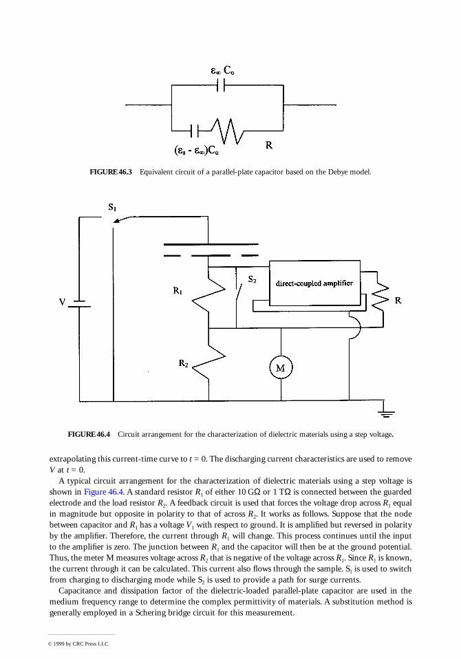
extrapolating this current-time curve to t = 0. The discharging current characteristics are used to removeV at t = 0.

A typical circuit arrangement for the characterization of dielectric materials using a step voltage isshown in Figure 46.4. A standard resistor R1 of either 10 GΩ or 1 TΩ is connected between the guardedelectrode and the load resistor R2. A feedback circuit is used that forces the voltage drop across R1 equalin magnitude but opposite in polarity to that of across R2. It works as follows. Suppose that the nodebetween capacitor and R1 has a voltage V1 with respect to ground. It is amplified but reversed in polarityby the amplifier. Therefore, the current through R1 will change. This process continues until the inputto the amplifier is zero. The junction between R1 and the capacitor will then be at the ground potential.Thus, the meter M measures voltage across R2 that is negative of the voltage across R1. Since R1 is known,the current through it can be calculated. This current also flows through the sample. S1 is used to switchfrom charging to discharging mode while S2 is used to provide a path for surge currents.

Capacitance and dissipation factor of the dielectric-loaded parallel-plate capacitor are used in themedium frequency range to determine the complex permittivity of materials. A substitution method isgenerally employed in a Schering bridge circuit for this measurement.

FIGURE 46.3 Equivalent circuit of a parallel-plate capacitor based on the Debye model.

FIGURE 46.4 Circuit arrangement for the characterization of dielectric materials using a step voltage.


In the Schering bridge shown in Figure 46.5, assume that the capacitor Cv is disconnected for the timebeing, and the capacitor Cs contains the dielectric sample. In the case of a lossy dielectric sample, it canbe modeled as an ideal capacitor Cx in series with a resistor Rx. The bridge is balanced by adjusting Cd

and Rc. An analysis of this circuit under the balanced condition produces the following relations.

(46.13)

and

(46.14)

Quality factor Q of a series RC circuit is defined as the tangent of its phase angle, while the inverse ofQ is known as the dissipation factor D. Hence,

(46.15)

For a fixed Rd, the capacitor Cd can be calibrated directly in terms of dissipation factor. Similarly, theresistor Rc can be used to determine Cx. However, an adjustable resistor limits the frequency range. Asubstitution method is preferred for precision measurement of Cx at higher frequencies. In this technique,

FIGURE 46.5 Schering bridge.

RC R

Cxd c

T

=

CC R

RxT d

c

=

QX

R C R D= = =x

x x x

1 1

ω


a calibrated precision capacitor Cv is connected in parallel with Cs as shown in Figure 46.5 and the bridgeis balanced. Assume that the settings of two capacitors at this condition are Cd1 and Cv1. The capacitorCs is then removed and the bridge is balanced again. Let the new settings of these capacitors be Cd2 andCv2, respectively. Equivalent circuit parameters of the dielectric loaded capacitor Cs are then found asfollows.

(46.16)

(46.17)

where δD = ωRd (Cd1 – Cd2)

Complex permittivity of the specimen is calculated from these data as follows:

(46.18)

and

(46.19)

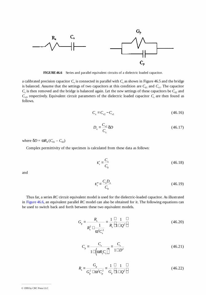
Thus far, a series RC circuit equivalent model is used for the dielectric-loaded capacitor. As illustratedin Figure 46.6, an equivalent parallel RC model can also be obtained for it. The following equations canbe used to switch back and forth between these two equivalent models.

(46.20)

(46.21)

(46.22)

FIGURE 46.6 Series and parallel equivalent circuits of a dielectric loaded capacitor.

C C Cx v2 v1= −

DC

CDx

v2

x

= δ

′ =εrx

0

C

C

′′=εrx x

0

C D

C

GR

RC

R Qp

s

s

s

s

=+

=+

2

2 2

21

1 1

1

ω

CC

R C

C

Dp

s

s s

s=+ ( )

=+1 12 2

ω

RG

G C G Qs

p

p p p

=+

=+

2 2 2 2

1 1

1ω


(46.23)

and

(46.24)

Proper shielding and grounding arrangements are needed for a reliable measurement, especially athigher frequencies. Grounding and edge capacitances of the sample holder need to be taken into accountfor improved accuracy. Further, a guard point needs to be obtained that may require balancing in somecases. An inductive-ratio-arm capacitance bridge can be another alternative to consider for such appli-cation [1].

46.2 Measurement of Complex Permittivity Using Distributed Circuits

Measurement techniques based on the lumped circuits are limited up to the lower end of the VHF band.Characterization of materials at microwave frequencies requires the distributed circuits. A number oftechniques have been developed on the basis of wave reflection and transmission characteristics inside atransmission line or in free space. Some other methods employ a resonant cavity that is loaded with thesample. Cavity parameters are measured and the material characteristics are deduced from that. A numberof these techniques, described in [3, 4], can be used for a sheet material. These techniques require cuttinga piece of sample to be placed inside a transmission line or a cavity. In case of liquid or powder samples,a so-called modified infinite sample method can be used. In this technique, a waveguide termination isfilled completely with the sample, as shown in Figure 46.7. Since a tapered termination is embedded inthe sample, the wave incident on it will be dissipated with negligible reflection and it will look like thesample is extending to infinity. The impedance at its input port will depend on the electrical propertiesof filling sample. Its VSWR S and location of first minimum d from the load plane are measured usinga slotted line. The complex permittivity of sample is then calculated as follows [5].

(46.25)

FIGURE 46.7 A waveguide termination filled with liquid or powder sample.

CG C

CC Ds

p p

p

p=+

= +( )2 2 2

2

21ω

ω

QD

C

G R C= = =1 1ω

ωp

p s s

′ =

+

−

× ( ) − −( ) ( )

+ ( )[ ]ε λ

λ

λλ

β β

βr

c

c2

2

2 4 22

2

2 22

1 1

1

S d S d

S d

sec tan

tan


and

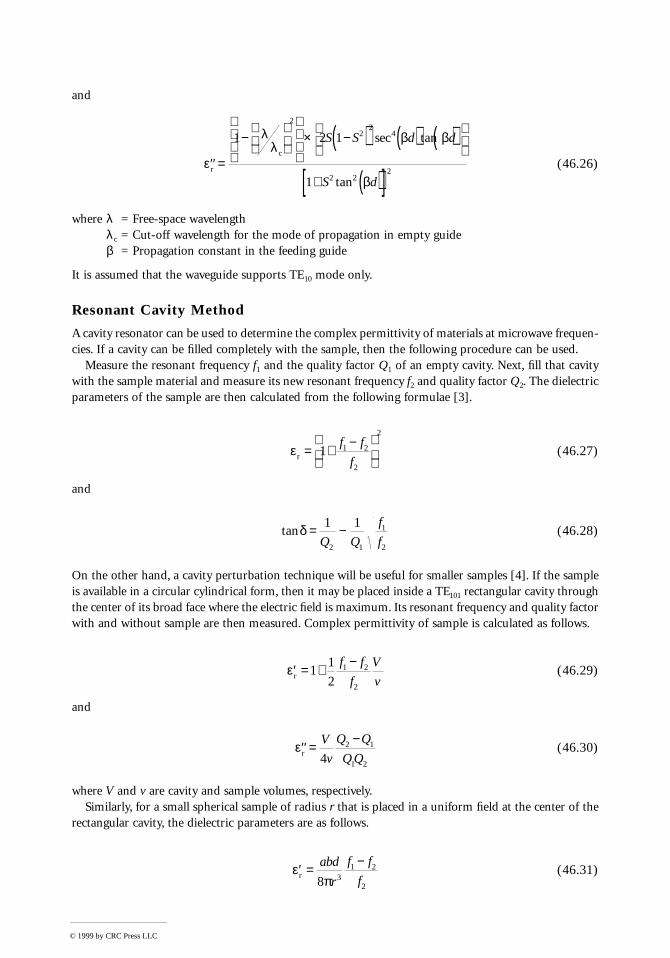
(46.26)

where λ = Free-space wavelengthλ c = Cut-off wavelength for the mode of propagation in empty guideβ = Propagation constant in the feeding guide

It is assumed that the waveguide supports TE10 mode only.

Resonant Cavity Method

A cavity resonator can be used to determine the complex permittivity of materials at microwave frequen-cies. If a cavity can be filled completely with the sample, then the following procedure can be used.

Measure the resonant frequency f1 and the quality factor Q1 of an empty cavity. Next, fill that cavitywith the sample material and measure its new resonant frequency f2 and quality factor Q2. The dielectricparameters of the sample are then calculated from the following formulae [3].

(46.27)

and

(46.28)

On the other hand, a cavity perturbation technique will be useful for smaller samples [4]. If the sampleis available in a circular cylindrical form, then it may be placed inside a TE101 rectangular cavity throughthe center of its broad face where the electric field is maximum. Its resonant frequency and quality factorwith and without sample are then measured. Complex permittivity of sample is calculated as follows.

(46.29)

and

(46.30)

where V and v are cavity and sample volumes, respectively.Similarly, for a small spherical sample of radius r that is placed in a uniform field at the center of the

rectangular cavity, the dielectric parameters are as follows.

(46.31)

′′=

−

× −( ) ( ) ( )

+ ( )[ ]ε

λλ

β β

βr

c

1 2 1

1

2

22

4

2 22

S S d d

S d

sec tan

tan

εr = + −

1 1 2

2

2

f f

f

tanδ = −1 1

2 1

1

2Q Q

f

f

′ = + −εr 11

21 2

2

f f

f

V

v

′′=−εr

V

v

Q Q

Q Q42 1

1 2

′ =π

−εr

abd

r

f f

f8 31 2

2


and

(46.32)

Where a, b, and d are the width, height, and length of the rectangular cavity, respectively. For bestaccuracy in cavity perturbation method, the shift in frequency ( f1 – f2) must be very small.

Free-Space Method for Measurement of Complex Permittivity

When a plane electromagnetic wave is incident on a dielectric interface, its reflection and transmissiondepend on the contrast in the dielectric parameters. Many researchers have used it for determining thecomplex permittivity of dielectric materials placed in free space. An automatic network analyzer andphase-corrected horn antennas can be used for such measurements [6]. The system is calibrated usingthe TRL (through, reflect, and line) technique. A time-domain gating is used to minimize the error dueto multiple reflections. The sample of thickness d is placed in front of a conducting plane and its reflectioncoefficient S11 is measured. A theoretical expression for this reflection coefficient is found as follows.

(46.33)

Where:

(46.34)

(46.35)

λ = Free-space wavelength of electromagnetic signal

Equation 46.33 is solved for εr* after substituting the measured S11. Since it represents a nonlinear

relation, an iterative numerical procedure can be used.

A Nondestructive Method for Measuring the Complex Permittivity of Materials

Most of the techniques described thus far require cutting and placing a part of sample in the test fixture.Sometimes, it may not be permissible to do so. Further, the dielectric parameters can change in that process.It is especially important in the case of a biological specimen to perform in vivo measurements. In one suchtechnique, an open-ended coaxial line is placed in close contact with the sample and its input reflectioncoefficient is measured using an automatic network analyzer [7, 8]. As recommended by the manufacturers,the network analyzer is calibrated initially using an open-circuit, a short-circuit, and a matched load. Thereference plane is then moved to the measuring end of the coaxial line using a short-circuit.

Assume that a and b are inner and outer radii of the coaxial line, respectively. ω is the angular frequency;

µ0 and ε0 are the permeability and permittivity of the free space, respectively, k = ω is the

wavenumber in material medium. Admittance of the coaxial aperture in contact with material medium

is as follows.

′′=π

−

εr

abd

r

Q Q

Q Q16 32 1

1 2

SjZ d

jZ d11

1

1=

( ) −

( ) +d d

d d

tan

tan

β

β

Zd

r

=∗

1

ε

βλ

εd r= π ∗2

µ ∗

0 0 rε ε


(46.36)

where Eρ(ρ′,0) is radial electric field intensity over the aperture. It is evaluated from the following integralequation.

(46.37)

Where:

(46.38)

(46.39)

(46.40)

(46.41)

(46.42)

The eigenvalues γn are solutions to the following characteristic equation:

(46.43)

Jn and Yn are Bessel functions of the first and second kind of order n, respectively. εl is the dielectricconstant of the insulator and kl is wavenumber inside the coaxial line.

Equation 46.37 is solved numerically using the method of moments. A numerical root-finding proce-dure, such as the Muller’s method, is used to solve Equation 46.36 for the complex wavenumber k.Complex permittivity, in turn, is determined from the following relation.

(46.44)

Y

E d b a

a

bL

0

0 l

=

′( ) ′

− π

µ ( )

∫

2

0

2

ρ ρ ρ ε ε, ln

10 0

0π

+ ′( ) ′( ) ′ ′ =π

′( ) ′ ′ ′( ) −( )′∫ ∫ ∫

∗ π

ρωε ε ρ ρ ρ ρ ρ ωε ε ρ ρ ρ φ φρ ρj E K d

jE d

jkr

rd

a

b

a

b

l o cr 0, , , cos

exp

r = + ′ − ′ ′( )ρ ρ ρρ φ2 2 2 cos

K jA

n

c

n n

n n

ρ ρφ ρ φ ρ

β, ′( ) =

( ) ′( )=

∞

∑ 2

0

φ γ γ ρ γ γ ρn 0 n n 0 n n= ( ) ( ) − ( ) ( )Y a J J a Y1 1

βγ

γ

γγn

l n

n l

l n

l n

=−

− −

><

k

j k

k

k

2 2

2 2

AJ a

J bn A

b

an

n2

02

n

02

n

02

2

221 0=

π( )( ) −

> =

γ

γ

γ ; ln

J b Y a J a Y b0 n 0 n 0 n 0 nγ γ γ γ( ) ( ) = ( ) ( )

εω εr

0 0

∗ =µk2

2


Defining Terms

Electric dipole: A pair of equal and opposite electric charges separated by a small distance.Isotropic material: A material in which the electrical polarization has the same direction as the applied

electric field.Electric polarization density: The average electric dipole moment per unit volume.Electric susceptibility: A dimensionless parameter that relates the polarization density in a material

with electric field intensity.Electric flux density: A fundamental electric field quantity that is related to volume density of free

charges. It is also known as the electric displacement.Time domain field: A field expressed as a function of time. It is a real function that is dependent on

time and space coordinates.Frequency domain field: A phasor quantity (a complex function in general) that depends on space

coordinates. The time dependency is assumed to be sinusoidal.Displacement current density: It represents the time rate of change of electric flux density.Conduction current density: Current per unit area caused by conduction of charge carriers.Dielectric constant: A dimensionless constant that represents the permittivity of a material relative to

the permittivity of free space.Loss tangent: A ratio of the imaginary part to the real part of the complex permittivity of a material.Relaxation time: It represents the time taken by a charge placed inside a material volume to decay to

about 37% of its initial value.Quality factor: A dimensionless quantity that represents the time average energy stored in an electrical

circuit relative to energy dissipated in one period.Dissipation factor: It is the inverse of the quality factor.Voltage standing wave ratio (VSWR): Defined as a ratio of maximum voltage to the minimum voltage

on a transmission line.Reflection coefficient: Defined as a ratio of reflected phasor voltage to that of incident phasor voltage

at a point in the circuit.

References

1. A. R. Von Hippel, Dielectric Materials and Applications, Cambridge, MA: MIT Press, 1961.2. N. E. Hill, W. E. Vaughan, A. H. Price, and M. Davies, Dielectric Properties and Molecular Behaviour,

London: Van Nostrand Reinhold, 1969.3. M. Sucher and J. Fox (eds.), Handbook of Microwave Measurements, Vol. II, Brooklyn, NY: Poly-

technic Press, 1963.4. R. Chatterjee, Advanced Microwave Engineering, Chichester, U.K.: Ellis Horwood Limited, 1988.5. D. K. Misra, Permittivity measurement of modified infinite samples by a directional coupler and

a sliding load, IEEE Trans. Microwave Theory Technol., 29, 65-67, 1981.6. D. K. Ghodgaonkar, V. V. Varadan, and V. K. Varadan, A free-space method for measurement of

dielectric constants and loss tangents at microwave frequencies, IEEE Trans. Instrum. Meas., 38,789-793, 1989.

7. A. P. Gregory, R. N. Clarke, T. E. Hodgetts, and G. T. Symm, RF and microwave dielectric mea-surements upon layered materials using a reflectometric coaxial sensor, NPL Rep., DES 125, UK,March 1993.

8. D. Misra, On the measurement of the complex permittivity of materials by an open-ended coaxialprobe, IEEE Microwave Guided Wave Lett., 5, 161-163, 1995.


permittivity

Documents