phase multipath estimation for global positioning system (gps
TRANSCRIPT
Phase Multipath Estimation for Global Positioning System (GPS)
Using Signal-to-Noise-Ratio (SNR) Data
byFrancesca Scir6 Scappuzzo
B.S. and M.Eng., Summa Cum Laude , Electrical EngineeringUniversity of Catania, 1989
Submitted to the Department ofEarth, Atmospheric, and Planetary Sciences
in Partial Fulfillment of the Requirements for the Degree of
Master of Science in Earth and Planetary Sciences
at theMASSACHUSETTS INSTITUTE OF TECHNOLOGY
May 1997
@ 1997 Massachusetts Institute of TechnologyAll rights reserved.
Signature of AuthorDepartment of Earth, Atmospher(icand Planetary Sciences
May, 1997
Certified byThomas A. Herring
Associate Professor of GeophysicsThesis Supervisor
Accepted by
ARCHIVES Thomas H. JordanDepartment Head
, -tj , 8 '.-,.7AV(-


This thesis is dedicated to
Prof. Sebastiano BarbarinoAssociate Professor of Electromagnetics
University of Catania, Italy
... perche' il Suo amore per lo studio e per la scienza,la Sua encomiabile dedizione all'insegnamento e
la Sua grande umanita'
siano da esempio ai Suoi studenti e colleghi
ed ispirino le generazioni a venire ...

Phase Multipath Estimation for Global Positioning System
(GPS) Using Signal-to-Noise-Ratio (SNR) Data
byFrancesca Scire Scappuzzo
Submitted to the Department of Earth, Atmospheric, and Planetary Sciences
in Partial Fulfillment of the Requirements for the Degree of
Master of Science in Earth and Planetary Sciences
Abstract
A method for the estimation of GPS multipath phase error is proposed. Becausethe Signal-to-Noise-Ratio (SNR) of the GPS measurements is strictly related to themultipath phase error, the algorithm implemented manipulates the SNR of thereceived GPS signal itself to perform the estimation. No additional informationabout the geometry of the surroundings of the receiving station or the weatherconditions at the time of acquisition are needed. The scattering phenomenon isgenerally due to the composition of several single multipath contributions, each onecharacterized by a specific frequency. The algorithm takes advantage of thisproperty to decompose the variations of the SNR into individual components in aniterative procedure. The contributions due to each frequency are then superimposedto obtain the total multipath phase error.
The algorithm was applied to several data sets affected by strong multipath to testthe performance of the method. Spectral and statistical analyses were performed tocompare the observed phase residual obtained from the GPS measurements and theestimated multipath phase error retrieved by the algorithm.
In most of the cases analyzed, a broad-band coherence function between theobserved phase error and the estimated multipath phase error was found in presenceof strong multipath. This suggests that the effects of multiple reflectors are correctlyretrieved by the proposed algorithm.

The set of data which show the highest coherence have multipath frequenciesbetween 0.001 and 0.01 Hz. Therefore, the estimation algorithm presents goodperformances when the reflectors are located at a distance between 5.50 m and 55.0m from the receiving antenna, for an elevation angle of about 10' and a rate of changeof the elevation angle of 0.1 mrad/sec. The high coherence is confirmed by thestatistical analysis, which shows a significant decrease of the RMS of the phaseresidual after the multipath correction.
At lower frequencies it was found that the performance of the algorithm dependson the receiver type, the antenna gain and the weather conditions.
Thesis supervisor: Thomas A. HerringTitle: Associate Professor of Geophysics

Contents
Introduction 9i.1 Objectives ..................................................
1.2 Outline ..................................................... II
2 Multipath Modeling in phasor space. Relationship between
Multipath Phase Error and SNR 132.1 Introduction ................................................. 13
2.2 Multipath representation ...................................... 52.2.1 Multipath Modeling in the Phasor Space .................. . 52.2.2 Relationship between the signal strength and the multipath
phase error ........................................... 18
2.2.3 The SNR and the measured signal strength, Ac ........... 212.2.4 Multipath frequency ................................... 222.2.5 Influence of the Reflection coefficient on the multipath
phase error ........................................... 24
2.2.6 Antenna Gain contribution to the Signal strength ........... 312.3 GPS receivers in presence of multipath ......................... 35
2.3.1 GPS receivers ......................................... 352.3.2 The DLL and PLL in the presence of multipath ............ 362.3.3 L2 signal processing in the presence of AS (Anti-spoofing) .... 37
3 Description of the algorithm for the Multipath Phase Error
Estimation from the SNR data 39
3.1 Introduction ................................................ 39
3.2 Errors in the GPS Phase Measurements ....................... 40
3.3 Multipath Phase Error Estimation Algorithm ..................... 42
3.3.I Antenna Gain removal .................................. 42
3.3.2 Data Segment Selection ................................. 46
3.3.3 Spectral Decomposition of the SNR ...................... 46

4 Statistical and Spectral Analysis of estimated and observedGPS phase errors
4.1 Introduction ................................................
4.2 Data Preprocessing .. .....................................
4.3 Spectral Analysis ........................................
4.3.1 Multipath Frequency ...............................
4.3.2 Power Spectral Density .............................
4-3.3 Auto Correlation and Cross Correlation ...................
4.3.4 Auto and Cross Spectral Density Function .................
5.3.5 Coherence Function ..................................4-4 Statistical Analysis of GPS Phase Residual ......................
Applying the method ofmultipath estimation to GPS data
5.1 Introduction ..........................................
5.2 Description of the GPS stations and the data sets analyzed .........
5.2.1 The Tien-Shan data ....................................5.2.2 The LIGO data .. ....................................5.2.3 The IAP data ........................................
5.3 Multipath Estimation and Results of Spectral Analysis ............
5.3.1 KKAU and MANA ..................................5.3.2 Station 0036 and 0028 (TRIMBLE 4oooSSE) ..............
5.3.3 COSE and GS29 ....................................
5.4 Multipath Estimation and Results of Statistical Analysis ............
6 Conclusions
53.53-54.55.55.55
.56
.58
.59
.60
.63
.64.64
.65
.65
.67
.67
.71
.74
.77
79
REFERENCES .................................................... 83
APPENDICES .................................................... 90
A. Plots of spectral analysis
B. Tables of statistical analysis
C. Matlab Algorithms

Chapter 1
Introduction
Over the last decade the Global Positioning System (GPS) has become a very
useful tool for several scientific and civilian applications, playing a leading role in
geodynamic studies, from a local to a global scale. High accuracy GPS is being
extensively used in large scale dynamics of the Earth, such as plate tectonics, Earth's
rotation studies, sea-level change, post-glacial rebound, tidal effect and sea-surface
topography.The extensive utilization of GPS in geosciences is mainly due to the recent
significant improvements of the techniques involved in high-accuracy GPS
positioning. The relatively low costs of post processing software and new GPS
receivers and their availability and portability during field work, make the GPS a very
convenient and useful instrument. The international collaboration in the GPS
scientific community is also sensibly contributing to such a wide diffusion of the
system.
However, even though research and technology on high accuracy GPS positioning
have rapidly developed, there is still a broad range of critical issues that scientists and
engineers need to exploit. Most of the new questions arise from the fact that the
fields of application and the accuracy required today for positioning instruments,

have greatly overcome the purposes for which GPS was originally designed,
producing a series of new challenging riddles.
One of the main problems to be faced when performing high-precision GPS
measurements is the error in positioning due to the occurrence of multipath. This
phenomenon is caused by the interference of multiple reflections with the direct
EM signal transmitted by the satellite, and represents a considerable source of error
in the GPS carrier phase observations (fig. 1.1).
The level and characteristics of the noise deriving from multipath depends upon
the geometry of the surrounding of the receiving antenna (presence of buildings,
trees, towers, and the mount itself), the reflectivity of nearby reflectors, the elevation
angle of the satellite at the time of acquisition, and other parameters which might
sensibly change with weather conditions and time.
GPS satellite
rface
GPS receiver
Fig. 1.1: GPS multipath phenomenon
Due to the variability of the parameters involved, it is very difficult or evenimpossible to predict multipath with sufficient accuracy using a deterministicapproach such as electromagnetic modeling or analog techniques.
1.1 Objectives
The objective of the study presented in this thesis is to estimate the multipathphase error from the SNR (Signal-to-Noise-Ratio) data, without using any a prioriinformation about the location of the receiving station, the weather conditions andthe geometry of the surroundings. This method manipulates the SNR of the
received signal, which in GPS data processing is usually only used as an indicator ofthe data reliability and is not used for the positioning itself.
In order to test the performance of the estimation algorithm for different sites and
different GPS receiver types (Ashtech Z-12, Trimble SSE and SSI, and Turbo-Rogue SNR8000), the method was applied to a large number of data sets, chosen forthe strong multipath in the phase error measurements.
1.2 Outline
In chapter 2 a mathematical representation of the multipath phenomenon is
derived. The dependency of the multipath phase error on the SNR, the antenna
gain, the multipath frequency and the reflection coefficient of the reflecting surface
is discussed.
After a brief introduction on the basic operation of GPS receivers, chapter 3
focuses on how a GPS signal corrupted by multipath is processed by differentreceivers.
The algorithm for the estimation of the multipath phase error from the SNR data
is described and discussed in chapter 4.

In order to test how well the estimated multipath phase error matches the phase
error observed in the GPS measurements, statistical and spectral analyses were
performed. The theory of these analyses is presented in chapter 5.
The estimation algorithm was applied to several data sets affected by significant
multipath effects. Its performance was studied comparing the results obtained in
the different cases. The results of this analysis are discussed in chapter 6 and the
conclusions are drawn in chapter 7.
The plots relevant to the estimation and spectral analysis of the 42 data sets
studied are collected in appendix A. In appendix B, the tables containing the
results of the statistical analysis are shown. The matlab programs implemented for
the analysis can be found in appendix C.

Chapter 2
Multipath Modeling in phasor space.
Relationship between Multipath
Phase Error and SNR
2.1 Introduction
The correction of GPS multipath phase errors is one method of improving theaccuracy of GPS measurements. In literature several approaches for GPS multipathcorrection can be found. Hajj (1990) developed an algorithm to produce maps of the
multipath for a given environment around the receiving antenna. Unfortunately,multipath errors are very sensitive to parameters such as the geometry or the
reflection coefficient of nearby reflectors which strongly depend on the particular
weather condition and season. This limits the efficiency of this method in
predicting the multipath effects with time.

An easy solution to the multipath problem consists in selecting a proper site, far
from possible reflectors. However in many applications it is not possible to choose
the site for the GPS positioning. Other ways to minimize multipath consist in the
design of antennas which reduce back-plane gain. Receivers manufacturers are
trying to correct multipath using particular selections of the cross-correlation
function. A branch of research on GPS multipath, is now oriented toward the
analysis of the data itself for the error estimation in post-processing mode
(Georgeadu and Kleusberg, 1988). One new promising method is to compute the
multipath error by using the SNR, as in Axelrad et al., (1994).
The circumstances in which the measurements are acquired are usually recorded
on the log sheets of the GPS measurements, which report the geometry of the site,the weather conditions during the data acquisition, etc. But to gather the correct
information about the GPS receiver surroundings and relevant measurements can be
extremely difficult and inefficient. The possibility to correct for multipath
contribution to the phase error without a priori information is particularly important
for applications that require networks of GPS stations distributed over large areas on
the globe, such as geosciences.
The multipath phase error estimation algorithm proposed in this thesis makes use
of the SNR of the data itself, without the need for additional information about the
geometry and conditions of the surrounding of the receiving antenna. The methodfor the estimation of 50, is based on the spectral analysis of the SNR information
provided by the GPS receiver. We assume that the multipath effects are due to
multiple reflectors, which will each have a particular frequency. Through spectral
decomposition of the SNR we can isolate the contributions of each reflector.
Inverting for the phase error of all the single contributions and superimposing the
results together, we obtain the total multipath correction (total multipath phase error).
This chapter is devoted to the definition of the theoretical model of the multipath
phenomenon used in the multipath phase error estimation algorithm. The importantrelationship between the multipath phase error to be estimated , 80, and the SNR
data, used as input of the estimation algorithm, is discussed in section 2.2.2. The
dependency of the signal strength (A) and the multipath phase error (&0) on the
phase of the multipath signal, on the multipath frequency and on the reflection

coefficient of the reflecting surface is derived in sections 2.2.4 and 2.2.5. The
influence of the antenna gain on the signal strength is shown in sections 2.2.6.
2.2 Multipath representation
2.2.1 Multipath Modeling in the Phasor Space
In this section the mathematical model of the multipath phase error used for the
estimation algorithm is derived.The multipath phase error, 80D, is defined as the angle between the direct signal,
Sd(t), and the total received signal, Sc(t), which is the composition of the direct signal
and the multipath signal, Sm(t). The signals can be written as:
i(Co't + Od)Sd (t)= Ad (t).e [2.1]
Sm (t) = Am (t).e 't [2.2]
i t't+mi
= A ei( t' t + d ) (t . [2.3]Sc (t) = Ac (t) -ei( O = Ad (t) + mi [2.3
where:Ad = Amplitude of the direct signal
Ami = Amplitude of the i-th multipath contribution
kA= Amplitude of the total measured signal
Od = Phase of the direct GPS signal.4mi= Phase of the multipath signal due to the i-th reflector.

OC = Phase of the total measured GPS signal.o = 2 7 f and f is the carrier frequency (LI or Lz)
In figure 2.1 the total signal measured by the receiver, the direct signal and the
signal due to the composition of several multipath reflections are shown in the
phasor space.
Figure 2.1: Phasor diagram of the GPS signal. 80 is the multipath phase error
in presence of a single reflector. It depends on the amplitude
(Am=Rf Ad) and phase (Om=Od+fmt) of the multipath phasor.
In the phasor space the signals of fig. 2.1 can be written as:
A = Adl ei d
AmmAm = Ami. ie
i-A = AcI e e
Om, = Od + Pi = d + (fm, t)
[2.4]
[2.5]
[2.6]
im

where:i = Phase of the i-th multipath signal with respect to the direct GPS
signal
fni = Multipath frequency relevant to the i-th contribution, such that
Pi =fmi t +0oi
0oi = Phase of the i-th multipath signal with respect to the direct GPS
signal at the initial time t=0.80- Total multipath Phase Error
Rfi= Reflection coefficient for the i-th reflector. IAmil = Rf IAdl.
The composite signal is given by:
c = d +Ami = Ad .ed + + R Ade( d + i) [2.7]
The multipath phase error depends on the amplitude of the multipath signal
and its phase. Because 3 changes with time as a function of the multipath frequency
fm, the multipath phasor spins around the tip of the direct signal, producing positive
and negative values of the phase error 80.
If we rotate the diagram of figure 2.1 as in figure 2.2, so that 4d -0 and Ad is along
the Real axis, the total strength of the received signal and the phase error can be
written as:
lAc = Ad (1 + Rfifi cosi) 2 +(.Ri, sini )2 [2.8]V+ýi [28
[2.9],,
tcp =

Im(Ac
Figure 2.2: Phasor diagram 2.1 for Od =0 and Ad real.
2.2.2 Relationship between the signal strength and the
multipath phase error.
The amplitude of the composite signal Ac is related to the total phase error, 80through the angle P3, phase of the multipath vector Am with respect the direct signalAd (fig. 2.1, formulas [2.8] and [2.9]).
To describe the phenomenon, we consider the simple case of a single reflector(i=1). (The same theory is applicable to multiple reflections, considering thesuperposition of the multipath contribution).
Re

Because the multipath signal rotates around the tip of the direct signal , withfrequency fim, the amplitude of Ac oscillates between a maximum value Ad +Am and a
minimum value, Ad -Am. The change in amplitude of Ac due to the rotation of Am
can be easily deduced from 2.3. Ac is plotted as function of time for different values
of 1. Every time A, presents a maximum ( for 3=0' ) or a minimum ( for 1=180" ), themultipath phase error is zero. The maximum phase error occurs for P=90" and
1=270'. (see fig. 2.1 and formula [2.9] ).In table 2.1 the values of A, and 6Q as functions of P are summarized . It is
important to notice that Ac can assume the same amplitude for different values of 1(for example for P=90" and 1=270'). This produces an uncertainty in thedetermination of the sign of 86, which represent a very critical problem in the
multipath phase error estimation algorithm.
Ac =SNR
t
=0° 13=900 1-1800
Figure 2.3: Variation of Ac with the time, as function of the angle 3.

/= Phase error
A =A +Ac d
(Max SNR)
0 = f t = 900 =* Phase error
SNR
+ = tan - 1 [m (Max 8I)
A = A 2 + A 2c d m
= f.t = 180 0 = Phase error
Ac = Ad - A mc d m (Min SNR)
/ = fQt = 2700 = Phase error
SNR
- 31 = -tan - 1 (Min &0)AA
A = Ad 2 +A 2c d m
Table 2.1 : Signal strength, Ac and multipath phase error, 80, as functions of 3.In section 2.2.3 it is shown that Ac and the Signal-to Noise-Ratio (SNR)
actually represent the same quantity in the GPS receiver processing.The relationship between the SNR and 80, is crucial for the phase
error estimation algorithm presented in chapter 4.
SNR
50 = 0
SNR
,= fl t = 00 30 = 00
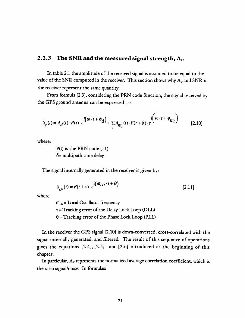
2.2.3 The SNR and the measured signal strength, Ac
In table 2.1 the amplitude of the received signal is assumed to be equal to thevalue of the SNR computed in the receiver. This section shows why Ac and SNR in
the receiver represent the same quantity.
From formula [2.3], considering the PRN code function, the signal received bythe GPS ground antenna can be expressed as:
-4("t+ d) i(j -t+ mi)Sc (t) = ad(t) -P(t) ei + .Ami (t) -P(t + 8) e [2.10]
where:
P(t) is the PRN code (±1)8- multipath time delay
The signal internally generated in the receiver is given by:
S (t) = P(t + ). -e( t + ) [2.11]
where:
oo = Local Oscillator frequency
, = Tracking error of the Delay Lock Loop (DLL)
0 = Tracking error of the Phase Lock Loop (PLL)
In the receiver the GPS signal [2.10] is down-converted, cross-correlated with the
signal internally generated, and filtered. The result of this sequence of operations
gives the equations [2.4], [2.5] , and [2.6] introduced at the beginning of this
chapter.
In particular, A, represents the normalized average correlation coefficient, which is
the ratio signal/noise. In formulas:
= normalized corr. coeff. = SNR
where:SNR = Signal Strength [2.13]
Noise
However, the precise normalization used in the receiver is not always the same, butdepends on the particular manufacturer. We can assume that the values of thecorrelation coefficient are normalized by the expected correlation coefficient when
only noise is present.It follows that the SNR is equivalent to the signal strength of the total composite
signal, Ac. Therefore, all the properties we found for Ac are valid also for the SNR.In table 2.1 the values of the SNR and 601 as function of P were summarized.
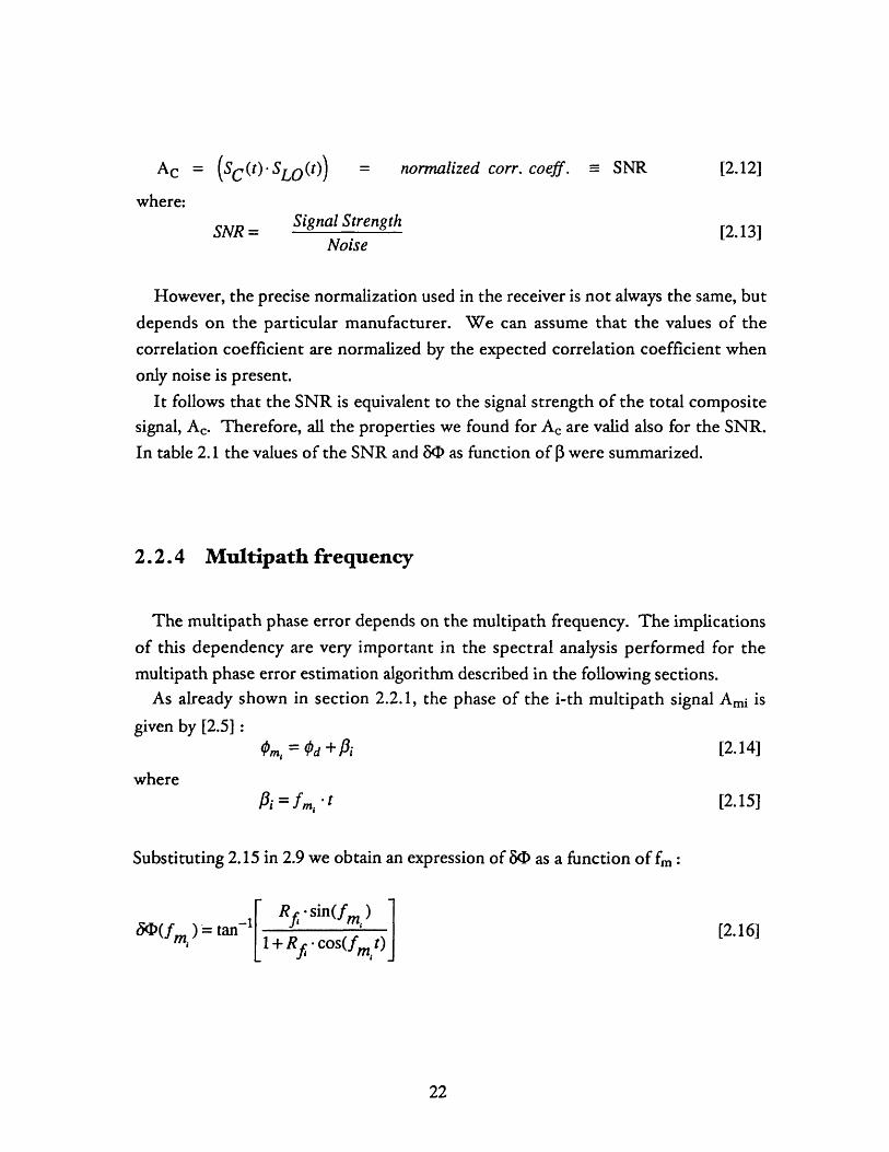
2.2.4 Multipath frequency
The multipath phase error depends on the multipath frequency. The implicationsof this dependency are very important in the spectral analysis performed for themultipath phase error estimation algorithm described in the following sections.
As already shown in section 2.2.1, the phase of the i-th multipath signal Ami is
given by [2.5] :Om, = d +f [2.14]
wherefi = i, " t [2.15]
Substituting 2.15 in 2.9 we obtain an expression of 8(1 as a function of fm:
(f )= tan-1 +Rfco t) [2.16]m+R -cos(fmt)
AC = SC (t) -SLO (t)) [2.12]

The frequency of the i-th multipath error depends on the carrier frequency, the
distance of the i-th reflector and the receiving antenna, the rapidity of the change in
elevation angle of the satellite and the elevation angle.
For an horizontal reflector at distance hi below the antenna, the multipath
frequency is (Leich, 1995):
i, = -. sin y- [2.17]
where:
h = Distance between the antenna phase center and the reflector
S= Wavelength
Nr = Zenith angle = (90' - Elevation angle)
One of the consequences of equations [2.16] and [2.17] is that 80 varies with time
due to changes of the elevation angle, as the satellites rises or sets.
Moreover, the multipath phase error, 80, presents a particular frequency
component fmi for each reflector located at a certain height below hi from the
receiving antennas. From [2.8] and [2.9] we can deduce that Ac (=SNR) and 8o
present the same spectral content, being both functions of 13=fmt.
Therefore, the multipath phase error 50i due to a particular reflector can be
identified by the spectral analysis of the total signal strength Ac (SNR).
The method for the estimation of the total composite 8I, is based on the spectral
analysis of the SNR information provided by the GPS receiver. We assume that the
multipath effects are due to multiple reflectors, which will each have their own
frequency. Through spectral decomposition of the SNR we can isolate the
contributions of each reflector. Inverting for the phase error of all the single
contribution and adding them together, we obtain the total multipath correction, as it
will be shown in more detail in chapter 4.

2.2.5 Influence of the Reflection coefficient on the multipath
phase error
The multipath phase error 80i is a function of the Reflection Coefficient Rf, as
shown in formula [2.9]. The reflection coefficient depends on the electromagneticcharacteristics of the reflecting surface, such as permittivity (e), permeability (g), and
conductivity (d). It depends also on the frequency of the electromagnetic signal and
the elevation angle of the satellite 0.In this section we derive the expression of the reflection coefficient Rf for one
single reflector as a function of E, gt, and a, and discuss how these electromagnetic
properties of the reflector influence the multipath phase error.The geometry of our problem is shown in figure 2.4, where Einc is the incident
electromagnetic wave transmitted by the GPS satellite, Et is the EM wave refracted
into the material and Er is the EM wave reflected by the surface.
Ci.
z
Figure 2.4: Electromagnetic plane waves propagating in medium 1 (air) and
medium 2 (reflector).
I A--J:. & A--J: . -
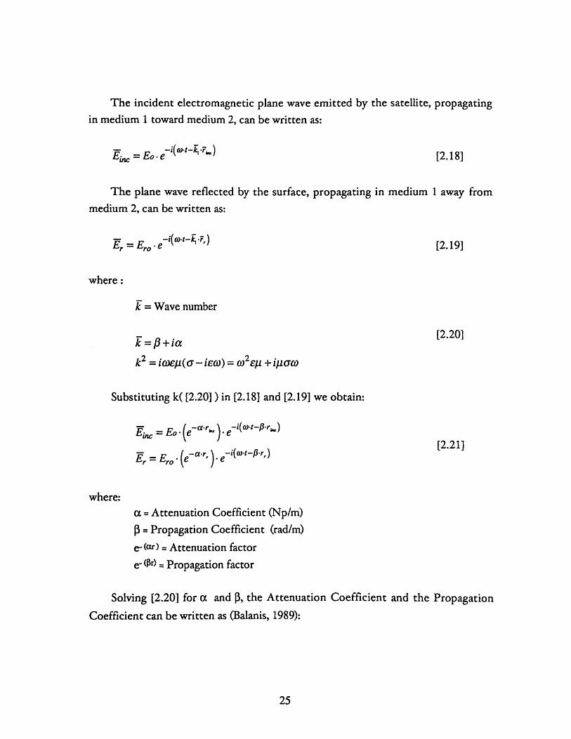
The incident electromagnetic plane wave emitted by the satellite, propagatingin medium 1 toward medium 2, can be written as:
E = Eo e- i(t- •.r ) [2.18]
The plane wave reflected by the surface, propagating in medium 1 away frommedium 2, can be written as:
Er = Ero .e- i(• - v) [2.19]
where :
k = Wave number
F= /3+ia [2.20]
k2 = ie(-ieW) = o 2E + iaUT
Substituting k( [2.20]) in [2.18] and [2.19] we obtain:
Ei, = Eo -(e-a-r, ). e-i('r, [2.21,)
Er = Ero (e-a.r, ). e-i(Otpr,)
where:a = Attenuation Coefficient (Np/m)
p = Propagation Coefficient (rad/m)
e-(ar) = Attenuation factor
e- (r) = Propagation factor
Solving [2.20] for a and 0, the Attenuation Coefficient and the Propagation
Coefficient can be written as (Balanis, 1989):

S= o 1+ 22 1 [2.22]2 E2)2
0_ a2 + [2.23]
The term e - (ar) represents the attenuation of the electromagnetic wave in the
material, and the exponential e -j(r) represents the propagation term. Note that for
air (medium 1 where the GPS signal propagates), a 1= 0, and therefore e -(ar) s 1.
The electric fields of the incident and reflected wave can be decomposed in a
component perpendicular to the plane of incidence (horizontal polarization) and a
component parallel to the plane of incidence (vertical polarization). In formulas:
Horizontal Polarization:
-h [Eh e-i',(xsinO,+zcosO,)[2.24]
Eh h E -i,(xsin,-zcos)[2.2
Vertical Polarization:
-. = [E . e-iPj(xsin°j+zCs cos] O- ,sin 0) 2.25
Er = [E',0 e-iP,(xsin,-zcos,)] (ycos Or + isin Or)
where:
0i = Incidence angle
Or = Reflection angle
The Fresnel Reflection Coefficient for the horizontal (perpendicular)
polarization is given by:

Erh =2 COS Oi - 071 COS 8 t
EihN, 772 COS Oi 771 COS Ot
cos 8- 1172
cos ei + .1072
[2.26]
The Fresnel Reflection Coefficient for the vertical (parallel) polarization is given
by:
S= Er -171 cOS 8i + 72 COS OtEi 71 cos Oi + 772 COS Ot
-cos Oi + _2171
cos 90 + 02
where:
Ot = Refraction angle
= Intrinsic impedance of the medium.
The angles of Incidence, Reflection and Refraction, of fig. 2.4 are related by
the Snell's laws:
O0 = Oik1 sin Oi = k2 sin 8,
Snell's law of reflection
Snell's law of refraction
[2.28][2.29]
The Intrinsic Impedance of a medium is given by:
for dielectric materials
{ iouM for conductive materials0'+i oe
[2.30]
In our case, the medium 1, where the incident and reflected signal propagate, isair. For air the intrinsic impedance can be considered as the one for dielectricmaterials.
[2.27]
EH1=-=H

Depending on the electromagnetic characteristics of the reflector, we can
distinguish 3 cases, which represent 3 different categories of materials.
Case I: Good Dielectrics
If the reflector (medium 2) is a good dielectric at the frequency of the GPS
signals (Microwaves) we obtain:
'222 2 << 1E2 02
=71 = •1 -72 2
and Rf =f
-cos ei - cIL cos o~n_ •E2 E
C2 1
-I COS 0 + 12COS +62 re,2
Scos o,
Case II: Quasi-conductors
If he reflector is a quasi-conductor at the frequency of the GPS signals,it follows that:
and Rf = <
iW o s2 C/ t cos7" + i0E2 OS
iRh 2 2 osO
Scos Oi + cos 82 2___ /1
-cos O + i92 cos ORV= a 2 + i(82
cosBi + i cos O,Ei "2 + i082
2
E2 2 1
,22(02
-1i =
772a 2 + itoE2
cos i +R
Inh =
In this case the reflector is not a good dielectric, nor a good conductor, havinginter medium characteristics. The reflection coefficients (horizontal and vertical)can be determined using the general formulas [2.26] and [2.27] , respectively.
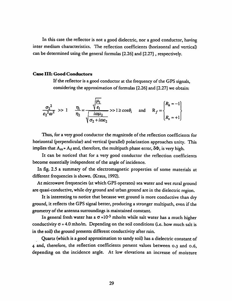
Case III: Good Conductors
If the reflector is a good conductor at the frequency of the GPS signals,considering the approximation of formulas [2.26] and [2.27] we obtain:
>> 1 2 >16220)2 72
rRh -1>> 1 cos9. and Rf =
R, +1
Thus, for a very good conductor the magnitude of the reflection coefficients forhorizontal (perpendicular) and vertical (paralleD polarization approaches unity. Thisimplies that Am Ad and, therefore, the multipath phase error, 80, is very high.
It can be noticed that for a very good conductor the reflection coefficientsbecome essentially independent of the angle of incidence.
In fig. 2.5 a summary of the electromagnetic properties of some materials atdifferent frequencies is shown. (Kraus, 1992).
At microwave frequencies (at which GPS operates) sea water and wet rural groundare quasi-conductive, while dry ground and urban ground are in the dielectric region.
It is interesting to notice that because wet ground is more conductive than dryground, it reflects the GPS signal better, producing a stronger multipath, even if thegeometry of the antenna surroundings is maintained constant.
In general fresh water has a o =10-3 mho/m while salt water has a much higherconductivity a = 4.0 mho/m. Depending on the soil conditions (i.e. how much salt isin the soil the ground presents different conductivity after rain.
Quartz (which is a good approximation to sandy soil) has a dielectric constant of
4 and, therefore, the reflection coefficients persent values between 0.3 and 0.6,depending on the incidence angle. At low elevations an increase of moisture

content might increase the reflection coefficient of 60%, so that the reflectioncoefficient is almost unity. (R 1).
This example suggests that the weather conditions might influence theperformance of GPS measurements, because of the different multipath environmentthey can produce.
M = 6
5
4
3
2
1
0
-1
-2
-3
-4
-5
.V = 1 2 3 4 5 6 7 8 9 10 11 12 13 14 15 16 17Frequency = 10v Hz
Fig. 2.5 Ratio ao/w as a function of frequency for some common media.
At Microwave frequencies the most of the media shown are in thequasi-conductive region (urban ground, rural ground, sea water), with theexception of copper, which, being a metal, is a very good conductor evenat higher frequencies, up to the Visible spectra. (Kraus, 1992)
-4
-5

2.2.6 Antenna Gain contribution to the Signal strength
In formula [2.8], Ac is described as a function of Ad ,Rf and P. We already
discussed its dependency on Rf and P. To complete this theoretical analysis of 80
and Ac we need to study how the amplitude of the direct signal, Ad is influenced by
Ac. The direct signal sent by the transmitting antenna, Ad, is a function of the GPS
satellite antenna pattern, as will be discussed in section [2.2.6.1]. The total signal
measured by the receiver, Ac, depends on the receiving antenna pattern (section
[2.2.6.2] ).
22.6.1 GPS Transmitting antenna gain and its influence on Ad
The purpose of a GPS transmitting antenna is to illuminate the Earth surface in
the field of view of the satellite with a uniform strength.
The GPS transmitting antennas present patterns properly shaped to
compensate for the path loss occurring at low elevation angles. The path loss of the
signal is a function of the distance between the antenna phase center and the point
on the surface of the Earth where the GPS receiver is located. The path loss is
minimum when the satellite is at 90 ° elevation angle (at zenith) and is maximum
when the satellite is at 0" elevation angle (at the horizon). A comparison between the
pattern of an ideal antenna pattern and a typical GPS antenna is shown in fig. 2.6.
The edge of the Earth in view subtends an angle of approximately 27.74 * from
the GPS satellite altitude. The satellite antenna pattern extends behind the edge of
the Earth, as shown in fig. 2.7. The transmission power from the satellite is not
uniform with the angle of bore-sight of the satellite. The beam transmits more
power toward the Earth's limbs, so that low elevation angle measurements on the
ground will see more power.
The direct signal Ad is a function of the signal strength transmitted by the
satellite, Atrans , and also of the transmitting antenna pattern Gt(O,0), where 0 and 0
are elevation angle and azimuth of the satellite, respectively:
Ad = Ad(8,0) = Atrans Gt(0, ) [2.31]

-2.1 dB
DEAL ANTENNAPATTERN
Figure 2.6: Comparison between the antenna patterns of an ideal GPStransmitting antenna and a typical one (Parkinson, 1996).
f a 1227 MHz: a = 45", 225*L2 FREQUENCY
72 36 0 36 72f = 1575 MHz: w = 450, 2250
L1 FREQUENCY
Figure 2.7: Antenna patterns of a GPS transmitting antenna at LI and Lz.Block II satellites (Parkinson, 1996).
. -an•

22.6.2 GPS Receiving antenna gain and its influence on Ac
The signal strength received by the ground antenna ( A) is also a function ofthe receiving antenna gain Grec(O,4).
GPS receiving antennas present a low directive gain, to acquire datasimultaneously from as many visible satellites as possible. This implies that multipathsignals scattered from any positive elevation cannot be rejected during the dataacquisition.
The fact that GPS antennas have a non zero gain below the horizon, representsa trade-off between the need of rejection of reflected signals and the attempt toreceive direct signals at low positive elevation angles with a reasonable gain.
But why are data incoming from low elevation angles so important? Data fromlow elevation angles are useful to reduce the correlation between estimates of thevertical component of the site position and estimates of the corresponding zenithpropagation delay.
Because of this dependency of A, on the receiving antenna, the pattern of thesignal strength follows the antenna gain pattern, showing lower values for lowelevation angles and higher values for high elevation angles.
The performance of each particular GPS user antenna has a great effect on theaccuracy and precision of the GPS measurements. The antenna patterns of some ofthe most commonly used receiving antennas are shown in fig. 2.8 and 2.9 (Shuplerand Clark, 1994). These measurements were performed in an anechoic chamberand represent the results for the azimuthally averaged LI amplitude patterns of theantennas, measured as the antenna zenith angle was varied.

-10
-20
-30
-I()
-180 -120 -60 0 60 120 180
Zenith Angle (deg)
- ar-r ,- - -Dor-aIgolan A&MeOKm lowrafy
Figure 2.8: LI relative amplitude patterns of GPS user antennas: Dorne-Margolin
and Ashtech. (Shupler and Clark, 1994).
0
-10
-20
-30
-40
r-0%- 80 2-180 -120
- Wkrrwco
-60 0 60 120 18C
Zenith Angle (deg)- - - Iat. 1,
kt~vWo4
Figure 2.9: L2 relative amplitude patterns of GPS user antennas: Trimble, TexasInstruments, Macrometer and Wilmanco. (Shupler and Clark, 1994).
- . Astech
wrh aM 1rygaWQJIa'
2.3 GPS receivers in presence of multipath
2.3.1 GPS receivers
Multipath reflections affect both, the signal amplitude (SNR) (section 2.2) and
the carrier phase measured by the Phase Lock Loop (PLL). In this section a brief
discussion on GPS receivers is presented, with particular attention to how multipath
noise is processed in the DLL (Delay Lock Loop) and the PLL.
A GPS receiver is constituted of several components (hardware and software) that
process the incoming signal from a GPS satellite.
The GPS carrier signal is biphase modulated with C/A and P-codes. When it is
received by the antenna, it is first filtered by the receiver (in preprocessing mode) in
order to eliminate unwanted RF (Radio Frequency) environment from the desired
GPS signal band.
Because GPS signals are spread spectrum signals, it is necessary to up or down
convert them in order to reallocate their spectrum. The Down-Converter in the
receiver mixes the LOs (signals from the Local Oscillator), generated by the
frequency synthesizer, with the amplified RF input to obtain a shift of the frequency
spectrum of the signal to IF frequencies.
The IF signal obtained after down conversion, is then converted to a baseband
signal composed of in-phase (I) and quadraphase (Q) signals.
State of the art GPS receivers, after sampling and quantization, split the signal
processing into multiple channels for simultaneous tracking of multiple satellites, by
using the CDMA (Code Division Multiple Access) method.
Each satellite is tracked by the Delay Lock Loop (DLL) and the Phase Lock Loop
(PLL). These devices assure that the incoming codes and carrier phases are
matched (or locked) to the receiver-generated codes and phases, and remain locked
throughout the tracking of continuously received signals. Code matching directly
generates the pseudorange and the phase matching generates the ambiguous carrier
phase observable.

GPS satellites transmit highly coherent radio signals with right-hand circular
polarization over two L-band channels, LI (1575.42 MHz) and L2 (1227.60 MHz).
The LI carrier signal is modulated by two pseudo-random (PRN) sequences: the P-
code (precision code, 10.23 MHz) and the C/A code (coarse code, 1.023 MHz). L2
carrier signal is modulated by the P-code, only.
When Anti-spoofing is activated, the GPS signal is intentionally corrupted. AS is
implemented through a modification of the P-codes: authorized users are equipped
with a decryption devise, in order to lock on the P-codes.
If the P-code is available, both carriers can be reconstructed by the code
correlation technique.
If only the Y-code is available (i.e. the encrypted P-code), the LI carrier can still
be reconstructed by code correlation using the C/A-code, but a codeless technique
needs to be applied to reconstruct the L2 carrier.
Some of the codeless techniques commonly used are the L2 squaring
(Macrometer), the Cross-correlation of L2 with LI (Trimble and Rogue), and the z-
tracking mode (Ashtech).
2.3.2 The DLL and PLL in the presence of multipath
The main operations performed by a receiver are the tracking and the locking. A
receiver is code-locked when the code internally generated by the receiver has been
aligned with the received code from the satellite. The tracking consists in shifting
continuously the receiver code to match the incoming signal. This shifting of the
locally generated receiver code is controlled by the Delay Lock Loop. The
discriminator function (which is defined to identify the maximum of the correlation
between the internally generated signal and the GPS signal) is zero when the time
tracking error is zero. In the presence of multipath the zero crossing of thediscriminator function value is shifted in time by 8, the time delay of the reflected
signal with respect the direct signal. Moreover the discriminator function is

modulated by the reflection coefficient of the scattering surface and by cos(p-80),where p and 801 were defined in [2.4] and [2.5].
After removing the PRN code in the DLL, the unmodulated carrier wave is passedto the PLL, where the phase measurement is performed. The result is the phaseoffset between the received signal and the reference signal generated in thereceiver. In the presence of multipath the carrier tracking error is the multipathphase error 80.
2.3.3 L2 signal processing in the presence of AS
(Anti-spoofing)
AS can severely limit the use of GPS for high accuracy positioning for unauthorizedusers. However there are several solutions proposed for dealing with AS, which areimplemented by the GPS receivers.
Because L2 is biphase-modulated (by either the P-code or the C/A code), it ispossible to recover the Lz carrier without knowledge of the P-code, by simply
squaring the signal or cross-correlating Lz with LI. There is noise degradation added
in this codeless carrier recovery, because of the non-linear squaring operation or the
cross-correlation with a noisy signal (L). Other new techniques, such as z-tracking,are used in new receivers, which presents better characteristics of the SNR.
2.3.3.1 L2 signal squaring
Signal squaring is one of several methods used to recover the pure carrier from the
biphase-modulated signal. Autocorrelating the received signal (squaring) all
modulations are removed, because a 180' phase shift during modulation is equivalent
to a change in the sing of the signal. As a result of this processing , the signal
frequency increases by a factor of two and the effective wavelength is half-wavelength
carrier phase observation L2. A serious drawback of this method (not any longer in
use in the new receivers) is also that the SNR is reduced by 30 dB with respect to
the code correlation technique..
2.3.3.2 Cross correlation of L2 with Li
This technique is based of the fact that both, LI and L2 carriers are modulated
with the same P(Y)-code, although the Y-code is not known. Due to the dispersive
nature of the ionosphere, the propagation of the electromagnetic signal is different:
the Y-code on L2 is slightly slower than the one on LI. The time delay necessary to
match the LI and L2 signals is a measure of the travel time difference between the
two signals.
The result of the correlation process between LI and L2 are the range difference
between the two signals and the phase difference between the beat frequency
carriers. With this method the SNR decreases of 27 dB with respect the code
correlation technique, reporting a 3 dB improvement with respect L2 squaring.
2.3.3.3 Z - tracking
This quasi-codeless technique is the most recent and provides the best SNR
performance in the presence of AS. This technique is based on the fact that the Y-
code is the module-2 sum of the P-code and is a substantially lower rate encryption
code. The LI and L2 signals are separately correlated with locally generated P-codes.
Since there is a separate correlation on LI and Lz, the W-code on each frequency can
be obtained. The encryption code is estimated for each frequency and removed
from the received signal to allow locally generated code replicas to be locked with
the P-code signals of Li and Lz.
With this method the full-wavelength carrier phases of L and L2 is obtained. The
output pseudoranges and phases of the Z-tracking technique, are directly those
which would be obtained by a code correlation without antispoofing, but with a SNR
degradation of 14 dB.

Chapter 3
Description of the algorithm for the
Multipath Phase Error Estimation
from the SNR data
3.1 Introduction
Among other sources of noise, multipath phase errors represent a significant
limiting factor in high precision GPS positioning [Parkinson and Spilker, 1996]. By
using differential techniques in dual frequency mode it is possible to eliminate the
most of the GPS errors (clock errors, ionospheric effects, etc. ...). However, the
multipath phenomenon is characteristic of the surroundings of the receiving antenna
and needs to be corrected with other more local techniques.
Multipath reflections affect the SNR (section 2.2) and the carrier phase
observable measured by the Phase Lock Loop (PLL) (section 2.3).

In this chapter we describe the algorithm implemented for the estimation of the
multipath phase error from the frequency and amplitude of the oscillations of theSNR data.
3.2 Errors in the GPS Phase Measurements
The dominant source of error in phase measurements is the clock error betweenthe transmitter (satellite) and the receiver (ground station).
To eliminate the effects of bias or instabilities in the satellite clock, differential
GPS methods can be applied. One method consists in computing the single-
differences, by differencing the phases of signals received simultaneously by two
ground stations. If the receivers are closely spaced (short baseline) the computation
of the single difference phase residual also reduces the effects of tropospheric and
ionospheric refraction on the propagation of the radio signal.
The effects of variations in the station clock can be corrected by computing the
double-differences phase residual. This observable is obtained by subtracting the
single-difference phase residuals relevant to the two satellites from one other(double-differences).
Apart from clock errors, other significant sources of errors in GPS positioning are
due to orbital errors, phase center models, ionospheric and tropospheric effects,multipath, and noise in the receiver. It is usually difficult to distinguish among
different errors, especially between ionospheric and multipath effects, because they
can produce similar oscillations in the carrier phase.
The spectrum of the ionospheric variations is a function of the elevation angle of
the satellite, the time of the day, the season and solar activity. The dispersive nature
of the ionosphere produces a different effect on the signal at different frequencies.
By combining the two carrier beat phase observations, LI and L2, it is possible to
remove the ionospheric contribution. This is the reason why GPS satellites transmit
in two different frequencies, f1 (1575.4 MHz) and f2 (1227.6 MHz).
One way to filter the ionospheric effects is to apply the so called dual-band
processing. It consists in computing a linear combination of LI and Lz (LC):
LC = S~ = 2.546.- L - 1.984- L2 [3.1]
In the following chapters we will denote LC with QDobs and we will refer to it as
the observed phase residual.By computing IQoBs the effects due to other sources of error (different than the
ionosphere) are magnified. This is the reason why, for short baselines, where theionospheric errors cancel out with single differencing, it is preferable to treat LI andL2 as two independent observables. For long baselines (more than a few kilometersapart) the ionospheric errors are uncorrelated and it is necessary to use the dual-bandprocessing (computing LQC) to eliminate all the effects of the ionosphere.
In general we would like to eliminate both, multipath and ionospheric effect.For short baselines LI and L2 can be treated as two independent observables, thuseliminating the need for calculating LC, which in return would amplify the multipatherror.
For long baselines, the ionospheric effects are not strongly correlated and it isnecessary to use LC in order to eliminate them. The ionosphere does notdecorrelate after a few kilometers. It is in fact correlated for many hundred's ofkilometers. But how large is the decorrelated part? An approximate rule (discussedin many of the early papers on GPS) is that the differential ionospheric delay isbetween 1-10 parts-per-million of the separation between the sites, where the exactamount depends on latitude, time of day, time of year and solar activity. Using thisapproximation, for baselines of 1 km, the ionospheric contribution is likely to bebetween 1 and 10 mm. 1 mm is small compared to the phase noise, but 10 mm (0.05cycles) is large. Therefore, when the ionosphere is active, dual frequency may beneeded on baselines as short as 1 km.
When only distant receivers are available, it is usually necessary to compromisebetween the amplification of other types of noise and the need to eliminate theeffects of the ionosphere by dual band processing.
Either case (short or long baselines) the multipath error cannot be filtered withdifferential GPS techniques, because it is a distinct characteristic of the environmentaround one particular receiver.

One technique for the estimation and correction of the multipath error isproposed in the following sections.
3.3 Multipath Phase Error EstimationAlgorithm
The algorithm proposed in this thesis manipulates the variations of the SNR forthe estimation of the total multipath phase error 80EST, computed as the
superposition of several single reflections.With reference to fig 2.1, the amplitude of the direct and multipath signals are
assumed constant for the time T, in which Am rotates around the tip of Ad. Duringthis time the angle j3 varies of at least 360" and the composite signal Ac shows an
oscillation of period T. This implies that the amplitude of the direct signal arrivingto the antenna and the multipath frequency fm are constant over T.
3.3.1 Antenna Gain removal
The first step of the estimation algorithm consists in removing the variations of
the SNR due to change of position of the satellite. This changes are due to the factthat the direct GPS signal reaches the receiving antenna under different angles (0,4) which are associated to different values of the antenna pattern.
In order to remove the antenna pattern contributions and the differences in thetransmission power from the satellites, we fit a 4-th order polynomial in sin(elev) to allof the SNR data at each station. In this fit we include a zero-order term (i.e. aconstant offset) for reasons to be discussed below. Separate fits are made for LI andL2 data. With L2 data a distinction is made between data processed in cross-correlation mode and those data that are directly tracked. The latter occurs for the 1or 2 GPS satellites that do not have Anti-spoofing turned on. This fitting processesalso normalizes the gain-corrected SNR data so that they are near unity. Thepolynomials estimated with the procedure previously described look similar to the
jc1-~~l~- ·--I -------·- ~.

anechoic chamber gain curves but tend to be larger in the mid-elevation angle range.
This discrepancy is probably be due to the effects of the transmission power from
the satellites.
For all receivers, except the Ashtech z12, the measured SNR and the gain
curves tend to approach zero as the satellite elevations tend to zero. (See fig. 3.2) .
For Ashtech z12 the SNR near zero degrees elevation angle is still about 90% of its
value at zenith. This behavior is not consistent with the gain pattern of the Dorne-
Margolin antennas used with these receivers. Therefore, it can only be explained by
increased integration time at lower elevation angles (thus increasing the SNR) or by
the SNR values being biased. After comparing Ashtech and Trimble SSE data
collected on the same site (and showing similar multipath signals), we concluded
that latter was more likely explanation. This is the reason why we include an offset
term in gain fitting process and simply remove this offset from all the SNR values.
In the algorithm a problem with the gain removal is represented by the
dependency of the SNR on the elevation and azimuth angle, as well. The main
dependency is the elevation angle, but not taking in to account the azimuthal
dependency an error is introduced in the estimation, which influences the
performance of the algorithm. The main dependency is with elevation angle, but for
Trimble SST and SSE antenna there is a sizable azimuthal dependence that we have
not accounted for. The impact of this neglect has not been evaluated and is likely to
influence the lower frequency multipath signal estimation.
The impact of the antenna gain on the SNR depends on the particular signal
processing procedure performed by each receiver. For receivers which use the L2
squaring techniques, the SNL.Lz is a function of the elevation angle and decreases
as the square of the L2 gain pattern of the antenna. In receivers which use the cross-
correlation between LI and Lz, the SNRL2 decreases as the product of LI and Lz
gain patterns. In receivers which perform the standard tracking the SNRLL2
decreases simply as the gain pattern.
In the algorithm, the SNRL2 derived from the receivers which performs L2
squaring and standard tracking, can be processed directly. But the SNILLz deriving
from an operation of cross correlation needs to be either divided by SNRILI (so that
SNRILz / SNR1LI is the input for the algorithm for the estimation of the L2 phase
error) or considered without modifications. In the first case the estimated phase
error is directly 80 2 and, in the second the estimated phase error is given by the
difference between the phase error estimated from SNRL2 (8D'2) and the one
estimated from SNR-LI (8•1). In other words: 802 = (8D'2) - (801) . For the
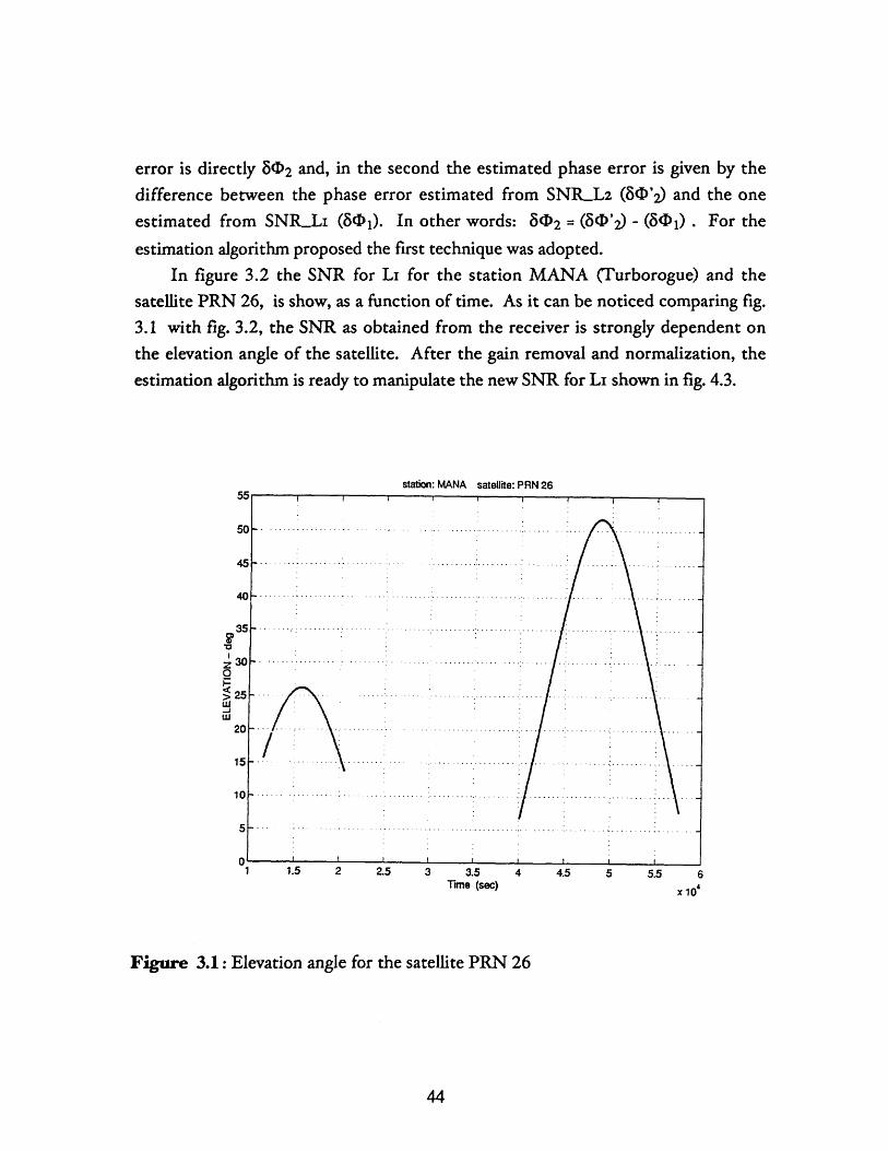
estimation algorithm proposed the first technique was adopted.In figure 3.2 the SNR for LI for the station MANA (Turborogue) and the
satellite PRN 26, is show, as a function of time. As it can be noticed comparing fig.3.1 with fig. 3.2, the SNR as obtained from the receiver is strongly dependent on
the elevation angle of the satellite. After the gain removal and normalization, the
estimation algorithm is ready to manipulate the new SNR for LI shown in fig. 4.3.
station: MANA satellite: PRN 26
1.5 2 2.5 3 3.5 4 4.5 5 5.5 6Time (sec) x 10'
Figure 3.1: Elevation angle for the satellite PRN 26

SNR Li as received by the antenna
.5 2 2.5 3 3.5 4 4.5 5 5.5
Figure 3.2: SNRILL forPRN 26.
time lsec] x 10'
the station MANA (Turborogue) and the satellite
4:00 6:00 3:00 10:00 12:00 14:00 16:00
Figure 3.3: SNRLI for the station MANA after gain correction and
normalization.
700
soo -
C400
300oo
C 200 -
100
I i l |
800
II1 1 6
7
I--

3.3.2 Data Segment Selection
After the gain correction, the SNR is divided into segments. The length of thesesegments is based on gaps that the data might have, or on the rate of change of theelevation angle, so that portions of data relevant to a rising or setting satellite aretreated separately.
The SNR might have missing data in the sequence due to problems with thereception of the signal or to obstruction of the satellite. The algorithm presents agap tolerance of about 10 epochs. If the missing data are less than 10 points, theprogram linearly interpolates before the computation of the spectra. However, thealgorithm does not interpolate when fitting the sine and cosine components,because the interpolation introduce false data which might produce a wrongestimation of the phase error. On the other hand, not having enough data for theestimation of the sine and cosine components, can cause anyway an inaccurateestimation of the phase error. If the gap is too large, separate analyses are done forthe two segments of data. Because the length of the segment of data determines thefrequency resolution, also a too short time series can lead to a wrong phase errorestimation.
3.3.3 Spectral Decomposition of the SNR
As already discussed in section 2.2.4, the scattering phenomenon is generallydue to the superposition of several single multipath contributions, each characterizedby a specific frequency fm. Multipath is not a stationary phenomenon because its
frequency varies with the rate of change of the satellite elevation angle (formula[2.5]). Therefore, spectral estimation must be performed on a span of data longenough to provide the required frequency accuracy, but short enough to allow thehypothesis of constant frequency.
The purpose of the spectral estimation performed by the algorithm is todecompose the total multipath phase error in several components and isolate themto compute the GPS phase error due to each component. The multipath
46

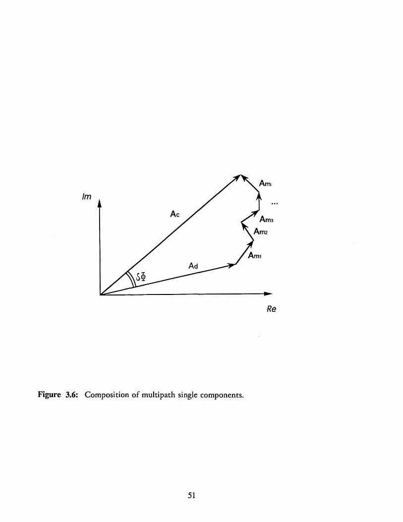
contributions are determined sequentially and the correspondent phase error arecomputed. The total phase error BQ1 EST is created from the sum of the complexcomponents of all of the contributions.
We decompose the SNR variations into individual components in an iterativeprocedure. At each iteration, we compute the power spectra of the current SNRresiduals, which in the first iteration are simply the values of the SNR after weremove the gain corrections. We select the frequency with the largest amplitude: ifthis amplitude (sqrt of the power spectral density) is larger that 1/500 of the meanSNR strength (obtained from the zero frequency component in the PDS) then theiteration is continued. The 1/500 limit is set so that the phase contribution from theremaining components will be less than 0.4 mm (190 mm/ 500).
For each period of the maximum frequency through the data segment, we estimatea mean value and sine and cosine components at this frequency. Since thefrequencies are obtained from a FFT, we are assured that there will be an integernumber of these periods in the data segment. As can be seen in fig. 3.4, forexample, the frequency of the multipath is reasonably constant but the amplitudechanges with time. Our algorithm estimates separate sine and cosine componentsfor each full wavelength through the data segmant. The sine and cosinecomponents are saved and the contribution to the SNR computed and removedfrom the SNR values. These residual SNR values are then used in the next iteration.In addition to the 1/500 amplitude limit, the iteration is continued for no more than50 iterations although this limit is rarely reached. At the end of the spectraldecomposition, we have a series of sine and cosine components, each applicable todifferent times in the data depending on the frequency they represent. For eachdata epoch, there are N applicable component pairs, where N is the number ofiterations. The compex sum of the N pairs (with their time arguments dependenton the frequency they each represent) is formed and the phase error and amplitudecomputed from the sum. The N multipath contributions estimated with thealgorithm are superimposed in figure 3.6, to provide the total multipath phase error
There are limits on the spectral components estimated. When the maximumspectral components are found, we search frequencies for 2/T to n/(2T), where T isthe total duration of the segment, and n is the number of measurements in the span.

Because the high frequency end is half of the maximum frequency in the spectrum,
the algorithm will tend to smooth the SNR as well. This smooting can be observed
in fig. 3.4.
As explained in section 2.2.2, the determination of the sign of the multipath
phase error estimate remains ambiguous. In the algorithm the sign attributed to the
multipath phase error is based on the sign of the rate of variation of the elevationangle (dO/dt). The sign actually depends on the rate of change of distance to the
reflector. Because we never try to compute the location of the reflectors, we use therate of change of the elevation angle instead. If dO/dt is positive, 86EST=-atan2(Imag,Real); if If dM/dt is negative, 8&EST=+atanz(Imag,Real). The assumption
made is that, as the satellite rises, the distance to the reflector decreases (at least for
reflections from a flat Earth). This is verified in most of the cases, but it is not true
in general. This ambiguity in the sign of the multipath phase error strongly
influences the performances of the estimation algorithm in those case when an
abrupt change of sign of the estimated phase error is observed.
The total multipath phase error estimate 8IDEsr is shown in figure 4.7 and is
indicated with LCGEST. The observed phase residual measured from the GPSmeasurements 8G0OBs is shown in the same figure (LCOBS) and compared with the
estimated phase error due to multipath. In this example, the visual correlation of the
two curves is striking: the frequency content and the amplitude of the two curves
seems to agree very well. In the following chapters, quantitative analyses (spectral and
statistical) are performed to compare estimated and observed phase residuals.

KKAU SNRL1 PRN 16 ASIA1995 6 9
4.4 4.5 4.6time (sec)
4.7 4.8
1.4
1.2
1
0.8
4.
2
1.8
1.6
1.4
1.2
4.4 4.5 4.6time (sec)
4.7 4.8
Figure 3.4: Curve fit for SNRLI satellite PRN 16. Station KKAU.
3II I
2
1.8
1 r-
................................ .................. i.....
. .. . . . . .. . . . . . . . . . .. .. . . . . . . . . . . . .. . . . .-
....
1
0.8
4.
4.9
x 10
3 4.9
x 104
SI I
I
I ,
· ·
i I
. . . . . . . . . . . . . . . . .. . . . . . . . . . . . . .. . . . . . . . . . . . . . . . . .
. . . . . . . . . . . . . . . . .. . . . . . . . . . . . . . . . . . . . . . . . .. . . . . i. . .......-. ..........................I I
KKAU SNR L2 PRN 16 ASIA 1995 6 9
4.4
4.4
4.5
4.5
4.6time (sec)
4.6time (sec)
4.7
4.7
4.8
4.8
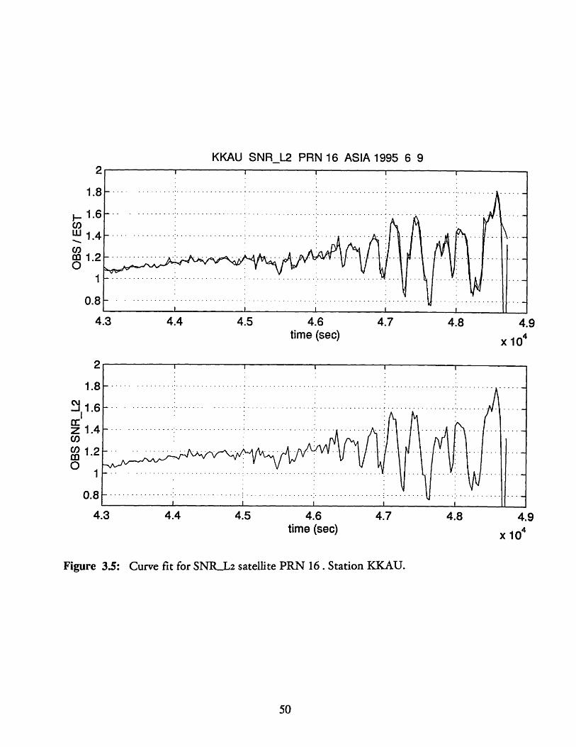
Figure 3.5: Curve fit for SNRIL2 satellite PRN 16. Station KKAU.
INI
.
2
1.8,4 I•'
1.0
1.4
1.2
1
0.8
4
2
1.8
1.6
1.4
1.2
0.8
4.
...... . . ..
F,
3I I I ~I ' I II ~ I
3
4.9
x 104
4.9
x 104
-c
3
6
. . . . .· -- - -- .' .· . .. . . . . ..
Im
Re
Composition of multipath single components.Figure 3.6:

GPS "OBSERVED" Phase Residuals for: KKAU PRN 16
4.4 4.5 4.6 4.7 4.8GPS "ESTIMATED" Phase Residuals computed from the analysis of SNR variation
0.2
0.1
0
-0.1
-0.2
4.
0.2
0.1
0
-0.1
-0.2
4.
0.2
0.1
0
-0.1
-0.2
4. 4.4
4•I
4.5 4.6Time (sec)
4.7
4.8
4.9
x 104
4.9
x o10
4.8 4.9
x 104
Figure 3 .7: The multipath phase error ( DEST = LCEST) estimated by the algorithm iscompared with the observed phase residual (60oBs =LC.OBS) computedfrom the measurements.
. ... . . I.10.. .. ... ... .. ... ... .. ... .. .. -. . . . . . . ......... - --
,............... . ................ ................ : ................ :..... v/
3
3 4.4
.................... .. . . . . ........................ ... . . . . . ... . .. ..... .. .. .. .. . .. . .
.................. ...... ...... ... .. ..
. ......... ......... ........ . ......... . ....... .
3
........ .. .. . . . . . . . . . . . . . . .. . . . . . . . . . . . . . .
................. ..........· ·--··
.
.. ... . ..
........ .... ..... .................. . ...................... ......... .....
4.5 4.6 4.7Comparison LC OBSERVED vs LC ESTIMATED
1
· '~'1
· `''~
I ....

Chapter 4
Statistical and Spectral Analysis of
estimated and observed GPS phase
errors
4.1 Introduction
The aim of the spectral and statistical analysis described in this chapter is to test
how well the retrieved multipath phase error from the Signal-to-Noise-Ratio (SNR)
agrees with the phase error observed in the GPS measurements. To this purposetwo time series, the observed phase residual (4OBs = 8sOBs) and the estimated
multipath phase error (EST = B EST), were studied and compared. This analysis
provided important information about the applicability, limits and performance of the

GPS multipath estimation method described in chapter 3. The results of this study
applied to actual GPS measurements are discussed in detail in chapter 5.
4.2 Data Preprocessing
With data preprocessing we indicate the procedure for the selection and
formatting of the GPS data before applying the analysis. The first goal of this
operation was to choose data sets containing a strong multipath error in the phaseobservable.
As mentioned in chapter 2, the occurrence of multipath produces large regular
oscillations in the SNR. However, the simple analysis of the SNR might not provide
enough information for evaluating the characteristics of the data, as ionospheric
effects can also cause wave-like patterns in the signal received by the antenna. A
discussion on the errors in the GPS phase measurements can be found in section3.2.
Because the observed phase residual, 40BS, does not contain ionospheric effects,the combined analysis of SNR and oBas gives enough information for the selection ofthe data. Whenever large structured oscillations were found in both SNR and 0oBs,
because in the observed phase residual the ionospheric effects are filtered out, wecould be confident in having GPS measurements affected by multipath, and the datawere considered appropriate for the analysis.
0oBs was computed by using the GAMIT GPS analysis software packageimplemented at MIT (King and Bock, 1993). The data chosen for this analysis wereselected by using the CVIEW option of the program.
The data sets chosen were then divided into subsections having well definedstatistical properties and multipath interference. This operation permitted us toisolate the phenomena without averaging out the effects of multipath over a largenumber of samples.

4.3 Spectral Analysis
4.3.1 Multipath frequency
The multipath phenomenon is caused by the interference of electromagneticreflections with the direct electromagnetic signal transmitted by the satellite. Thelevel and frequency of the GPS noise deriving from multipath depends upon thedistance, geometry and reflectivity of nearby objects, the elevation angle of thesatellite and the rapidity of change of the elevation angle with respect the receiver,and the value of the carrier frequency (section 2.2).
Because of the dependency of multipath on these parameters, each multipathcomponent due to a particular reflector have a distinct frequency. Therefore, themultipath noise caused by the surrounding of a receiving GPS antenna can bestudied and identified by spectral analysis (section 3.3.3).
Spectral analysis is used here to compare the estimated multipath phase error(~Esr) and the observed phase residual (oBs).
4.3.2 Power Spectral Density
In spectral analysis we try to represent a stationary process in terms of a sum ofsinusoids, in order to define its spectrum. We applied this analysis to the observedand estimated phase errors, to determine their spectral content and how this wasrelated to the multipath phenomenon.
The two time series (1 oBs j and {ESTr J, are assumed Stationary Ergodic Random
Processes. In other words, we infer that their statistical properties do not vary withtime (Stationary) and that the average values computed over the ensemble at a time
t0, 0x i (t) [ for x = OBS, EST), will equal the corresponding average values computed overtime for a single time history record, X(t)[ for x = OBS, EST} (Ergodic).
This important assumption allows us to perform our statistical and spectral analysiswithin one time series, without the need of independent realizations of the process.

Let us consider a stationary ergodic random process:
{,t} = f{(n. At)} for n = 1,2,3,...,N. [4.1]
where the time resolution interval between the sample values is At , the total number
of samples is N and the total length of data analyzed is T=N At.
The Discrete Fourier Transform (DFT) of {1j is defined as:
{)K } = {(k -Af)} = At m4(e('N• for k = 1,2,3,...,N. [4.2]
The Nyquist cutoff frequency of the sequence is f, = 1/(2 At ), and the minimum
frequency-resolution bandwidth is Af = 11T =1/N At.
Therefore, the Power Spectral Density of {1,} is given by:
2 2 [4.3]N. AAt
For each couple of time series, {OBSn)} and {ESTnrj, we computed the Power Spectral
Densities Sos , SES, and SDIFF, power spectral density of their difference {ODIFF).
Each time series was previous normalized by subtracting its mean. The DFT was
computed via FFT (Fast Fourier Transform).
The Power Spectral Density was computed by using a Matlab algorithm
(FFTobsest.diff.m) which can be found in Appendix C.
4.3.3 Auto Correlation and Cross Correlation
An other way to compare f{oBsJ and {(ESr) is to compute the Auto-Correlation of
each of the two time series (Roo and REE) and the Cross-Correlation between them
(RoE)To define Roo, REE and ROE between two time series {0OBSn) and {4 ESTn, we first
introduce the Cross-Covariance Function, CoE.

The Cross-Covariance Function between two processes I{OBsnj and {ESTr)j for anytime delay t, is given by :
COE(r)= (OoBSn -OBS)(OES(t+r) - EST (t + ')) [4.4]
If we assume again that the two time series are stationary ergodic processes, theirmeans •ROBs and grsr are constants and independent of t. Therefore, COE can be
written as:
COE( (O=BSn~ )(ESTn(t + ) OBSMEST [4.5]
We define the Cross-Correlation function between {JoBsJ and {•EST) as:
•E) = I oBSnX)(ESTn (t + r)) [4.6]
and it follows that:
COE ( = ROE()- OBSuEST [4.7]
The equivalent Auto-Covariance Functions for the time series are:
1F[4.8]
CEE()- (tES-Tn -f r S)(O Tt + -EST t(t + a)
and the Auto-Correlations for (os~s and {•--J are:

Roo (T) = [ XOBSn)(OBSn(t + )
[4.9]
RE(') = SY- (ErXrn)( ESr,(t +)
Therefore:
Coo(T)= Roo( ) -oss [4.10]CEE() = REE() 2
If the mean of either measurement is zero (p=0, = =0 or p.,=C=0 ) it follows that:
Coo(r)= Roo(r)
CEE () = REE( ) [4.11]
COE( )= ROE(r)
The Matlab program implemented for computing the Auto and Cross-Correlation
of {(OBs) and {(ESTn) is called Auto-CrossCORR.m, and is presented in Appendix
C.
4.3.4 Auto and Cross Spectral Density Function
The spectral density function between two stationary ergodic random processes
can be defined as the Discrete Fourier Transform of the Correlation function
between those records:
N 2 kn
SOE(k)= At ROEe N for k=1,2,3,...,N. [4.12]n=l
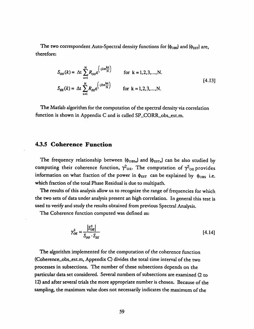
The two correspondent Auto-Spectral density functions for {oBs and {(-r}) are,
therefore:
Soo (k) = At Rooe N for k = 1,2,3,...,N.n-1
[4.13]
SE(k) = At XREe-JN) for k= 1,2,3,...,N.n-1
The Matlab algorithm for the computation of the spectral density via correlationfunction is shown in Appendix C and is called SPCORIRobs-est.m.
4.3.5 Coherence Function
The frequency relationship between {loBSn) and {IEST.) can be also studied bycomputing their coherence function, 720E. The computation of Y2 oE providesinformation on what fraction of the power in 4 EST can be explained by OBS i.e.which fraction of the total Phase Residual is due to multipath.
The results of this analysis allow us to recognize the range of frequencies for whichthe two sets of data under analysis present an high correlation. In general this test isused to verify and study the results obtained from previous Spectral Analysis.
The Coherence function computed was defined as:
2 S0E [4.14]YOE = [4.14]
The algorithm implemented for the computation of the coherence function(Coherenceobsest.m, Appendix C) divides the total time interval of the twoprocesses in subsections. The number of these subsections depends on theparticular data set considered. Several numbers of subsections are examined (2 to12) and after several trials the more appropriate number is chosen. Because of thesampling, the maximum value does not necessarily indicates the maximum of the
coherence function. The only information we can extract from the coherencefunction computed in this analysis is the range of frequencies where the two timeseries correlate better.
4.4 Statistical Analysis of GPS Phase Residuals
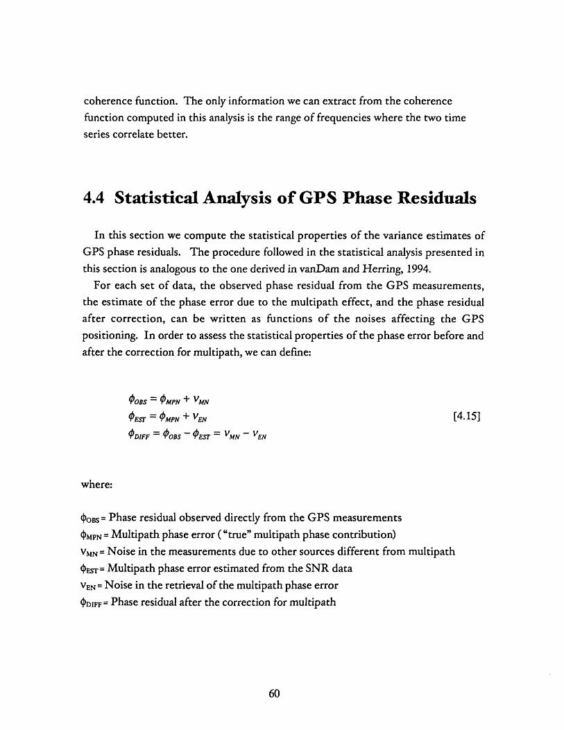
In this section we compute the statistical properties of the variance estimates ofGPS phase residuals. The procedure followed in the statistical analysis presented inthis section is analogous to the one derived in vanDam and Herring, 1994.
For each set of data, the observed phase residual from the GPS measurements,the estimate of the phase error due to the multipath effect, and the phase residualafter correction, can be written as functions of the noises affecting the GPSpositioning. In order to assess the statistical properties of the phase error before and
after the correction for multipath, we can define:
'OBS = WMPN + VMN
PEST = WMPN + VEN [4.15]ODIFF = OOBS - 'PEST = VMN - VEN
where:
OOBs = Phase residual observed directly from the GPS measurements
WMPN = Multipath phase error ("true" multipath phase contribution)
vMN = Noise in the measurements due to other sources different from multipathOEsr= Multipath phase error estimated from the SNR data
vEN = Noise in the retrieval of the multipath phase errorPDIFF = Phase residual after the correction for multipath

In this analysis it will be assumed that the time series under study are stationary
ergodic, with zero mean and standard deviation o.
Of all the quantities previously defined, only 0oBs, mEST and PDIFF are known, and
the unknown phase errors vMN, VEN and 4 MPN are assumed to be independent.
A very useful method of statistical analysis is the Chi-square test, where the Chi-
square distribution (with N-1 degrees of freedom) is given by the estimates of thevariance normalized by the expected variances. However, because OBS, EST and
PDIFF and the estimates of their variances are correlated, a simple Chi-square test
cannot be used to determine the statistical significance of the changes in the
variance estimates, due to the correction for the multipath phenomenon.
In order to perform an appropriate statistical analysis, we computed the
expectation and variance of the difference between the variance estimates of the
phase error, before and after applying the corrections for the multipath contribution.
If N is the number of samples and a the standard deviation of the time series, the
estimates of the variances of {oBs J, {4ESTn }, and {fDIFFn) are given by :
&2BS = 'V (OBSn)2 = N (VMN+MPNA 2
n=1 N-1 =i N-1
sr=$2EST L 2(0MPn+EN1) 2 [4.16]n=1 N-1 = =1 N-1
N(0 .2 MN + ENn 2&rIF n=1= N - 1 N1 N-- 1ln=l
It should be noticed that in these formulas the processes have been normalized by
subtracting their mean before computing the variances.
The expectation of the estimates of the variance can be written as:

(UE2T)1= OMpN + ENM
(&2",)= acN + al.
The expectation of the difference of the variance estimates of OOBS and DIFF iSgiven by :
(BS &D = -[4.18]
The variance of the difference in the variance estimates is :
var(BS - F) s DIFF s - FF)
If we assume that:
[4.19]
(vNolM) = 0 and (vM, vENi) =0
(OMPNiOMPNj)= ( vMN vMN) = (vENi EVj) =0 for each i j
then the variance of the difference in the variance estimates can be written as:
&2r2cS =4. qFN - 1 + 6var(OSS &DN-1 [4.20]
where oMN, aEN and (MPN are unknown, and can be retrieved by inverting the
system:
( S)= -2MN + 2PN
(sr)= oPN + o [4.21]
(&DIFF) = +U
[4.17]
for each i
Chapter 5
Applying the method of multipath
estimation to GPS data
5.1 Introduction
In this chapter we discuss the results obtained from the phase error estimationalgorithm applied to GPS measurements. In particular, three GPS data sets werechosen for this study and will be discussed in the next paragraph: the Tien-Shandata, the LIGO data and the IAP data. Among these three collections, 42 data sets,acquired between June 1995 and January 1997, were selected for multipathestimation and analysis.
Although these measurements were not originally intended for studyingmultipath effects on GPS measurements, they are suitable for testing the

performance of the method for their strong multipath contribution to the phase error
observable.
A brief description of the data sets selected, their characteristics and their
significance in this study are provided in section 5.2.
5.2 Description of the GPS stations andthe data sets analyzed
5.2.1 The Tien-Shan data
This data set was acquired during the 1995 -1996 Tien-Shan field project. The
original purpose of this campaign was to define a north-south deformation across
Tien-Shan and to study the interaction of the strike-slip faulting and thrust faulting
along the Talaso-Ferghana fault.
The two stations selected for the multipath analysis, KKAU and MANA, are part
of a network of approximately 95 sites. The network stretches across three of the
former Soviet Republics, a region extending from Uzbekistan east to the Chinese
border, and from Taldy-Kurgan (Kazakhstan) south to Tajikistan.
The station KKAU is located in Kazakhstan, at 41.695248" lat., 72.893497* long.,and 1423.2 m elevation and uses a Trimble antenna as a receiving antenna.
The station MANA was located at a seismic observatory in the town of Manas, 30
km east of Talas, in Kyrgyzstan Oat. 42.493067, long. 72.497956%, elev. 1423.2 m).
The receiving antenna is a Dome Margolin antenna.
MANA was one of three permanent sites, besides POL2 and TALG. In the fall
of 1995, the receiver was moved to a new site near the town of Talas. This was a
better location for the receiver, because it was far enough from strong reflectors and
could be more easily mantained as a continuously operating site.
These two stations were chosen for the strong multipath effect present in the
phase measurements. Every time a GPS satellite was in a particular region of the sky,

a similar clear strong multipath was observed. This fact leads to the conclusion that
large reflecting surfaces were located near the receiving antennas.
However, the different frequencies of the multipath relevant to the two stations,suggests that the reflectors were located at different distances from the receivers.
Therefore, from the comparison of the results of the statistical and spectral analysis it
was possible to gain useful information about the performance of the estimation
algorithm at different multipath frequencies and for different geometries.
KKAU and MANA use different types of antennas, Trimble and Dorne-Margolin,respectively. The performance of the algorithm for data sets acquired with differentantennas was studied.
5.2.2 The LIGO data
This data set was chosen for the particular geometry of the surroundings of the
receiver 0036 ( fig. 5.1)
A strong multipath was observed when a satellite was at about 15' elevation and 45'
azimuth. Among the LIGO measurements two data sets, relevant to the stations0028 and 0036, had the same high sampling rate (At = 5 sec). These two stations are
located at close distance from each other. As mentioned in chapter 3, the
ionospheric errors can be filtered using single differencing when dealing with short
baselines. Therefore, in this case, it is possible to treat LI and Lz separately as two
independent observables, rather than their linear combination LC.
Both estimations were performed for the dual-frequency phase residual, LC, and
for the frequencies LI and L2 individually.
5.2.3 The IAP data
This data set was acquired in January 1997, in California, during a two week fieldwork carried out as part of a course on High Accuracy GPS held at MIT. The same

measurements were repeated at the same site in two successive days, but using two
different receiving antennas: Trimble (station COSE) on January 23, 1997 and
Ashtech (station GS29) on January 24, 1997. The measurements are relevant to the
same satellites at the same time of the day, shifted by 3.5 minutes to account for the
daily change in geometry.
Moreover, the two antennas present a different gain at low elevation angles.
Because of the antennas characteristics, the multipath error is perceived differently
by the two receivers, even though the actual multipath environment is maintained
the same during the two sets of measurements.
However, it should be mentioned that the weather conditions during the second
day of measurements (performed by the Ashtech antenna) were different. On the
second day of measurements (January 24) the ground was wet, due to persistant rain.
Rain usually increases the reflection coefficient of reflecting surfaces, which can
produces an higher multipath error in the phase observable.
To study how the multipath effects can change due to weather conditions, the
estimation algorithm was tested using data acquired on two different days, one sunny
and dry, and the other gray and rainy. Comparing the measurements performed with
the same receiver in the same location under these weather conditions, yielded very
interesting results.
GPS satellite:PRN 09
ceiver
1.5m
Fig. 5.1: Geometry of the surroundings of the receiver 0036 (LIGO data).

5.3 Multipath Estimation and Results ofSpectral Analysis.
5.3.1 KKAU and MANA
5.3.1.a) KKAU (TRIMBLE 4000SSE)
The data relevant to the GPS measurements acquired by KKAU on June 10, 1995
were analyzed. Large oscillations were observed in the SNR every time a satellite
passed through a specific region in the sky (low elevation angle and 50" azimuth).
An example of this phenomenon is shown in fig. A.1.1 and A.1.2. The SNR
presents large fluctuations when the satellite PRN 16 is at an elevation 0 = 10" - 20"
and azimuth 0 = 50" - 60", at the time t=4.5 - 5.0 10 4 sec.
The observed phase error determined from the measurement, OBss, and the
multipath phase error estimated from the SNR, 4 EST, are plotted and compared in
figures A.1.4 and A.1.7. In the plots, 0oBs and OEsr are referred to as LC OBS and
LC EST, respectively. The residual phase error given by the difference of these two
phase errors, DIFF, is plotted in fig. A.1.8.a) and is called LC DIFF. The observed
phase error shows very large values in correspondence of the structured oscillations.
The amplitude of ODIFF decreases significantly after applying the correction for
multipath.
To study the characteristics and frequency content of the three time series,(observed, estimated and residual phase error) the Power Density Spectra (PSD) was
computed and plotted in fig. A.1.8.b). The PSD of OBs and 4 ESr are very consistent
for amplitude and frequency content. They exhibit three narrow distinct peaks at
frequencies between 0.001 Hz and 0.01 Hz, and one large peak at a lower frequency.
The frequency content of ODIFF is not as rich as it is for 4 0BS and OEsr.
This result suggests that the contribution due to the multipath effect is filtered out
and the remaining phase error, which does not present a clear spectral content, is
due to other sources of GPS random noise in the carrier phase observable. In this
particular case, where the multipath effect has a predominant role in the observed
phase error, the estimation algorithm and multipath filtering is efficient in reducing

the phase residual, as well as the error in the final GPS positioning. However, a low
frequency residual component is evident in the PSD of 4 DIFF. This low frequency
component might be caused by reflectors located around 1 - 2 m distance from the
antenna phase center of the receiving antenna. An other explanation for this low
frequency component could be the atmospheric refraction errors, that produce a very
similar pattern. Therefore, with only one example, it is difficult to judge if this low
frequency residual error after correction should be considered a limitation of the
performances of the estimation algorithm or just an error due to atmospheric effects.
The auto correlation functions of o0Bs and EST-r shown in fig. A.1.8.c) are very
similar and recall the auto correlation of wide-band random noise (the envelope
decreases very rapidly, with a first zero crossing at z=1/(2B), were B is the bandwidth).
The cross correlation function between 0oBs and OESr is nearly symmetrical and is
well centered at zero, again confirming the strong affinity of the two time series
being compared. Additionally, the cross-spectral density and the coherence
function of fig. A.1.8.d) corroborate this conclusion. The two time series show a very
high coherence function (about 0.8) for frequencies between 0.001 Hz and 0.01 Hz.
Another good example of how well the estimation algorithm works in presence of
strong multipath is shown in fig. in fig. A.2.1 and A.2.2. The SNR shows
distinguished oscillations whenever the satellite PRN 20 is observed by the receiver
at an elevation 0 = 10' - 24' and azimuth 0 = 40 ° - 80°, at the time t= 7.0 - 7.5 104 sec.
The observed phase error determined from the measurement, 0OBs, and the
multipath phase error estimated from the SNR, •EST, are plotted and compared in
figures A.2.3, A.2.4 and A.2.7 (segment 2.b). The residual phase error given by the
difference of the two phase errors, ODIFF, is depicted in fig. A.2.8.a).
In the PSD of 40Bs and E)sr (fig. A.2.8.b) two main peaks at the same frequencies
are predominant , but a significant difference in amplitude can be noticed.
The auto and cross correlations of fig. A.2.8.c) deserve special attention. The auto
correlation function of a random process can be directly interpreted as a measure of
how well future values can be predicted from past observations. The key information
is how large in time is the envelope of the auto correlation function. An envelope
which decays rapidly to zero as in fig. A.1.8.c) resembles the auto correlation ofwide-
band random noise. If the auto correlation decays very rapidly, the knowledge of the
exact time history from zero to time t will not significantly help us to predict future

values beyond the very near future, i.e. beyond 1/(2B) past the end of the observed
record.
A very large envelope which does not decay rapidly, but which remains almost
constant over the near future (central peak 1/(2B) ), as in fig. A.2.8.c), resembles the
auto correlation of a sin/cos wave + random noise. This suggests that it is possible to
predict future values of the data, based on past observations, assuming that the data
remain stationary. This comparison of the auto correlations of the two time series
with the auto correlations of functions equal to the sum of a sinusoid and random
noise, confirms the influence on o0ss and 4~E of the multipath (sinusoidal in shape)
and of the contributions due to other GPS noises (random noise).
Auto and cross spectral power density and high values of the coherence function
(fig. A.2.8 d)), confirm the strong affinity of estimated multipath phase error and
observed phase error. As will be discussed in section 6.4, the multipath estimation
algorithm is very effective when multipath is the main source of phase error in the
GPS measurements, as for the receiver-satellite pair KKAU-PRN 20, segment 2.b.
This is confirmed by another interesting example relevant to KKAU -PRN 22,
segment #1. The SNR (fig. A.3.2) presents an evident sinusoidal pattern when
the satellite PRN 22 is at an elevation 0 = 100 - 30' and azimuth 4 = 50", at t=0.0 - 5.0
103 sec. The observed phase error determined from the measurement and the
multipath phase error estimated from the SNR are presented in figures A.3.3 and
A.3.4. The residual phase error 4 DIFF is plotted in fig. A.3.5.a). For the Power
Spectral Density (fig. A.3.5.b)), the auto and cross correlation (fig. A.3.5.c)), the auto
and cross spectral density and the coherence function (fig. A.3.5.d)) were
computed. Analogous observations than those for KKAU-PRN 20 can be applied.
The examples reported so far are relevant to cases in which a strong, clear
multipath phenomenon at frequencies between 0.001 Hz and 0.01 Hz is observed in
the phase residual. In these cases the estimation algorithm showed good
performances, as determined by spectral analysis. But how does the estimation
algorithm work in the presence of other sources of noise or in the presence of a
lower frequency multipath? To answer this question segment #2 of the data set
relevant to KKAU-PRN 22 was studied. In fig. A.3.6 the observed phase error
shows a low frequency component which is not present in the phase error estimated
from the SNR. As discussed above, this low frequency undulation might be caused

by multipath due to close reflectors or by atmospheric refraction. In fig. A.3.7 a)4 DIFF presents a large amplitude, and a low frequency component.
The PSD of fig. A.3.7b) shows the very different frequency content of the
observed and estimated phase error. In fig. A.3.7.c) the two auto correlation
functions show very different properties, and the correlation between the two series
presents low amplitude and evident asymmetry with respect to the zero. A very low
coherence function is found in fig. A.3.7.d) for all the frequency spectra.
5.3. .b) MANA (ROGUE SNR-8000)
When the SNR data relevant to the measurements acquired by MANA on June
10, 1995 were analyzed, large oscillations were observed every time a satellite was
found at low elevation angle and about 300" azimuth.
It appears evident in fig. A.4.1 and A.4.2 that the SNR exhibits large fluctuations
when the satellite PRN 26 is at 0 = 18" - 22* and 0 = 250* - 320', at t=1.0 - 2.0 104
sec. 0oBs and OEST are shown in figures A.4.3 and A.4.4. #DIFF, is plotted in fig.
A.4.5.a). Even though the large oscillations of 4oas are well matched by OESr, the
frequency content of the two time series is quite different. OBss presents a broader
spectra (Af=0.0003 - 0.003 Hz), while OEsr has a sharp peak at about 0.0015 Hz,
therefore a frequency component at 0.00085 Hz is still present in ODIFF, as shown in
fig A.4.5.b).
The auto and cross correlations are shown in fig. A.4.5.c). The coherence function
(fig. A.4.5.d) is about 0.6 in the interval of frequency between 0.001 and 0.01 Hz.
Large oscillations of the SNR were also observed for PRN 28 (fig. A.5.2) when the
satellite was at an elevation 0 = 15" - 35" and azimuth 0 = 250" - 310", at t=4.5 - 5.3 104
sec (fig. A.5.1). OoBs and OESr are presented in figures A.5.3 and A.5.8. ODIFF is
depicted in fig. A.5.9.a). Even though the statistical analysis shows a very strong
decrease of the phase error after the correction for multipath, the frequency content
of Ooss and OEST is quite different, and a large lower frequency component is found in
vDIFF, as observed in fig. A.5.9.b).

The auto and cross correlations of fig. A.5.9.c) suggest a predominance of random
noise on the multipath effect in the phase error. The coherence function (fig.
A.5.9.d) is close to 0.7 in the interval of frequency between 0.001 and 0.01 Hz.
5.3.1.c) Discussion and Comparison
The previous analysis shows that the multipath frequency for KKAU is usually
higher than the one observed for MANA.
In figures A.1.8.b) , A.2.8.b) and A.3.5.b) it is evident that the multipath
frequency for KKAU is usually in the range 0.002-0.004 Hz.
For MANA, the multipath frequency is lower than for KKAU and it is in the range
0.0009 - 0.0010 Hz. This indicates that the reflecting surface producing the
multipath in this case (MANA) is closer to the receiving antenna and its effect is
also more intense. The relationship between the distance of the reflector and the
multipath frequency is given in [2.17].
5.3.2 Stations 0036 and 0028 (TRIMBLE 4000SSE)
5.3.2.a) 0036: Dual-band processing
Some a priori information relevant to this site were available and were used to
better interpret the results of the spectral and statistical analyses. The geometry of
the surroundings of the receiver 0036 is depicted in figure 5.1, where the incoming
signal from the satellite PRN 09, located at about 15" elevation and 45' azimuth,reaches the receiver after multiple reflections. The SNR relevant to this satellite-
receiver pair is plotted in fig. A.6.4. The SNR is affected by very distinct largeoscillations when the satellite is at an elevation 0 = 14" - 22* and azimuth < = 40* - 50",
at t=7.3 - 7.5 104 sec (fig. A.6.3).

OBs and OEsr are compared in figures A.6.5 and A.6.6. The difference between
the two phase errors is plotted in fig. A.6.7.a).
The PSD of 0oBs and OEsr (fig. A.6.7.b) exhibit one narrow distinct peak at about
0.001 Hz. This information suggests that in this case the multipath is not produced
by a complex scattering from several reflectors, but from one distinct reflector
producing one distinct frequency component.
Because of the coherence of the two time series, the frequency content of ODIFF
does not present any strong predominant frequencies. This implies that the main
contribution to the phase error is due to multipath and is filtered out by the
correction. The remaining phase error is due to the other sources of GPS random
noise, which cannot be corrected with this method.
The auto correlation functions of 0oBs and OEST shown in fig. A.6.7.c) present very
interesting patterns. The envelope amplitude diminishes slowly and recalls the auto
correlation of a narrow-band random noise, where the first zero crossing is at t=1/B
(B is assumed small). The bandwidth is smaller in EsTr, causing its auto correlation
function to decay slower than the auto correlation of OoBs. It can be concluded that
Oos contains more random noise and a larger bandwidth scattering.
The cross-spectral density and the coherence function of fig. A.6.7.d) reinforce
the conclusion that a distinct frequency is dominant in the signal, with very narrow
bandwidth. The two time series show a high coherence function (about 0.7) for
frequencies between 0.001 Hz and 0.01 Hz.
Another example of strong multipath is shown in fig. A.8.5 and A.8.6. The SNR
relevant to the satellite PRN 25 shows large oscillations when the satellite was at an
elevation 0 = 15' - 20' and azimuth 4 = 164' - 168', at t= 7.5 - 7.7 104 sec. The
observed phase error determined from the measurement and the multipath phase
error estimated from the SNR are plotted and compared in figure A.8.7 (segment
#1). oDIFF is shown in fig. A.8.8.a). In this case the oscillations are not as distinct as
for PRN 09.
The PSD of 0oBs (fig. A.8.8.b) show two narrow peaks, respectively, at frequencies
of 0.001 Hz and 0.002 Hz. OEsr presents a narrow main peak at 0.002 Hz and a broad
band low frequency peak between 0.0001 Hz and 0.0005 Hz. As a result of this
spectral difference, the PSD of ODIFF has a predominant low frequency spectral
content.

The auto and cross correlations of fig. A.8.8.c) present an envelope rapidlydecreasing to zero, as for wide band random noise. This suggests that the multiplephase error does not come from a single reflector, as in the previous case for PRN09, but might be due to a more complex scattering phenomenon from close anddistant surfaces. The cross-spectral density and the coherence function of fig.A.8.8.d) reinforce this conclusion. The two time series show a coherence functionof about 0.6 for frequencies between 0.001 Hz and 0.01 Hz.
An interesting example where there is a noticeble difference of amplitudebetween 4os and 4 EST, rather than of frequency content, is given by LIGO 0036,PRN 15. (segment #4). ODIFF is computed in fig. A.7.10.a). The observed phase
residual presents small oscillations similar to the ones found in the estimated phaseerror, but with a different amplitude: 0oss is always negative while ESTr is shiftedupward and presents some positive and negative values.
The Power Spectra Density (PSD) of this segment of data is shown in fig.A.7.10.b). The PSD of OBs and EsrT are consistent at high frequencies. They bothexhibit one peak close to 0.001 Hz.
The auto correlation functions in fig. A.7.10.c) are very different and the crosscorrelation is asymmetric and small in amplitude.
5.3.2.b) 0036 and 0028: Single Differences for short-baseline LI and L2
As discussed above, for short baselines the ionospheric effects can be filteredusing single differencing. In this case it is possible to study the effect of multipathat each of the two GPS frequencies and the performance of the estimation algorithmfor LI and L2.
In this section we show the results of the analysis of LI and Lz separately, as twoindependent observables. l1OBS, slEST, and 4 1DIFF indicate respectively, the
observed phase residual, the multipath phase error and their difference, respectively,for LI.
OloBs and IlEST are compared in fig. A.9.1 and A.9 2. I1DIFF is shown in fig.A.9.3.a). PSD of loBs and O'EST are presented in fig. A.9.3.b).

The spectral content of 01OBs and $IEST is very similar at higher frequencies,showing a predominant peak at 0.002 Hz, but does not agree at lower frequencies.Therefore, the PSD of OIDIFF shows a spectral content only at lower frequencies(below 0.001 Hz).
The auto correlation of ~'EST (fig. A.9.3.c) recalls the one of a narrow-bandrandom noise. The cross correlation Roe is well centered but slightly asymmetric. Agood coherence is found at f=0.001 Hz.-0.01 Hz (fig. A.9.3.d). In this case thefrequency content matches very well, but the shift in amplitude causes (1DIFF tO staylarge also after the correction. A very different result is obtained for L2 (fig. A.9.4and A.9 5), where the amplitude of 02DIFF is well reduced (fig. A.9.6.b) ), eventhough a low coherence is observed (fig. A.9.6.d) ).
5.3.3 COSE and GS29
5.3.3.a) COSE (TRIMBLE 4000SSE)
The data considered for this analysis were acquired on January 23, 1997 using aTrimble antenna . Any time a satellite was at a low elevation angle ( 0 = 10" - 20" )and azimuth 0 = 50' - 70", the SNR showed large oscillations at LI and L2. Anexample of the multipath phenomenon occurring in proximity of COSE is providedin fig. A.11.1 and A.11.2.
The satellite PRN 25 passed through the critical region in the field of view ofCOSE at t=5.6 - 6.2 104 sec. OBas and ES~rare plotted and compared in figure A. 11.3(segment #3). ODIFF iS computed in fig. A.11.6.a).
The observed phase error presents only one very large oscillation at the end of thesegment, probably due to reflections from the ground because the antenna waslocated on a large slope. The satellite was setting and this strong reflection cantherefore take place at a very low elevation angle (0 = 10").
The Power Spectral Density of this segment of data is shown in fig. A.11.6.b).The PSD of 4OBs and OEST are very consistent for amplitude and frequency content.
They both exhibit large peaks at the same frequency, about 0.001 Hz, but with verydifferent amplitudes. This is the reason why ODIFF still carries a considerable
frequency content. In this particular case, it is not the frequency content, but the
amplitude of the multipath phase error estimated by the algorithm that produced the
critical result. An overestimation of the amplitude of the oscillation increases the
total phase error after the multipath correction.The auto correlation functions of Oos and EST shown in fig. A.11.6.c) recall the
auto correlation of a wide-band random noise. The cross-spectral density of fig.A.11.8.d) confirm the previous results of the spectral analysis. The two time seriesshow a very high coherence function (about 0.8) for frequencies between 0.0005 Hzand 0.01 Hz.
An interesting case to study is COSE PRN 01, segment lb., In chapter 3 thetechnique for the multipath estimation was described. When the fit of the multipathmodel and the SNR curve is performed, some problems can rise, due to the methodused for the fit (section 3.3.3). ODIFF presents sudden changes of sign deriving from
mESr (fig. A.9.6.a)). Correlation and spectral analysis show a poor agreement between
O0sS and OEsr.
5.3.3.b) GS29 (ASHTECH Z-XII3)
The same set of GPS measurements discussed in section 5.3.3.a) were repeatedby using an Ashtech antenna, placed at the same location of COSE, the day after (onJanuary 24, 1997). As for COSE, the satellite PRN 25 was considered, and the
analysis on the station GS29 was performed (fig. A.14.1 and A.14.2 )
O0Bs and OEsr are shown in figure A.14.3 and A.14.4 (segment #3). ODIFF iscomputed in fig. A.14.7.a). The observed phase error presents only one very large
oscillation at the end of the segment, as was observed for COSE.The PSD of this segment of data is shown in fig. A.14.7.b). The PSD of o0s and
mEST are very consistent for amplitude and frequency content. They both exhibit onelarge peak of similar amplitude at about 0.001 Hz. DIFF does not present a
considerable frequency content, because in this case the frequency content and the

amplitude of the multipath phase error estimated by the algorithm match very well
the observed phase error. Therefore, as will be discussed in the statistical analysis,the application of the algorithm produces a strong decrease of the phase error afterthe multipath correction.
The auto correlation functions of 04s and Omr presented in fig. A.14.7.c) is
similar to those found for wide-band random noise. The cross-spectral density of fig.A.14.7.d) confirms the previous results of the spectral analysis. The two time seriesshow a very high coherence function (about 0.8) for frequencies close to 0.002 Hz.
In the conclusion of section 5.3.3.a) and 5.3.3.b), it was found that the estimationalgorithm applied to data acquired at the same location and the same time of the daywith two different antennas presented different performances. The algorithm seemsto work better for Ashtech antennas. However, because the weather conditionsduring the two successive days were not the same, it is difficult to assess if the resultsare actually due to the antenna type, or to the higher multipath effect observed on rainydays. We already noticed that the multipath estimation algorithm is very efficientwhen strong multipath is observed, especially if it is predominant with respect to otherkinds of noise. It is therefore possible that a different wetness of the ground,producing a higher reflectivity of the reflecting surfaces, might have caused a better
performance of the algorithm. One way to answer this question is to consider two sets
of measurements acquired with the same antenna, during these two days of
observations and compare the results. This is done in the next section, forCOSO(Ashtech).
5.3.3.c) COSO (ASHTECH Z-XII3)
For this analysis we selected the measurements relevant to the satellite PRN 30,because of the large oscillations observed in SNR and 0oBs (fig. A.15.1 and A.15.2).The phase residual DIFF is shown in fig. A.15.3.a). The PSD of o0Bs and rESr (fig.A.15.3.b) ) present the same peaks at 0.0005 Hz, but 90Bs also has peaks at lower
and higher frequencies (0.0001 and 0.001), which are found again in the PSD of
'DIFF.

The correlation of the two series (fig. A.15.3.c) ) as well as the coherence (fig.
A.15.3.d) ) is very poor.
The same measurement was repeated the next day, in weather conditions favorable
for strong multipath (rainy day). The phase residuals relevant to these measurements
are plotted in fig. A.16.1 and A.16.2. The PSD of 0 Bs and 4ESr (fig. A.16.3.b) )
present a very similar spectral content, showing a predominant peak at 0.0004 Hz.
The correlation (fig. A.16.3.c) ) and coherence (fig. A.16.3.d) ) are higher than in
figures A.16.3.c) ) and (fig. A.16.3.d) ). This result confirms that the wetness of the
ground increases the multipath effects, and therefore the performance of the
estimation algorithm improves.
5.4 Multipath Estimation and Results of theStatistical Analysis
The following is a summary of the results obtained from the statistical analysis of
the GPS phase residuals, described in Chapter 4. The study focused on 6 GPS
stations, MANA, KKAU, 0028, 0036, COSE and GS29, because of their strong
multipath environment. The analysis includes 42 sets of data, collected and sorted
in tables B.1.a) and b) through B.5.a) and b).
The variance of the observed phase residual is referred to as GOBS 2 , and denotes
the total phase error due to the combined effects of different sources of noise for
the GPS carrier phase observable. ausr 2 is the variance of the estimate of the
multipath phase error retrieved by using the SNR information. The difference
between oBs 2 and GOr 2 is the corrected phase error, and its variance is denoted
with ODIFF2 . The difference of variance of the phase error before and after the
correction for multipath was computed along with the statistical uncertainty of the
estimate of the change. This computation allows us to determine how well the
correction improves the GPS positioning by quantitative means.
Whenever a negative value is obtained for (GooBs 2 - GDInr2), the correction for the
multipath phase error does not reduce the variance of the total phase error. Apositive value, on the other hand, would imply a decrease of the variance of the GPS
phase error, and, thus, an improvement in the final GPS positioning. When such apositive value is obtained, the percentage decrease of variance was computed, tomake it easier to quantify the improvement of the variance after correction.
There is a noticeable decrease of the variance after the multipath correction anytime the variance of the "true" multipath noise oMPN 2 is higher or at least comparableto the variance of the GPS measurement noise, oMN2, due to other sources of noise
different from multipath. In other words, the algorithm for multipath phase errorestimation shows very good performance whenever the multipath effect is the mainsource of phase error. Good examples of this observation are given in MANA 26 lband MANA 28 2a (Table B.l.a and b), KKAU 16 2c (Table B.2.a and b), LIGO0028-0038 09 1 (Table B.3.a and b) and GS29 25 3 (Table B.5.a and b). In thesecases the decrease of variance of the phase error after correction is more than 35%.
The value yEN 2 is a measure of the error due to the estimation process and gives
information about the accuracy of the procedure for the phase error estimation.The examples previously discussed present a small GEN2 value with respect to the
multipath noise variance oMPN2. This result confirms that the estimation algorithm is
most accurate when a strong multipath is present.However, an exception to the previous cases is COSE 01 ic (Table B.4.a and b), a
measurement performed with a Trimble antenna. Even though the multipath noisevariance is more than 3 times larger than aMN 2, the multipath estimation noise is ofthe same order of magnitude as oMPN 2 and the decrease of variance after correction
is only 4%. This measurement was repeated the following day , in rainy weather,exactly at the same location, using an Ashtech antenna (GS29 01). It turns out thatOMN2 drops to 1/10 the value of ouCPN 2 and the decrease of variance after correction
improves to 16 % (Table B.5.a and b).Good examples of poor multipath in an otherwise very noisy measurement
( oMPN2 << MN 2 ) are MANA 26 2c (Table B.l.a and b) , KKAU 22 2 (Table B.2.a
and b) and GS29 25 1 (Table B.5.a and b). In these cases there is no decrease ofvariance after correction and the estimation noise variance aEN2 is larger than themultipath noise variance ouPN2 itself.

Chapter 6
Conclusions
The algorithm for the estimation of the GPS multipath phase error presented in
this thesis was applied and analyzed, to test its performance and limits. The
estimated multipath phase error and the observed phase residual were compared by
spectral and statistical analysis.
In most of the cases analyzed, a broad-band coherence function between the
observed phase error and the estimated multipath phase error was found in presence
of strong multipath. This suggests that the effects of multiple reflectors are correctly
estimated by the proposed algorithm. In other words the technique of estimating
each multipath phase error iteratively from the spectral analysis of the SNR and of
adding each contribution to obtain the composite value, produces a correct
estimation of the total multipath phase error.
In particular, the set of data which show the highest coherence (MANA and
KKAU and LIGO 0036) have multipath frequencies between 0.001 and 0.01 Hz.
Because the multipath frequency depends on the distance of the receiving antenna
from the reflecting surface, knowing the elevation angle of the satellite and its
variation with time, we can derive the distance of the reflecting object. The spectral
analysis suggests that the estimation algorithm presents good performances for
reflectors located at distances between 5.50 m and 55.0 m from the receiving

antenna, for an elevation angle of 10* and a rate of change of the elevation angle of
0.1 mrad/sec. The high coherence is confirmed by the statistical analysis, which
shows a significant decrease of the RMS of the phase residual after the multipath
correction.
When the multipath effect is due to reflections from the ground (about 1.5 - 2.0
m) the multipath frequencies are lower (COSE and GS29). At lower frequencies it
was found that the algorithm performed better for data sets acquired in the same
location by an Ashtech receiver (GS29, January 24,1997), rather than a Trimble
(COSE, January 23,1997). This result can be due to the different receiver types, the
different antenna gains or/and the weather conditions.
As explained in section 2.3, Trimble and Ashtech receivers use different
techniques for the signal processing of L2 in presence of antispoofing. Trimble
receivers cross correlate L2 with LI and the available SNR limits the bandwidth of
the L2 carrier. A narrower bandwidth corresponds to a longer integration time,which makes it more difficult to track large oscillations of the SNR, especially at low
frequencies. Ashtech receivers use the Z-tracking technique, which provides a
better SNR compared to other techniques. Because the estimation algorithm
proposed in this thesis manipulates the SNR information to retrieve the multipath
phase error, the errors introduced by each receiver in the determination of the SNR
strongly influence the performance of the algorithm.
GPS measurements acquired by the station COSO in the same days, one sunny
and dry (January, 23 1997), the other rainy and gray Ganuary, 24 1997), suggests that
also the weather conditions considerably change the performance of the algorithm.
A higher water content in the ground increases its reflection coefficient, causing the
multipath effects to be stronger in rainy more than in dry weather. On the other
hand, the performance of the algorithm is good when strong multipath is observed,because the main contribution to the observed phase residual is due to the multipath
phase error. In other words, when multipath is the main error contribution, the
estimated multipath phase error is highly correlated to the total observed phase
residual.
Low frequency oscillations of the SNR might also be produced by the ionosphere
(scintillation) but these effects are likely to be small. Low frequency SNR variations
are most likely to be due to the gain pattern of the antenna, especially for the

Trimble antennas. These antennas are known to have azimuthally dependent gainpatterns, which are not accounted for in the estimation algorithm. The algorithmmight interpret these oscillations as multipath, and, therefore, estimate a false phaseerror.
We already pointed out that different antennas might influence the performancesof the algorithm. The Dorne-Margolin antennas have a higher gain pattern at verylow elevation angles with respect Trimble antennas: this suggests that moremultipath contributions from lower elevation angles are received with a higheramplitude.
The study of short baselines (LIGO 0036-0028, PRN 09) allows as to consider thesingle differences for LI and L2 separately: the results of the spectral analysis show ahigh broad-band coherence for the multipath phase error at LI but a very lowcoherence at L2. However, in both cases the multipath estimation produces adecrease of the RMS of the total phase error after correction, as it is shown by theresults of the statistical analysis. The best performance in terms of both, spectraland statistical analysis was obtained using the estimation algorithm for the dual-frequency mode (LCEST). Because the square root of the PSD (power spectraldensity) of the observed phase error is almost equal to the sum of the square root ofthe estimated phase error and the difference between observed and estimated forthe most of the cases, we can deduce that the two curves we are comparing(LCLOBS and LC_EST) are in phase, and there is only a difference in amplitudebetween them. This is consistent with having a very high correlation function andwith L2 having the correct phase but the wrong amplitude.
One problem of the estimation algorithm which is important to mention is relatedto the sign of the phase error. As it was pointed out in chapter 2, the same SNR canbe due to opposite values of the phase error, (positive and negative). Therefore, thesign of the phase error cannot be uniquely determined. In some cases thisindetermination might cause an abrupt change of the sign of the estimated phaseerror (COSE PRN 01, segment lb), producing a considerable degradation of theperformances of the estimation procedure.
In summary, the proposed algorithm shows good results when multipath is themain contribution to the total phase error and it frequency is in the range 0.001-0.01Hz. At lower frequencies, the performance depends on the receiver-antenna type

and the weather conditions. The sign of the phase error and the nature of the lowfrequency oscillations are critical for the results of the estimation.

References
Axelrad, P., C. J. Comp and P. F. MacDoran, "Use of Signal-to-noise Ratio for
Multipath Error: Correction in GPS Differential Phase Measurements:
Metodology and Experimental Results", Proceedings of ION GPS-94,
September 1994.
Balanis, C.A., 1982, Antenna theory: analysis and design. New York: Harper and
Row series in electrical engineering.
Balanis, C.A., 1989, Advanced Engineering Electromagnetics, John Wiley & Sons
Becker, D., P. Hartl and K.-H. Thiel, A special method of managing multipath
effects,
Bendat, J.S. and A.G. Piersal, Engineering Applications of Correlation and Spectral
Analysis, John Wiley&Sons, Inc., 1993.
Bletzacker, F. " Reduction of Multipath Contamination in a Geodetic GPS
Receiver," Proceedings of the First International Symposium on Precise
Positioning with the Global Positioning System, U.S., Department of Commerce,
National Oceanic and Atmispheric Administration, Rockville, MD, pp. 413-422,
April 1985.

Blewitt, G., "Advances in Global Positioning System Technology for Geodynamic
Investigations: 1978-1992" in Contributions of Space Geodesy to Geodynamics:
Technology, Geodyn. Ser., Vol.25, edited by D.E. Smith and D.L. Turdotte,
pp.195-213, AGU, Washington, DC, 1993.
Blewitt, G., "Carrier Phase Ambiguity Resolution for the Global Positioning System
Applied to Geodetic Baselines up to 2000 km", Journal of Geophysical
Research, Vol. 94, No. B8, pp 10187-10203, August io, 1989.
Bock, Y., Gourevitch, S.A., Counselman III C.C., King R. W., and Abbot R.I., "
Interferometric analysis of GPS phase observations, Manus. Geod., II, 282-288,
1986.
Braasch, M., " On the Characterization of Multipath in Satellite-Based Precision
Approach and Landing Systems", Ph.D. Dissertation, Deparment of Eleectrical
Engineering and Computer Engineering, Ohio University, Athens, OH, June
1992.
Braasch, M., "Isolation of GPS Multipath and Receiver Tracking Errors,"
Proceedings of the ION National Technical Meeting, San Diego, CA, Institute
of Navigation, Washington, DC, pp. 511-521, Jan. 1994.
Breeuwer, E., "Modeling and Measuring GPS Multipath Effects," Master's Thesis,
Department od Electrical Engineering, Delft University of Technology, Delft,
The Netherlands, January 1992.
Clark, T., "GPS antennas: De-mystivying Multipath", NASA Goddard International
Memorandum, March 5, 1992.
Collin, R.E., Zucker F.J., Antenna Theory, McGraw-Hill, 1969.
Counselman, C., and Gourevitch, S., "Miniature Interferometer Terminals for Earth
Surveying: Anbiguity and Multipath with Global Positioning System," IEEE
Transaction on Geoscience and Remote Sensing, Vol. GE-I9, No.4, pp. 244-252,
I98I.
Counselman, C., "Miniature Interferometer Terminals for Earth Surveying (MITES):
Geodetic Results and Multipath Effects," Digest of the International
Geoscience and Remote Sensing Symposium, Washington, DC, Institute of
Electrical and Electronics Engineers, New York, pp 219-224, June 1981.
Dong, D., Bock Y., " Global Positioning System Network Analysis With Phase
Ambiguity Resolution Applied to Crustal Deformation Studies in California.
Elosegui, P., J. L. Davis, R. T. K. Jaldehag, J. M. Johansson, A. E. Niell and I. I.
Shapiro, "Geodesy using Global Positioning Systems: The effects of signal
scattering on estimates of site position", Journal of Geophysical Research, Vol.
Ioo, No. B7 , pp. 9921-9934, 1995.
Evans, A., "Comparison of GPS pseudorange and Biased Doppler Range
Measurements to Demonstrate Signal Multipath Effects," Proceedings of the
International Telemetering Conference, Las Vegas, NV, Instrument Society of
America, Research triangle Park, NC, pp.795-8 01, Oct. 1986
Georgiadou, Y. and Kleusberg, A., "On Carrier Signal Multipath Effects in Relative
GPS Positioning" Manuscritpa Geodetica, Vol.i3, pp. 172-179, 1988.
Hajj, G. A., The Multipath Simulator: A Tool Toward Controlling Multipath, in
Proceedings of the 2nd Symposium on GPS Applications in Space, Hanscom
AFB, MA, 1990.
Herring, T.A., "Precision of Vertical Position Estimates from Very Long Baseline
Interferometry", Journal of Geophysical Research, Vol. 91, 9177-9182, 1986.
Herring, T.A., "Precision and Accuracy in Intercontinental Distance
Determinations Using Radio Interferometry", Ph.D. Dissertation, Department of
Earth and Planeraty Sciences, at the Massachussets Institute of Technology, July,
1983.
King, R.W., and Y. Block, Documentation for the MIT GPS analysis software:
GAMIT, Mass. Inst. of Technology, Cambridge, 1993.
Kong, J.A., Electromagnetic Wave Theory, John Wiley & Sons, 1990.
Kee, C. and B. W. parkinson, Calibration of Multipath Errors on GPS Pseudorange
Measurments,
Kraus, J.D., "Electromagnetics", McGraw-Hill Inc., 1992.
Meehan, T., and Young, L., "On-Receiver Signal Processing for GPS Multipath
Reduction," Proceedings of the 6th International Geodetic Symposium on
Satellite Positioning, Columbus, OH, Defense Mapping Agency and the Ohio
State University, Columbus, OH, pp. 200-208, March 1992.
Oppenheim, A.V., R.W. Schafer, Discrete-Time Signal Processing, Prentice-Hall
Inc., Englewood Cliffs, NewJersey 07632, 1989.
Parkinson, B., Spilker Jr, J., "Global Positioning System: Theory and Applications,"
Vol.I and Vol. II, Volume 163 and Volume 164, Progress in Astronautics and
Aeronautics, Published by the American Institute of Astronautics and
Aeronautics, Inc. 370 L"Enfant Promenade, SW, Washington, DC 20024-2518.
Schupler, B. R. and R. L. Allshouse, "Signal Characteristics of GPS User Antennas",
Navigation: Journal of the Institute of Navigation, VoL 41, No.3, pp 277-295, 1994.
Schupler, B. R., R. L. Allshouse and T. A. Clark, Signal Characteristics of GPS User
Antennas, Navigation, Vol. 41, 277-295, 1994.
Sennott, J., and Pietraszewski, d., "Experimental Measurements and
Characterization of Ionospheric and Multipath Errors in Differential
GPS,"Navigation, Vol. 34, No.2, pp.160-173, 1987.

Spilker, J.J., "GPS Signal Structure and Performance Characteristics", J. of Inst.
Navig., VoL 25(2), pp. 121-146, 1978.
Tranquilla, J., and Carr, J., "GPS Multipath Field Observations at Land and Water
Sites", Navigation, Vol. 37, No.4, pp.393-414, 1991.
Tranquilla, J.M., Carr, J.P., Al Rizzo, H.M., "Analysis of a Choke ring groundplane
for multipath control in Global Positioning System (GPS) applications" , IEEE
Trans. Antennas Propag., Vol. 42, pp 905-911, 1994.
Van Dam, T.M., T.A. Herring, "Detection of atmospheric pressure loading using
very long baseline interferometry measurments", Journal of Geophysical
Research, Vol. 99, No. B3, pp. 4505-4517, March io, 1994.
Van Nee, R., "Multipath Effects on GPS Code Phase Measurements," Proceedings
of ION GPS-9I, Albuquerque, NM, Institute of Navigation, Eashington, DC,
Sept. 1991, pp. 915-924.
Van Nee, R., "Spread Spectrum Code and Carrier Synchronization Errors Caused by
Multipath and Interference," IEEE Transactions on Aerospace and Electronic
Systems, Vol. 29, No. 4, PP- 1359-1365, 1993.
White, P.H., "Cross-Correlation In Structural Systems: Dispersive ans Non-
Dispersive Waves", Journal of the Acoustic Society of America, Vol. 45, No. 5, pp.
1118, May 1969.
Young, L.E., Neilan R.E., and F.R. Bletzacher, "GPS Satellite Multipath: An
Experimental Investigation" Proceedings of the First Symposium on Precise
Positioning With the Global Positioning System, National Oceanic and
Atmospheric Administration, Rockville, Maryland, pp.423-432, 1985.


Appendix A
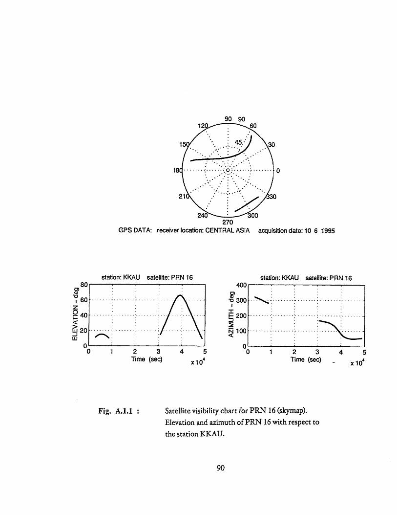
90 9060
. ., 30
21
240 300270
GPS DATA: receiver location: CENTRAL ASIA acquisition date: 10 6 1995
station: KKAU satellite: PRN 16
Time (sec)
Fig. A.1.1 :
40C
30C
200
100
0
station: KKAU satellite: PRN 16
I·I, - , !
0
x 104
1 2 3 4 5Time (sec)
Satellite visibility chart for PRN 16 (skymap).Elevation and azimuth of PRN 16 with respect tothe station KKAU.
90
1
x 10'
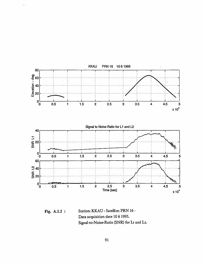
KKAU PRN 16 10 6 1995
0 0.5 1 1.5 2 2.5 3 3.5 4 4.5 5x 10
Signal to Noise Ratio for L1 and L2
0.5 1 1.5 2 2.5 3 3.5 4 4.5 5
0 0.5 1 1.5 2 2.5 3 3.5 4 4.5 5Time (sec) v n4
Fig. A.1.2 : Station: KKAU - Satellite: PRN 16 -Data acquisition date 10 6 1995.
Signal-to-Noise-Ratio (SNR) for Li and L2.
80
-c60
o40
_ 20Uj
g I I I I
20
_I · · · ·
I
I ·
· ·
I r I
........ ..--- · ·----.-
1 I
I I I I I I I I I.. ...·........ .·..... ·.........·... -! .·.... ~ .......~t I | |
,. . .
I
A III,

GPS "OBSERVED" Phase Residuals for: KKAU PRN 16 - ASIA 1995 6 10
I- I
| ... I .• : :-.... . .... -..'- ' ." ""_. ........ ....... ......... !. ...... ...• ii•' :I .. .. i ........ ....... .. ..- ; ..-... .: ::. ...... ., .. . ... ..... ..... ...... .... .: .- -.. .
." ..." ."1" .. . .. . ." ......... ........... ........... .........•; ·
I " I·-- · ·- · · ·I · · · ·-- · ·: I I ..-
0 0.5 1 1.5 2 2.5 3 3.5 4 4.5 5GPS "ESTIMATED" Phase Residuals computed from the analysis of SNR variation x10
........... ....................... . ... ........................ ...
0.5 1 1.5 2 2.5 3 3.5 4 4.5 5Comparison LC OBSERVED vs LC ESTIMATED x10
..... ................. .. . . ....................... ... .... ...... ..
......1: ~·. ,..... .................. ...I- · - I-r Ir- ..... i .............. .......... .......... .......... ........... ........ ......... ......
0.5 1 1.5 2 2.5Time (sec)
3 3.5 4 4.5 5
x 104
-III
Fig. A.1.3 : Station: KKAU - Satellite: PRN 16Data acquisition date 10 6 1995The observed phase residual (LCOBS) is compared with themultipath phase error estimated from the SNR (LC..EST).Unit: [cycles).
92
0.20.1
0
-0.1-0.2
0.20.1
0
-0.1-0.2
0.20.1
0-0.1-0.2
ii, i i i ; ; ; ; ; (
-
-
-
-
-

KKAU PRN 16 - ASIA 1995 6 10
3 3.2 3.4 3.6 3.8 4 4.2 4.4 4.6 4.8 5Time (sec) x 10'
3 3.2 3.4 3.6 3.8 4 4.2 4.4 4.6 4.8 5Time (sec) x 10
Fig. A.1.4 : Station: KKAU- Satellite: PRN 16 -Data acquisition date 10 6 1995LCOBS and LC..EST compared for t=3.0 -Unit: [cycles].
5.0 10 4 sec
F' .0.1
0
-0.1
-0.2
Reduced set of data
-

"RESIDUAL" = difference LC Observed - LC Estimated
3.1 3.15 3.2 3.25 3.3 3.35 3.4 3.45 3.5 3.55 3.6Time (sec) x 10
o = LC OBSERVED * = LC ESTIMATED
3.1 3.15 3.2 3.25 3.3 3.35 3.4 3.45 3.5 3.55 3.6Time (sec) x 104
Fig. A.1.5.a) : KKAU - PRN 16 (10 6 1995) - [segment 2a]Phase residual LC.DIFF, determined as the differencebetween LCOBS and LCEST.Unit: [cycles]
0.2
0.1
-0.1
-0.2
-0.1
-0.2
: segment 2.a)
,,U.z

LC D
IFF
LC E
STI
o o
o0
> C
. ) C
LC O
BSI
Ia o
C
a Q
o o
N)
io C>
i o-
CA
): :
CA
)
CA
) -T
C03.....
.....•.- , ......
CA,
C',
b )
CA
)
PSD
of L
C DI
FFC-
0-A
I3
CJ
4
00
I I
PSD
of L
C ES
T PS
D of
LC
OBS
, -L
rO
G)
4
_
-o
--
N
CA
) 4.
1 .
CA
)
=i C
.C
D to
7•
7•
•0
v
b
o
......
...ii
......
........
..
......
....
;.
.
....
......
. ...
. ;.
..
.. .{...
.. ...
...!
..
• ,
,,•,
. •
.•°.
..
o .
.....
•
...
....
•
..
...
.. ·..
.
..I
..

KKAU PRN 16 ASIA 1995 6 10
-2000 2000
CROSS-CORRELATION between LC OBS and LC EST
-4000 -2000
Fig. A.1.5.c) :
time delay: Tau (sec)2000 4000
KKAU - PRN 16 (10 6 1995) - [segment 2a]Auto Correlation of LC_OBS (Roo) and LCEST (Ree)Cross Correlation between them (Roe)
Unit: (cycles]2
m
...
wC)
-.J
oI0C)
-6000 -4000 4000
C13
I-
0.0c,,oo
IC,,o.
o
6000
. .. . . . . ....... . . ... ........ ..I ............
.. . .. . .. ... . .. . .. . . . ......... ..................-0.5
1I
-6000 6000
· ·
segment 2aU
I
°•.•..•.° . .. . .. w

Cohe
renc
e
r o
o:
b
bo
AMPL
ITU
DE
of S
O(f)
ul
ao
o
o
o
LC O
BS
/ L
C E
ST 0 0
o "-
i
c)
=1 (DC
0..-
CA
) CA
)
01 L C
'-Ia
Soo(
f) an
d S
ee(f
)om
o
o o
0 o
,.C -I..
CD
CD
0 :3 3: N O
C:) <
L.
..................
....
..
"" ..
......
......
..•.•
....
....
:...........:
..........
;
.... ..
....
......
.....
;....
......
. .
..
.
....
...
....
.. ....
•oo
o.o°.
o o
..
..
.-...
......
. :.
......
...
-........... .......... ........... ..
.... ....
....
....
....
...
...
...
...
..
..... ....
,,
-.
..................
......................
·........·
......
.. .
...
...
....
. .,
.."
" .......
...
.
! w
i
..
=
......
......
....
. ..o.o.o.oo.
.........
..
%o.o.o.o. .
,
.ooo
. ....
....
oo
...
.
.ooo. .
........ ........... ........... ..
....
....
. ..........
... ..... .. ....
.........................
...
..........
,....-
........
...............
....
,,., ·
... ,...
,................................
··
··
I.
.. ..
..
.. .
.. : .. .. .. ..
................................
:: :
i
;) I
-L C

"RESIDUAL" = difference LC Observed - LC Estimated
3.7 3.8 3.9 4 4.1 4.2 4.3Time (sec)
o = LC OBSERVED * = LC ESTIMATED
- i3.6 3.7 3.8 3.9 4 4.1 4.2 4.3Time (sec)
Fig. A.1.6.a) : KKAU - PRN 16 (10 6 1995) - [segment 2b]Phase residual LCQDIFF, determined as the differencebetween LCOBS and LCEST.Unit: (cycles]
U.
0.05
-0.0%
_1n 1
3.6 4.4
x 10
4.4
x 10
: segment 2.b)A, ..

...... •
..... ......
::::::**::::::*::::::
...................
...... ..
....
...... .......
............
.......
........
i
i|7'I
CD
I
cU
o
$80 0 11o
*S
d
Sii
I I
Co 0C
CC.. :
s .,,ol
.... ...
.•
" ,L
. ;. ..
.: ,,,"
"•
' .
I.p
•1
•
O
•
U
:
:-4
:
o, , ..... .....
|.
,
,
...... .
? .....
} ......
....... • ......
}......
...... .......
: .....
...... .
...
.. .......
" ..
.'•
..° .#.. ...i
*** ** *** ** *** ****** ***
*** ***
**** * * * * * * * * * * *
* *** * * * ***
* ** **** ** * **
*I ** *
D
S
7o C
0*
IS3 0110 aSd
IS3 01
co q
N
oT
JJ1 01107
lo Sd
CN
O
r0
0d C
) I
1110 017
* ,
.'.* .. ..* .
.,. .
...... ........
.... .........
.......
.......
..
.....
...
..
o
I: :::: :.:
: :1 :: 1
...
..
-.
....
,, ,. ....
, ,
.:...., ,
,
.
...... ..... ... ...... .
......
,
..........
********** ******···
*...,.o*.o,.
*....,*
!
UC)
EF:
CD
C6mI
T1C)
'-
l j
-q

KKAU PRN 16 ASIA 1995 6 10CI,
-6000 -4000 -2000 0 2000 4000 6000 8000
-6000 -4000 -2000 2000 4000 6000
CROSS-CORRELATION between LC OBS and LC EST
-8000 -6000 -4000 -2000 0 2000 4000 6000time delay :Tau (sec)
Fig. A.1.6.c) KKAU - PRN 16 (10 6 1995) - [segment 2b]Auto Correlation of LC_OBS (Roo) and LC_EST (R,)Cross Correlation between them (Ro)
Unit: [cycles] 2
100
Oo_1oo00
,,,.
-8000
-8000UUI I . . .I . I I
8000
8000
segment 2b
-1.-- g
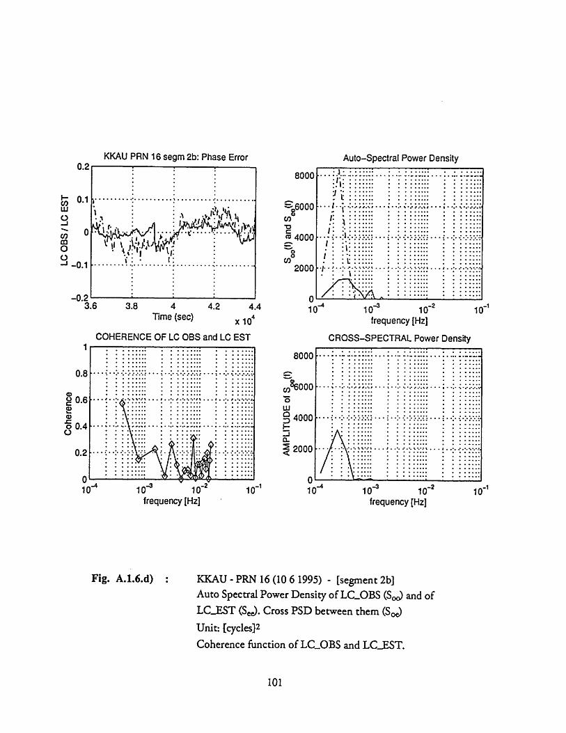
0
0o
00
0
...... .........
..
........ ...... .
........;....... : ........~.................
..
.....
....
........................--s. ···. *
* *.... ..
* *..... .
.....
.......
.... ..
-.. .......
i.......... ...
.............,
...2..s...·
.,,2..
......
.....
... .....~:~~~...=..........,.....
....
.5.·r·····.
.5.'"
-9.--·r
··
··.
··
··
··
()•S
pue (lWO
S
o o
d d
I I
IICI
III0
E -C
')
ow0w
$9,
IS3 0
1/8
80 01
C)
o o
o o
Oo
a o0
(i) S10 30nll~
d•V~
o o
o C
eGO
UJ8t03
I
• I.......
I ..,.... .....
.. ,..,,,
.; ....... ..
.....
.....
...
......
........
........
..........
.......... ...
..
... ...
.. ...
·.8oo~..
o .o.o..
.o,.
o o, oo
o
·.........
..... ..
.........
*. 2*
** .
* *
** *
* *
* *
* *
.5.**
#* *
* **
** *
* e
C
0oo)
0
4)
,0
C,
p4
uU
)vU
)
.- .......... %......
...........
o ,o·,o ,.
,,,,o,o% ,o,
:..0,o
,::::::-:::::::::::::
*:::::. ::: :
............ ......
........ ..
............ •.....
........ ......
o ,....,
,,,, ....,..
.... .......
................
::::::: ..........
:
;* ....
..............................*.............. ..........
* * * *
: : * * * *? * * ** * ****
* * **··~,.....,.........,
'1
----- ---
8
•
I
|
c 3r
I,-
:)I-

KKAU PRN 16 - ASIA 1995 6 10 - Segment 2.c)
0.2
0.1
C,)m 006oS-0.1
-0.2
4
0.2
4.4 4.45 4.5 4.55 4.6 4.65Time (sec)
4.7 4.75 4.8 4.85
x 104
Station: KKAU - Satellite: PRN 16 -Data acquisition date 10 6 1995LC.OBS and LC.EST compared for t=4.40 - 4.85 10 4 secUnit: (cycles}
102
L I I I I I I I I.4 4.45 4.5 4.55 4.6 4.65 4.7 4.75 4.8 4.85
Time (sec) x 104
-I
.\./ I . .. .
..... ... ....... .. ........ . ...... ... ..... ..... . " I... .. i
! !
IL
wCl 00
S-0.1
-0.2
Fig. A.1.7 :
I I I · · r - -

"RESIDUAL" = difference LC Observed - LC Estimated
4.4 4.45 4.5 4.55 4.6 4.65 4.7 4.75 4.8 4.85Time (sec) x 104
o = LC OBSERVED * = LC ESTIMATED
4.4 4.45 4.5 4.55 4.6 4.65 4.7 4.75 4.8 4.85Time (sec) x 104
Fig. A.1.8.a) : KKAU - PRN 16 (10 6 1995) - [segment 2c]
Phase residual LCDIFF, determined as the difference
between LCOBS and LCEST.Unit: [cycles]
103
: segment 2.c)
ý 0

Power Spectra Density: Segment 2c
4.4
-V..
4.4
0.5
4.5 4.6 4.7 4.8 4.9
4.5 4.6 4.7Time [sec]
Fig. A.1.8.b)
4.8 4.9
x 104
10-4 10- 10-2 10
0 10 10-2 10
10 -4 10-2
: KKAU - PRN 16 (10 6 1995) - [segment 2c]PSD of LCOBS, LCEST and LC_.DIFFUnit: [cyclesl 2
104
.. I.. .. .
0.1
0
-0.1
n 93
:i: ::;:::: :1. . . . ,...° . . . . ."I! rS i~i :::i i li iii. ···• ..;f. I\ ...:" .. . " ... ..
:. " : :€,: "\ :•i ::::· · L,#
. .... L ,.; . t • : '
I. ' " ' -. ' ril· · · · · · · · · ·· · · · · · · · · · ·· ·· ·· ·
-1
-1
10-1
| _ · ____ _
" · \·········;Z· 5 : :;;: ; ; i :;; " ":::
: :: .' R :··~· ······-::liii~\ i ·I·~ B·1--·- ···-·---
I --
: ,;;·-
•· • o • • . . . .•· ° ·• • • • . . .
•· ° o • ,• . • o . ..•· • ° • . •° o ° •.. .• ° • . .
•·· ° • ° ,• , . ° . °.
•······ 2·~ . . • ... . . . . . ....• . . . . .
10 -3
KKAU PRN 16: Phase Error
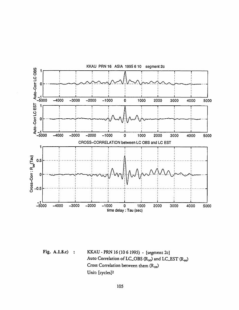
KKAU PRN 16 ASIA 1995 6 10 seament 2c
-5000 -4000 -3000 -2000 -1000
-4000 -3000 -2000 -1000
0 1000 2000 3000 4000 5000
0 1000 2000 3000 4000 5000
CROSS-CORRELATION between LC OBS and LC EST
o.5r.- 00o
2 -0.5
I1
-5000 -4000 -3000 -2000 -1000 0 1000 2000 3000 4000 5000time delay :Tau (sec)
Fig. A.1.8.c) : KKAU - PRN 16 (10 6 1995) - [segment 2c]Auto Correlation of LC.OBS (Roo) and LC_.EST (Ree)Cross Correlation between them (Roe)Unit: [cycles]2
105
cnco
00k 0000o II I I i
1
-0uuuI ___ i I I I I
S................... .....................-
- . . .
I
I
.......
I |
-I I
o • ,Q
I
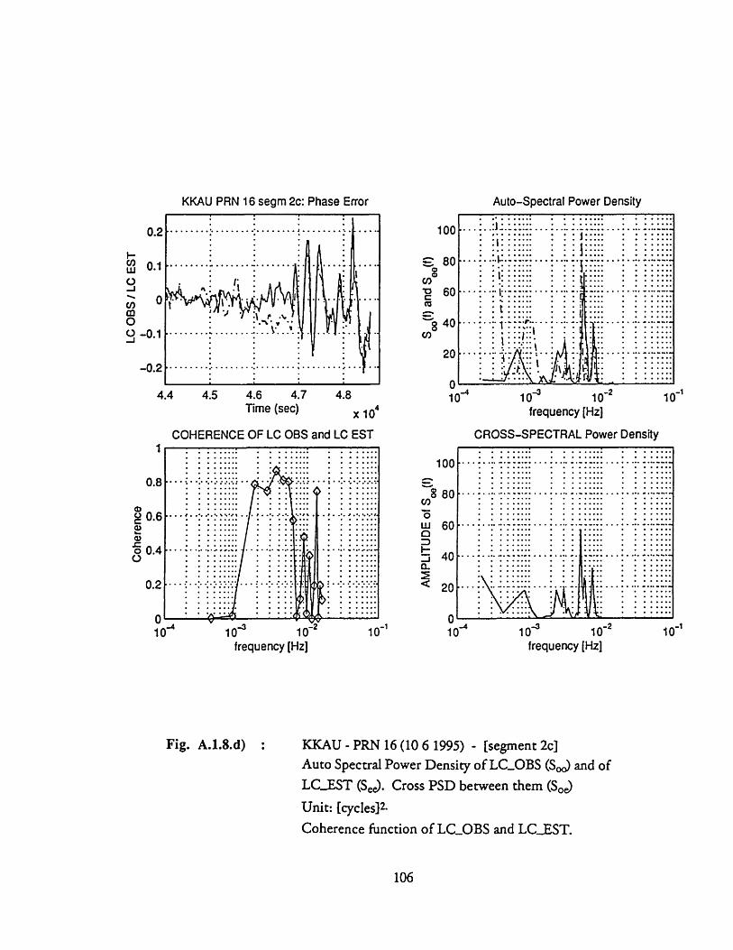
Coh
eren
ce
o .
.b
AMPL
ITUD
E of
Soe
(f)to3
.
0)
00
0o
0 a
0
oC
.J
bi bo
v, cD 0,
SC
LC O
BS /
LC E
STI
Io
oo
o0
-&
Soo(
f) an
d Se
e)o
Oo
O
o
-LC
o0 o o 0 CP
00
I.
° ....
o. ,... .. ......
..
...
o......,
...
..
..... ..
• ...
..........
;.,......
.....
.1.
~~..
......
.... .
.. .....
. ..
...
....
. %
...... :
.......
......
......
......
.:.
......
......
.....
.:
......
......
.. ...
...
....
...
...
....
. ..
.. ...
• ..
....
:...
...
,
o
°
...,
....
..
0o.
....
*..
......
...... *
.... .
......
....
... :...... •...... •..
....
: .....
,,.
*,, ..
,
.•,
o,... .......
.°
...
...
I ...... i
......
i ..
....
.
i ...
....................
...
.......
-r
···~
·~.f
......
..: ..... ..... ... .
..
....."
."
."-.
"
.' "-'."" -
-.•
•
" "''''W'''''"'
'""''
I'
.....
.1
..
....
....
.. ....
......
.. .. ....
,..
*.
=,
,
,...
.••
• I• ,
, |
u,,
,
•.,, ~ ~
~
~
~
~ ·
o,
·.
•..,1•,,,,o,,
1'''''$'''''$'
: :
:::::
::::
:::
::::
:::
'46
-C:)
u
b
*c
re
.. O
d
2w

90 9012 - 60
45.. 30
1 8 .... :-.. .i... ; ...
300270
GPS DATA: receiver location: CENTRAL ASIA
station: KKAU satellite: PRN 20
2 4 6
Fig. A.2.1 :
Time (sec)
400
300
200
100
0
x 10'
acquisition date: 10 6 1995
station: KKAU satellite: PRN 20
Time (sec) x 10'
Satellite visibility chart for PRN 20 (skymap).Elevation and azimuth of PRN 20 with respect tothe station KKAU
107
. ... . -........
............: ...........
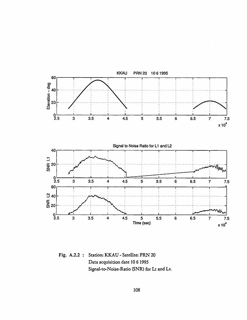
KKAU PRN 20 106 1995
3 3.5 4 4.5 5 5.5 6 6.5 7 7.5x 10
Signal to Noise Ratio for L1 and L2
3 3.5 4 4.5 5 5.5 6 6.5 7 7.5Time (sec) x 10
Station: KKAU - Satellite: PRN 20Data acquisition date 10 6 1995Signal-to-Noise-Ratio (SNR) for LI and L2.
108
' I60
oc
> 2C0)
Ej
- I
I i I I I I i i I I2.5
ci 2zCI,
Cla:zu,
Fig. A.2.2 :
1~ _
i
2.5

GPS "OBSERVED" Phase Residuals for: KKAU PRN 20 - ASIA 1995 6 10
3 3.5 4 4.5 5 5.5 6 6.5 7 7.5
3 3.5 4 4.5 5 5.5 6 6.5--_ _~_ I ^ - -I~rr . I ^ r- ^e I& A W-r r
7 7.5
3 3.5 4 4.5 5 5.5 6 6.5 7 7.5Time (sec) x 104
Fig. A.2.3 : Station: KKAU - Satellite: PRN 20Data acquisition date 10 6 1995The observed phase residual (LCOBS) is compared with themultipath phase error estimated from the SNR (LC.EST).Unit: [cycles]
109
I --1 -- I--- I I I
I I
I· . .... I
· · · · ·
...............
I i i i
•o•r.-
-- v=.•

KKAU PRN 20 - ASIA 10 6 1995: Reduced set of data
6.6 6.7 6.8 6.9 7 7.1 7.2 7.3 7.4 7.5Time (sec) x 104
I -I r
A1...... i! ... ..!.. ... 1. .~... ; .-
'1 1 i'; i'iIl
;I' I I : I : II
. ........-
.•! ·- -- -.. . t- · · ·.. . . i ;. .. . ..J .I "
6.6 6.7 6.8 6.9 7 7.1 72 7.3 7.4 7.5
Fig. A.2.4 :
Time (sec) x 104
Station: KKAU - Satellite: PRN 20Data acquisition date 10 6 1995LCOBS and LC_EST compared for t=6.5 - 7.5 10 4 sec
Unit: (cycles]
110
I I I I I0.2
0.1
1
-0.2
0,3
6.5
0.15
0.1
0.05
-0.05
-0.1
-0.15
n0 6.56.5
*I j · ·
I I
-
-
-
SI I
..........
-
-
-

KKAU PRN 20 - ASIA 10 6 1995 : Segment 2.a_
6.55 6.6 6.65 6.7 6.75 6.8 6.85 6.9 6.95Time (sec)
7
x 10
6.55 6.6 6.65 6.7 6.75 6.8 6.85 6.9 6.95 7Time (sec) x 10
Station: KKAU- Satellite: PRN 20 - [segment 2a]Data acquisition date 10 6 1995LCOBS and LC_..EST compared for t=6.5 - 7.0 10 4 secUnit: [cycles]
111
0.2
0.1
0
-0.1
02
6.5
0.2
-0.1
-n 96.5
Fig. A.2.5 :
1 1 1 I
F -

"RESIDUAL" = difference LC Observed - LC Estimated
6.55 6.6 6.65 6.7 6.75 6.8 6.85 6.9 6.95 7Time (sec) x 10
o = LC OBSERVED * = LC ESTIMATED
6.5 6.55 6.6 6.65 6.7 6.75 6.8 6.85 6.9 6.95 7Time (sec) x 104
Fig. A.2.6.a) KKAU - PRN 20 (10 6 1995) - [segment 2a]
Phase residual LCDIFF, determined as the difference
between LC..OBS and LCEST.
Unit: (cycles]
112
U.1
0.05
u. 0
-0.05
-0.1
nf 1
6.5
: segment 2.a,,

*•**
...
***
* .
•...
* ***.
...
..
•... t...r .......
.....
.... .
•, ....
.... ..• ..
...:...:....
*...
.. ..."
.*. ,.*. .. ....
• ... ...
....:::::::::
::::
I
S8
0
"1J OOSd
....•.
.......... c6
jNuC
o
.N.
.... .
........... C
%-6
····........
• .
.
.... ; ~ c,.,.... C
..... •U,
t e -
O
=
c'M
I I
* * .*
* .* *
• * * *
.* * * * * *
* •
... .*
**.
**
**
**
**
**
**
...)...*...**...* ...
.......................
..
.. .
..
..*... .....
*...•....
• ..
l. .. ·
', .
..*
* _
• .S •
."
**
...
:...:..*...
• .: ...
... : .... :. •
•. ·
··
·'·
·~ .
•'· '.·· ·
··
..
i l
I i..'~
~~
~
IS3 01 o O
Sd
*********************
.. .
....... ..
., ..
..... .
..
..
...
... ...-.
. ...... ...
...o
........: .-•.-
.:::.:.:.::::.:::.:..
1...:..1
.:
....
: ...
• • .. ,.
...••%
••
..
• •..
°.. ·
i a
I *.....~
oC)
o c
JJ1 07 l0 G
Sd
1=la 1 01
11
IS3 0
"
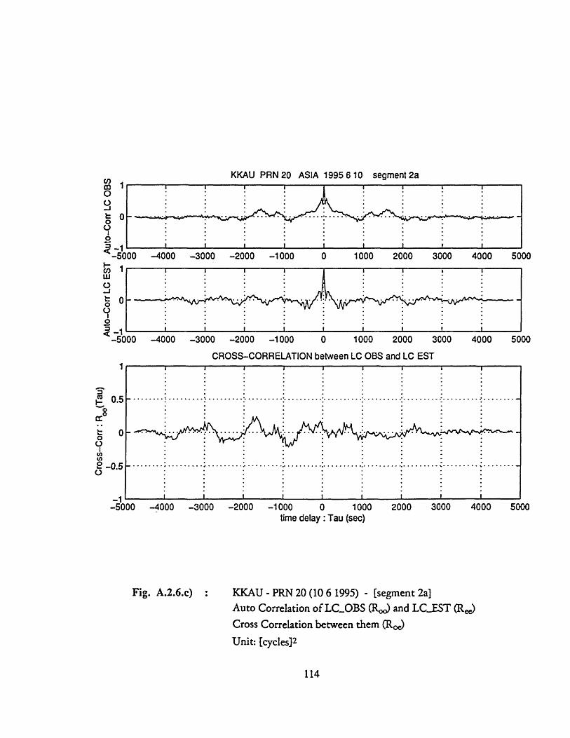
KKAU PRN 20 ASIA 1995 6 10 seament 2a
-5000 -4000 -3000 -2000 -1000
_I
-:UUU -4UUU -jUUV -iUUU -1UUU
0 1000 2000 3000 4000 5000
0 1000 2000 3000 4000 5000
CROSS-CORRELATION between LC OBS and LC EST
-5000 -4000 -3000 -2000 -1000 0 100time delay : Tau (sec)
Fig. A.2.6.c)
0 2000 3000 4000 5000
KKAU - PRN 20 (10 6 1995) - [segment 2a]Auto Correlation of LC.OBS (Roo) and LC_.EST (Ree)Cross Correlation between them (Roe)Unit: [cycles] 2
114
cl)
0
0 00
0I I I I I I I I I
I I I I I I I ! I
02t,,o
InU)
0C')
0.5
-0.5
I . I
I I
I i i "
| I • m I
I I I I I tI I I I-Ir~AA IAAA ~AAA ~AAA
.. ... . .. . o•.
. .. . .. ... ... ... .. ... .. ...
........... 2···.. .. ·
I I

c
0
-t-
0
V.-
(i) "s pue (
OO
..... ..
..
.o...... ...
... ... .......
.'. ......
°...;........ .
..
.
..
..
.
..°°°....
...° ...........
.°
.
: 7... ..
..
......
...
...........o. ...
•%.•
.•. .
~ ·
·° %.• .. •. ••°°
.%°, ..° ...........°...°
.;
°
IS3 71 S80o 31
C)
0 U
)
(I) S 0o :ifi.LIdV
4W
0co
co
OO
uOJLoo
S
.°.....
°.....o
........
,
o...
o.
.o
•· .
° •··
.....
°..... ...
°°°°.... °°
......... ....... ........
..... ..
.........
....
!i ! ! ! !. ...
....
°o. .°°
,o.°°o
°°.~o°
7°° ........
.° ..
...o ..
...
.. .
...
o...............°
.... .
°... .
.°...............
..............
.°° ~
o
...
.•..
..
|...... °......
.................. ..........
::::::i:::::~:::::::::::: ::::::::.
.°
..°
°°o
,o. ,°°
,•.
.o....... ..
°,
,
...... ...... %
...... ............
.. ..
...... ...
... .
...... ......
...
... ..
.. .
.. ..
.. ..
... ..
I>0'oT-
>
0r0)=
O0
i m
i
g
<<
•
N
| •
orc
-
c=) V

KKAU PRN 20 - ASIA 10 6 1995 :Segment 2.b
7.05 7.1 7.15 7.2 7.25 7.3 7.35 7.4 7.45Time (sec)
7.5x 10⁴
7.05 7.1 7.15 7.2 7.25Time (sec)
7.3 7.35 7.4 7.45
Fig. A.2.7 : Station: KKAU - Satellite: PRN 20Data acquisition date 10 6 1995LCOBS and LCEST compared for t=7.0 - 7.5 10 4 sec
Unit: [cycles]
116
U.2
0.1
w
0
0 -0.1
-0.2-0.2
7
0.15
0.1
0.05
0
-0.05
-0.1
-0.15
-0.2 7
.I I .. . I...
. . .. ......... ... ..... ...... .. .... .. . ......... . .. .
... ........... ....
-V ....... ... .."................... .......... ......... . . .. ! . .. . . . . . .. . . ... .- :. ...... ..
7.5
x 104
X A
-
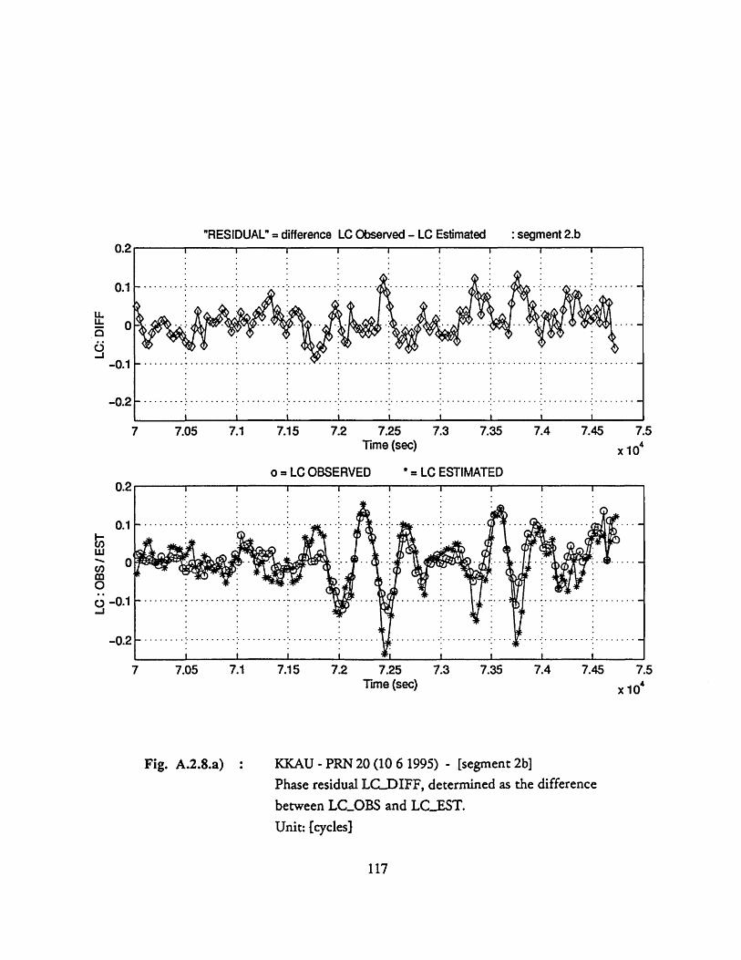
"RESIDUAL" = difference LC Observed - LC Estimated
7 7.05 7.1 7.15 7.2 7.25 7.3 7.35 7.4 7.45Time (sec)
7.5
x 104
o = LC OBSERVED * = LC ESTIMATED
7 7.05 7.1 7.15 7.2 7.25 7.3 7.35 7.4 7.45 7.5Time (sec) x 10,
Fig. A.2.8.a) KKAU - PRN 20 (10 6 1995) - [segment 2b]Phase residual LC.DIFF, determined as the differencebetween LCOBS and LCEST.Unit: [cycles]
117
0.1
-0.1
-0.2
: segment 2.bA A
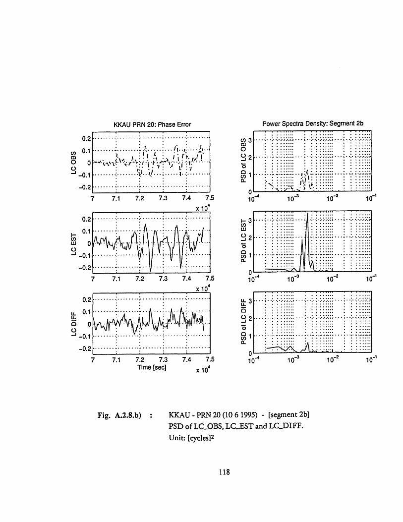
LC D
IFF
ila3 C
D
CD
0 Z
4
i-t
Oo o
00C
-4 -4 -4
PSD
of L
C DI
FFC
0 -&
r)
w
'Ia 0
..... •.
....
.•..
....
.
.I...
......
....
.....
•...
.. •... .. .
... :
..... ..... ..
.....
....
I ..
.. ·
.
°°,.,•°,,..•.°.
.•I,
...
.... •..
....
,...
::::::
::::::
:...::
::::
LC E
STI
I
io
-0-
' t)
....
.1.
.....
.... ........
~3.. .
. .
PSD
of L
C ES
TO
r"
~C
A)
-4 -4 -4 ila -4 -4O
sh
,
LC O
BSI
I00
00
-I,
..1
: "
;
:--" '7 "--'·
.. .
....
..
r --
.:
PSD
of L
C O
BSC
.
! )
N
CJ
........
....
......
......
...
..,°
.I,
.,,
.. °.......
0 ::::::::::
C) .......
.. .
.. ........
-.--
.°
a-.
"I
·2•·
·
···
··
2:|
.°
•·t·
· ·
·•
• •·
·5···5
....
....
. •.~
..~..
.°,°,,•..,,.•.,,,.°•,
.o,,,•,.,,,•.,.,,,.,.
0 alaý4
C
CL
L...
....
......
..........
....
....
..
..,.......•.........
• .• .•
.. ..
... .
...
:..
S.....
.....
..........
,.,..•.,.···
·...°
•,,,,,i o,,o%, ,,,,.,
··,,·.·,.,..·.·,·5
··,
r°.
°e
°°.
#,
.°° •°
.. ..
·..
..
.. ..
)···:
··ii··
···i
?:i
..... I ....
I ...... i
II:
i:::
::::
::i:
::::
:;:::
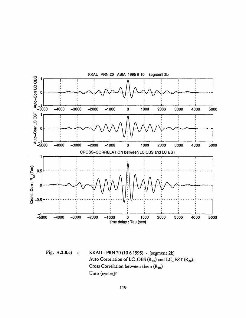
KKAU PRN 20 ASIA 1995 6 10 seament 2b
0 1000 2000 3000 4000 5000
-- I,LeaAA h AA A•l•l i AA A
I I I I
I I I I
-30UU -4UUU -SUUU -zUUu -1 UU
I I I I
l lI _ I -_
0 1000 2000 3000 4000 5000
CROSS-CORRELATION between LC OBS and LC EST
-0.5
_t
-5000 -4000 -3000 -2000 -1000
Fig. A.2.8.c)
0 1000 2000 3000 4000 5000time delay : Tau (sec)
KKAU - PRN 20 (10 6 1995) - [segment 2b]Auto Correlation of LC..OBS (Ro,) and LC_EST (Ree).Cross Correlation between them (Roe)
Unit: [cycles] 2
119
O
o-J II-0
-500C -4000 -3000 -2000 -1000
SI I I I I I I I
.- .. o... . o ..... . . . . . .. .......... ........
.. .. . . . . . . . . . . . . . . . . .. . . .. . . .. . . .. .. .. . .. . .. .• o,
•··~~ °·· · · · · · ·· o~. ° .~~~~~~~· ( · · · · · · '' ~ ' ·
I I I I
- -
• . . . .I
i i I I
_I ·, ·
r I I I I
i if

Coh
eren
ce
o
o9.
b)
bo
LC O
BS
/ LC
EST
I I
0 0
hr)
-L
AM
PLIT
UD
E of
S
(f)
-L
r O
-9
O
C
C
0oo
0
0
C-L
C0O
L
L
o
o0
..A
i
S (f
) and
S
(f)
No
oC>
C
) C
C)
C)
C
.LC
'o
0 :r (b 0C
) 0 0 ci. 0,
o o
o0o
C 0L cA
........... i..
......
......
.
.X......
......
......
. ...
......
.....
............
....
..·.
..'..'
·. ....
'r'............
1::::
::::::
:: :
: :
: :
: ::
: :
:
...;..~.;...............~~
:::
::::
:: ::::::::::.:
.::::::
::::
.....
......
......
. .........
~~~......:..
....
*
......
~...
: ..
.·......
... ............
"..
....
:.
.....
....
....
....
.. ......
: : :::
::::
::::
:::
::::::~::::::::
....
.........................
......
......
......
. ....
.. ..
°...........°.
.......°
..,.......
......
.
....
....
..
......
....
~~....
......
..
-.--
,--
**- -
- -
--
-•. -
S.
.
.. .
*....
..
..
.. ....
.....
.
..
..
."
..
.. .
.•
.A
:)
)
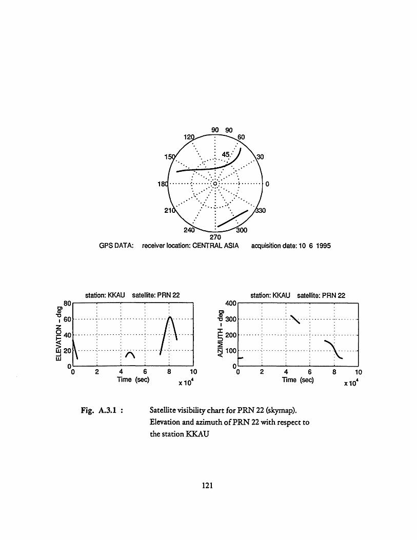
909060
45*-330.............
18 . ..... .. .-... : " .
21
240 300270
receiver location: CENTRAL ASIA acquisition date: 10 6 1995
station: KKAU satellite: PRN 22 station: KKAU satellite: PRN 2240C
o 30C
20C
10Cr
2 4 6 8 10Time (sec) x 104
0 2 4 6 8 10Time (sec) x 104
Satellite visibility chart for PRN 22 (skymap).Elevation and azimuth of PRN 22 with respect tothe station KKAU
121
1
GPS DATA:
Fig. A.3.1 :
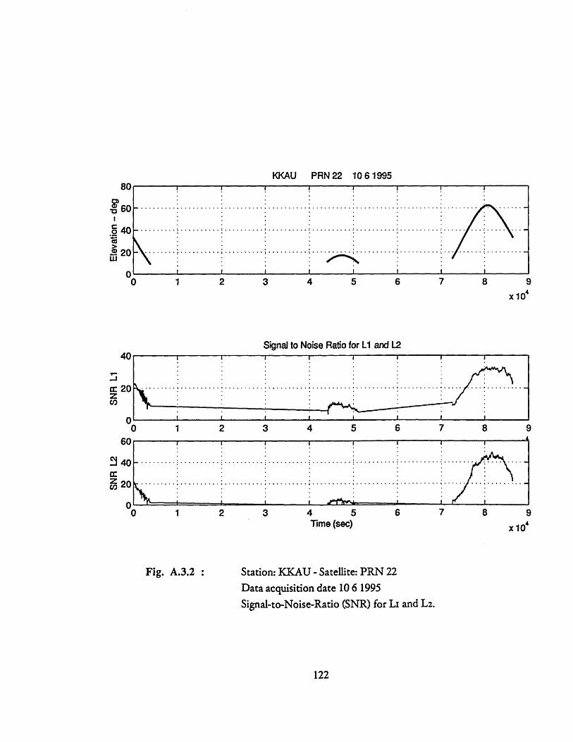
KKAU PRN 22 10 6 1995....... I
0 1 2 3 4 5 6 7 8 9x 10
Signal to Noise Ratio for L1 and L2
0 1 2 3 4 5 6 7 8
4 5Time (sec)
Fig. A.3.2 :
9
x 10'
Station: KKAU - Satellite: PRN 22Data acquisition date 10 6 1995Signal-to-Noise-Ratio (SNR) for LI and L2.
122
K
80
. 60
.o40
S20
0
40
0
60
40
20
0
S......................................I...................I............
. . . . .. . . I
. .... .... . ... . ... .. .. . .. . .... . ---
0
SIi I I
- I -A - - .. .L - - - - i , - -,
,
..........-
I ! I r
.... ....... ..... ... ........
. . . I..
..
I !
|

GPS "OBSERVED" Phase Residuals for: KKAU PRN 22 - ASIA 1995 6 10
.. I r% rf C %XAnr%\• I ^ I•%•IIl& A 11ll
1 2 3 4 5 6 7 8Time (sec)
9
x 10'
Station: KKAU - Satellite: PRN 22Data acquisition date 10 6 1995The observed phase residual (LCOBS) is compared with themultipath phase error estimated from the SNR (LC..EST).Unit: [cycles]
123
ft ^
C 0.1
Ca,0OU -0.1
-0.2-0.2 0
Fig. A.3.3 :

KKAU PRN 22 - ASIA 1995 6 10 :segment #1
500 1000 1500 2000 2500 3000 3500Time (sec)
1000 1500 2000Time (sec)
2500 3000 3500
Station: KKAU - Satellite: PRN 22
Data acquisition date 10 6 1995
LC_OBS and LCEST compared for t=0.0 - 3.5 10 3 sec
Unit: [cycles)
124
-0.1
-0.2
-0.1
-0.2
I B I
1* .1.
\. * • -... , .-" ' f '~ * / I .- " -. ' . : ". •- . \ S - !-
* I~i li * / ' '.......... ........... .................. ...... .... .. -..... .. : ........ .: ....
I iI· \IP500
Fig. A.3.4 :
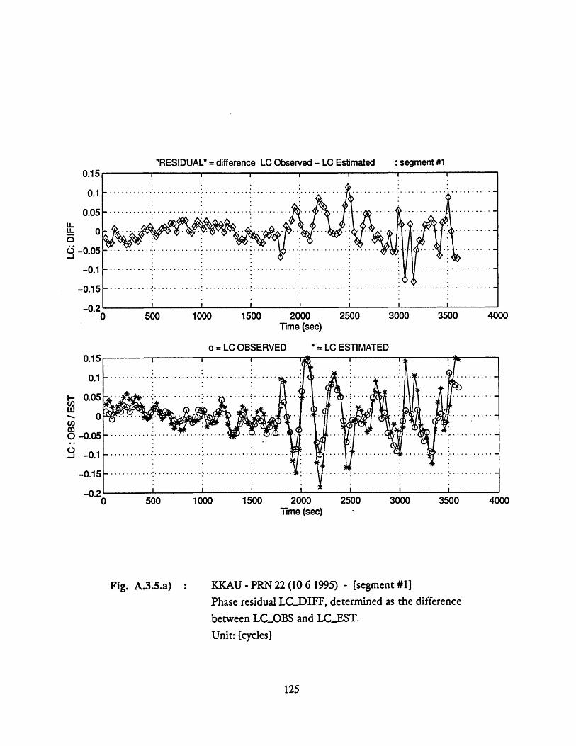
"RESIDUAL" = difference LC Observed - LC Estimated
1000 1500
o = LC OBSERVE
2000 2500Time (sec)
D * = LC ESTIMATED
3000 3500 4000
500 1000 1500 2000 2500 3000 3500Time (sec)
4000
Fig. A.3.5.a) : KKAU - PRN 22 (10 6 1995) - [segment #1]
Phase residual LCLDIFF, determined as the difference
between LCOBS and LCEST.
Unit: [cycles]
125
0.15
0.1
0.05
0
-0.05
-0.1
-0.15
-0.2C
- - - - - - - - I . . . . .
....................... ........................ _
500
0.15
0.1
0.05
0
-0.05
-0.1
-0.15
-n 90
: segment #1
-
...... .......-..... ....
........................ . . . .
... ,
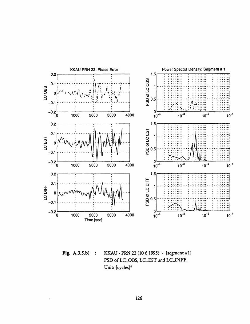
Power Spectra Density: Segment # 1
. . . .,. , . * * * . ...... * * * *****
. . .•..... . . ....... . . . .•....
.. ., .. ... ., . o . . ........ . .- -.. . . . .. ... .....• • • • •.. • • .. . • • • • . ••• i-i-~.iii • •. .. •.• . • · ·· · ·~S~" ,.,. • .,i.• • •
........... .......... i-..
............. .....
.. ......... .....
......... ..........
1000 2000 3000 4000
1000 2000 3000 4000
1000 2000 3000 4000Time [sec]
Fig. A.3.5.b) KKAU - PRN 22 (10 6 1995) - [segment #1]
PSD of LC.OBS, LCEST and LC..DIFF.
Unit: [cycles] 2
126
0.2
0.1
0
-0.1
_n
0.2
0.1
0
-0.1
02' 9
- 0 10 102 10-
.0
0.5
0
0.2'
-0.1
A',
10-2 10
- .0
0
10-2 -110
KKAU PRN 22: Phase Error
2
'"'
10-
• , , , •.. . , . . . .. , . .• o • .• o• . . .. •• • • . o . o o o , .• • o • • ,o .• • • o"oo, • • • o •• • • ., .
•" .• o" " ,o , • • . . o • •,•' o • .•o.. • . . . •, • • .o ,
•·· · · · ~~· ·• . ,,.,.• , . ....... , • • ••..
•· • .• o, . • .. .. . • . .•· • • ." " .. . , . . .. .. , • ..
•·· .• •" " .. , • • .. ... • • . .•· ·• · ·.o..• ·. . .. . • • •...•· . • •" " ,, . . . .. . • , • .
•·· .. ," " .. , • . . .o . , • ,.i e ....... ···r--rr··· ··rrr• • • ,,
10 -
rrr····················
~·L· ·· ·· ·· ·
· ·I
- --o - , , . ....
: : ::::::.:. . .. ...• ·., .o,., • .. . .• o. , • . . . .
-
.. .. .. .
--,o,
1010I
r
i
10
1040104
.. ..
................................ . .....
)

KKAU PRN 22 ASIA 1995 6 10
4000
40(2000 -3000 -2000 -1000 0 1000 2000 3000
CROSS-CORRELATION between LC OBS and LC EST
-3000 -2000 -1000
Fig. A.3.5.c)
time delay : Tau1000
(sec)2000 3000 404
00
00
KKAU - PRN 22 (10 6 1995) - [segment #1]Auto Correlation of LCOBS (Roo) and LC_EST (Ree).Cross Correlation between them (Roe)
Unit: [cycles] 2
127
m i0O
o-- Io
o1
-4000 -3000 -2000 -1000 0 1000 2000 3000
1
-0.5
1
I I I I I I I
I I
-4000
segment #1MJ
-- 6

Coh
eren
ceo
o bo
AM
PLIT
UD
E of
Soe
(f)m
.
QD
O
0 C
0 0
C)
0 0
"C
h0
k
LC O
BS /
LC
EST
-0D
Soo(
f) an
d Se
e(f)
0 0
0 0
0 0
-L '1
0 C,
0 o 0 td'
V0 c/-
o t-' n.......
...............
.- .. ... .,, ........
..... ..;
..... ... ..
.......
,....
•
.....
•.•1,•
••
..
:
.:
..
.....
. ...
...
.....
. ....
.
...........t...• .......
..........
....
......
...
..
X.·
·:
··
1
··
:···i
··
:·
·
__
.•
.".
..
.•...... .............
°°.o °...
o°•.
o~o•
.......• .
•.. o
..
..
... .
..
.. ..
....
..
....
....
. .
......
: ... .. ...... I
:) :}L
)-o
......
;.....
..
...
..
..
..
.
....
·.....
..
......
...I..
......
...-....... ...........
1.......
..
.....
.......
• .
•':
:
:
:··
....·...,.,..i,.,.,.....i.....,,.•,.
: : : ! !:
." ........ :
• ,I
~=
°·
I····
........
..
....
. ...
...
. ....
.. ...
...
....
...
..
.....
....
. ..
... .. ..
..... .
.... ...
..
..
..
.... .............,.....
"'
'' .....
·..
.·
··
·..
.''
'

KKAU PRN 22 - ASIA 1995 6 10 :segment #2
4.4 4.5 4.6 4.7 4.8 4.9 5
4.5
Fig. A.3.6 :
4.6
Time (sec)
4.7Time (sec)
x 104
4.8
x 104
Station: KKAU - Satellite: PRN 22Data acquisition date 10 6 1995LC.OBS and LCEST compared for t=4.3 - 5.1 10 4 secUnit: [cycles)
129
I I - I I I I I
I .'.
.. . . ........................ . ..I ... . •
I" ' " "I |•J . '.2J \" ~
1 - *..* :A .
I .1 .°I- .° ° ° ,.. .:I1 ...... :•i ....... :..................
I . I ••I- - - (
-0.
-0.4.4
- .. ... ... ... ... ... ... ....... .. :. . . ... . i. ' .A- i .. .. . ......... . ,. ........ . ... .. ............... .
r
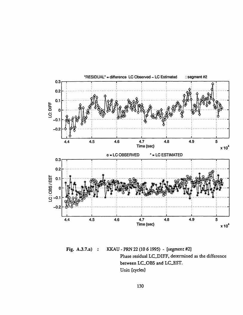
"RESIDUAL" = difference LC Observed - LC Estimated
4.4 4.5 4.6 4.7 4.8 4.9 5Time (sec)
o = LC OBSERVED * = LC ESTIMATED
x 104
Ii i1 II
4.7Time (sec)
4.9
Fig. A.3.7.a) KKAU - PRN 22 (10 6 1995) - [segment #2]Phase residual LC..DIFF, determined as the differencebetween LC..OBS and LC.EST.Unit: [cycles]
130
0.3
0.2
-0.1
-0.2
I i
4.5 4.6
x 10'
: segment #2
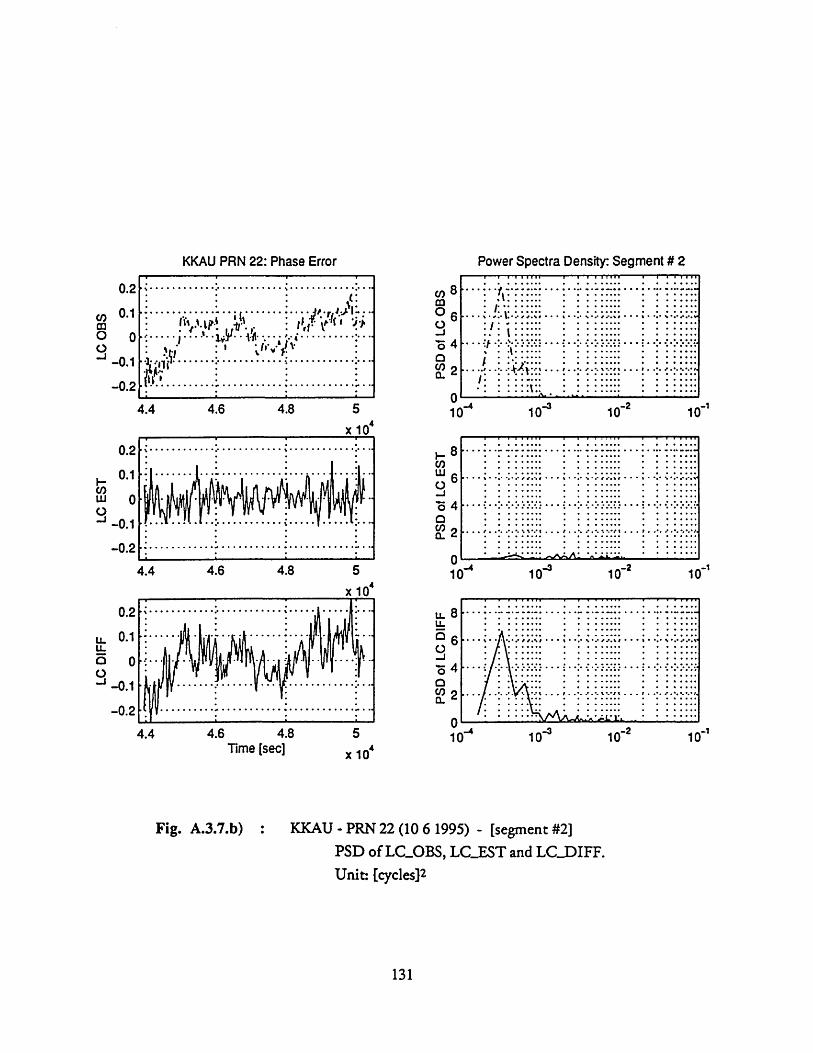
.....
......
..
" . ...
...
....
".
...
.S ....
..... .....
•··i· ·
·'
.•
-.•
CO
(1
O
oS O
O
$80 "1G
do OS¶l
..
..
.. .
.....
*1
C
M
.'.... t .d• • •...
....
t
C;
C;
c;
o.
o
oo
•
0
•
04
··, ·
· I··~
··I
I~
$80:3"i C
..°.....°.............
...
°. .
...
.°. °. .
.° ...•
...... ..
.. .. ..... .
....
I C.
.., ..
.' ..
.,
....' .
• .. .
.... .
..... .
...
, ..
., .,: .. .
.. .* .
.. .,. .
..
.......
•!.... .
......
.... ......
ILS3 0"10 (o Sd
9o0U
cq 1-C
Cq%
,
o
T
e
"oto
Sr
Ov* 0
oo
3
3
N
--O
6o
C
.-IO
01
0 G
O lSd
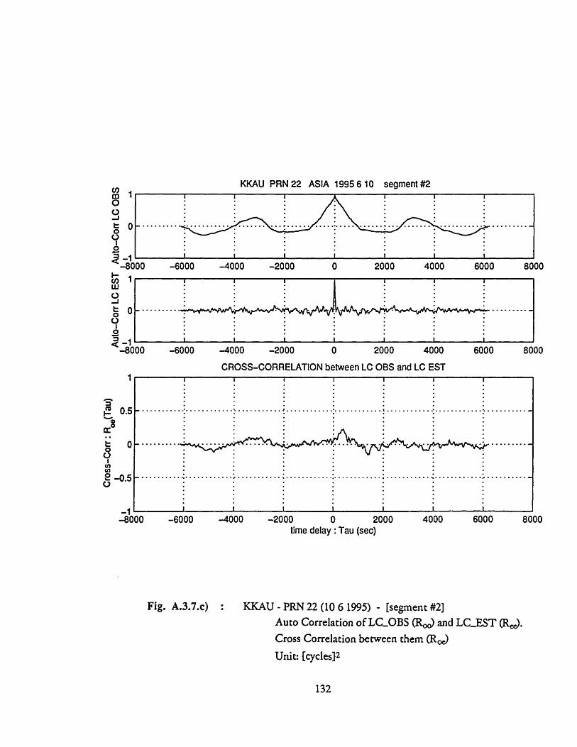
KKAU PRN 22 ASIA 1995 6 10 segment #2
-6000 -4000 -2000 2000 4000
8000
6000 8000
CROSS-CORRELATION between LC OBS and LC EST
.... ...... ........... .... . .......
-6000 -4000 -2000
Fig. A.3.7.c)
time delay : Tau (sec)2000 4000 6000 8000
KKAU - PRN 22 (10 6 1995) - [segment #2]Auto Correlation of LC_..OBS (Roo) and LC_EST (R,).Cross Correlation between them (R0e)Unit: [cycles] 2
132
ml00-.Jt 0o
0--80-80(
uJ
O
0oI?0..
4q. - a
I I I I I I I-60 -40 -20000 400 600
-8000
2u(I,O(I0oC-)
0.5
0
-0.5
00
--
c-6000 -4000 -2000 2000 4000 6000
O W • ° °
"'' ., ,·- ·,·
-1 -
-8000

o 0
o 0
0 0
(1) "s pue (1)00°
..... .° ....
.............
......*" ..
.. ...
."
.:
..:. ......
:" ." ": : :
.. ...O ..
.. ..
o.. .• .
....
... ....
° .
...
°
... .
....
%.
...
°.
..
...
..:
°... °.......*... .
. .... ...............
.................. :
.......
. ....
........
.. ... ....
.....
... ..
.,.%
........... .
.. .,
.......... :.
...
.......
.....
...
....
.. ....
• °
°
• °
°..
T-
0 Q
-N
I I
1s:: o"Is
80
31
"
o o
o
0o
U
o) 0
1C)
(I)C°S Jo 3GflllY
dVW
OD U
o
o d
e0ue~ey00
>,
U)
iri
O0(L-.3
(1)0Q
.oC,0
ICcuoC
...........
..............
......
...
..........;
* ..·****.......* .....
*
......
... .... .
.....
......°......
.. .
...... ...............
............. .....
....
°... ° °... °
...
° .. .
.. ...
°.°.°.
..
I17-
C
t4.40OC/)ao14
t 6-)
0I.)04-
.......:......o
.......
..
..
:: : :::·::::::~::''::::::::::::::::
..................... ?...... ......
,°**oooe***o.*eoo..eoo·o
·oo.,.,···
... .....
... ..
.....
.. .
....... ....
...
... .. ...... .. .......
......
:::::·::::::: :::::: ::::::::::::...........
...............
...
..
..... .
...
....... .
.....
.... ~
. ....
.• .
..
...
...
" . .: : .
...
:::::::::::::::'::::::!::: :~
....... :...... % ......
....... :......
............. .
.. ..........
......
•· ,··~
· ··
··
·•
,
Io-C
.. ... ..-
..
.... ...
...
Cl
............. ......
..··-
cv:
,
:) T-

KKAU PRN 22 - ASIA 1995 6 10 : segment #3
.2 7.4 7.6 7.8 8 8.2 8.4 8.6Time (sec) x 10
• , " -- , - -.. ....... .... ...... ..... ..... . ... ..'".:. . -..
VrI- I
.,.. .-.--". =.'... . .... . . .. . . .. ..... .. . " . .... \... .. .... ... ,
Time (sec)8.2 8.4
Station: KKAU -Satellite: PRN 22Data acquisition date 10 6 1995LC_OBS and LC__EST compared for t=7.2 - 8.7 10 4 secUnit: [cycles]
134
0.2
0.1
-0.1
-0.27.
....
! I ! I
0.1
-0.1
-n o7.
.. . .
Fig. A.3.8 :
x 10
S . ... . .... ..
1-
I
............. ........... ...........
I/
2-

"RESIDUAL" = difference LC Observed - LC Estimated
7.2 7.3 7.4 7.5 7.6 7.7Time (sec)
o = LC OBSERVED * - LC ESTIMATED
7.3 7.4 7.5 7.6 7.7Time (sec)
7.8
x 10'
Fig. A.3.9.a) : KKAU - PRN 22 (10 6 1995) - [segment #3.a]Phase residual LC_.DIFF, determined as the differencebetween LC.OBS and LCJEST.Unit: [cycles]
135
7.8x 10⁴
0.05
0
-0.05
'-1
: segment #3.a)
7.27.2

"RESIDUAL" - difference LC Observed - LC Estimated
7.8 7.85 7.9 7.95 8 8.05 8.1 8.15Time (sec)
7.8 7.85 7.9 7.95 8 8.05 8.1 8.15Time (sec)
Fig. A.3.10.a) : KKAU - PRN 22 (10 6 1995) - [segment #3.b]Phase residual LCDIFF, determined as the difference
between LCOBS and LC.EST.
Unit: [cycles]
136
8.2x 10'
8.2x 10⁴
: segment #3.b)

"RESIDUAL" = difference LC Observed - LC Estimated
Time (sec) x 10
8.2 8.25 8.3 8.35 8.4 8.45 8.5 8.55 8.6 8.ETime (sec) x 10'
Fig. A.3.11.a) KKAU - PRN 22 (10 6 1995) - [segment #3.c]Phase residual LC-DIFF, determined as the differencebetween LCOBS and LC.EST.Unit: [cycles]
137
: segment #3.c)
5
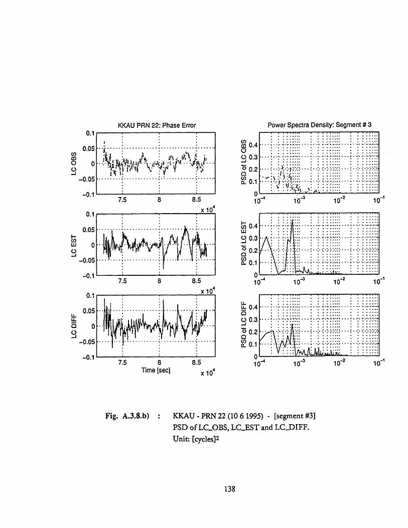
LC D
IFF
IS0
b
-&
l-
m
o1
0 "
--
PSD
ofc•
o...,
i•
a
o
LC D
IFF
o0
LC E
ST00
c o
o0
-m
o
mr
..
PSD
of L
C ES
T
aj
i4 't
....
....
.. ....
0 ...
......
....
... .
....
.. ....
*:..
.... ..
..............
"'"
•"
"
LC O
BSI
0 0
Po
o
0, L1
a:-~
-~L
-c·
~-
r~'
-L·
-Z-r
e
-CC
r~T
L
·,. :JE
.'h
··
4c·
YL
~c' r
rC1~
~
,F·
r.·;
PSD
of L
C O
BS
a Co
CoC
C>
CI .
..
.
.• ..
0
.......
"•""
:-'L
"":~
~~
""
"",,
• .. ...... .... •.. ...
....
... ..
•..
..
•
..
...
..
.. .
..
...
..
...
o
.::. ::::.:.
::. ::::.::
..
...: ...
·I...·
·· •.
..· ·
-4 iýn
-D 3 <c C1)
0c~
O
ct R.
·
z....
.~c~
r.
.0
" '
....
i.....
. ''
''... ..
..
I::::
::::·:
:::;::
:; :
: :
:
-AC
I I
1 -~
I
!!!

KKAU PRN 22 ASIA 1995 6 10 segment #3cn
-1 -0.5 0 0.5 1
CROSS-CORRELATION between LC OBS and LC EST
-0.5 0time delay :Tau (sec)
0.5
1.5
x 10'
1.5x 10
Fig. A.3.8.c) : KKAU - PRN 22 (10 6 1995) - [segment #3]Auto Correlation of LC_OBS (Roo) and LCEST (Re).Cross Correlation between them (Ro)Unit: [cycles] 2
139
0
o-1
0Q-1.5<;-1.5
c-)
-J
0
o,1
-1 -0.5 0 0.5 1
-1.5
1
0.5
2 -0.50.
I II I
I I I I I_4
-1. 5_ _.· ·
Q -'
L°°°
° ..... ..... ...--
L

00.
o O3
a.C
'
CCItw
o-o
oci
C;
o o
o) o
to C
0 C6
.........
....
..
°...
... °.. .
...... ...
....... .....
......
::::::::::::: ::::::::::::::: ::
.............
.................
.
.........
...............
........ .....
% .. .
.. ..
...
....
......
--CO
)E
iLr-
IS3 1 1 S
O
8001
o o
0
0o
to
C)
L)
c'J 30~ nr~-
o o
'eg
eO
lO
i-.
..
.. ..
.....
...
...
...
.... .
: :. :. :::
........ ...
......... ..
.....
.. .. .....
..... ..
....... .
......
...... ....
... ....
... ....
... .
... .. .
..
............. ......
;...............
.....
... .. ..
...... .
... .
.. ....
... .
..... ..
.... .. ...0 .. ...
.... ...... .. .
..
•.. .
°..
... .... .° .%. ...
°. .
0.
o..
...
.................. .... ..
..
.I
...
....
...
...
...
C
o%4-4
00o144)o0'a;
1 ·
·
..
•
|
(1) S pue (0)00SJ
(11
3-
.. i
.....r········
rr········
..
*.
·..
:...... ..............
:... ,.
...........
..
.... :...... ......
.............
c........
··~~~~'.............•~r·~· ,
..o...
....... .....
€ TOr-

90 90
21 0240 _ .300
270GPS DATA: receiver location: CENTRAL ASIA acquisition date: 10 6 1995
station: MANA satellite: PRN 2640C
300
200
100
1 2 3 4 5 6Time (sec)
Fig. A.4.1 :
x 10'
station: MANA satellite: PRN 26
1 2 3 4 5 6Time (sec) x 104
Satellite visibility chart for PRN 26 (skymap).Elevation and azimuth of PRN 26 with respect tothe station MANA
141
L : _ I
.. .... ..... ... ........... .
)
I = l i |
E
.. ............: .....* ......'

MANA PRN 26 10 6 1995
1.5 2 2.5 3 3.5 4 4.5 5 5.5 6
x 10,
Signal to Noise Ratio for L1 and L2
1.5 2 2.5 3 3.5 4 4.5 5 5.5
1 1.5 2 2.5 3 3.5Time (sec)
4 4.5 5 5.5 6x 10'
Station: MANA - Satellite: PRN 26Data acquisition date 10 6 1995Signal-to-Noise-Ratio (SNR) for Li and Lz.
142
I I I I I
60
i 400
> 20
0
1000
500
n
1
60
40
20
n
SI I ! L I I
I I I . I I I I I
I - I I i
Fig. A.4.2 :
i
tV
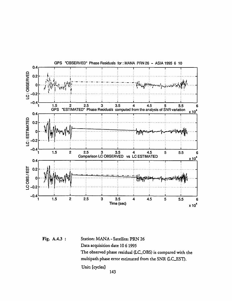
GPS "OBSERVED" Phase Residuals for: MANA PRN 26 - ASIA 1995 6 10I I I I I I I i
1 1.5 2 2.5 3 3.5 4 4.5 5 5.5 6GPS "ESTIMATED" Phase Residuals computed from the analysis of SNR variation x 10"
1.5 2 2.5 3 3.5 4 4.5Comparison LC OBSERVED vs LC ESTIMATED
5 5.5 6x 10'
1 1.5 2 2.5 3 3.5 4 4.5 5 5.5 6Time (sec) x 10'
Station: MANA - Satellite: PRN 26Data acquisition date 10 6 1995The observed phase residual (LCOBS) is compared with themultipath phase error estimated from the SNR (LC_EST).
Unit: [cycles)143
-0
-n
I .I .i I.. .................. ......... ....... .......... ..... ..... ... . ...-
4 i I.2 ............. ......... ..... ............ ...... ........
4U.'
0.2
I I I I I I
.... .. ...........................-
I I I I I I I I
1
-0.2
-n04
0.2
0
-0.2
-0.4
. ......... ...................................................................Hli Ii /l
Fig. A.4.3 :
... ... .. ..... .....-
.e1
.. ... .. ... ..... .. ..... .. .. . ... .... .... .. ..

MANA PRN 26 - ASIA 1995 6 10 :segment 1
1.2 1.25 1.3 1.35 1.4 1.45 1.5 1.55Time (sec)
1.6
x 104
1.2 1.25 1.3 1.35 1.Time (sec)
.4 1.45 1.5 1.55
Fig. A.4.4 : Station: MANA - Satellite: PRN 26Data acquisition date 10 6 1995LC_OBS and LC.EST compared for t=1.1 - 1.6 10 3 secUnit: [cycles]
144
0.3
0.2
0.1
0
-0.1
-0.2
1.15
U.J
0.20u 0.1
co 00
-0.2-0.2
/ .: .
,/* - i 4 :-.......... ! /.... .. . .......... .... . ..... ....... .. .. ....... ....... ..........
... . ........ * ; .... . ....... -I. .. :. " ....... ...I..-- ** ^ --------- ***-- ----I -- '-- ---- : --- ·-: - **--:d--------* -
\I I I III
1. 15 1.6
x 104
_I,,
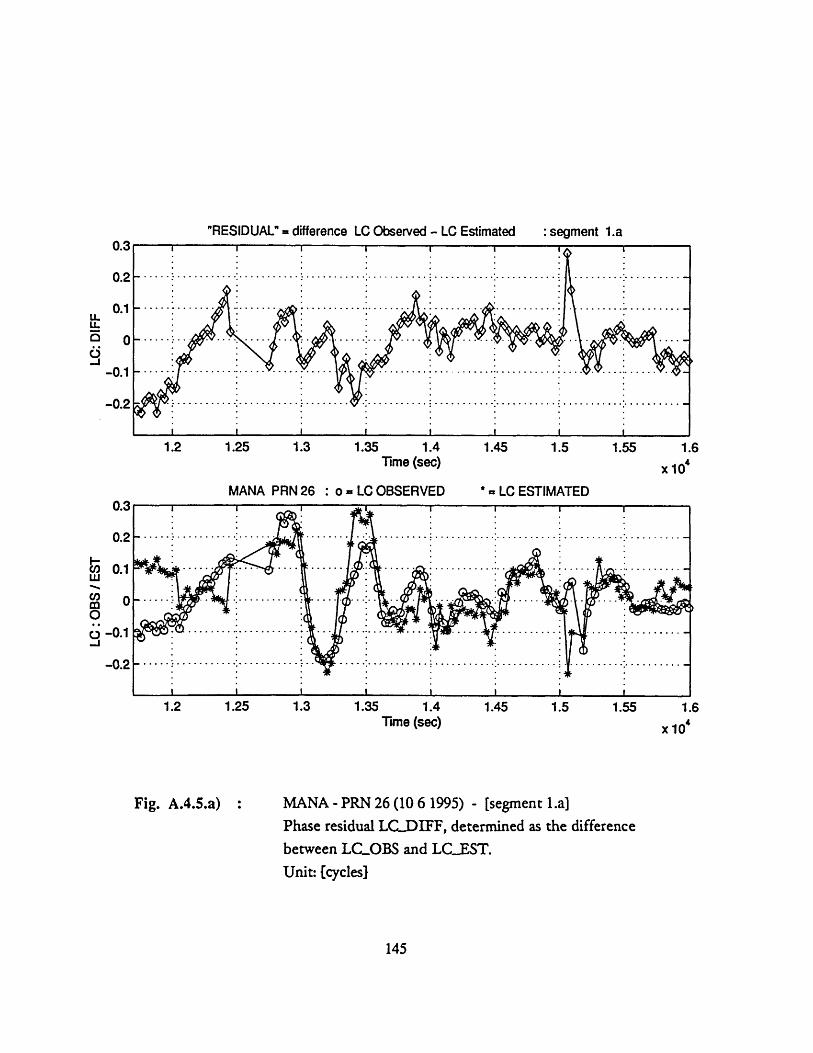
"RESIDUAL" = difference LC Observed - LC Estimated
1.2 1.25 1.3 1.35 1.4 1.45 1.5 1.55
Time (sec) x 10
MANA PRN 26 : o = LC OBSERVED * - LC ESTIMATED
1.2 1.25 1.3 1.35 1.4 1.45 1.5 1.55 1.6Time (sec) x 10'
Fig. A.4.5.a) : MANA - PRN 26 (10 6 1995) - [segment 1.a]Phase residual LC..DIFF, determined as the differencebetween LCOBS and LC.EST.Unit: [cycles]
145
:segment 1.a
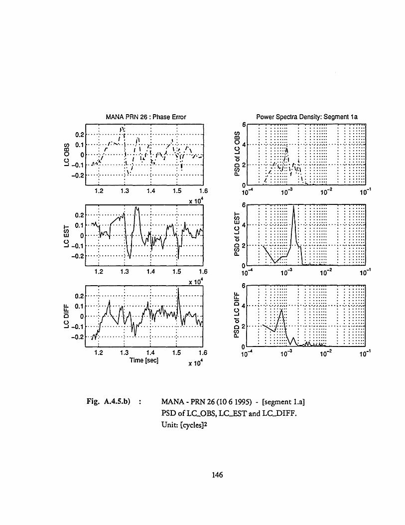
" ......~. ...........
.......-.............
.. ..
:. .
......-. .
..... .
............
.,
.. .
... •..... ..
,
...... .......
......
.......;......"...:..."
:::: ::: :::
::: :::
L
.. ·....
[ ....
.t ,%
. .
.....
:. .... ? ..:,•
$801t J o
Sd
S130 01 10 OSd
: *
.*
.
ICSBO
01
...
..
..
.
...... ......
.....
..................
... .........
......
.....................
.......o............
.......
..
...
.....
Ig
CO
v
C03
OC
IS30110 OOSd
.I.
wD
1t C
0 0>
ziO
01
jo aS
d
.IS3 013
..,. .,.. ...... ...t ..
....
.......... ... • ......
...... ....... ......
.. ...
..,, ..
., ...,b,.
:.:.::::--;---.......... •
. ......
..
....... -...... ....
• ~...·
.·...••.
.,.
..
,, :
:·
·
UV
)
E1=
I I
:1=10 0-1
Cd
cUu
v
r("
.o
1I
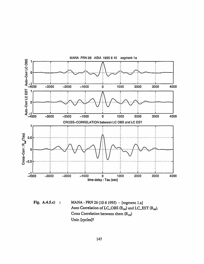
MANA PRN 26 ASIA 1995 6 10 segment la
-3000 -2000 -1000 2000 3000
1000
CROSS-CORRELATION between LC OBS and LC ESTI I I I
, . ........... .°. ... . . .
I I......
-3000 -2000 -1000
Fig. A.4.5.c)
time delay :Tau (sec)1000 2000 3000
: MANA - PRN 26 (10 6 1995) - [segment 1.a]Auto Correlation of LC_OBS (Roo) and LC...EST (Re).Cross Correlation between them (Roe)Unit: [cycles] 2
147
co0C.)0-j
-1-400
-404 4000
0.5
-0.5
-1-4000 4000
00 3000
30
2000
--- °°°

Cohe
renc
e0
0 0
p-
, 6 -
_
AMPL
ITU
DE
of S
O(f
)o
> (D
C
) C
)C
O
C>
C>
Co
o 0
0
LC O
BS /
LC E
ST
-A C I .
C)
(D
r-3
Nv a
S (f
) and
S
(f)
.&
is,
C)
C)
C) ~
o 0
0o
0
0
(D ~Cl)
(D xj 0
<01
i'
S-L
r C
A
.L
:3 0 0 0 0c t-4
.a...
......
...
....
..
.
........
..
....
...
....
...
. ..
.i ..
.. .
..... ..
...........
..,
r ;
.,
.. .
....
..
..
... .
... ...
.:..
....
....
....
.
.......
:....... :
.......
;...
... .
.'.'. .'.'.'..
'.. '........
I ...
..
:::::::::::::::::::::::::::i
....
....
--
•..
...
..............
..
................
...
....
... .. ..
.ý7
-
............
.. .. .. .. .. .. .. .
......
... ..
......
......
......
t..
.. ... . .......
...
I .....
..::'
::; ::
m
i I
E
IA
MPI
TDEo
fS^(
l
****
°,, ..
..°.
.........
...
o....
..
.... .
..
.a. .,
, .
, °....,
..
...
... •.
......?
....... :
....
..
...... ;.
.....
...
...
3 ...... :.
....
..............
··~
·......... ...... ......·
....................
....
....
....
......
......
..'··· ·.
·""..........
3hL
......
....

"RESIDUAL" = difference LC Observed - LC Estimated
1.6 1.65 1.7 1.75 1.8 1.85 1.9 1.95 2 2.05Time (sec) x 10'
MANA PRN 26 : o= LC OBSERVED * = LC ESTIMATED
1.6 1.65 1.7 1.75 1.8 1.85 1.9 1.95 2 2.05Time (sec) x 10"
Fig. A.4.6.a) : MANA - PRN 26 (10 6 1995) - [segment 1.b]Phase residual LC..DIFF, determined as the differencebetween LCOBS and LC.EST.Unit: [cycles]
149
LLLL53ej
w0,CD0
O-J
: segment 1.b
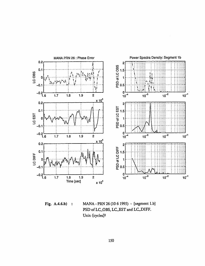
............ . ** **
......................
...... .....
•.....:11 el i I
:i I
j I !• !
i I I
.... ... .
.
::! ...
................-....~ .',...t...
,., ...~....
•
... •,. e..•
,.o..
.,........~
,. #,..
q,
• •
• •
.,,
-"
•~. ..~.. ....
•- .
.:. .
07-
S 0
SGO
01 0o OSd
-a
c~co* .-.............
a-q'I-'
a).,.-...
...-....
Co
•:. C
-
,
O.O..I. .... .
S.,•_•
00O
1(U
•-
0
r (M•'"
SB
0"1;
....... .......... ....
r- oC)
I .
.o
N
V-
0 -7
IS3 01
C
r- 0
-
-I10 01
...
.....
....
... ..eo
i
...
...
.
.......:..... ...... ! .
.... .
.... .
... ..
.e
..0
...... ....
...... ......
,o .
.o.
...
..
.
.. .
o
.......
...
...
.. ..
...
• •
.,. ,
• ,o •• •. •,
w••
::: ::::::
:::
:::
::
C
14 ') L
O 0C
V-:
C;
:: IO7
1o (1O
Sd
:EI--4
Q)I'U
-0
V/
P.,
as
oo E
7 -
co
I
I'I,rh
,,
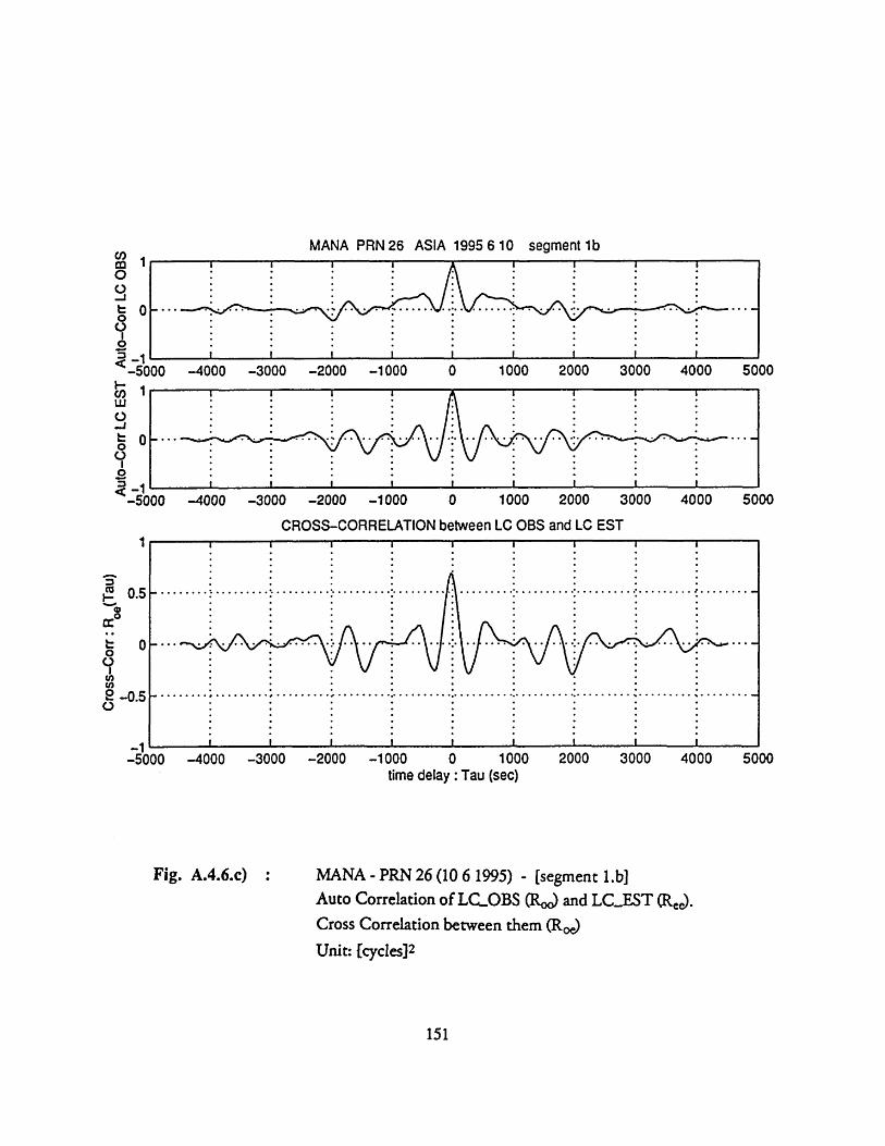
MANA PRN 26 ASIA 1995 6 10 seament lb
;i, 1w0-J
o
-4000 -3000 -2000 -1000
I-000 -4000 -3000 -2000 -1000I-5000 -4000 -3000 -2000 -1000
0 1000 2000 3000 4000 5000
0 1000 2000 3000 4000 5000
CROSS-CORRELATION between LC OBS and LC EST
0.5
0
-0.5
_1
-5000 -4000 -3000 -2000 -1000
Fig. A.4.6.c) :
0 1000 2000 3000 4000 5000time delay :Tau (sec)
MANA - PRN 26 (10 6 1995) - [segment 1.b]Auto Correlation of LC.OBS (Ro) and LC_.EST (Ree).Cross Correlation between them (Roe)Unit: [cycles] 2
151
c/)'niO
SO
oI
-50000C-)0
-5000I.-
I I I I I I I I I
I I I I
I I I I
ca
cc
0O,
L .A..0 .. . ................
I I I I ii,
i I i I i
.... ........... ...... . .... % . ..... .o.... °. ....... .. .......... . .......... ........
n~ i

0a.LCOI0.
90
0 0IS
3 01/ S8O 01
N
.....
0
......
... .... .
.,. ..... ....
..........
........"..
...... :.......{
.......•...... :......
.....~.
~ ~
..............
....... •.............,.. •...o........
...... ......
... ......
........................ .........
.................................
..
..
..
..
... .. .... ..
... ...
.. .
.. ..
.. .
.. ...
..
............ .
..... ....
: : : : ·:::...............'::·
.............
ii
...........
......
,......
.....
o o
0o
c0
0o
o0S
o ~o
o j~~
0 0
I I
-c
cr) *i
Gouejeto0
0
0O
0D~
ed ud qo
o%C)
o C
) C
.C3 P
C,
CJ)
(W
s p
ug ())S
CCLi D
...... ......
...... ..... : ......
...... :.......{
.......)...... :......
...... :.......•.......•.......:......
... ......
.......%
....... ..... .
...............,....
...
...
..
........
···
r......;......:.
.........
S............. .....................
o0oC)01I-
U0UC
)Q(
0C4J
C/)0
1A
q m
E
r
T-
€ i-r-i-r
4,
o v

MANA PRN26 - ASIA 1995610
... .....-..........:......... .............................. ... .............. ..i. ......
rll: 9lotI
.... .. .. .. .... .. .. .. ......... .. .... ... ........ ... ............. ....... ..... ........ .........
4.2 4.4 4.6 4.8 5 5.2 5.4 5.6Time (sec) x 10'
4.2 4.4 4.6Time (sec)
5.2 5.4 5.6
Fig. A.4.7 : Station: MANA - Satellite: PRN 26Data acquisition date 10 6 1995LCOBS and LCEST compared for t=4.1 - 5.8 10 3 secUnit: (cycles)
153
0.3
0.2
0.1
0
-0.1
-0.2
0.3
0.2
0.1
0
-0.1
-0.2
.............................................................. -
-4 -o. I. .~. r• : IW % I.- ... .:... , .., ...• .I,... .. : ....,.: . ../ .,i .. .v.. : "- ' : . : . r ' - - " : .· ..
!Ll i: I
x 10'
r
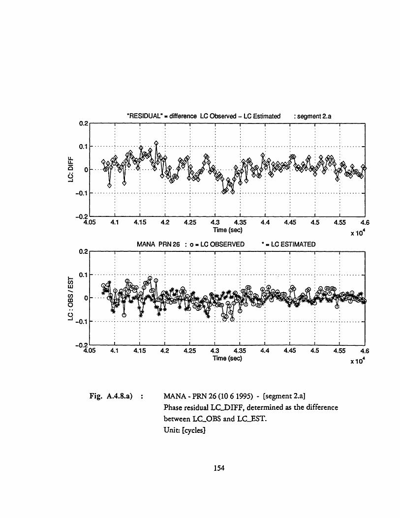
"RESIDUAL" = difference LC Observed - LC Estimated
4.1 4.15 4.2 4.25 4.3 4.35 4.4 4.45 4.5 4.55 4.6Time (sec) x 10'
MANA PRN26 : o = LC OBSERVED * = LC ESTIMATED
4.1 4.15 4.2 4.25 4.3 4.35 4.4 4.45 4.5 4.55 4.6Time (sec) x 10
Fig. A.4.8.a) : MANA - PRN 26 (10 6 1995) - [segment 2.a]Phase residual LCDIFF, determined as the differencebetween LCOBS and LCEST.Unit: [cycles]
154
0.2
0.1
-0.1
_n o4.05
0.2
-0.1
-n4.05
: segment 2.a
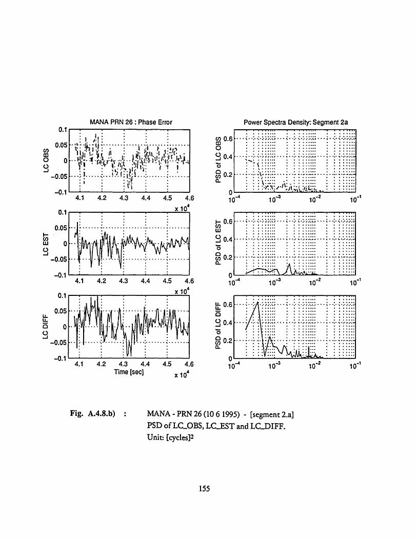
.......
.... .
..... ........
•.••••°°i .
°..........
...
....
: ..
....,
... .
... .
..
.... ...
~
Ico
D
o C
o
$80 0110
0Sd
.... : .....-..:..... .: ....
: " "-- • ;,,.,•
•-
:'•" i
e *
°
..... =•-'r.- .....,,.i .
•
o II
IS3
0-1 0
Sd
C
-
d o
O.
do
0 I
IS
90 0"
1
oD
V
Co
o
:--110 0"10 ]Sd
to o
mC9
40o
oI•~l:l
0"1
17C)
cdIcl~
i
C)
0o\C1
z
Or-
(O1=
V-
IndR
0
g
• |··
·T
L·
·
°°
°•
'.... ....
......
...........
...............
LS3 O-
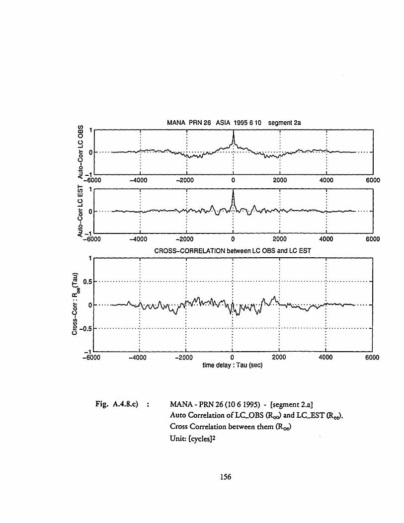
-4000
MANA PRN 26 ASIA 1995 6 10 segment 2a
Do 2000 4000
-4000 -2000 2000
6000
4000 6000
CROSS-CORRELATION between LC OBS and LC EST
-2000
. .' . . .
-4000 -2000 2000time delay : Tau (sec)
Fig. A.4.8.c) : MANA - PRN 26 (10 6 1995) - [segment 2.a]Auto Correlation of LCOBS (Roo) and LC..EST (Re).Cross Correlation between them (RO)Unit: [cycles] 2
156
cnlO0
-0oIo<-60
<-1
-60
. .. . . . . ... ..
I I I _ A _
-0.5
-t1
-600 )0
S... .. ..... ' ................. .............
4000 6000
00oo
00
2000 4000
.- °.°. °°. ° .. .. .. . .. .° .
.. .. . . . . . . . .
..... °°°
-

U)
0coIa-0M.
Cl
0,
o,,, ..
1..I,:-.1-.
,,:.....
::ii::::::::~i:::::::::::::: :::::::::
.......
·.·.
..... ...
.oe.
..... : .....
.....•.....,
.....•.....
.····.....·)·.·i·.
·.
··............
,.8....:.ll,
i·l
...'. .
....... .........
........
.....~~~
~~ .
..
..
.... .. .
..... ..
.
.. .. .....
...
..... ...
. ....
: .: :..
..,
,.....0,, ,o,
,.
.e ,.,,,
.... ..d .l.·'
.
...........................
... ../
o..:..:..: 0 0
0
0.:.:
,o LO
pu
( o(1) SP
U( O
) S
<oo
o L
IH
pm
O
ds
a ac
0
o an00
N1~
C?0
.s
O
O
O
O
O
C
(O
1 o)
C C
) C
/'d(1
)s o 10O
fhIndV'JV
I*L-I-C
O
Cd
O.-0
iE
LL
j0wzwccw
8j
00
Sco
c;oC
IS3 01 / SO
031
.. .
..
......
,·
....
r .....·.....
..........
ii I.........r.....·......
.....·.....
r..,........r.. ·
·.......:.....'. ........'..............
.. 8...
.. ..
....
..o..
..
..
..
,,,
.. .....
,.8
...-
...I..,.-..
,.
....~..
..
...:....
~~.
..... :
..
.
•
........ .1 ,,
.%..
,1. ...
+,%,
o
%4o
C,
oa
4
1U
0 40
o r
4-.
0u).4H,
eoueoeqoo
0
.o...............
.......
.*..
.
................... ....
... ....
..
.......
.. .......
... ..
...
.... ...
* ..
.... ..
....... ....
....*.*.*.*. *
.--.
::::::::::::::::::::::: ...
:···~··:::: :::::.::
::: ....
..... .. .
• ~
~ .,+,o,. ..°. .
.o ..
.o.. .
."
...
...
...:"
......:
...
..... .." '. -:%
* ........ .*
....
.... .......
..
..
i I
I m
m
i
ca
0,-
a
Ior

"RESIDUAL" = difference LC Observed - LC Estimated
4.9Time (sec)
MANA PRN 26 : o= LC OBSERVED * = LC ESTIMATED
4.6 4.7 4.8 4.9 5 5.1 5.2Time (sec)
Fig. A.4.9.a) : MANA - PRN 26 (10 6 1995) - [segment 2.b]Phase residual LC..DIFF, determined as the differencebetween LCOBS and LC.EST.Unit: [cycles]
158
4..4. 5 4.7I I a
5.3x 10⁴
5.3x 10'
0_L
: segment 2.b
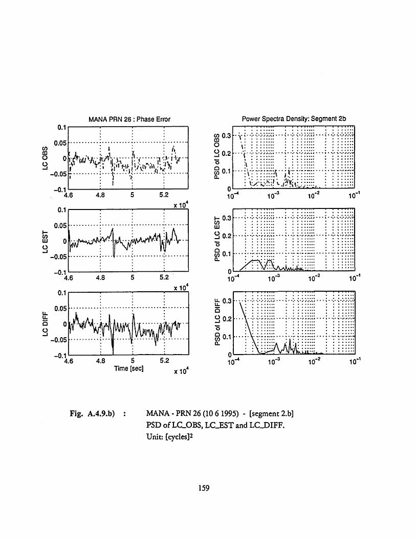
I-
m?
C>
-
.o
d o
SB
O 01J0 G
Sd
cuJ...
.-:,u
,_. .• '- -
L)
." .. R
~~cc
ci
) 0
) c
0 0 I
IS
G0 01
.... ....
..
..... 0
..... ....
...........
.....................
...............s......
............
........ ..
.... .
........
...... ...
........
...
...
"·
·,,··o
•
•·
...
*...
.. .....
.....
............... .....
...................**z
r .......
*,.o*
* .
..........."
CDC
-I
.....U
,...€
0 .
,
v,
I,c'J
i
~o,
.... .
.......
LOOR
-I-i0a O1
IC
V)
CO
0 0
IS3 01 JO G
Sd
........*..* ..
*....
.......*,.....
....
........o.....o
. ....
C>
..
...... .
.
.. .
y......... ...
..... ..
...
0.0.
.0
ddIO 0-1JO1
Sd-*
***
** :*
** :*
**-*
********
*********
-*******************
*
O
O
II
IS3 O1

MANA PRN 26 ASIA 1995 6 10 segment 2b
-6000 -4000 -2000 0 2000 4000 6000
-6000 -4000 -2000 0 2000 4000 6000
CROSS-CORRELATION between LC OBS and LC ESTI!
-I- · . .. . . . ..I I
-4000 -2000time delay :Tau (sec)
2000 4000 6000-6000
Fig. A.4.9.c) : MANA - PRN 26 (10 6 1995) - [segment 2.b]Auto Correlation of LC..OBS (Roo) and LCEST (Ra).Cross Correlation between them (Roe)Unit: tcycles]2
160
CCS
0
occo
o00
-1
1
0.5
0
I
,,-U.0 . . .. . . .. . ... .. . . . ... . . . . . . . .

Co C
o 0
o
1i) sPU
B (0) S
d o
0
0
1S3 0
1 /52
31
O
rLO
CV
001 09
n 0
0
( s jo 3O
fllldY4V
I-C)
[ucoS
C,)
E u-
p-OS
0cr3w00
0zwccwIa:00le
dIeouegeqOO
0
0
00
0U
J0
40
: ...
:.....~...
.........
."
1..........~........
..
..
...............
........ ............
~
.....'.... .
... .. ....
.. .. ... .
..
..
... .. .. .. .
.. .
.
.N
o
K
...
, .
-.
.....
.0". .. ...I., .
.. ..
..
..........
... ......
....... • ...
................... .............
........... ......
...... .
.....
"'
'!
...... :......
........:
...... •.....
.........
.....
, ,
.,
... .... ,.. ,
.:X :
···
···
···
··....
...
....
... .
...
... .
.. .. .. .. .
.. .
..
....
... ... ..
.... ... .
....
:.
... .2
·... ..
·;:........
... ....
..
*.
....
** * * * * *
**..
**.
**.
*
.......................... .......
: ......
::
~::* .:
: : : : :::: : :
.. .
..............
....~...~...:.......
.. .....
~
.. .
..... ..
*...... .
..... ..
... .....
·.....
.~ ....:..
...
.
J II
-o,-
q(cD V
.i

"RESIDUAL" = difference LC Observed - LC Estimated
5.35 5.4 5.45 5.5 5.55 5.6 5.65Time (sec)
MANA PRN 26 : o = LC OBSERVED * = LC ESTIMATED
5.3 5.35 5.4 5.45 5.5 5.55 5.6 5.65Time (sec)
5.7
x 104
Fig. A.4.10.a) : MANA - PRN 26 (10 6 1995) - [segment 2.c]Phase residual LC.DIFF, determined as the differencebetween LCLOBS and LCEST.Unit: [cycles]
162
-0.1
0n 2-v5.-.
5.3
wCLLm00
5.7x 10⁴
:segment 2.c
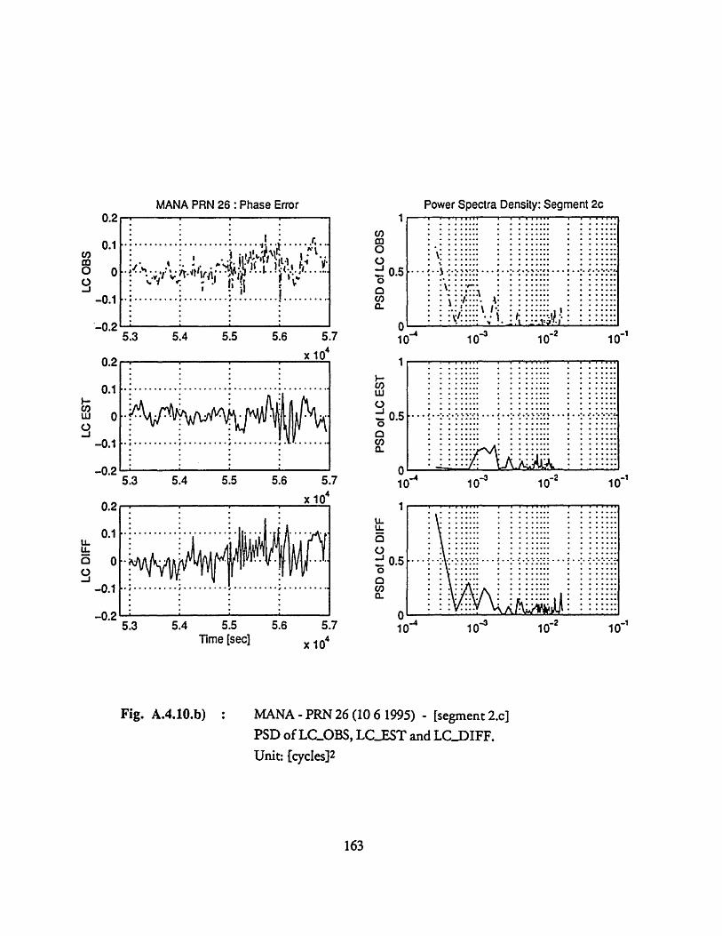
LC D
IFF
I I
o O
O
O
1..I+
..i,
ulr
ul :01 LT
I01 01
,I I
Cl
-L
0
-&
tu
i.
.. ..
* *
_
....
..--
i :
PSD
of L
C DI
FFo io
-
......
....
·····
.. .
.. .
..........s..
........
..........
' '''
..
...
.
O&
-I
I
.L 0
PSD
of L
C ES
T
.. .
..
.% .
..
..
.......... .
~.........
i.............
....... ..
.....~..
.. ..~
...
.........
...........
I
PSD
of L
C O
BS0
-'0
*0
-
'b1
0
..:.
....
......
...
...
.. ...
.. :.
..
. ..
.. .
..........
... ......
........
....
....
....
....
....
.......
...... ......
......
......
....
·...
..%
..
..
..
i( 01 :rP
2 CD
C,)
CD
X x , .. 0=
ci 0,
1 ·
""""
""""
"'"
····
·5···1
·····
LC O
BS
%0i
JL
I
I
LC E
ST
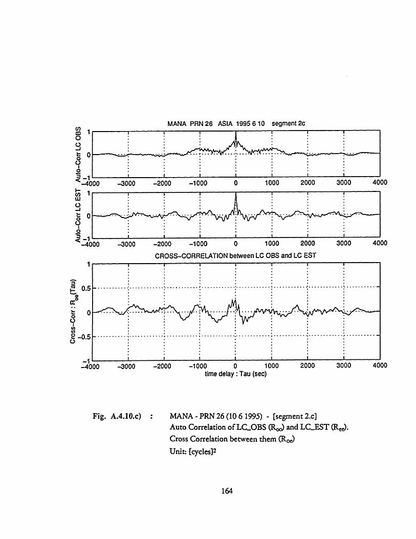
MANA PRN 26 ASIA 1995 6 10
-3000 -2000 -1000 1000 2000 3000
-3000 -2000 -1000 0 1000 2000 3000
CROSS-CORRELATION between LC OBS and LC EST
-2000 -1000time delay :Tau (sec)
Fig. A.4.10.c) MANA - PRN 26 (10 6 1995) - [segment 2.c]Auto Correlation of LCOBS (Roc) and LCEST ( .Cross Correlation between them (Roe)Unit: [cycles] 2
164
. .1 7.. .......~·· ~ ~ ·~~~·~~
00
t O
0Io
-40_
01
L-
0o
I-1
-40c
4000
4000
3.
oo
I
0
0.5
-0.5
4
-4000--.400 -3000
I I I I i
S............ ............ .......... ........... . ......... .. .. . ........... ........ . .........
,.....~~....... .·· · · · ~ · · · .....· · · · · ·. ••..--···-~ ~ ~ .
1 I _t 1 I I1000 2000 3000 4000
• ° • • • °
I i I I I I I
segment 2c
00
00
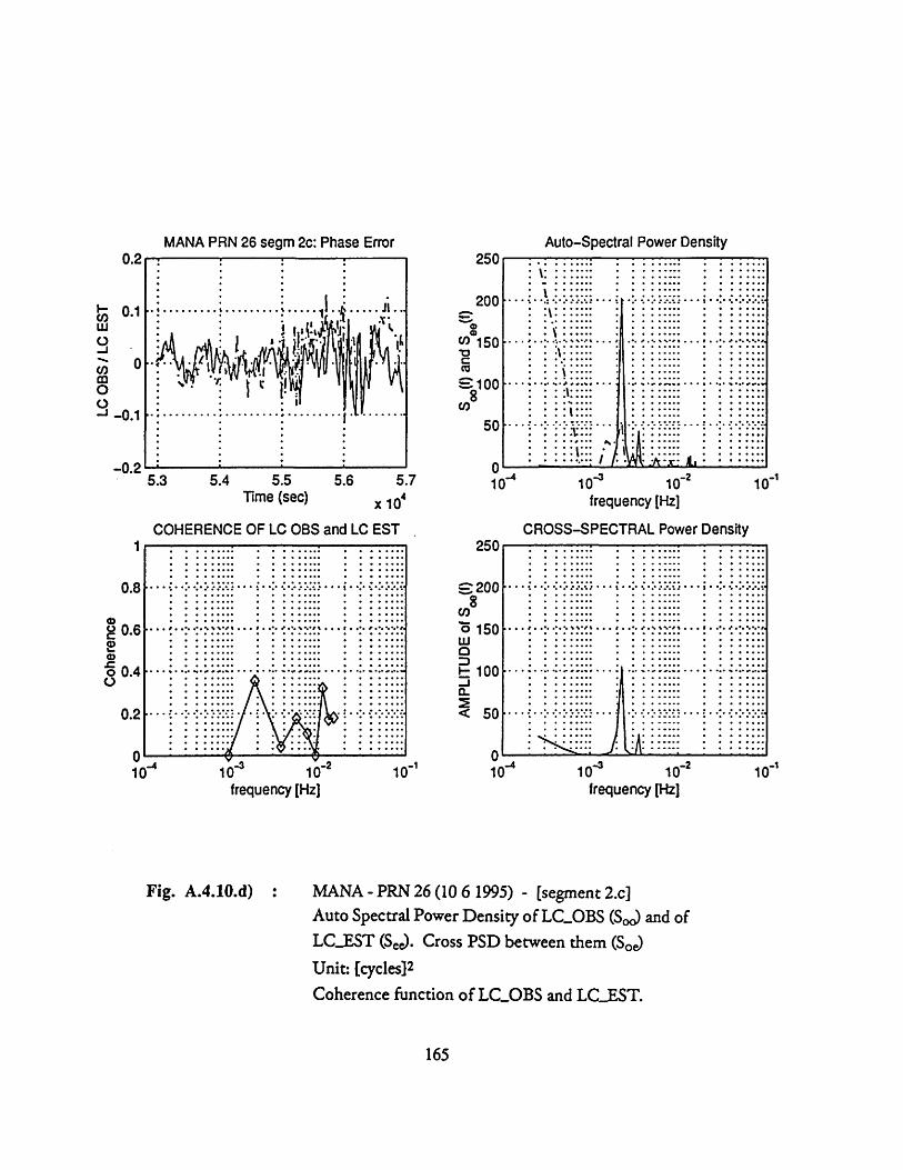
Coh
eren
ceo
0
0rP
,.P
P
0
LC O
BS/
LC E
ST
C1
--i 0**
b)
AM
PLIT
UD
E of
SO
(f)-A
-A
ro
m
r(1
0
0.
0 01
0 0>
0
0 0
-LC
U.,
.
O0
0 C)
n 0. Co S0 O laC
.0\ H
r
0 9
0 -&
SO(f)
and
See
()-L
-A
01
0 01
0
0
0
-A
o EC,
0 uQ
U' C,)
C,)
0n
0Ob
0, o Co
cc,
r1 U' 0
0 m0 C) 0 (0-u C) h =3
U-
0 CD 0 CD
cn
-LA k
....
.. ......
.... .. :,.. .......
.......... .......
....
:' "::.
..:::: .
..
...
:.:
....
.. .......
.......
....... : .......
....
.. ..
..... .
...... ..
....
: .....
.. .... ...... ............
2 .
......
...............
o
..
......
....
°°
°
.°
,€...........
.. ......
°,°°°.°..o
,.........
, •
.,
.....
o.. ..
..
?:!?
90 9012 60
130
18 ....,... .* . .. .
21 0
240 •300270
receiver location: CENTRAL ASIA acquisition date: 10 6 1995
satellite: PRN 284UU
o 300I
200
100
n
0 2 4 6 8 10Time (sec) v n 4
Fig. A.5.1 :
station: MANA
0
satelite: PRN 28
2 4 6 8 10Time (sec) x 10'
Satellite visibility chart for PRN 28 (skymap).Elevation and azimuth of PRN 28 with respect tothe station MANA
166
GPS DATA:
station: MANA·IAl
4% IV

MANA PRN 28 10 6 1995
1 2 3 4 5 6 7 8
Signal to Noise Ratio for L1 and L2
Time (sec)
Fig. A.5.2 : Station: MANA - Satellite: PRN 28Data acquisition date 10 6 1995Signal-to-Noise-Ratio (SNR) for LI and Lz.
167
I
.ocaC.2
w
0 9x 10'
4UU
-J
cc 200zCO,
'4UU
200
0
9
x 104
_ _
N ........ ............ ............ ........... . . . . . . . . . . . . . . . . .
..... ... ....... .......I I I I I I 1 I
,,
t
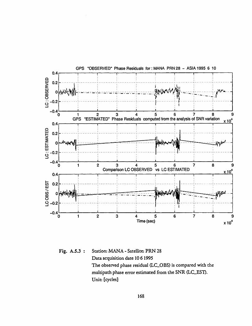
GPS "OBSERVED" Phase Residuals for: MANA PRN 28 - ASIA 1995 6 100.4
L 0.2
. -0.2
-0.40 1 2 3 4 5 6 7 8 9
GPS "ESTIMATED" Phase Residuals computed from the analysis of SNR variation x 104U.4
w 0.2
0-0.2
U.4
C 0.2
C/) 00
O- -0.2
04J
0 1 2 3 4 5 6 7 8 9Comparison LC OBSERVED vs LC ESTIMATED x 10
0 1 2 3 4 5 6 7 8 9Time (sec) x 104
Fig. A.5.3 : Station: MANA - Satellite: PRN 28Data acquisition date 10 6 1995The observed phase residual (LCOBS) is compared with themultipath phase error estimated from the SNR (LCEST).Unit: [cycles]
168
I B I B B B I I
S. . . .
! . I
-- -.1
·,-.- ·-, · ·--- i I i i
~1

MANA PRN 28 - ASIA 1995 6 10 :segment #1
1000 2000 3000 4000 5000 6000 7000 8000 9000Time (sec)
1000 2000 3000 4000 5000 6000 7000 8000 9000Tine (sec)
Fig. A.5.4 : Station: MANA - Satellite: PRN 28Data acquisition date 10 6 1995LCOBS and LCEST compared for t-0.0 - 0.9 10 4 secUnit- [cycles]
169
0.2
n -U.'
02
0
0.2
0.15
a 0.1wa 0.05
00
6 -0.05
-0.1
I I ~ - I I I I I
..........
.................V...
It'.
i - I01C
0
,,
. . I i I . i
c
I

"RESIDUAL" = difference LC Observed - LC Estimated
1000 2000 3000 4000 5000 6000 7000 8000 9000Time (sec)
MANA PRN 28 : o= LC OBSERVED
0 1000
*= LC ESTIMATED
2000 3000 4000 5000 6000 7000 8000 9000Time (sec)
MANA - PRN 28 (10 6 1995) - [segment #1]
Phase residual LC.DIFF, determined as the difference
between LC.OBS and LCEST.Unit: [cycles]
170
Fig. A.5.5
: segment #1
--
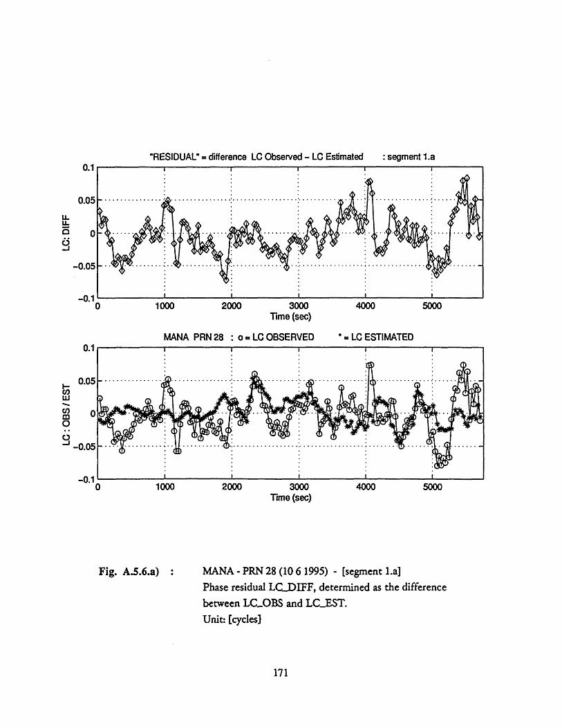
"RESIDUAL" = difference LC Observed - LC Estimated
0 1000 2000 3000 4000 5000Time (sec)
MANA PRN28 : o= LC OBSERVED * = LC ESTIMATED
0 1000 2000 3000 4000 5000Time (sec)
Fig. A.5.6.a) : MANA - PRN 28 (10 6 1995) - [segment 1.a]Phase residual LC.DIFF, determined as the differencebetween LC.OBS and LCEST.Unit: [cycles]
171
-,. I
: segment 1.a

S80 01 lo0 aSd
o0Co
: ,. '-- " ;
*Iz .
.0
* ".•
•
."
-o:
I) io
o
I!
...o. .. ...° .o. .°
..
.., ..o.
:::::: ::: ::: ::::::
....,...,....·.......
..
.. ...... .". .
• .-..
..-
... .
: .-...
.-.-
: *
....
... :...
....
..i
.-.. -.
."
...-
.........•...........
•· ·
··
··
:· ·
,,••••
%,...
•'
··
·~···~· .,···
.,.·
··
: I...
··..
.°°
.,
• .. ..~.. .
... :....
:....
•
•
,
•
.|,·U~
c
IS3 010o O
Sd
oC>
oo
In00
,.......Z..,...........
::::i:::j::::·::::::::::
.. .... .
... ..
..... .
• .... ..
.......
..... •....
.... :. .
.
...................•.
...•...•...
····
:
: .•··
0 00
JAM
0110 GSd
,- L
n
•o
oI
S 11la 0"
I
C4"U
~
0
6y-
I
...•
......... ....
..
.........
.. ...
.... ..
:...
...... .
..
·
...; ... .
...
1. 1 ...
• ...
IT
7'
8O
0"I1
83
0"

MANA PRN 28 ASIA 1995 6 10 segment la
2000 4000
00
-0UUU
-4000
-4000
-2000
-2000 2000 4000
CROSS-CORRELATION between LC OBS and LC EST
0.5
.. .. • ,,,, ,, ° °_................_
time delay: Tau (sec)
____________I-- _________________
2000 4000 6000
Fig. A.5.6.c) : MANA - PRN 28 (10 6 1995) - [segment 1.a]Auto Correlation of LC..OBS (Roo) and LC.EST ().Cross Correlation between them (R,)
Unit: [cycles] 2
173
Cl,
O0
00
0OSO<-1
-60
I I I· I IL· V-~· ~·· · · · · \- l-V · ~·· ~ ~ . ~ ·
1
6000
I II I I
6000
-0.5
_1
-6000 -4000 -2000
. .!- : - - - - - - -
2000 4000
-- L
-...... .. .................
'': ~r~y· ~ ~ I '~ '' I ''I'.' \'''~/ ~'''''r 'r ''/ ~''Y''''''L.'''
. .........

o 00
oo
0
0
() S pue ()
S
O
O
O
O
C0
0 0
0IV
C
l) C
W
¶
(09 0S 1o 3aflhndV4dV
d ;
O
d0eG
aJeq00IS3 0" / SO
O 31
...........
S
.......
...
.(...............
..... .....
......
.. ...................
...............
..
...
....
..8..
....
... .
...
..........
..........
8.........
............
...~........
......'.
.... .. .. ..
............................
IVw
(I)
'I-
0%C'
00ooo(•!
0oI
I
m0
0 0
0 C
0 0
0 0
(1) S Io 3C]rLl.l-ldiAIV
........: .o.
€...
,,%
......
.! ... ..
...
.•o
, ....•o
.,
........
.. ...
..
.,,,,°*o.•............o
$
.o.
oo. .
......o.o
....o.......
..
....... :......
...... ....... :......
c o:)r-
(o

"RESIDUAL" = difference LC Observed - LC Estimated
7000 7500Time (sec)
MANA PRN 28 : o = LC OBSERVED * = LC ESTIMATED
6000 6500 7000 7500 8000 8500Time (sec)
Fig. A.5.7.a) MANA - PRN 28 (10 6 1995) - [segment 1.b]Phase residual LCDIFF, determined as the differencebetween LC.OBS and LC.EST.Unit: [cycles)
175
0-
.1 --0
-0
I I II-
9
6000 6500 8000 8500
I I 1 1 1 1 1 I
I
: segment 1.b
..
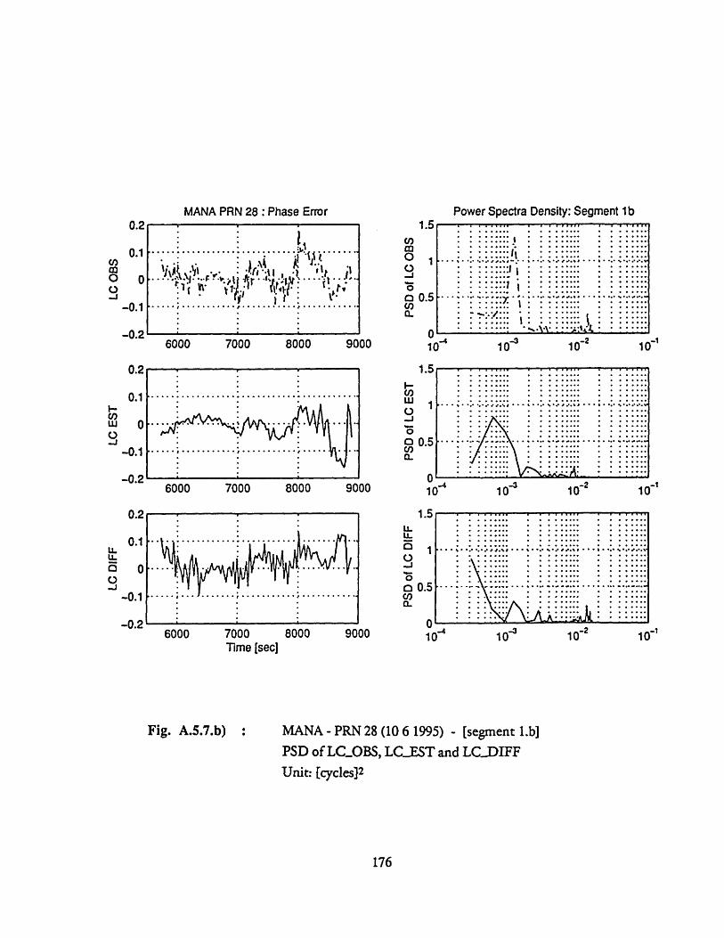
...
'.......
..................
... .
.. ..... ...
.: .. .. ...
.......,. ...............
.I .
.-. .- .
······i······:······
.. .. .. ..
o.
.... ..;
.. ....
•. ...
...
..
.. ..
.oo
I...,,
o::
i ....
..•
...... .
....... -...
...:
..,..,
,..... .o
.. .
--- -- -- A
LO
-In
CI:
0SBO
01 o O
Sd
-O
Sd-IS
3 0110OSd
............. .....
.
.. ... ......
........, .2.o•.
...
•.,
o
°
...... .
....... ......
.. ..
.... .
..
......* .............
.......;,......
...................
......
......
o
... ..+
., .
+
,S
o..
..
..
..
...........
.1 7
Ln
JJCI 0
10
o S
d
• .-,..
a'~
.- :
: :t.•
•
Y
, ..
·-C
'• ..
• •.,o.
.•
,
:
:':.,,-
: •.•'
.:_
•.
: " _..
N
T-
O
T-
N
I I
J-4l0 001
0
cu
1001r
PI
I
1 ·
IS3 0
1
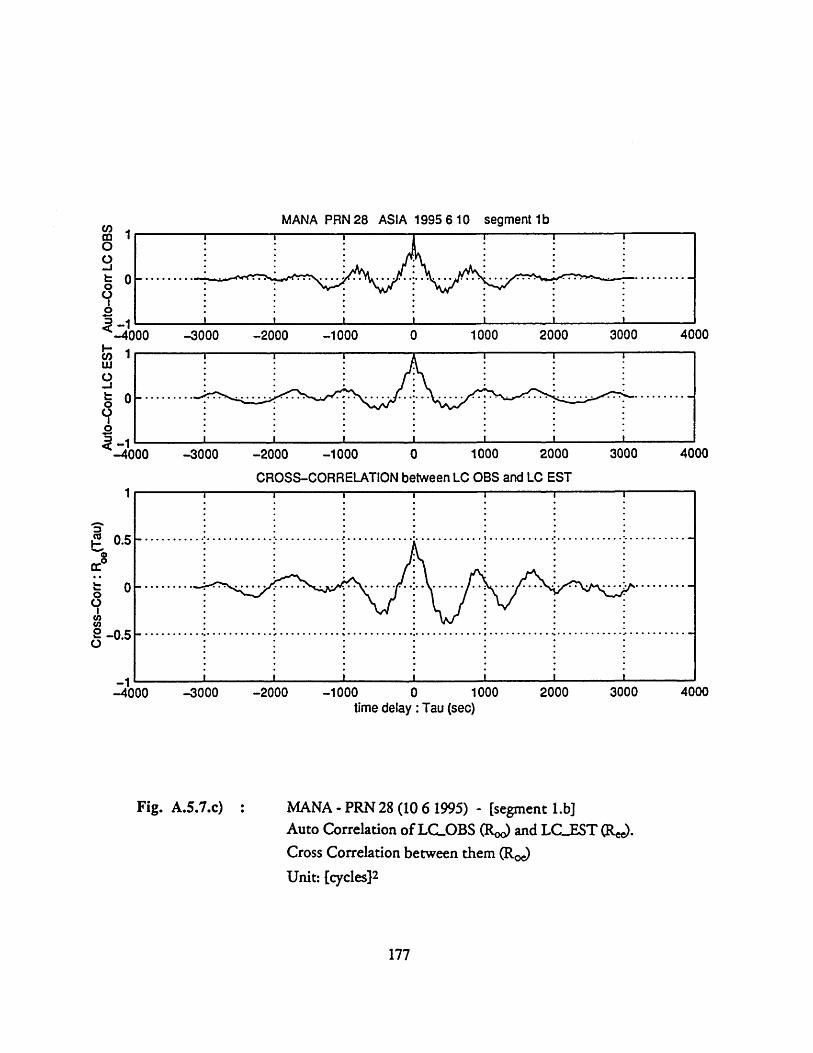
MANA PRN 28 ASIA 1995 6 10 segment lb
-3000 -2000 -1000 0 1000 2000 3000
-3000 -2000 -1000 1000 2000 3000
CROSS-CORRELATION between LC OBS and LC EST
-3000 -2000
Fig. A.5.7.c)
-1000time delay :Tau (sec)
1000 2000 3000
MANA - PRN 28 (10 6 1995) - [segment 1.b]Auto Correlation of LC.OBS (Ro) and LC.EST (Re).Cross Correlation between them (R,)
Unit: [cycles] 2
177
U,moO0tO-Jk 0
I
o 1
-4000LUw
oto
I0
Q- I-400UU
4000
4000
0.5
-0.5
_1
I I I I I S I
;.''''' · · ·; · · ·r··· · ·;.· · · · ··, ;'''' · c· · · ·
-40C 4000
.°.°o°°..
. ...... °°
)0
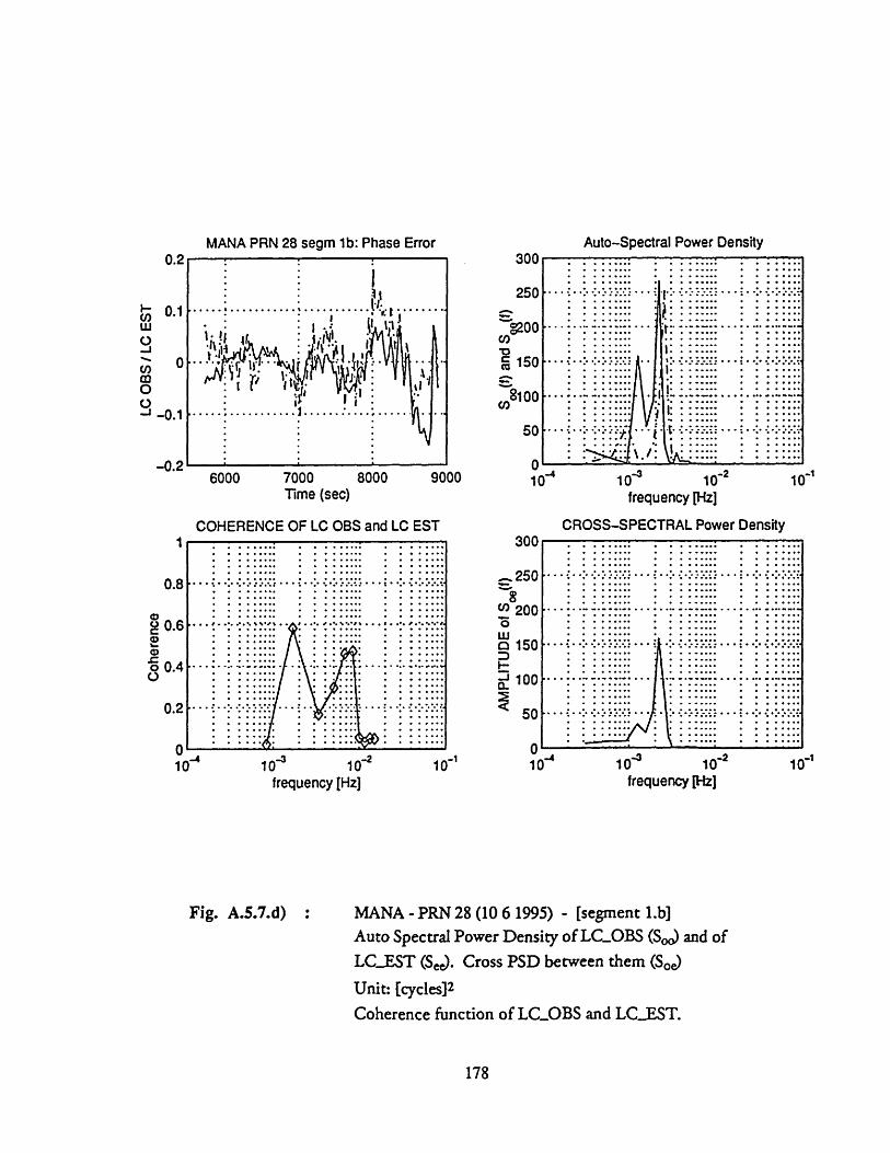
Cohe
renc
e0o
O
0
0=i ,
o.
b co
AM
PLIT
UD
E of
SO
(f)-L
-
0A
6
6C
) (n
l
(n
C
LC O
BS /
LC
EST
-.o
o\
So(f
) an
d S
(1
)01
0
0(1
0JC
) 0
0
0 0
•c
c) 0 :31
0 :3
c-0
00
:
-A
Ca
-L =%
....
...................
....
...
,..o.,,
............
...
*
..
...
*,
....
.. ..
..
......
• ..
.... ....
...
*.. ..
**
......
...
•
,
o,,
.,
"'*'**,**
' ...... .
...... *,. .,*...
.. ..... ..
....
.
......
".. ....
'···"
y·_·
··.
.......
..··
......
..
....
. ..
...
..
......
...
...
..........
..............
°..
...........
o..°..,
,.
.o°.
.. ...
,.
..... ..
..
.. ...
....
..
....
....
;.
.........
..
..... ..
.. .
..
.* .. .
...
..
..
.. .
....:.
..,.
. •.
.....
..
: ..
...
: ......
...
°..t......°*.°,°°,o
....
. i ...
..
I ..
...
; :.
.~~.
.. ...
...
.,,
._
V
L
:>
Ir
.. ....
....
. ...........
.......
....
....
..: : :::: : ::: :: :: : ::::
:....:
' .....
,.
.. .... ...
..
° .
...
•.
...
...
...
:* * I *
** I*:*I ::
............
oolO.oalO.oeol...,
·o.oooeo...•o•..
II: ::::::::::::::::::
::::::::::::
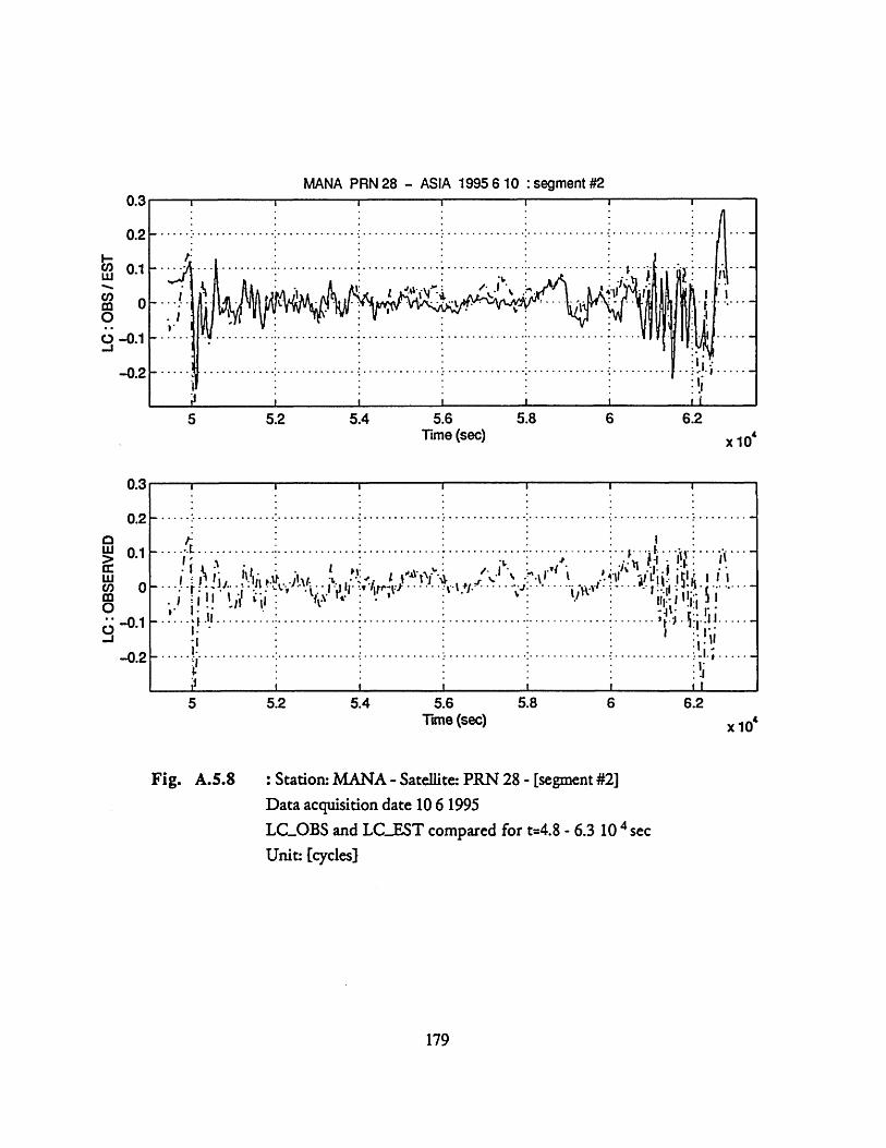
MANA PRN 28 - ASIA 1995 6 10 :segment #2
5 5.2 5.4 5.6 5.8 6 6.2Time (sec) x 10
5.2 5.4 5.6Time (sec)
5.8 6.2
x 10'
Fig. A.5.8 : Station: MANA -Satellite: PRN 28 - [segment #2]Data acquisition date 10 6 1995LC_OBS and LCEST compared for t=4.8 - 6.3 10 4secUnit: [cycles]
179
.. I I. . . . . . . . . . . .
..... : /- .A
• °~
11t tt___ *1r
0.3
0.2
0.1
0
-0.1
-0.2
A,
0.2
0.1
0
-0.1
-0.2
.... .. .. .. .. .. .. ...... .. .. .. .. .... .. .. .. .. .. .. . ... .. .. .. ............ ..... .. .. ... ..." .. .... .t .i ... ...
.. .i •l . .... .......... ...... ...... .......... .. ....... ........... ....... .. ....... 'J . • ..• iIl
I
I I I '"i.. ... . i I : l_
. . . ......... ... .. I' ......
r :,.fr
.. . . . . . .. . . .. . . .. . . . ... . .. . . . . .. . . . ... . .. . . . . .. 1.1
r
-4
· · · · · ·
it...... ...
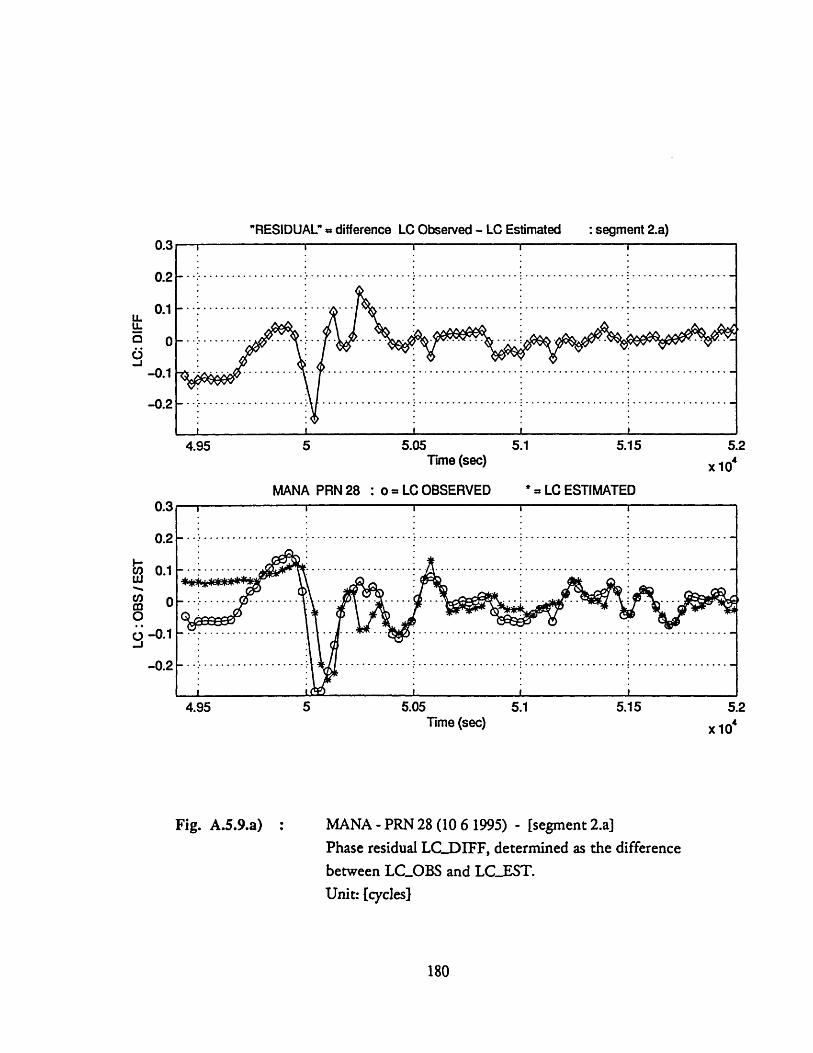
"RESIDUAL" = difference LC Observed - LC Estimated
4.95 5 5.05 5.1 5.15Time (sec)
MANA PRN 28 : o= LC OBSERVED *= LC ESTIMATED
4.95 5 5.05 5.1 5.15Time (sec)
5.2
xl0'
Fig. A.5.9.a) : MANA - PRN 28 (10 6 1995) - [segment 2.a]Phase residual LC.DIFF, determined as the differencebetween LCOBS and LC..EST.Unit: [cycles]
180
0.3
0.2
Co 0.1
0
y -0.1
-0.2
5.2x 10⁴
: segment 2.a),,
m
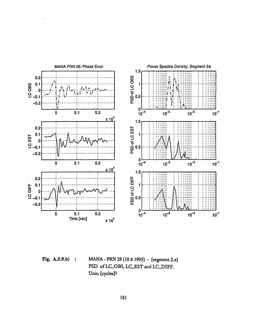
........,......,......
......,.'..............
.." .... ." ..
-.. ..
............
..... ° .
.° ........
°...
.......:,.......?....."..
0
C
-- 1
-O
)
S80"
1 o O
Sd
* *
-I.
..
• •
.... ... .. .: ..' .
.. :..
• • ,,,•
,
............... ......
.....o..
...
...
.....
..
... .
.. ...
..s
..
...
..
... ...
.....
..............
.....
S...
..
...
..
3r-o aS
c
IS~30110 Sd
No V
ac'-0
ci00C
I
I I
.............
......
•
... ..
...
...
..
..
.. .o.
....... ........
.............. e
..
. .. .. . .
. . ..
... . .
.
.........
,.
.... .. .
......·
··
··
··
·.. ...
.°......r ...
...... ;......
;.....
-lO 0
10o
OSd
C4-
[-,
9u04
n,
j r4-4I0;
z
i)
F:
ui
1IG0 301
II
I,
: :
:
.. .
·\··
2·• :
;
: :
:
,·
··~·
·\·°
: ."
• .
.
IS3 0
7

MANA PRN 28 ASIA 1995 6 10 segment 2a
-1000 1000 2000
CROSS-CORRELATION between LC OBS and LC EST.... I
-1000time delay :Tau (sec)
1000 2000
Fig. A.5.9.c) : MANA - PRN 28 (10 6 1995) - [segment 2.a]Auto Correlation of LCOBS (Roo) and LCEST (Ree).Cross Correlation between them (Roe)Unit: [cycles]2
182
co
-J
I-U) 1
0
-1J
-30( -2000I I I I ..
1
0.5
oo
2 -0.5o
_1
3000
I...............
-30( 00 -2000 3000
r-
L-00
fnV) I -
7
4 -
... ....... ...

C0() s pue (1) S
)o
uc r
O
-I I
iS3 011S80 0i
0 0
0 0
0 0
(ID
to o
1j/n-d
WOO S
1o3anfl.ltdYW
--
x W
S u
E
U
P
0wOcr
eougieqoo
•. •.. :.••
1....••,.... ......
...
S....% ..•.I.•...••.
..=
.......
...... ..
... .
........ .....
....
...... ...:.......
....
:...........................
.....
""'1"""""' ""!""·
:::::X:::::::: :::::::
:: ::: ::::
.....*..
.......
... n
.....*.....
..............
·........
·.
..
....
•.°••
• I.
.°....I•
••..
•********.*****t*****.*****t*****.****
.................... ........... ..
... .. ... .. ... ...
......
.
U/)
E0
C,
aCo00a-o0.C
,)0
cu'c
(..4
U;
NC0)
4?70
C1r
:.... ...
....
...
··
··
·~ ~
~ *
*- ~
*-r..- .
II I
I I
I
.......*......
.*...
... .
.........
:::: ::
:::::::::::::*****..
.:::
:::::::::::::::::::::::::::::::::::
...... ......
..... ..
... ..
.. ............
*...... .
..... .
... ......
o
o
o o::
:: ::
:: .
...
..,.::.
:::::::::::: ::::::
.. ..........
%**
*.
**
..
...
••.
***
..
4... •.........
...
:: :::::::;::::::;:fiC':::
: : ": :
... .
....
... .. .." .......
•...... : ......
...
..
.o -- * ..
.... .. .. ..
..
i •
I
n
tDoT
IOS
d L
_
01
C
--
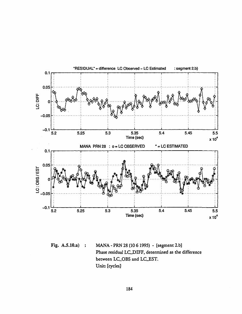
"RESIDUAL" = difference LC Observed - LC Estimated
5.25 5.3 5.35Time (sec)
5.4 5.45
MANA PRN 28 : o = LC OBSERVED * = LC ESTIMATED
5.2 5.25 5.3 5.35 5.4 5.45 5.5Time (sec) x 10'
Fig. A.5.10.a) MANA - PRN 28 (10 6 1995) - [segment 2.b]Phase residual LC.DIFF, determined as the differencebetween LC.OBS and LCEST.Unit: [cycles]
184
0.1
A A
0.0
-0.0
-0.1
I I I I I
5.2 5.5x 10'
i I
: segment 2.b)
I

... .'
...
...
.....
.....
........ ..
.. .... .... .... ...
.. .......
........
*...
... I......
....
.. ..
..
.
I_
S0
110o OSd
S---..........
........... .
'- C
0
d o 0
L)
CU
ui
.. .........:::::
::
.. ....
..o
..... ..
...
.... ....
... .
·~~~~~~1.::::1 "::1::
.,.....,.oL
*********
...............I....,
.... ...........
... .
Cd c
IS3 3110 O
Sd
c'J
U)
Ii-
=l1O 30 lo O
Sd
1S3 01
*.*
**.. ..
*. .
.-o
o-
o:*:
**::::: *:::: *:::::
**.*
*****:*
****r*
****
• :...... ? ..... .
..
**.*
... ***.*
*
..
..
..
....
..........
* *****····:······
***
*-*
**
**
***********·
**
:**
**
**
*
**
**
?*
**
**
**.*
*****
*****r*
****
********
***********··
** **
* *****L
*****·I· ·
=1-110 01880 0
"I
707-
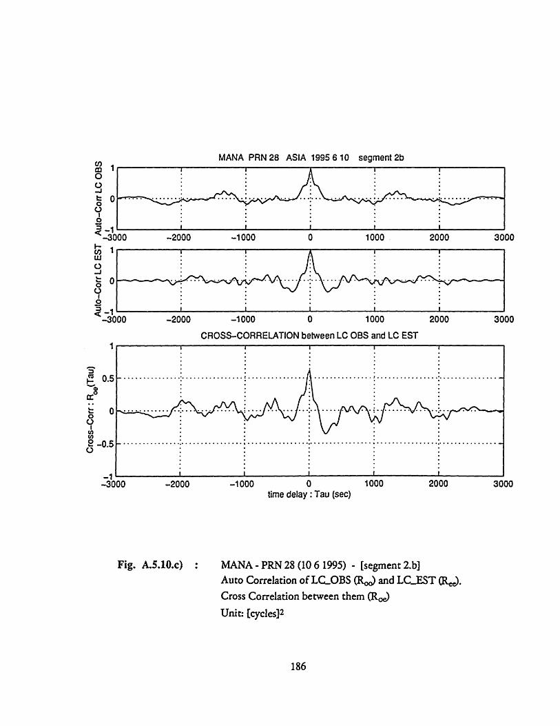
MANA PRN 28 ASIA 1995 6 10
-2000 -1000 0 1000 2000
CROSS-CORRELATION between LC OBS and LC EST
............ ............... .................
.. ............... ... . ........... ...... . .. .. ..
-2000 -1000time delay :Tau (sec)
I I
1000 2000
Fig. A.5.10.c) MANA - PRN 28 (10 6 1995) - [segment 2.b]Auto Correlation of LCOBS (Roo) and LCEST (R).Cross Correlation between them (Roe)
Unit: [cycles] 2
186
Oo.-
0o2Or<r
I.--
-oLUo
0o!
-3000
. 0
0o
2 -0.5
3000
_1-3000-3000 3000
segment 2bfnV) I -
................ .... ......
L-

C0U)I0a.
u,0
o o0
0tn
O
in
0(Ul
o ue
Of)'s pue (WOOS
-aio
o inI
.o.,,.o
...
...........
............ .......
....... ......
..
...
.... .
........ .....
....... ....
..... ....
, .
.
..
::::::.:::::.::::: :
inin.q*
ui
ui
....
*....
-..
*.........
..-
• •
o
o··
··
··
o 0
00 C
oo on
0C
o
m
1
Y
(I)"S 0o 3OflhIndV4V
Ce ueCeq
GO~uojiOLO
ICo
IS3 0
/ SB
O 01
I_
NC1r
2-1v
............ ....................
..
..
..
..
..i....
.......... ......
;............
......:......
......
........ ..
!.
...
:.
.... ..: :
• •
.o
II
I
I
I
..
... ........
....... ...•
i·· ·····
oC>
...
*.
....
...
O,-
-----
--t
o0 T-

"RESIDUAL" = difference LC Observed - LC Estimated
5.5 5.55 5.6 5.65 5.7 5.75 5.8 5.85 5.9 5.95Time (sec)
MANA PRN 28 : o= LC OBSERVED
6x 10'
*= LC ESTIMATED
5.5 5.55 5.6 5.65 5.7 5.75 5.8 5.85 5.9 5.95Time (sec)
Fig. A.5.11.a) : MANA - PRN 28 (10 6 1995) - [segment 2.c]Phase residual LC.DIFF, determined as the differencebetween LC.OBS and LC..EST.Unit: [cycles]
188
6
x 104
: segment 2.c)

o80 30110 O
Sd
:::::::::::..............................%.......................
...o
.. o
...................
.................................................... .
.............................
L-
C
IS3 01 lo
Sd
...
,..,
..........
......... ..........
......... ..........
.........*..........
.,
° .
.o
..
..
• .
.o °.
,
!!....................
*** < * *
...
.......... ...................
.....
....
........... :.... ....
...
:.........
• .
.-, -..
:.' .... ...
":...
.i,.
...
4.-.
.". .
.'. .
.
K ..,? A,,.
U
7'I L
c; C;;
-U
) 0
U)
d o
o d
0
0
I
T-
ud
oo
S8
0 31
o U
)C
) LI18~3
0
o'J
uicoui
CD
U)
U)..
fLei
V-
0n
U)L
) V
-6
R.
R
cid
c o
:11G 31
..........*
* **
* .
..........**.........
....................
..........** **
*****.*...*****..***
............* ***
........*..........*.
I
: S
d
II•,-
u
r..
......
........L3
·'
•
..........
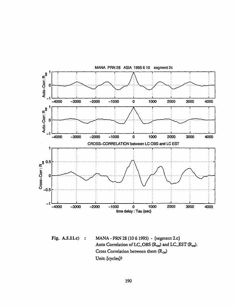
MANA PRN 28 ASIA 1995 6 10
0o
I00
-4000 -3000 -2000 -1000 0 1000 2000 3000 4000
CROSS-CORRELATION between LC OBS and LC EST
-4000 -3000 -2000 -1000 0 1000 2000 3000 4000time delay :Tau (sec)
Fig. A.5.11.c) MANA - PRN 28 (10 6 1995) - [segment 2.c]Auto Correlation of LC.OBS (Ro) and LCEST (Re).
Cross Correlation between them (R,)
Unit: [cycles] 2
190
segment 2c
-4000 -3000 -2000 -1000 0 1000 2000 3000 4000
. . . ...
..........
0C.,
U,U)0C-
a
roI
-e

0 0
0 C
o
o
o oC
)0
00 0o
(0I spue () S
T-
Lo
0;
o Io
DC
u)W
It) ,,Q
o -0c-
U)8m
E
-w0zwco0)
o 0
0
Co)
0 C
0C
) C
) N
o oQ
o
o o
o~ c
(IWs joW
o 3flnid'Y
VN
CD
C
D
v N
-ci uo
Cd
dd d
1Sa 371/ So0 31
* ".,0,o,
.0. .....
........
....... .................
..
...
...
..
...
..
....,....,...............
~........
......·
...........
..oo°
% ......
°°..°o.,°°..
* ..
.....
4
,
, : ,.
-,
,
,
, ,
:::::j~~~i?~~~~:::::::::::::::::::::.....
.o oo
o.. o,... .....
•. ,
,
.
........ :.........:.........•
..............
•.........: ........ .......
,iiiiiiiiiiii
i........................
........
... .. .. .. ..
I1r
)o-
0
-e4)
I4v
0L
I~c
£c
-)oE!
UC,/)
ý41iiU
i
.............
..............
...... ......
...... .
...... ....
............ ......
......:......
..
...
...... .
.... ......
..............
......
....
.....
..
.. ··
·~··. ....... ....l·
...·......
·...... *. ..'.*
~..............
......··•r··~
····· ,
• °~
·.·
··
5
··
'· ·
" I
! |·1
·~·
I1 ?
!o,-,
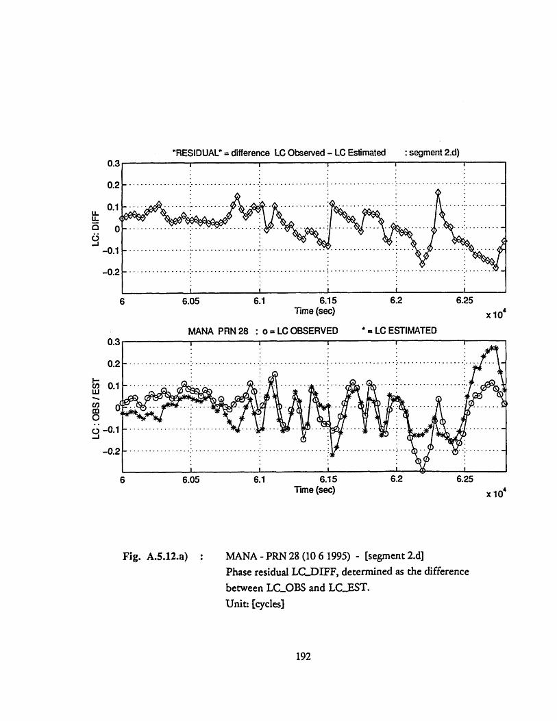
"RESIDUAL" = difference LC Observed - LC Estimated
6 6.05 6.1 6.15 6.2 6.25Time (sec) x 10'
MANA PRN 28 : o = LC OBSERVED *= LC ESTIMATED
6 6.05 6.1 6.15 6.2 6.25Time (sec) x 104
Fig. A.5.12.a) MANA - PRN 28 (10 6 1995) - [segment 2.d]
Phase residual LC.DIFF, determined as the difference
between LCOBS and LCEST.
Unit: [cycles]
192
: segment 2.d)
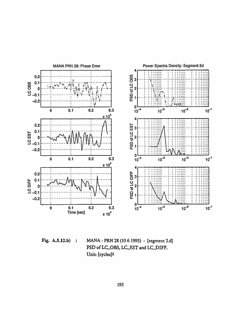
.............
.................
......•.... ......
.....
..........
..
..... .. .....
.. ...
.... ....
....
..
..
.... .•
........... ..
....
..
.........-..
r
.,
S80 0110o O
Sd
i·4.s
~··~~r...~.~...........,
L'
;f
,·r=
, =
~·
If~T.
··
·~
··;.~········.
·.
i
i'I
;r
'Y:''':''':''''
.··
.....
I I
sG
~o
l0
I
....
...... ....
70
IS3 0110o
Sd
I I
1S3 01
c0
IV
C
l cm
,-
O
1=I 01o0 o O
Sd
I I
=110 01
c'JV
C6~
C6
co
,
.....
o...'
.... ,.. ,
.. .•...... ....... .....
.o.
..... ..
.,...............,
,::::.:::::::::::.
.S,..Io,°,..'.o0
.····~·····
I'.,
CV
)
2·········
r·········
··
··
·

MANA PRN 28 ASIA 1995 6 10 segment 2d
1000 2000
-200000
-1000 1000 2000
3000
3000
CROSS-CORRELATION between LC OBS and LC EST
-1000 1000 2000 3000time delay :Tau (sec)
-1000
Fig. A.5.12.c) MANA - PRN 28 (10 6 1995) - [segment 2.d]Auto Correlation of LCOBS (Ro) and LCQEST (Rd).Cross Correlation between them (Roe)
Unit: [cycles] 2
194
U,ml0O
0
I- -10-30wCO
00
304
I I .. I .. . . . . . . . . .. . . .... ! i ....
g I I i !
00 -2000
... ... .. .. . . . . . . .. . . .
1
0.5
-0.5
-1-3000
. .. ..... ........ " ...... . ..... ... . .. .............. ............ .... ..........
. ............... ° ........° ...... ........ ...°....... ,° ° ° °... . . . ...°°°o...... .... . .. . . . .. o':-:
° I• I I
, ; i
-2000
I·
1000 2000
t
-

0 0
0It)
0 a)
(i)"S
pue (WO
S
CV
) C
i -
00
0
0r-
cNI
IJS3 01 / S
0 0-1
...
:. .
..
..
..
..... ...
.. .......
, .... .. .
..
.... ........
,......o.........°......... .......
....:.........
:........
=H
..
°..... .... ........... ., ..
..
...
,................
,
,
,.
.o
.......,....,..................o.
...
... ..
..
...
.. ..
..
..
T-
cx W
C4
C,)
' .E.
L
o -rw0wcc-w00
0le
° 0o
0
C.L
'di
C)
0 C)
C)
OY
PS1 3(O
flhldV4JV
R-
co co
C
oo~uoJeqo
GoU
g0eti0c
... ........
..
.........
...
,.. ...
.,.
..·.·.....s......
..... .........
........ .
........
... ...........
,. ..........
o......
...
.. ... .. %.
..
..
..
..
.............. ...................c....... ........
......... ............:.......
....~....... ......
(........
... .. .. ..
..
..
..
..
...'.....=
.......4..
IT0ao..
%.4o0
vC0
o'4.
I0
-, UV
0 004
V4 I-b
CO
C-)
Cd
)
0C-)
uu,
11
...... ......
......
........,...
*** ***
***
***
***
***
***
***
IC0
•
I i
I
•
II
I
=
I
I
I
.
or.-
€E
.......: ...... .......
.. ....
...... .........
.
...... ? .......
<...
......
....
n; ..
......~·
........V.....
......:.......
"S
IL
o T
.

GPS DATA: receiver: LIGO
station: 0028 satellite: PRN 09
7.5 7.55Time (sec)
90 9012 -60
0021 :. .... 5.* 30
240 300270
18 ********;*******, ,*******I*******24~0 300
270 acquisition date: 25 9 1996
station: 0028 satellite: PRN 094t6
o 44
42
40
38
7.6x l 4
7.45 7.5Time (sec)
7.55
Satellite visibility chart for PRN 09 (skymap).Elevation and azimuth of PRN 09 with respectto the station 0028
196
I
z 18
> 16W
IA
7.45
Fig. A.6.1 :
7.6
x IU
I
.......... ........ ...................................- ....... .................... - - - - - -. ... ... ... ... . . . .. . .
.* -...... ... .... ........ ...........
. ...
mA
f'
• A

LIGO 0028 PRN 09 25 9 1996
7.5 .527.5
7.5 7.52 7.54Time (sec)
Signal to Noise Ratio for L1 and L2
7.52 7.54
Time (sec)
Station: 0028- Satellite: PRN 09Data acquisition date 25 9 1996Signal-to-Noise-Ratio (SNR) for LI and L2.
197
46 7.48
(,
618IC= 16
S147.
14
12
10
87.4
7.56 7.58x 10'
16 7.48 7.56 7.58
Fig. A.6.2 :
x 10
58
= = i I I
........ ....... ....... .... ... ........ .... ..
............................... ............................................... .. .........
.............................. ..............··. ·· ·· ·· ·· ·· r · ·· · · · ·I· · · ·.... : ................ . .... .... .............·V4 ~·/·· · · ·· ·· r · ·· ·· ·· ··
I

90 9012 * 60
15 '. ... 4..5.- 1 30
18 .. ...e ... . *: , .... ... .18 ********:******* 0)************** 0O
21* **** *30
240 * 300270
GPS DATA: receiver: LIGO acquisition date: 25 9 1996
station: 0036 satellite: PRN 09 station: 0036 satellite: PRN 09
7.4 7.45 7.5Time (sec)
50
45
40
7.357.55 7.6
x1047.4 7.45 7.5 7.55 7.6
Time (sec) x104
Satellite visibility chart for PRN 09 (skymap).Elevation and azimuth of PRN 09with respect tothe station 0036
198
0)
1 20z0 18
116w
A
7.35
.. ...... ................... ..
............ .. -................. ...............
Fig. A.6.3 :
ml n I I I
I.-
·--
53~
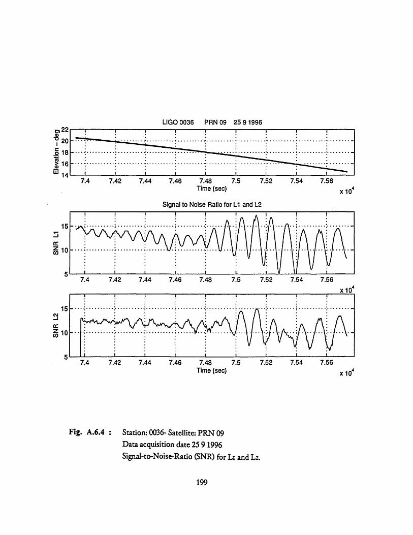
LIGO 0036 PRN 09 25 9 1996I I I I I I I i I
7.4 7.42 7.44 7.46.7.487.5.7
7.4 7.42 7.44 7.46 7.48 7.5 7.52 7.54 7.56Time (sec)
Signal to Noise Ratio for L1 and L2
7.4 7.42 7.44 7.46 7.48 7.5 7.52 7.54 7.56
................... . . .
S........... ...............
IL I i I I I I I1 I
7.4 7.42 7.44 7.46 7.48Time (sec)
7.5 7.52 7.54
Fig. A.6.4 : Station: 0036- Satellite: PRN 09Data acquisition date 25 9 1996Signal-to-Noise-Ratio (SNR) for LI and L2.
199
o22
o 20
C
> 16W 14
I I I I .
I I I I !
x 104
x 104
7.56
x 104
oo
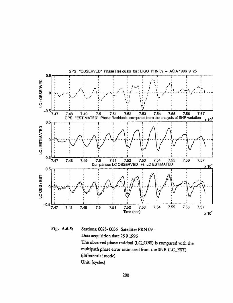
GPS "OBSERVED" Phase Residuals for: LIGO PRN 09 - ASIA 1996 9 25
5 I7.47 7.48 7.49 7.5 7.51 7.52 7.53 7.54 7.55 7.56 7.57
GPS "ESTIMATED" Phase Residuals computed from the analysis of SNR variation x 105 A.•
7.48 7.49 7.5 7.51 7.52 7.53 7.54 7.55 7.56 7.57.I i i ii i i ii i J
7.47 7.48 7.49 7.5 7.51 7.52 7.53 7.54 7.55 7.56 7.57Time (sec) x 10
Fig. A.6.5: Stations: 0028- 0036 Satellite: PRN 09 -Data acquisition date 25 9 1996The observed phase residual (LC.OBS) is compared with themultipath phase error estimated from the SNR (LCJEST)(differential mode)Unit: [cycles]
200
I I i | I jI I
I~.~ I :· I..
-0.
0.
_n
0.
?SHI! I
% A % ...... . ." " " ".'°.-.7 .... ..
-..•-..:•'•
7.47

0036 - 0028 PRN 09 - LIGO 1995 9 25
7.47 7.48 7.49 7.5 7.51 7.52 7.53 7.54 7.55 7.56 7.57Time (sec) x 104
o /5 I I I IA.": .".. ..... ... . . ".. ......;' ....
%II :. :•I. i i I
7.47 7.48 7.49 7.5 7.51 7.52 7.53 7.54 7.55 7.56 7.57Time (sec)
0028- 0036 Satellite: PRN 09Data acquisition date 25 9 1996LC.OBS and LC.EST compared for t=7.47 -7.58 10 4 secUnit: [cycles).
201
0
5-0
0.
-0.
Fig. A.6.6 :
x 104
-0._v
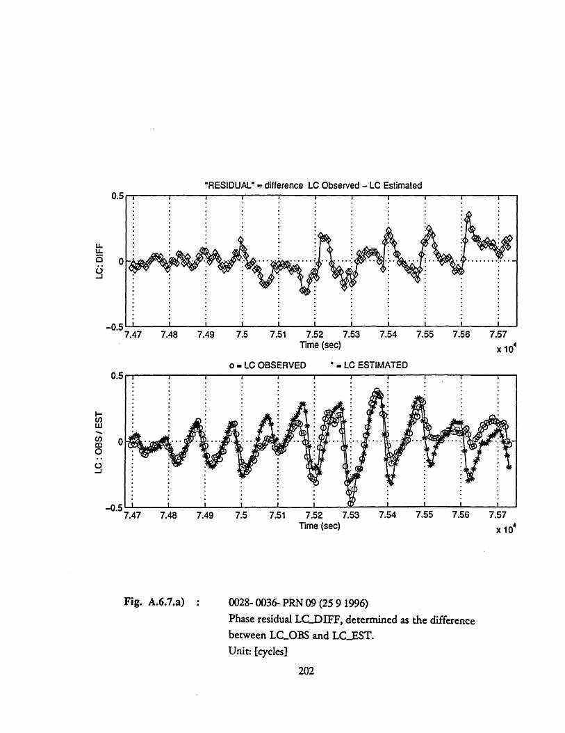
"RESIDUAL" = difference LC Observed - LC Estimated
7.48 7.49 7.5 7.51 7.52 7.53 7.54 7.55 7.56 7.57Time (sec) x 10
o - LC OBSERVED * = LC ESTIMATED
7.48 7.49 7.5 7.51 7.52 7.53 7.54 7.55 7.56 7.57Time (sec) x 10
Fig. A.6.7.a) 0028- 0036- PRN 09 (25 9 1996)Phase residual LC.DIFF, determined as the differencebetween LCOBS and LC.EST.Unit: (cycles]
202
- .•
7.47I I I I I
7.47
I · · · L · _ _ _ · ·05 EL
_-A0

LC D
IFF
I o o
PSD
of L
C DI
FF-o
o
o o
o
LC E
STI o
osi
n o
in
LC O
BSo
oNi
o
i
0)
-4 01
PSD
of L
C ES
T-'0
o
o o
o
....
....
. ..
....
...
... .
. ........
-I •
- •.
.•
••..
.. ... .
....
....
.
Aft
PSD
of L
C O
BS
-L
r C
J .ia
0L
0
0
0
.. %
.....
....
. ...
.
....
... ......
......
...
....
.....
....
. ...
..* .···r··
······.·····
·.··
··
····(
··.··
·
-L,
...
.....
.. ..
......
.....
....
• --
,.-
..-
..-.
. ...
,-
......'
....,. Io ...
....
............
.................
°.
.,
. .......
% ... o
o
....
I..
..
.. ..·
.,
.'
o
.
.. •
.. .
.. .i
. .
.···
··:!
···
i
.. ...
.
0) U'
r? I-r o c. t3
-
....
... ....
...
)·..........
.. .... ..
..
··
-L."
.
....
%
.. ..
...
....
. .
... ..
.." ...
. ...
.
....
.
......
...
..
...
...
..
...
.. .
.t.
....
• ..
... .
.. ..
•. .
.
.................
8.
.
.. ..
...
... .
... ..
.....................
....
t ..
...
:" ...
. t
....
e.°
C)

LIGO PRN 09 269 96 segment 1
-8000 -6000 -4000 -2000 0 2000 4000 6000
CROSS-CORRELATION between LC OBS and LC EST
-- 9
-8000 -6000 -4000 -2000 0 2000 4000 6000time delay : Tau (sec)
Fig. A.6.7.c) 0028- 0036- PRN 09 (25 9 1996)Auto Correlation of LCOBS (Ro) and LC.EST a(R).Cross Correlation between them (Ro)Unit: [cycles]2
204
o)0
-J0
u)ILl0wo-.JoooI-0
3
I-
U,Cd,
0
8000
8000
I

o o
o o
(i)Os pue (I)OOS
0
S3 0"1 /SB
O
"
*. .. ...... .. ...
.. ... .
... .
...
....
., oo.oo....
..............
...
.
...
........
......o.........
.....
..
o.... ....
.
....
.. .
..
.....
... ....
..... .
...
...,. ..
...... ..... ..
.....
... ..
.. ......
...."......
...... .....
..
..........
.:
... .
..
.......
.: ....
...
...... ..... .
...... .......
.... .
a.
·I
!· i.
Co
0 0
0U
) 0
U)
0 U
)C
m
CsoN
V-
I-
(o o
i o
ro
lolli
Go
,0 0:
U)
C0)
a,.C
Lt3OO0.C
)
CCUC
......:.......
...
..
.... .
: ......
:::::::::::::·::::::::::::.::::::......-... .
..
o...
.o..... ..
.....
..... .
...... .
...... .
...... ......
........ ......
...... .
......
:::::::::::~:::::::::::::::
.. ..
...
.. ..
.. .
.. .
... ... .... ..........
........ .
..
... ..... .... .
%.. .
..o.
o. ... ..
.o
... ...
... .. ....
.... .
..
.......
.... ..
·-·-
·--:··*****·
-- --
··
·*
·**
*
******.****** ···*** **r
*** *.* ***
U)
0)0a."CC
cLU?
CO)cl)o r)0ccOC
'I
.....
o..
.
.. .S
.............. .....
....
•
..
••
-• •• •
iiiiiiiiiiiii
%4-0
00r'.o0C,)
0
......
.......
.. ..
..... .
.
..........
...... ........
..................
::::::::::::::::::: ** ::::::::::::
............ ...
..
....
......
. .· ·.
.··
...
......
*******
****:*
***oo:-*
**,*
*.*
*****
...... .......
....... .
.*.... ..*
.*.*
.*
.
r····.. ... ..
..··~
······
... .. .
... •........
...... :.......
....
.. ....
..:
......
I I .
I.....
...
.......
......
..
....
...
...
......
.....
.....
N'4-arm
I
i i
t A
-
•
II
II
•
4 ,-
> VCCa
ITCo
(o> r

90 9012- 60
15 0 .... 43
18 ....... ...... :0 ....... 0*Z.
21 . 30
240 ' 300270
GPS DATA: site: LIGO acquisition date: 26 9 1996
receiver : 0028 satellite: PRN 15 receiver: 0028 satellite: PRN 15
CD"O
I 310
I-3052 305
300A
Time (sec) x 1047.4 7.5 7.6 7.7 7.8 7.9
Time (sec) xlO1
Satellite visibility chart for PRN 15 (skymap).Elevation and azimuth of PRN 15 with respect tothe station 0028
206
Fig. A.7.1 :
wAhi •

LIGO 0028 PRN 15 26 91996
.. ... .... ... .... ..... ...... .. ... ...... ....
7.5 7.55 7.6 7.65 7.7 7.75 7.8 7.85x 10I
Signal to Noise Ratio for L1 and L2
in7.8 7.857.6 7.657.5 7.557.45 7.7 7.75
7.5 7.55 7.6 7.65Time (sec)
7.7 7.75 7.8 7.85
x 10'
Station: 0028- Satellite: PRN 15Data acquisition date 25 9 1996Signal-to-Noise-Ratio (SNR) for Li and L2.
207
50so40
0.1> 300Mw
9207.45
20
.1n
7.45
I I~ I I I I I
....................................................
I I I t ____ VI
Fig. A.7.2 :
I
.. .... ..... .... ...
-
_4
I-
I

90 9012 - 60
15 .... 45.- 30
18 .......... . .. ,* * * I * * * 0r. * . '. . '
21. . '* 30
240 300270
GPSDATA: site: LIGO acquisition date: 26 9 1996
receiver: 0036 satellite: PRN 15315
a0
1 310
2 305
Q0nn
7.4 7.6 7.8 8Time (sec)
receiver : 0036
7.2
x 104
satellite: PRN 15
7.4 7.6 7.8 8Time (sec) x 104
Satellite visibility chart for PRN 15 (skymap).Elevation and azimuth of PRN 15 with respect tothe station 0036
208
40
30
20
in7.2
Fig. A.7.3 :
r .. .. ..7 .........********************f - ****** **********
· '
· '
I
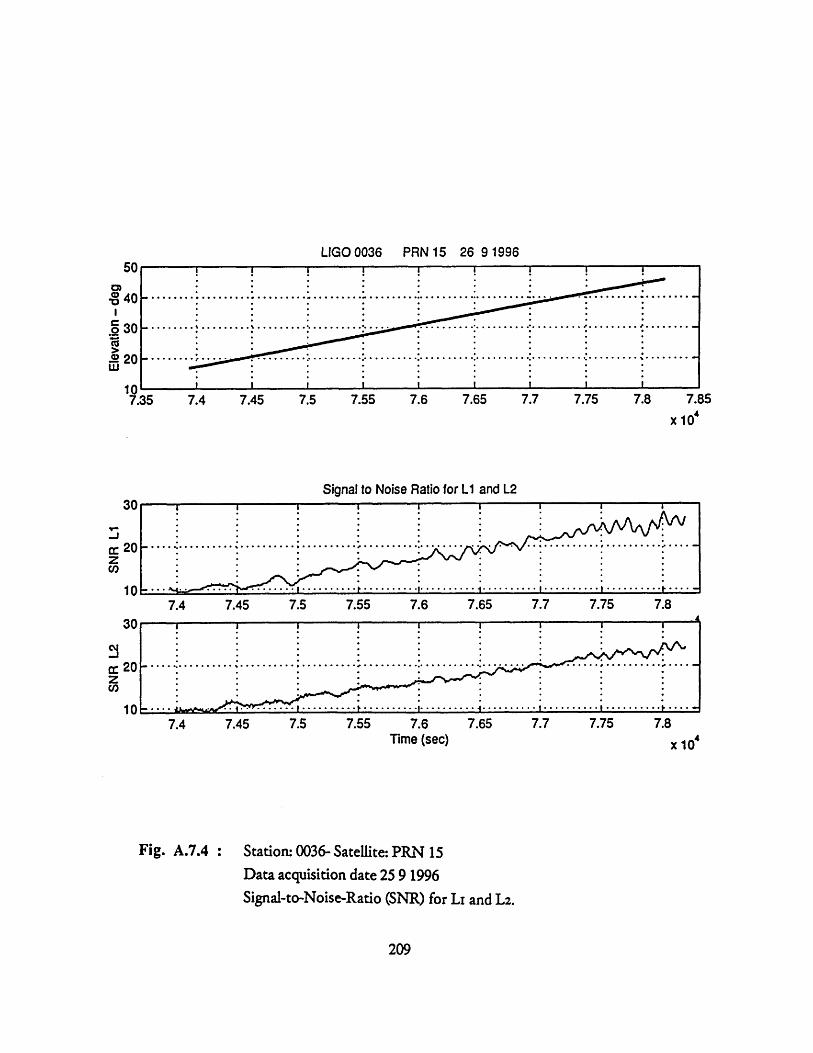
LIGO 0036 PRN 15 26 9 1996
7.4 7.45 7.5 7.55 7.6 7.65 7.7 7.75 7.8 7.85x 10
Signal to Noise Ratio for L1 and L2
20
7.4 7.45
20
7.4 7.45
7.5 7.55
7.5 7.55
7.6 7.65
7.6 7.65Time (sec)
7.7 7.75
7.7 7.75
x 10
Station: 0036- Satellite: PRN 15Data acquisition date 25 9 1996Signal-to-Noise-Ratio (SNR) for LI and L2.
209
I I I I I I I I 1
46............. .. ... .......... ...... ·.. ....... .........30 ..... r......... r..........s....'..~....~...........s...20 ... ... ...~~.·.. ... ....... e*...... ......................''' ''' s··....
7.35
. . . . . . . . . . . . . . . .. ......
- I l* *............ I .....-
..• .•.............. . ;.. . .. ....
. .... .... .... .... .... . ... .... ....
Fig. A.7.4 :
--I
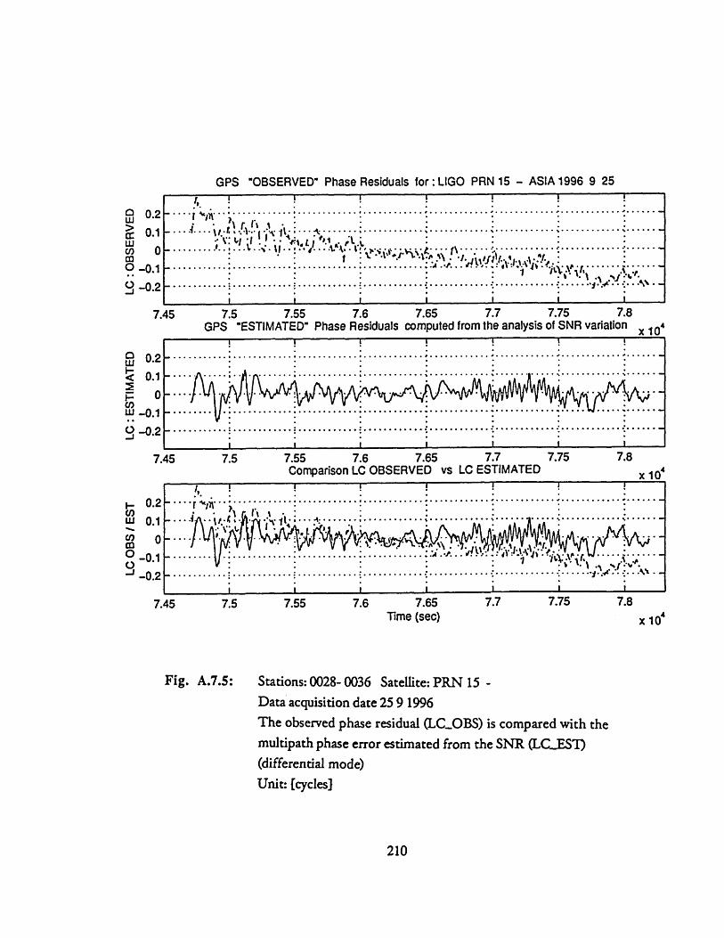
GPS "OBSERVED" Phase Residuals for: LIGO PRN 15 - ASIA 1996 9 25
... ...... ............... .... ............ ......--------- ·C-- ------ ----- -------- -- -- -s··
I I I , I 1 I
7.45 7.5 7.55 7.6 7.65 7.7 7.75 7.8GPS "ESTIMATED" Phase Residuals computed from the analysis of SNR variation x 104
7.5
7.5
7.55 7.6 7.65 7.7Comparison LC OBSERVED vs LC ESTIMATED
7.55 7.65Time (sec)
7.75
7.75
7.8x 10
7.8
x 10
Fig. A.7.5: Stations: 0028- 0036 Satellite: PRN 15 -Data acquisition date 25 9 1996The observed phase residual (LC.OBS) is compared with themultipath phase error estimated from the SNR (LC..EST)(differential mode)Unit: [cycles]
210
0 0.2uJ
ccrr" 0.1uJwC, 00 -0.1, -0.2
S0.2
0.1~ 0
S-0.1
U -0.2
*.***---- ****.* . * . ... **
..... . ............ ......... . . .. ...... . . . .......... . ........... .... ..... . ..... ... ...... • ......... • ......... • .........
7.45
0.20.1
0-0.1-0.2
7.45
.....r . .... .' .............................. : ...... ......I_ _
I I I i I I

0036 - 0028 PRN 15 - LIGO 1995 9 25
7.5 7.55 7.6 7.65 7.7 7.75 7.8Time (sec) x 10
7.55 7.6 7.65Time (sec)
7.7 7.75 7.8x 10'
Fig. A.7.6 : 0028- 0036 Satellite: PRN 15Data acquisition date 25 9 1996LC..OBS and LCEST compared for t=7.45 - 7.85 10 4 seUnit: [cycles]
211
U.3
0.2
0.1
0
-0.1
-0.2
7.45
0.3
0.20W 0.1UjmCO 00
-0.1-0.2
-0.2
7.45
S• I I I -' •........l.....A......................... . .. . . . . . . . . . . . . . .
. ........... .............. .. ............ : •• ...... .......
......... . ........................... ....... .•."* " -" _'u : r!j,,:, IP•...,.-
^^
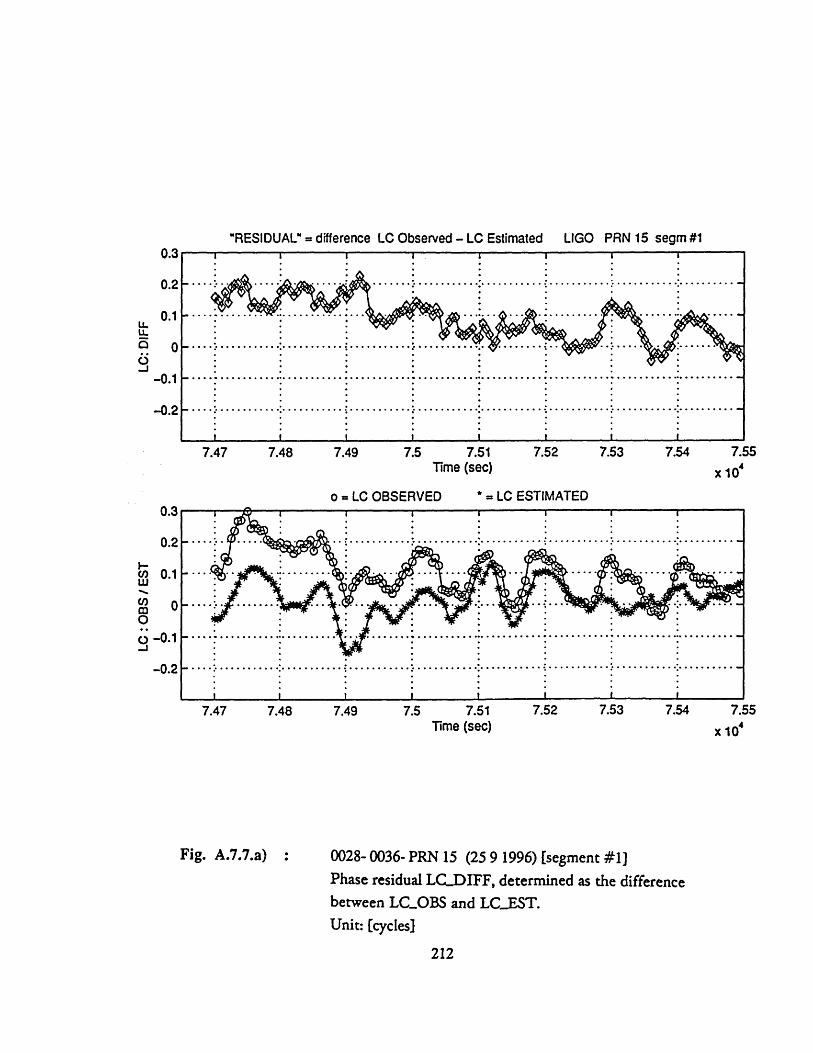
"RESIDUAL" = difference LC Observed - LC Estimated LIGO PRN 15 segm #1
7.47 7.48 7.49 7.5 7.51 7.52 7.53 7.54Time (sec)
o = LC OBSERVED * = LC ESTIMATED
7.47 7.48 7.49 7.5 7.51 7.52 7.53 7.54Time (sec)
Fig. A.7.7.a) : 0028- 0036- PRN 15 (25 9 1996) [segment #1]Phase residual LCDIFF, determined as the differencebetween LCOBS and LC.EST.Unit: [cycles]
212
7.55x 10
7.55x 10

-*****
*..
o .
...
..
..o
:: ::::::::::::::::: :
..-.
....
..
........
..
..... .......
......
..,
...
..
...o.
.....
..
, .
.., ..... .
' .
.S.
...........
:
.,
..
• ..r...r. ........
'.;-
...:............. :>:.
;. .' .-..... :....
..\.r.~
,.r... "·
··
··
,· ·
·s
° ,,••,·
°o°°oo
•
··
··
·. •r
S) "
C0
C
~1
-0
S8
0" 31
o C]Sd
.... "•;"-•.
...
...
..'
• ..
*.
.... ·
.-.
'-.:
:... ...:..
• .. .,
..
.., .. ....:. .
:'>
," ,,,,,,
··
·:·
··
-i:
-:...
.•
•
,
0M
Cr-
-i
SGO
30
I
0^
I) 0 C')
CJ
1 0
IS3 31 lo 0S
d
...
.. ..... ....
.. ......
.... .
... ....
...
-
..
,.
.o.
.. ,,ooo..
.. ... .... .. .'.
o. ..
o,,
,***e
*oo.*oo°
o *oo *oo
i ll#
.,,•,.,.,.,.,•
.• •
o
°·.
Lqr
M~
c 0N
--
1I-1 3 1
o Q
Sd
wEC
, -
IS3 0
1-I.I
0"
1g~
.... ... -..... :.... .
•..........
.: ..... ....
...
:..... ......
S: i
: :::
...:
-. .
.....
.. .A
-····
·
tp 94. 4u,0 P,4J~
L4
U04O
'0-00
M•
C,..oo• ,,
Q',I
"
f
,,

LIGO PRN 15 26 9 96 segment 1
-4000 -3000 -2000 -1000 0 1000 2000 3000 4000
-4000 -3000 -2000 -1000 0 1000 2000 3000 4000
CROSS-CORRELATION between LC OBS and LC EST
S. . .......................... ..... ............ .. ......... .......... ........................... .
S- 0 .5 ............................. ............................ v ......................................
-1 ,
-4000 -3000 -2000 -1000 0 1000 2000 3000 4000time delay : Tau (sec)
Fig. A.7.7.c) : 0028- 0036- PRN 15 (25 9 1996) [segment #1]Auto Correlation of LC..OBS (Ro) and LCEST (R).Cross Correlation between them (R)o
Unit: [cycles] 2
214
CC8
0 0I
o<3
rr
0 00
<1
0o0 0
02
I I.. . . .I I I I .I
•
.I I I II I7
.I ..... .. .. .... .......
..................

Cohe
renc
eS0
0o
0
io
:.
b bo
AM
PLIT
UD
E of
SO
(f)0
0 0
0
00
C0
C)
0 0
CD
()
a
Cr
o
.,
0 O 0 C, *1 U) 0 0. 0
LC O
BS
/ LC
EST
S000
S o
.io
c
SOO(
f) an
d S
(f)
r b0
D
00
0
o0
0 0
0 0
aC
I.
0 o= m 0 CO
oC
)/C
>,>
0
'1-9 cD:1
=
0 C)
CD
(D=3
40
-'
C
C)
to
... .
....-
. .,-
..-.
..-
.--
-
....... .
.. ..
.
o,"·.
··
·~1
''*''t=''''
S'
' ,+.,' '''"
......
......
......
......
......
....
o...
.o.. O.. o
...
.........
..
...
...... ......
......
...... .. ..
~~~~
~' ~
~ ~ ....
~...
....
....
....
..... ... .
..
..
... ... .....
.............
......
.........·
·'
......
......
......
......
..·····
......
......
......
......
......
..~~
............
....
.. .
............
.. .................
....
....
....
.
... ... .
.. ..
...................
> .....
.......
~~
............
..................... .
......
. ...
..··~···,......
............
··
......
.....
·~ · · ~·.
....
....
....
. %
......
·····
····. ...
. ....
.·
--
......
.*..
....*.
......
..*...
...• ,...
.. .......
.............
.+
.;
3 i~
i i
.....
....
...
..
........o
...:
::::
::
::*::
:::
..........
.. ......
. ......
*......
*...................
......
*.......
...... .. .
.... .
.... .
.............
··
·
.................
VL O v
%a
ft.
)o
) .
11
~ m

"RESIDUAL" = difference LC Observed - LC Estimated LIGO PRN 15 segm #2
..........
...........
-.....-- -.
I I I I I I
7.58 7.597.57
o = LC OBSERVI
7.57
7.58 7.59Time (sec)
ED *= LC ESTIMATED
7.58Time (sec)
7.59
7.6 7.61x 10,
7.61
x 10
Fig. A.7.8.a) : 0028- 0036- PRN 15 (25 9 1996) [segment #2]Phase residual LC.DIFF, determined as the differencebetween LC.OBS and LCJEST.Unit: [cycles].
216
0.3
0.2
0.1
0
-0.1
-0.2
7.55 7.56
0.3
0.2
0.1
0
-0.1
-0.2
- ·-- ·----------- I--------- - ------- ***---- --- -
.-............ ............... :....... ......
I I I I I I7.55 7.56
--

• ..- .
........*
... ....
S....
..... -.
..... ......
..... .....o
...
..
..
• ..... .. .
..
...
..
.....
....... .....
.........• °.
..
·.
• '° ° •°°
.-.°.
.•. ..
•
..c··r~
~~
~~
·•
• .··
•·.·5
·
·s
··
··
·
CD *~
J C 5U
0r
o
6
6o80
"1ijo GSd
2:
o.
.. .
/
...
...
..
I.5
',.
.BO
.
SB
O 01I
..
...
....·
..
o.
...
.::'::::::':
:: •:
::.
..........
.. ......
.... ....
..
S.........
...... .....
..........
....
.....
:.
.-. ..:----.
..' ...
.'. ...
S.
' "
''•...............
c..
:N
...... .....
,....•
::.,::: ..
""" :; I"
0
So
Io
o
IS3
0" 1o G
Sd
18
01Isa O
C
........
•...........
.: ... .. .
... ...
... ...
..
.
.-. ..--.--.- .--..-.
..
.................
•...
•.: ..... .
.........
.. ...
..... ..
.....
I
CD
C
o C
o
zw00 oJo
aS
d
cotDE~"-.U
)-l=
CD
u)
==110 0"1
~4QO
NV
-
u0 P,1 10
ul
8e P4:
T-
t

LIGO PRN 15 26 9 96 segment 2
-3000 -2000 -1000 0 1000 2000 3000
-3000 -2000 -1000 0 1000 2000 3000
CROSS-CORRELATION between LC OBS and LC EST
-3000 -2000 -1000 0 1000 2000 3000time delay :Tau (sec)
Fig. A.7.8.c) : 0028- 0036- PRN 15 (25 9 1996) [segment #2]Auto Correlation of LC.OBS (Roo) and LC.EST (RE).Cross Correlation between them (Ro)Unit: [cycles] 2
218
Io4
o
0I
OT
a: 0.5
0
o 0
-0.5
-1

U)
aQ)
00-
0~a.
C',0
cC(A :::::::::::::::::::::::::::::::::::
.....
* ..... .................
°.....
.....:.....:.....:.....:.....:.....
.. ..... .
-...... .
...
...
.........
..
............
o··. ··
r·· 0
0
So
0
0
()S PU
(i) s
C')
CJ
,
0
0
0
I03-
o O
01r
0 0
0 0
0 0
Co )
o
,•
C') tJ
--
V(l)
S
oIC
lnIld
4'JV
C)
x I
copO0
tor0cu
U)EE
u-OO0zwCo
ccU
) W00
o r,-
coc0
cj
1S3 31 / SBO 0
1
o o
I o
........
..... .
.. ...... .....
..... :.....
.. .
.. .
.. .:.
..
.......
..
.........
..........
.... :.....
• ..... :.....
• ..... :......
3
.8.··
··
·:
··
i ·
··
··
.8···
··
( ·
·.·
·(
··.
8
.·.
3
.8.···
··
··
··
·
:::::::::::::::::::::::::::::::::::
°.°.°°°..°•.°.°°°°. .. °...°
...
.. ..
.............
..... .. ....:
.·o..'..,..,,o'o,,.,.O.,.,°,,,
°....°.°.°.°l.....°oo..°°°oo.o..°
I_0,-
·- ·
··
··
··
··
···
7
···
0C>
IvC)0
ISr-
:: ::
.:
: .:
: ::
: .... .- .
..
::::.* .:::: l:*:::::i::::. :: M::::......*.......*.... .. .................
...... ......:........
.....
... ..
.......
.. ..
.. .
....
**.
***o*....
*.....°..
.....
..o.
........... ....
.,. o.,0,,
•o.,..,•,,..,,.,,
o
D
o%
4.4
0
2) I
0%8
-a0
0C
f)t/
ob
oo o
8
iouat-
···
.m

"RESIDUAL" = difference LC Observed - LC Estimated LIGO PRN 15 segm #3
7.63 7.64 7.65Time (sec)
o = LC OBSERVED * LC ESTIMATED
7.63 7.64Time (sec)
7.65
Fig. A.7.9.a) : 0028- 0036- PRN 15 (25 9 1996) [segment #3]Phase residual LC.DIFF, determined as the differencebetween LCOBS and LC..EST.Unit: [cycles].
220
I I I I I II I I i I .
61
0.3
0.2
0.1
0
-0.1
-0.2
7.4
U.%3
0.2I-.)0.1
S-o.2-0.2
7.62 7.66
- --- ~ ~~~ ...-- - ..-- .- .-. . .---
I I I........... .. . . . . . .. . . . . . . . . . . . . . . . . . . .. . .
7.67
7.6731
68
68
7.
x 10
7.
x 107.62 7.66
I I I =I
7.
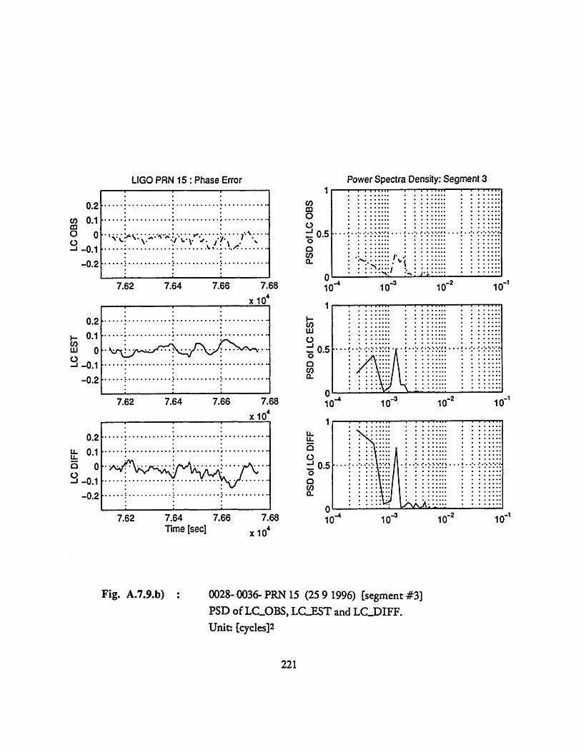
..................
.
.....................
.......... %.......°
.... ..... ....
o..
...................
4
..........o
..........
o,ro1r
0o C
SS130 0110 GSd
*
I;
I
Sg1
31
T
%
coIn'1
0C
o
T-
co
tDr,,,
o- o
LA
o
S
193 0110O
GS
d
o..'.°o.°.o..
..
..
.....
.....°
°°
°. ..
°.
........
......
,-°°
.........
•.. °
.... ....
.°..................
..°....%...°*..°.....
..........*.........
.........
°............°.........iii
ii
ii I·
Cl.
ECOQ)
Cu
o0.C
,)
co<.:
CD
F..
I I
'i
-110 01 Jo GSd
I I
-_-1110 01
It
..
..,
,
,
,
..
..
.....
.........
..........•..........
.........
....
°...
°..°°.°.°°,.....°.
°.°..,,.°.....
- .. ;*. o .. . . ..
. .o
0···.· ·
····
r-"
4.
140
.4OUo
|
oe
('4 "2
r-o
co E
C?01c
'I.g
1 I
I "
i I
2...·.. J...·....
·..·r··~·~~··.~··~~ ~
··
··
··
··
··
·
-u
IS3
0
01
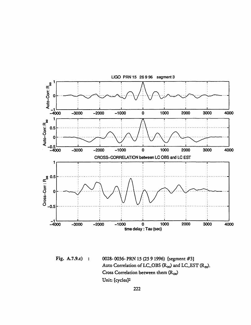
LIGO PRN 15 26 9 96 segment 3
-3000 -2000 -1000 0 1000 2000 3000
-3000 -2000 -1000 0 1000 2000 3000
CROSS-CORRELATION between LC OBS and LC EST
-3000 -2000 -1000
Fig. A.7.9.c)
time delay: Tau (sec)1000 2000 3000
0028- 0036- PRN 15 (25 9 1996) [segment #3]Auto Correlation of LCOBS (Roo) and LC_EST R).Cross Correlation between them (Roe)
Unit: [cycles] 2
222
Sa:8Eo0
I0-4000
0
oo
I0'S
-4000
4000
4000
0.5
0o-u,
U,
.. . . . . .. . . . .
. ............
-0.5
-1-400 4000
-1d
........... .. .....:
........... .... ''
. .
S- -··
30
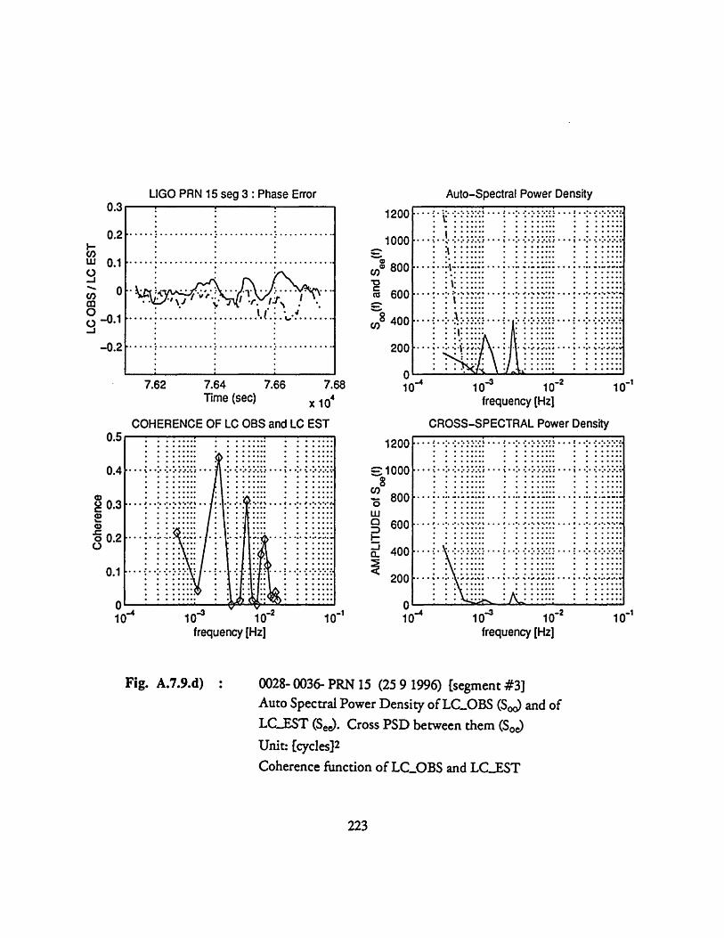
0
0 00 0
)
coo
C
*OC
()s pueo
oo AcO
*:..........
1.... ......
:~::::::::::::;:::ii: :::::::::::·:::::
.. .... ...• ...
...
...
...
....
... ...
....
S.:......:.....
•.....{......:......}.....
°:~~
~
~~ ..
..
..
...
.... ......
%
..
, ....*... ...... ...... .
...
.:
...
.........•
i i
: .i
.ii i
i i
iii iiii
2Co
Coc,
U)x
coE
clJC
R1l_
* t.:°°°
.o
·o..
.·.· -.. ...
....
°-°.o
o:
.oo ..... ......•.. ...
..> .! .
.. .. ..
...... ... .. ....
..
.....
...... .... ............
....
..
.......
•.
··~''('
·•
•
•··
··
..........
....
......
°°°....°°°°o~~~r °.o°
°°°°°
,°o
°°°,° ° o• .o.,.
o. ° •° °.*.o.O'..
• °
o
S..
... ...
.... ..... ....
...o.
..
..
..
.1"'
"' ·~.··
.1-o
o
o
o
o
o
CC
0j
0 0
0 0
0
(I)CeS
0 0 :n LldINV
C
o o;
o C
0 0
0
0
0o
CM
1I
>
X
>
C?C
)
t:)"
0*0~
.a1
Db
C)S
IcrC
.,
Ca,
".0r*
*1_
cySo"
cr(',
a)ar-0'*
17
O0C/,)o utn
E
0
oo0Uk:8P
c U
u-ao,, .....
; .
........ ......
° ...
0 ..
:::
: :::::::::
: : :
........ : .....
.... ..... .....
: .. .
...•
.......
...........
•:•
• o,
,,. o.0
,•o
oo,
.....
... ...
::::
:::: :::
:::::::: : : :: : :
....... :...... •...... •.
...: .
..
.... .. ..
.. ......
......:.
..
.. ... ...
.....
.. ...
... .. .. ..
.. ..•
..
..
..
..
..
% .....
..
..
..
..... .....
.....
i.:*..... ...
......
IS3 o1
/ S1O0 01
or-
(O
T-I
I
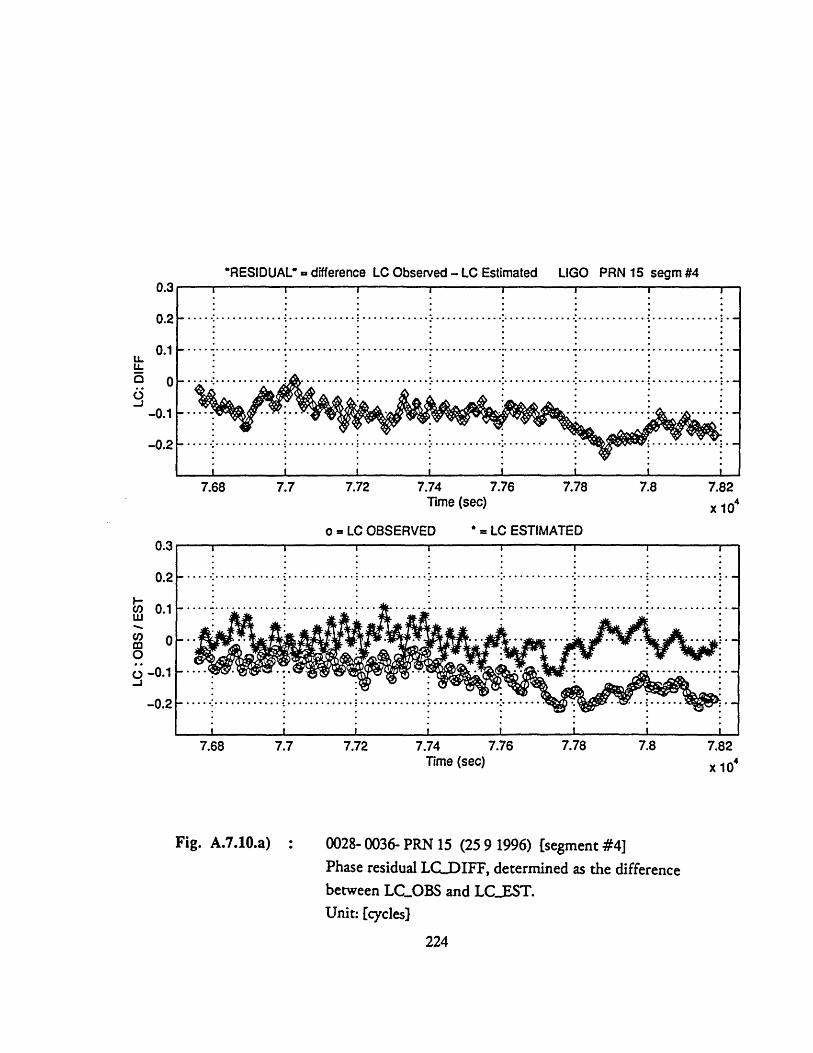
"RESIDUAL" = difference LC Observed - LC Estimated LIGO PRN 15 segm #4
............ :• . • o • ,"" ·
H II ; ;I
7.68 7.7 7.72 7.74 7.76 7.78 7.8 7.82Time (sec) x 10"
o = LC OBSERVED *= LC ESTIMATED
...........-........ .- ............... : ...............-- --- ---- ............. ...........
*17.68 7.7 7.72 7.74 7.76 7.78 7.8
Time (sec)7.82x 10
Fig. A.7.10.a) : 0028- 0036- PRN 15 (25 9 1996) [segment #4]Phase residual LC.DIFF, determined as the differencebetween LC.OBS and LCEST.Unit: [cycles]
224
0.3
0.2
0.1
0
-0.1
-0.2
0.3
0.2
0.1
0
-0.1
-0.2
I i i i

...,. .... .$ .
...
..
.•.0
o.0. ..
.. ....
.....
....
o
..
0 ...., .,. ..
..............:.....
o:7o
0-
.•••.5
.-.. ••••
..o ..
° ....
..
..
, .
..
•.
..
.....
.....
......
SGO
01 J0 OSd
:::::::::::::::::::::° ·.' ..
o ;o.
.•, ,
..; ..... ;....•.•"·
··,,,·.
•
·~··1·5
·
·5·
··
··
··z "'
'
··
'" ۥI
C)
$80~ ~
' 0" o
r
*.
: ..
SBO 31
Co
Ir
..%
.................
:...........a..
....................
.. ..
.,..... .....
.. ......
.......:
..... .....
.......
.
... .... .....
:....
• ,-.....-. ..
.•. .
··"" ·
·'r
60NCY0
470
I
........ ....
....
.: .... .
.. .
.; ..
..........
....
.....
.a
.|
.I.···t··
··
.a..a.
So 1
oS
d
-10 3V
o
Sm C
IS3 oi lo aSd :jJ1(a oi lo aSd
0
'
c"I4uc 4
o 44
UM0oI~uenr
008 P41_
C,
Elw
-IQ
10 31
I'
" "'
"'"
a,·~:...·....···
: : ..
.
IS311

LIGO PRN 15 26 9 96 segment 4
-0.8 -0.6 -0.4 -0.2 0 0.2 0.4 0.6 0.8 1
CROSS-CORRELATION between LC OBS and LC EST x 104
-2000 -1000time delay :Tau (sec)
Fig. A.7.10.c) : 0028- 0036- PRN 15 (25 9 1996) [segment #4]Auto Correlation of LCOBS (Roo) and LC._EST (Ree).Cross Correlation between them (Roe)
Unit: [cycles] 2
226
..
0
o
Io1_
-1
0.5
0I..oa
t-
I I
... . . ..
-0.5
.1-4000-4000 -3000 1000 2000 3000 4000
_· · I · · · ·
I
.8
. . .. . .. . . .. .. .. . . ... . . .. . . . . . . . . . . . . . . . . . . . . . .
'''°
!

c)Ca00)oa-0.C
,
IS3 01
/ 801
0"
O() s o
OanldN
Vd
V- CO
x W
Mco
cr"oC.)
zIl0
co co
v C
0 0
0 0
OD
uOJL
IloO
.....
..........
0
°°...........
.
...
......
...................
.........
..........
.......
..
....
..
... ......
... ...
.....
..........
... ..
.....
..........
..°........
.........
.. .
......
o
... .....o .
...
..
....
..
..... ..
...
..
..
..
°.°°.....1
··..
o........
..
°
.
°,° .°o
°o•
°°°
oo°
°•°...
......
....°
.....° ......
...°
.°..........
.,...............................
.o ° .
..
.° .....
°.. .
°°
..
.
...
0
...
..........
0........
.1...........
.......... ..........
..
..
°°° ....
..
...
...
..
o 0
o 0
o U
)(I)•'s
pue (I) °°s
0Co)LO
o*'
C,
0oU-4
04,t)
Sc
o
T.
...
-....
..
......
;......
-.
-.
....
.. ....
....
... .............
............. ......
.............
....... .
...
......... :
...... ......
...
... ..
.......:...... .....
?.......;......
....... ......
... .
..
.... .......
.. .~
...~...
.. ....
...
..~~~.. ..
... .... ..... ......
....... ..... .
.... .
........
I-0wa)LC
,
a-Z cco.J.0)a)zo00.--
9-T04)0
L4
,)0 41
.o£n
B
I
o0u3
Io
C
T--
IO
r-

90 9012 - 6015 =. ....
18 ........: ....... 0 :******.*.*..*.. 0
21 : 30
240 300270
GPSDATA: site: LIGO acquisition date: 26 9 1996
satellite: PRN 25170
165
160
7.5 7.6 7.7 7.8 7.9Time (sec)
7.
receiver: 0028 satellite: PRN 25
5
x 10'
7.6 7.7 7.8 7.9Time (sec) x 10'
Satellite visibility chart for PRN 25 (skymap).Elevation and azimuth of PRN 25 with respect tothe station 0028
228
receiver: 0028
Fig. A.8.1 :
.. .. .... ......... % ................ ...... ..... .
..
.°°
-1 gzr%

LIGO 0028 PRN 55 26 9 1996
7.65 7.7 7.75
Signal to Noise Ratio for L1 and L2
7.65
7.65
7.7
7.7Time (sec)
7.75
7.75
Fig. A.8.2 : Station: 0028- Satellite: PRN 25Data acquisition date 26 9 1996Signal-to-Noise-Ratio (SNR) for LI and Lz.
229
7.6
. . I I .
35
-. 30I
. 25
g 20
7.
25
20
15
10
7.
25
20
15
10
7.5
7.85x 10
I I I I
I I I I I.oo °.. .. .... . .........o.o...o..o.......... ..... ........................ .. .. . ...
I g
7.85
7.6 7.8 7.85x 10⁴
55
55
5
5
5
II I II A A A................ ................ .......... ..... ................... ...................... ... ... ... ... ... ... ... ... ... ... ...

GPS DATA: site: LIGO
receiver: 0036 satellite:PRN 25
Time (sec) x 104
90 9012 - 60
15 45....... 30
18 ....... ; *.... ..*0*...... .......* 0
21 30
240 300270acquisition date: 26 9 1996
receiver: 0036 satellite: PRN 25
Time (sec) x 104
Satellite visibility chart for PRN 25(skymap).Elevation and azimuth of PRN 25 with respect tothe station 0036
230
Fig. A.8.3 :
9
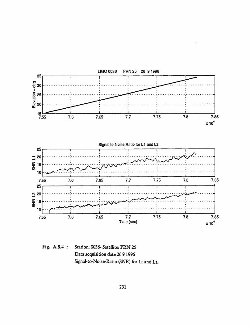
LIGO 0036 PRN 25 26 9 1996
7.65 7.7 7.75
Signal to Noise Ratio for L1 and L2
7.65
7.65
7.7
7.7Time (sec)
7.75
7.75
Fig. A.8.4 : Station: 0036- Satellite-. PRN 25Data acquisition date 26 9 1996Signal-to-Noise-Ratio (SNR) for LI and Lz.
231
35CM` 30I
. 25
& 20LU
ýj7.a
25j
7.85x 10'
zu15
10
7.5
25
20
15
o7.7.5
7.6
7.6
-I-- I·~~···~~~ I~-''''' i········--······
I II ___I
7.85
7.85x 10'
1_ • • . . .I
| | | | • i
......... ......... ......................... ........... ......... ~.....
................. ............... ...... ... .. ...... . ... ....
. . ... .. .. .. .. . .. .... . .. ... . .. ... ... ..... .....
55
5
5
.... ... ... .................. ..... ..... .... ...
.... ... ... ... .... ... ... ... ... .... ... .. ... ... .... ... ... ... ...

GPS "OBSERVED" Phase Residuals for: LIGO PRN 25 - ASIA 1996 9 25
55 7.6 7.65 7.7 7.75 7.8GPS "ESTIMATED" Phase Residuals computed from the analysis of SNR variation x 104
0.2
0.1
0
-0.1
-0.2
7.
0.2
0.1
0
-0.1
-0.2
7.
7.6 7.65 7.7Time (sec)
7.75 7.8
xlo4
Fig. A.8.5: Stations: 0028- 0036 Satellite: PRN 25-Data acquisition date 26 9 1996The observed phase residual (LC.OBS) is compared with themultipath phase error estimated from the SNR (LC..EST)(differential mode)Unit: [cycles]
232
I I I I I
S...... .................. ........ . ............. ...........................
. ... ... ... ... ...... ..... ..... • . '..... o........... ................ . o...... .... .... ..... -.......I I I I I
55 7.6 7.65 7.7 7.75 7.8Comparison LC OBSERVED vs LC ESTIMATED x104
0.2
0.1
0
-0.1
-0.2
7.5
_ I - II. ... ... ... ... ... ... ... ....· :·· · · · · · ·................. ·; .. .. .. .. .. . . . .. .. .. .. . . .. .. .
II I I I
. I . I................ ·.·! · · · · · · · ·... .. . . .. .: · · ·,·· ·.. .. .. ... ..t.... . .. .. . .... ... .. . ... .. .. .
..
....... ..... I .. .. "''
I I I I I
I I I I I
I | g I • •
..... ...... .. o... ... . ... .
I I I I I
5

0036 - 0028 PRN 25 - LIGO 1995 9 25
7.6 7.65 7.7 7.75 7.8Time (sec)
7.6 7.65 7.7 7.75 7.8Time (sec) x 104
0028- 0036 Satellite: PRN 25Data acquisition date 26 9 1996LCOBS and LC..EST compared for t=7.56 - 7.9 10 4 secUnit: icycles]
233
I I I I I 10.2
-0.1
-0.2
7.55
0.2
uI,,I
cc
Cn 00o -0.1
-0.2-0.2
x 10
7.55
Fig. A.8.6 :
1

0036 - 0028 PRN 25 - LIGO 1995 9 25
7.6 7.62
7.62
Time (sec)
Time (sec)
7.64
7.64
7.66
7.66
0028- 0036 Satellite: PRN 25Data acquisition date 26 9 1996LC_OBS and LC_EST compared for t=7.56 - 7.7 10 4 secUnit: [cycles]
234
-0.1
-0.2
[ I I I I I ~
I I I 1 II
7.687.56
-0.1
-0.2
7.56
7.58
7.58
x 10
... . . . . i
I I i
I~~~~ Ir. i \
I'r·· J .~.
." ." "........ . ........ . .. .. " .... .. "....... .... ..... .. .. .: . . . . . . . . . . . ... .: . ... . • ...... i ......... -...• -...r ... .. .....; .... ... .. ...'1:: I r. I I I . . •I - i .I - - - -- - - " I• -'.. . . .'-. . .. . . . !. . . . . . .. . . . . . .. i i . . .•- -.. .
Fig. A.8.7 :
7.68
x 10
::i

"RESIDUAL" = difference LC Observed - LC Estimated LIGO PRN 25 segm #1
7.56 7.58 7.6 7.62 7.64 7.66Time (sec)
o = LC OBSERVED * = LC ESTIMATED
7.58 7.6 7.62 7.64 7.66Time (sec)
7.68x 10
Fig. A.8.8.a) : 0028- 0036- PRN 25 (26 9 1996) [segment #1]Phase residual LC.DIFF, determined as the differencebetween LCOBS and LC..EST.Unit: [cycles).
235
0.2
S0.1
o')
0
o -0.2
-0.2
7.68x 10
7.56
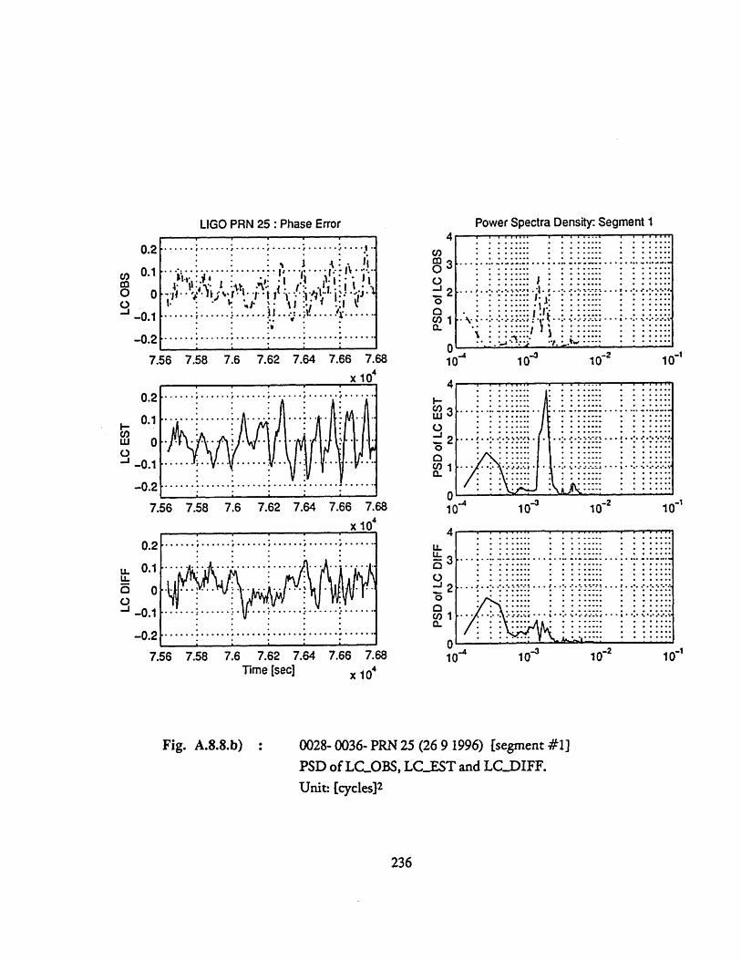
.......... ........
.
::::::::::::::
..... :..........
....
.... :....
... ...
.. ..
.....
..
..
....
... .
..
°... °.
...
.
i
,,
* '. 4.
.4
S80 0110o G
Sd
IV
C3)
C'J
V-
IS3 O
1o O
Sdtt
c) C
J
Y
>
=1i10 O1 lo OSd
* ...
.
* 3
4...
-I.--T··
··
·
0s
Io ooI
I
SG80 1
N
T- a
I-I
I-or-
... .
.. 4.
..* .
5.
... .
..
:::: ::::::::::
::::....:
... ...:
......
: :
.... •....
..........
.i .
.i .
o
...
.... ....... ..: .
........
.... ... ..
: ..
...
......'.
...;
.... .
o e
(C4 "
183 07
.... ............
..o ..
'
.o
...• ..'"
:::::: ::::::::::*::::
........
..*.** * %
....:.....•.....
...:::
:: :I : :: :
: : : : : : :
....
*
.............
........... ....
iiii~iiii
..
"0P
TIT

LIGO PRN 15 26 9 96
-60UU -4UU0 -zUUU U zUUU 4UUU 6UUU 8000
CROSS-CORRELATION between LC OBS and LC EST
-4000 -2000time delay :Tau (sec)
2000 4000 6000 8000
Fig. A.8.8.c) : 0028- 0036- PRN 25 (26 9 1996) [segment #1]Auto Correlation of LC.OBS (Roo) and LC.EST (t,).Cross Correlation be.tween them (R
Unit: [cycles] 2
237
-8000
1
0.5
~ 0o
I
2 -0.501
-8000
I 1
I I I I I I-6000
segment 1
•A

(D0LaLo
n.0,0
o0 0
0 0
U)
C
C" )
CJ
S,) S PU
e (1 0 S
0 o
C
O
V
o0 0
0o 0
0 0
l0 0
0
(1) s 10 :: rlll~dliV
000z
co c0
In,
0cliaIS3 01 / S
0 01
00 0o
OOu L
c; o
3
o
o0U
Cc;
:::: :i
: :::
•:::::: :::::::::::::
.o....o
...........
............. ......
.-.
..... ..
.... ......
o 0 .. ... ..
S .
:...... ..
-...·
.......
: ....-
!:::: :i!::::::::::::::::::::::: !
.: ..::
........:
... ...
: :
......:......
*....... ......
..............................
..........
... ...
.........
.
.................. .... ..
....
..
..
°o. o
...
...
• ........
......·.......
..... .
...
...
... .. .. .. .. .... ..
N(3
-r0S
ci30)
0u
t.
0
11O
~o I
rSUt~
,
41 Uu,0tn
00 0C
lcn
·.·
:.·;..........,,,,,
...o
... ....
o....... .............
t......................
..
.. ..........
*......
...... .....
...... ......
:•......
....
....
..
......*. ......
...... .............
.. ..•......
........ ...... ......
..
........
%......
.....
.........................
.......... .
ii ****:"•
**** ***~
•**: *
··-
·:
150i
",
··
·C
······~········
··
·-·-
C-
~··i
·~·-
.··L···~
Y~
~L
~I+
- ----
r-rr+
··i·~··.
'(·
·.-I~.-·
··
··
~-rr
-r
.-~..
·~·r:C
r,
br-c 1,O
SCR
U)

"RESIDUAL" = difference LC Observed - LC Estimated
7.7 7.72 7.74 7.76 7.78 7.8Time (sec)
o - LC OBSERVED *= LC ESTIMATED
7.7 7.72 7.74 7.76 7.78 7.8Time (sec)
Fig. A.8.9.a) : 0028- 0036- PRN 25 (26 9 1996) [segment #2]Phase residual LC..DIFF, determined as the differencebetween LC.OBS and LC.EST.Unit: [cycles]
239
7.82x 10⁴
7.82x 10⁴
LIGO PRN 25 segm #2

LC D
IFF
LC E
STo
ooC
C
>
PSD
of
LC D
IFF
0 -
C> ýn
-· in
........ ..... ....
.... .....:....::
:;..
...
...
...* *
....
. * .
....
. •
.....
:.:...
..
.···
·
···
··
·,
·
PSD
of L
C ES
T0
--C
) 0in
'
1 t
-L 0 -A 0 0
.....
...
.....
...
....
......*. .........
......
.. ...
...
;. ..
I···
...............
....
• : ..... ......
.. ..
... : ... : ....
*** : :::
: *
*:
:
**
.:
* :. • :•: • :: :
****
****
**,*
****
|***
*
LC O
BS
I I
00C
0
0O
o
oOI,. I
....
. -..
.: ''''~
.L.
•.
.·
: ..
: :
....
: .
~..•
.
: : .•
.- .
...
~'' :
.,'
...
...
-:
.·:
··:·S
,.•-"
:
:/
:
PSD
of L
C O
BS0
-4A
O
i1n
-.
i .n0 C
7T
T
7
......
...
.....
.*
....
......
.. ...
:...
... .. ...
....
... ...
..
.. ..
e
, .... ...
,
..
.
....
* ..*
...
.**
*..
..**
* *
**
**
**
I*
**
**
***,*
****,*
****4****
~i:
::ii
iiii
ir
ttJ~
0"0
0) 0 r(A"
rtI.
• ... :..... ...... = ...
1·
L
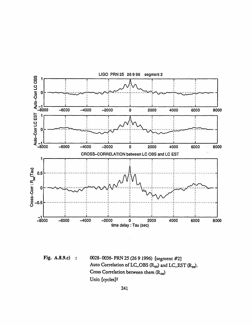
LIGO PRN 25 269 96 segment 2
-6000 -4000 -2000 2000 4000 6000
CROSS-CORRELATION between LC OBS and LC EST
-6000 -4000 -2000 0 2000 4000 6000time delay :Tau (sec)
Fig. A.8.9.c) : 0028- 0036- PRN 25 (26 9 1996) [segment #2]Auto Correlation of LC..OBS (Roo) and LC.EST (R).Cross Correlation between them (Ro)Unit: [cycles] 2
241
m 1
I0-1-800
-80
-8000
I I I I I I I
DO -6000 -4000 -2000 2000 4000 6000 BC,00
.I I . I I .
80 00
0.5
-0.5
1-8000-8000
....................................
8000
00 -6000 -4000 -2000 2000 4000 6000 80
- -r---
H
R-°
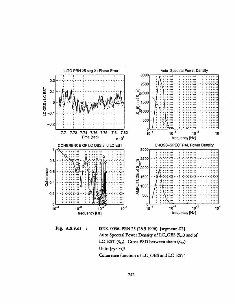
O
o O
o O
0
o w
Co
oI
I
IS3 01 /8
0
01
.... •.
.......
..
... ..
.... .
.*
....
...
-.
--.
--.-
.... .,. ..
........
.... ....... ..
.........
... ........
...... ..
... .....-..
.......
o
.....
..... ....
;..• ..
. ..:..........
U)
uiC)cu
*0C)
-iLL0wzwwx00L)4
o
C)
0 0
LO
0 I)
Co,
o ou
, o
• o
W0
(;) SJo~OflhIYdtW
e 6 eqo
eougioqoo
>8
C0a.C.
OO
1,.CCCc 8
........ .. ...
.......
....
.....
.......... ...
.. .
.. .....
.. ..
.***** *~
* .
:
..**...
* .
... .
...................
...
..
..
...
.8
.8.··
··
·:
··
; ·
··
··
·.
8
.8.::I:::i::I:::i::
:·: ·
·,,,i,.1
.8
.9
.~~
~
i
4-,-4)
U)
L.Jv,
0:c0
.'
6 6
N
d
• ... ....... .......
..
....... ......
.. .
.• ..
• .°o
..
..
..*.
,
..... .... .
...
..
...,.o ..
...
., ..
..
,
..
....
., o. ..
,
..
e
o ........
.........''
....... " ",'"
• .....
: " " :. : "
...
.. ':
: : : :
" :: .
....-.
........... ... o..........
0 0i
7 , 0 ...
....
....
00
o---
--.A
-
o
c ý -u) -!
D V
c
P
O0,-

GPS "OBSERVED" L1 :LIGO PRN 09 - Single Difference 0028 0036
.........""'......."...... ............-.............................. ............... - .............. ...... .- ......... .... .............-... ." ".....'. \
S -....................
. . . . . .I.- .. . . . . .. . .
! I ! I I
7.48 7.5 7.52 7.54 7.56GPS "ESTIMATED" L1 computed from the analysis of SNR variation
7.48
7.48
7.5 7.52 7.54Comparison L1 OBSERVED vs L1 ESTIMATED
7.5 7.52Time (sec)
7.54
7.56
7.56
Fig. A.9.1 : 0028- 0036 Satellite: PRN 09Data acquisition date 25 9 1996
LLOBS and LilEST compared for t=7.46 -7.58 104 secUnit: [cycles]
243
0.10.05
0-0.05-0.1
7.46
0.10.05
0
-0.05-0.1
S................ . ...... ......... .
I I I I I
7. 46
0.1w 0.05WI 0
0 -0.05" -0.1
7.58x 10'
7.58
x 104
7.58
x 10'
I I I. I
................ ................ .............. : ...... ................. :.
-. . ',
. .. .. .. .. .. .. .. ..
................................ .................................. ............. ..... ....................I I I Ii
7.46
. . . .. . .
.............
.............
... .........

0.15
0.1
0.05
0
-0.05
-0.1
-0.15
-0.27.4
0.15 -
0.1--
w
wa -0.05
-0.15 -
-0.27.46
LIGO 1995 9 25 PRN 09 - Single Difference 0028 0036
7.48
7.48
7.52Time (sec)
7.5 7.52Time (sec)
7.54
7.54
7.56
7.56
Fig. A.9.2 : 0028- 0036 Satellite: PRN 09
Data acquisition date 25 9 1996L..OBS and LiEST compared for t=7.47 - 7.58 10 4 secUnit: [cycles]
244
I I I I
7.x 10
I I I I I
.............. ............. ...... .. . ........
.............................. ..... .... ..... .... ,.......... .... ...... • ." ;t ....... •./ .............................. . .......... .. ... ..... ................
I.......1 I......... 1-········ 1-··---f.~ 1...~·. ..
581
587.
x10
· · · ·
·
| • •
46
c i. ·
!.. . . . .. . . . . .

"RESIDUAL" = difference L1 Observed - L1 Estimated LIGO PRN 09
I. I I1
7. 7.5 7.54 j7.5 7.52 7.54
Time (sec)
o = L1 OBSERVED * = L1 ESTIMATED
7.56
,I. 1
7.48 7.5 7.52 7.54 7.56Time (sec)
Fig. A.9.3.a) : 0028- 0036- PRN 09 (25 9 1996)Phase residual LL.DIFF, determined as the differencebetween LiOBS and LLEST.Unit: [cycles]
245
0.15
0.1
0.05
0
-0.05
-0.1
7.46 7.48
0.1
0
0.0
-0.C
-0
7.58x10⁴
.1 .....
5 ......
0 .
5 ......
.1 - -.....
I. I I i I7.46 587.10
x 10"
1
i
,,
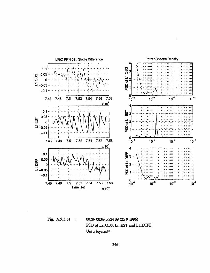
LIGO PRN 09: Single Difference
9 ..... .
S...... ..... ...... .. . ..
......... .. .. . ....
7.46 7.48 7.5 7.52 7.54 7.56
4
-J0
0,I._aCl
,.
7.58x 10⁴
7.46 7.48 7.5 7.52 7.54 7.56 7.58
x 104
0.050
-0.05-0.1
7.46 7.48 7.5 7.52 7.54 7.56 7.58Time (sec]
n
Power Spectra Density
10- 10-2
10" 10" 10-2x 10
Fig. A.9.3.b) : 0028- 0036- PRN 09 (25 9 1996)PSD of LLOBS, LL.EST and LIDIFF.Unit: [cycles] 2
246
0.10.05
0
-0.05-0.1
.i
I..:::
0.10.05Co
w O" -0.05
-0.1
X- r
fAf.. ......- ...... -. .....: .. .... * .. . . . . ..... 1
. i . . . .
10
10'
_ _____:r _ · · · · I··
. .. . . . ..-. . . .
i
. . .. . . ., .,, . ...... I
·- ·. ...........
.... ... ...... .....
.. ......
I10l
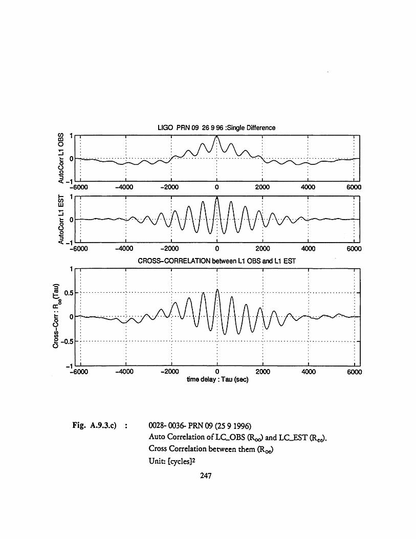
LIGO PRN 09 26 9 96 :Single Difference
-2000 2000 4000
CROSS-CORRELATION between L1 OBS and L1 EST
-2000time delay: Tau (sec)
2000 4000
Fig. A.9.3.c) 0028- 0036- PRN 09 (25 9 1996)Auto Correlation of LCOBS (Roo) and LCEST (Ree).Cross Correlation between them (Roe)Unit: [cycles] 2
247
0
wcIn-
-J
0C.,J0ro<•
-4000 -2000 0 2000 40006000
-6000 -4000
t=.
OIeA
6000
e -0.5
4
. . . . . . . . . . . . . . . . . . ...... ... . . ... . ... .. . . .
-I
-6()00 -4000 6000I
mA =41
-,, 3- 6000

Auto-Spectral Power Density3000
2500
150C
81000500C
7.46 7.48 7.5 7.52 7.54 7.56 7.58Time (sec) x 10'
COHERENCE OF L1 OBS and Li EST
10e 10-Z
frequency [Hz]10
- 1
300C
. 250C
-) 200C0
150C
100(Ca.
C50
10 10-2
frequency [Hz]
CROSS-SPECTRAL Power Density
.... :... . . ... ..
10- 10-2 10- 1
frequency [Hz]
Fig. A.9.3.d) : 0028- 0036- PRN 09 (25 9 1996)Auto Spectral Power Density of LC_OBS (Soo) and ofLC_EST (See). Cross PSD between them (Soe)Unit: [cycles] 2
Coherence function of LC_OBS and LC..EST
248
0.15
0.1
0.05
0
-0.05
-0.1
I i -
i. f. *1.IF. ~.
: -:--.::::: -: - .::::::: : : : ::::::: :. ::::: : :: : : : : : : :
1 i ~iiriiii i" ii ii i i iil1.~ .~... . .\..--
L -· .- .j
10-1
0.8
0.6
0.4
0.2
0
10-4
I
--
10l
. " .. . ' . . ... ..
• " ' .. . . . .. ... .... . . . .
. .. • .. . . . . ...
'
"''
L.
10-
LIGO PRN 095:L1

GPS "OBSERVED" L2 : LIGO PRN 09 - Single Difference 0028 0036
7.48 7.5 7.52 7.54 7.56GPS "ESTIMATED" 12 computed from the analysis of SNR variation
0.
-0.
-0.:
0.
0.
-0.
--0.
7.56
7.5 7.52 7.54 7.56Time (sec)
Fig. A.9.4: 0028- 0036 Satellite: PRN 09- Data acquisition date 25 9 1996Lz_.OBS and Lz.EST compared for t=7.467-7.58 10 4 secUnit: [cycles]
249
0.:
7.5 7.52 7.54Comparison L2 OBSERVED vs L2 ESTIMATED
.. .... ... ..... ....... ...... .1 .\. . :.. . . . .. . . .... . ...... ,: ....... . .. . .. ... ... ;.
S'• ; : ii : I
I I I I
2
1
0
1
27.
2'7.
7.xiO
2
1
0-
1
46
46
58t
.584
7.48
7.48
0.2
0.1
0
-0.1
-0.27.
7.
x 10
I . . ~ Il I
7.
x 104
·
· · · · · 1
i
46
58

LIGO 1995 9 25 PRN 09 - Single Difference 0028 0036
7.5 7.52Time (sec)
7.54 7.56
Time (sec) x 10
Fig. A.9.5: 0028- 0036 Satellite: PRN 09Data acquisition date 25 9 1996Lz.OBS and LEST compared for t=7.47 - 7.58 10 4 secUnit: [cycles]
250
0.2
-0.1
0_
...................... .. ............. ...... .. ......... .. ................... .............
I I I
7.46 7.48 7.58
x 10'

"RESIDUAL" = difference L2 Observed - L2 Estimated LIGO PRN 09
7.48 7.5 7.52 7.54 7.56Time (sec)
o = L2 OBSERVED * = L2 ESTIMATED
7.48 7.5 7.52 7.54 7.56Time (sec)
7.58x 10
Fig. A.9.6.a) 0028- 0036- PRN 09 (25 9 1996)Phase residual L2zDIFF, determined as the differencebetween Lz.OBS and LzEST.Unit: [cycles]
251
0.15
0.1
0.05
-0.05
-0.1
-0.15
_n-'..
7.'I I
7.58x 10'
0.2
0.1
-0.1
-n o7.46
S ............. .............
F . .
B .
46
- .. .
I-
i_ .....-

LIGO PRN 09: Single Difference
cn 6mO
o0
n 2a.
7.48 7.5 7.52 7.54 7.56 7.58x 10'
7.48
10 4
6
0co2CL.
r7.5 7.52 7.54 7.56 7.58
x 10'
7.48 7.5 7.52 7.54Time [sec]
Fig. A.9.6.b)
7.5(
u- 6u-94o
02
6 7.58
x 10'
10-4
Power Spectra Density
: :...: . ........ . ......: o o -. .. ... • o. .
· · · · · · · · : i ii i i'ii'iiiil
~..:::J :.• • ... °° ° • . °... . o • .oo,': : :::::::l=
10
10l
10-4
10-2 10-'
10-210 10
10-2
0028- 0036- PRN 09 (25 9 1996)PSD of LC.OBS, LC..EST and LCDIFF.Unit: [cycles] 2
252
0.1
-0.1
_A' #
i
...... ..4.. . ....
... ... .. . .. I. . i " s,i j: I··l jt '' IJ '''V
,- +A-VV- V - \ -- -- - --
7.46
-0.1
0n
7.46
0.1
0
-0.1
-n o
"· " " ' " ; ;1 " . ..' " " " ' '
: ; ::'• i::; : : : ::
7.46
/ : :::::: : : ::::: : : ::: *1
10-'
I
I i I I l i
@ I i I I n
·· ·
'
*
0.2
'

LIGO PRN 09 26 9 96 :Single Difference
O
o0
-t
't
0
-4000 -2000time delay : Tau (sec)
2000 4000
6000
6000
Fig. A.9.6.c) : 0028- 0036- PRN 09 (25 9 1996)Auto Correlation of LC..OBS (Roo) and LC.EST (Re).Cross Correlation between them (Roe)Unit: [cycles] 2
253
-6000 -4000 -2000 0 2000 4000
CROSS-CORRELATION between L2 OBS and L2 EST
6000-6000 -4000 -2000 0 2000 4000
oI0U
0.5
-0.5
-1
i I I I I I
I I I I -- I I
-6000
Ii i i i i i
-

LIGO PRN 095 :L2
7.48 7.5 7.52 7.54 7.56 7.58Time (sec) x 10'
COHERENCE of L20 Bs and L2EST
frequency [Hz]
CROSS-SPECTRAL Power Density
0.8
0.6
0.4
0.2
Atio-4 102-
frequency [Hz]10- 1 10. 1-0 10- 2
frequency [Hz]
Fig. A.9.6.d) : 0028- 0036- PRN 09 (25 9 1996)Auto Spectral Power Density of LC_OBS (Soo) and ofLC..EST (Se). Cross PSD between them (Soe)
Unit: [cycles] 2
Coherence function of LC.OBS and LCEST
254
.,,...tI-I.
0.2
0.1
0
-0.1
0A
7.46
10-I
Auto-Spectral Power Density
·
0%k r.f P£•f%
···· · · · ·· ·· ···· · · · ·· · ·· ····· · · · ·· ·· ····· · · · · ·· ·· ····· · · · · · ······ · · · ·· · ···: · ··' ̀ ·'·` =-·~i '·':''·' =`·';·'·::···· · · · ·· ·· ······ · · · ·· ·· ···· · · · ·· · ·· ··· · · · · ·· ·· ··· · · · · · · ·~·.·..·······.·2\ · · · 1····t··. ·. · · · ~~·
· · · · · · · · · · · ·· · · · · · · · · · · ·
· · · · · · · · · · · · ·"" · · · · · · · · ·· · · · · · · · · · · · ·
· · · · · · · · · · · ·· · · -··' ""' · · '·'···-···~L··~
· · · · · · · · · ·· · ·· · · · · · · · · · · · ·· · · · · · · · · · · · ·
· · · · · · · · · · · ·"" · · · · · · ·
"· ...."· ' ' """'
"'· ''"
'V'' UY"
'
·'
·'
10 410-2-10

90 90
270GPS DATA: receiver location: SOUTHERN CALIFORNIA acquisition date: 23 1 1997
station: COSE (trimble) satellite: PRN 01
Time (sec)
200
• 150
100
6x 10⁴
station: COSE (trimble) satellite: PRN 01
Time (sec) x 104
Satellite visibility chart for PRN 01 (skymap).Elevation and azimuth of PRN 01with respect tothe station COSE
255
100
Fig. A.9.1 :
)
* !............ ............. .............. ......... ..... .....--- ........ ..... .
0

COSE (trimble) PRNOI 2311997
5.54.5Time (sec) x 104
Signal to Noise Ratio for L1 and L2
I I IIIII II I. . .. . .. . . . . .. . .. . . .. . .. . .. . .. . . . . . .. . . .. . .. . . . . . . .. ... . . . . .. . .. .. . . . . . . .. . . . . . . . . . . . . . . . . . .·· · l · `---~'
3.6 3.8 4 4.2 4.4 4.6 4.8 5 5.2 5.4 5.6
I - - I--- : -- I - -- I -:I:I S I I
3 .6.8.. .. .. . . ........ . ... .
3.6 3.8 4 4.2 4.4 4.6 4.8 5 5.2 5.4 5.6Time (sec) x 10
Station: COSE - Satellite: PRN 01Data acquisition date 23 1 1997Signal-to-Noise-Ratio (SNR) for Li and Lz.
256
I I I I
I I
3.5
100
50
320
~10
0
20
Fig. A.9.2 :
· 1 ·
i I
_r
COSE (trimble) PRN 01 23 1 1997I |
I
. ..............-
I-

GPS "OBSERVED" Phase Residuals for: COSE (tr) PRN 01 - CALIFORNIA 23 11997
3.6 3.8 4 4.2 4.4 4.6 4.8 5 5.2 5.4 5.6GPS "ESTIMATED" Phase Residuals computed from the analysis of SNR variation x 10
3.6 3.8 4 4.2 4.4 4.6 4.8 5 5.2 5.4 5.6Comparison LC OBSERVED vs LC ESTIMATED x 10
3.6 3.8 4 4.2 4.4 4.6Time (sec)
4.8 5 5.2 5.4 5.6
x 10
Station: COSE - Satellite: PRN 01- Data acquisition date 23 1 1997The observed phase residual (LC.OBS) is compared with themultipath phase error estimated from the SNR (LC..EST)Unit: [cycles]
257
-.... .... ... ......... . ......................... ......... ........ ... ............... ... . . .... ; .
...... .... ............ .................... ..... ....... .... .................... ......... .. -, • . '
0.2
0
-0.2
-0.4
-0.6
-0.8
0.2
0
-0.2
-0.4
-0.6
-0.8
0.2
-0.2
O-0.4
- -0.6-0.8
,... ........... ,I......r.....l..... ........ J........ !..
.-.~... ... t....................--:
.. .. .. .. .. .. .. .. .. .. ..* .. .... ........ ........ ..: ~
- ··! · · · ........ ....~·· ·· ·! · ·· · ·!· ·· · ·a · ·· · l· · ·
. .. .. ... .. .. ... .. .. ... . ... .. . ... .. .. ... . ... .. . ... .. ...
Fig. A.9.3 :

COSE (trimble) PRN 01 - SOUTHERN CALIFORNIA 23 1 1997
3.6 3.8 4 4.2 4.4 4.6 4.8 5 5.2 5.4 5.6Time (sec) x 10'
3.6 3.8 4 4.2 4.4 4.6 4.8 5 5.2 5.4 5.6Time (sec) x 10'
Station: COSE - Satellite: PRN 01Data acquisition date 23 1 1997LCOBS and LC_.EST compared for t=3.5 - 5.7 10 4 secUnit: [cycles)
258
0.2
a
-0.2
-0.4
-0.6
-0.8
0.2
0
-0.2
-0.4
-0.6
I i I I I I i I I I. . ........ ......•o ., ,. ,, • .. . o, , o o , , ................ o-,- .....•o .. o ......... o'o
" '
... . . . ... ....... •......... ........ ............. . ._..... .. ... ..•· · · ·· · · .·· · · ·· ·
~~~·~····:· :''''~'''' i~''`' :' t''' · ·''~'·''
.. .. . ,.. .. .. ., .. . .. . ,. . ... • .. . . .,,. . . .•. . . ., . ,. . . . , . ° . .. . .
Fig. A.9.4 :
3.6 3.8 4 4.2y.o

"RESIDUAL" = difference LC Observed - LC Estimated
3.5 3.55 3.6 3.65 3.7 3.75 3.8 3.85 3.9 3.95 4Time (sec) x 10'
o - LC OBSERVED (COSE 01 trimble Part la) * LC ESTIMATED (COSE 01 trimble Part 1 a)
3.5 3.55 3.6 3.65 3.7 3.75 3.8 3.85 3.9 3.95 4Time (sec) x 10
Fig. A.9.5.a) : COSE - PRN 01 ( 23 1 1997) - [segment la]Phase residual LCJDIFF, determined as the differencebetween LC.OBS and LCEST.Unit: [cycles]
259
: Part la

...
..
%.t..........
..
• ...
........o............
ii
i'
•%
....... ..
...... ...... ..
....
...
..2. .
........
2.
......
..
... .
*.A
···
·i ··
·-·
* -S
··.
2
.···'··'· ·
I:···
S0 0
01 Sd
SBO
0"I lo (•Sd
I ..:
: 1
Ile:
:/•
•..-•
H~
HI
KŽ
l I
I _
IN
'-
o r-
N
0o 0o
SGO
31
00 (D
It
N
C
IS3
110 lo
Sd
N
r o
r-
oSo 31
:........J............::::{::ii:::•"
::
..........................
:::::
.....,.....
% ..........
S......
..:..
.-
...!....z
. ....~. .•.
.... ; ....
;. ...3•.
cc
co
oD
o
t C
%
C)
,6 o
o o
=1i0
31o
0 CISd
1-0la 01
.........:...............I
o ..........
.... ....
............
................
.... .;..... ...
2.J
vjEP
,
1=·
*
.U,
,1o-4
C/)
QO
'0 u9I..z1 o
eeb
0c
t
.........
•-............
,•,
•
.,.,
~
·~···~·-····-·-
~····I ·
··
4r·····s·5· ·
··
·I
I I

COSE (trimble) 23 1 1997
-2000 2000 4000
CROSS-CORRELATION between LC OBS and LC EST..... I
time delay :Tau (sec)
Fig. A.9.5.c) COSE - PRN 01 ( 23 1 1997) - [segment la]Auto Correlation of LCOBS (Roo) and LC_EST a(t).Cross Correlation between them (Ro)Unit: [cycles] 2
261
F·v
C,
0
oo
-1
-60
w
0O0I
-60
604-4000 -2000 0 2000 400000
00 -4000
00
00
0
2o
o0I
U,LO)
00
60
0.5
0
-0.5
_.
-6000
.............. .......... o.......................
.. . . . . ... • . . . . . . . . . . . . . . . . . .
-4000 -2000 2000 4000 6000
segment la
S..
.. . .. . . .. .. .. . .. .. . .. . . .. . . . . .. .....
. .. .. .. .. .. .. ..

Cohe
renc
eO
JE
0
LC O
BS
/ LC
EST
o CA
)
L"
RC
A) in
CA
(D eut
AM
PLIT
UD
E of
S,(
f)(
Co
m
o
O01
o 0
o o
o 0
.. ...
......
...
..
...
....
....
...
....
....
. ....
... ..
...
..
..*
.
..
..
.....
a .
.......
...........
..........
...........
°
.. .
..
...
....
....
....
.
.. .
.
......
...
........
......
X
......
I....
* ...
..:
...*
...
I.
.:
.:
......
-L
o K
o0
00
-&
i
Soo(f
) and
S (
f)01
o
01
0
010
0 0
C
0
-L "1
-LI 11
34
n.
0
0 a 0 -'-a
*o 01
-L 0ii
.....
.....
....
..
.. .....
...
.. ...
.. .......:,
........
.....
..
"
, ."" .... .
*..... .. ..
S,-...
..
..
' ..
.'
''
''
.* .. . ......
*.......*%......
..........
......
....
I:::: I: : ::
: I ..
......
....
: :
I
I>
%..
-L
o0h

"RESIDUAL" - difference LC Observed - LC Estimated
4.1 4.2 4.3 4.4 4.5 4.6 4.7 4.8 4.9 5Time (sec) x 10
o - LC OBSERVED (COSE 01 trimble Part Ib) * LC ESTIMATED (COSE 01 trimble Part Ib)
4 4.1 4.2 4.3 4.4 4.5 4.6 4.7 4.8 4.9 5Time (sec) x 10
Fig. A.9.6.a) COSE - PRN 01 (23 1 1997) - [segment Ib]Phase residual LC.DIFF, determined as the differencebetween LC.OBS and LC.EST.Unit: [cycles]
263
0.1
0.05
-0.05
04
4
: Part lbA =

I o io
o CO
oo
10
Ct,)
0 0
00
-&
r O
PSD
of L
C D
IFF
Do
m
0 .A
.
° .o .....
o°
o.....
%..
.....: .....
.. .
,,
, .
....ol.....
...
... ....
o l e
e
....
......
...
..
....
.
..,o .. .... ..
•..
,..
• ..
i .
i ....... .
. .
.:::::::i :::::::::::::
....
...
....
...
.
....
• .....
• ...
. ...
.a.%.,..,,,,
...t
...
..
..
....
..'·
···C
'''"
.4
0
PSD
of L
C ES
TCo
tr c
J .0
....... ........ ...
....... ..
o
.
... ......
............ ....
....
•.....
....
..
•.
.
..... •...
.. •..... 0. .
....
... ...
.... .. ..
..
.iiii
iiii
i.i.
..i iii
.... ,i..... |
... ... I. .
PSD
of L
C O
BS
O
rA
C# 3
......
..:..
.....
•o ....
... .°°• .
°.
%..,
.°e••.. °....
..
I ..
.•
: .:.
...
...
...
..
... .
.o. .
..
., .
...,.
....
. ...
... .
.. ..
. ..
.. .
..
, ..
.... .
...
, ,
•
...
.....~
~
~ i .
.. i .
.. I.
.
LC D
IFF
LC E
STo
o u
LC O
BS0
0
01
'. -.4 C g-
03
'b1.
0L-0&
u
L

COSE (trimble) 23 1 1997 segment lb1
0
-1-1
-1 -0.8 -0.6 -0.4 -0.2 0 0.2 0.4 0.6 0.8 1
CROSS-CORRELATION between LC OBS and LC EST x 10
-1 -0.8 -0.6 -0.4 -0.2 0 0.2 0.4 0.6 0.8 1time delay :Tau (sec) x104
Fig. A.9.6.c) : COSE - PRN 01 (23 1 1997) - [segment lb]Auto Correlation of LC.OBS (Roo) and LCEST at,.Cross Correlation between them (RUnit: [cycles] 2
265
___ I I I I I ~ t I ___-0. -0.2 0 0. 0. 0. 0.06
-.
03m
Ot-
O
0II--
.. I
o
O
I
-0.2 0 0.2 0.4 0.6 0.8-0.8 -0.6 -0.4

o 0
0
(f)l 0Spue ()°s
o 0
..... ..... .
... ... .
.... .. .* .*.
..........:::::::::::::::::::............
.... ...
.................... ....
.........
...... ........
o%
U,
0CL
-o00C
L0..
0)0.I0
U)
womC)
co
00C/)
c oozcr0
IIS
3 01 / S0O
31
o
0o
oo
oCt
C)
(I) S lO 3E
inldnidVV
c o
oeouo.otoo
...: ....
................. ···% .°,,
..0°
.......
o0
o• °..
.
,,.,,o,,,,,o,,,,,,,,,,,.,,,,,,,
..... :
.. .
.. ......
*......
*......
...... .
.... .
.... .
..... ... ......
....
... ,...
..
,
..,...
... .....
............. ....
..............
.*.
..... .....................
........... ...
.. ...
..
.... .
.. .
...
... .
..
... ..
...
.: ..
..
.. .. ..
..
.. .. ..
..
..... ....
... ....
...
....·.....
00,0o·r0
ccCC
(CN
-1-p
-.I:c)
C")0*c1
'440
r--
0--
C/
04C0.=
U
-e
T-cr(0
I i
--•
I
I I
| I
cCc
(3·.€
ov-!
....
,:......
,- ,
,
-|-.,-.-: o
-,
::: ::::::::::::::: :::::::::
.......
..... ........
....
............ ......------
----- ------
-----
......
.......... ......
...::.............. ..
........ .......
.o
, "
.. .....
•...... *...
• .
•····
c
a0
,-ks it
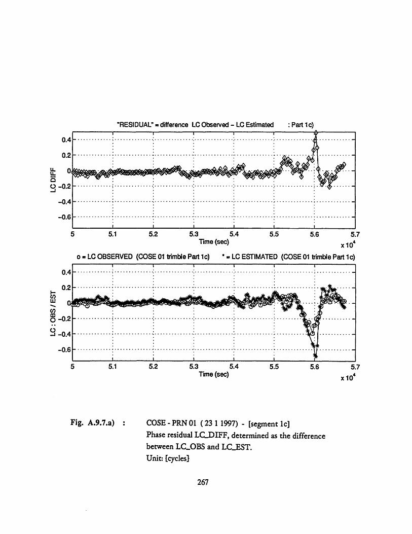
"RESIDUAL" = difference LC Observed - LC Estimated
5 5.1 5.2 5.3 5.4 5.5 5.6 5.7Time (sec) v An
o - LC OBSERVED (COSE 01 trimble Part Ic)
A IU
* - LC ESTIMATED (COSE 01 trimble Part 1 c)
5 5.1 5.2 5.3 5.4 5.5 5.6 5.7Time (sec) x 10'
Fig. A.9.7.a) COSE - PRN 01 ( 23 1 1997) - [segment 1c]Phase residual LC..DIFF, determined as the differencebetween LC..OBS and LC.EST.Unit: [cycles}
267
: Part lc)

L" .
.• t • • • •
..
..
.. ..
...
.. .. ......
:..::::::: ::.
.............. ,
...... ....
" .... ....
....:...............
.1.e
0Cl0
17Cl
T-
0 Bco
7 o cm
oSG
O 31o0 aS
d
..............:::::.::::.:::::.::::
S
..
..
..
...
...................
oo
Co
0
m
C1S3 0110 O
Sd
%
..
.........
................
..........~.....,
-o CD
IV
C
O
IOla 31
1O GSd
J~
.,
...
o o
o
o*1
r
/"~""
I$'4
to D
3o
O
O;
I~o
Cu
lIn
31110 31
9u
0C
/)e
U9,.. g
' P1°\
w0DU)
-ca-zcca-wCl)aOo
.0)a)
E1=
5
IS3 01
gh
I•g
I ..
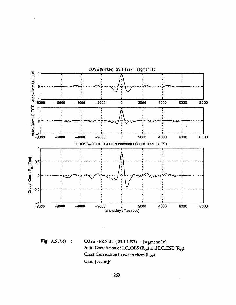
COSE (trimble) 23 1 1997 segment 1c0e -
-6000 -4000 -2000 0 2000 4000 6000
-6000 -4000 -2000 0 2000 4000
CROSS-CORRELATION between LC OBS and LC EST
4-I
-8000 -6000
Fig. A.9.7.c)
-4000 -2000 0 2000 4000 6000time delay :Tau (sec)
COSE - PRN 01 ( 23 1 1997) - [segment Ic]Auto Correlation of LCOBS (Roo) and LC_.EST (Ree).Cross Correlation between them (Roe)Unit: [cycles] 2
269
0co0O
o
0
-•-000I--
U)
o-IoI
.2
8000
8000-8000
L.
0
c Oo
o0,
- -0.5o
6000
8000

..t-CL.0)
a,0.(I0
X :: :*:
: ::ý ::
-::::................
·.......... .
.............
; ...
..
.
..........
................................ ..... ·.....
~. ... .............
X..
..
... .
..
.. .
..
..
..
....
.oo .
...
...........
lo
..
... .. ..
o
..o .. .o
o. ...o .... ..
:
1 o
d
d C
D
oI
I I
I
IS3 01 /80
01
I0
0 0
0 0
W
0w
0 0 9
(I) S lo
:l(l'lldVV
_I-V
X
OWcm
, )
So
n
0
ui
LI
00It
-CO
D
.
e o o0
C)
0V-
NNX0CD0):30*~
.• ..,
..°. ....
.°
....... .
•.
°
..,.....
......:......
...... .....
..:......
...... ......
...... ......
......
..
•.
.... .
..
..... .
.Z...,,..
....
...
........ ..... ...
.... ..
:.
.::::: :: .. ..... ...
.:
.o,....·.
..o .... ....
.... .
.. .
... ... .
..
... ... .
...
: ..
... ..
.. ..
..: .
..
....
...
...
...
...
...
... ..
.. :
..
..
..
..
·.
....... ....
cuIc120
a*
Sco
oo0
0o
0 0
0cCii
2LU
0a.U)
CY
u(DE0,0aa,B,2,wC
'0e0
J
0
I 0
c 0'o4
03u-eC
i4
j1
U4
8
| li
I
: .::::......
...
....
...
::::'::.::: :
......*...........................
.. .
.. ...
.. .... .....
........·.... ......
,.....
......
.............
......
i i
i
I
i
I
>>
{g
o T
-
Io
0 ,-
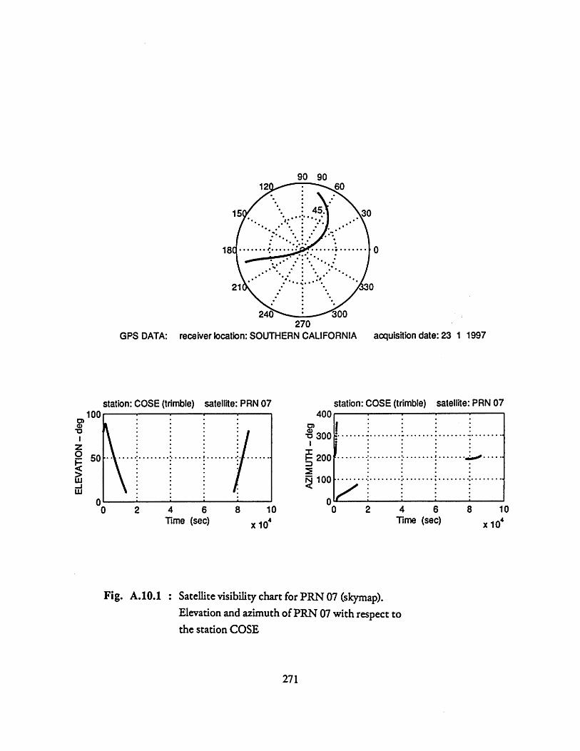
90 90
270GPS DATA: receiver location: SOUTHERN CALIFORNIA acquisition date: 23 1 1997
station: COSE (trimble) satellite: PRN 07
0 2 4 6 8Time (sec)
10x 104
400
S300
200
100
00
station: COSE (trimble)
2 4 6Time (sec)
satellite: PRN 07
8 10
x 104
Fig. A.10.1 : Satellite visibility chart for PRN 07 (skymap).Elevation and azimuth of PRN 07 with respect tothe station COSE
271
1
0,z0
w
I †
................ 7
........ .......... ...............e000010 ····~····(····s~~~~·
1
· ·
0
A

COSE PRN 07 23 1 1997
1 2 3 4 5 6 7 8x 10⁴
Signal to Noise Ratio for L1 and L2
Time (sec) x 1o
Fig. A.10.2 : Station: COSE - Satellite: PRN 07
Data acquisition date 23 1 1997Signal-to-Noise-Ratio (SNR) for LI and L2.
272
100
30
20
Z10
0
z 20
SI I I i I I.
. ... ... .. . . ... ... ... .. .. ... ... .. .. ... ... .. . .. .. ... ...
1 2 3 4 5 6 7 8
Ci
-- A m A
I I I I I
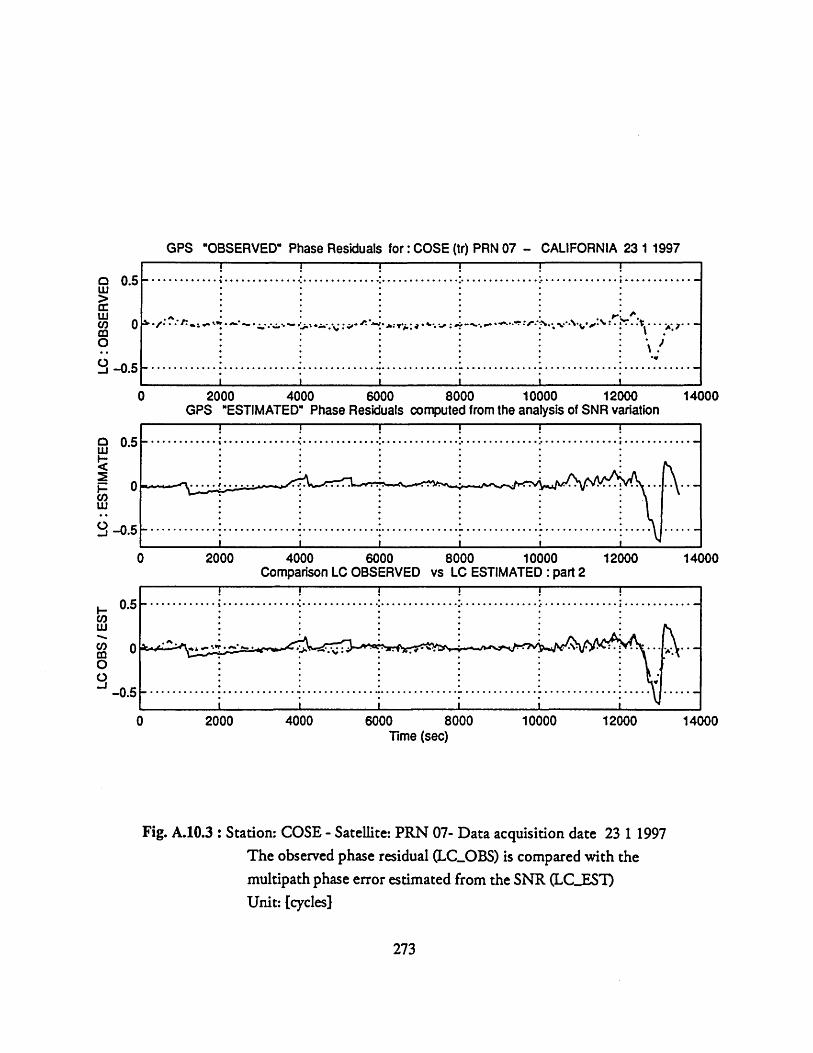
GPS "OBSERVED" Phase Residuals for: COSE (tr) PRN 07 - CALIFORNIA 23 1 1997
0 2000 4000 6000 8000 10000 12000GPS "ESTIMATED" Phase Residuals computed from the analysis of SNR variation
0 2000 4000 6000 8000 10000 12000Comparison LC OBSERVED vs LC ESTIMATED: part 2
2000 4000 6000Time (sec)
8000 10000 12000
Fig. A.10.3 : Station: COSE - Satellite: PRN 07- Data acquisition date 23 1 1997The observed phase residual (LC.OBS) is compared with themultipath phase error estimated from the SNR (LCESIT)Unit: [cycles]
273
5o 0.cO
w
0
S -o.
. ............ .......... . . .............. .............. . . ............ . ............. ...........
0.5
0
-0.5
. ............ ...... ...... . * ......... .. : .. •. ......... ..... ........ . ...
I I ! I l IQb'······· '5······ · · · · · · · '2· · · ''·····
. ...... .. ........ .... *.. ........ .... *...
14000
14000
14000
I

COSE (trimble) PRN 07 - SOUTHERN CALIFORNIA 23 1 1997
2000
2000
4000 6000
4000
8000Time (sec)
data set : part2
6000Time (sec)
8000
10000
10000
12000 141
12000 14(
000
00
Fig. A.10.4 : Station: COSE - Satellite: PRN 07- Data acquisition date 23 1 1997LCOBS and LCEST compared for t=0.0 - 1.4 10 4 sec
Unit: [cycles]
274
............ .......... .......... ......... ............:.........~.............=... ........... ......
.... ... ... ... ... ..I .I. I. II .I II II .I I. .I. ..I III I.. III III III
I .I I . I I I II II II II II II II I I I I I I I
I ... IIIIII
. I .I..I .. I.. . .. I. I . . ...... IIII..I..
0.6
0.4
0.2
0
-0.2
-0.4
-0.6
0.6
0.4
0.2
0
-0.2
-0.60~4
. .... ...... .:-•. . . . ...... ............. :.............. .............. . ............. . ............
IIP• ,. : -- ** - -- -- - :-- - - -- - - :-- - - -- - : "-- - - - .*"--- ,- "\ - 9- - -
I I I I 1 'I III III II. III III .II ..I III III IIII II II II J III III III I II III .II
)
ii
)

"RESIDUAL" = difference LC Observed - LC Estimated
Time (sec)
o - LC OBSERVED (COSE 07 tr Part la) * = LC ESTIMATED (COSE 07 tr Part la)
70000 1000 2000 3000 4000 5000 6000Time (sec)
Fig. A.10.5.a) COSE - PRN 07 ( 23 1 1997) - [segment la]Phase residual LC.DIFF, determined as the differencebetween LC.OBS and LCEST.Unit: [cycles]
275
: Part larrr

F7T..T~ThT1
.1
.. .
...° ......
....,.....
..... .....
%
: .'
....;...............
..
.•.... ...... .. :
•
..•..f...~·~·
N
IL
-If
w
SO80 01 JO0Sd
S8O 0
oCD
a0Coof-%
N6)
1S3 0 j0o aS
d1J10 017 lo 0S
d
000Co
000 o0ooO j
O %
IS3I
18S1 01O
JIO 01
I40O
en
0-EF000
0

COSE (trimble) 07 23 1 1997 segment 2a
2000 4000 6000-6000 8000-4000 -2000
-6000 -4000 -2000 2000
CROSS-CORRELATION between LC OBS and LC EST
-4000 -2000 2000
Fig. A.10.5.c)
time delay : Tau (sec)
COSE - PRN 07 ( 23 1 1997) - [segment la]Auto Correlation of LC.OBS (Roo) and LC.EST (Re).Cross Correlation between them (Roe)Unit: [cycles] 2
277
03ca 1in00-jt 0*00I
.2: -1
-80(i-LU-- I
-80
I I I I I I I
I I I I I I
4000 6000 8000
I° ............
........... ......... .v ..............--0.5
-6000 4000 6000 8000
00
·
O0
t
2000 4000 6000
.. . . . .
......... ,... °°.°.o... ............. . ........ .
.. .. . .. . . . . . .. . . . . . . . . .. . . . . . . . . .
. .......... .......... ° . . . . . . . . . . . . .. . ... . . .
-8
-8000L

o 0
0 o0
o o
C) C
.. .0
o ..o....... .o.00
..o.. .
o.
...
...... ... .
... .
.... .
... ...
.....
.........
..
..
.. %
. .
......
.... ....
.... ..
..,
..
.......•......
.......
.......•......
....,•
..
.
..°. ..
..
°. °. .. ..
°.
..
°.°.°.°.
..
'"
" "° °°° °°°
°° °°°t
°°,
°°° °,°
·o·o
··°,······f°·o··
,o·····,·,°,
°,,.,°,° °.,os,° .°°•o,°o
°°o°°°
• °°°°.'
,,°*o•°
,,°,t°,
°°° °°
u)0a.CL
0L-
Q.
O)~I
C,)
0:3
CccuCC4L
IS3
0" /SBO
31
U)0a.ccwoa.OIC),)
0c:()
))
Sd do
eoueJeqoO
CY
N0
°............. *°°°
......
..
o.. °.
.° .
.....°
.%....
o,
6
%.
,
,
.....
'
..............
...
°°o°~
~~
~~
..°°
..... .° ... .. ..
°°°
.............
°
.°
°
,
..
..°°.
..
..
..
.... ..
.J.
..
.
....
... .
..
... ... .
...
..
.... ..
...
.. .
..
C
I-0
)C)O C)
C)
C-
o
S 0o
o:inlald VY
0o
o o0
o
o0U40
wa)
Cu
CtJ
E0)wC)
zcca.wcI00
0
3:>
3,C
............ .....
=..=.....
.......:...... %
..............
......
...... :.......• ...... •. .
.. : .
..
.
.............
..
..
.....
...
......
..
...
....
.....
o..
............
...... • ........ ....
...
... .
...
...
,.......•I.
..
....
..
....
....
.......
...
..... .
.. ...
...
..........
........
...... ...
..;
~.I...~
~.2
...~.
~ ..
.''''' ~~r
~ ·
··
··
05.-
P
o
(6)0,S pue
(W)"VS
I I
I I
(g
h:
c
'Ios-
(

"RESIDUAL" = difference LC Observed - LC Estimated
0.9 1.2 1.3Time (sec)
o - LC OBSERVED (COSE 07 tr Part Ib) * LC ESTIMATED (COSE 07 tr Part Ib)
0.4
0.2
O0
-0.2
-0.4
-0.6
0.
0.4
0.2
-0.2
-0.4
-0.6
0.Time (sec)
1.2
1.
x104
1
x 10
Fig. A.10.6.a) : COSE - PRN 07 ( 23 1 1997) - [segment Ib]Phase residual LC.DIFF, determined as the differencebetween LC..OBS and LCEST.Unit: [cycles]
279
7
0.9
.I I I I I
. ............ ............. ..... ..... ... %...... .............. ....... o.•.% . .. .. . .. ... .. .. .. .. .. ..
............. .............. * .............. .. ........... .... ...... ......
I I . . . I
. . . .I .. I I............................... ............. ............. ............''
. . .. . .. .. . .. . .. .. . .. .. . . . . . . . . . . .
7
.4
.4
I II • | • •
............. ............................ .. ............%~·
-·········(···· · · · · · · · · · · · · · · · · · · · · · · · · · · · · · f · · · · · · ·ile·
.... . . . . . . . . ... .** . . . . .. . . .
n I I I I I I
: Part lb
iI

.I.
.........
..................
.....I....,....
......
..................
................
.....:...
.....
.........
,.. .:..
..•...
...
...
.. ...
.
S80 031
o OSd
I
............·
··
·
:::::::~:::::·::::: :
....
................
oo..e...............
....:. .....
.........
.. .. ... ... .
..
..... .............
.
co co
0" C
m
o>
IS3 01O
c1Sd
Il 0o
) In
0
tuc
ci c;
5I
I
..7....·..·;........
.....................·.....
.. .. .. .. ..
..........
······... .......: ....
......
.....
...
......
.......
....... .......
.
to
o 01
rl 3
(58
80 0
7IS3 07
4)uuF
uII
gg
J11 01 10 O
Sd
"ki
cocii=...
aO
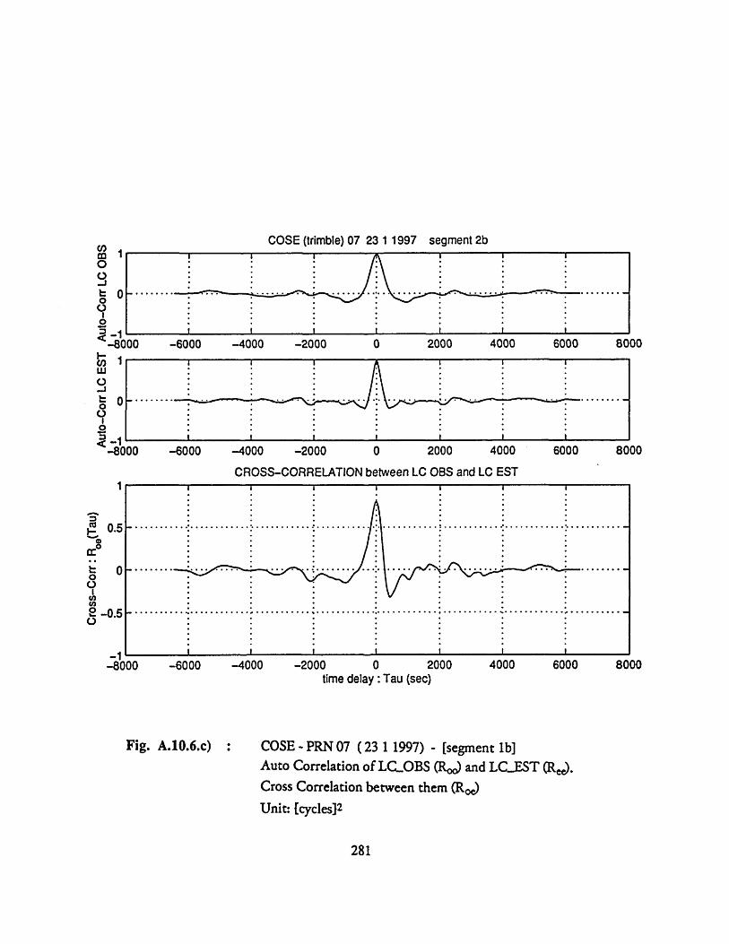
COSE (trimble) 07 23 1 1997 segment 2b
-6000 -4000 -2000 0 2000 4000 6000 8000
-6000 -4000 -2000 2000 4000 6000 8000
CROSS-CORRELATION between LC OBS and LC EST
-6000 -4000 -2000
Fig. A.10.6.c)
time delay :Tau (sec)2000 4000 6000
COSE - PRN 07 (23 1 1997) - [segment Ib]Auto Correlation of LC.OBS (Roo) and LC.EST (Re.Cross Correlation between them (Re)Unit: [cycles] 2
281
P'(aOoo0b:
Q-8000t-c/)LU
0
Ii._
0.5
0
-0.5
_1
I I * 1I
L ----- ---- -------- *I..''·............ j...-- C -----8000 8000
I: i
-8000

0 0
0 0
0
(i) •S pu
e (I)
S
Id C
d0
0o
cUI
d d
I I
.....:...... ..................
..
...i
i i
... ..: .. .
.....
.........
........... ....... ........
.8.""" .
8.····~·
V-
Ck8
co 0;
v
'E
IS3 0"1 /80
O31
........... .....
..... ......
:
.............................. .
...
...
..
...
... 8... ..
..
..
..
..
8 ..
...
0 0
0 0
0 o-
(IO)S lo 30rnlIidIV
4
c0
0 0
0Gojld
d dO
eoue~eylo3
I_
7C)01r
0
o
C. 4
C-)
.4
................
......
% ......
.............................
::
.... ·
2.·..
······i· .........
.... ..............* ..
I ·
··
_1 ·
(
..
..
,_ _
,
:::::::::::::•:::::: ::::::•:::::::
......*...... :.... .............
...... ......
........ .
..
.. ........
·oo
··
··.
e ·
··
··o·e
···e··o
···· o.,
1 I
IIo ITo

90 9012 60%0
15 : 45*,.. * *: ** ,
. ......... ....021 . 30
240 . 300270
GPS DATA: receiver location: SOUTHERN CALIFORNIA acquisition date: 23 1 1997
station: COSE (trimble) satellite: PRN 25 station: COSE (trimble) satellite: PRN 25
C)
I
4.5 5 5.5 6 6.5Time (sec)
4 4.5 5 5.5 6 6.5x 10⁴ Time (sec)
Fig. A.11.1 : Satellite visibility chart for PRN 25 (skymap).Elevation and azimuth of PRN 25 with respect tothe station COSE
283
40
x 10
I I I I
^^A2.........
...... .... Ile ........ ~
-
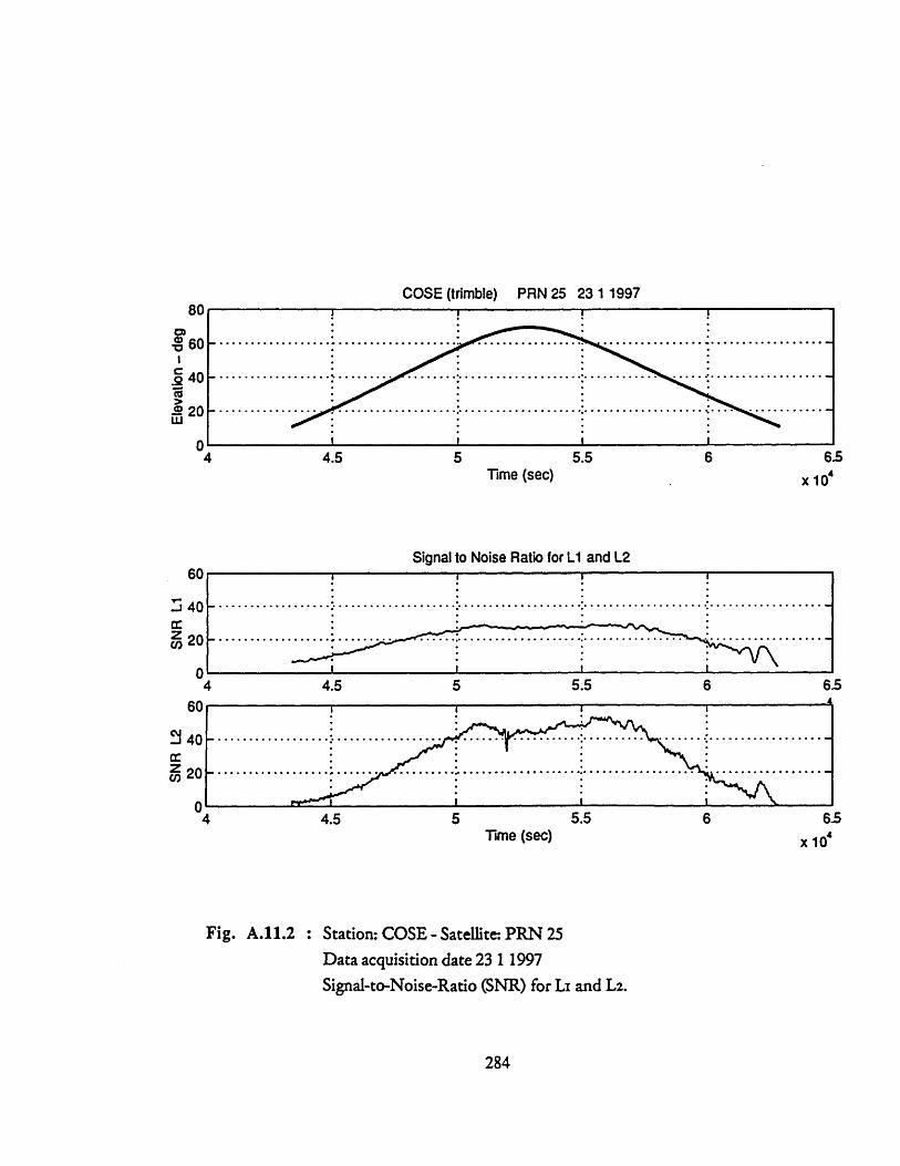
COSE (trimble) PRN 25 23 1 1997
4.5
4.5
4.5
5.5Time (sec)
Signal to Noise Ratio for L1 and L2
5.5
Time (sec)5.5
x 10
Fig. A.11.2 : Station: COSE - Satellite: PRN 25Data acquisition date 23 1 1997Signal-to-Noise-Ratio (SNR) for LI and L2.
284
80
.60
I9 40
- 20w
04
-- -------· · · ·- 1/--**--.******* · · · ·********----· ------- --------; · ·-- - -- - * ** * -* - - -- * ** *
6.5
xlo'
S - - -I I------------ * iiiiiiii
4
2C
C
6C
40
20
0
-. ........- ................ .......... .........II I I I.. .
ii i ii i ii ii i i
4
6.5
w,.r
i B I n
I
I

GPS "OBSERVED" Phase Residuals for: COSE (trimble) PRN 25 - SOUTHERN CALIFORNIA 23 1 1997
0.2 ;...................:...................................................................
0 4t.:.3 ;t"*."%. .. . j' p·,:.iS 4 \.oT:....-. .. ... . .. ........ ...... ......... .......... .......... ...... , .. -
-0.1 .
.1........ ........... ......... * .......................... ... . .-0.2 , I I I T I * I
S0CO
- -0.5
4.4 4.6 4.8 5 5.2 5.4 5.6 5.8 6.· · A LC· _L
GPS "ESTIMATED
"
Phase Residuals computed from the analys E
6.2
4.4 4.6 4.8 5 5.2 5.4 5.6 5.8Comparison LC OBSERVED vs LC ESTIMATED
4.4 4.6 4.8 5 5.2 5.4Time (sec)
6 6.2x 10'
5.6 5.8 6 6.2x 10
Fig. A.11.3: Station: COSE - Satellite: PRN 25- Data acquisition date 23 1 1997The observed phase residual (LC..OBS) is compared with themultipath phase error estimated from the SNR (LC_.EST)Unit: [cycles]
285
n .............................. * ......... ....... . ..... .. .. ........
. .. .. .......... ..... .... ........ .. . ........... . .......... .II I I I I !
-0.5
............................. .................... ... .. .. ..... .
• • • - -- - - -° -- --I i ! i! . i• * • • •····r·····~·····
I , I I I I I II
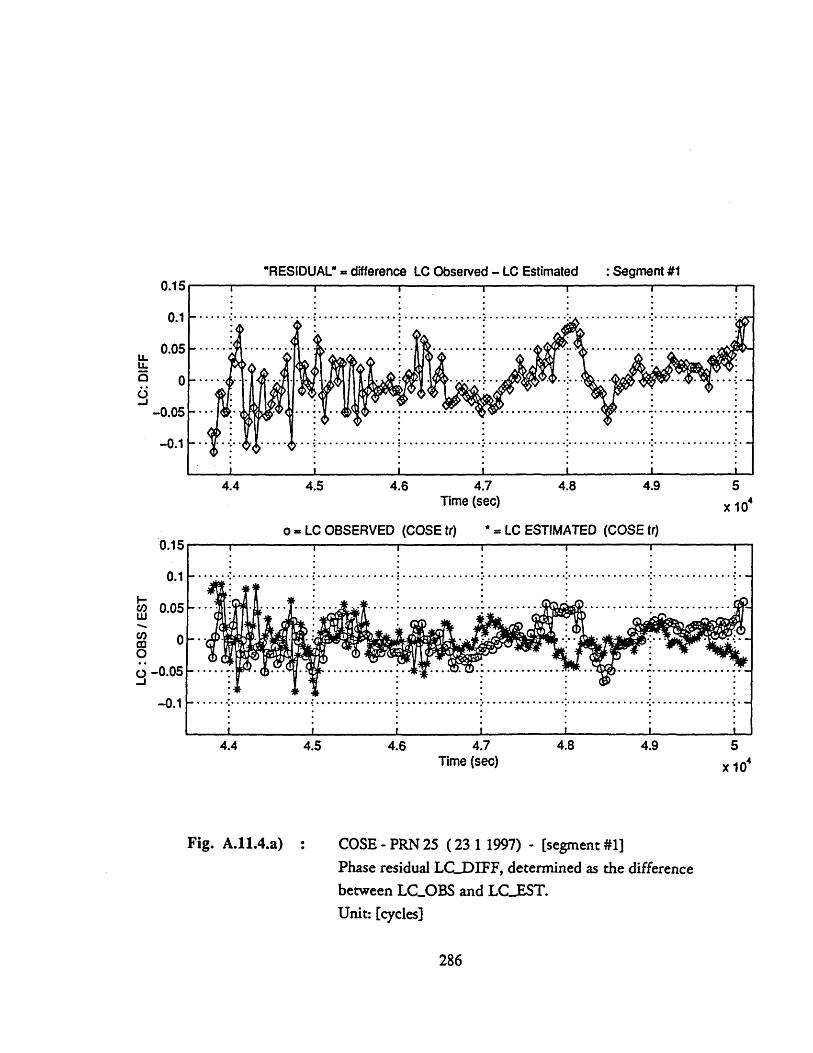
"RESIDUAL" = difference LC Observed - LC Estimated
4.4 4.5 4.6 4.7 4.8 4.9 5Time (sec) x 10
o = LC OBSERVED (COSE tr)
4.6 4.7Time (sec)
* = LC ESTIMATED (COSE tr)
4.8 4.9
Fig. A.11.4.a) COSE - PRN 25 ( 23 1 1997) - [segment #1]Phase residual LCDIFF, determined as the differencebetween LC.OBS and LC.EST.Unit: (cycles]
286
U.1
0.1
0.05
-0.05
-0.1
I I I I I I I
I i I I I
xlo'
: Segment #1
•ldL"

oo°
.| •.
oo:°..... ....
i 7
.............
.........%
,,•0• .
.....o. .
.•
.. ...... .. .
.... .....
% .. ..
0.
.. .,...
.,
..
.......... ..........:
.... .
:...... :.....
.."..
...... .....
••
• • • e.
• i
• ..
,,.. • .i
.,,,I •::i:r
•
iiiiii' :,..o
• .......
o..;
"" !
J"l/"
0 010
Sd
S0
o3
1JO
S
d
.=~Z
' =
...~·
:*r
C·4O
r~·
;4·t
..~..+. ~. r.
ct'
'3E·.
~.c.
rz.
.·j~ry~. r
-···`L
C)O
i) C
-"
dR
oI
0IC000o
...
.... .. .• .
.o. .
... .
...... .,
• .o. ..
***
.'....
....
.:..... .... ..-.
. .. .
.... •..
%............
.....
C
.....
··-°°e
°°"····
::·::: :: :::
: :: :
°.
!°
•.,•
.°
•
·° •·
i
i
i··
o co
I13 O
10
OSd
It)O O
CdI
I-C)
N01%
ao CD
o Co
C)
=1-I0 31 10 O
Sd
LO oI
SG80 31
:::::.::::.::::::..::.. .....
..,
..... .
.., .
.. ...
... .:
.....
:. ....
.... ;.....-......- .
...
... ......
.... ..
...
......
..
..
...
%
...... ..
.. .
rI
IS3 0
"z-w
ia o7
u
C4U
o
P"
u u
c~
ul1-4 ~
0 ~
u 04
gh
...
* *
•
.o
.o
@
@
@
@
••
I
I I
•
P
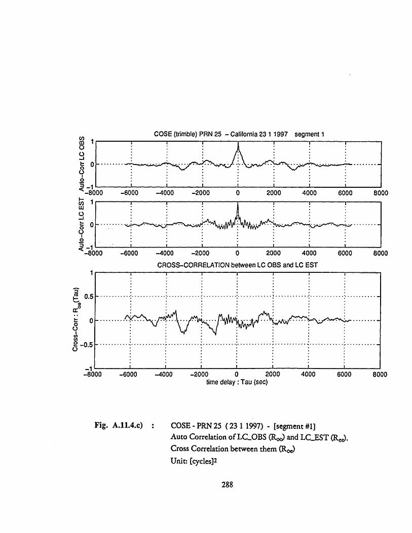
COSE (trimble) PRN 25 - California 23 1 1997 segment 1
-6000 -4000 -2000 2000 4000 6000
-6000 -4000 -2000 0 2000 4000 6000
CROSS-CORRELATION between LC OBS and LC EST
-6000 -4000
Fig. A.11.4.c)
-2000time delay :Tau (sec)
2000 4000 6000
COSE - PRN 25 (23 1 1997) - [segment #1]Auto Correlation of LC_..OBS (Ro) and LC..EST (Ree).Cross Correlation between them (Roe)Unit: [cycles] 2
288
C,,
0
0
0
-8000ino-.J
oo_jIt=
-8000
1
°°°.°°• ° ° .. I
8000
8000
0.5
0
-0.5
.4
............ ..... ............ ........... .......................
.... .... .... .. .. .. .. °. . . . . . . . . . . .. . . ..
................................ .....
1~~ I I
-8000
-80008000
...... n I
1I li b I I I B m m I I I I
I
'''''' .°. .... . ....
E

>1
0U)
CL
U)
00I-0.
C,)
0
o
0
0
0O
o
0CV
l 0
(1) S Pu
e (1) s
"1-
OCl
o O
06o
I0I
...-... ... ................
......
.....,.......
.....................
...............
..
,,,.,,,,.°o.•e,,.o,,•o·o··o·o·,··°·
•
....
......
Il· t li ilt.li
ll ll li ll·l
Ilii1111111t
··
t111
ilI
I1{*•!111
......···f···
i ...... .... /
I
IT"
oc)
LO
x
WO
E-J
Cc
C,z occ
U)
V00B
mO0z-)wccF0t U0
C)
C)
C)
CO
0
0
(W) S lO aO
flllldV
nV
c o-
o co
"6
0 06o
eouOJLqooIS3
/1o
80
31
0
C)
C)
0a.
>- J
c CC)C
.)cc
0 aTu;-
U)I-
-·l!U
)0
.. ..........
......
.....:::::::::::::':::::
·:::::::::::. ii
............ .* ... .. ......
.........
......
......
...
.t
i i
t itl ! i ii I •1i
i t
i• t i t ii ti! ! i i i
.....
: ....... ·.......
...... .......
..........
i...~s......
%.
........ ... .
% ....... ....
.o....................
...
..
uC0)
cI.L1
'
c
t4-4
0
C.0
124 O
U
0 U')
0 P
)u
-e
....... .....
..... .
.. .. .. ..
:.:.:.:.:::::::.:::::: :. .
....
.......
..... ..
......... ... ..*................
..
..
°.. .
, ,
...
•
..
.. ....
......*....................:...
.
........... ......
....
....•
....
i11
1
..
..
.1
% .
..·11
1
*1*.
i..
..
.
wU)
CL
a-ELON
cuJzcca-a.EwC
,rn
L~
'
1Fa
-0'-o
I-2
_J IO
-

"RESIDUAL" = difference LC Observed - LC Estimated
5.1 5.3Time (sec)
5.5
x 10o = LC OBSERVED (COSE tr) * = LC ESTIMATED (COSE tr)
5 5.1 5.2 5.3 5.4 5.5 5.6Time (sec) x 10
Fig. A.11.5.a) COSE - PRN 25 ( 23 1 1997) - [segment #2]Phase residual LC.DIFF, determined as the differencebetween LC.OBS and LCEST.Unit: [cycles]
290
-0.1
5
I I I I I
............. . ........... ........... . .
.". .............. .... .. ... .. ... .. .. ... .. ... .. .. ... .. .. ... .. ... .. .. .. --- --
•oo ...... o-*o ·.-oo ·. 1.o o.··.··.····.oo-oo. oo oo , .o o- o .- o
: Segment #2

.... "... .... .... .
...
...
..
..
..
..
..
..
..
..
.
.. :... ....... .........
.. ........
...... -
....
•
S
..| ee;•eee•;e
••••
..: .... .....
....
! ....
....
•:
•
•::~::::-
N
U)
-U
)S-:
0d
S8G 0 10 GSd
I I
... ... ...
... L
~L:
•.•.: .......... ·
L
%1
•r-·.,
S '7
J, ·
c•": '"'"
'1 j
N
r- O
r-
NI
I
o
... ..
o,
,
oo.. ..
o.
...
,
.....
,..,
.. .
%
..
..... ......
.... ., .. ".
...... .,
.... .
...............
c......•.r...
~.; ..
..
•
•···
•'.':.;.
'.... ....... .
IT
v- 0
1S3 01JO
GS
d
c -
0 C --I
IS
GO
011811000
'ItCco
Xi
uiIrq
uiCM
if;
In
4 U
L)
'- U
Ln
O
-l-110 01lo O
SdI Io
C;I
c C
;I
I
...
.o............
::::::::::::::::::::::....
•.............. ....
...
•, .
.. ...
.... ..
.
.. .... .. .
...... •. ....
::...... .
..
.. .
.. .:.
..... ....... .
...
, ...
,. •.o
. ,
, ,.
,,....,,8.......
.. ~.:. ...... :....
". .
ý-q-A
,0•zd04
C)
°,.
ou
Lj)E1=
In
UL~
E
i
I I
.
880 0
1_-l-lO
0-
Iji
.,.....
.,.....
I I *

COSE (trimble) PRN 25 - California 23 1 1997
-8000
AAAAP A tA ~ IhAPnn~n ~ fi En
-UUU -UUU -UUU -EUUU -4UU -UUUU v UU UVuV OVVU
CROSS-CORRELATION between LC OBS and LC EST
-8000 -6000 -4000 -2000 0 2000 4000 6000time delay :Tau (sec)
Fig. A.11.5.c) COSE - PRN 25 ( 23 1 1997) - [segment #2]Auto Correlation of LC.OBS (Roo) and LC.EST (RE.Cross Correlation between them (Ro)Unit: [cycles] 2
292
m10
o,-100
! ~-6000 -4000 -2000 0 2000 4000 6000 8000
8000
cc
0rre0,U,0-)
8000
segment 2f
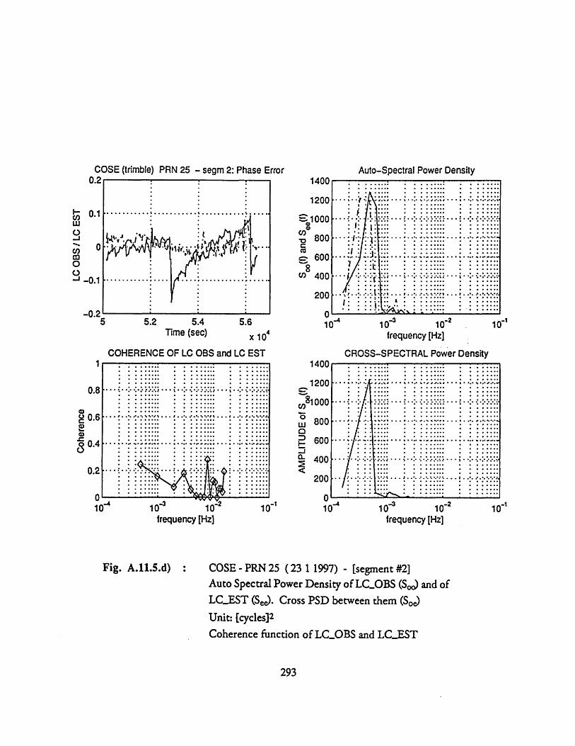
Coh
eren
ce
0 0 :9
. 0
)
AMPL
ITU
DE
of S
(f
)r
o o
o ro
41
OC
C
aaC
CC
LC O
BS /
LC E
STI c
CD cli
(D 0 -n 0. -A
'-I-
ft o a' 0 0
-A
C)S
-4
C
C·
m j55 N0
A)
ci n uto n F
, 0 0 P 0 0 '-I o CO
0 0-,
0
0r) 0 C,
ci, m 0 -4 :13
-0 0] 0r 0i u)
&C
Soo(
f) an
d Se
e(f)
0 0
0 0
00
0 0
0 0
o o
ooo
o oo
o o
..
......
.. ...
......
....
...
***.
..**.
......
...
.. ..
....
• ..
, *
......
...
..
.....
...
.. .
..
.
....
....
...
.... . .... ... ......
.............
....
........
...
.,.l.,....,,
.'·
'
.'"
" ·
: ''.
·'.
o
....
...
.
....
....
.. .
.....
....
....
....
..
...
....
*
....
....
....
...
.............
.... ..............
....
....
..
....
....
:. .
-....
.
....''°° ..
....
•'
°•I
...
.·'
: '..
......
.··
··
;·
··
·:·
·
··
.C··
1·(
·
·r·
·
··
··
·
.,··
,···
·~
·,····
__
__o
....
....
....
...
·····
· '·''.
····~
·.....
.....·
' ··
····
····
···
·~··
....
....
....
.···
............
......·
....
....
....
....
... ~··.
··
···~·
· ..............
·
...
;...
..·.
....
~...
....
......... . .. .... .. .o
.... .
....
......
.
;)V
I

"RESIDUAL" = difference LC Observed - LC Estimated
5.7 5.8Time (sec)
o = LC OBSERVED - COSE (trimble) 25 seg3
5.7
* = LC ESTIMATED - COSE (trimble) 25 seg3
5.8 5.9 6 6.1Time (sec)
Fig. A.11.6.a) COSE - PRN 25 ( 23 1 1997) - [segment #3]Phase residual LCDIFF, determined as the differencebetween LC..OBS and LC.EST.Unit: [cycles]
294
I I II i
II. . .
5.6x 10⁴
0.5
-0.55.6
I I I i
6.2
x 10
: seg #3
05I I
i

o..•°°oo~.$.o..I°..oo4(
.............
.....
.,.....
..
.I.':"
·'
S... ...-.....
-......
.~*1..=......"...
..:....
.
........
..;,.
...
.-.....-...... .....
.r
8CV
C
07 0
a
Sao
0110Jo
Sd
,,:,: ...5.
r.
• %
.I.'ii ..
.. .
•
66 46
Sao
01
0CD
::::::::::::r:::::;.
.o...
..
...
..-....
... ..
..
...
...
... .
., °
...e .
...
::~::::::::::::: :: :
...... ., ..
....
..
..
S.
...
.S.....
·r··.1
··
Cf)
C')
T-
a
IS3 01J10 S
d
CDC6
coIL)
c o
0
. cL
e)
C;
')
.....
·... .....
·%
·······(··
..... .... ..
...
.. ..
.... .
.
.....
.....%
... .. .. ..
SI
_:Ila 01 O
aSd
7777]j
4Nc'6
co0oC
D
I I
JAM-10 01
-4
-Q.
o
OCo
C)
A
Is3 01
I-
il
i

COSE (trimble) PRN 25 - California 23 1 1997 segment 3
6000
-4000 -2000 0 2000 4000
CROSS-CORRELATION between LC OBS and LC EST
6000
6000-6000 -4000 -2000 0 2000 4000time delay :Tau (sec)
Fig. A.11.6.c) : COSE - PRN 25 (23 1 1997) - [segment #3]Auto Correlation of LC.OBS (Roo) and LCEST (R).Cross Correlation between them (Roe)
Unit: [cycles] 2
296
cn0O
Co,0
0
0
-6000oI-c/)
0o-I
-6000
-4000 -2000 0 2000 4000
02C.)o(j}o
o

Coh
eren
ceo
o o
PPP
b
AM
PLIT
UD
E of
S
(f)
S o
u rC
) i
01
0
C1
o C
1
LC O
BS /
LC
EST
0-I
.010
....
....
....
. ......
....
. .......
.•,o.
...
°°
o.. :
....
.o°....
. .... "
......
'.....
." ....
. i .
. ...........
.. ...
...
.......
..
...
• .. ,, ...........
....
°
..
•
..°°
•o°•...
... ..
....
•.
.....
....
.. .. ....
..
... ..
....
;.
.....
....... :.
....
..S:
.:
: :
.....
; ...
......
...
0II
Soo(
f) an
d S
(f)
r 0
01
o C>
C0
o 0
o 0
0
-Lo
-L
C N
C)
cl 0 0 0 C,
o
01
CD ci)
)(
0
0 -AQ
C)
0 C-,
(A CA
)0 0t Q
-
oC
0
o CA C
On
Or
0.
i :0
0
..
.°
..
..
•
....°
.
... ... .
...
...
.. ...
..•....,..
.• •
• .
..
......
..
.
•······C
·~
··
··
·•·
° .
--
-° ....
,.......0.
-o.
,o °.............%...,.......%.....
...o.
. .... 0
J ..... : ...... a
:.........
..
|.i
~~L·····
··· ·
·.·
··
··
.·
..
.........
..
··~
··............
...
.... ............ .......
.......
...
... ... ....
o
.......
. ....
........ ..........
. .....
......
.....
........ :...
.. ..
....
..
....
....
...
·. ·
·.·..
. .
......
.. .
......
...
o·······o
···...
.. i.;.;..,
··.
··-.·. ·
o·····,......·...o·..
a
·I
;T%I
vdw
V0
om a I CD
() a
CI) 0o
Io C

12
15 .....
90 90
21 *. 30
240 00270
GPS DATA: receiver location: SOUTHERN CALIFORNIA acquisition date: 24 1 1997
station: GS29 (Ashtech) satellite: PRN 01 station: GS29 (Ashtech) satellite: PRN 01
3 4 5Time (sec) x 10
200
o 150I
100
Time (sec)
Fig. A.12.1 : Satellite visibility chart for PRN 01 (skymap).Elevation and azimuth of PRN 01with respect tothe station GS29
298
1
..° ..... ...... ............. .............
: *...... ...... ...... ...... .............--
Xl40
i^^
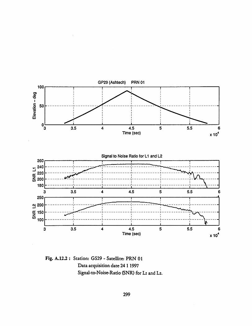
GP29 (Ashtech) PRN 01100 i
0)
* 5 0 . . . .
03 3.5 4 4.5 5 5.5 6
Time (sec) x 10
Signal to Noise Ratio for L1 and L2Zt)U
. 240-jc 220
Z 200180
ZOU
S200a: 150z
S100
3 3.5 4 4.5 5 5.5 6Time (sec) x 10'
Fig. A.12.2 : Station: GS29 - Satellite: PRN 01Data acquisition date 24 1 1997Signal-to-Noise-Ratio (SNR) for LI and L2.
299
.: ".---.-- --- .- -.....- -- ....... : ............ .. ..........
-............... ...... ... ........ . ... .... ................ .. ... .......---- I -I----'* I-- : - - ------ I---
- -------- --- i- - - - - - - * * - - - - - -- - -- - * * * - - - - - - - - - - - - -
3 3.5 4 4.5 5 5.5 6I
........ ....... ......
I

GPS "OBSERVED" Phase Residuals for: GS29 (ash) PRN 01 - CALIFORNIA 24 1 1997I I I I I
-----· ----- -----·--- -:- · · · · · _-- - -i---· · ·;····
---**** ~ ~ ~ ~ ~ ~ ~ ~ ~ ~ ~ ~ ~ ~ ~ ~ J. --- -- -- -- - --- - - --- - - -- --- - - - - - -- --y - --... .. ......................... ........ .. ............. . .... ..-. . . . . . . . ... . . .. ..-- . . .--.- rt ----.. ... "" "
.. ................... -................... .................... ................... . .........-
................... I ................... .................... .................... I ..... ....4 4.5 5 5.5
GPS "ESTIMATED" Phase Residuals computed from the analysis of SNR variation x 104
3.5 4 4.5 5 5.5
C i LC OBSERVED vs LC ESTIMATED:
art 1
0.2
0
-0.2
-0.4
-0.6
0.4
0.2
0
-0.2
-0.4
-0.6
5.54.5Time (sec) x 10
Fig. A.12.3 : Station: GS29 - Satellite: PRN 01Data acquisition date 24 1 1997The observed phase residual (LCOBS) is compared with themultipath phase error estimated from the SNR (LC_ES'I)Unit: [cycles]
300
0.4
omparson p
• .. .. ....o.oo .o ,..... ...... o .... ..... .o ...° o oo o o o o o.. ..... ........oo o o....
............. ............ ....................l .................... . . . ... . . . . . . . . . . . . . . . . . . . . . . . . . . . . . . . . . . . . . . . ......... ...... .... . .
....................................... . . . . . . . . . . . . . . . . .--··· ~ · ·~·~~~~~ ~~~'''''- **' '''''''''' ----------- ----- - - '
0.4
0.2
0
-0.2
-0.4
-0.6
I l.. . .
.. .. .. .. .. ...° °... ..... °.. . ... .... . . . . . . . . . . .. . . . . . . . .
.. I ................... ......... ......... ..................................... .......................... .................. -- ----******** ------------ ---- *************** ****************·· ***------
j- ** ** ** ** ** * -- * ** * * ** * * ** * * * * * *

GS29 (Ashtech) PRN 01 - SOUTHERN CALIFORNIA 24 1 1997
3.5 4 4.5 5 5.5Time (sec) x 10
3.5 4.5Time (sec)
5.5x 10⁴
Fig. A.12.4 : Station: GS29 - Satellite: PRN 01Data acquisition date 24 1 1997LC.OBS and LC.EST compared for t=3.5 - 5.7 10 4 secUnit: (cycles]
301
U,•
0.2
0
-0.2
-0.4
-0.6
. .. . .. . . . o. o. ... . ,......o...... . o.... ..... .
- - -- :-- - - - - - - - - : -- - - - - - - - - :-- - - - -- - - - - :-- - - - - - - - :. .i I I I I'=""" """" ="""" """" .ii
I''''' · ' · · I·s' · · · · · · I··· · · · · · · · · · · · · · ·
,,

"RESIDUAL" = difference LC Observed - LC Estimated
3.3 3.4 3.5 3.6 3.7 3.8 3.9 4Time (sec) x 10
o - LC OBSERVED (GS29 01 Ash Part la) * = LC ESTIMATED (GS29 01 Ash Part la)
3.4 3.5 3.6 3.7 3.8 3.9 4Time (sec) x 104
Fig. A.12.5.a) : GS29 - PRN 01 ( 24 1 1997) - [segment la]Phase residual LC..DIFF, determined as the differencebetween LC.OBS and LC..EST.Unit: [cycles]
302
0.2
0.1
MO 0
o -0.1
-0.2
3.3
: Part la
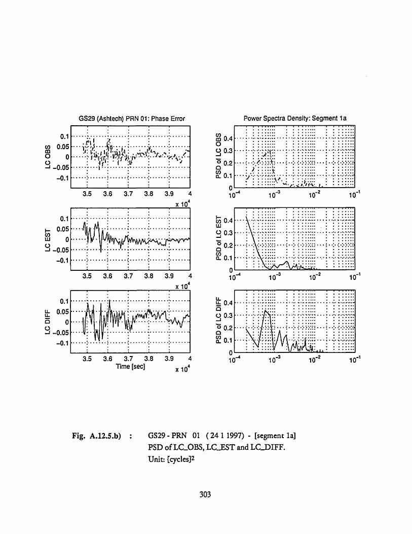
....
|*....
,oo.. .........
........
e*...*........
°°°•°° • c.....
: ........
...
..
....... .............
...... .... ...
••....r...r.. .
....
:::•::
°. ......
.~ :.'' .,.. ?
.°....
" •s'•
o.r
··
··
I ··
t· ·
~:···I·°
0lo1"
Cor
SO
0
1- 0
,-
S80 0"I 10 O
Sd
IS3
0 0
0S
d
... ...
....
.......
• ...-.... .....
:.... -...
... .-. .. ..
...
... ..
.. ....
..............
:... .
..... ......
i: °1
.. :..
.•.
..
r•.° .°.
••
•...
....
:..°° *..•°...=.°
CV
" C
1 C
- 0
-
JJIII 0
"1
0 O
Sd
N.-
I "
I83
07IS
3 01
0 dII
::::::;:::::::::;:::•...
...• ....
:... .. •...
• •... •
.....
..•
.
•''(*°-•*°°••°°°*•
•.. •. •~ r .
... :.... ?
Cv)
EcoU
im
•
"T
tV--
V-4
Ntcq
gP
g

8
I00.4
GS29 PRN 018 Califomia 24 11997 segment la
[I~ . . ..... ~
-5000 -4000 -3000 -2000 -1000-5000 -4000 -3000 -2000 -1000
-5000 -4000 -3000 -2000 -1000-5000O -4000 -3000 -2000 -1000
0 1000 2000 3000 4000
0 1000 2000 3000 4000
CROSS-CORRELATION between LC OBS and LC ESTI I I I I I I I
I I I I I I
-4000 -3000 -2000 -1000 0 1000 2000 3000time delay : Tau (sec)
4000 5000
Fig. A.12.5.c) GS29 - PRN 01 (24 1 1997) - [segment la]Auto Correlation of LC..OBS (Roo) and LCEST (R).
Cross Correlation between them (Roe)
Unit: [cycles] 2
304
cc
I0<a:
I I .I
. .. .. ....
I ! ! I ! I ! I
5000
5000
0.5
oa00
-0.5
_1-5000
T m I B I I
__ I4
J

(D
a.XU
)C0)0C
)
oaC.)
v)0.
C,,
o o
0 0
0CD
C)
C)pe~~,ee
C)
C)
w
w
IV
m:
00M(I)o SPU
E (I)
s
r- )
d q00
oo
IS3 01 / SGO O1
oi, ',,
,,,,.• ,
.... ........
%
.. .o.o e
.... ... -
.. : .
.,. .
... .
... .
..... •....····5·
·.·...~.·.. ..........··
...
•. ... .
...
... .. ..
.. •. .... ...
... .... .
.o
.% ...
..
...
,
,
..
·,
.o .o o o , , ,
..... ...
...
..
.....
.. ..... ....;.-... ..
....-
!,: !i !,:,: !i! • .• ....
: • • ! •?:!····.,.
!.
·.] ! ] ] ] :.
[]
!]i
] ]i,"
[ ,
: "
,zi
11-o
0 0
0 00
0o
o 0
0 0
0 C(,-
CO
OT
'T
nl• V
(1) S Jo 3flhIdidN
V
x0)coEi
(ot)E
c oD
co
l C
4
~12
0,.COI C
)
00a: 1F-0C
,)
C,)
0a:0
CCC
:: :
: :::::::::: :::::
·:::::
......
... .
.. ..
.... ......
....
.......... .
.............. ........
..
.. ...
... ..
......
.......
........;
......
.... .
..... .
I .
.. ..
.... ...
.[.,.
.......
..
%
,,,,,,~
....
,,.,~,.....4.·.
··
··
···
.·..·,··
··
·(,....,
'''''' '
''' '
1"0.,-
0
cec
as•00
uQoO4,)
0rO.
C/)
:30
-Cý
I-b0
V)0uiCi
Ht
******.*
*****···
******:-****.*****..
..
:*.
....
...
......
0...............
.. ....
............. .......
.o....
...
........
..
:
.... ............
:
.....
:::::: ::::::
::::::::::::.. "':
******;****** .**.*.;.*...**.*.*.*.
........ . .k
LT
~-~··.........
........
...
c~4
u
IcrC?
0*cC
e
0
• •
..
• ,
--·
·
•
•
•
i
o
.....• ...
..: ...... :......S'
.....;..
.'. ,.
•..;..... :......
...
..........·
·~ ~
~~
C
·r ·
··
·=
h •
, .
(o8

"RESIDUAL" = difference LC Observed - LC Estimated
4.1 4.2 4.3 4.4 4.5 4.6 4.7 4.8 4.9 5Time (sec) x 10
o - LC OBSERVED (GS29 01 Ash Part Ib) *= LC ESTIMATED (GS29 01 Ash Part Ib)
4 4.1 4.2 4.3 4.4 4.5 4.6 4.7 4.8 4.9 5Time (sec) x 10"
Fig. A.12.6.a) : GS29 - PRN 01 ( 24 1 1997) - [segment lb]
Phase residual LCDIFF, determined as the difference
between LCOBS and LCEST.
Unit: [cycles]
306
0.1
0.05
-0.05
A I-.4
: Part lb
t-W

LC D
IFF
C
PSD
of L
C D
IFF
0 o ...
. ..
...
....
......
......
......
.. .....
......
..
.......
.....
..
..
.
C
...
...
...
......
I ·
·c
··
r·
··
··
·
LC E
STI
0P
*c
n-&
C
ila
PSD
of
LC E
ST
k
....
....
..•
o...
. .............
...
....
. ..... .
....
.. .
o..oot o
.o ...
...
.O .
oo. oo.o. .oo.0.0.o.O
....
....
.. .
..
.•..
...~
...
....
r..
...
•.....z.
..
:::i
::::
:!::
:::•
::.'
.·1
· ·
·~*
LC O
BS
I O
o
0C0
-& (
3 0
(1b
-
.i.
C>
(n
S.
o..... ....
bo (31
PSD
of L
COCB
So
0:'
.. ...3
..
•
.1 o•
•
.a -.
.... ~
~ ·.
•
·.
:...
: ..
-: :
PSD of LC OBS
O
O
O
'1.....
:
...
.• ~
~
~ C
•
uo
..
.o o o
o.··
t ·
··
··
·...
..•.-- , ., ..
.. ..-
.....
-.......
.•·
··
··
·;·
·
•
••
o
o ooo
·
0........0~..***...
.....
•.....
.:.
....
• .o**;0 • ojii~.. .
• •0o0
::::
:i::
::::
,:::
::•:
3 CD
c,) 'ia
) bo
S(n
1

GS29 PRN 018 Califomia 2411997 segment lb
. . .. . . . . .. .
-8000 -6000 -4000 -2000 0 2000 4000 6000 8000
-8000 -6000 -4000 -2000 0 2000 4000 6000 8000
CROSS-CORRELATION between LC OBS and LC EST
-8000 -6000 -4000 -2000
Fig. A.12.6.c)
0 2000 4000 6000 8000time delay :Tau (sec)
GS29 - PRN 01 (24 1 1997) - [segment Ib]Auto Correlation of LCOBS (Roo) and LC..EST cR).Cross Correlation between them (Ro)
Unit: [cycles]2
308
c80csI0
0
oI0.
. . ...I I I I
IIII I
0.5
0
-0.5
0to
U,0U..UO
I I I I I I I I I

00-a-U)
0.U
)33
o o
Co
o
oC
(W)O
o 0 3an
-ldV
000
UO
2C
o 0 0
o .0...
c'C
?
D
(0D
q cd
0
0
0
0
tFJutJ
iLru
)j
IS3 01 / Sao 01
A::U,C0a<C
CCL
!Ow
U)I [U
)(0cc0)
oTI-
I
-0
Sop(0 0
=4)
4rd
4.
/'I
_-·
>
o
C)
a-E0)IC)zcca-C.)
0a)
0m
coU
)(9
...............
*. ..
: ::
: :
..... .................. ...........
.................. ...........
:::: ::: :::
:::: ::::
: :
:: :
: .
............. *.............*.........................
:.~..~....,........!
...............
% ...............
...........
........,...... .......
........... .
--
-..........
.**.* .*
....
**.
.. *.
* ... .
**.*..
****.*.. *. *
."
' *
* t
......
....
.....
V-U
)x
W
0 O
SOm·
i o0cun
0)Et L00zO
c wO
S
cc.~.
wM0
r
Hill
iX
-- --
cl
cl o
c--

"RESIDUAL" = difference LC Observed - LC Estimated
5.1 m 5.25. 5.45. 5. 5. .
5.1 5.2 5.3 5.4 5.5 5.6 5.7 5.8Time (sec) x 10
o = LC OBSERVED (GS29 01 Ash Part Ic) * = LC ESTIMATED (GS29 01 Ash Part Ic)
5.2 5.4 5.5 5.6 5.7Time (sec)
5.8
x 10'
Fig. A.12.7.a) : GS29 - PRN 01 (24 1 1997) - [segment ic]Phase residual LC.DIFF, determined as the differencebetween LCOBS and LCEST.Unit: [cycles]
310
4
2
0
2
4
6
85
-0.
-0.4
-O.E
-0.
0.e
0.9
-0.4
-O.E
........... I ~ ~ ~ ~ ............ I.... ................ I ............... ...... .. ... ...... ...... ......
..................,
.... ... ... ... ... .... ... ... .. .. .. .. . . .
. . . . . . . .. .. .. .. .. . .. . . . . .. .. .. .. .. . . . . . . . .. .. .. .. .. . . . . . .
. . . . . . . . .. . . . . . . . . . . . . . . . . . . . . . . . . . . . . . . . . . . . . . . . . . . . . . . . . . . . . . . . . . . . .
2 ....... ....... ...... ....... ......
g I i2 - -- -- · - :------------· · · · · · · :· -----------· · · ·
4 · · ·- · · · · ·-· · · · · · · · · ·
5i I i i i
SPart lc)r-
0.,

.....
5. ..... ·
....
..........
,
..o......•........'.....
....
o.. ........
.... ...
.. .: .... .
.1.
...
... ...........
.....................
i~
S .. ...
....
.
..........
..
.....
.. /
.... .. .=...
1•• •: .. ..
co cD
It
C
C
0
-
SO 0-10 GloSd
IS3 0- IO
GSd
.....
*.
.....
* * .....*
°...
.. ....... ....o.°.
,. .
..
,.....'. ..
..
....
•............•..
..
................i
ii
cD
cD
q CJ
,-
JJO 301 o
0Sd
4.-
:.~
F............··
··
4.
I
SBO
01
U)
O
U)I 1
IS30 '
-o
0%4
0iE
C'j
0 0
ITo
·;
it

GS29 PRN 018 Califomia 24 11997
-6000 -4000 -2000 0 2000 4000 6000
-6000 -4000 -2000 0 2000 4000 6000
CROSS-CORRELATION between LC OBS and LC EST
........... . . . . . . . . . . .
.... . .. . ...
time delay : Tau (sec)
Fig. A.12.7.c) GS29 - PRN 01 ( 24 1 1997) - [segment Ic]Auto Correlation of LC.OBS (Roo) and LC=EST (Ra.Cross Correlation between them (RoUnit: [cycles] 2
312
0
00
I-
0 -0.5
-6000 -4000 -2000 2000 4000 6000I
segment 1c
.. .. . .. .

Coh
eren
ceo
o o
I.u
I b
CD
0
Ui
0)
AMPL
ITUD
E of
So(
f)S0
0
0 0C
0
C:
: : •1
LC O
BS /
LC E
STo
-C
L
JI
S (f
) and
S
(f)
nooo
c o
oCoC
o o
C)
C) C
) C
L C
oo
G
E.
'.3
C..
0 0t -I C), 0
-
C.)
H
Co DO
0 z "0 Ca
(O 3 o -3 P, f) CD
I II
0·
c-
cn
O
o8
C,,0
c:m
o o O( V)L 0
r0ij
1
.. .:i .
.. ..
:i: ..
... .
.....
......
...
. ..
....
...
.
o..........
*. .
.....
...
...
...
....%...o.......
..°..•.•.....
.
..
....
. ;
.• .
.'...
...-.
...
......
.
.....C.-.".
..
I ..... •..... I ....
•.
..
.. .... .
.. ....
• ...
..| .
..... .
.. .
.1 ..
.....o .
..
..
o.' i..**.,
·. .. ........... .....
.
.°.. ..... .
.. .
..o ....°.° °. ..
.°
... .* .° °.
....
. :.
.... ;.
.....:
.....
;..
.. .
.........
o...*°•
.* .........-. *..
..
•o
o ° .....
.°...
.....
°... .
°. .
oo
o
....
. •.
.....:
....
..:.
....
.:..
...
."...
...
....
. ...
......
......
.. ..........
.. .. ..
.....
.:
.... .
.... .....
... ..
....
....
..
X
.....
• ..
.: :-
: ....
......
......
.
..
...
........
....
. :
...
...° ... .t
... ... ..... .....
.. ......
...........
....
....
..*'*' .''' '°O '''. .o .*
°O
*.
.. °*
....
:
:...
..:.
....
. ....
...:..
..
• ..
...
o. ..........
.. ..........
I i i
i i ::
i I i
i i i
i i i
iii i
i i i
i i i i
r iri
I i i
i I
mi
......
..
......
......
.....
• ........o..•...........
....
....
. ..
....
{.......)
......
:...
...
: :::::::::
::::
:::i
:::;
:·::
:::
....
....
...
z.......
...........: :··
··..........
~...
....
...=
....
...
......
......
......
....
....
:) .

1290 90
18 . .. .:00041 .... ··....... 0
240• . 300270
GPS DATA: receiver location: SOUTHERN CALIFORNIA acquisition date: 24 1 1997
station: GS29 (Ashtech) satellite: PRN 07400
300
200
100
00 2 4 6 8 10
Time (sec) x 10
station: GS29 (Ashtech) satellite: PRN 07
0 2 4 6 8 10Time (sec) x 10o
Fig. A.13.1 : Satellite visibility chart for PRN 07 (skymap).Elevation and azimuth of PRN 07 with respect tothe station GS29
314
100
................ ·--i--- · c ~·-
· · · ·· · ·--- · · ............... · · · · ·
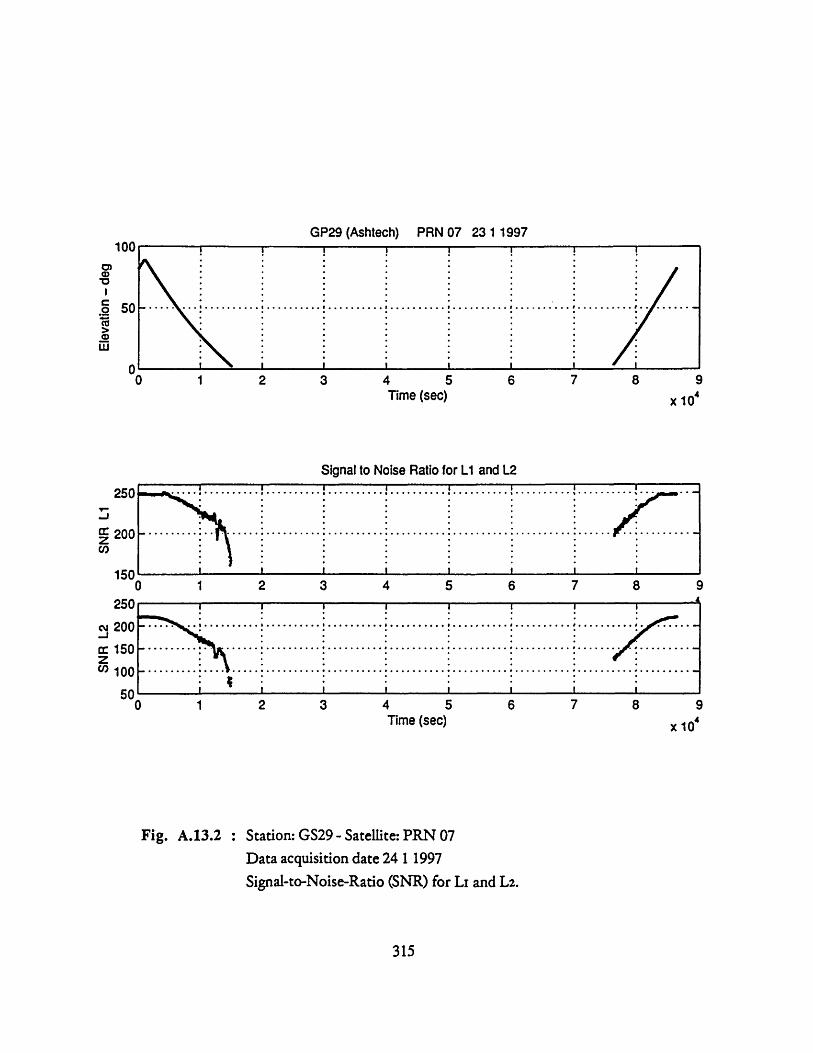
GP29 (Ashtech) PRN 07 23 1 1997
0 1 2 3 4 5 6 7 8Time (sec)
Signal to Noise Ratio for L1 and L2
Time (sec)
Fig. A.13.2 : Station: GS29 - Satellite: PRN 07Data acquisition date 24 1 1997Signal-to-Noise-Ratio (SNR) for LI and L2.
315
1
0I
.L
9
x 104
250
a: 200
150
250200
150
100
50
.- . . . ..-. ........ .......... .......... - .......... ............ ......-.--
.......... -.. -- .......-- .....- - -- -- - -.......... ......... .. ... . ..........
0 1 2 3 4 5 6 7 8
I\j.. .. °° ... .·-·... .. °,...... ... ................... ..... ..........-:* **- -- ..........-** *** ......... * --. .. ..... ..... -- --: --- --- -:- --- ---- --- --- -- : --- --- - -- --- --- --- -- -t
0 9
x 104
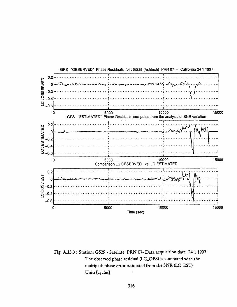
GPS "OBSERVED" Phase Residuals for :GS29 (Ashtech) PRN 07 - California 24 1 1997
- - - I -
............................... ..... .......... ........ .............
\.'.:::''''''
5000 10000GPS "ESTIMATED" Phase Residuals computed from the analysis of SNR variation
5000 10000Comparison LC OBSERVED vs LC ESTIMATED
5000 10000Time (sec)
Fig. A.13.3: Station: GS29 - Satellite: PRN 07- Data acquisition date 24 1 1997
The observed phase residual (LC.OBS) is compared with the
multipath phase error estimated from the SNR (LC_.EST)
Unit: [cycles]
316
0.2
0
-0.2
-0.4
-0.6
0.2
0
-0.2
-0.4
-0.6
0.2
0
-0.2
-0.4
-0.6
. ...... ... .... . .. ... . ... .... .. .........
. .. .. .. .. .. .. .. .. . .. . .. . .. .. .. .. .. .. .. .. . .. . . . . .. .. .. .. .. .. .. ..
. ... ... ... ... ... ... ... .. . ... ... ... ... ... ... ... ... ... ... ... ... ... ... ...
. .. .. .. .. .. .. .. .. .. .. .. .. .. .. .. .. .. .. .. .. .. .. ..
151
154
15(
000
000
000
I
.,.............................-
... .. .. .. .. .. .. .. .... .. .. .. .. .. .. .. .. .. .. .. .. .. .. .. ..... .. .. .. ... .. .. .. ... .. .. .. ... ... .. .. .. ... .. .. .. ... .. .. ..

GS29 (Ashtech) PRN 07 - California 24 1 1997I i 1
5000 10000Time (sec)
5000 10000Time (sec)
Fig. A.13.4 : Station: GS29 - Satellite: PRN 07- Data acquisition date 24 1 1997
LC.OBS and LCEST compared for t--0.0 - 1.4 10 4 sec
Unit: [cycles)
15000
15000
317
0
-0.2
-0.4
-0.6I i i I
-0.2
o -0.4-0.6-0.6
. .. . . . . .. . °.. . . ................................ . .... ............ ..................
.r I. .H '•, ....: • .,.,(,,- .',.*,,:.-,. .., ,.,,.,., . .',-,..,.+•,..-,,.,,.,.,, -.,'-: "',.":)~:2·+··~·~··· •u • ,, ,' ..•..."¥ •.. .; a.. ... .4x? |
I I.°..•........°% °... ....... °°..... -
................ ........................... ............... . ....
....--- ·....... ...... ...... ..... ...............................
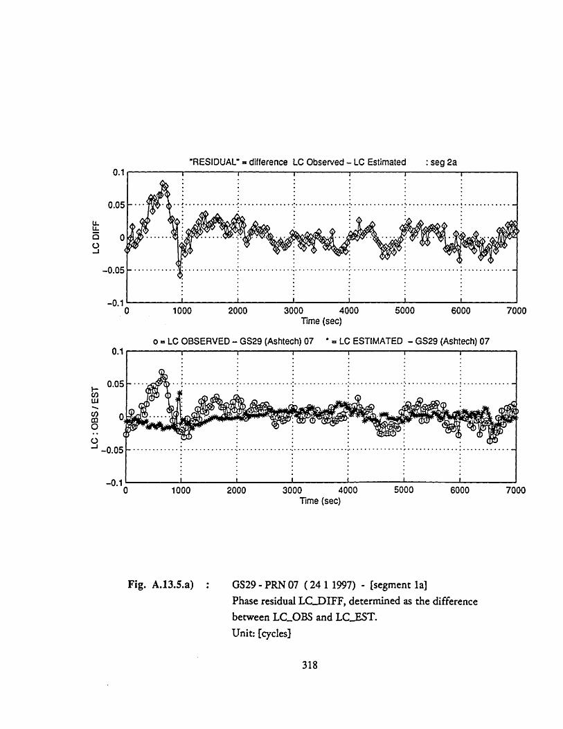
"RESIDUAL" = difference LC Observed - LC Estimated
0 1000 2000 3000 4000 5000 6000 7000Time (sec)
o = LC OBSERVED - GS29 (Ashtech) 07 * = LC ESTIMATED - GS29 (Ashtech) 07
0 1000 2000 3000 4000 5000 6000Time (sec)
Fig. A.13.5.a) GS29 - PRN 07 ( 24 1 1997) - [segment la]Phase residual LC-DIFF, determined as the differencebetween LCOBS and LCEST.Unit: [cycles]
318
v. I
7000
: seg 2a
I
I-%.

I.·?'·''''·
.1·
....
..
.. ....
.•. o.. •o
%..
..: .
o .o. °. .o...
..... e.....
......
••.
...
o
.... .....
.. ..........
Of
..
...
•• ..
... .. .
...
..
..
............
..
..
......:.... ........;..•
• •
• s ..L
: •
'. ''•.'
.... .
•,•
..
2 .....-.;•"..,•
•
• •I... • .......
.
.... •....
.....
=.
.-
.
0
0N
' )
U
I
SO
O 110oGSd
I I
..·..
..
.. ..........
.. .
....•
•
..
... ..
...
7.v
N c•-
0 -I
II
IS
80 0-1
@@@@ o@
'@o.... @......
-..... ....
....
;.....
......
....%:
....
......
...........
.o..........
.. .•...... .....
%
..
.. .
... .............
................%
..
o. .....
...
'.
..
.
..
...
...
..o
..............o...
.. .•. .
.:......?...
.
..
..........
o....
........
'0....'....~··.
..... i..... ;
... ·...-
s
Ln to
CD
C )
C >
C-;)
00
010 0
0
0
.S3 0-1 Jo O
Sd
ooCCD
co0C)0)0~
0-
N
T-
o0 -
j
I I
.LS• 01
%... ...
.... .....
..
...
........
...
....
.
.... .
... ... ......
..•
...
...
oo .
....... .
o
.. .
.o.. oo ·....
.o. ...
• ...
I
,~~.ooo
o•.-
NV
U
) '-
U)
0,
0 .
00
0
-110 01 Jo O
Sd
ooo00Cl
o0
d
V-
0 -
c
=u0a 01]
Cdo
4)
'C 4
0 ''
C3O
4
C)0
P
I
I :
I

GS29 (Ashtech) PRN 07 - California 24 1 1997(A.
-6000 -4000 -2000 2000 4000 6000
CROSS-CORRELATION between LC OBS and LC EST
-2000time delay :Tau (sec)
2000
Fig. A.13.5.c) GS29 - PRN 07 (24 1 1997) - [segment la]Auto Correlation of LCOBS (Roo) and LC..EST (Ree).Cross Correlation between them (Roe)
Unit: [cycles]2
320
m10-jt: 00
C.)
c)-Jo1...0
0ooIo
2Q*
-8000
0U
-6000 -4000 -2000 0 2000 4000 6000 8000
3(U
0
CI)0I-
0
8000
0.5
-0.5
_1
-8000
- . . . I . .
. ..... --...•"•""••"- r † . .. " '/ ".'.v . K . .; -
.I I I i . .
-6000 -4000 4000 6000 8000
segment 2a
0-Uu

0 0
o C
)0
C)
o L
n
(I)aS pue(I)O
OS
00
000(C0 -C)
o
aC
:E0C
)00c'J
CiI
1S3 01 / S
aO 01
o o
o0
o s Jo
nnfllldVV
o o
o 6
dU
dOJO
L
...
........
.....
.. ...
.......
:: : ::::::: ::::::: :: :::::
: :
• .}..........?
..........:................. .... .....
... ......
... °............................
.°
......
........ .............
o..
I
.X
...
......... .... ....... .... .
..
..5 ... .. .
...
.......... ....
..
o. ..
...; ..........
........ ........
............ .................
... .. ..
.. ... .... ..... ..
U)
Ca-t30o0III
a-CU
cliECD
a)u)
zcc:a-
r'(!c0o c
o%.4.4
aoU
SON4
4.'
....
......--
--
-:..
.. .
............. r.........
.................. .
.....
%.....
: :: ::::::::::
:::::: :
..
.......... %
...... ......
·.
.t...... ......
·2····~ ···
"t "··
··*··
52 .... .
.................... .......
..................... ............
(.4Ui
L
hi
£
*,-o
,-
c1
1,
"o
e
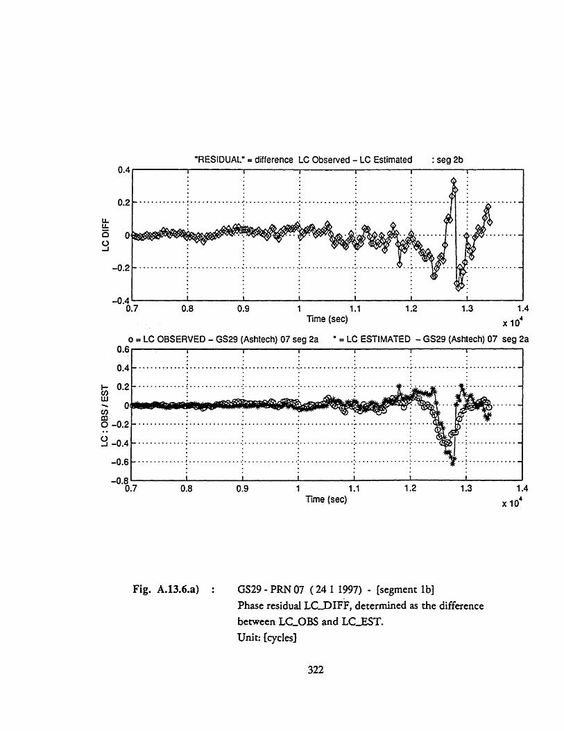
"RESIDUAL" = difference LC Observed - LC Estimated
0.9Time (sec)
1.2
x 10'
o = LC OBSERVED - GS29 (Ashtech) 07 seg 2a * = LC ESTIMATED - GS29 (Ashtech) 07 seg 2a
0.7 0.8 0.9 1 1.1 1.2 1.3Time (sec)
Fig. A.13.6.a) GS29 - PRN 07 (24 1 1997) - [segment lb]Phase residual LCDIFF, determined as the differencebetween LCOBS and LCEST.Unit: [cycles]
322
_ A
0. 7i i iI I
xl 0
· 1 I 1
I
: seg 2b
,~~..~.~~.~..~r.~.......~...~...........
..
-I
L,
0%
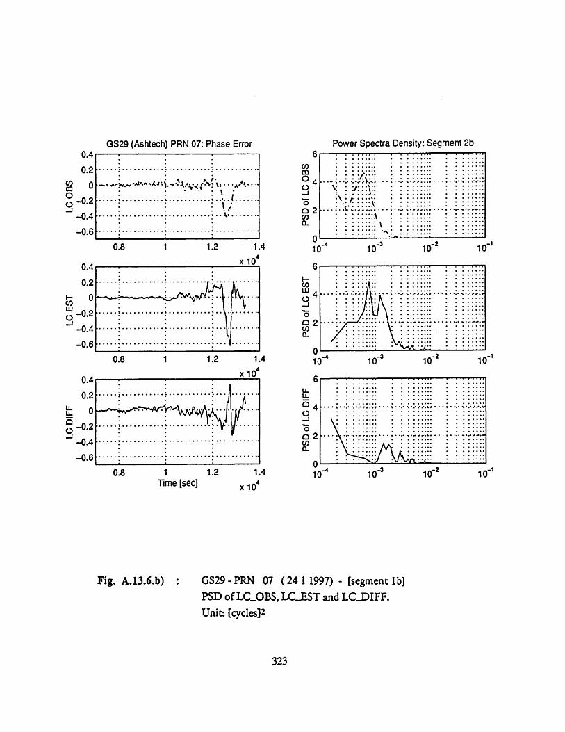
*. .
* *l.......... ..
... .
...
.............
........:.....
.....
.....
......
......
..
.. .....
.....
..2; .
... :.. ..
·l
J··
80 37
1o
0Sd
oooo• I!
° o
•I" €•I
O
•880 0
"7oI
IS3 07
=1110 07
c,r
NIor
7or
.........................................
........ *..******
.................
.. .... ....I
.............*..
*:: :
:: *
** :
:: :
:
******.............**..........................
...... • ......
*************?*
*****
......
*
* *...o ....
..
...... ::........°................o. .....°.o,•..
.o
• •
.... ...
1..
I
•JO
-Io
A,
Prr
co -
CU
oC
IS3 07 1o 0Sd
P
-191 011 oSl
14T:
I '
i i
I i
.°
..·4'··..r) ·
.o
° oo•o
• •
•
EE
P
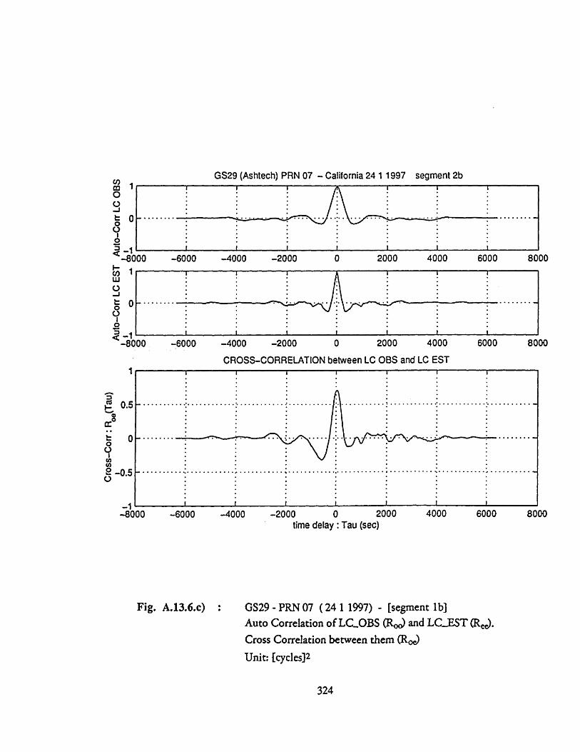
GS29 (Ashtech) PRN 07 - California 24 1 1997S .,
-4000 -2000 2000 4000
8000
6000 8000
CROSS-CORRELATION between LC OBS and LC EST
-4000 -2000time delay: Tau (sec)
2000 4000 6000 8000
Fig. A.13.6.c) GS29 - PRN 07 ( 24 1 1997) - [segment lb]Auto Correlation of LC..OBS (R.) and LCEST E).Cross Correlation between them (R)
Unit: [cycles] 2
324
0C.)-j,OotoL-I00oo,2
-8000L-
oc-)00o
-6000 -4000 -2000 0 2000 4000 6000
-8000 -6000
0o
2-C)
0.5
0
-0.5
I B B
........ ............ ,
-8000 -6000
segment 2b
. .. . . . . . . .
m.lI

o O
o
o
(1) SpuL
8 (W)OS
IS3 01 / S
0 3'1
0
C.)
C
S)cl0a'
....°.....
°
......°
....
..
°.......
..
°......................°.......
::::::: : :r:: ::: ::::::::::::::
.. ... °
.• .°...
.°.................
................"..
...... .......
.......... ................
.. ..........
...
.......... .
..
........
..
......·
....
.... ...
.. ...
....
.......
.........
......
SIoCC
a
cov,
0(1
)m
0) --
r
ZL U0wzwcc00
(C) O
JO
f>
o
o oC
S10o 3anlndY Y
Y
'- c
c c'
-o
D o0o
GougJOeLoo
c
-)n-waO
nC
oC
0
.......
.. .....
....
..-
I -.. -
......
... ........
...............
::::::::::::::::::::::::::::::::::
""""" """'
" """""
"....
...* ................ .......
:::::::* ::::::::*:::::::::::::
.... .. .
..
.... .
..
...
..
... ...
......... ..
..
..
..................
..
..···...
.. .. .. .. .
. .. ..
..
..
···
··.
.........
..
..........
0)
V-
o
'-4oIoOC
i,4
.
U)
......
:......
......
..........
...
.... .
... .
.*
..o
.... .o
....
......
........... .......
....
...
..... .
..... ......
....... ......
• •·~
···~······
I
··
i i
i
aa
v.-
Cov.

90 9012 -60
240 300270
GPS DATA: receiver location: SOUTHERN CALIFORNIA acquisition date: 24 1 1997
station: GS29 (Ashtech) satellite: PRN 25
0 2 4 6Time (sec)
400
300
200
100
0
x 104
station: GS29 (Ashtech) satellite: PRN 25
4 6Time (sec)
Fig. A.14.1 : Satellite visibility chart for PRN 25 (skymap).Elevation and azimuth of PRN 25 with respect tothe station GS29
326
x 10
=............................. ...... ............. ..... .......
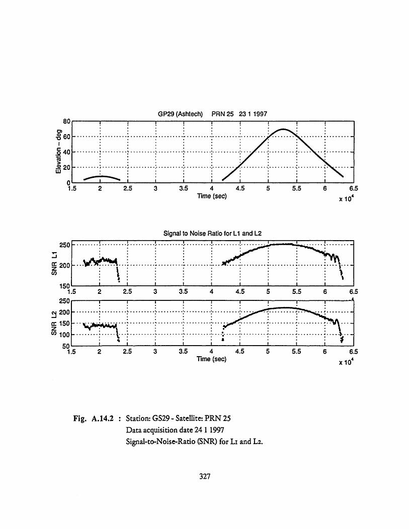
GP29 (Ashtech) PRN 25 23 1 1997
U %1.5 2 2.5 3 3.5 4 4.5 5 5.5 6 6.1
Time (sec) x 104
Signal to Noise Ratio for L1 and L2
1.5 2 2.5 3 3.5 4 4.5 5 5.5 6 6.'n _4
2 2.5 3 3.5 4Time (sec)
4.5 5 5.5 6 6.5
x 10'
Fig. A.14.2 : Station: GS29 - Satellite: PRN 25Data acquisition date 24 1 1997Signal-to-Noise-Ratio (SNR) for LI and Lz.
327
S60
I
.o 40
20
I I I
25
-j
M 20z
15
94
S200a: 150zCO 100
501.5
.... ...... ......... ...............
................. ........... ...... .......* . .8- -------- ·. · ~· ----- ~ ~ · ~.·~ . 1-----·C · · · ·· · · · · ·· ·-- -: · · I -- - - - - - - -- - -
XIM
m m m m i m m m m
,,
, ........... .. ,.......!!
..... ...........---------------- . ·---- · ·---- . -- - -- - - -- *
- - ----°° .° . --° ---- °--°- °- °-- °- °-* ° °--- ° °-- . °- ° °--*-° °,
.°.-. . . . .° . .°.,. . .°. . . .°. ... .° °. . . ... .°°. .
........ ° .. °....°.. . . .. .... ° ... °.. .... °. ........ .
;· · · · · · · · ·; ; ;··· · ···

GPS "OBSERVED" Phase Residuals for: GS29 (Ashtech) PRN 25 - Califomia 241 1997
0.20.1
0-0.1-0.2
0.2
0.10
-0.1-0.2
4.4 4.6 4.8 5 5.2 5.4 5.6 5.8 6 6.2GPS "ESTIMATED" Phase Residuals computed from the analysis of SNR variation x 10
4.4 4.6 4.8 5 5.2 5.4 5.6 5.8 6 6.2Comparison LC OBSERVED vs LC ESTIMATED x
x 104
0.20.1
0-0.1-0.2
4.4 4.6 4.8 5 5.2Time (sec
5.4 5.6 5.8 6 6.2
x l0'
Fig. A.14.3: Station: GS29 - Satellite: PRN 25- Data acquisition date 24 1 1997The observed phase residual (LC-OBS) is compared with themultipath phase error estimated from the SNR (LC...EST)Unit: [cycles)
328
I I
.,j... ..' i.. ". "... . , . ..
...I I I I II
.. . .. . . . , . . . ........... .. . . . . . . ......... ........ ... .......... .....I . . . . . ....... .....
I I i I I I I I I I
. .... ... . . ... .. .. .. .. .,, " ..... ................... ............... .. ..'''' ''~''''''` ''''' ~ '''''~'''''''' ~ '~~''''''''''' '~J4 '
. .. .. .... ... ... I.. . .... ... .. . .... ....
. .... ..... .... ..... ....
· r · · · r rI |
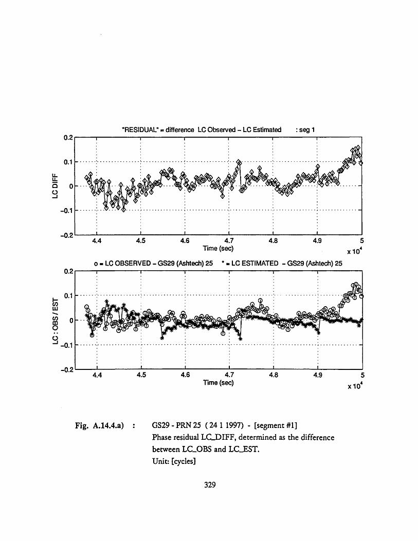
"RESIDUAL" = difference LC Observed - LC Estimated
4.4 4.5 4.6 4.7 4.8 4.9Time (sec)
o - LC OBSERVED - GS29 (Ashtech) 25 * - LC ESTIMATED - GS29 (Ashtech) 25
4.4 4.5 4.6 4.7 4.8 4.9 5Time (sec) x 104
Fig. A.14.4.a) GS29 - PRN 25 ( 24 1 1997) - [segment #1]Phase residual LCDIFF, determined as the differencebetween LC.OBS and LC.EST.Unit: [cycles]
329
'- .-
0.2
-0.1
-0.2
x 104
: seg 1

GS29 (Ashtech) PRN 25: Phase Error
* .
.: (
I ,
4.4 4.8 10-4
0.5
010C4.4 4.6 4.8 5
Power Spectra Density: Segment 1
S•: : ;
* .! ·- . ... . ........ ........
" " :1 ::::.* "................
le
10l
10-2 101
10-2
4.4 4.6 4.8Time (sec]
10" 10- 10-"x 10'
Fig. A.14.4.b) GS29 - PRN 25 (24 11997) - [segment #1]PSD of LCOBS, LCEST and LC..DIFF.
Unit: [cycles] 2
330
0.2
-0.1
-0.2
0.2
-0.1
-0.2
"'"' ' ' """
r··.··~···~.-.rr ·--· · ·· · ~···2.-.\r- '··-·~-~-~-~-··~r· · · · · ·· · · · ··· ····· · · · · · · · · · ~ · · ~·····
· ·. ·r . · .·r··~· · · . . · · ~..~· . · .. ·. · ·
,.rrr·r· · · · · · ·- · · · rr·r······ · · · r ·· · rr·· · · · · · · · · · · · · · · · · · · · ·· · · · · · · · · · · · · · · · · · · · ·
· · · · · · · · · · · · · · · · · · ·· · · · · · · r···
· · · · · · · · · · ·· · ·
101
10-'
=
f-4
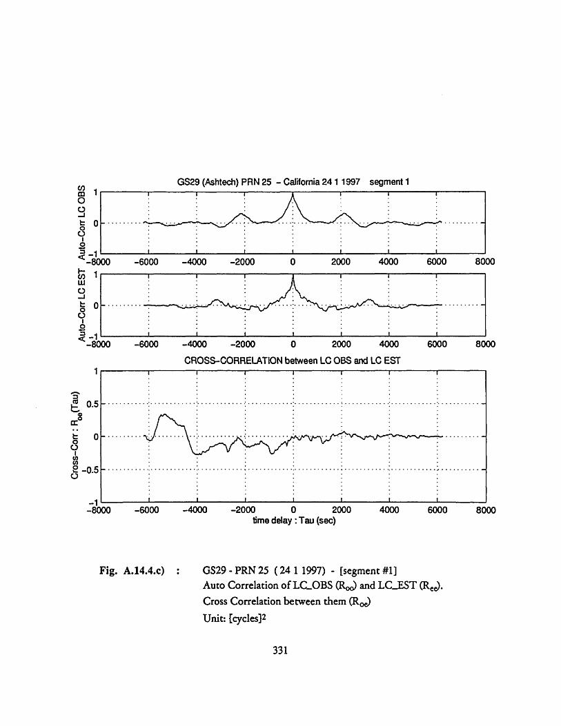
e/m 100-J" 0
o
I
GS29 (Ashtech) PRN 25 - Califomia 24 1 1997
-6000 -4000 -2000 0 2000 4000 6000
-M -6000 -4000 -2000 0 2000 4000 6000
CROSS-CORRELATION between LC OBS and LC EST
1
0.5
-6000 -4000
Fig. A.14.4.c)
-2000time delay :Tau (sec)
2000 4000 6000
GS29 -PRN 25 ( 24 1 1997) - [segment #1]Auto Correlation of LCOBS (RPo) and LC.EST (Ree.Cross Correlation between them (Roe)Unit: [cycles] 2
331
8000
8000
-0.5
_1-8000 8000
segment 1
-8000
-I
-a - a
.......... .............. .. ..
-..................................... ............ ...........

GS29 (Ashtech) PRN 25: Phase Error
4.4 4.6 4.8 5Time (sec) x 10
COHERENCE OF LC OBS and LC EST
-1
frequency [Hz]
frequency [Hz]
CROSS-SPECTRAL Power Density
10" 10 10"2
frequency [Hz]
Fig. A.14.4.d) GS29 - PRN 25 (24 1 1997) - [segment #1]Auto Spectral Power Density of LC..OBS (So) and of
LC.EST (See). Cross PSD between them (Soe)
Unit: [cycles]2
Coherence function of LC..OBS and LCEST
332
0.2
-0.1
-0.2
10-1
Auto-Spectral Power Density :seg 1
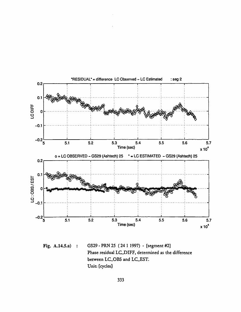
"RESIDUAL" = difference LC Observed - LC Estimated
Time (sec) x 10'
o = LC OBSERVED - GS29 (Ashtech) 25 * = LC ESTIMATED - GS29 (Ashtech) 25
5 5.1 5.2 5.3 5.4 5.5 5.6 5.7Time (sec) .,
A IJ
Fig. A.14.5.a) GS29 - PRN 25 ( 24 1 1997) - [segment #2]Phase residual LC...DIFF, determined as the differencebetween LCOBS and LC.EST.Unit: [cycles]
333
: seg 2

GS29 (Ashtech) PRN 25: Phase Error
. ........... ....... ........... .....%
:A,•:.~i ,I :,
5 5.2 5.4 5.6x 10'
5.2 5.4 5.6x 10⁴
5.5
. 5
Power Spectra Density: Segment 2
Mo 3
0-j2
o0 1CDCL
U-410-2
10
5.2 5.4 5.6Time [sec]
103
10-2
10- 2
x 10'
Fig. A.14.5.b) GS29- PRN 25 (24 1 1997) - [segment #2]Power Spectral Density of LCOBS, LCEST and LC..DIFF.Unit: [cycles] 2
334
¶i
0.2
-0.1
0.2
0.1
o
-0.1
0.1
0
-0.1
0',
..
......... ........
1.. . ... , :............ :: .......
".
-1
-1
-1
10
10
10
I Vi I >1111ii iI· \V···Ui·
.• :. :. :.. ..... .
I:: : ::: :11:111:.. ... ... :.:.:.:.:: .. . :::
,~ ,
·I ' """" ' ' """' ' " ";;'1
~· \I~· -·- --·-- ·-·-····-·- --·-- ·--·· ···--·· 1Lf ~
"" "'
I :;
-
I
.................... . . . . . . . . . . . .
L
10
.... . . . . i ....... ... ....
........................... ....
0.2
10.
...........................-
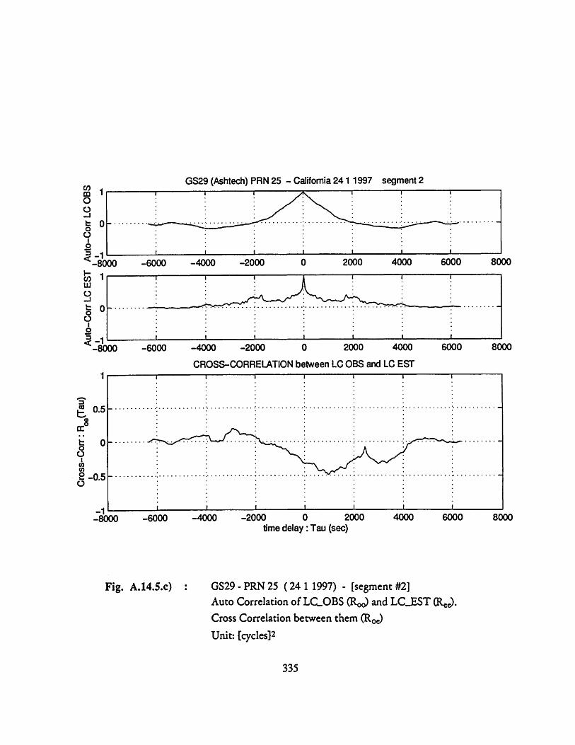
GS29 (Ashtech) PRN 25 - California 24 1 1997
-6000 -4000 -2000 0 2000 4000 6000
-4000 -2000 2000 4000 6000 804
CROSS-CORRELATION between LC OBS and LC EST
I I I Ii i i i ........... ..................... ..... ....... ..... .................... . .... .. ... ...
-6000 -4000 -2000time delay :Tau (sec)
2000 4000 6000 8000
Fig. A.14.5.c) GS29 - PRN 25 (24 1 1997) - [segment #2]Auto Correlation of LC..OBS (Ro~ and LC.EST (Re).
Cross Correlation between them (Ro)
Unit: [cycles] 2
335
MO
00
I0
00
S.
K0 -6000
w-J
0
-80
0.5
0
-0.5
_I
-8000-8000
segment 2M .
8000
00

GS29 (Ashtech) PRN 25: Phase Error
5 5.2 5.4 5.6Time (sec) x 10' frequency [Hz]
COHERENCE OF LC OBS and LC EST
V- V V ---V V
10-2frequency [Hz]
10- 1
CROSS-SPECTRAL Power Density
)-
frequency [Hz]
Fig. A.14.5.d) GS29 - PRN 25 ( 24 1 1997) - [segment #2]Auto Spectral Power Density of LC_OBS (Soo) and of
LC..EST (Se). Cross PSD between them (Soe)
Unit: [cycles] 2
Coherence function of LC.OBS and LCEST
336
0.8
o 0.6
o-
5 0.4U
0.2
n
10-4
Auto-Spectral Power Density :seg 2
·"''''"" ' ' """'· "''''·"1··.··. ·.·;.'.:: · · ·:··.·:-.' ~.·.:;'··· · · ·'····· ··· ······ · · -"··'···~..·..·.·. r ~·~~... r . .'. ~.'.:'.·rt
· '··· · ·
· ·· · · · · · · ·'····
· ·- · · ·'······ · · ·
· · ·- · ·· c-·-· · · · · · · · · ~···~····~·
'··· · · ·"····· · · ·'··· · · "'····· · · ·
-::· · · · I··:·:-:·-:·:i;"" ' ' """'
~a~t, ···
'
'
• o
10 :

"RESIDUAL" = difference LC Observed - LC Estimated
I.I I I I. I'""'~".. .. .. ......."...... .. ...... ...... ...... .. ... ....5.7 5.75 5.8 5.85 5.9 5.95 6 6.05 6.1 6.15 6.2
Time (sec)
o = LC OBSERVED - GS29 (Ashtech) 25 * = LC ESTIMATED - GS29 (Ashtech) 25
6.25x 10
5.7 5.75 5.8 5.85 5.9 5.95 6Time (sec)
6.05 6.1 6.15 6.2 6.25x 10⁴
Fig. A.14.6.a) : GS29 - PRN 25 (24 1 1997) - [segment #3]Phase residual LCDIFF, determined as the differencebetween LC.OBS and LC.EST.Unit: [cycles]
337
0.3
0.2
0.1
0
-0.1
-0.2
U.;3
0.2
0.1
-0.1
-0.2
.. I I . . . . .
:seg 3
I
I
m
I
-·..... ..............................·
X
ALNY'
· · · · · ·

GS29 (Ashtech) PRN 25: Phase Error Power Spectra Density : Segm 32
0.2 .................... ... .. .C1 1.5 *
n 0.1 ........ a V, 00 -
x 10x 10 .
0.20.1
W 00-J -0.1
-0.2
1.50-J
CO 0.5
a
5.7 5.8 5.9 6 6.1 6.2 10-4 10-3 10- 2 10"-
x 10'
0.2u- 0.1
j -0.1-0.2
LL
1.5
1-'
a.
5.7 5.8 5.9 6 6.1 6.2 10-4 10"3 10-2 101Time [sec] x 10
Fig. A.14.6.b) : GS29 - PRN 25 (24 1 1997) - [segment #3]Power Spectral Density of LC.OBS, LCEST and LCDIFF.Unit: [cycles] 2
338
" -
........ .............. ... . I
· ·. · - ·- · · · ·- · ......... ......~~'
· · ··
---- · · · · · · · ·-- · ·-- ·--- ·-' · · · · ·- · ·----------- · ·"' -·'---·-
··-- ·
-·· · · · · · ·-· · ·
.. ~..·..·.===·~rl·\ ·:··'·~-`-~-~·'-· . · ·-'··'·~·'·'· '·'-'·"'· \ ' ' `~~"" ' ' ""'
'"· ' ' ""'
: · -. · s-~;;.-J; ''-r~-~-r---;---;r- -- I··.-;·.-.-- · · · · · · · · · ·
· ·. · . · I·---··· · · · · · · ·
·
.:. .. . .. . .. . .. . . . . . .. . . .:. . . .. . .... . . .. .
. . . . . . . ... . . ., . .··. ······ : · ·-·· ·· ·- -.· .... ...... -'............
..· .=.·. '... .:. ... ·.... :.. .. . .; -- l-. ·-i;. ic- ··.-.-..·...

GS29 (Ashtech) PRN 25 - Califomia 24 1 1997 segment 3
-4000 -2000 0 2000 4000
CROSS-CORRELATION between LC OBS and LC ESTI &I I
L..
I II I I
-2000 0time delay :Tau (sec)
2000 4000
Fig. A.14.6.c) GS29 - PRN 25 (24 1 1997) - [segment #3]Auto Correlation of LC.OBS (Roo) and LCF.ST (Re).
Cross Correlation between them (Roe)
Unit: [cycles] 2
339
IM
0O
000oI
-6-6000
-bUUU
-4000 -2000 0 2000 4000 6000
6000
1
0.5
0o
2 -0.50.9-I
-6000 -4000 6000· · · 1
- I
,
L

GS29 (Ashtech) PRN 25 : Phase Error
... . . . . . . ... . . . . . .... . . .. . ... . . . . . . . .
S- ` i. .. 1.
.. . .. . .. . . . . . . . . . . . . . . . .. ." ° '
.. . .. . . . . . . . . . . . . . . .. . . . . . . . i. . . .
5.7 5.8 5.9 6 6.1 6.2Time (sec)
40C
--30(
"20(
8W 10(
1
x 10'
COHERENCE OF LC OBS and LC EST
Auto-Spectral Pow Density :seg 3
0i
. 1 zii ! ! ii !; · · · · · ·:•i . .. ... , !i iii i i i:ii0 ... ." i :: :.1::::i .~ .. : .iii:.. ...f. .:.i.i:I :\:::: ! ::: :;::. : Ij
104 10- 10-2
frequency [Hz]
CROSS-SPECTRAL Power Density
103 10-2frequency [Hz]
Fig. A.14.6.d)
10-1 10" 10- 10-2frequency [Hz]
GS29 - PRN 25 (24 1 1997) - [segment #3]Auto Spectral Power Density of LC..OBS (Soo) and of
LCEST (S). Cross PSD between them (Soe)
Unit: [cycles] 2
Coherence function of LC_OBS and LC_EST
340
0 0W-0.1
-0.2
10
0.8
0.6
0.4
0.2
nO.
10- 1• 1 1. . . . . . . . . .
0.3
0.2
• °
I -
[
U10
. .. • ° . . . . .... .. .. , . . . ....
.- -..;;- . , .; .; .. ';'. . .

GPS "OBSERVED" Phase Residuals for: COSO (Ashtech) PRN 30 - California 23 1 1997
1.2 1.4 1.6 1.8 2 2.2 2.4 2.6 2.8 3GPS "ESTIMATED" Phase Residuals computed from the analysis of SNR variation x 10'
1.2 1.4 1.6 1.8 2 2.2 2.4 2.6 2.8 3Comparison LC OBSERVED vs LC ESTIMATED x 10
1 1.2 1.4 1.6 1.8 2Time (sec)
2.2 2.4 2.6 2.8 3x 10'
Fig. A.15.1: Station: COSO - Satellite: PRN 30Data acquisition date 23 1 1997
The observed phase residual (LCOBS) is compared with themultipath phase error estimated from the SNR (LC...EST)Unit: [cycles)
341
o 0.1wc- 0.05wUn 0
O -0.05- -0.1
I I i a i a a a i .t
.- ..... . . . . . .. .. .
... . . ... ..!.1, ""..
r • r"I I I I . I .
I I I I I I I I
I.................. ......... ................. ..............I i..... .-··'··~ ·················· ·5... .... ...........:..... i.......... .......................................................
0.10.05
0
-0.05-0.1
0.10.05
0
-0.05-0.1
... . ................................. ............... i ..------ --. ...
. .. ..
.
I I I i i I i , I I
I I I n ......
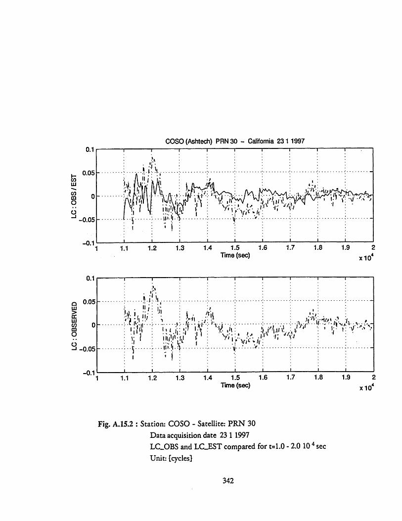
COSO (Ashtech) PRN 30 - Califomia 23 1 1997
1 1.1 1.2 1.3 1.4 1.5 1.6 1.7 1.8 1.9 2Time (sec) x 10'
[ I I -1
1.1 1.2 1.3 1.4 1.5 1.6 1.7 1.8 1.9 2Time (sec) x 104
Fig. A.15.2 : Station: COSO - Satellite: PRN 30Data acquisition date 23 1 1997LCOBS and LC.EST compared for t=1.0 - 2.0 10 4 sec
Unit: [cycles)
342
0.05
0
-0.05
-0.1
S. . . . .
FI. I I I I I I1
i

"RESIDUAL" = difference LC Observed - LC Estimated - 23 1 1997
1 1.1 1.2 1.3 1.4 1.5 1.6 1.7 1.8 1.9 2Time (sec) x 10
o = LC OBSERVED - COSO (Ashtech) 30 * - LC ESTIMATED - COSO (Ashtech) 30
1 1.1 1.2 1.3 1.4 1.5 1.6 1.7 1.8 1.9 2Time (sec) x 10'
Fig. A.15.3.a) COSO - PRN 30 (23 1 1997) - [segment 1]Phase residual LC..DIFF, determined as the differencebetween LCOBS and LC.EST.Unit: [cycles]
343
0.15
0.1
0.05
0
-0.05
-0.1
0.15
0.1
S0.05
w
o. -0.05-J
-0.1

COSO PRN 30 (23 1 1997): Phase Error
1.2 1.4 1.6 1.8x 10'
1.2 1.4 1.6 1.8
n10-le
0
Power Spectra Density
...
.... :: . . . ...... . . . . ....
; " ' : ; 5 " " " '1" . . ......'"v i " ' ?' """i' : :: ::
"\ "
:/: ::: :• (-,. :t•:,:-.·. -·--. . -Li - ! ! !•!ii?·
10
10 4
10-210
10-2
0-110
10- 1
x 10'
1 1.2 1.4 1.6Time [sec]
1.8 2x 10*
0.4
0.2
loe-3 -2
10- 10-~ 2
Frequency [Hz]
Fig. A.15.3.b) COSO- PRN 01 (23 11997) - [segment 1]PSD of LC.OBS, LC_..EST and LC.DIFF.
Unit: [cycles] 2
344
..........l....... .......... ....... .........l
......... .......................
........................ ....i......... ..
t -- ---- ---
0.10.05
0
-0.05-0.1
0.050
-0.05-0.1
. . . . .:.. . : . . . . .
0.10.05
0-0.05
-0.1
10- 1
- -- · -- --- ~- -·
........... ...... ,......... ....
..... .. .. .... .. . ...... ... .... .. ..
.......·...... ......:...................
1.2 1.4 1.6 1.8
. . ... . ..
. . . . - .
x
104
' i
z
I
x
10
4
· '
· ·
· ·... ,
· .· .
i
10 -3
..'AA
"'"
'
"'·.-. ·. ·. I·
· ·· ·
·-· ·
·.--- ·-· ·
· ·· ·
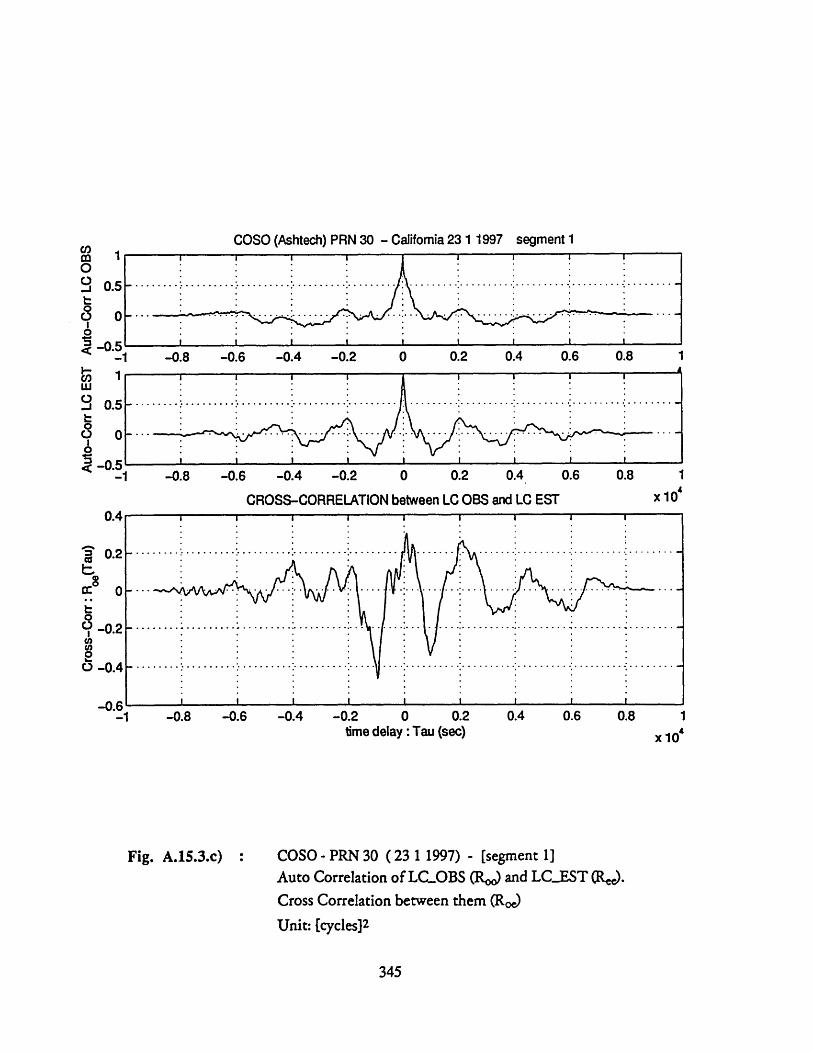
COSO (Ashtech) PRN 30 - California 23 1 1997 segment 1
0.5
0
-n r.
-1
-1 -_0. -U.b -U.4 -U.2 U U.Z U.4 U.b U.0 1
CROSS-CORRELATION b
T x 10
0.2
a: 0
00 -0.2
0CA
0-0.
-0.8 -0.6
Fig. A.15.3.c)
-0.4 -0.2 0 0.2 0.4 0.6 0.8 1time delay : Tau (sec)
COSO - PRN 30 (23 1 1997) - [segment 1]Auto Correlation of LC..OBS (R) and LC..EST (Re.Cross Correlation between them (Ro
Unit: [cycles] 2
345
.I I I I . . .. I..
0 0.2 0.4 0.6 0.8 1-0.8 -0.6 -0.4 -0.2
I-- - tI I
I I I I I
-1
x 10'
_ ·
4
-
-
-
,,P,·r ~ Rt•R-R3RRIAT(3 h~·~ twl~-·n LC -~ -1 n CI='"x
· · · · · · · ·i
A c

COSO (Ashtech) PRN 30 (23 1 1997): Phase Error0.1
0.05
0
-0.05
-0.11 1.2 1.4 1.6
Time (sec)
1
8
Uo
c')"1
1.8 2
x 104
COHERENCE OF LC OBS and LC EST
-1
frequency [Hz]
frequency [Hz]
CROSS-SPECTRAL Power Density
10" 10-" 10"frequency [Hz]
Fig. A.15.3.d) COSO - PRN 30 (23 1 1997) - [segment 1]Auto Spectral Power Density of LC_OBS (Soo) and of
LC...EST (See). Cross PSD between them (Soe)Unit: [cycles] 2
Coherence function of LCOBS and LC..EST
346
-I
10'
Auto-Spectral Power Density

0.10.05
0-0.05-0.1
0.10.05
0-0.05-0.1
GPS "OBSERVED" Phase Residuals for: COSO (Ashtech) PRN 30 - California 24 1 1997
.... ........ .....
.I
r I .. . . . I ................... ......... ............ ...... :....... ...- ...... ... . . ...
It s I III
1.2 1.4 1.6 1.8 2 2.2 2.4 2.6 2.8 3GPS "ESTIMATED" Phase Residuals computed from the analysis of SNR variation x 10
1.2 1.4 1.6 1.8 2 2.2 2.4 2.6 2.8 3Comparison LC OBSERVED vs LC ESTIMATED x 104
0.10.05
0-0.05-0.1
1 1.2 1.4 1.6 1.8 2Time (sec)
2.2 2.4 2.6 2.8
Fig. A.16.1: Station: COSO - Satellite: PRN 30Data acquisition date 24 1 1997The observed phase residual (LC.OBS) is compared with themultipath phase error estimated from the SNR (LCEST)Unit: [cycles]
347
I I __ I F
................... .. . .. . .. .. .. .. .. .. .
.......... .......... ...... I.. .......... .......... .......... ....................-... ... ... .... .. ... ..... ... ..... .... .. .... . ..... ... ... ... .. .. ...
I I I I I I
S... ..... ..... ..... .. .. ......... ..
.................. .... .... .
3
x 104
I I I I I I I I I
c
!I

COSO (Ashtech) PRN 30 - Califomia 24 1 1997
1 1.2 1.4 1.6 1.8 2 2.2 2.4 2.6 2.8 3Time (sec) x 10
0.15
0.1
0.05
0
-0.05
-0.1
1 1.2 1.4 1.6 1.8 2Time (sec)
2.2 2.4 2.6 2.8
Fig. A.16.2 : Station: COSO - Satellite: PRN 30Data acquisition date 24 1 1997LCOBS and LCEST compared for t=1.0 - 2.0 10 4 sec
Unit: [cycles]
348
IIII II. .......... ........ .: ......... .......... .......... ....... _" .... ..... . ... :. II . ..
I -
3x 10
-----

"RESIDUAL" - difference LC Observed - LC Estimated - 24 1 1997
1.1 1.2 1.3 1.4 1.5 1.6 1.7 1.8 1.9Time (sec) x 10'
o = LC OBSERVED - COSO (Ashtech) 30 * = LC ESTIMATED - COSO (Ashtech) 30I. I I II I~ I I I I
1 1.1 1.2 1. 1.4 1. 1.6 1.7 1.8 1.9 21 1.1 1.2 1.3 1.4 1.5 1.6 1.7 1.8 1.9 2
Time (sec) x 104
Fig. A.16.3.a) COSO - PRN 30 (24 1 1997) - [segment 1]Phase residual LC...DIFF, determined as the differencebetween LCOBS and LCEST.Unit: [cycles]
349
0.15
0.1
0.05
0
-0.05
-0.1
0.15
0.1
0.05
00 -0.05
-0.1-0.1
* ... I 1
_ · · _· · ·
i

COSO PRN 30 (24 1 1997): Phase Error
0.1cn 0.050 0
-3 -0.05
-0.1
1 1.2 1.4 1.6 1.8
0.10.05
0-0.05
-0.1
x 10'103
n1.2 1.4 1.6 1.8
0.1u. 0.055 0
0 S-0.05-0.1
x 10'
1 1.2 1.4 1.6Time [secJ
10-4
1.8 2
x 10'
10-2
10-3 10-210
Frequency [Hz]
Fig. A.16.3.b) COSO-PRN 01 (24 1 1997) - [segment 1]PSD of LC.OBS, LC.EST and LCJDIFF.Unit: [cycles] 2
350
I..I.. . . . . . . . . . . .. . ...........r .3 . .... ...4 -. .............. .: ..............
...... ... ·.. . Lir .. .. . . . . . . . . . . .
..
: ..
I: :,. .....:1:'
." . · r..~.~ .I......
0- 1
10- 1
-1
Power Spectra Density
I
.. . . ... . . . .. . . . .. . . .
.. ... .......... ... ...... ..... .... ..... ... ... .... ...... ... ...
X
104
" ' ':: : : : : '' ': ' ' "':':
. . ... ... . . . .. .. . . . ...
. . . . .. . . . .
. ... 1...:.... = ·- t.. ....... . . .. ·....• ::.;L~ .....
... . . . . ., . .. . . ... . . .
. . . . . . . . . . . . . . . . . . . . . . . . ... ........... ........................
x
104
· ·
· '
t .·. ·. ·. ·h· ·· ·· ·
· · ·
· ·
10 -4

COSO (Ashtech) PRN 30 - Caifomia 24 1 1997 segment 1et
-0.8 -0.6 -0.4 -0.2 0 0.2 0.4 0.6 0.8 1
-0.8 -0.6 -0.4 -0.2 0 0.2 0.4 0.6 0.8 1
CROSS-CORRELATION between LC OBS and LC EST x 10'
-0.8 -0.6 -0.4 -0.2
Fig. A.16.3.c)
0 0.2 0.4 0.6 0.8 1time delay :Tau (sec)
COSO - PRN 30 ( 24 1 1997) - [segment 1]Auto Correlation of LC.OBS (Roo) and LC..EST .
Cross Correlation between them (Ro)
Unit: [cycles] 2
351
S1O
-J
0o
I0
I1-1-1
0.5
-0.5
I1
I I I I I I I I I
I I I II ~ l~I-1l
1
x 10'
<-1
-

COSO (Ashtech) PRN 30 (24 1 1997): Phase Error
1 1.2 1.4 1.6Time (sec)
1.8 2
x 104
COHERENCE OF LC OBS and LC EST1500
t' 1000
0
" 500CL
n
-1
frequency [Hz]
Fig. A.16.3.d)
frequency [Hz]
CROSS-SPECTRAL Power Density
10 10- 2
frequency [Hz]101
COSO - PRN 30 (24 1 1997) - [segment 1]Auto Spectral Power Density of LC.OBS (So) and of
LC..EST (Se). Cross PSD between them (Soe)
Unit: [cycles] 2
Coherence function of LCOBS and LC.EST
352
Auto-Spectral Power DensityI
10"

Appendix B
353
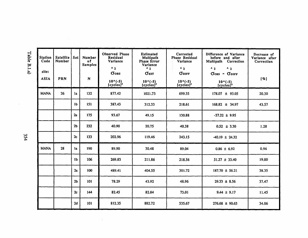
tIA
b'
Observed Phase Estimated Corrected Difference of Variance Decrease ofStation Satellite Set Number Residual Multipath Phase Residual before and after Variance afterCode Number of Variance Phase Error Variance Multipath Correction Correction
Samples VarianceA 2 A2 2 A2 A2
site: GOBS GEST (TDIFF TOBS - NDIFF
ASIA PRN N [%]ASIA PRN A(5) 10^(5) 1A(-) 10A(-.5) 1%[cycles]' [cycles] 2 [cycles] [cycles?)
MANA 26 la 132 877.42 1021.73 699.35 178.07 ± 93.05 20.30
lb 151 387.43 312.33 218.61 168.82 ± 34.97 43.57
2a 175 93.67 49.15 130.88 -37.22 ± 9.95
2b 232 40.90 20.75 40.38 0.52 ± 3.30 1.28
2c 133 202.96 119.46 243.15 -40.19 + 24.32
MANA 28 la 190 89.90 30.48 89.04 0.86 + 6.92 0.96
lb 106 269.83 211.86 218.56 51.27 + 33.40 19.00
2a 100 489.41 404.55 301.72 187.70 ± 56.21 38.35
2b 101 78.29 43.92 48.96 29.33 ± 8.56 37.47
2c 144 82.45 82.84 73.01 9.44 ± 9.17 11.45
2d 101 812.35 882.72 535.67 276.68 ± 90.63 34.06-ii i1
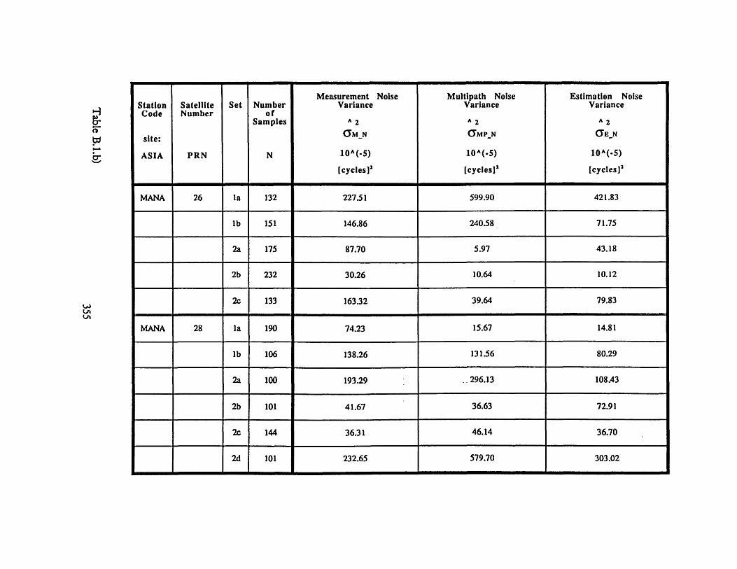
t•t•H
t.
U'
Measurement Noise Multipath Noise Estimation NoiseStation Satellite Set Number Variance Variance VarianceCode Number of
Samples ^ 2 ^ 2 A 2
site: GMN GMPN GEN
ASIA PRN N 10^(-5) 10^(-5) 10^(-5)
[cycles]' [cycles]2 [cycles] 2
MANA 26 la 132 227.51 599.90 421.83
lb 151 146.86 240.58 71.75
2a 175 87.70 5.97 43.18
2b 232 30.26 10.64 10.12
2c 133 163.32 39.64 79.83
MANA 28 la 190 74.23 15.67 14.81
lb 106 138.26 131.56 80.29
2a 100 193.29 .. 296.13 108.43
2b 101 41.67 36.63 72.91
2c 144 36.31 46.14 36.70
2d 101 232.65 579.70 303.02
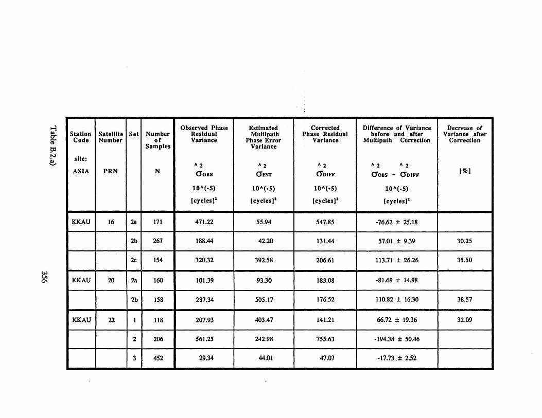
Observed Phase Estimated Corrected Difference of Variance Decrease ofStation Satellite Set Number Residual Multipath Phase Residual before and after Variance afterCode Number of Variance Phase Error Variance Multipath Correction Correction
Samples Variance
site:A 2 A 2 A 2 A 2 ^2
ASIA PRN N ooas Esr OCDIFF COBS - (DI
10^(-5) 10^(-5) 10^(-5) 10^(-5)
[cycles]' [cycles]' [cycles]2 [cycles])
KKAU 16 2a 171 471.22 55.94 547.85 -76.62 ± 25.18
2b 267 188.44 42.20 131.44 57.01 ± 9.39 30.25
2c 154 320.32 392.58 206.61 113.71 ± 26.26 35.50
KKAU 20 2a 160 101.39 93.30 183.08 -81.69 ± 14.98
2b 158 287.34 505.17 176.52 110.82 ± 16.30 38.57
KKAU 22 1 118 207.93 403.47 141.21 66.72 ± 19.36 32.09
2 206 561.25 242.98 755.63 -194.38 ± 50.46
3 452 29.34 44.01 47.07 -17.73 .± 2.52
,-3
0
0v
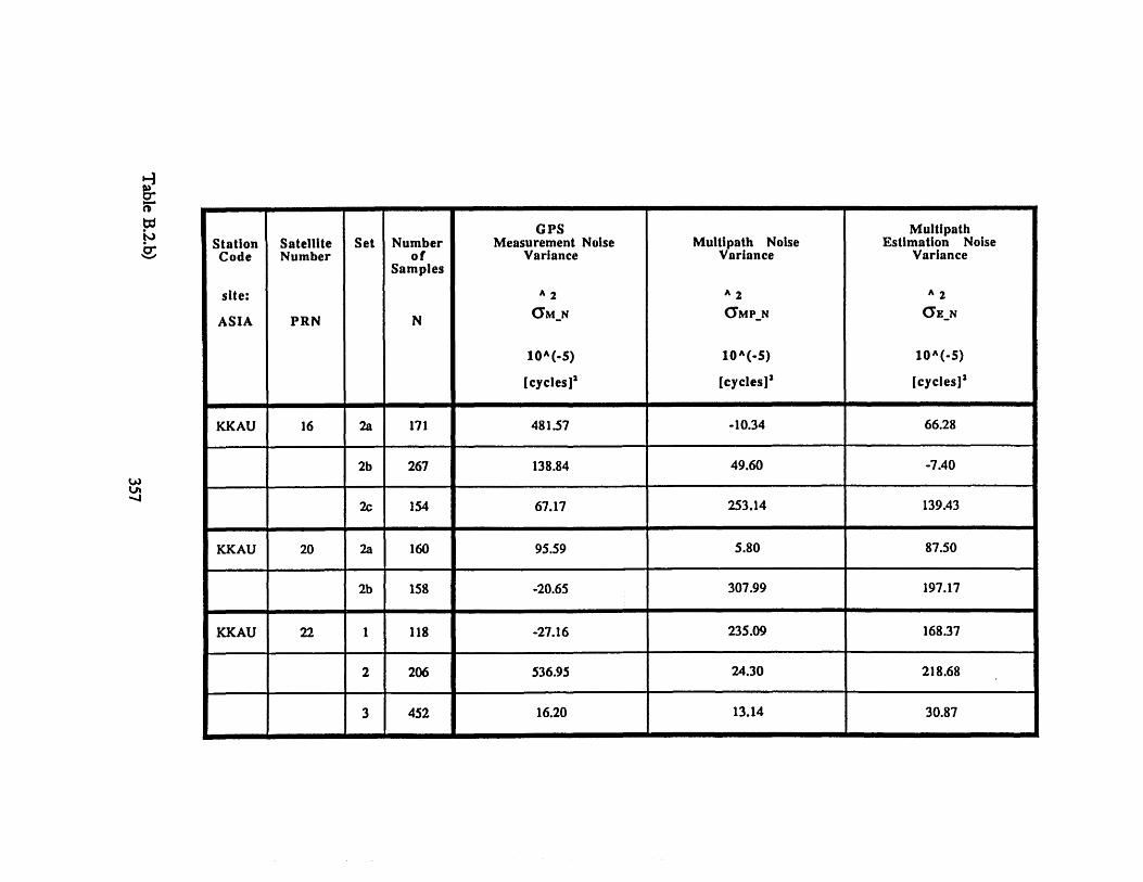
WE.
tb30,
rl.
GPS MultipathStation Satellite Set Number Measurement Noise Multipath Noise Estimation NoiseCode Number of Variance Variance Variance
Samples
site: ^ 2 A 2 A 2
ASIA PRN N GMN MPN (EEN
10A(.5) 10^(-5) 10A(-5)
[cycles]' [cycles]' [cycles]'
KKAU 16 2a 171 481.57 -10.34 66.28
2b 267 138.84 49.60 -7.40
2c 154 67.17 253.14 139.43
KKAU 20 2a 160 95.59 5.80 87.50
2b 158 -20.65 307.99 197.17
KKAU 22 1 118 -27.16 235.09 168.37
2 206 536.95 24.30 218.68
3 452 16.20 13.14 30.87- -i

Observed PhaseResidualVariance
^ 2
10^(-5)
[cycles]'
,m
L0n
EstimatedMultipath
Phase ErrorVariance
A 2
GE~r
10^(-5)
[cycles]'
2459.69
306.73
95.13
83.64
160.31
597.31
255.62
CorrectedPhase Residual
Variance
A 2ODIFF
10^(-S)
[cycles]'
1089.03
413.08
124.95
165.37
192.40
297.77
105.95
Difference of Variancebefore and after
Multipath Correction
A 2 2GoBS - GDIFF
10^(-5)
[cycles]'
995.22 + 130.22
117.71 + 49.58
3.29 ± 15.51
-88.10 ± 14.71
68.19 ± 18.15
99.82 + 21.43
56.66 ± 5.11
Decrease ofVariance after
Correction
[%]
47.75
22.18
2.56
26.17
25.11
34.84
2084.25
530.79
128.23
77.28
260.59
397.59
162.60
StationCode
site:
LIGO
00280036
00280036
00280036
SatelliteNumber
PRN
09
15
25
Set
1I
2
3
4
1
2
Numberof
Samples
N
208
160
126
124
286
256
254
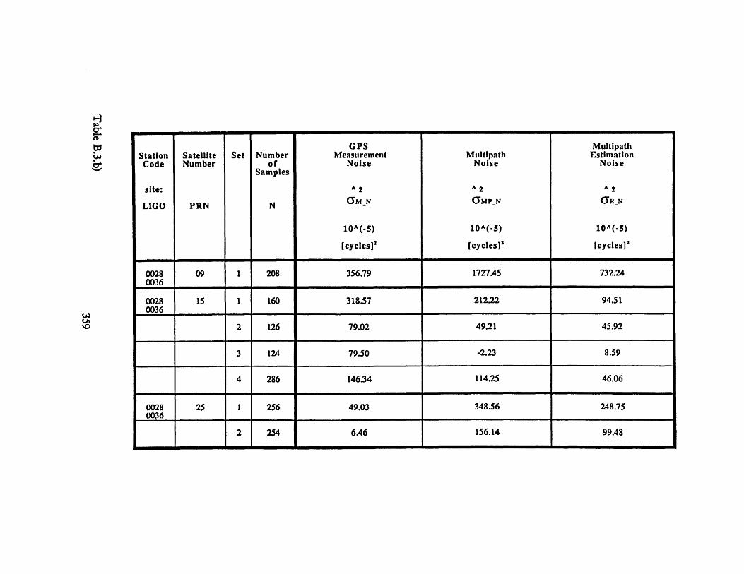
IA
LA'w0cr
GPS MultipathStation Satellite Set Number Measurement Multipath EstimationCode Number of Noise Noise Noise
Samples
site: ^ 2 ^ 2 A 2
LIGO PRN N OMN MP-N (EN
10^(-5) 10A(5) 10^(-5)
[cycles]' [cycles]' [cycles] 2
0028 09 1 208 356.79 1727.45 732.240036
0028 15 1 160 318.57 212.22 94.510036
2 126 79.02 49.21 45.92
3 124 79.50 -2.23 8.59
4 286 146.34 114.25 46.06
0028 25 1 256 49.03 348.56 248.750036
2 254 6.46 156.14 99.48

EstimatedStation Satellite Set Number Observed Phase Multipath Corrected Difference of Variance Decrease ofCode Number of Residual Phase Error Phase Residual before and after Variance after
Samples Variance Variance Variance Multipath Correction Correction
data:A 2 A 2 A 2 A 2 ^2
LIGO PRN N OoBS GEST O'DIFF OOBS - ODIFF [%]
10^(-5) 10^(-5) 10^(-5) 10^(-5)
[cycles]' [cycles]2 [cycles]? [cycles] 2
LI 09 1 208 280.00 200.00 210.00 70.59± 2.35 25.38
L2 09 1 208 420.00 81.89 280.00 140.00± 2.20 34.18
GPS Multipath MultipathStation Satellite Set Number maesurement Variance estimation noiseCode Number of noise noise Variance
SamplesLIGO A 2 A 2 A 2
PRN N (MN (MPN EN
Ll 09 1 208 140.00 130.00 63.33
L2 09 1 208 310.00 110.00 -30.80
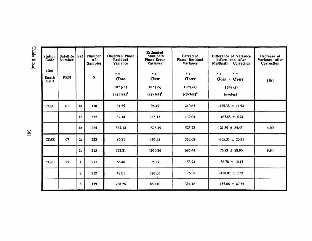
EstimatedStation Satellite Set Number Observed Phase Multipath Corrected Difference of Variance Decrease ofCode Number of Residual Phase Error Phase Residual before and after Variance after
Samples Variance Variance Variance Multipath Correction Correction
site:^ 2 ^ 2 ^ 2 A 2 ^2
South PRN N GOBs (EST (DIFF GOBS - (DIFFCalif [%]10^(.5) 10^(-5) 10^(5S) 10^(5)
[cycles]' [cycles]' [cycles]) [cycles]'
COSE 01 la 170 81.25 96.49 210.63 -12938 + 14.94
lb 332 32.14 115.13 139.01 -167.88 + 6.24
Ic 224 547.12 1576.49 525.23 21.89 + 84.43 4.00-I
COSE 07 2a 233 86.71 195.98 352.02 -26531 + 20.21
2b 215 772.21 1910.36 695.44 76.73 ± 88.90 9.94
COSE 25 1 211 66.46 75.87 153.24 -86.78 + 10.17
2 212 48.01 192.05 176.02 -128.01 + 7.63
3 179 238.26 880.10 394.16 -155.86 + 47.53

ipH0\
it
oCt,•
GPS MultipathStation Satellite Set Number Measurement Noise Multipath Noise Estimation NoiseCode Number of Variance Variance Variance
Samples
site: ^ 2 ^ 2 A 2
South PRN N GMN (MPN GENCalif Calif 0 ^ (-5) 10 ^ (-5) 10 ^ (-5)
[cycles]' [cycles]2 [cycles]2
COSE 01 la 170 97.70 -16.45 112.94
lb 332 28.01 4.12 111.01
Ic 224 252.07 799.19 777.30
COSE 07 2a 233 121.38 -34.66 230.64
2b 215 -222.26 1008.77 929.60
COSE 25 1 211 71.91 -5.46 81.33
2 212 15.99 32.02 160.03
3 179 -155.86 362.12 517.88

EstimatedStation Satellite Set Number Observed Phase Multipath Corrected Difference of Variance Decrease ofCode Number of Residual Phase Error Phase Residual before and after Variance after
Samples Variance Variance Variance Multipath Correction Correction
site:A 2 A 2 A 2 A 2 A 2
South PRN N Goas OGEST DIFF GOBS - GDIFFCalif [%10A(-5) 10A(.5) 10A(-5) 10A(.5)
[cycles]' [cycles]' [cycles]' [cycles])
GS29 01 la 173 50.94 56.28 90.32 -39.38 + 7.46
lb 332 106.06 2.95 114.65 -8.59 ± 1.97
Ic 219 635.20 1046.25 529.37 105.83 + 33.70 16.66
GS29 07 2a 234 30.19 7.75 43.50 -13.32 + 2.10
2b 211 797.58 1221.09 631.62 165.96 ± 48.85 20.81
GS29 25 1 208 123.95 59.26 176.77 -52.82 ± 11.76
2 212 178.50 4.62 192.37 -13.87 ± 4.01
3 173 319.50 297.42 130.28 189.22 + 22.96 59.22
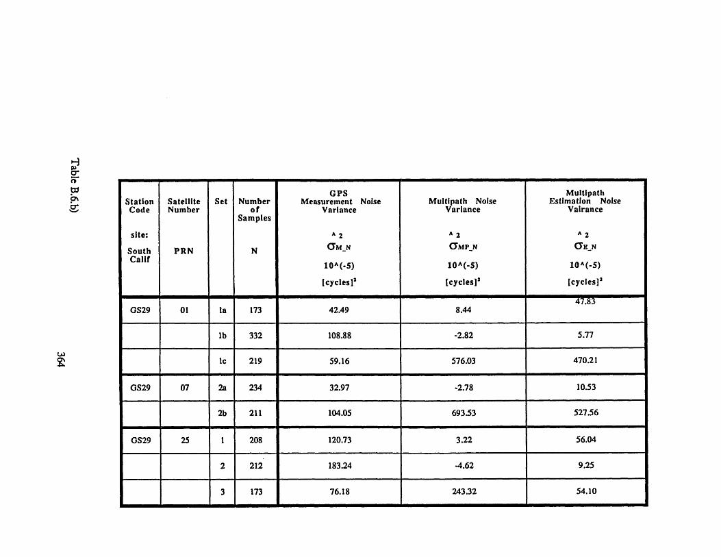
GPS MultipathStation Satellite Set Number Measurement Noise Multipath Noise Estimation NoiseCode Number of Variance Variance Vairance
Samples
site: ^ 2 ^ 2 A 2
South PRN N - (MPN (EN
Calif10^(-5) 10^(-5) 10^(-5)
[cycles] 2 [cycles]' [cycles]2
GS29 01 la 173 42.49 8.44
lb 332 108.88 -2.82 5.77
Ic 219 59.16 576.03 470.21
GS29 07 2a 234 32.97 -2.78 10.53
2b 211 104.05 693.53 527.56
OS29 25 1 208 120.73 3.22 56.04
2 212 183.24 -4.62 9.25
3 173 76.18 243.32 54.10- - -
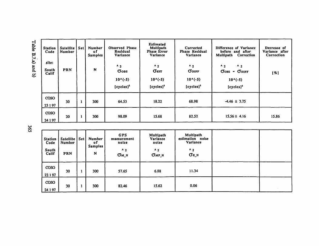
C,
0w
U.
EstimatedStation Satellite Set Number Observed Phase Multipath Corrected Difference of Variance Decrease ofCode Number of Residual Phase Error Phase Residual before and after Variance after
Samples Variance Variance Variance Multipath Correction Correction
site:^ 2 ^ 2 A 2 A 2 A 2
South PRN N Goss EST MGDIFF (OBS - ODIFFCalif [%J10^(-5) 10^(-5) 10^(-5) 10^(.5)
[cycles]2 [cycles]' [cycles]) [cycles]'
COSO30 1 300 64.53 18.22 68.98 -4.46 ± 3.75
23 1 97
COSO30 1 300 98.09 15.68 82.52 15.56 ± 4.16 15.86
24 197
GPS Multipath MultipathStation Satellite Set Number maesurement Variance estimation noiseCode Number of noise noise Variance
SamplesSouth ^ 2 ^ 2 A 2Calif PRN N GM N GOMPN OEN
COSO30 1 300 57.65 6.88 11.34
23 1 97
COSO30 1 300 82.46 15.62 0.06
241 97

366

Appendix C
367

FFTobs est diff.m
t% This program computes the Power Spectral Density of the time seriesS LC_ OBS, LC_EST and LC DIFF
clear
load SAT ESTload SAT _OBS
Nl-length(SAT OBS(:,1));N2-length(SAT_EST(:,1));
index-0;
hours-18;minutes-45;
epoch - SAT OBS(:,i);time _sec= (epoch-l)*30+hours'3600+minutes*60;SAT_0BS(:,l)-time sec;
for j-i:Nlfor i-1:N2
if SAT0OBS(j, 1)-SATEST (i, 1)index-index+l;SAT D 3(index,1)-SAT OCBS(j,1);SAT D 3(index,2)-SAT OBS(j,4)-SAT_EST(i,7);SAT 0 1(index,1)-SAT OBS(j, 1);SAT E 2(index,1)-SAT EST(i,1);SAT 0 1(index,2)-SATC BS(j,4);SAT E 2 (index, 2)-SAT EST (i, 7);
end
endend
SAT 1-SAT 0 1;SAT 2-SAT E 2;SAT 3-SAT D 3;
n-length(SAT 2(:,l));dt-30;m-n/2;
SATE (r,l)-SAT 2(1,1);SAT _O (r, 1)-SAT 2(1,1);SAT D(r,1)-SAT 2(1,1);
SAT 0(r,2)-SAT 1(1,2);SAT E(r,2)-SAT 2(1,2);SAT D(r,2)-SAT 3(1,2);
368
~--·-IIPPIII~IPIl~··~IPPPIPPPIIIIIIIPIIIP

for ind-2:nr=r+1;SAT 0(r,1)-SAT 2(ind,1);SAT E (r, 1)-SAT 2 (ind, 1);SAT D(r,1)-SAT 2(ind,1);
SAT O(r,2)-SAT_ (ind,2);SATE (r, 2) -SAT 2 (ind, 2);SAT D(r,2)-SAT 3(ind,2);
if SAT 2(ind,1)>SAT 2(ind-1,1)-+dtt miss-SAT 2(ind)-SAT 2(ind-1);n miss-t miss/dt-1;for i-1:nmiss+l
SAT O(r,1)-SAT 2(ind-1,1) +dti;SAT E(r,1)-SAT 2(ind-1,1)+dt*i;SAT D(r,1)-SAT 2(ind-, 1)+dt*i;
SAT 0(r,2)-SAT 1(ind-1,2)+i*(SAT_1 (ind,2)-SAT 1(ind-1,2))/ (n_miss+1);SAT E(r,2)-SAT-2(ind-1,2)+i*(SAT 2(ind,2)-SAT 2(ind-1,2))/(nmiss+l);SAT D(r, 2) -SAT 3(ind-i,2)+i*(SAT_3(ind,2)-SAT 3(ind-1,2))/ (n_miss+l);
if i<n miss+lr-r+l;end
end
end
end
N-r;
dt-30;Ny-n/2+1;fNy - 1/(2*dt);T - n*dt;df-fNy/(Ny-1);f-[0 :df: fNy];
norm E -( SAT E(:,2)-mean(SAT E(:,2)) );norm 0 ( SAT_0(:,2)-mean(SAT_0(:,2)) );norm DIFF-( SATD(:,2)-mean(SAT D(:,2)) );
FTEST - fft(norm E);FTOBS - fft(norm 0);FT DI-F - fft(norm DIFF);
? FT EST-FT EST.*conj(FTEST)./n;P FT OBS-FT OBS.'conj(FT_OBS)./n;P_FTDIFF-FTDIFF. *conj (FTD-) ./n;
figure (1)clf
subplot (3,2,1)plot(SAT0O(:,1), SAT_O(:,2),'-.')holdgridylabel(' LC OBS ')title(' COSE (Trimble) PRN 25: Phase Error')
369

subplot (3, 2, 2)se.milogx(f,PFTOBS(l:Ny)*dt,'-.');holdgridylabel(' PSD of LC OBS')title ('?ower Spectra Density: Segment 3')
subplot (3, 2, 3)plot (SATE(:, 1l), SATE(:,2))holdgridylabel('LC EST ')
subplot (3, 2, 4)semilogx(f,PFTEST(1:Ny) dt);holdgridylabel(' PSD of LC EST')
subplot (3,2,5)plot (SAT D(:, 1), SAT D(:,2))holdgridylabel('LC DIFF')xlabel('Time [sec]')
subplot (3, 2, 6)semilogx(f,PFT_DIFF (l:Ny)dt);holdgridylabel(' PSD of LC DIFF')
return
370

% Auto Cross CORR..m
This program computes the Auto correlation of the two time series% LCOBS, LCEST and their Cross correlation
clear
load SAT ESTload SAT OBS
clear
load SAT ESTload SAT OBS
Nl-length (SAT OBS (:,));N21length(SAT EST(:,1));
index-0;
hours-18;minutes-45;
epoch - SAT_OBS(:,l);time sec= (epoch-) *30+hours*3600+minutes*60;SAT OBS (:, 1)-timesec;
for j-l:Nlfor i-L:N2
if SATOBS(j,l)-SAT EST(i,1)index-index+l;SATD_3(index,l)-SAT_OBS(j,1);SATD_3(index,2)-SAT OBS(j,4)-SAT.EST(i,7);SAT 0 _l(index,l)-SATOBS(j,1);SAT E 2(index,l)-SAT EST(i, 1);SAT 0 1 (index,2)-SAT OBS (j, 4);SAT E_2 (index, 2) -SAT EST (i, 7);
end
endend
SAT 1=SAT 0 1;SAT 2=SAT E 2;SAT_3-SAT D 3;
n-length (SAT2 (:, 1));dt-30;m-n/2;
371

r-1;
SAT E(r,1)-SAT 2(1,1);SAT-0 (r, 1)-SAT 2(1,1);SAT D(r, 1)-SAT 2(1,1);
SAT O(r,2)-SAT 1SAT E (r,2)-SAT 2SAT D(r,2)-SAT 3
(1,2);(1,2);(1,2);
for ind-2:nr-r+1;SAT O(r,1)-SAT 2(ind, 1);SAT E(r, 1)-SAT 2(ind, 1);SAT D (r, 1)-SAT 2 (ind, 1);
SAT 0(r, 2)-SAT1 (ind, 2);SAT E(r,2)-SAT 2 (ind,2);SAT D(r,2)-SAT 3(ind,2);
if SAT 2(ind,1)>SAT 2(ind-1,1)+dtt miss-SAT 2(ind)-SAT 2(ind-1);n miss-t miss/dt-1;for i-l:n miss+l
SAT_ (r,l)-SAT 2(ind-1,1)+dt'i;SATE(r,1)-SAT 2(ind-!,l)+dt*i;SAT D(r,1)-SAT 2(ind-1,1)+dt*i;
SAT 0(r,2)-SAT 1(ind-1,2)+i*(SAT_1(ind,2)-SAT_ (ind-1,2))/(n miss+1);SAT_ (r, 2)-SAT 2(ind-1,2)+i(SAT_2 (ind, 2)-SAT_2 (ind-1, 2))/(nmiss+l) ;SATD (r,2)-SAT3 (ind-1,2)+i"(S-AT 3(ind,2)-SAT_3(ind-1,2))/(nmiss+1);
if i<n miss+1r-r+i;end
end
end
end
N-r;
figure (I)clf
subplot(4,1,1)x-SAT 0(:,2);c-xcorr (x,'coeff');Tau-N*30;L--Tau+30 :30 :Tau-30;plot(L',c)holdgridylabel('Auto-Corr LC OBS')title('COSE (trimble) ?RN 25 - California 23 1 1997 segment 1')
subplot (4, 1,2)y-SAT_E ( :,2);c-xcorr (y, 'coeff');Tau-N *30;
372

L--Tau+30 :30 :Tau-30;plot (L', c)holdgridylabel('Auto-Corr LC EST')
subplot (2, 1, 2)x-SAT 0(:,2);y-SAT E(:,2);c-xcorr (x, y, 'coeff');Tau=N*30;L--Tau+30: 30: Tau-30;plot (L', c)holdgridylabel(' Cross-Corr : R_o_e(Tau)')xlabel(' time delay : Tau (sec) ')title(' CROSS-CORRELATION between LC OBS and LC EST ')return
373

% SP CORR obs est.m.m
This program computes the AUTO Spectral Density of the two time seriesLC OBS, LC EST and their CROSS Spectral Density from the correlationfunctions.
clear
format long
load SAT ESTload SAT_0BS
N1-length(SAT OBS (:,1));N2-length(SATEST (:, ));
index-0;
hours-18;minutes-45;
epoch - SATCBS(:,I);time sec- (epoch-1)*30+hours*3600+minutes*60;SAT _OBS(:,l)-time sec;
for j-l:N1for i-I:N2
if SAT OBS(j,1)--SAT EST(i,l)index-indexi1;SAT D 3(index,1)-SAT OBS(j,1);SAT D 3(index,2)-SATOBS (j,4)-SAT ST(i,7);SAT 0 1(index, 1)-SATOBS(j, 1);SAT E 2(index,1)-SAT_ ST(i,1);SAT 0 1(index,2)-SAT OBS(j,4);SAT - 2(index,2)-SAT-EST(i,7);
end
endend
SAT 1-SAT 0 1;SAT 2-SAT E 2;SAT 3-SATD_3;
n-length(SAT_2(:,1));dt-30;m-n/2;
r-l;
SAT E(r,1)-SAT 2(1,1);SATO (r, 1) -SAT 2 (1,1);SAT D(r,1)-SAT 2(1,1);
SAT 0(r,2)-SAT 1(1,2);SAT _(r,2)-SAT 2(1,2);
374

SAT D(r,2)-SAT_3(1,2);
for ind-2:nr-r+1;SAT O(r, 1)-SAT 2(ind,1);SAT E(r, 1)-SAT 2(ind, 1);SAT D(r, 1)-SAT 2(ind, 1);
SATO o(r,2) SAT_ (ind,2);SAT E(r,2)-SAT 2(ind,2);SAT D(r, 2)-SAT 3(ind,2);
if SAT 2(ind,1)>SAT 2(ind-1,1)+dtt miss-SAT 2(ind)-SAT 2(ind-1);n miss-t miss/dt-1;for i-l:nmiss+1
SAT 0(r,1)-SAT 2(ind-1,1)+dt*i;SAT E (r, 1) -SAT 2 (ind-1, 1) +dt*i;SAT D(r,1)-SAT 2(ind-1,1)+d:*i;
SAT 0 (r,2)-SAT _1(ind-1, 2)+i' (SAT 1(ind, 2)-SAT 1(ind-1, 2))/(n_miss+l);SATE(r,2)-SAT 2(ind-1,2)+i*(SAT_2 (ind,2)-SAT 2(ind-1,2))/(nmiss+1);SAT_D(r, 2) -SAT_3(ind-1, 2)+i' (SAT3 (ind, 2)-SAT3 (ind-1, 2) )/(nmiss+1);
if i<n miss+lr-r+1;end
end
end
end
N-r;
x-SAT 0(:,2);y-SAT_E(:,2);
xc-xcorr (x, y, 'coeff');aco-xcorr (x, 'coeff');ace-xcorr(y, 'coeff');
n-index;dt-30;Ny-n/2+1;fNy - 1/(2*dt);T - n*dt;df-fNy/ (Ny-1);f-[0:df:fNy];
FT OBS - fft(aco);FT EST - fft(ace);FT CROSS-fft (xc);
P FT OBS-FT OBS.'conj(FT_OBS);P FT EST-FT EST.*conj(FTEST);P-FT-CROSS-FT CROSS.*conj (FT_CROSS);
Rft-real (FT CROSS);Ift-imag(FTCROSS);
375

figure (1)clfsubplot (2,2,1)plot(SAT O(:,l), SAT O(:,2),'-.')holdplot(SATE(:,l), SAT_E(:,2))gridylabel(' LC OBS / LC EST')xlabel(' Time (sec) ')title(' COSE (trimble) PRN 25 - segm 3: Phase Error')
subplot (2,2,2)semilogx(f,PFTOBS(1:Ny),'-.');holdsemilogx(f,P_ FT EST(1:Ny));gridylabel(' So_o(f) and S_e_e(f)')title('Auto-Spectral Power Density')xlabel('frequency [Hz]')
subplot(2,2,4)semilogx.(f, PFT_CROSS(1:Ny));holdgridylabel('AMPLITUDE of S_o_e(f)')title('CROSS-SPECTRAL Power Density')xlabel(' frequency (Hz]')
subplot (2,2,3)space for : COHERENCEreturn
376

Coherence obs est.m
This program computes theLC OBS, LC EST.
Coherence Function of the time series
clear
format long
load SAT ESTload SAT-OBS
N1-length(SAT OBS(:,1));N2-length(SATEST(:,1));
index=O;
epoch - SAT OBS(:,1);time sec- (epoch-l) *30+hours*3600+minutes*60;SAT OBS(:,l)-timesec;
for j-i:Nlfor i-1:N2
if SATOBS(j, 1)-SAT EST(i,1)index-index+l;SAT D 3(index,1)-SAT_ OBS(j,1);SAT D_3(index, 2)-SAT.OBS(j, 4)-SAT..EST(i, 7);SAT 0 1(index,1)-SAT OBS (j,1);SATE 2 (index, 1)-SAT EST (i, 1);SAT_O_1(index,2)-SAT_OBS(j,4);SAT E_2 (index, 2) -SAT EST (i, 7);
end
endend
SAT 1-SAT 0 1;SAT 2-SAT E 2;SAT_ 3SAT D 3;n-length(SAT2(:,1));dt-30;m=n/2;
r-1;
SAT E(r, 1)-SAT 2(1,1);SAT O(r,1)-SAT 2(1,1);SAT D(r, 1) -SAT_2(1,1);
SAT 0(r,2)-SAT 1(1,2);SAT E(r,2)-SAT 2(1,2);SAT D(r,2)-SAT 3(1,2);
377
IP1IILI11IPIIIIIPIPIPIIPIPPIII~PPPIIIIII
~I~III~LIIPIIIIDI-PIUIIIPPIIPIII~I~IICII
PPIPIIP~PIPIIPIIPIIIIIIIPOIIP~·PIIIIIIII

for ind-2:nr-r+1;SATO(r, 1) SAT 2(ind, 1);SAT E(r,1)-SAT 2(ind,l);SAT D(r, 1)-SAT 2(ind, 1);
SAT_O (r,2)SAT_ (ind,2);SAT E(r,2)-SAT_2(ind,2);SAT_D(r,2)-SAT 3(ind,2);
if SAT 2(ind,1)>SAT 2(ind-1,1)+dtt miss-SAT 2(ind)-SAT_2(ind-1);n miss-t miss/dt-1;for i-l:n miss+l
SAT_O(r,l)-SAT 2(ind-1,1)+dt*i;SAT E(r, l)SAT 2(ind-1,1)+dt*i;SAT D(r,1) SAT 2(ind-1,1)+dt*i;
SAT _O(r,2)-SAT 1(ind-1,2)+i*(SAT_1(ind,2)-SAT 1(ind-1,2))/(n miss+1);SAT E(r,2)-SAT 2(ind-1,2)+i (SAT 2(ind,2)-SAT 2(ind-1,2))/(nmiss+1);SATD (r,2)-SAT3 (ind-1,2)+i*(SAT_3(ind,2)-SAT3 (ind-1,2))/((nmiss+1);
if i<n miss+lr-r+1;end
end
end
end
m-r;dt-30;
clear SATESTclear SAT OBS
SAT OBS-SAT 0;SATEST-SAT E;
ns-input('NUMBER OF SUBSECTIONS =')nps-round ((m-1) /ns);x-[0:dt: (nps-l)'dt];df-l./((nps-l)*dt);f-df* [0:round(nps/2)-1];
lambda(2:nps/2)-1./f(2:nps/2);lambda (1) -2*lambda (2);logla-logl0(lambda);T - (nps-1)*dt/2;
nstart-1;nstop-nps;
normOBS- (SATOBS (:,2)-mean(SAT_OBS( :,2)) )./std( SATOBS(:,2));normEST- (SAT EST(:,2)-mean(SAT_EST(:,2)) )./std( SAT EST(:,2));
norm OBS - SAT OBS(:,2);norm EST - SAT EST(:,2);
for j-l:ns
378

0-norm_0BS(nstart:nstop);FT OBS- fft(O);R FT OBS-real(FT OBS);I FTOBS-imag(FT_0BS);AOBS(:,j)-R FT OBS.*R FT OBS/T+I FT OBS.I _FTOBS/T;E=nor mEST(nstart:nstop);FT EST - fft(E);R FT EST-real(FT EST);I FT EST-imag(FT_EST);AEST(:,j)-R FT EST. *RFTEST/T+IFTEST.I FTEST/T;A OBS_EST(:,j)-R_FT_EST.*R FT OBS/T+I FT EST.*I FT OBS/T;nstart-nstop+l;nstop-nstop+nps;
end
if ns -- 1A OBS bar-A OBS';A EST bar-A EST';A 0BS EST bar-A _BS EST';
elseA OBS bar-sum(A OBS')/ns;A ESTbar-sum(A EST' )/ns;A OBS EST bar-sum(AOBS EST')/ns;
end
coherence-(A OBS EST bar.*A OBS EST bar)./(A OBS bar. *AEST bar);for i-l:nps
if coherence(i)--l;coherence(i) -- 0.9999999;
endend
figure (1)
subplot (2,2,3)pf(2:nps/2)- f(2:nps/2);pf(1)= pf(2)/2;semilogx(pf,coherence(1 :nps/2),'d');holdgrid'semilogx(pf,coherence (:nps/2));xlabel(' frequency (Hz]')ylabel('Coherence ')title('COHEPELNC OF LC OBS and LC EST')
return
379

Statistical Analysis.m
This performes the statistical analysis of the time seriesLC_OBS, LCEST and LC DIFF.
amwm nam ama mam amam ammPmm amm ama amIm ana amm mmmIwam mamI Pa m== mam
clear
format long
load SAT ESTload SATOBS
N1-length(SATOBS (:,1));N2-length(SAT EST(:,1));
index-0;hours-18;minutes-45;
epoch - SAT OBS(:,l);time sec- (epoch-l) *30+hours*3600+minutes*60;SAT OBS(:,l)-time_sec;
for j-1:N1for i-1:N2
if SAT OBS(j,l)-SAT EST(i,1)index-index+l;SAT D 3(index,l)-SAT OBS(j,1);SAT_ D 3(index,2)-SAT OBS(j,4)-SAT EST(i,7);SATO (index, 1)-SATOBS(j, );SAT E 2(index, )-SAT EST(i, );SAT_O_1(index,2)-SATOBS(j,4);SAT E 2(index,2)-SAT EST(i,7);
end
endend
SAT 1-SAT_0O1;SAT 2-SAT_ 2;SAT_3-SAT D 3;
n-length (SAT_2 (:,1));dt-30;m-n/2;
r-1;
SAT E(r,l)-SAT 2(1,1);SAT- (r, 1) -SAT 2 (1, 1);SAT D(r, 1)SAT 2(1,1);
SAT 0(r,2) SAT 1(1,2);SAT E(r,2)-SAT 2(1,2);SAT D(r,2)-SAT_3(1,2);
380
I~Ll·rPPIIPPPPIIII~~~~~I~1~~PPIlIII~PII~~~