1

Placement of Robot Manipulators to MaximizeDexterity

Karim Abdel-Malek and Wei YuDepartment of Mechanical Engineering

The University of IowaIowa City, IA 52242Tel. (319) 335-5676

amalek@engineering.uiowa.edu

Placement of robotics manipulators involves the specification of the position and

orientation of the base with respect to a predefined work environment. A general

approach to the placement of manipulators based on the kinematic dexterity of

mechanisms is presented. In many robotic implementations, it is necessary to carefully

plan the layout of the workplace, whether on the manufacturing floor or in robot-assisted

surgical interventions, whereby it is required to locate the robot base in such a way to

maximize dexterity at or around given targets. In this paper, we pose the problem in an

optimization form without the utilization of an inverse kinematics algorithm, but rather

by employing a dexterity measure. A new dexterous performance measure is developed

and used to characterize a formulation for moving the workspace envelope (and hence the

robot base) to a new position and orientation. Using this dexterous measure, numerical

techniques for placement of the robot and based on a method for determining the exact

boundary to the workspace are presented and implemented in computer code. Examples

are given to illustrate the techniques developed using planar and spatial serial

manipulators.

Keywords: Manipulator placement, dexterity measure, reachability, manipulability.

2

Introduction

Manipulator placement in an environment such that it will perform a number of tasks

with maximum dexterity is a challenging problem. In this paper, a mathematical

formulation is presented based on the kinematics of the manipulator and that does not

require obtaining solutions to the inverse kinematics problem.

There has been limited works addressing the placement problem. This is due to the

overwhelming focus given to the placing of path trajectories in a robotic environment

versus placing the robot in a pre-specified environment. In many cases, the targets

cannot be displaced because of physical constraints such as weight or geometry, or

because of inability in the case of robotic medical interventions where it is not

recommended to move the patient. Early works addressing placement for avoiding

interference between the manipulator links was reported by Pamanes-Garcia (1989) and

Zegloul and Pamanes-Garcia (1993), while arm reachability as the basic criterion for

placement was reported by Seraji (1995).

Workspace volume (Park and Brockett 1994), reachability, and manipulability are

measures that have been used in the past (Bergerman and Xu 1997). Even though the

manipulability ellipsoid approach is the most widely used techniques, it has been shown

that the manipulability ellipsoid does not transform the exact joint velocity constraints

into task space and so may fail to give exact dexterousness measure and optimal direction

of motion in task space. Other types of dexterity measure were proposed by Youheng and

Kaidong (1993) and called Average Service Coefficient (ASC) and the Dexterity

3

Effective Coefficient (DEC). The authors demonstrated that by deducing the relation

formulas between the dexterity indexes and the linkage parameters of manipulators, a

dimensional optimum synthesis model can be obtained. Dexterous workspaces have also

been addressed by researchers (Wang and Wu 1992 and Yang and Haug 1991) but offers

only a general guidance for placement.

A method that does not use inverse kienematics was proposed by Rastegar and Singh

(1994) using a probabilistic approach for optimal positioning of task spaces within the

workspace of a manipulator.

A mathematical theory for optimizing the kinematic dexterity of robotic mechanisms was

presented by Park and Brockett (1994). Using methods from Differential Geometry, this

approach takes into account the geometric and topological structures of the joint and

workspaces.

Dexterity measures based on the notions of the scaling laws of biological systems were

proposed by Sturges (1990). Values for the index of difficulty are shown to vary in the

work space, and the loci of maximum dexterity that indicate the most favorable

task/effector arrangements are determined.

Kim and Khosla (1991) introduced a number of dexterity measures. For example, the

measure of manipulability has an analytical expression, but it depends on the scale of a

manipulator. On the other hand, the condition number is independent of the scale, but

4

cannot be expressed analytically. These two main problems (scale dependency and

analytical expression) of previous dexterity measures were later addresses and applied in

the design and control of manipulators.

Manipulability polytopes as a dexterity measure were introduced by Lee (1997) and were

compared with manipulability ellipsoids. Extending the concept of manipulability

ellipsoids to cooperating arms have been proposed and demonstrated by Bicchi and

Melchiorri (1993).

In this paper, we propose a numerical method for the placement of robot manipulators

based on maximizing the dexterity at specified target points. We will first define a

number of necessary constraints in order to impel the workspace towards target points.

We will then define a cost function that is based on a new measure of dexterity at each

target point. The problem is then characterized in terms of a maximization function and

is addressed using numerical techniques.

Criteria for Impelling the Workspace

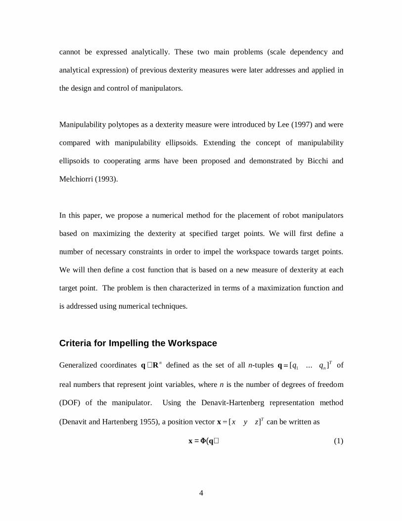
Generalized coordinates q R∈ n defined as the set of all n-tuples q= [ ... ]q qnT

1 of

real numbers that represent joint variables, where n is the number of degrees of freedom

(DOF) of the manipulator. Using the Denavit-Hartenberg representation method

(Denavit and Hartenberg 1955), a position vector x= [ ]x y z T can be written as

x q= F( ) (1)

5

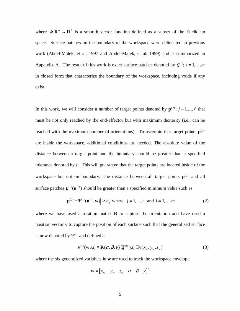
where F:R Rn → 3 is a smooth vector function defined as a subset of the Euclidean

space. Surface patches on the boundary of the workspace were delineated in previous

work (Abdel-Malek, et al. 1997 and Abdel-Malek, et al. 1999) and is summarized in

Appendix A. The result of this work is exact surface patches denoted by x ( ) ; ,...,i i m =1

in closed form that characterize the boundary of the workspace, including voids if any

exist.

In this work, we will consider a number of target points denoted by p( ) ; ,...,j j =1 l that

must be not only reached by the end-effector but with maximum dexterity (i.e., can be

reached with the maximum number of orientations). To ascertain that target points p( )j

are inside the workspace, additional conditions are needed. The absolute value of the

distance between a target point and the boundary should be greater than a specified

tolerance denoted by ε. This will guarantee that the target points are located inside of the

workspace but not on boundary. The distance between all target points p( )j and all

surface patches x ( ) ( )( )i iu should be greater than a specified minimum value such as

p u w( ) ( ) ( )( , )j i ij− ≥Y ε where j =1,...,l and i m=1,..., (2)

where we have used a rotation matrix R to capture the orientation and have used a

position vector v to capture the position of each surface such that the generalized surface

is now denoted by Y( )i and defined as

Y x( ) ( )( , ) ( , , ) ( ) ( , , )i iw w wx y zw u R u v= ⋅ +α β γ (3)

where the six generalized variables in w are used to track the workspace envelope.

w = x y zw w w

Tα β γ

6

and where ε j > 0 are specified constants. If a target point satisfies both conditions of Eq.

(1) and (2), then this point is internal to the workspace (i.e, have placed the workspace in

a configuration such that all points are covered by the workspace).

In order to impel the workspace towards the target points, we propose the following two

constraints: (1) The target points must satisfy the constraint equation (i.e., located in the

workspace volume) and (2) The distance between the target-points and the workspace

must satisfy specified constraints in order for the target points not to be located on the

boundary. These constraints are defined as follows:

(1) Workspace envelope at least covering the target points (shortest distance between

target points):

gii

� - �min ( , )( )p q wG ε for i =1,...,l (4)

where the totality of points in the workspace are also translating and rotation in space

G F( , ) ( , , ) ( ) ( , , )w q R q v= +α β γ x y zw w w

and β is a very small positive number and subject to the inequality constraints on joint

limits as

q q qkL

k kU

� � for k n=1,..., (5)

(2) Embedding the target points inside the workspace volume (a minimum distance

between target points and surface patches).

gkj i

j≡ − ≥p u w( ) ( ) ( , )Y ε for i m=1,..., and

j =1,...,l, k m= �1,..., ( )l (6)

where ε j is the depth of the target point inside the workspace volume. There are

l l+ � +( )m n total number of constraints.

7

Placement of the Manipulator for Maximum Dexterity

In this section, we define a cost function that is based on maximizing the dexterity at

target points. Indeed, to mathematically formulate this problem, it is necessary to use an

analytic dexterity measure at specific target points that can be manipulated. Because

dexterity measures in the literature do not account for joint limits and because of the need

for an analytical expression that can be used in the proposed optimization method, we

define a new dexterity measure.

Dexterity Measure

In serial manipulators, joints are constrained, sometimes due to space limitation, others

strictly by design and are usually specified by an inequality constraint of the form

q q qiL

i iU

� � , where qiL is the lower limit and qi

U is the upper limit. In order to include

joint limits in the formulation, we have used a parameterization to convert inequalities on

qi to equalities q qi i i= ( )λ . Joint limits imposed in terms of inequality constraints in the

form of q q qiL

i iU≤ ≤ , where i n= 1, ... , are transformed into equations by introducing a

new set of generalized coordinates λ = λ λ λ1 2, ,..., n

T such that

q q q q qi iL

iU

iU

iL

i= + + −( ) ( ) sin2 22 7 2 7 λ i n= 1,..., (7)

These generalized coordinates λi are called slack variables in the field of optimization,

where l = ∈λ λ λ1 2, ,..., n

T nR . For any admissible configuration xo and qo , i.e., at a

target in space, the following ( )n + 3 augmented constraint equations must be satisfied

8

G zq x

q q0( )

( )

( )

=

-�!

"$# =

+ �

F

l

o

o n( ) −

3 1

(8)

where the augmented vector of generalized coordinates is z x q= [ ]T T T Tl . By

defining a new vector z q* [ ]=

T T Tl (input parameters), the augmented coordinates can

be partitioned as

z x z=

T T T* (9)

The set defined by G z( )* is the totality of points in the workspace that can be touched by

the end-effector of a serial robot manipulator while considering joint limits. The input

Jacobian of G z( )* is obtained by differentiating G with respect to z* as

G0

I qz

q* =

�!

"$#

F

l

(10)

which is an ( ) ( )n n+ ×3 2 matrix, where Fq = ∂Φ ∂i jq is a ( )3× n matrix, I is the

( )n n× identify matrix, and ql= � �qi jλ is an ( )n n× diagonal matrix with diagonal

elements as q bii i iλ λ) cos= . We define Gz* as the augmented Jacobian matrix.

Since this Jacobian inherently combines information about the position, orientation, and

joint limits of the end-effector, it is a viable measure of dexterity. Furthermore, because

of the simplicity in determining an analytical expression of Gz , it is by far a simpler

approach in comparison with the widely used manipulability ellipsoid. We define the

dexterity measure as

WdT

= G Gz z* * (11)

9

Note that the measure characterized by Eq. (11) takes into consideration all joint limits

and singular orientations.

Geometric Significance of the New Dexterity Measure

1. Relationship with the singular values

A singular value decomposition of the augmented Jacobian matrix can be represented by:

G q U Vz* ( ) * *= 1 1 1S

T (12)

where U R1 ³+ � +( ) ( )m n m n and V R1

2 2³

�n n are orthogonal matrices, and

S1

1

2

0 0 0

0 0 0 0

0 0 0

=

�

!

"

$

####³

+

+ � +

σσ

σ

....

: : .... : :

....

( ) ( )

m n

m n m nR (13)

where σ i i m n, ,...., = +1 are the singular values of Gz* . Substituting Eq.(12) into

Eq.(11) yields

WdT T

= =det( ) det( )* *G Gz z

S S1 1 (14)

where Wd m n=+

σ σ σ1 2* * *L (15)

Equation (15) indicates that the dexterity measure is the product of augmented singular

values. When the augmented Jacobian matrix degenerates, one or more singular values

will be zeros, then the measure is zero, i.e, some of three type singularities occurs.

2. Equivalent Ellipsoid Geometry

From Eq. (10), we have:

δδ

δδ

δ δx

q

qR Qz z

�!

"$# =

�!

"$# = ¼G or G

l* (16)

which is equivalent to

10

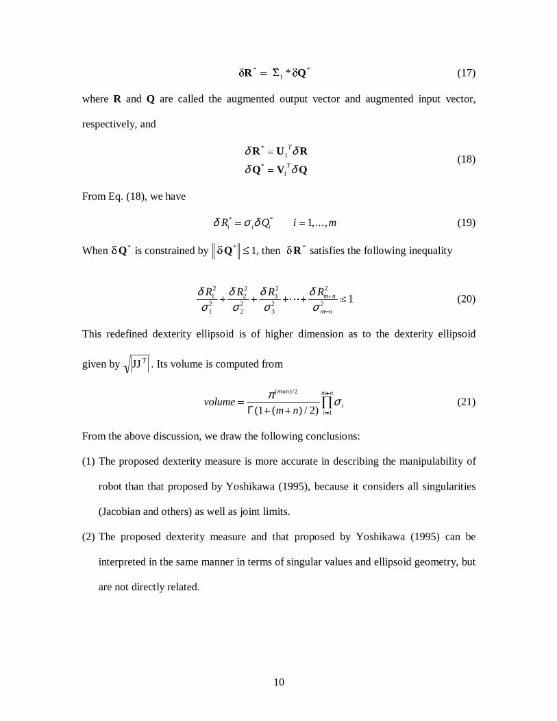
d dR Q* **= S1 (17)

where R and Q are called the augmented output vector and augmented input vector,

respectively, and

δ δδ δ

R U R

Q V Q

*

*

=

=

1

1

T

T(18)

From Eq. (18), we have

δ σ δR Q i mi i i* * ,...,= =1 (19)

When dQ* is constrained by dQ*� 1, then dR * satisfies the following inequality

δσ

δσ

δσ

δσ

R R R Rm n

m n

12

12

22

22

32

32

2

2 1+ + + + �+

+

L (20)

This redefined dexterity ellipsoid is of higher dimension as to the dexterity ellipsoid

given by JJ T . Its volume is computed from

volumem n

m n

ii

m n

=

+ +

+

=

+

ºπ σ

( )/

( ( ) / )

2

11 2Γ(21)

From the above discussion, we draw the following conclusions:

(1) The proposed dexterity measure is more accurate in describing the manipulability of

robot than that proposed by Yoshikawa (1995), because it considers all singularities

(Jacobian and others) as well as joint limits.

(2) The proposed dexterity measure and that proposed by Yoshikawa (1995) can be

interpreted in the same manner in terms of singular values and ellipsoid geometry, but

are not directly related.

11

Mathematical Modeling of the Placement Problem

Given l target points P( ) ( , , )ii i ix y z for i =1 2, , ,L l defined in space, we introduce a

dexterity measure at each point denoted by Wdi( )( )P , where it is necessary to place the

manipulator to achieve maximum dexterity at each target point. Note, however, that this

is a multi-objective optimization problem. Therefore, we will give dexterity at each point

a weight so as to transfer the problem into a usual optimization problem that can be

readily solved.

A mathematical model of the placement of the robot base subject to maximizing the

dexterity at specified target points is characterized by the following optimization

problem.

Cost function

Maximize f Wi di

i

( ) ( , )( )w w p=

=

Êω 1

l

(22)

where ω i i, , , ,= 1 2L l are specified weights at each target point.

Subject to:

(1) Target points are inside the workspace volume (Eq. 2).

(2) Target points are not on the boundary of the workspace envelope (Eq. 4).

(3) The manipulator is constrained

q q qL U� � (23)

(4) The motion is within a finite space

w w wL U� � (24)

12

The set of constraints in Eq. (23) is to impose the unilateral constraints on each joint and

the second set (Eq. 24) to constrain the motion of the base within a finite space.

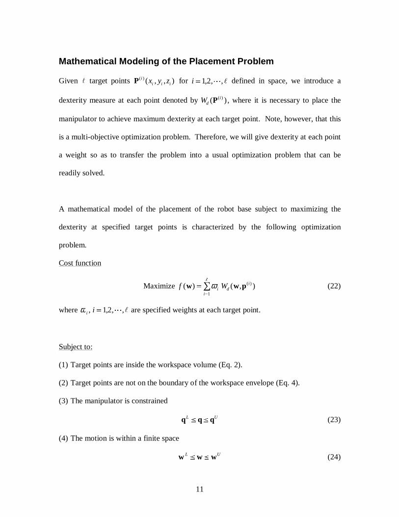
The algorithm for achieving placement is shown in Fig. 1.

Define target points Reach envelope has been identified

Cost functione.g., dexterity

Constraints (no need for inverse kinematics)

Move boundary of workspace

Satisfies Tolerance

Stop

Iterate

w = w + ∆wIterative algorithm to move the workspace

Define robot(dimension and ranges of motion)

Defined by the six generalized coordinates w that characterize its position and orientation

Fig. 1 Algorithm for placement based on optimization

Simple Example

Consider a planar 3DOF manipulator arm as shown in Fig. 2 consisting of 3 revolute

joints. This example will be used to illustrate the theory and will be followed by a more

realistic manipulator model of the upper extremity. There are three target points, namely,

13

T]1014[)1( =P , T]50100125[)2( =P , and T]75125125[)1( =P , which must be

touched by the end-effector with the ability to reach these points from many directions

(i.e., maximizing dexterity).

z3

z0z1z2

421

Fig. 2 Model of the arm with three revolute joints

The coordinates of a point on the end-effector are given by

++++++++++

=Φ)sin()sin(2sin4

)cos()cos(2cos4)(

321211

321211

qqqqqq

qqqqqqq (27)

For simplicity, ranges of motion on each joint are defined as 33 ππ ≤≤− iq ; 3,2,1=i .

The Jacobian is calculated as

Fq =- - + - + + - + - + + - + +

+ + + + + + + + + + +

�!

"$#

4 2 2

4 2 21 1 2 1 2 3 1 2 1 2 3 1 2 3

1 1 2 1 2 3 1 2 1 2 3 1 2 3

sin sin( ) sin( ) sin( ) sin( ) sin( )

cos cos( ) cos( ) cos( ) cos( ) cos( )

q q q q q q q q q q q q q q

q q q q q q q q q q q q q q

Results of the workspace determination yield the following boundary curves (note that

curves are generated because we have restricted the manipulator to planar movement.

The boundary curves are defined by the following sets:

]0 ,3[ );0,,3( 22 ππ −∈qqx , ]3,0[ );0,,3( 22 ππ ∈qqx ,

] 3,3[ );0,0,( 21 ππ−∈qqx ]0,3[ );,3,3( 33 πππ −∈−− qqx

]3,0[ );,3,3( 33 πππ ∈qqx ]3,3[ );3,3,( 11 ππππ −∈−− qqx

and ]3,0[ );3,3,( 11 πππ ∈qqx .

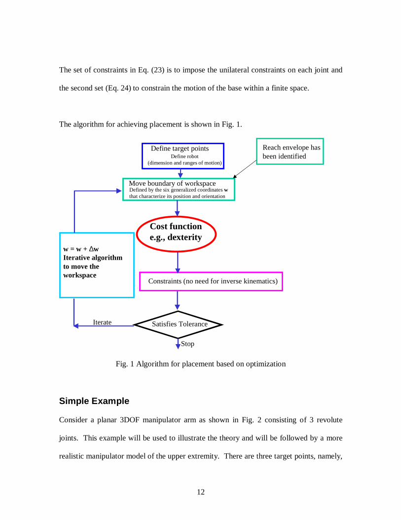
Subsitituting the singular sets into Eq. (27) yields equations of curves shown in Fig. 3,

which is the exact workspace of the planar 3DOF arm (Abdel-Malek and Yeh 1997). We

shall use x and y for positioning and α for orienting the workspace.

14

x

1.0

2.0

3.0

4.0

1.02.03.04.0

y

Fig. 3 The exact workspace of the arm (restricted to planar motion)

As a result of the iterative algorithm, the three design variables representing the position

and orientation of the workspace are calculated as [ ]Tyx α=w

[ ]T674.0663.4714.10= and shown in Fig. 4.

-10 -5 5 10 15 20

-10

-5

5

10

15

20

Fig. 4 The initial and final positions of the arm

15

The measure of dexterity at each point is calculated as

D 80.79)( )1( =P D 040.28)( )2( =P D 914.16)( )3( =P

Note that any configuration that would have included the three points is a solution,

however, the solution calculated using this method yields the position of the arm that

would maximize the dexterity at all three points.

Example: A spatial 3DOF arm

Consider a 3DOF spatial manipulator where the coordinates of end-effector are given by

x q( )

sin cos cos

cos

sin sin sin

=

- +

+

- +

�

!

"

$###

2 5

2

2 5

1 2 2

2 3

2 1 2

q q q

q q

q q q

where joint limits are specified by 0 21� �q π , 0 2� �q p , and 0 83� �q .

The boundaries of the workspace consist of eight surfaces due to the singular sets listed

below. The workspace is shown in Fig. 5.

s( )1 ={q1 3 2= π / , 0 2� �q π , 0 83� �q }s( )2 ={q1 2= π / , 0 2� �q π , 0 83� �q }s( )3 ={p p� �q1 3 2* / , 0 2� �q p , q 3 0= }s( )4 ={p p/ 2 1� �q , 0 2� �q p , q 3 0= }s( )5 ={3 2 21* / *p p� �q , 0 2� �q p , q 3 8= }s( )6 ={0 21� �q p / , 0 2� �q p , q 3 8= }s( )7 ={0 21� �q *p, q 2 0= , 0 83� �q }s( )8 ={0 21� �q *p, q 2 = p , 0 83� �q }

16

-5

0

5

0

5

10

0

2

4

6

-5

0

5

Fig. 5 The workspace of a 3-DOF manipulator

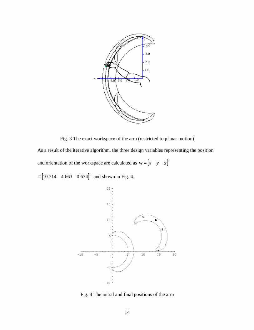
Three target points are specified as p( ) ( , , )1 30 34 33 , p( ) ( , , )2 30 32 37 , and

p( ) ( . , , . )3 334 35 358 . The results of the calculations are listed in Table 2, where initial and

final configurations of the manipulator are shown. The trace of the coordinates of the

origin of the base is plotted in Figure 6. The relative positions of workspaces and work-

point are shown in Figure 7.

Table 2: The original and new base positionParameters x0 y0 z0 a b g

Initial .000 .000 .000 .000 .000 .000Final 34.023 38.594 37.895 1.762 4.342 .380

17

Fig. 6 The trace of the coordinates of the base of the manipulator

Fig. 7 Illustration of results for the placement of the 3DOF manipulator

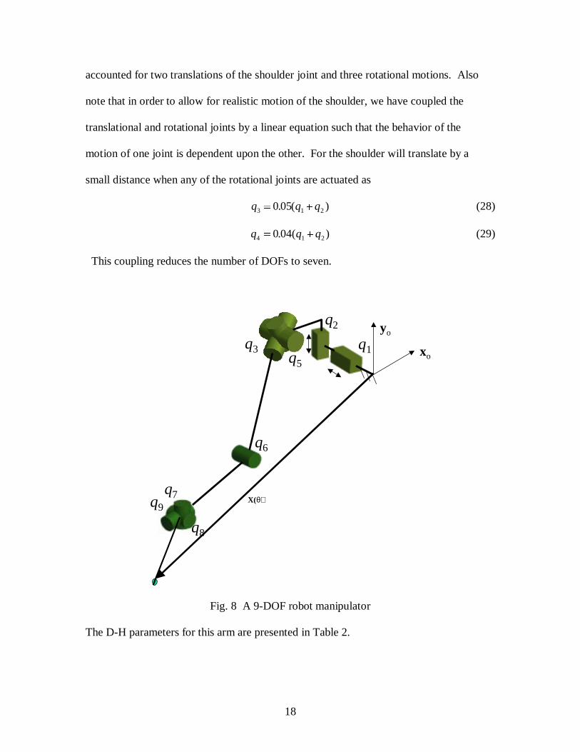
Example: A 9DOF robot manipulator

Consider a model of the upper extremity shown in Fig. 8 and modeled as a total of 9DOF

(5DOF in the shoulder, 1DOF in the elbow, and 3DOF in the wrist). Note that we have

18

accounted for two translations of the shoulder joint and three rotational motions. Also

note that in order to allow for realistic motion of the shoulder, we have coupled the

translational and rotational joints by a linear equation such that the behavior of the

motion of one joint is dependent upon the other. For the shoulder will translate by a

small distance when any of the rotational joints are actuated as

q q q3 1 20 05= +. ( ) (28)

q q q4 1 20 04= +. ( ) (29)

This coupling reduces the number of DOFs to seven.

q1

q2

q3q5

q6

q7

q8

q9

xo

yo

X(θ)

Fig. 8 A 9-DOF robot manipulator

The D-H parameters for this arm are presented in Table 2.

19

Table 2: DH Table for the armθ i di ai α i

1 π 2 q1 0 -π 22 -π 2 q2 0 π 23 0+q3 0 0 π 2

4 π 2+q4 0 0 π 2

5 0+q5 0 20 cm -π 26 0+q6 0 25 cm π 2

7 0+q7 0 0 -π 28 q8-π 2 0 0 -π 29 0+q9 0 0 0

Ranges of motion for this arm are as follows (note that the first two joints are

translational): - � �38 381. .q cm ; - � �38 382. .q cm ; - � �π π2 23q ;

- � �11 8 2 34π πq ; - � �π π2 25q ; 0 5 66� �q π ; - � �π π3 37q ;

- � �π π9 98q ; and - � �π q9 0.

It is required to place the human (as represented by the arm’s workspase) such that the

following three target points are touchable and dexterity is maximized.

T]50100100[)1( =P , T]50100125[)2( =P , and T]75125125[)1( =P .

Note that this is a common problem that arises in the design of assembly lines, cells, and

in any ergonomic design of workplaces.

The position of a point on the end-effector is determined from the Denavit-Hartenberg

formulation as

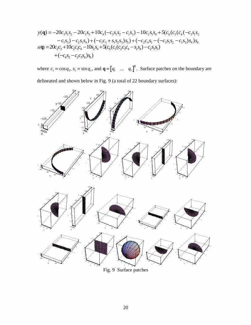
x c c s s s c c c s s s c c s c c c c c s

s s c c s c s c s s s c c c c c s s s s s

( ) ( ) ( ( ( (

) ) ( ) ) ( ( ) )

q =- + + - + - + -

+ - + + + - - +

20 20 10 10 51 3 2 1 3 4 1 3 2 1 3 1 2 4 6 5 4 1 3 2

1 3 1 2 4 3 1 1 2 3 5 1 2 4 1 3 2 1 3 4 6

20

y( ) ( ) ( ( ( (

) ) ( ) ) ( ( ) )

q =- - + - - - + -

- - + - + + - - - -

20 20 10 10 53 1 2 1 3 4 3 1 2 1 3 2 1 4 6 5 4 3 1 2

1 3 2 1 4 1 3 1 2 3 5 2 4 1 3 1 2 1 3 4 6

c s s c s c c s s c s c s s c c c c s s

c s c s s c c s s s s c c s c s s c s s s z c c c c c s s c c c c c s s c s s

c s c c s s

( ) ( ( ( ) )

( ) )

q = + - + - -

+ - -

20 10 10 52 3 2 3 4 2 4 6 5 2 3 4 2 4 2 3 5

4 2 2 3 4 6

where c q1 1= cos , s q1 1= sin , and qT

= q q1 7... . Surface patches on the boundary are

delineated and shown below in Fig. 9 (a total of 22 boundary surfaces):

-4-2024X

-100

-75

-50

-25

0

Y

-4-2024Z

-4-2024X

-100

-75

-50

-25

0

Y

-4-2024X

-50

-25

0

25

50

Y

-60

-40

-20

0

Z

-4-2024X

-50

-25

0

25

50

Y

-4-2024X

-50

-25

0

25

50

Y

0

20

40

60

Z

-4-2024X

-50

-25

0

25

50

Y

0

20

40

60X

-50

-25

0

25

50

Y

-4-2024Z

0

20

40

60X

-60

-40

-20

0X

-50

-25

0

25

50

Y

-4-2024Z

-60

-40

-20

0X

010

2030X

0

25

50

75

100

Y

-20

0

20

Z

010

2030X

0

25

50

75

100

Y

-30-20

-100X

0

25

50

75

100

Y

-20

0

20

Z

-30-20

-100X

0

25

50

75

100

Y

-4-2024X

0

25

50

75

100

Y

-20

0

20

Z

-4-2024X

0

25

50

75

100

Y

010

2030X

0

25

50

75

100

Y

-20

0

20

Z

010

2030X

0

25

50

75

100

Y

-30-20

-100X

0

25

50

75

100

Y

-20

0

20

Z

-30-20

-100X

0

25

50

75

100

Y

-4-2024X

0

25

50

75

100

Y

-20

0

20

Z

-4-2024X

0

25

50

75

100

Y

-20

0

20X 0

25

50

75

100

Y

0

10

20

30

Z

-20

0

20X

-20

0

20X 0

25

50

75

100

Y

-4-2024Z

-20

0

20X

-20

0

20X 0

25

50

75

100

Y

-30

-20

-10

0

Z

-20

0

20X

-20

0

20X 0

25

50

75

100

Y

-4-2024Z

-20

0

20X

-20-10

010

20X

0

25

50

75

100

Y

-20

-10

0

10

20

Z

-20-10

010

20X

0

25

50

75

100

Y

-50-25

0

25

50X

-50

-25

0

2550

Y

-50

-25

0

25

50

Z

-50-25

0

25

50X

-50

-25

0

2550

Y

-20

0

20X 0

25

50

75

100

Y

-30

-20

-10

0

Z

-20

0

20X

-20

0

20X 0

25

50

75

100

Y

0

10

20

30

Z

-20

0

20X

Fig. 9 Surface patches

21

These surface patches are combined, the 7DOF workspace is calculated, and shown in

Fig. 10. Note that we will use the six variables w = x y zw w w

Tα β γ to track

the motion of the workspace envelope.

-40-20

020

40

X

-200

20

Y

-40

-20

0

20

40

Z

-40

-20

0

20

40

Z

-40-2002040

X

-200

20Y

-40

-20

0

20

40

Z

-40-2002040

X

Fig. 10 Workspace of the upper extremity

As a result of the iterative algorithm, the six design variables representing the position

and orientation of the workspace are calculated as

[ ]T736.0463.1850.0171.94444.83235.107 −=w

The measure of dexterity at each point is maximized and its value is

D 83.11687907)( )1( =P D 47.18419793)( )2( =P D 54.13962690)( )3( =P

The initial and final configurations of the workspace of the arm are shown in Fig. 11.

22

Fig. 11 Initial and final configurations of the workspace

Conclusions

A general optimization method for locating the base of a serial manipulator in a work

environment while maximizing dexterity at specified target points was presented. It was

shown that it is possible to place the manipulator by effecting translation and orientation

of the workspace generated in closed form and characterized by surface patches on the

boundary. It was shown that the placement problem can be formulated as an optimization

problem where the cost function is dexterity and the constraints pertain to including the

target points in the workspace.

23

A new dexterity measure was introduced that takes into account singular behavior and

joint limits, which is a fundamental improvement over that reported by Yoshikawa

(1995).

It was shown that the proposed dexterity measure can be used as a cost function in an

optimization algorithm whereby the robot workspace’s motion is tracked using six

generalized variables. The final position and orientation of these variables determine the

placement of the base. The method and code were demonstrated using a simple planar

example and using a spatial model of the upper extremity with 9DOFs.

ReferencesAbdel-Malek, K. and Yeh, H.J., (1997), “Path Trajectory Verification for Robot

Manipulators in a Manufacturing Environment” IMechE Journal of EngineeringManufacture, Vol. 211, part B, pp. 547-556.

Abdel-Malek, K., Adkins, F., Yeh, H.J., and Haug, E.J. (1997), “On the Determination ofBoundaries to Manipulator Workspaces,” Robotics and Computer-IntegratedManufacturing, Vol. 13, No. 1, pp.63-72.

Abdel-Malek, K., Yeh, H-J, and Khairallah, N., (1999), “Workspace, Void, and VolumeDetermination of the General 5DOF Manipulator, Mechanics of Structures andMachines, 27(1), 91-117.

Bergerman, M; Xu, Y, 1997, “Dexterity of underactuated manipulators”, Proceedings ofthe 1997 8th International Conference on Advanced Robotics, ICAR’97 Jul 7-9,1997, Monterey, CA, pp. 719-724.

Bicchi, A.; Melchiorri, C., 1993, “Manipulability measures of cooperating arms”,Proceedings of the 1993 American Control Conference Jun 2-4, IFAC, pp. 321-325.

Denavit, J. and Hartenberg, R.S., (1955), "A Kinematic Notation for Lower-PairMechanisms Based on Matrices", Journal of Applied Mechanics, vol.77, pp.215-221.

Kim, Jin-Oh; Khosla, Pradeep, K., 1991, “Dexterity measures for design and control ofmanipulators”, Proceedings of the IEEE/RSJ International Workshop on IntelligentRobot and Systems ’91, v 2, pp. 758-763.

Lee, J., 1997, “Study on the manipulability measures for robot manipulators”,Proceedings of the 1997 IEEE/RSJ International Conference on Intelligent Robotand Systems. Part 3 (of 3) Sep 7-11 1997 v 3 1997 Grenoble, France, pp. 1458-1465.

24

Pamanes-Garcia, J.A., 1989, “A Criterion for the Optimal Placement of RoboticManipulators”, Proceedings IFAC Information Control Problems in manufacturingTechnology, Madrid, Spain.

Park, F.C.; Brockett, R.W., “Kinematic dexterity of robotic mechanisms”, InternationalJournal of Robotics Research, v 13 n 1 Feb 1994 p 1-15.

Rastegar, J.; Singh, J.R., 1994, “New probabilistic method for the performance evaluationof manipulators”, ASME Journal of Mechanical Design, v 116 n 2, pp. 462-466.

Seraji, H., 1995, “Reachability Analysis for Base Placement in Mobile Manipulators”,Journal of Robotic Systems, Vol. 12(1), pp. 29-43.

Sturges, R.H., 1990, “Quantification of machine dexterity applied to an assembly task”,International Journal of Robotics Research, v 9 n 3 Jun 1990 pp. 49-62.

Wang, J.Y.; Wu, J.K., 1992, “Computational environment for dextrous workspaceanalysis”, DE Advances in Design Automation–Proceedings of 18th Annual DesignAutomation Conference, v 44 pt 2, pp. 293-302.

Yang, F.-C.; Haug, E. J., 1991, “Numerical analysis of the kinematic working capabilityof mechanisms”, DE Advances in Design Automation-Proceedings of 17th DesignAutomation Conference, v 32 pt 1, pp. 9-17.

Yoshiakawa, T., 1985, Manipulability of Robotic Mechanisms”, International Journal ofRobotics Research, Vol. 4(2), pp. 3-9.

Youheng, X; Kaidong, Z, 1993, “Optimum synthesis for workspace dexterity ofmanipulators”, Journal of Shanghai Jiaotong University, v 27 n 4 1993 p 40-48.

Zeghloul, S., Pamanes-Garcia, J.A., 1993, “Multi-criteria optimal placement of robots inconstrained environments”, Robotica, Vol. 11, pp. 105-110.

Appendix A

Using the Denavit-Hartenberg representation, the position of the end-effector can be

analytically formulated as

x q=F( ) (a1)

where q R= ³q q qnn

1 2, ,..., is the vector of joint coordinates. Joint limit constraints are

imposed using the transformation defined in Eq. (7) as q q= ( )l . For any admissible

configuration, the following ( )n + 3 augmented constraint equations must be satisfied

G zq x

q q0( )

( )

( )=

-

-

�!

"$#=

F

l

o

o

(a2)

where the augmented vector z x q=

T T T T, ,λ . Singularity sets resulting from a row-rank

deficiency criteria must be determined to generate envelopes to the workspace. These

25

envelopes are characterized by surface patches that exist inside, outside, and extending

both internal and external to the workspace. The input Jacobian of G q( )* is obtained by

differentiating G with respect to z as

G0

I qz

q* =

�!

"$#

F

l

(a3)

which is an ( ) ( )n n+ ×3 2 matrix, where Fq = ∂Φ ∂i jq is a ( )3× n matrix, I is the

( )n n× identify matrix, and ql= � �qi jλ is an ( )n n× diagonal matrix with diagonal

elements as q bii i iλ λ) cos= , where Gz is defined as the augmented Jacobian matrix.

The objective is to find the constant subvectors of q, denoted by s, which make the sub-

Jacobian Gz row rank deficient. Three singularity types are identified:

(1) Jacobian singularities (called Type I) that satisfy

S ( ) : ] ,1� ³ <s q 3 sq Rank[ for some constant F= B (a4)

(2) A set characterized by a null space criteria imposed on the reduced-order

manipulator (called Type II singular set)

S Null T( ) ; dim [ ( )] ,2 1= ³ �s q q qq for some Φ> C (a5)

where Φq q( ) is the Jacobian after reducing the order of the manipulator.

(3) The set defined by a combination of all constant generalized coordinates (called

Type III singular set)

S q q i j n i jio

jo( ) ;3 1= ³ �s q , for , = to ; > C (a6)

Substituting these singular sets into the position vector defined by Eq. (a1) yields

parametric singular geometric entities (curves or surfaces) defined by

26

x F( ) ( ) ( ) ( )( ) ( )i i i iu u , s� (a7)

Intersections between these singular surfaces may exist. Moreover, these curves partition

a singular surface into a number of regions called subsurfaces. The result is the

identification of all boundary surface patches that characterize the manipulator’s

workspace.