1

Chapter 2

Fundamentals of Image processing

Point transformation

Look up Table (LUT)

2

Introduction (1/2)

• Point to point transformation

• Local to point transformation

3 Types of operations in Image Processing

- m: rows index

- n: column index

Image Processing is based on three types of operations. The first two of these three types are

presented in this figure:

- Point to Point transformation where the pixel value P(m0, n0) of the processed

image « b » is only dependant of the pixel value P(m0’, n0’) of the input image

« a ». Usually, the coordinates (m0’, n0’) are the same at the output and the input:

(m0’, n0’) = (m0, n0);

- Local to Point transformation. The value of one element of image b depends on

pixels taken within a window R(m, n) in image a. This window is usually made

of a limited number of pixels located around pixel (m0’, n0’) in the input image

a: for example a rectangular block of pixels (size K × L), more generally a

specific neighborhood of the pixel (m0’, n0’) conserving the same shape and size

whatever the coordinates (m0’, n0’) are.

3

• Global to point transformation

Characterization of these transformations

Introduction (2/2)

Image size: N x N ; Neighborhood size : p x p ; complexity: in operation per pixel

The last type of transformation is presented in this figure.

- Global to Point transformation. The value of the output at coordinates (m0, n0)

is dependant of all the pixels in the input image a. This is typically the case

when we perform a global transformation of the image into another space.

Discrete Fourier Transform (DFT) or Discrete Cosine Transform (DCT) are

examples of this type where each frequency component X(νX, νY) is a function

of all the pixels of the image to transform.

If we look at the complexity of the processing in terms of number of operations to perform per

pixel at the output, this number is very dependent of the type of processing, from one to N2

(square image (N × N) ), going through P2

for a window size of (P × P) for a local operator

such as linear filtering by convolution.

Another aspect to look at would be more or less regularity in accessing the image data in the

memory of the processor which can slow down the image processing time considerably. It is

only mentioned here.

4

Image

CapturingADC

Image

Memory

ImageDisplaying

DAC

Image

Video output

Processor Bus

Video

Controler

Image

Memory

Image

Processor

Display

Video

Controler

Image

Processor Bus

Image Bus

Video

output

Video

ControlerImage

Memory

Image

Processor

Display

Controler

Digital Image Processing System: typical structures

(a)

(b)

The typical structure of an image processing system is given in this figure. We see at the top a

first (simple) version composed of:

the digitalization of analog video signal (sampling & quantization) into digital image data.

These data can be stored in an image memory at the sampling rate of the video, transmitted to

the second part of the system and/or displayed on a monitor through a DAC;

The image processing is performed by a general purpose processor.

At the bottom, a dedicated image processing unit shows a specific architecture well suited for

processing digital images or successive frames of video. It is composed of a dedicated image

processor able to perform in real-time operations (linear and non-linear as well) on a limited-

size window: (3 × 3) or (5 × 5) window size as well as Point transformation at the input

(before processing) and at the output (before displaying).

5

Pixel operations• no memory operation needed

• map a given gray or color level u of

input signal i to a new level v of

output signal o, i.e. v = f ( u )

• does not provide any new

information

Point Transformation

• point transformation can improve visual

appearance or make targets easier to

detect/extract

Point transformation can be easily performed with digital values. It corresponds to the

transformation of a scalar value into a new one (scalar or vectorial for a color image). It is

fully determined by a characteristic function giving the values at the output for each possible

value at the input. The main effect of the use of point transformation is to modify the

appearance of an image when displaying it immediately after (display of false color image

from a grayscale one) or to modify the gray level or color at the input when we want to

compensate some non-linearity due to the image sensor. Another interesting use will be in the

modification of the image contrast for enhancement purposes.

6

Point Transformation to displayPrinciple (for a grayscale image)

Each pixel of input image Ie, of grayscale Ng, is transformed into T(NG) in the

output image Is through the use of a Look-Up Memory

Objectives

• Display range expansion (contrast enhancement)

• Non-linearity correction

• Image binarization

• Segmentation

The basic principle of a point transformation in a (grayscale) digital image is to consider the

pixel input value as an address and to read the content of the memory at this address. The

content is the transformed value. To do that, original values must have been converted into

non negative integers ranging from 0 to typically 2L –1 (quantization and coding of the gray

level or color pixel components on 2L different values each). For a 8-bit pixel coding the size

of the memory is of 256 bytes.

A color corresponds to each index “i”. This color is created by the combination {ri, gi, bi} of

primary colors Red-Green-Blue. The three values {ri, gi, bi} are sent to three “digital-to-

analog converter (DAC)” to modulate the screen Red-Green-Blue electron guns. By assigning

a different image band to each gun, we can create a false color composite image to aid in

visual interpretation.

This type of memory is called a Look Up Table (LUT) as its content is computed off-line and

not modified during the scanning of all the pixels of the image to transform with the help of

the memory. These small-size dedicated memories can be modified during the video

synchronization slot time (when the video is not displayed on the TV monitor). This is a good

way to realize fading transition between shots in video.

We have usually one LUT at the input and one at the output of a digital image processing

system for grayscale images and two sets of 3 LUT’s for color images (one LUT for each of

the color components RGB).

7

Examples of point transformation

Is

0 Ie255

255

Is

0 Ie255

255 Negative image

Example 1

Example 2

Identity transformation : IS = Ie

gray-level reverse scaling

If you do not want modify the value, you need to use transparent LUT: the content of the

memory at address Ng is Ng. It corresponds to the identity transformation (Example 1). If we

want to realize an inverse video for which a low gray-level value is transformed into a high

gray-level value and vice versa, the content of the LUT at address Ng is (2L - Ng –1).

8

IsB

A

0 a b IMIe

I

Examples of gray-level transformations• Image scaling correction

• Sensor correction

T2 o T1 = Identity operator

Contrast enhancement

Two other examples of gray-level point transformations:

Top figure: all the pixels of the input image Ie with value lower than “a” (respectively higher

than “b”), will get the value “A” (respectively “B”) in the output image IS. The gray-level ue

in image Ie with value included in the range [a, b] will be transformed into a new value vS

between [A, B]. [ ] A)AB(abauv e

s +−−−= .

The goal is to increase the pixel value range [a, b] up to the range [A, B] and to enhance the

contrast. In this case the contrast enhancement factor is worth (B-A) / (b-a).

Bottom figure: shows a typical sensor correction. A cathode ray tube is naturally non linear:

light intensity reproduced on screen is a non-linear function of input tension. Gamma

correction can be considered as a process which allows us to compensate these effects to

obtain a faithful reproduction of the light intensity. Gamma effects are represented by

functions f(x)=xγ, where γ is a real value in the range [2; 2.5] in case of television

applications. Note that the concatenation of the two transformations (where T2 follows T1)

gives an Identity transformation.

9

Piecewise continuous transformations

Example

InterestOne performs two thresholdings :

- Values [0, ...,m[ and ]M,...,255] are kept (the output value is

equal to the input value)

- Pixels into the range [m...M] are set to 255 (« white pixel »)Is

Ie255

255

m M

M

m

Is

Ie255

255

m M

Another transformation :

Other examples:

- Top figure: all the pixels of the input image Ie with values in the range [m, M]

are set to the value 255 (“white”). For other values (higher than M or lower

than m) the input is preserved.

- Bottom figure: the opposite transformation, meaning that only the pixels with

values inside the range [m, M] are kept; the others are reset.

These two point transformations are typical examples of piecewise continuous

transformations.

The bottom figure shows results for the image Barbara. These results are obtained by

piecewise continuous transformations.

Exercise Chapter 2 – Basic tools for image processing - LUT

This exercise is mainly an observation exercise (there are few programming jobs) during

which you will be not only familiarized with the use of Matlab for image processing (which

will help you for the next exercises) but also with the use of basic image processing tools.

Launch Matlab and update the path list in the path browser.

To build a Look-up Table (LUT)

1 – Starting session

From the Matlab command window, open a new file "M-File" in which you will type your

commands and of which each line (finishing with “;”) will be then interpreted.

2 – Open an image

Start by loading the grayscale image CLOWN_LUMI.BMP with imread (take a look at the

Matlab help). Observe the type of the data.

3 – Display and conversion

The image display can be done with the commands image, imagesc et imshow. Observe the

differences; also carry out a test by converting your data (cf. Exercise « Introduction to

Matlab » of chapter 1: try image=double(image)).

4 – Examples of LUT

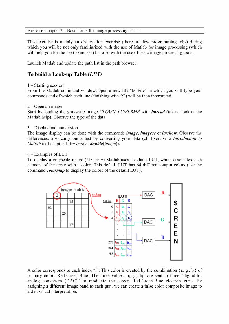
To display a grayscale image (2D array) Matlab uses a default LUT, which associates each

element of the array with a color. This default LUT has 64 different output colors (use the

command colormap to display the colors of the default LUT).

A color corresponds to each index “i”. This color is created by the combination {ri, gi, bi} of

primary colors Red-Green-Blue. The three values {ri, gi, bi} are sent to three “digital-to-

analog converters (DAC)” to modulate the screen Red-Green-Blue electron guns. By

assigning a different image band to each gun, we can create a false color composite image to

aid in visual interpretation.

Matlab allows you to build a specific LUT and to use it with the colormap function.

Colormap must have values in [0,1]. Let us consider, for example, the simple case of a 3 × 3

matrix M:

=

5 3 3

2 2 1

1 5 5

M

This matrix has 4 distinct values. We want to visualize: “1” in black, “2” in white, “3” in red,

and “5” in green. To do this, we build a LUT called “map4C”: the LUT outputs are the 4

required colors. Type the command colormap(map4C) to apply this LUT:

M = [5 5 1;1 2 2;3 3 5] ;

% LUT

r = [0 1 1 0];

g = [0 1 0 1];

b = [0 1 0 0];

map4C = [r’ g’ b’];

image(M)

colormap(map4C)

Results before and after the use of the command colormap( ):

To display an achromatic image in gray levels you must use a LUT so that all output colors

are gray scales: iii bvr ],255 ,0[i ==∈∀ (typically for a 8-bit pixel coding there are 256 gray

levels)

ACTION: Load the script lutndg.m in your working folder. Open and analyze this script.

From this script, visualize your achromatic image in gray levels with the command lutndg.m.

Here are the images before and after using the LUT of the script lutndg.m:

Let us consider another example of LUT creation from Matlab: a screen generates “gamma

effects” which can be compensated (non-linear transformation of the input image gray levels).

To compensate the gamma effects we create a LUT which is the inversion of the gamma

effects so that the concatenation “LUT o gamma effects” is a identity transformation.

Here is an example of a script to compare the images before and after the gamma

compensation:

I = imread(‘CLOWN_LUMI.BMP’);

% LUT to display image clown_lumi in gray levels

r=0:1/255:1;

g=0:1/255:1;

b=0:1/255:1;

map=[r’ g’ b’];

image (I);

colormap(map)

% LUT to compensate gamma effects

vect = 0:1/255:1;

gamma_r = 2.2; % output=input^2.2 (red)

gamma_g = 2.3; % output=input^2.3 (green)

gamma_b = 2.1; % output=input^2.1 (blue)

r = vect.^(1/gamma_r);

g = vect.^(1/gamma_g);

b = vect.^(1/gamma_b);

% we build the LUT with these 3 vectors

map_gamma_inv = [r' g' b'];

% to apply the LUT

figure

image(I)

colormap(map_gamma_inv);

Here are the results before (image on the left) and after (image on the right) using the LUT to

compensate the gamma effects:

ACTION: From the preceding examples, synthesize a LUT to make the video inversion of

the image CLOWN_LUMI. This image processing consists of carrying out the inversion (well-

known in photography) of each color plane i.e. levels 0 become 255 and conversely, levels 1

become 254, etc.

5 – To display the R-G-B components

Load the color image CLOWN in your working folder. Observe the type of the data and

visualize the image. Visualize the color image CLOWN plane by plane by creating adequate

LUTs for the planes Red, Green, and Blue (base this on the exercise “Breaking up a color

image” from chapter 1).

Exercise solution: Look-up Table 1 – Open a script editor using the method of your c hoice (cf. exercise “Matlab initiation”) 2 – In your working folder type the command:

I = imread( ‘CLOWN_LUMI.BMP’); I is a 2D array for a grayscale image. The data typ e of I is uint8 (unsigned integer). 3 – There are three Matlab function for displaying images: imshow, image, and imagesc.

+ imshow displays the image stored in the graphics file or the corresponding matrix. imshow calls imread to read the image from the file, but the image data is not stored in the Matlab work space. The file must be in the current directory or on the MATLAB path.

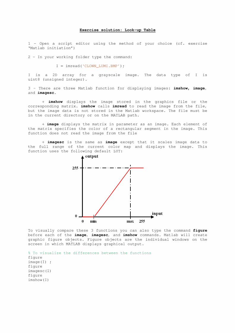
+ image displays the matrix in parameter as an image. Each element of

the matrix specifies the color of a rectangular seg ment in the image. This function does not read the image from the file + imagesc is the same as image except that it scales image data to the full range of the current color map and display s the image. This function uses the following default LUT:

To visually compare these 3 functions you can also type the command figure before each of the image, imagesc, and imshow commands. Matlab will create graphic figure objects. Figure objects are the indi vidual windows on the screen in which MATLAB displays graphical output. % To visualize the differences between the function s figure image(I) ; figure imagesc(I) figure imshow(I)

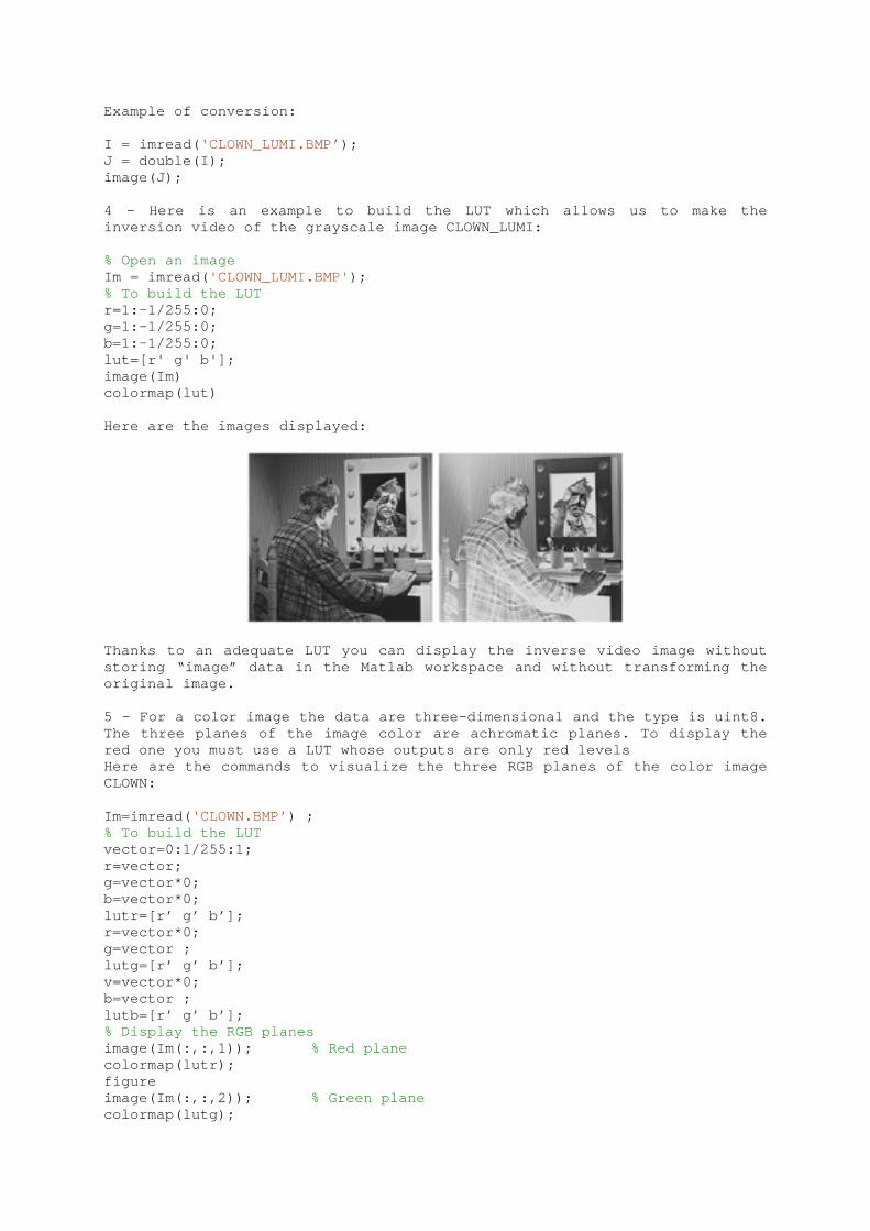
Example of conversion: I = imread( ‘CLOWN_LUMI.BMP’); J = double(I); image(J); 4 – Here is an example to build the LUT which allow s us to make the inversion video of the grayscale image CLOWN_LUMI: % Open an image Im = imread( 'CLOWN_LUMI.BMP'); % To build the LUT r=1:-1/255:0; g=1:-1/255:0; b=1:-1/255:0; lut=[r' g' b']; image(Im) colormap(lut) Here are the images displayed:

Thanks to an adequate LUT you can display the inver se video image without storing “image” data in the Matlab workspace and wi thout transforming the original image. 5 – For a color image the data are three-dimensiona l and the type is uint8. The three planes of the image color are achromatic planes. To display the red one you must use a LUT whose outputs are only r ed levels Here are the commands to visualize the three RGB pl anes of the color image CLOWN: Im=imread( ‘CLOWN.BMP’) ; % To build the LUT vector=0:1/255:1; r=vector; g=vector*0; b=vector*0; lutr=[r’ g’ b’]; r=vector*0; g=vector ; lutg=[r’ g’ b’]; v=vector*0; b=vector ; lutb=[r’ g’ b’]; % Display the RGB planes image(Im(:,:,1)); % Red plane colormap(lutr); figure image(Im(:,:,2)); % Green plane colormap(lutg);

figure image(Im( :, :,3)); % Blue plane colormap(lutb); Here are the images displayed:

Note : Matlab is a matrix visualization tool which propo ses specific LUTs. These LUTs are presented in the “ Supported Colormaps” section of the Matlab help on the colormap. However you cannot build a LU T for color images with Matlab: it is not possible to create a LUT for each color plane Red, Green, Blue.

What is an Histogram ? Example for a gray-level image

Size : 256 ×

256 pixels, 8-bit pixel coding

Distribution of gray levelsin image [0 ; 255]

for each gray level, count the number of pixels having that level for each level, a stick represent the number of pixels(can group nearby levels to form a bin and count number of pixels in it)

8 ×

8 Grayscale image « A »

Matrix of gray levels of image « A »

Histogram of image « A »

2 2 2 2 2 2 2 22 0 0 0 0 0 0 22 0 1 1 1 1 0 23 0 1 0 0 1 0 22 0 1 1 1 1 0 22 0 1 0 0 1 0 22 0 0 0 0 0 0 22 2 2 2 2 2 2 2

There are respectively 24, 12 and 28 pixels for the levels 0, 1and 2

⇒ Histogram of image “A”

Example: compute histogram of an image

Image « A » has 3 different gray levels : 0, 1 and 2.

Count the number of pixels for each gray level.

Image « A » Intensity values of « A » Cumulated histogram of « A »2 2 2 2 2 2 2 2

2 0 0 0 0 0 0 22 0 1 1 1 1 0 22 0 1 0 0 1 0 22 0 1 1 1 1 0 22 0 1 0 0 1 0 22 0 0 0 0 0 0 22 2 2 2 2 2 2 2

Cumulated histogram of an image

compute a special histogram thanks to the cumulative sum of histogram elements ⇒ cumulated histogram.

the cumulated histogram is useful to a lot of image processing such as

hi t li ti ( t t h t)

for each gray level “L”, the stick represents the cumulative sum of pixel

number for all the gray levels lower or equal than L: levels 0, 1, 2 are

thus represented by 24, 36 and 64 pixels.

Exercise Chapter 2 – Computing a histogram

In this exercise you will learn to use the image histogram function imhist which creates and

plots the image histogram. A simple example is introduced in order to understand what is a

histogram. Then you will compare different image histograms (grayscale and color images).

1 – Use the Matlab help (command help or helpwin) to display the description of the Matlab

function imhist.

2 – Create the matrix im1 such as each element im1(i, j), (i, j) ∈ [1, 4]², specifies the gray

level of the pixel (i, j) in the following image:

Use the following values:

- Black pixel intensity = 0 ;

- Gray pixel intensity = 127/255 ;

- White pixel intensity = 1.

Display im1 with the imagesc function and check your coefficients visually (you can build an

adequate LUT to display your image in gray levels. To apply this LUT, use the colormap

function).

Plot the im1 image histogram with the command: imhist(Im1,3). Analyze the result.

3 – Load into your working folder the two grayscale images « FRUIT_LUMI » and

« ISABE_LUMI ». Open these two images with the imread function. Display and compare the

histograms of the two images.

4 – Load and open the color image « MANDRILL ». Use the imhist function and visualize

plane by plane the histograms of the RGB planes for this color image.

Exercise solution: Computing a histogram 1 – The imhist function computes and plots grayscale image histograms. The imhist function can only be used plane by plane for color images. 2 – Here are the commands to plot the histogram of the 4 ×4 image:

im1=[127/255 127/255 0 1;127/255 0 0 1;0 127/255 0 1; 127/255 127/255 0 1] % Build the LUT to display in gray levels r=[0 0.5 1]; g=[0 0.5 1]; b=[0 0.5 1]; map=[r’ g’ b’]; imagesc(im1); colormap(map) ; % Plot the image histogram figure imhist(im1,3) ; Here is the plotted histogram:

The histogram displays the number of pixels for eac h gray level. There are thus 6 black pixels, 6 gray pixels, and 4 white pix els. You can easily visualize this result on the original 4 ×4 image.

3 – Let us read the grayscale images FRUIT_LUMI.BMP and ISABE_LUMI.BMP with the command imread. We can thus build the histograms for these graysc ale images:

I = imread( ‘FRUIT_LUMI.BMP’ ) ; J = imread( ‘ISABE_LUMI.BMP’ ) ; imhist(I); imhist(J);

The two peaks of pixel populations in the FRUIT_LUMI image histogram correspond to the darkest image zones (ground, grap e, etc.) and to the zones which have a middle gray level (intensity clo se to 127 for apples, background, etc.).

Histogram and FRUIT_LUMI image

Here is the histogram of ISABE_LUMI image:

Histogram and ISABE_LUMI image

Here the most important peaks of population corresp ond to the floor shown in the image (the darkest zone) and to the backgrou nd of the image (the lightest zone).

4 – In the case of color images such as MANDRILL.BMP image, we read the image file with the imread function then we compute the histogram plane by plane (there are three achromatic planes: Red, Gree n, and Blue). I = imread( ‘MANDRILL.BMP’ ) ; imhist(I(:,:,1)); % first plane: Red imhist(I(:,:,2)); % second plane: Green imhist(I(:,:,3)); % third plane: Blue

MANDRILL.BMP (first plane: Red) MANDRILL.BMP (second plane: Green)

MANDRILL.BMP (third plane: Blue)

Chapter 2

Fundamentals of Image processing

Histogram transformation

Contrast enhancement by histogram stretching

Max

IsMax

00 a b

I e

Max

Histogram

00 a b

Ie

#

Histogram

stretching

� Histogram stretching:

This first histogram transformation performs an image contrast enhancement. For that, we

must increase on the histogram (top figure) the range [a, b] of gray-level distribution of the

input image Ie. This process is called histogram stretching. A maximum stretching (bottom

figure) is performed so that the gray-level distribution of output image IS occupies the

maximum range [0, Max]. Typically the range [a, b] of Ie will be stretched until the range [0,

255] of IS for an 8-bit pixel coding.

Example of Contrast Stretching

Original image

Stretched image

The bottom figure illustrates a histogram stretching of the image ‘Circuit’. The range of

values for the original image Ie is [12, 182]. After the histogram stretching the gray-level

distribution is displayed on the range [0, 255]. That contains all the gray levels for an 8-bit

pixel coding. The image obtained after stretching has a better contrast. The image contents

relating to electronic structures of circuits are highlighted.

Histogram Equalization

Max

Histogram (original)

00 a b

Ie

#

Max

Histogram

00 a b

Ie

#after equalization

Objective: after transformation,

the histogram becomes constant

Remark : only possible with

continuous data

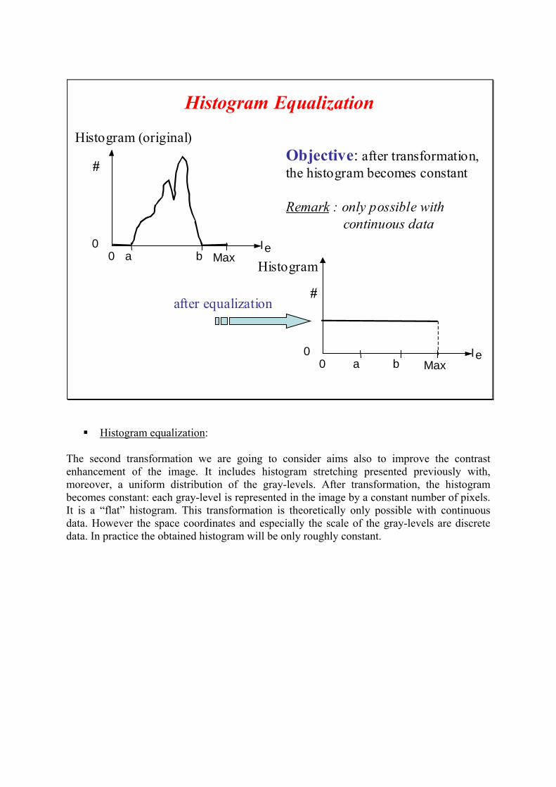
� Histogram equalization:

The second transformation we are going to consider aims also to improve the contrast

enhancement of the image. It includes histogram stretching presented previously with,

moreover, a uniform distribution of the gray-levels. After transformation, the histogram

becomes constant: each gray-level is represented in the image by a constant number of pixels.

It is a “flat” histogram. This transformation is theoretically only possible with continuous

data. However the space coordinates and especially the scale of the gray-levels are discrete

data. In practice the obtained histogram will be only roughly constant.

Digitalization effect on histogram equalization

Observation : if the original image Ie has ‘k’ gray-levels

( k << Max), the output image IS has less than k gray-levels;

Techniques : we define the cumulated histogram of an image Ieas the function CIe on [0, Max], with positive integer values.

Especially CIe(Max) = N

where N is the global number of pixels in the image Ie.

The equalization function f ( i.e. IS = f(Ie) ) is defined by:

f(g) = Max . CIe(g) / N (round integer value)

Especially: f(Max) = Max.

To perform the equalization we use a cumulated histogram. This special histogram inputs for

each gray-level « g » the number of pixels having a gray-level e lower or equal to g. This

number is called )g(C Ie . As “N” is the total number of pixels in the image Ie,N

)g(CIe is thus

the proportion of the pixels having a gray-level lower or equal to g. After equalization the

gray-level “f(g)” will be then the ratio of Max corresponding to this proportion. This fraction

is rounded to the nearest integer.

In this case, after equalization, it is possible to obtain the same gray-level for two initial

different gray-levels g and g': f(g) = f(g '). The number of gray-levels in the image IS can thus

be lower than "k" (k is the number of gray-levels in the original image Ie).

Example of effect of histogram equalization

original image and its histogram image and its histogram after equalization

Visually this first example of equalization enhances the image contrast. The histogram

obtained after equalization is spread out over the entire scale of gray-levels. The discrete data

of the gray-levels does not allow you to obtain a strictly flat histogram.

Contrast enhancement: example and comparison

Original Histogram stretching Equalization

This second example shows the result of a simple histogram stretching and the result of a

histogram equalization. The contrast enhancement is better after the histogram equalization

which more easily detects structures located in the shade.

In fact any strongly represented gray-level is stretched while any weakly represented gray-

level is merged with other close levels.

Exercise Chapter 2 – Histogram transformation

This exercise is mainly an observation exercise. You will use the demonstration imadjdemo

(one of the Matlab image processing demonstrations) to see interactive image processing such

as look-up table transformation, contrast adjustment, histogram equalization, etc.

Contrast Adjustment and Histogram

From the Matlab command window, you must type the command imadjdemo to launch the

demonstration. The following window appears:

You can perform brightness and contrast adjustments, gamma correction and histogram

equalization with the demonstration imadjdemo. The corresponding LUT is plotted and you

can visualize the effects directly on an image and its histogram.

Note : thanks to a LUT, you can change the display without changing the original data.

1 – Start by choosing the image “Circuit”. Change the brightness. Interpret the results.

2 – Modify the contrast and gamma values. Interpret the results. Try to carry out these

modifications on other images than the “Circuit” image and check your interpretations.

Histogram equalization

3 – By using the demonstration imadjdemo, perform a histogram equalization. Visualize the

effects on the image and its histogram.

4 – Use the Matlab help to display the description of the function histeq. Load the grayscale

image CLOWN_LUMI in your working folder then perform the histogram equalization with

the function histeq. Display and compare the images and the histograms before and after the

histogram equalization.

Exercise solution: Histogram Transformation

You will observe how an image is modified when you change some parameters such as the brightness, the contrast, an d the gamma correction. The Matlab demonstration imadjdemo allows you to change these parameters interactively. You can then visualize the differenc es between the original image and the processed image. The demonstration di splays also the image histogram and the LUT, you can thus interpret how t he processed image is obtained.

1 – Here is the image Circuit before and after changing the brightness:

By increasing the brightness value, the LUT is modi fied so that the pixels which had low intensities have now a much more sign ificant intensity. The pixels which have medium and strong intensity value s are set to the maximal output level: 1 (saturation). The stronger the brig htness value is, the more there are pixels with a low intensity which ar e set to 1. You can thus visualize on the histogram (after transformation) a strong number of pixels around the strong intensity values and a peak of po pulation at level 1 due to saturation. The image thus appears “whitened”. B y decreasing the brightness value, the image is “darkened" (inverse phenomena). 2 – By changing the contrast, we visualize the foll owing result:

By increasing the contrast value, the LUT is modifi ed so that the input pixels which have low intensity values are set to t he minimal output level: 0 (saturation). The input pixels which have strong intensity values are conversely set to 1. For the non-saturated pixels, the gray levels are linearly scaled on the full range [0, 1]. The histo gram is stretched and it has two peaks of population: one peak of pixels set to 0 corresponding to the saturation of the pixels which have a low inten sity and one peak of pixels set to 1 corresponding to the saturation of the pixels which have a strong intensity. However the dynamic is linearly f ully used for the other gray levels. The contrast is thus enhanced after st retching (for non-saturated areas). By changing the gamma value, we visualize the follo wing result:

The factor gamma represents the non-linearity of th e light intensity reproduction. A cathode ray tube is naturally non l inear: light intensity reproduced on screen is a non linear function of in put tension. Gamma correction can be considered as a process which all ows us to compensate these effects to obtain a faithful reproduction of the light intensity. Gamma effects are represented by functions f(x)=x γ, where x is the input luminance value and γ is a real value in the range [2; 2.5] in the case of television applications. We must thus build a LUT: g(x)=x 1/ γ to compensate the gamma effects. The pixels which have low intens ities in the original image are then set to stronger intensity values and the dynamic is increased. The details located in the dark areas ar e detected more easily than in the original image: the contrast is enhance d for these dark areas.

3 – Here is the result after having performed the h istogram equalization:

The histogram is almost uniformly stretched on the full range of the gray levels: each gray level is represented in the image by a constant number of pixels. The contrast of the processed image is also enhanced (histogram stretching). 4 – We want to perform the histogram equalization o n any image and without using the demonstration imadjdemo. After having loaded the grayscale image CLOWN_LUMI in your work file, type the following commands to perform a histogram equalization and to display the results: % a LUT to visualize an achromatic image in gray le vels r=0:1/255:1; g=r; b=r; % Histogram equalization I=imread( 'CLOWN_LUMI.BMP') ; image(I) colormap([r' g' b']) figure imhist(I); J=histeq(I); figure image(J) colormap([r' g' b']) figure imhist(J) Here are the obtained images before and after histo gram equalization:

The contrast is definitely more enhanced on the rig ht hand image which is obtained after the histogram equalization. Here are the histograms before (on the left) and af ter (on the right) performing an equalization:

The histogram on the right is almost uniform and a re-scaling is performed ( range = [0, 255] ).

Exercise Chapter 2 – Binarization

This exercise aims to show you different processes to binarize an image (with Matlab). Load

the ISABE_LUMI.BMP image in your file and update the path browser.

1 – Read and display the image (functions imread and image). Display the image histogram

(function imhist) to chose a binary threshold.

2 – With the function im2bw (image processing toolbox) you can convert this grayscale image

to binary by thresholding. Use Matlab help and create and display the binary image of

ISABE_LUMI with the function im2bw.

3 – We want now to create the binary image of ISABE_LUMI without using the function

im2bw. Write a script file for thresholding and binarization. You can use classical Matlab

statements (if, for, etc.) but as Matlab is an interpreter language, it is much more efficient to

work with vectorial data (the function find can be useful).

Exercise solution: Binarization

Binarization is based on a rough thresholding. The output binary image has values of 0 (black) for all pixels in the input image with luminance less than the threshold level and 1 (whit e) for all other pixels. The output image has only two intensity levels (val ue 0 and 1). The output image is a binary image.

1 – After loading the ISABE_LUMI image, enter the f ollowing script: Im=imread( 'ISABE_LUMI.BMP' ); r=0:1/255:1; g=r; b=r; image(Im); colormap([r' g' b']); figure imhist(Im); and we will have the following histogram:

The threshold can be chosen according to different ways. In the case of ISABE_LUMI image, the histogram presents two peaks around the gray levels 75 and 190. We can then for example choose the medi an gray level between these two peaks as threshold. Nevertheless there ar e many other ways to choose the threshold: intensity mean value of the h istogram, median value of the full gray level range [ 0, 255 ])…

2 – We choose the median value 128 of the full rang e [0, 255] as the threshold. This value must be normalized on the ran ge [0, 1] to be used with the function im2bw. The binary image of ISABE_LUMI is then obtained b y the statements: Im=imread( 'ISABE_LUMI.BMP' ); ImBinary=im2bw(Im,128/255) ; imshow(ImBinary); We display the following binary image:

3 – We present 3 other script files to binarize thi s image (threshold=128). a) the first script use “ for ” loops. The goal is to compare each pixel intensity value of the grayscale image to the thres hold:

- if the pixel value (i, j) of the original image i s lower than threshold, pixel (i, j) of binary image is black (v alue 0) ;

- if the pixel value (i, j) of the original image i s higher than

threshold, pixel (i, j) of binary image is white (v alue 1). Here is the Matlab script file to perform this proc ess: threshold = 128; Im = imread ( ‘ISABE_LUMI.BMP’ ); n= size(Im,1); % Number of rows of image m= size(Im,2); % Number of columns of image for i=1:n % each row for j=1:m % each column

if Im(i,j) < threshold ImBinary (i,j) = 0;

else ImBinary (i,j) = 1;

end end end imshow(ImBinary);

b) The second script uses the Matlab function find (to avoid using “ for ” loops and to reduce run time). This function determ ines the indices of array elements that meet a given logical condition. Im=imread( 'ISABE_LUMI.BMP' ); threshold = 128 ; ImBinary=Im; ImBinary (find(ImBinary < threshold))=0; ImBinary (find(ImBinary >= threshold))=1; image(ImBinary) % LUT to display in black and white r=[0 1]; g=r; b=r; map=[r' g' b']; colormap(map); c) The third script also shows the effectiveness of vectorized code with Matlab (you can often speed up the execution of MAT LAB code by replacing for and while loops with vectorized code): Im = imread ( 'ISABE_LUMI.BMP' ); threshold = 128 ; ImBinary = Im > threshold; imshow(ImBinary);

Statement « ImBinary = Im > threshold » creates a logical mask Imbinary which has the same size as Im. One pixel (i, j) of this mask is set to “1” when the condition « Im(i, j) > threshold » is true otherwise it is set to “0”. The mask created is thus the desired binary im age.

Chapter 2 – fundamentals of image processing: point transformation

TEST

1 – Let us consider an input grayscale image Ie, its size is: M rows and N pixels per row.

The associated signal (gray levels) is called se(m, n).

We perform the three following image processes which create:

A) An output grayscale image I1, which is (M × N). The associated signal is called s1(m, n)

and given by: ∑∑+

−=

+

−==

3

3

2

2

1

n

nl

e

m

mk

)l,k(s)n,m(s .

B) An output grayscale image I2, which is (M × N). The associated signal is called s2(m, n)

and given by: s2(m, n) = 128 + [ 255 - se(m, n) ] / 2.

C) An output array A3, which is (M × N). The element a(m, n) is given by:

∑∑==

=N

l

e

M

k

)l,k(s.)l,k(K)n,m(a11

.

Give for each of these three image processes the kind of transformation: global, local, point

to point. Explain your response in one sentence.

2 – Let us consider a digital grayscale image (8-bit pixel coding: gray levels from 0 to 255).

Build the content of a LUT so that:

a ) it makes a video inversion of the gray levels only into the range [a, b] (with a = 88

and b = 148).

b ) all the pixels of the input image with values into the range [a, b] are set to the

black level whereas there is an inverse video effect for all other pixels (a = 88 and b = 148).

c ) it makes it possible to linearize the display on a TV screen. The function which

gives the luminance “L” from the gray levels “gl” is:

L/LMAX = (gl/255)², with LMAX= 70.

3 – Let us consider an achromatic image of a scene. There are only three objects in this scene:

- the background: gray levels into the range [0, a] ;

- an object 1: gray levels into the range [a, b] ;

- an object 2: gray levels into the range [b, 255] ;

with: a = 64 and b = 192.

Build three LUTs which are respectively associated to the three primary colors: Red, Green,

and Blue (LUTR, LUTG, LUTB). We want:

- background pixels displayed in yellow ;

- object 1 pixels displayed in Magenta ;

- object 2 pixels displayed in Cyan ;

For each object the level of luminance does not change. Build the content for each of the three

LUTs and plot it as a function graph (i.e. plot three functions: LUTX=fX(gl) )

4 – Here is the histogram of the grayscale digital image I0:

with: a = 8 ; b = 16 ; c = 24.

We perform a maximal histogram stretching to enhance the contrast. What will be the

maximal stretching factor?

Plot the new histogram obtained with this factor.