polar low over the barents sea: its sensitivity to surface

Original Russian Text © D. A. Iarovaia, V. V. Efimov, 2020, published in MORSKOY GIDROFIZICHESKIY ZHURNAL, Vol. 36, Iss. 3 (2020)

Polar Low over the Barents Sea: Its Sensitivity to Surface Energy Fluxes and Condensational Heating

D. A. Iarovaia*, V. V. Efimov Marine Hydrophysical Institute of RAS, Sevastopol, Russian Federation

* [email protected]

Purpose. The aim of the paper is to study the polar low on January 18–20, 2017 using the sensitivity numerical experiments. The experiments were performed to analyse direct effect of the surface energy fluxes and condensational heating on the cyclone structure and intensity. Methods and Results. The Polar WRF model was used for the cyclone simulations. In order to study the cyclone direct response to the changes in the model, all the experiments started only after the polar low had reached its mature stage at 00:00 on January, 20. Five numerical experiments were performed, in which the following parameters were turned off: 1) sensible heat flux only, 2) latent heat flux only, 3) both surface energy fluxes, 4) phase change heat transfer in the atmosphere and 5) phase change heat transfer in the atmosphere as well as surface energy fluxes. The cyclone intensity was defined by the minimum sea level pressure in its center. Conclusions. It is shown that in all the numerical experiments, the cyclone intensity as well as its maximum wind speed at the model lowest level decreased. In experiments 1 and 2, the intensity decrease was nearly the same, i.e. at the mature stage, the sensible and latent heat fluxes were equally important for the cyclone intensity. In experiments 1, 3 and 5 (with the sensible heat flux turned off), the atmosphere static stability increased significantly due to considerable decrease of the air temperature at the model lowest level. In experiment 4, the planetary boundary layer became more unstable since evaporative cooling was turned off in the model. In experiments 1, 3 and 5, integral kinetic energy of the cyclone increased despite the fact that its intensity and maximum surface wind speed decreased. It is shown that such a response of the cyclone was, most probably, caused by decrease of the energy dissipation in the surface layer due to the increased atmospheric stability.

Keywords: polar low, mesoscale atmospheric modelling, numerical experiments.

Acknowledgments: the investigation was carried out within the framework of project No. 0827-2015-0001 “Fundamental studies of processes in the ocean-atmosphere-lithosphere system which condition spatial-temporal variability of natural environment and climate on global and regional scales”.

For citation: Iarovaia, D.A. and Efimov, V.V., 2020. Polar Low over the Barents Sea: Its Sensitivity to Surface Energy Fluxes and Condensational Heating. Physical Oceanography, [e-journal] 27(3), pp. 225-241. doi:10.22449/1573-160X-2020-3-225-241

DOI: 10.22449/1573-160X-2020-3-225-241

© D. A. Iarovaia, V. V. Efimov, 2020© Physical Oceanography, 2020

Introduction In addition to the usual extratropical cyclones that develop on tropospheric

fronts, small intense cyclones are found in high latitudes above the polar oceans, the occurrence of which is not directly related to tropospheric fronts [1]. Among the set of all polar mesocyclones (PMCs), a separate group of so-called Arctic hurricanes is distinguished. The PMCs of this group reach significant intensity and resemble tropical hurricanes (see, for example, [2, 3]) by external signs (the spiral structure of the cloud system and the presence of an eye), although they may differ from them in the amplification mechanism.

It is known that there is no universal mechanism for the emergence of polar cyclones: PMCs arise due to both baroclinic and convective instabilities, but usually both of these mechanisms act simultaneously, and which one will prevail depends on the specific development conditions [4, p. 403]. According to [4, p. 1; 5], intense

ISSN 1573-160X PHYSICAL OCEANOGRAPHY VOL. 27 ISS. 3 (2020) 225

mailto:[email protected]

PMCs in the North European basin often develop during intrusions of cold Arctic air at sea – therefore, the flux of sensible heat from the sea surface and the release of latent heat during convection can play a significant role in enhancing such PMCs. Therefore, it is always of interest to investigate how exactly the sea-atmosphere interaction affected the intensity of a particular PMC. Note that in the middle latitudes intense mesoscale cyclones resembling tropical hurricanes in their appearance are regularly observed over the Mediterranean Sea [6], one is even observed over the Black Sea [7].

In this paper we will consider the PMC, a distinctive feature of which was an unusually long lifetime – about two and a half days, from January 18 to 20, 2017. This work is a continuation of the previous study devoted to this PMC [8]. In [8], according to the data of ASCAT 1 scatterometer on the near-surface wind, it was found that the cyclone occurred near Iceland, and disappeared in the southern part of the Barents Sea, moving eastward by ~ 2000 km from the place of its origin, i.e. it was not only long-lived, but also mobile – at the mature stage large values of the surface wind velocity (over 30 m/s) were observed in the cyclone. Using the numerical WRF model in [8], the origin and intensification of the cyclone, as well as its trajectory over the Greenland, Norwegian and Barents seas, were reconstructed. It was concluded that PMC intensification was due to the cold air invasion into the Greenland Sea, which began at the end of 18 January and subsequently encompassed the Norwegian and western Barents Sea. According to the simulation results, the strengthening of the cyclone was accompanied by the development of strong convection, while near the surface the convective available potential energy (CAPE) reached large values (more than 1000 J/kg).

In [8], it was not considered what role the large heat fluxes from the sea surface, which arose as a result of cold intrusion, as well as the release of latent heat in convective fluxes, played in the cyclone intensification. We note that in this work we consider in detail the PMC after the onset of the mature stage. The reasons for its origin and the initial stage of cyclone development are not discussed in detail in this work.

PMC description

In this section we briefly describe the polar cyclone development from January 18 to January 20, 2017, using the ERA5 2 reanalysis data with a resolution of 0.25° and 6 h time step. In Fig. 1 the fields of total (sensible + latent) heat flux from the sea surface, sea level pressure and near-surface wind are represented. The cyclone originated at 18:00 on January 18 from a small baric trough to the north of Iceland (–25… –10° E, 66… 70° N) (Fig. 1, a). For 6 hours this area of low pressure shifted ~500 km northeast to the Norwegian Sea (0 ... 10° E, 70 ... 74° N) and closed isobars appeared in it (Fig. 1, b). In the next 6 hours from 00:00 to 06:00 on January 19, a significant increase in the cyclone took place: the pressure in the center abruptly decreased by 16 hPa (Fig. 1, b, c). Obviously, this is explained by the beginning of the cold invasion over the Greenland Sea on January 19, which subsequently spread to the Norwegian Sea (Fig. 1, b, c).

1 Remote Sensing Systems. 2019. Missions List. [on-line] Available at:

http://www.remss.com/missions [Accessed: 10 January 2020]. 2 C3S. 2019. Copernicus Climate Change Service (C3S) ERA5: Fifth generation of ECMWF

atmospheric reanalyses of the global climate, Copernicus Climate Change Service Climate Data Store (CDS). [on-line] Available at: : https://cds.climate.copernicus.eu/ [Accessed: 10 January 2020].

PHYSICAL OCEANOGRAPHY VOL. 27 ISS. 3 (2020) 226

http://www.remss.com/missions

At 06:00 on January 19, the PMC was located between Spitsbergen Island and the coast of Norway, and the total heat flux in the western half of the PMC, which was located above the Norwegian Sea, reached 700–800 W/m2 (Fig. 1, c).

a

b

F i g. 1. Total heat flux, W/m2, sea level pressure, hPa, and sea surface wind, m/s, based on the ERA5 reanalysis data: a – at 18:00 on 18.01.2017; b – at 00:00 19.01.2017; c – a 06:00 on 19.01.2017; d – at 06:00 on 20.01.2917; e – at 18:00 on 20.01.2017. Red line denotes boundary of the area more than a half of which is covered with ice


c

d

e

Continuation of Fig. 1 PHYSICAL OCEANOGRAPHY VOL. 27 ISS. 3 (2020) 228

According to [9], in which the satellite data for 2000–2009 were analyzed, intense PMCs in the North European Basin are observed quite often to the north of the Norwegian coast in 18° E, 72° N region, which is explained by the warm Norwegian current and frequent cold invasions in the Spitsbergen Island area.

For the next 24 hours PMC moved to the northeast, into the Barents Sea, continuing to strengthen, and by 06:00 on January 20 it reached the highest intensity: the pressure in the center dropped to 956 hPa (Fig. 1, d). An additional strengthening of the cyclone was facilitated by the fact that on January 20 the cold invasion distributed to the western half of the Barents Sea (Fig. 1, d, e). After 06:00 on January 20, before reaching the boundary of the ice cover, the cyclone turned to the south and, gradually dissipating, moved towards the coast (Fig. 1, d, e). The next day, January 21, the PMC made landfall and disappeared. As can be seen from Fig. 1, c – e, the cyclone existed in a highly heterogeneous background flux and was not axisymmetric even at the mature stage: the highest surface wind velocity and, accordingly, the highest total heat flux (up to 800 W/m2) were achieved in the western half of the cyclone.

According to the ERA5 reanalysis data, in the development of a cyclone above the sea three stages can be distinguished: a continuous intensification which lasted more than a day (from 18:00 on January 18 to 00:00 on January 20), a mature stage when the cyclone intensity hardly varied (from 00: 00 to 06:00 on January 20), and dissiaption at a constant rate of ~0.4 hPa/h after 06:00 on January 20.

Description of numerical experiments

In order to study the cyclone, we used the polar version of WRF 3.9.1 atmospheric circulation numerical model, well known in the literature [10]. The model used 37 σ-levels unevenly spaced in height with an increased resolution in the planetary boundary layer (the number of levels is indicated for an unstaggered vertical grid). The average height of the levels above the sea in the domain with 2 km resolution was approximately 5.6; 20.7; 39.5; 58.4; 77.3; 96.2; 119; 151; 189; 228; 266; 304; 343; 392; 460; 538; 618; 697; 778; 859; 940; 1022; 1105; 1189; 1274; 1359; 1445; 1531; 1709; 2074; 2679; 3596; 4759; 6109; 7762; 9991 and 1365 m. For parameterization of the planetary boundary layer (PBL), we chose the Yonsei University scheme, in which vK coefficient of vertical turbulent momentum exchange is calculated as

,1κ2

pbl

−⋅⋅=

HzzwKv (1)

where κ is Karman constant equal to 0.4; w is the scale of the vertical velocity in PBL, which is determined through the friction velocity and the sensible heat flux;

pblH is PBL height; z is height [11]. In order to parameterize the surface layer, we used Revised MM5 Monin – Obukhov scheme, in which the friction velocity *u is calculated as


( ) ,/lnκ

01

1* Ψ−

⋅=

zzUu (2)

where 1U – is wind velocity at the lowest model level; 1z is a height of the lowest model level; 0z is roughness length equal to 10-4 m above the sea; Ψ is a universal dimensionless function that depends on the atmosphere stratification [12]. At neutral stratification Ψ = 0, at stable one – Ψ < 0 and at the unstable one – Ψ > 0 [13].

The initial and boundary conditions were taken from the ERA5 operational analysis data with 0.25° spatial resolution and a temporal resolution of 6 hours. The simulation results were output with 1 h step. The simulation was carried out on three nested domains with 18, 6 and 2 km resolutions. 2 km resolution can be considered optimal for modeling a polar mesocyclone, since in [14] an increase in the spatial resolution from 2.2 to 0.5 km when modeling the PMC on March 26, 2013 did not lead to a significant improvement in the results. In Fig. 2 the computational domain in the Barents Sea with 2 km resolution and the cyclone trajectory determined from satellite data, as well as from the results of the control simulation and numerical experiments, is presented. The sea in the domain was completely free of ice. The sea surface temperature during the simulation was kept constant.

F i g. 2. Cyclone trajectory (color lines) based on the results of the control run (0) and numerical experiments (1–5) as well as on the satellite data. Gray color marks out the domain with resolution 2 km. Crosses show location of the cyclone center based on the ASCAT scatterometer data. Numbers by the crosses correspond to the time points: 1 – at 13:36 on 19.01.2017, 2 – at 18:36 on 19.01.2017, 3 – at 11:36 on 20.01.2017 and 4 – at 18:18 on 20.01.2017

To study the role of heat fluxes from the sea surface and the release of latent heat during convection in the intensification of a particular cyclone, numerical sensitivity experiments are carried out – this is a generally accepted practice [15–18]. However, disabling certain physical processes in the model affects not only the cyclone itself but also the entire atmosphere in the computational domain,


which, in its turn, also leads to the changes in the cyclone. According to [18], in the case when the numerical experiment lasts more than a day, it becomes difficult to determine exactly how the disabling of the considered physical process affected the intensity of the cyclone – directly or indirectly, through a change in the environment. In this regard, in [16–18] it is proposed to start the experiment not at the moment of cyclone occurence, but after it reaches a mature stage.

In our case, according to the simulation results, the mature stage of the cyclone began at 00:00 on January 20. Therefore, numerical experiments were carried out according to the following scheme: from 06:00 on January 19 to 00:00 on January 20 – simulation with initial and boundary conditions from ERA5 reanalysis; from 00:00 to 21:00 on January 20 – a numerical experiment with boundary conditions from ERA5 reanalysis and the initial conditions taken from the previous calculation. Due to computational difficulties, the domains could not be made large enough. At the beginning of the calculation, the cyclone is outside the domain with 2 km resolution, but by 00:00 on January 20, moving eastward, it completely enters the domain through its western boundary. After 21:00 on January 20, the cyclone leaves the domain through its southern boundary (Fig. 2). In the future, when analyzing the control simulation, the period from 13:00 on January 19 to 21:00 on January 20 will be considered, since at this time the center of the cyclone was within the domain.

We denote the control simulation as 0 and give a brief description of the experiments, mentioning what was changed in the model:

1. Only sensible heat flux is turned off. 2. Only the latent heat flux is turned off. 3. Sensible and latent heat fluxes from the sea surface are turned off. 4. Heat release/absorption is disabled during phase transitions in the atmosphere. 5. Heat release/absorption during phase transitions in the atmosphere and

fluxes of sensible and latent heat from the sea surface are disabled. All other parameters of the model were left unchanged in the experiments. Unlike a tropical hurricane, sensible and latent heat fluxes in the PMC are

comparable in magnitude, so it is of interest to see how it reacts to the disabling of each of these fluxes separately (experiments 1 and 2). In experiment 5 we disabled both cyclone amplification factors, which were turned off separately in experiments 3 and 4. All experiments lasted 21 hours.

For analyzing the cyclone structure, we used a cylindrical coordinate system, the center of which coincided with the cyclone center and moved with it, as well as the angle-averaged velocity and temperature fields were considered.

Results of experiments

As can be seen from Fig. 2, the trajectory of the cyclone in numerical experiments does not differ from the control simulation. Both in the experiments and in the control simulation, the cyclone at the end of January 19 – beginning of January 20 changes its movement direction in the Barents Sea from northeastern to southeastern, which is consistent with the ASCAT satellite data.

Cyclone intensity Now we consider how the cyclone intensity changed in the experiments in

comparison with the control simulation. The depth of a polar cyclone is usually PHYSICAL OCEANOGRAPHY VOL. 27 ISS. 3 (2020) 231

used as a measure of its intensity, i.e the pressure at the sea level at the cyclone center minslp [18, 19]. Fig. 3, a indicates how minslp value changed with time in the control simulation and in numerical experiments. The experiments began at 00:00 on January 20, when the pressure in the cyclone center in the control simulation dropped to the lowest value – 955 hPa. As expected, in all experiments the cyclone decays faster than in the control simulation. The lowest intensity variation was observed in the experiments 1 and 2 (the deviation from the control simulation does not exceed ~ 3 hPa), more noticeable changes occurred in experiments 3 and 4 (deviation up to 5 hPa). The greatest decrease in intensity, i.e. the highest decay rate, is observed in experiment 5 (the deviation reaches 7 hPa at the end of the calculation).

a b

F i g. 3. Sea level pressure in the cyclone center, hPa (а); maximum tangential speed in the cyclone, m/s, at the model low level (0 – control simulation; 1–5 – numerical experiments)

During the first 6 hours the graphs 1, 2 and 3 in Fig. 3, a do not almost differ

from the graph 0, while in experiments 4 and 5 the decrease in intensity is noticeable already at the beginning of the calculation. That is, the PMC reacted faster to the disabling of heat exchange in the atmosphere due to evaporation/condensation than to the disabling of heat fluxes from the sea surface. This can be explained as follows: as was mentioned above, the experiments began at a mature stage when convection in the cyclone was already well developed, and turning off the air heating from the underlying surface could not lead to an immediate termination of convection.

The graphs 1 and 2 almost coincide, which means that at the considered stage of the PMC development (from the mature stage to disappearance), the fluxes of sensible and latent heat were equally important for maintaining its intensity. We note that such a reaction is not always observed in a polar cyclone. For example, in [18], in which the PMC was studied on December 18–21, 2002, it was shown that after the onset of the mature stage it was the sensible heat flux that was more important.

In order to assess the intensity of the cyclone, the maximum near-surface (at the lower level of the model) wind velocity in the cyclone max_tV is also used (Fig. 3, b). As can be seen from Fig. 3, b, in the experiments the values of max_tV


are generally lower than in the control simulation, and the most noticeable decrease occurred in experiments 1, 3, and 5, in which the sensible heat flux was disabled. Unlike minslp , max_tV sharply decreases already at the very beginning of experiments 1, 3 and 5 and represents the direct reaction of the cyclone to the changes in the model. However, as will be shown below, from Fig. 3, b it does not yet follow that in experiments 1, 3, and 5 a decrease in the cyclone kinetic energy took place.

Thermal structure of a cyclone Now we consider how the temperature field in the cyclone has changed.

In Fig. 4 for 01:00 and 11:00 on January 20, which corresponds to the beginning and the middle of the experiment, the difference between the average potential temperature over the cyclone area in the control simulation and in the experiment (∆θ) is shown. When averaging over the area, the cyclone radius was assumed to be 200 km.

a b

F i g. 4. Deviation of the air potential temperature (averaged over the cyclone area) in the experiments from that in the control simulation, K: a – at 01:00 on January 20, 2017; b – at 11:00 on January 20, 2017 (0 – control simulation; 1–5 – numerical experiments)

As expected, after disabling the sensible heat flux from the sea surface in experiments 1, 3, and 5, the air temperature near the surface decreased. Over the time, the deviation of temperature near the surface from the control run increases and, 11 h after the start of the simulation, reaches 4, 7, and 8 K, respectively (Fig. 4). The effect of sensible heat flux shf on the temperature in the lower atmosphere layer can be assessed from the ratio

pbl,

ρp

shfC H⋅ ⋅

where pC is

specific heat capacity of air at constant pressure; ρ is the air density. We find that a heat flux of 230 W/m2 (Table 1) for 1 h will lead to an increase in the potential temperature in the 1 km layer by 0.8 K. This approximately corresponds to the temperature decrease in the experiment 1 (Fig. 4, a).


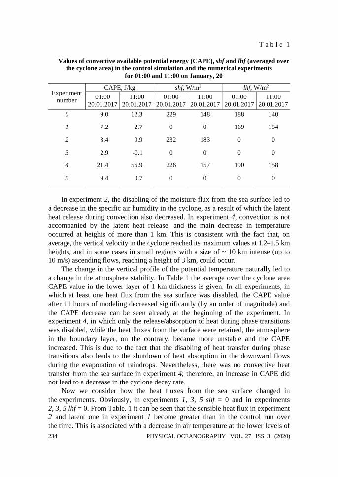
T a b l e 1

Values of convective available potential energy (CAPE), shf and lhf (averaged over the cyclone area) in the control simulation and the numerical experiments

for 01:00 and 11:00 on January, 20

Experiment number

CAPE, J/kg shf, W/m2 lhf, W/m2 01:00

20.01.2017 11:00

20.01.2017 01:00

20.01.2017 11:00

20.01.2017 01:00

20.01.2017 11:00

20.01.2017 0 9.0 12.3 229 148 188 140

1 7.2 2.7 0 0 169 154

2 3.4 0.9 232 183 0 0

3 2.9 -0.1 0 0 0 0

4 21.4 56.9 226 157 190 158

5 9.4 0.7 0 0 0 0

In experiment 2, the disabling of the moisture flux from the sea surface led to

a decrease in the specific air humidity in the cyclone, as a result of which the latent heat release during convection also decreased. In experiment 4, convection is not accompanied by the latent heat release, and the main decrease in temperature occurred at heights of more than 1 km. This is consistent with the fact that, on average, the vertical velocity in the cyclone reached its maximum values at 1.2–1.5 km heights, and in some cases in small regions with a size of ~ 10 km intense (up to 10 m/s) ascending flows, reaching a height of 3 km, could occur.

The change in the vertical profile of the potential temperature naturally led to a change in the atmosphere stability. In Table 1 the average over the cyclone area CAPE value in the lower layer of 1 km thickness is given. In all experiments, in which at least one heat flux from the sea surface was disabled, the CAPE value after 11 hours of modeling decreased significantly (by an order of magnitude) and the CAPE decrease can be seen already at the beginning of the experiment. In experiment 4, in which only the release/absorption of heat during phase transitions was disabled, while the heat fluxes from the surface were retained, the atmosphere in the boundary layer, on the contrary, became more unstable and the CAPE increased. This is due to the fact that the disabling of heat transfer during phase transitions also leads to the shutdown of heat absorption in the downward flows during the evaporation of raindrops. Nevertheless, there was no convective heat transfer from the sea surface in experiment 4; therefore, an increase in CAPE did not lead to a decrease in the cyclone decay rate.

Now we consider how the heat fluxes from the sea surface changed in the experiments. Obviously, in experiments 1, 3, 5 shf = 0 and in experiments 2, 3, 5 lhf = 0. From Table. 1 it can be seen that the sensible heat flux in experiment 2 and latent one in experiment 1 become greater than in the control run over the time. This is associated with a decrease in air temperature at the lower levels of


the model and, as a consequence, an increase in the sea – atmosphere temperature difference, as well as a decrease in the surface air moisture content. As is obvious from Table. 1, in all calculations heat fluxes decreased with time, which is consistent with Fig. 3: in all calculations the cyclone decayed, although at different rates.

Dynamic structure of a cyclone Now we consider how the increase in atmospheric stability affected

the cyclone as a whole. For this purpose, we use such a characteristic as integral

kinetic energy of cyclone rotation E, equal to ∫ ∫=H

S

t dsdzVE0

2

2, where H and S are

the height and area of the cyclone; tV is tangential velocity. The height of the cyclone, i.e. the height of the level at which closed isobars are still traced, does not differ from the control simulation in experiments and is ~ 7 km. The value E, although it is the energy characteristic of the cyclone as a whole, is not used to assess its intensity, in contrast to the value max_tV , since, firstly, it is difficult to

measure, and secondly, max_tV value is of greater practical importance. When calculating the E value, we use only the tangential velocity, since the integral kinetic energy of a cyclone is in fact the kinetic energy of its primary circulation (air rotation in a horizontal plane around the cyclone center). The kinetic energy of the secondary circulation (air inflow to the center of the cyclone at the lower levels, ascent and outflow at the upper levels) is significantly smaller. In our case, the integral kinetic energy of secondary circulation is two orders of magnitude less than the primary one.

F i g. 5. Integral kinetic energy of the cyclone, 1016 m5/s2, in control simulation (0) and numerical experiments (1–5)


As can be seen from Fig. 5, in which the variation with time of E value is shown, the integral kinetic energy of the cyclone in experiments 1, 3, and 5 is greater than in the control run throughout the simulation. Taking into account Fig. 3, b, a seemingly paradoxical result is obtained – the disabling of sensible heat inflow from the sea surface led not only to a decrease in the cyclone intensity and wind velocity near the surface (which is intuitively clear), but also to an increase in its integral kinetic energy. This is especially evident in experiment 3, for which the velocity max_tV decreased by 5–6 m/s (see Fig. 3, b) and the excess of E reached 2·1016 m5/s2.

F i g. 6. Cyclone fields (averaged over the angle in the cylindrical coordinate system) at 11:00 on January, 20: a – in control run; b – in experiment 1; c – in experiment 3; d – in experiment 5 (color shows tangential speed, m/s; black lines – isosters, K; violet isolines – radial speed, m/s). For better visualization, only negative radial speed is shown


Let us illustrate the changes in the cyclone structure described above using Fig. 6, which compares the fields of potential temperature, as well as radial and tangential wind velocities, in the control simulation and experiments 1, 3, and 5. In Fig. 6 it can be seen that in a thin layer near the surface (<100 m) the velocity tV in the experiments decreased in comparison with the control run – this is consistent with Fig. 3, b. However, at the same time the velocity tV in the experiments at 0.3–0.6 km heights, on the contrary, increased, which caused an increase in the integral kinetic energy (see Fig. 5). In addition, the increase in the atmosphere stability, which was discussed in the previous section, led to a decrease in the boundary layer thickness. According to the simulation results, the average over the cyclone area PBL height for the time point shown in Fig. 6 is 910 m in the control simulation and 510, 230, and 270 m for experiments 1, 3, and 5, respectively. A decrease in the PBL height in the experiments led, due to the continuity equation, to an increase in the velocity of radial air flux entering the cyclone at the lower levels. The changes in the cyclone velocity fields described above appeared at the beginning of experiments 1, 3 and 5 and persisted until 18:00 on January 20 when the cyclone began to disappear.

Let us now consider the most probable cause for the increase in the integral kinetic energy of the cyclone. From relations (1) and (2) it follows that the intensity of vertical turbulent exchange in the model depends on the atmosphere stratification. Now we are to find ε – the rate of the cyclone integral kinetic energy decrease due to the work of turbulent friction force. Taking into account that the velocity tV vanishes at the surface and at the cyclone upper boundary, ε value

can be calculated as ∫ ∫

∂∂

=H

z S

tv dsdz

zVK

0

2

ε . As is known, in the surface layer we

apply the logarithmic law of horizontal wind velocity variation with height

=

0

* lnκ z

zuVt , and vertical turbulent exchange coefficient vK increases linearly

with height zuKv ⋅⋅= κ* [20]. Above the surface layer the values of vK coefficient are calculated in the Yonsei University boundary layer parameterization scheme (see expression (1)). Hence we get

.lnκ1ε

1

23*

0

1 ∫ ∫∫

∂∂

+

=

H

z S

tv

S

dsdzz

VKdsuzz (3)

The first term in formula (3), 1ε , takes into account the energy dissipation in the surface layer, i.e. it considers the effect of underlying surface, and the second term, 2ε , – in the overlying layers. Table 2 gives the time-averaged values of 1ε and 2ε for 6:00–11:00 period on January 20, when the rate of integral kinetic energy decrease was almost constant both in the control run and in experiments (see Fig. 5). Also in Table 2 ΔE/Δt value for this period is given. As can be seen from Table 2, after disabling the sensible heat flux, the energy dissipation in the surface layer decreased, while in the overlying layers it, on the contrary,


increased. The first circumstance is due to the fact that the atmosphere stability near the surface has increased significantly. The second circumstance is that the vertical wind shear in the boundary layer has increased (see Fig. 6). From Table 2 it is obvious that, despite the increase in 2ε value, the total rate of energy dissipation, 21 εε + , in all experiments decreased in comparison with the control run due to 1ε value decrease. This is in qualitative agreement with the abovementioned effect.

As can be seen from Table 2, the rate of ΔE/Δt decrease is 1.5–2 times less than it could be expected based on the dissipation value ε. Apparently, this is due to the fact that at the mature stage PMC existed in a heterogeneous background flux with cyclonic vorticity (see Fig. 1, c – e), which arose around a synoptic depression centered in the Barents Sea (50° E, 74° N) and maintained high wind velocities in the western part of the cyclone, where the assessment of the rotation velocity could be overestimated due to the contribution of the background flux velocity.

T a b l e 2

Friction-resulted losses in the control run and numerical experiments 1, 3 and 5

for 6:00–11:00 on January, 20

Experiment number ΔE/Δt, 1011 m5/s3 ε1, 1011 m5/s3 ε2, 1011 m5/s3 0 −8.0 13.7 1.3

1 −6.7 12.5 1.5

3 −5.1 8.2 4.3

5 −5.1 8.7 3.3

Conclusion

Numerical sensitivity experiments were carried out for the PMC, which arose in the Greenland Sea, to the north of Iceland, on January 18, 2017 and moved to the Barents Sea in two and a half days where it reached the highest intensity. The experiments began when it reached a mature stage, at 00:00 on January 20, which made it possible to isolate the direct reaction of the cyclone to the disabling of one or another physical process in the model.

It is shown that the cyclone intensity (the minimum pressure at sea level in the center), as well as the maximum wind velocity near the surface, directly depended on the heat fluxes from the sea surface and the release of latent heat in the upstreams. It was found that at the mature stage sensible and latent heat fluxes were equally important for maintaining the cyclone intensity. In addition, the fact that the cyclone responds to the disabling of latent heat release more rapidly than to the disabling of heat fluxes from the sea surface was found out.

It is shown that disabling at least one of two heat fluxes from the sea surface significantly affects the temperature and velocity fields in the cyclone. At the lower levels the atmosphere becomes more stable, and the thickness of the air radial


inflow at the lower levels decreases. As a consequence, the radial velocity in the boundary layer, directed towards the cyclone center, increases. When only heat exchange due to phase transitions is disabled (experiment 4), the atmosphere becomes more unstable than in the control simulation. This is due to the fact that at the model lower levels the evaporation of raindrops is no longer accompanied by heat absorption.

An interesting cyclone reaction to the disabling of sensible heat flux was revealed: in those experiments in which shf = 0, the integral kinetic energy of the cyclone increases due to an increase in the tangential velocity in the middle part of PBL, although the intensity and maximum tangential velocity at the lower level of the model decrease. The most probable cause of such a cyclone reaction was considered, and it was shown that integral kinetic energy increase in the experiments is due to a lower cyclone decay rate, which corresponds to a lower energy dissipation rate in the surface layer. A drop in the CAPE of the atmosphere in experiments 1, 3, and 5 led to a decrese of friction velocity and the coefficients of vertical turbulent exchange in the model. Thus, in experiments with disabling the sensible heat flux, a complete restructuring of the entire boundary layer, tangential and radial velocity fields took place. We emphasize once again that the sensible heat flux was disabled only after the cyclone intensification occurred, and the increase in atmospheric stability affected the decrease rate of already accumulated kinetic energy of the cyclone but it was not an energy source.

REFERENCES

1. Rojo, M., Claud, C., Mallet, P.-E., Noer, G., Carleton, A.M. and Vicomte, M., 2015. Polar Low Tracks over the Nordic Seas: A 14-Winter Climatic Analysis. Tellus A: Dynamic Meteorology and Oceanography, 67(1), 24660. doi:10.3402/tellusa.v67.24660

2. Emanuel, K.A. and Rotunno, R., 1989. Polar Lows as Arctic Hurricanes. Tellus A: Dynamic Meteorology and Oceanography, 41(1), pp. 1-17. https://doi.org/10.3402/tellusa.v41i1.11817

3. Nordeng, T.E. and Rasmussen, E.A., 1992. A Most Beautiful Polar Low. A Case Study of a Polar Low Development in the Bear Island Region. Tellus A: Dynamic Meteorology and Oceanography, 44(2), pp. 81-99. doi:10.3402/tellusa.v44i2.14947

4. Rasmussen, E. and Turner, J., eds., 2003. Polar Lows: Mesoscale Weather Systems in the Polar Regions. Cambridge: Cambridge University Press, 612 p. doi:10.1017/CBO9780511524974

5. Kolstad, E.W., 2015. Extreme Small-Scale Wind Episodes over the Barents Sea: When, Where and Why? Climate Dynamics, 45(7-8), pp. 2137-2150. https://doi.org/10.1007/s00382-014-2462-4

6. Miglietta, M.M., Laviola, S., Malvaldi, A., Conte, D., Levizzani, V. and Price, C., 2013. Analysis of Tropical-Like Cyclones over the Mediterranean Sea through a Combined Modeling and Satellite Approach. Geophysical Research Letters, 40(10), pp. 2400-2405. https://doi.org/10.1002/grl.50432

7. Yarovaya, D.A., Efimov, V.V., Shokurov, M.V., Stanichnyi, S.V. and Barabanov, V.S., 2008. A Quasitropical Cyclone over the Black Sea: Observations and Numerical Simulation. Physical Oceanography, 18(3), pp. 154-167. https://doi.org/10.1007/s11110-008-9018-2


8. Efimov, V.V., Yarovaya, D.A. and Komarovskaya, О.I., 2020. Mesoscale Polar Cyclone from Satellite Data and Results of Numerical Simulation. Sovremennye Problemy Distantsionnogo Zondirovaniya Zemli iz Kosmosa, 17(1), pp. 223-233. doi:10.21046/2070-7401-2020-17-1-223-233

9. Noer, G., Saetra, Ø., Lien, T. and Gusdal, Y., 2011. A Climatological Study of Polar Lows in the Nordic Seas. Quarterly Journal of the Royal Meteorological Society, 137(660), pp. 1762-1772. doi:10.1002/qj.846

10. Skamarock, W.C., Klemp, J.B., Dudhia, J., Gill, D.O., Barker, D.M., Duda, M.G., Huang, X.-Y., Wang, W. and Powers, J.G., 2008. A Description of the Advanced Research WRF Version 3. Boulder, Colorado: National Center for Atmospheric Research USA, 113 p. Available at: https://opensky.ucar.edu/islandora/object/technotes%3A500/datastream/PDF/view [Accessed: 08 April 2020].

11. Hong, S., Noh, Y. and Dudhia, J., 2006. A New Vertical Diffusion Package with an Explicit Treatment of Entrainment Processes. Monthly Weather Review, 134(9), pp. 2318-2341. https://doi.org/10.1175/MWR3199.1

12. Shin, H.H., Hong, S. and Dudhia, J., 2012. Impacts of the Lowest Model Level Height on the Performance of Planetary Boundary Layer Parameterizations. Monthly Weather Review, 140(2), pp. 664-682. https://doi.org/10.1175/MWR-D-11-00027.1

13. Jiménez, P.A., Dudhia, J., González-Rouco, J.F., Navarro, J., Montávez, J.P. and García-Bustamante, E., 2012. A Revised Scheme for the WRF Surface Layer Formulation. Monthly Weather Review, 140(3), pp. 898-918. https://doi.org/10.1175/MWR-D-11-00056.1

14. Sergeev, D.E., Renfrew, I.A., Spengler, T. and Dorling, S.R., 2017. Structure of a Shear-Line Polar Low. Quarterly Journal of the Royal Meteorological Society, 143(702), pp. 12-26. https://doi.org/10.1002/qj.2911

15. Bresch, J.F., Reed, R.J. and Albright, M.D., 1997. A Polar-Low Development over the Bering Sea: Analysis, Numerical Simulation, and Sensitivity Experiments. Monthly Weather Review, 125(12), pp. 3109-3130. https://doi.org/10.1175/1520-0493(1997)125<3109:APLDOT>2.0.CO;2

16. Yanase, W., Fu, G., Niino, H. and Kato, T., 2004. A Polar Low over the Japan Sea on 21 January 1997. Part II: A Numerical Study. Monthly Weather Review, 132(7), pp. 1552-1574. https://doi.org/10.1175/1520-0493(2004)132%3C1552:APLOTJ%3E2.0.CO;2

17. Føre, I., Kristjánsson, J.E., Kolstad, E.W., Bracegirdle, T.J., Saetra, Ø. and Røsting, B., 2012. A ‘Hurricane-Like’ Polar Low Fuelled by Sensible Heat Flux: High-Resolution Numerical Simulations. Quarterly Journal of the Royal Meteorological Society, 138(666), pp. 1308-1324. doi:10.1002/qj.1876

18. Føre, I. and Nordeng, T.E., 2012. A Polar Low Observed over the Norwegian Sea on 3–4 March 2008: High-Resolution Numerical Experiments. Quarterly Journal of the Royal Meteorological Society, 138(669), pp. 1983-1998. doi:10.1002/qj.1930

19. Michel, C., Terpstra, A. and Spengler, T., 2018. Polar Mesoscale Cyclone Climatology for the Nordic Seas Based on ERA-Interim. Journal of Climate, 31(6), pp. 2511-2532. doi:10.1175/JCLI-D-16-0890.1

20. Holton, J.R., 2004. An Introduction to Dynamic Meteorology. New York, N.Y., USA: Academic Press, 535 p.


About the authors: Daria A. Iarovaia, Senior Research Associate, Marine Hydrophysical Institute of RAS (2

Каpitanskaya Str., Sevastopol, 299011, Russian Federation), Ph. D. (Phys.-Math.), [email protected]

Vladimir V. Efimov, Head of Ocean and Atmosphere Interaction Department, Marine Hydrophysical Institute of RAS (2 Каpitanskaya Str., Sevastopol, 299011, Russian Federation), Dr. Sci. (Phys.-Math.), Professor, ResearcherID: P-2063-2017, Scopus Author ID: 6602381894, [email protected]

Contribution of the co-authors: Daria A. Iarovaia – numerical experiments, processing and interpretation of modeling results,

preparation of figures Vladimir V. Efimov – statement of the problem, participation in the formation of conclusions,

discussion of the results, critical analysis of the text The authors have read and approved the final manuscript. The authors declare that they have no conflict of interest.


polar low over the barents sea: its sensitivity to surface

Documents