pore-scale modeling of hydromechanical coupled mechanics ... fracturing.pdf · pore-scale modeling...

$: Pore-scale modeling of hydromechanical coupled mechanics ... fracturing.pdf · Pore-scale modeling of hydromechanical coupled mechanics in hydrofracturing process Zhiqiang Chen1 and$
Pore-scale modeling of hydromechanical coupledmechanics in hydrofracturing processZhiqiang Chen1 and Moran Wang1

1Department of Engineering Mechanics and CNMM, Tsinghua University, Beijing, China

Abstract Hydrofracturing is an important technique in petroleum industry to stimulate well production.Yet the mechanism of induced fracture growth is still not fully understood, which results in someunsatisfactory wells even with hydrofracturing treatments. In this work we establish a more accuratenumerical framework for hydromechanical coupling, where the solid deformation and fracturing aremodeled by discrete element method and the fluid flow is simulated directly by lattice Boltzmann methodat pore scale. After validations, hydrofracturing is simulated with consideration on the strengthheterogeneity effects on fracture geometry and microfailure mechanism. A modified topological index isproposed to quantify the complexity of fracture geometry. The results show that strength heterogeneityhas a significant influence on hydrofracturing. In heterogeneous samples, the fracturing behavior iscrack nucleation around the tip of fracture and connection of it to the main fracture, which is usuallyaccompanied by shear failure. However, in homogeneous ones the fracture growth is achieved bythe continuous expansion of the crack, where the tensile failure often dominates. It is the fracturingbehavior that makes the fracture geometry in heterogeneous samples much more complex than thatin homogeneous ones. In addition, higher pore pressure leads to more shear failure events for bothheterogeneous and homogeneous samples.

Plain Language Summary Hydrofracturing is an important technique in petroleum industry tostimulate well production. Yet the mechanism of induced fracture growth is still not fully understood,which results in some unsatisfactory wells even with hydrofracturing treatments. This problem may not besolved in continuum scale so that we establish a pore-scale numerical framework to reproduce and simulatethis process. The results show that the failure patterns in hydrofracturing are quite different from those innormal fracturing by pressure. The shear failure plays a very important role besides the tensile failure. Thestrength heterogeneity has a significant influence on hydrofracturing. A quantitative characterization ofheterogeneity and fracture is proposed in this work. Predictions by this method agree well with existingexperimental data for several cases. The results will improve understanding of mechanism of hydrofracturingmechanics and therefore help to optimize the hydrofracturing process in applications.

1. Introduction

Hydraulic fracturing is one of the primary engineering techniques to improve well productivity especially forunconventional energy reservoirs [Economides and Nolte, 2000]. In this process, fluid is pumped into the well,and artificial fracture is induced in the formation by high fluid pressure [Veatch and Moschovidis, 1986].However, as a routine operation to stimulate reservoirs, besides many successes there still exist some wellswhich productions are unsatisfactory even with hydrofracturing [Qiu et al., 2013; Rahman and Rahman,2010; Zhou et al., 2014]. The main reason for this lack of predictability is that the mechanics of crack initiationand propagation during hydraulic fracturing is still not completely understood [Gou et al., 2015; Wanget al., 2014].

In the past few decades, a large number of numerical analysis techniques have been applied to study hydrau-lic fracturing and try to understand its underlying physics [Adachi et al., 2007; Barbati et al., 2016; Detournay,2016]. However, how to develop an accurate and comprehensive numerical model is still a challengingresearch topic [Adachi et al., 2007], although it is of great importance for both hydromechanical coupledtheory and hydrofracturing practice. This complexity arises from two aspects, complex geologic reality(heterogeneity and anisotropy, etc.) and inherent coupled multiphysics process [Economides and Nolte,2000], including solid deformation, fracture propagation, fluid flow in fracture/matrix, and their exchange[Kovalyshen, 2010].

CHEN AND WANG MECHANICS IN HYDROFRACTURING 1

PUBLICATIONSJournal of Geophysical Research: Solid Earth

RESEARCH ARTICLE10.1002/2017JB013989

Key Points:• Pore-scale modeling for hydraulicfracture mechanism of heterogeneousrocks

• Fracture growth patterns are clarifiedby modeling

• Quantitative description of strengthheterogeneity and fracture network isproposed

Correspondence to:M. Wang,[email protected]

Citation:Chen, Z., andM. Wang (2017), Pore-scalemodeling of hydromechanical coupledmechanics in hydrofracturing process,J. Geophys. Res. Solid Earth, 122,doi:10.1002/2017JB013989.

Received 14 JAN 2017Accepted 13 APR 2017Accepted article online 20 APR 2017

©2017. American Geophysical Union.All Rights Reserved.

http://orcid.org/0000-0002-0112-5150

http://publications.agu.org/journals/

http://onlinelibrary.wiley.com/journal/10.1002/(ISSN)2169-9356

http://dx.doi.org/10.1002/2017JB013989

http://dx.doi.org/10.1002/2017JB013989

mailto:[email protected]

Generally, there are mainly two kinds of models for hydrofracturing simulation, continuum-based modelsand discontinuum-based models. In continuum-based models, the governing equations based on conti-nuum theory (including elasticity equation, fluid flow equation, and fracture growth equation) are solvedanalytically or numerically [Adachi et al., 2007]. It began with simplified theoretical models in 1950s suchas KGD and PKN model [Geertsma and De Klerk, 1969; Nordgren, 1972]. After that some variations of KGDand PKN model were developed [Yew and Weng, 2014], including pseudo-3D (P3D) model, a semianalyticalmodel, planar 3-D (PL3D) models, and fully 3-D models [Zhou and Hou, 2013] where the fracture propaga-tion and fluid flow in fracture were solved numerically in 2-D or 3-D meshes, respectively [Adachiet al., 2007].

Although the above continuum-based models are routinely applied in the design of hydrofracturing treat-ment [Zhou and Hou, 2013], they are phenomenological and without detailed attention to the fundamentallyphysical significance [Thallak et al., 1991]. In addition, some predictions by the continuum-based model arenot consistent with the results obtained from the experiment [Al-Busaidi et al., 2005]. First, various types offracture geometry are measured with microseismic mapping ranging from single planar fracture to complexfracture network, and only complex fracture network is desirable in “supertight” reservoirs [Mayerhofer et al.,2010]. However, the complexity of the fracture geometry is difficult to be predicted by the continuum-basedmodel owing to its single planar fracture assumption [Wang et al., 2014]. Second, the continuum-basedmodel generally assumes that the failure mode in hydraulic fracturing is the tensile failure, but shear-typeseismic events are often recorded in experiments and even in some cases shear failure dominates the fractur-ing behavior [Falls et al., 1992; Ishida et al., 2004].

As an alternative, discontinuum-based models based on discrete element method (DEM) were developed toexplore what happened in hydrofracturing at microscale [Al-Busaidi et al., 2005; Bruno et al., 2001; Lisjak et al.,2015; Sheng et al., 2015]. In DEM, the rock is regarded as an assembly of bonded particles, which capturesthe discrete nature of rock effectively and allows for an explicit simulation of the crack nucleation and coa-lescence. In order to solve the fluid flow in rock, different fluid dynamics modeling methods have beenapplied to combine hydromechanical coupled models with DEM. The first type of models is coarse gridmethods [Furtney et al., 2013], where the continuum flow is calculated by solving the Darcy’s law [Brunoet al., 2001] or average NS equations [Eshiet et al., 2013] on the grid larger than the DEM particle. Due tothe inconsistent scale for fluid and solid phase in coarse grid methods, empirical formulas are alwaysneeded. Another popular type is DEM/pore network coupled model, which has been used to study hydro-fracturing recently and achieved some success [Al-Busaidi et al., 2005; Hazzard et al., 2002; Shimizu et al.,2011]. With simplifications of solid structure (pore and throat) and fluid flow (Poiseuille equation),DEM/pore network model can provide fluid field information at particle scale. However, when the rockbreaks up seriously or the void geometry changes dramatically, it is quite difficult to distinguish pore andthroat from the DEM structure [Furtney et al., 2013] and the assumption of a same pore pressure value inthe fracture is not valid anymore [Ni et al., 2015]. Thus, Ni et al. [2015] simulated hydraulic fracturing witha more accurate pore-scale DEM-CFD coupled model, but it is computationally expensive due to remeshingat each time step.

In the past three decades, the lattice Boltzmann method (LBM) has gained much popularity owing to its effi-ciency in dealing with complex boundary. Recently, it has been coupled with DEM to study hydromechanicalproblems in geophysics such as sand production [Boutt et al., 2011; Chen et al., 2016]. In LBM-DEM model,fluid flow and fluid-solid interaction are simulated directly and efficiently at pore scale without adjustableparameters [Boutt et al., 2011]. However, only a few LBM-DEM models are applied to simulate hydraulic frac-turing, although it is necessary to reveal the mechanism involved.

Strength heterogeneity is a common feature in nature rock owing to the preexisting weak joints, cracks,or flaws, which greatly affects the fracture processes and macromechanical properties [Ma et al., 2014,2011; Tang et al., 2000], but the role of strength heterogeneity in hydraulic fracturing process has notbeen fully explored especially quantitatively. In this work, LBM and DEM are coupled to simulate hydrau-lic fracturing at pore scale, and the effects of strength heterogeneity on fracture complexity and micro-failure mechanism are investigated. We try to bridge the gap with a more accurate coupled model,which may help us understand the conflict of failure mode between continuum model prediction andexperimental data.

Journal of Geophysical Research: Solid Earth 10.1002/2017JB013989


2. Numerical Methodsand Validations

This section gives a brief intro-duction of numerical methodsused in current simulation includ-ing lattice Boltzmann method(LBM), discrete element method(DEM), and the LBM-DEM cou-pling method immersed movingboundary (IMB). Then the LBM-DEM coupled scheme is validatedby sphere sedimentation cases.

2.1. Lattice BoltzmannMethod (LBM)

Lattice Boltzmann method (LBM) isan efficient numerical method to

simulate fluid flow, heat, and mass transfer especially with complicated boundary condition and multiphaseinterfaces [Wang et al., 2007, 2016; Zhang and Wang, 2015]. Recently, LBM has been also widely used to simu-late fluid-solid coupling system owing to its high accuracy and efficiency [Boutt et al., 2011; Chen et al., 2013,2015, 2016].

In LBM, the Boltzmann equation is solved in the discrete lattices, and the obtained macroscopic parameters(velocity, pressure, etc.) obey the desired governing equations (such as NS equations) by the Chapman-Enskog expansion [Succi, 2001]. A widespread LBM implementation is the lattice Bhatnagar-Gross-Krookmodel, where the collision operator is simplified as a linearized version [Chen and Doolen, 1998] and theevolution equation is written as

f i x þ eiδt; t þ δtð Þ ¼ f i x; tð Þ � 1τ

f i x; tð Þ � f eqi x; tð Þ� �; i ¼ 0� 14; (1)

where x denotes the position vector, fi is the density distribution in the ith lattice discrete velocity direction ei,f eqi is the corresponding equilibrium distribution, δt is the time step, and τ is the dimensionless relaxation timerelated to the fluid kinematic viscosity

ν ¼ τ � 1=2ð Þδ2x3δt

; (2)

where δx is the lattice size. In current simulation, a three-dimensional 15-speed model (D3Q15) is applied,which is one of standard and representative models for three-dimensional flows [Qian et al., 1992; Wangand Chen, 2007]. “D3” indicates three dimension in space, and “Q15” means that the density distributionhas 15 discrete velocity directions (see Figure 1). In the D3Q15 model, the discrete velocities are

e ¼ c

0 1 0 �1 0 0 0 1 1 1 1 �1 �1 �1 �1

0 0 0 0 0 �1 1 �1 �1 1 1 �1 �1 1 1

0 0 1 0 �1 0 0 1 �1 �1 1 1 �1 �1 1

264

375; (3)

where c= δx/δt. The equilibrium distribution for D3Q15 model is given as

f eqi ρ;uð Þ ¼ ρωi 1þ 3ei � uc2

þ 9 ei � uð Þ22c4

� 3u � u2c2

" #; (4)

Figure 1. The lattice direction system for D3Q15 model.



where the weighting factors are

ωi ¼2=9; i ¼ 0

1=9; i ¼ 1� 6

1=72; i ¼ 7� 14

8><>: : (5)

After evolution, the macroscopic density and velocity can be calculated by

ρ ¼Xi

f i; (6)

ρu ¼Xi

f iei; (7)

and the pressure (p) is given by [Chen and Doolen, 1998]

p ¼ 13ρc2: (8)

2.2. Discrete Element Method (DEM)

Discrete element method (DEM) was proposed in 1979 [Cundall and Strack, 1979] and has achieved great suc-cess in simulating dynamic behavior of brittle material such as rock. In order to overcome the shape limitationof round particles, the spheropolyhedra method is used in current simulation, where the rock is regarded asan assembly of angular particles [Galindo-Torres et al., 2012], and the current DEM algorithm is based on theMechSys open source library.

To model bonding, cohesive forces are assumed at the common face shared by two adjacent particles, whichare given by

Fcohen ¼ Mcohen Aεnn

Fcohet ¼ Mcohet Aεtt

(; (9)

where Fcohen and Fcohet are cohesive forces in normal and tangential directions respectively, A the shared facearea, Mcohe

n and Mcohet the normal and tangential elastic modulus of assumed “bond” material, εn and εt the

normal and tangential strains of two adjacent particle faces, n and t the unit vectors in normal and tangentialdirections. When the relative displacements of two adjacent faces reach the threshold value εth

εnj j þ εtj jεth

> 1; (10)

the bond will be broken and a small crack forms. In this simulation, the broken bonds are classified as shearfailure (εt> εn) and tensile failure (εt< εn), similar to the classification in Shimizu et al. [2011].

Besides cohesive forces, another kind of interaction forces are contact forces caused by particle collisions,which are modeled by the normal and shear spring [Cundall and Strack, 1979]. Normal Fcontn and tangential

Fcontt contact forces are proportional to the overlapping lengths in respective directions

Fcontn ¼ KnΔlnn

Fcontt ¼ KtΔltt

(; (11)

where Kn and Kt are normal and tangential spring stiffness, Δln and Δlt the overlapping lengths in normal andtangential directions, n and t same as that in equation (9). When Fcontt > μfricF

contn ; the tangential force



becomesFcontt ¼ μfricFcontn t;where μfric the particle friction coefficient and Fcontt and Fcontn are the magnitude of

vector Fcontt and Fcontn . More detail about spheropolyhedra method for DEM simulation can be found inGalindo-Torres et al. [2012].

2.3. LBM-DEM Coupling Scheme

For hydromechanical coupled model, two aspects must be considered. First, the no-slip boundary conditionshould be satisfied at the fluid-solid interface. Second, hydrodynamic force applied to solid phase need becalculated owing to fluid-solid interaction. In current LBM-DEM model, the immersed moving boundary(IMB) [Noble and Torczynski, 1998] is used to deal with fluid-solid interaction, which offers resolution at thesubgrid scale and allows for accurate and stable calculation of hydrodynamic force [Strack and Cook, 2007].In IMB, the volume fraction occupied by solid in each cell, namely γ whose value is within [0,1], is obtained,

and a fluid-solid interaction term, ΩSi , is introduced in the evolution equation

f i x þ eiδt; t þ δtð Þ ¼ f i x; tð Þ � 1� Bð Þ 1τ

f i x; tð Þ � f eqi x; tð Þ� �þ BΩsi : (12)

The fluid-solid interaction term ΩSi is derived by the bounce-back for nonequilibrium part

Ωsi ¼ f�i x; tð Þ � f eq�i ρ; vp

� �� f i x; tð Þ � f eqi ρ; vp� ��

; (13)

where vp is the solid velocity at position x. In equation (12), B is a weight function depending on γ in each cell

B ¼ γ τ � 0:5ð Þ1� γð Þ þ τ � 0:5ð Þ : (14)

When γ = 0, B = 0, and γ = 1, B = 1. It means that the evolution equation (equation (12)) can recover the stan-dard LB equation and bounce-back rule for γ = 0 and 1, respectively.

The hydrodynamic force exerted on the DEM particle is calculated by the change of momentum in all cellscovered by the particle

F ¼ δ3xδt

Xn

BnXi

Ωsi ei

!; (15)

where n is the number of cells covered by the DEM particle. The torque T can be calculated similarly

T ¼ δ3xδt

Xn

xn � xcmð ÞBnXi

Ωsi ei

!" #; (16)

where xn is the cell position, and xcm is the mass center of the DEM particle.

2.4. Validations

To validate the current LBM-DEM scheme for fluid-solid coupling problems, two benchmark cases areconsidered, single-sphere sedimentation and two-sphere sedimentation. Because results of direct numericalsimulations for sphere sedimentations have been presented in many previous papers using finite elementmethod (FEM) or other methods [Chen et al., 2015; Glowinski et al., 2001; Sharma and Patankar, 2005; Strackand Cook, 2007], there is sufficient data available for validation.2.4.1. Single-Sphere SedimentationFor a single offset sphere settling down in a column of fluid, it will oscillate around the centerline of the col-umn with decreasing amplitude [Strack and Cook, 2007]. Eventually, a fixed settling velocity is achieved withno lateral motion. Based on this velocity, the terminal particle Reynolds number is calculated

Re ¼ udν; (17)

where u is sphere terminal velocity, d is the sphere diameter, and ν is the kinematic viscosity.



For comparison, the channel andsphere geometry are set as the sameas that in Strack and Cook [2007]. Asphere with diameter d is placed ina square channel L× L wide and 16 Ldeep (L= 3/2d). The initial sphereposition is 0.4 L from the side of col-umn in x direction (see Figure 2a).By adjusting the value of gravity, dif-ferent terminal particle Reynolds canbe achieved. In this case Re = 15, thesphere trajectories obtained by pre-sent LBM-DEMmodel agree well withthat in Strack and Cook [2007].2.4.2. Two-Sphere SedimentationWhen two separated spheres settledown at zero initial velocity (seeFigure 3), a famous phenomenon so-called “drafting, kissing, and tum-

bling” or DKT motion will occur [Fortes et al., 1987]. “Drafting” in this process means the trailing sphere willaccelerate due to the low pressure in the wake of the leading one. Then it catches the leading sphere, and“kissing” motion happens. Owing to the instability of contacting spheres aligned in the settling direction,they tend to “tumble” to another position. As a result, the relative position of two spheres exchanges andthe initial trailing sphere becomes the leading one.

We also simulate this process for further validation, where two spheres with density 1.14 g/cm3 and radius0.083 cm settle down under gravity in a column with square cross section 1 cm × 1 cm and 4 cm depth(see Figure 3a). The centers of two spheres are located at (0.5 cm, 0.5 cm, and 3.4 cm) and (0.5 cm, 0.5 cm,and 3.16 cm) initially. The fluid kinematic viscosity is 0.01 m2/s, and density is 1 g/cm3. The same case wasalso modeled in Glowinski et al. [2001] using FEM and Sharma and Patankar [2005] with finite volumemethod (FVM).

Figure 3b shows the vertical positions of two spheres during the sedimentation process, and up to the kissingstage, our results agree well with that in Glowinski et al. [2001] and Sharma and Patankar [2005]. After the kis-sing stage, exact agreement is not expected, because the “tumbling” is the realization of an instability, anddifferent particle collision models will lead to different motions after kissing [Glowinski et al., 2001; Sharmaand Patankar, 2005].

Figure 2. (a) The geometry of single-sphere sedimentation benchmark case,where a sphere (d = 2/3L) is placed in 0.4L from the side of column in xdirection. (b) The trajectory of sphere in current simulation agrees well withthat in Strack and Cook [2007].

Figure 3. (a) The geometry of two spheres sedimentation benchmark case, where two spheres with radius 0.083 cm settledown under gravity in a square channel with cross section 1 cm × 1 cm and depth 4 cm. (b) The vertical positions oftwo spheres during sedimentation process obtained from different simulations, and our results agree well with others.



3. Hydrofracturing Simulation3.1. Physical Model and Modeling Parameters

The rock sample in current hydrofracturing simulation is presented in Figure 4a, where a hole is set at themiddle of the left edge for fluid injection. For hydrofracturing simulation, the rock sample is first discretizedas an assembly of triangular solid particles (see Figure 4c). To simulate the flow behavior in the rock, the tri-angular particles in Figure 4c are eroded by a small distance to obtain the “flow channel” (see Figure 4d),which is a common numerical approach to deal with fluid-solid coupling process [Boutt et al., 2011;Shimizu et al., 2011]. In Figure 4d, the triangular particle is regarded as impermeable, and the fluid can onlyflow along the triangular grain boundary, namely flow channel, which provides the primary permeabilityfor the rock matrix just like Boutt et al. [2011] for sand production simulation. This idealization can be thoughtof two triangular particles in Figure 4d being separated by a virtual bond beam, which supports particle inter-action force and is permeable to fluid. Current model is a pseudo-2D model for the sake of simplicity andcomputation time, and only one layer of particles is considered, but it can be extended to fully 3-D casewithout difficulty.3.1.1. Fracture Dependent Flow ConductivityFor fluid flow in deforming fractured rocks, an important character is the fracture-controlled fluid flow[Latham et al., 2013; Nick et al., 2011; Yardley, 1983; Zhang et al., 2002], which means new formed cracksare much more permeable than the matrix primary permeability. If a connected fracture is formed, it willdominate the flow behavior in the rock [Zhang et al., 2002]. Thus, the crack propagation and the fluid flowis a strong two-way coupling process. However, previous LBM-DEM schemes did not consider this effect,and when the bond was broken, the flow conductivity did not change at all.

In order to capture this feature, immersed moving boundary (IMB) is also introduced in the flow channel.When the bond is intact, an initial volume fraction (γ < 1) is set for the LBM cells in the flow channel, whichmeans the flow channel is partly occupied by the virtual stationary solid, corresponding to a low flow conduc-tivity. By changing the initial value of γ, different rockmatrix permeability can be achieved, and larger γ resultsin lower rock primary permeability. During the hydrofracturing simulation, the γ of LBM cells in smaller trian-gular particles (see Figure 4d) is updated at each time step by calculating the volume fraction occupied by

Figure 4. Physical model and computational system for simulations. (a) The rock sample used for hydrofracturing simula-tion, where a hole is set in the middle part of left edge for fluid injection. (b) Discretization of rock sample by triangularparticles with same thickness in DEM. (c) The 2-D projection diagram from thickness direction. (d) Two-triangular DEMparticles are bonded together by virtual bond beam, which serves as the flow channel for fluid.



solid. The γ of LBM cells in the flow channel keeps the initial constant value as long as the bond is intact. Whenthe bond is broken (new crack forming), γ in the corresponding flow channel is set to 0, which means flowresistance caused by virtual stationary solid is removed by the formation of crack. As a result, the flowconductivity enhanced by fracture can be captured effectively.3.1.2. Characterization of Strength HeterogeneityStrength heterogeneity is a common feature in rock material and can be quantitatively evaluated by Weibulldistribution [McClintock and Zaverl, 1979; Rossi and Richer, 1987]. In current model, the strength heterogeneityof the sample is achieved numerically by setting bonding strength threshold (εth) in a randommanner follow-ing the Weibull distribution

f εthð Þ ¼ mε0th

εthε0th

� �m�1

exp � εthε0th

� �m� �; (18)

which is a common approach to represent the strength heterogeneity in geomaterials and has obtainedsome satisfactory simulation results and good consistency with experiments [Mahabadi et al., 2014; Zhuand Bruhns, 2008]. However, it should be noticed that the two parameters in the Weibull function need tobe determined statistically case by case for different kinds of rocks. In equation (18), ε0th is the average bond-ing strength threshold, and m > 0 is the shape parameter describing the dispersion degree of εth.With increasing m, the generated data (εth) are more concentrated. Hence, in previous study m was oftenused to quantify the heterogeneity degree [Ma et al., 2011], but it is not intuitive owing to the nonlinear rela-

tion between m and heterogeneitydegree. In this work, a heterogeneityindex hs is suggested to quantifythe strength heterogeneity, whosevalue equals the relative standarddeviation/coefficient of variation ofWeibull distribution with shape para-meter m

hs ¼ σstdEmean

¼ Γ 1þ 1=mð ÞffiffiffiffiffiffiffiffiffiffiffiffiffiffiffiffiffiffiffiffiffiffiffiffiffiffiffiffiffiffiffiffiffiffiffiffiffiffiffiffiffiffiffiffiffiffiffiffiffiffiffiffiffiffiffiffiffiffiffiΓ 1þ 2=mð Þ � Γ 1þ 1=mð Þð Þ2

q ;

(19)

where Г is gamma function, σstd is thestandard deviation, and Emean is the

Figure 5. Weibull distribution of bonding strength threshold in current model. (a) The variation of heterogeneity index hswith shape parameterm, whenm = 1, hs = 1; and for allm> 1, hs is between 0 and 1. (b) The values of bonding strength incurrent four samples with different degrees of strength heterogeneity (m = 2, 5, 10, and 30).

Figure 6. The computation domain and boundary conditions for hydrofrac-turing simulation, the left edge is set as a symmetric boundary and apreexisting crack is set to guide the subsequent fracture propagation.



mean value. As expected, heteroge-neity index hs only depends on theshape parameter m as shown inFigure 5a. For allm> 1, hs is between1 and 0. When m = 1, hs = 1 corre-sponding to a high degree of hetero-geneity. With increasing m, hsdecreases rapidly initially and thenslows down (see Figure 5a). Whenm→ ∞ , hs→ 0, and completelyconcentrated data are generated

with no heterogeneity. Consequently, hs gives an intuitive and general quantification of heterogeneitydegree and can also be extended to other distributions.3.1.3. Boundary ConditionsThe computation domain with thickness ht and boundary conditions is presented in Figure 6, where a preex-isting crack is set near the injection hole to guide the subsequent fracture propagation. The y axis symmetricboundary condition is set for DEM particles near to the left edge of computation domain, which means thatthey are fixed in x direction and can only move in y direction. Tectonic stresses are not considered in thismodel (no geo-stress difference), so the current result corresponds to the unconfined case or the situationwhere tectonic stresses are the same in x and y directions.

The current DEM parameters summarized in Table 1 are chosen with the consideration of computationexpense, and no attempt was made to match exact macromechanical properties of the real rock. We maybe allowed to do this, because our present objective is to show the significant effects of strength heteroge-neity on hydrofracturing with a more accurate hydromechanical coupled model, and the results are not influ-enced by the specific macroproperties. To explore the effect of strength heterogeneity, we prepare four kindsof samples with different heterogeneity degrees, whose average bonding strength threshold ε0th = 0.01 and

heterogeneity index hs = 0.52, 0.23, 0.12, and 0.04 (m = 2, 5, 10, and 30), respectively (see Figure 5b). In thissimulation, 503 triangular elements and 659 contact elements are used, which are considered sufficient torepresent the Weibull distribution [Rossi and Richer, 1987].The discussion on the mesh independence of cur-rent simulation results is provided in Appendix B.

To induce hydraulic fracture, a constant high injection pressure is applied initially at the left side of the hole(the middle of the left vertical edge), and a low fluid pressure is kept at the right edge. It is a common fluidboundary condition for hydrofracturing simulation, because the constant injection pressure was preferredover the constant flow rate in experiments [Al-Busaidi et al., 2005]. The bottom and top edges are no fluxboundary conditions for fluid. The fluid parameters and their implementation in LBM are listed in Table 2.Here the D3Q15 model is used, and the lattice size δx is 4.0 × 10�4 m, and the 3-D lattice number is500 × 400× 12. The time step δt in LBM and DEM is the same and equal to 1.33 × 10�6 s, which correspondsto a relatively high lattice velocity, so the deleterious compressibility can be annihilated. The width of flowchannel (see Figure 6) in current simulation is 2.4 mm. In order to get a more general conclusion, four inletpressures are considered (Pin� Pout = 120, 180, 240, and 300 kPa), which are all high to induce fracture butlow enough to maintain stability.

3.2. Results and Discussion

The present numerical modeling results will be compared with the available experimental data, and thefracturing mechanism will be discussed in this subsection. First, the strength heterogeneity effect on

fracture geometry is presented,which shows how the rock massproperty influences the hydraulicfracture. Then in order to explainthis heterogeneity effect, fracturingbehavior and microfailure mechan-ism are investigated at microscale.Finally, the quantitative descriptions

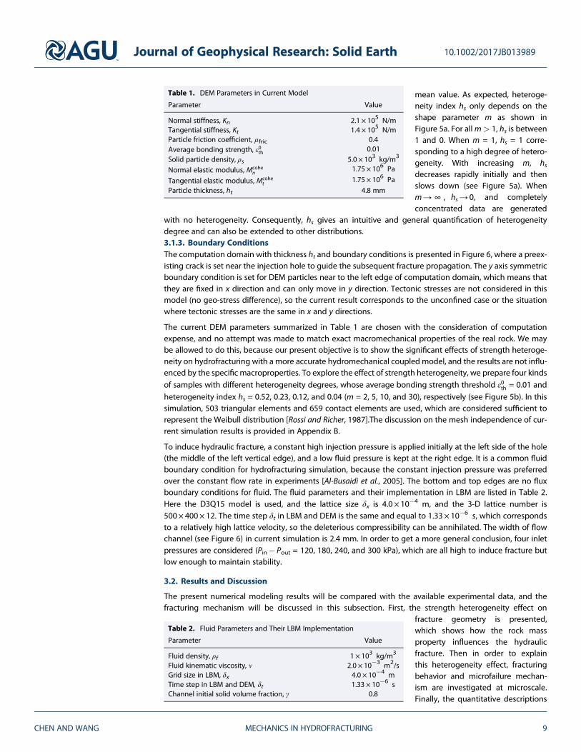
Table 1. DEM Parameters in Current Model

Parameter Value

Normal stiffness, Kn 2.1 × 105 N/mTangential stiffness, Kt 1.4 × 105 N/mParticle friction coefficient, μfric 0.4Average bonding strength, ε0th 0.01Solid particle density, ρs 5.0 × 103 kg/m3

Normal elastic modulus, Mcohen

1.75 × 106 Pa

Tangential elastic modulus, Mcohet

1.75 × 106 Pa

Particle thickness, ht 4.8 mm

Table 2. Fluid Parameters and Their LBM Implementation

Parameter Value

Fluid density, ρf 1 × 103 kg/m3

Fluid kinematic viscosity, ν 2.0 × 10�3 m2/sGrid size in LBM, δx 4.0 × 10�4 mTime step in LBM and DEM, δt 1.33 × 10�6 sChannel initial solid volume fraction, γ 0.8



of fracture geometry and failure mechanism under various pressure differences are presented, which helps toprovide a comprehensive understanding of the heterogeneity effect on hydrofracturing.3.2.1. Validation of Pressure EvolutionBefore exploring the strength heterogeneity effect, current model is further validated by recording thepressure evolution in the hole. The physical model is the same as that in Figure 6, and the fixed velocityand pressure boundary conditions are applied to the inlet and outlet of the computation domain, respec-tively. The pressure in the hole (red point in Figure 6 (1.75 cm, 8.0 cm)) is recorded during the simulation,and the evolution of dimensionless pressure increment in this point is plotted in Figure 7 (normalized bythe maximal pressure increment). It is presented that current LBM-DEM model successfully captures thepressure fluctuation during the fracture propagation (see Figure 7a), a typical pressure behavior in hydraulicfracturing tests, which is very consistent with the measured data from experiments [Cornet and Valette, 1984;Economides and Nolte, 2000]. It is because our model introduces the fracture dependent flow conductivity.When the flow conductivity becomes fracture independent, like the previous LBM-DEM models did, thepressure response with time becomes monotonically increasing, as shown in Figure 7b, which is consistentwith the previous LBM-DEM modeling results. Hence, the current model is available to be further used tostudy the heterogeneity effect on hydrofracturing.3.2.2. Strength Heterogeneity Effect on HydrofracturingIn hydrofracturing operation, fracture geometry is an essential parameter to evaluate its efficiency[Mayerhofer et al., 2010]. In the conventional reservoir, simple fracture such as single plane fracture is enough,but for an unconventional reservoir only a complex fracture network can improve its production [Mayerhoferet al., 2010]. Consequently, it is of great necessary to explore the relationship between rock mass propertiesand the hydraulic fracture geometry, so that we can predict what kind of fracture geometry tends to begenerated in a specific reservoir. Recently, some rock properties such as brittleness [Chong et al., 2010] andgeologic discontinuities [Warpinski and Teufel, 1987] have been studied, but the effect of the strength hetero-geneity, a common but essential feature in rock, on the fracture geometry has not been fully investigatedespecially quantitatively. Thus, we attempt to bridge this gap with current simulation.

The numerical modeling results of hydraulic fracture geometry in the synthetic samples with differentdegrees of heterogeneity are presented in Figures 8a–8d, which demonstrate that strength heterogeneityhas a significant effect on the complexity of hydraulic fracture. Figure 8a shows the hydraulic fracture inhighly heterogeneous sample (hs = 0.52), where many branches are generated and widely scattered in theformation, corresponding to a complex fracture geometry. However, for homogeneous sample (hs = 0.04),the fracture geometry is much simpler and few branches are observed (see Figure 8d). Figure 8b and 8c showthe fracture geometry in samples with middle degree of heterogeneity, and their fracture complexity also lieswithin the above two extremes. Because the tectonic stress is not included in current model, there is no

Figure 7. Pressure evolution curve by different methods. (a) Pressure evolution in current model where the flow conduc-tivity enhanced by new fracture is considered. It captures the pressure fluctuation owing to crack propagation, a typicalfeature in hydrofracturing test, and consistent with the measured data from experiments [Cornet and Valette, 1984;Economides and Nolte, 2000]. (b) The pressure evolution predicted when the flow conductivity becomes fractureindependent like in previous LBM-DEM scheme, which fails to capture this behavior.



predominant direction for fracture propagation just as the unconfined hydrofracturing test [Falls et al.,1992]. Another obvious difference between heterogeneous and homogeneous samples is that in highlyheterogeneous sample a lot of isolated small cracks are formed, which are not coalesced to the mainfracture (see Figure 8a). However, few isolated cracks are found in homogeneous one (see Figure 8d).Figures 8e–8h show the fluid field corresponding to the fracture geometry in Figures 8a–8d. As expected,the fracture new induced is more permeable than the surrounding rock formation, and when a connectedfracture is formed, it dominates the flow behavior.

This kind of feature has also been observed in a recent hydrofracturing experiment [Liu et al., 2016] (seeFigure 9). Figure 9a shows the hydraulic fracture in an artificial heterogeneous sample, which is more

complex than the fracture in homo-geneous one (Figure 9b). The experi-mental results in Figure 9 areobtained under the no geo-stressdifference test condition just likecurrent simulation. As a comparison,our results are also presented (seeFigures 9c and 9d). The experimentalfracture geometry of heterogeneousrock is similar to our simulationresult in heterogeneous sample withhs = 0.23, and the simple fracture inhomogeneous rock is similar to thatin current homogeneous samplewith hs = 0.04.3.2.2.1. Fracture PropagationPatternsIn order to understand this heteroge-neity controlled behavior at micro-scale, the fracturing behaviors inheterogeneous and homogeneoussamples are presented. The samplewith hs = 0.23 is taken as an exampleto show the fracture growth in het-erogeneous rock (see Figure 10).When the fluid with high pressure isinjected, the crack is first induced

Figure 9. The hydraulic fracture geometry in different rock samples, where(a) artificially heterogeneous and (b) homogeneous samples are fromReference Liu et al. [2016]. (c) The fracture geometry in current heteroge-neous sample with hs = 0.23. (d) The hydraulic fracture in homogeneoussample with hs = 0.04.

Figure 8. The fracture geometry under the pressure difference 240 kPa, with different heterogeneity index: (a) hs = 0.52,which corresponds to a highly heterogeneous sample; (b) hs = 0.23; (c) hs = 0.12; and (d) hs = 0.04, a nearly homoge-neous sample. (e–h) Color contours are the flow fields corresponding to the rock samples in Figures 8a–8d.



around the borehole (see Figure 10a). As the fracture propagates, some scattered microcracks around themain fracture is generated (see Figures 10b–10d). It is because that in heterogeneous rock, bondingstrength (εth) distribution is within a large range, and some weak bonds exist (see Figure 5b), which areeasily broken by shear force (see Figure 10j) being the small crack nucleation. Then these crack nucleationmay interact and coalesce and finally be connected to the main fracture forming new branches. As aresult, a complex hydraulic fracture is induced. Hence, the fracturing behavior in heterogeneous rock canbe summarized as the nucleation and coalescence of the small cracks. It is this particular fracturingbehavior that results in the complexity of the hydraulic fracture. However, in continuum-based model, thefracture propagation is often regarded as a continuous expansion process based on linear elastic fracturemechanics, so it is difficult to capture this discontinuous pattern of crack propagation.

Figure 10. Analysis of fracture propagation patterns in heterogeneous rock. (a–i) The fracture propagation process inheterogeneous rock with hs = 0.23 under the pressure difference of 240 kPa, which can be summarized as the formationand coalescence of crack nucleation. (j) The failure mode for each crack, where red and blue dots indicate the bondbroken by tensile failure and shear failure, respectively.

Figure 11. Analysis of fracture propagation patterns in homogeneous rock. (a–i) The fracture propagation process inhomogeneous rock with hs = 0.04 under the pressure difference of 240 kPa, where the fracture growth is achieved bycontinuous expansion of crack and corresponds to a simple fracture geometry with few branches. (j) Failure mode for eachcrack, where red and blue dots are the bonds broken by tensile failure and shear failure, respectively.



Contrary to the heterogeneous case, fracture propagation in homogeneous sample is achieved by continu-ous crack expansion with few branches (see Figure 11), which is consistent with the traditional continuumtheory. This is possibly due to the small range of bonding strength (εth) distribution in homogeneous sample,and few weak bonds exist to form crack nucleation around the main fracture. Consequently, only a simplefracture is induced in the homogeneous sample.3.2.2.2. Microfailure MechanismOver the past few decades, acoustic emissions in laboratory and field scale have been recorded to clarify themicrofailure mechanism of hydraulic fracture [Falls et al., 1992; Stoeckhert et al., 2015; Talebi and Cornet, 1987],and one of the major findings is that shear failure seismicity is commonly recorded and even in some cases itdominates the failure behavior [Al-Busaidi et al., 2005]. However, this observation is not consistent with tensilefracture suggested by traditional analytical and numerical models, and the conflict has not been fully solved[Al-Busaidi et al., 2005; Ishida et al., 1997; Shimizu et al., 2011]. In current simulation, shear failure eventsare also observed (see Figures 10j and 11j) just as experimental observations. Figure 12 shows the variationof shear and tensile failure events during hydrofracturing. It is presented that strength heterogeneityalso has an influence on microfailure mechanism. Shear failure dominates the fracturing behavior in theheterogeneous sample (see Figure 12a), but in the homogeneous sample tensile failure events more easilyoccur (see Figure 12b). Similar scenarios can also be found in a recent hydrofracturing experiment[Stoeckhert et al., 2015].

For a deep understanding of this phenomenon, fracture propagation pattern and microfailure mechanismare analyzed simultaneously. It is presented that shear failure is usually accompanied by forming crack

nucleation and connecting it tothe main fracture, which moreeasily happens in heterogeneousrock (see Figure 10j). Similar resultsabout the role of shear failure inhydrofracturing were also obtainedby laboratory and field experi-ments [Ishida, 2001; Talebi andCornet, 1987]. In contrary, tensilefailure events are often accompa-nied by continuous expansion ofthe crack (see Figure 11j), which iscommonly observed in homoge-neous rock. The above discussionmay help us understand the con-flict between experimental obser-vations and continuum theory

Figure 12. Variation of shear and tensile failure events in (a) heterogeneous sample (hs = 0.23) and (b) homogeneous sam-ple (hs = 0.04) under the pressure difference of 240 kPa.

Figure 13. Two extreme structures for root system. (a) Herringbone branch-ing corresponds to a low degree of branching growth and can be regardedas a simple fracture geometry. (b) Dichotomous branching is a highdegree of branching growth with high geometric complexity.



predictions. In continuum model, it isusually assumed that the fracturepropagation is achieved by continu-ous expansion of the crack, andunder this condition tensile fractur-ing is indeed the main failuremechanism just as presented in thehomogeneous sample (Figure 11j).However, this assumption may beno longer valid in real rock with highheterogeneity degree, where thefracture propagation is not continu-ous and often accompanied by shearfailure. Thus, the traditional modelcannot effectively predict the fractur-ing behavior and failure mechanismin real rock.3.2.3. Quantitative Description ofFracture Geometry andFailure MechanismThe above discussions are mainlyqualitative and under the pressure

difference of 240 kPa. In this subsection, quantitative descriptions of fracture geometry and failure mechan-ism with various pressure differences (120 kPa, 180 kPa, 240 kPa and 300 kPa) are considered, which helps toprovide a comprehensive understanding of the heterogeneity effect on hydrofracturing.

Quantitative analysis of fracture geometry is an important aspect of studying the cracking behavior of rock[Liu et al., 2013] and evaluating the hydrofracturing operation [Mayerhofer et al., 2010]. However, owing tothe complexity of fracture geometry, current analysis is still limited to the quantification of basic geometricparameters of the fracture such as fracture length, fracture density, and fractal dimension [Liu et al., 2013],and none of them can reflect the morphology of fracture geometry directly and effectively. Thus, how todefine an index to quantify the fracture geometry is of great significance but also difficult.

In current simulation, the hydraulic fracture is mainly a “tree”-type fracture. Consequently, the topologicalindex (q) for tree-type structure is introduced to quantify the hydraulic fracture in current simulation, whichwas originally used to describe the geometry of root system [Bouma et al., 2001; Oppelt et al., 2001]. In rootsystem, there are two extreme structures, herringbone branching (Figure 13a) and dichotomous branching(Figure 13b). Herringbone branching is a simple structure with low degree of the branching growth anddevelopment. On the contrary, dichotomous branching corresponds to a high degree of the branchinggrowth and can be regarded as an ideal hydraulic fracture with high geometric complexity. The topologicalindex (q) is such a parameter to quantify branching patterns between the above two extremes [Oppelt et al.,2001]. When q = 0, the fracture corresponds to the dichotomous branching. With increasing q, it graduallytransforms to the herringbone branching. When q = 1, an exact herringbone branching is formed.However, the original topological index (q) defined inOppelt et al. [2001] may be smaller than 0 in some cases,so a modified topological index (qm) is proposed to make it between 0 and 1 strictly and written as

qm ¼ bm � bminm

bmaxm � bmin

m

; bminm ¼ ln ν0 þ 0:5ν1ð Þ

ln2� 1; bmax

m ¼ ν0 þ 12

þ 1� 1ν0

þ ν1 þ ν1 þ 1ð Þν12ν0

; (20)

where ν0 is the number of external vertices (with outdegree 0), ν1 the number of vertices with outdegree 1,and bm the average topological depth. Confined to the length of the article, more details about modifiedtopological index (qm) are provided in Appendix A.

Figure 14 shows the modified topological index of the hydraulic fracture in homogeneous (hs = 0.04) and het-erogeneous (hs = 0.23) samples with various pressure differences. Under the same pressure difference, qm in

Figure 14. Modified topological index (qm) for homogeneous (red one withhs = 0.04) and heterogeneous (blue one with hs = 0.23) samples undervarious pressure differences (120 kPa, 180 kPa, 240 kPa, 300 kPa), and inorder to avoid the random error, five random samples are generated for eachstrength heterogeneity degree.



the heterogeneous sample is alwayssmaller than that in the homoge-neous one, which demonstrateshigher degree of branching growthand development is achieved in het-erogeneous samples just as dis-cussed in section 3.2.2. On the otherhand, it also shows the feasibilityand effectiveness of modified topolo-gical index (qm) in quantitativedescription of fracture complexity. Inaddition, it is qm that makes it possi-ble to study pressure differenceeffects on hydraulic fracture in sam-ples with different heterogeneitydegrees. For heterogeneous samples(hs = 0.23), with increasing pressuredifference, the complexity of the frac-ture increases initially and thenremains constant (blue dash line inFigure 14). However, for homoge-neous samples (hs = 0.04), the frac-

ture complexity does not increase until a relatively high pressure difference reaches (red dash line inFigure 14). In heterogeneous samples, some bonds with weak bonding strength exist, which make failureevents sensitive to the pressure difference, and the fracture complexity increases immediately with theincreasing pressure difference. However, few weak bonds exist in the homogeneous sample, so only a rela-tively high pressure difference can break the bonds around the fracture tip (being crack nucleation), which isnecessary to form a complex fracture. In current simulation, this critical value is 240 kPa, and only pressuredifference larger than it can lead to a more complex fracture.

Similar analysis is also applied to the heterogeneity effect on microfailure mechanism. Shear failure percen-tages in homogeneous and heterogeneous samples with various pressure differences are shown inFigure 15. It is presented that the microfailure mechanism is affected by two factors. The first one is thestrength heterogeneity degree of the sample. Under the same pressure difference, shear failure more easilydominates in heterogeneous samples than in homogeneous ones as presented in section 3.2.2.2. Another

important factor is the pressuredifference, which reflects the influ-ence of fluid phase on microfailuremechanism. For both heterogeneousand homogeneous samples, shearfailure percent increases withincreasing pressure difference, whichmeans high-pressure difference isconducive to shear failure events.This may be due to the high porepressure in the matrix around thefracture caused by the fluid leakoffunder high-pressure difference.

This pore pressure effect on failuremechanism can be further explainedgraphically by the Mohr-Coulombfailure criterion as shown inFigure 16. For a certain point withgreatest principal stress σ1 and least

Figure 15. Shear failure fraction in heterogeneous (hs = 0.23) and homoge-neous (hs = 0.04) samples under various pressure differences, and for eachheterogeneity degree, five random samples with the same distributionare generated.

Figure 16. Mohr-Coulomb failure criterion diagram in the saturatedmaterial,when Mohr’s circle becomes tangent to the failure envelop, shear failure willresult. If the pore pressure increases, Mohr’s circle moves to the left, soshear failure events more easily occur.



principal stress σ3, its normal and shear force in different directions can be represented graphically by Mohr’scircle with center (σ1 + σ3)/2 and radius (σ1� σ3)/2. If the Mohr’s circle becomes tangent to the failure envelop(straight line in Figure 16), shear failure will result. In a saturated material, stress should be replaced by theeffective stress σeff (σeff = σ� p), so the center and radius of Mohr’s circle become (σ1 + σ3� 2p)/2 and(σ1� σ3)/2, respectively. When the pore pressure increase (Δp), the Mohr’s circle will move to the left byΔp (see Figure 16). As a result, Mohr’s circle becomes more likely to be tangent to the failure envelop, leadingto a shear failure event. Chitrala et al. [2012a, 2012b] studied the effect of flow rate and fluid viscosity onfailure mechanism [Chitrala et al., 2012a, 2012b], and both of them can be summarized as higher pore pres-sure more easily leads to shear failure.

4. Conclusions

In this study, a pore-scale LBM-DEM framework is presented to simulate hydrofracturing directly and aimedto provide a more accurate hydromechanical coupled model to capture the multiphysics and complex geol-ogy in this process. As a first step, the strength heterogeneity effect on fracture geometry and microfailuremechanism is simulated. Contrary to the traditional continuummodel, the cracks nucleation and coalescencecan be simulated explicitly. In order to evaluate the hydraulic fracture quantitatively, a modified topologicalindex is proposed to quantify the complexity of fracture geometry, which can directly reflect the morphologyof fracture geometry effectively unlike other basic geometric parameters such as fracture length, fracturedensity, and fractal dimension. Numerical results show that strength heterogeneity has a significant influenceon hydrofracture process. In heterogeneous sample fracture geometry is more complex than that inhomogeneous one. In addition, shear failure is more easily observed in heterogeneous sample with highpore pressure.

Current numerical results may provide some basic understanding of hydrofracturing process at pore scale,including failure mechanism and fracture geometry.

1. There are two kinds of fracturing behavior in rock during hydrofracturing. The first one is crack nucleationaround the fracture tip and then connection of it to the main fracture, which is commonly observed inheterogeneous sample and accompanied by shear failure. The second one is the continuous propagationof the crack in homogeneous sample, where tensile failure usually dominates. In addition, these two fail-ure patterns in hydrofracturing are also affected by the pore pressure. As the pore pressure increases, thefracturing behavior tends to transform from the second one to the first one. Thus, traditional continuummodels with continuous crack propagation assumption difficultly predict the complex fracturing behavior(crack nucleation and coalescence) in real rock, which results in the conflict between its prediction (tensilefailure) and experimental observation (shear failure).

2. The strength heterogeneity in rock mass has a significant effect on the complexity of hydraulic fracture. Ina highly heterogeneous rock, weak bonds (preexisting defects in rock) around the fracture tip are easilybroken by shear force. Once they are connected to the main fracture, new branches are formed, resultingin complex fracture geometry. Thus, before hydraulic fracture treatment, the degree of strength hetero-geneity in the formation can be used to predict whether a complex fracture can be induced or not, whichmay serve as the first step to evaluate a reservoir especially for unconventional ones, because only a com-plex fracture can stimulate their productions efficiently.

Appendix A: Modified Topological Index

The calculation of the modified topological index is provided in this section. For a branching structure, thereare two kinds of elements, vertices and edges, and each edge connects two vertices. Here the branchingstructure is also called as a tree-type structure. The fracture geometry in our simulations is close to thetree-type structure; thus, the quantitative description of the “tree” structure can be introduced to quantifyour fracture geometry.

A tree structure is given graphically as an example in Figure A1, where vertices i is the base vertex and theedge not emerging from the base vertex has indegree 1 (mother edge) and can have various outdegrees(the number of adjacent daughter edges) [Oppelt et al., 2001].



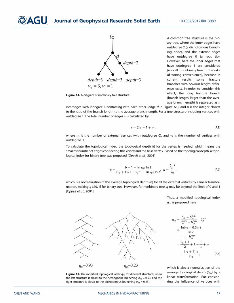
A common tree structure is the bin-ary tree, where the inner edges haveoutdegree 2 (a dichotomous branch-ing node), and the exterior edgeshave outdegree 0 (a root tip).However, here the inner edges thathave outdegree 1 are considered(we call it nonbinary tree for the sakeof writing convenience), because incurrent results some fracturebranches with obvious length differ-ence exist. In order to consider thiseffect, the long fracture branch(branch length larger than the aver-age branch length) is separated as n

interedges with indegree 1 contacting with each other (edge d in Figure A1), and n is the integer closestto the ratio of the branch length to the average branch length. For a tree structure including vertices withoutdegree 1, the total number of edges ν is calculated by

ν ¼ 2ν0 � 1þ ν1; (A1)

where ν0 is the number of external vertices (with outdegree 0), and ν1 is the number of vertices withoutdegree 1.

To calculate the topological index, the topological depth (l) for the vertex is needed, which means thesmallest number of edges connecting this vertex and the base vertex. Based on the topological depth, a topo-logical index for binary tree was proposed [Oppelt et al., 2001]

q ¼ b� 1� ln ν0= ln 2ν0 þ 1ð Þ=2� ν0�1 � ln ν0= ln 2

; b ¼Pν0

l

ν0; (A2)

which is a normalization of the average topological depth (b) for all the external vertices by a linear transfor-mation, making q ∈ [0, 1] for binary tree. However, for nonbinary tree, q may be beyond the limit of 0 and 1[Oppelt et al., 2001].

Thus, a modified topological indexqm is proposed here

qm ¼ bm � bminm

bmaxm � bmin

m

; bminm

¼ ln ν0 þ 0:5ν1ð Þln 2

� 1; bmaxm

¼ ν0 þ 12

þ 1� 1ν0

þ ν1

þ ν1 þ 1ð Þν12ν0

; (A3)

which is also a normalization of theaverage topological depth (bm) by alinear transformation. For conside-ring the influence of vertices with

Figure A2. The modified topological index qm for different structure, wherethe left structure is closer to the herringbone branching qm = 0.93, and theright structure is closer to the dichotomous branching qm = 0.23.

Figure A1. A diagram of nonbinary tree structure.



outdegree 1, the average topologicaldepth bm is modified as

bm ¼Pν0

l þPν1l

ν0; (A4)

where the topological depth issummed for both vertices with out-degree 0 and ones with outdegree 1.

With this modification, qm ∈ [0, 1] forboth binary tree and nonbinary tree,and qm can recover q for binary tree.When qm→ 0, the tree structure iscloser to the dichotomous branching(see Figure 13b), and when qm→ 1, it

is closer to herringbone branching (see Figure 13a). Figure A2 shows two structures and their modified topo-logical index qm, which presents that the current modified topological index can effectively distinguish theherringbone branching from herringbone branching.

Appendix B: Mesh Independence Discussion

To show the mesh independence of current numerical results, the same case as that in Figure 6 is simu-lated with finer meshes (989 elements, see Figure B1). Here we consider two samples (hs = 0.23 and 0.04)with fluid pressure difference of 240 kPa. Owing to the random factor introduced by Weibull distributionof bonding strength, the fracture geometry may be not completely identical under different meshmorphologies. However, the underlying physics of strength heterogeneity effects on hydrofracturingare not influenced by the specific mesh size. As present in Figure B2, fracture geometry is much morecomplex in the heterogeneous sample (hs = 0.23) than that in the homogeneous one (hs = 0.04), whichis the same as the results obtained in section 3.2.2. In addition, the model with finer meshes alsoconfirms the conclusion that shear failure more easily dominates in heterogeneous samples (hs = 0.23,shear failure percent 53.33%) than in homogeneous ones (hs = 0.04, shear failure percent 25%). Thus,the numerical results obtained from coarse mesh model (503 elements) are robust and can be used forfurther exploration.

Figure B1. The diagram of LBM-DEM model with finer meshes, where 989elements and 1309 contact elements are generated.

Figure B2. The fracture geometry obtained by current LBM-DEM model with finer meshes, and the pressure difference is240 kPa. (a) Hydraulic fracture in the homogeneous sample (hs = 0.04) and (b) in the heterogeneous sample (hs = 0.23).



ReferencesAdachi, A., E. Siebrits, A. Peirce, and J. Desroches (2007), Computer simulation of hydraulic fractures, Int. J. Rock Mech. Min. Sci., 44(5), 739–757.Al-Busaidi, A., J. F. Hazzard, and R. P. Young (2005), Distinct element modeling of hydraulically fractured Lac du Bonnet granite, J. Geophys.

Res., 110, B06302, doi:10.1029/2004JB003297.Barbati, A. C., J. Desroches, A. Robisson, and G. H. McKinley (2016), Complex fluids and hydraulic fracturing, Annu. Rev. Chem. Biomol. Eng., 7,

415–453.Bouma, T., K. L. Nielsen, J. Van Hal, and B. Koutstaal (2001), Root system topology and diameter distribution of species from habitats differing

in inundation frequency, Funct. Ecol., 15(3), 360–369.Boutt, D., B. Cook, and J. Williams (2011), A coupled fluid–solid model for problems in geomechanics: Application to sand production, Int. J.

Numer. Anal. Methods Geomech., 35(9), 997–1018.Bruno, M., A. Dorfmann, K. Lao, and C. Honeger (2001), Coupled particle and fluid flow modeling of fracture and slurry injection in weakly

consolidated granular media, paper presented at DC Rocks 2001, The 38th US Symposium on Rock Mechanics (USRMS), American RockMechanics Association.

Chen, S., and G. D. Doolen (1998), Lattice Boltzmann method for fluid flows, Annu. Rev. Fluid Mech., 30(1), 329–364.Chen, Y., Q. Cai, Z. Xia, M. Wang, and S. Chen (2013), Momentum-exchange method in lattice Boltzmann simulations of particle-fluid

interactions, Phys. Rev. E, 88(1), 013303.Chen, Y., Q. Kang, Q. Cai, M. Wang, and D. Zhang (2015), Lattice Boltzmann simulation of particle motion in binary immiscible fluids,

Commun. Comput. Phys., 18(03), 757–786.Chen, Z., C. Xie, Y. Chen, and M. Wang (2016), Bonding strength effects in hydro-mechanical coupling transport in granular porous media by

pore-scale modeling, Computation, 4(1), 15, doi:10.3390/computation4010015.Chitrala, Y., C. Sondergeld, and C. Rai (2012a), Acoustic emission studies of hydraulic fracture evolution using different fluid viscosities, paper

presented at 46th US Rock Mechanics/Geomechanics Symposium, American Rock Mechanics Association.Chitrala, Y., C. H. Sondergeld, and C. S. Rai (2012b), Microseismic studies of hydraulic fracture evolution at different pumping rates, paper

presented at SPE Americas Unconventional Resources Conference, Society of Petroleum Engineers.Chong, K. K., O. A. Jaripatke, W. V. Grieser, and A. Passman (2010), A completions roadmap to shale-play development: A review of successful

approaches toward shale-play stimulation in the last two decades, paper presented at International Oil and Gas Conference andExhibition in China, Society of Petroleum Engineers.

Cornet, F., and B. Valette (1984), In situ stress determination from hydraulic injection test data, J. Geophys. Res., 89(B13), 11,527–11,537,doi:10.1029/JB089iB13p11527.

Cundall, P. A., and O. D. Strack (1979), A discrete numerical model for granular assemblies, Geotechnique, 29(1), 47–65.Detournay, E. (2016), Mechanics of hydraulic fractures, Annu. Rev. Fluid Mech., 48, 311–339.Economides, M. J., and K. G. Nolte (2000), Reservoir Stimulation, chap. 1, pp. 1–30, Wiley, Chichester, U. K.Eshiet, K. I., Y. Sheng, and J. Ye (2013), Microscopic modelling of the hydraulic fracturing process, Environ. Earth Sci., 68(4), 1169–1186.Falls, S., R. Young, S. Carlson, and T. Chow (1992), Ultrasonic tomography and acoustic emission in hydraulically fractured Lac du Bonnet grey

granite, J. Geophys. Res., 97(B5), 6867–6884, doi:10.1029/92JB00041.Fortes, A. F., D. D. Joseph, and T. S. Lundgren (1987), Nonlinear mechanics of fluidization of beds of spherical particles, J. Fluid Mech., 177,

467–483.Furtney, J., F. Zhang, and Y. Han (2013), Review of methods and applications for incorporating fluid flow in the discrete element method,

paper presented at Proceedings of the 3rd International FLAC/DEM Symposium, Hangzhou, China.Galindo-Torres, S., D. Pedroso, D. Williams, and L. Li (2012), Breaking processes in three-dimensional bonded granular materials with general

shapes, Comput. Phys. Commun., 183(2), 266–277.Geertsma, J., and F. De Klerk (1969), A rapid method of predicting width and extent of hydraulically induced fractures, J. Pet. Technol., 21(12),

1571–1581.Glowinski, R., T. Pan, T. Hesla, D. Joseph, and J. Periaux (2001), A fictitious domain approach to the direct numerical simulation of

incompressible viscous flow past moving rigid bodies: Application to particulate flow, J. Comput. Phys., 169(2), 363–426.Gou, Y., L. Zhou, X. Zhao, Z. Hou, and P. Were (2015), Numerical study on hydraulic fracturing in different types of georeservoirs with

consideration of H2M-coupled leak-off effects, Environ. Earth Sci., 73(10), 6019–6034.Hazzard, J. F., R. P. Young, and S. J. Oates (2002), Numerical modeling of seismicity induced by fluid injection in a fractured reservoir, paper

presented at Mining and Tunnel Innovation and Opportunity, Proceedings of the 5th North American Rock Mechanics Symposium,Toronto, Canada, Citeseer.

Ishida, T. (2001), Acoustic emission monitoring of hydraulic fracturing in laboratory and field, Constr. Build. Mater., 15(5), 283–295.Ishida, T., Q. Chen, and Y. Mizuta (1997), Effect of injected water on hydraulic fracturing deduced from acoustic emission monitoring,

Pure Appl. Geophys., 150, 627–646.Ishida, T., Q. Chen, Y. Mizuta, and J. C. Roegiers (2004), Influence of fluid viscosity on the hydraulic fracturing mechanism, J. Energy Resour.

Technol., 126(3), 190–200.Kovalyshen, Y. (2010), Fluid-driven fracture in poroelastic medium, Ph.D thesis, Univ. of Minnesota.Latham, J. P., J. Xiang, M. Belayneh, H. M. Nick, C. F. Tsang, and M. J. Blunt (2013), Modelling stress-dependent permeability in fractured rock

including effects of propagating and bending fractures, Int. J. Rock Mech. Min. Sci., 57, 100–112.Lisjak, A., O. Mahabadi, B. Tatone, K. Alruwaili, G. Couples, J. Ma, and A. Al-Nakhli (2015), 3D simulation of fluid-pressure-induced fracture

nucleation and growth in rock samples, paper presented at 49th US Rock Mechanics/Geomechanics Symposium, American RockMechanics Association.

Liu, C., C. S. Tang, B. Shi, and W. B. Suo (2013), Automatic quantification of crack patterns by image processing, Comput. Geosci., 57,77–80.

Liu, P., Y. Ju, P. G. Ranjith, Z. Zheng, and J. Chen (2016), Experimental investigation of the effects of heterogeneity and geostress difference onthe 3D growth and distribution of hydrofracturing cracks in unconventional reservoir rocks, J. Nat. Gas Sci. Eng., 35, 541–554.

Ma, G., Q. Wang, X. Yi, and X. Wang (2014), A modified SPH method for dynamic failure simulation of heterogeneous material, Math. Probl.Eng., 2014, 808359.

Ma, G., X. Wang, and F. Ren (2011), Numerical simulation of compressive failure of heterogeneous rock-like materials using SPH method,Int. J. Rock Mech. Min. Sci., 48(3), 353–363.

Mahabadi, O., B. Tatone, and G. Grasselli (2014), Influence of microscale heterogeneity and microstructure on the tensile behavior ofcrystalline rocks, J. Geophys. Res. Solid Earth, 119, 5324–5341, doi:10.1002/2014JB011064.



AcknowledgmentsThe data for this paper are availablefrom M. Wang for free. This work isfinancially supported by the NSF grantof China (U1562217), National Scienceand Technology Major Project on Oiland Gas (2017ZX05013001), thePetroChina Innovation Foundation(2015D-5006-0201), and the TsinghuaUniversity Initiative Scientific ResearchProgram (2014z22074). The authorswant to acknowledge the open sourcelibrary MechSys developed by S.A.Galindo Torres (http://mechsys.nongnu.org/index.shtml).

https://doi.org/10.1029/2004JB003297

https://doi.org/10.3390/computation4010015

https://doi.org/10.1029/JB089iB13p11527

https://doi.org/10.1029/92JB00041

https://doi.org/10.1002/2014JB011064

http://mechsys.nongnu.org/index.shtml

http://mechsys.nongnu.org/index.shtml

Mayerhofer, M. J., E. Lolon, N. R. Warpinski, C. L. Cipolla, D. W. Walser, and C. M. Rightmire (2010), What is stimulated reservoir volume?,SPE Prod. Oper., 25(01), 89–98.

McClintock, F., and F. Zaverl Jr. (1979), An analysis of the mechanics and statistics of brittle crack initiation, Int. J. Fract., 15(2), 107–118.Ni, X. D., C. Zhu, and Y. Wang (2015), Hydro-mechanical analysis of hydraulic fracturing Based on an improved DEM-CFD coupling model at

micro-level, J. Comput. Theor. Nanosci., 12(9), 2691–2700.Nick, H., A. Paluszny, M. Blunt, and S. Matthai (2011), Role of geomechanically grown fractures on dispersive transport in heterogeneous

geological formations, Phys. Rev. E, 84(5), 056301.Noble, D., and J. Torczynski (1998), A lattice-Boltzmann method for partially saturated computational cells, Int. J. Modern Phys. C, 9(08),

1189–1201.Nordgren, R. (1972), Propagation of a vertical hydraulic fracture, Soc. Pet. Eng. J., 12(04), 306–314.Oppelt, A. L., W. Kurth, and D. L. Godbold (2001), Topology, scaling relations and Leonardo’s rule in root systems from African tree species,

Tree Physiol., 21(2), 117–128.Qian, Y. H., D. Dhumieres, and P. Lallemand (1992), Lattice BGK model for Navier-Stokes equation, Europhys. Lett., 17(6), 479–484.Qiu, K., N. Cheng, X. Ke, Y. Liu, L. Wang, Y. Chen, Y. Wang, and P. Xiong (2013), 3D reservoir geomechanics workflow and its application to a

tight gas reservoir in western China, paper presented at IPTC 2013: International Petroleum Technology Conference.Rahman, M., and M. Rahman (2010), A review of hydraulic fracture models and development of an improved pseudo-3D model for

stimulating tight oil/gas sand, Energy Sour. Part A: Recovery, Util. Environ. Effects, 32(15), 1416–1436.Rossi, P., and S. Richer (1987), Numerical modelling of concrete cracking based on a stochastic approach, Mater. Struct., 20(5), 334–337.Sharma, N., and N. A. Patankar (2005), A fast computation technique for the direct numerical simulation of rigid particulate flows, J. Comput.

Phys., 205(2), 439–457.Sheng, Y., M. Sousani, D. Ingham, and M. Pourkashanian (2015), Recent developments in multiscale and multiphase modelling of the

hydraulic fracturing process, Math. Probl. Eng., 2015, 729672.Shimizu, H., S. Murata, and T. Ishida (2011), The distinct element analysis for hydraulic fracturing in hard rock considering fluid viscosity and

particle size distribution, Int. J. Rock Mech. Min. Sci., 48(5), 712–727.Stoeckhert, F., M. Molenda, S. Brenne, and M. Alber (2015), Fracture propagation in sandstone and slate—Laboratory experiments, acoustic

emissions and fracture mechanics, J. Rock Mech. Geotech. Eng., 7(3), 237–249.Strack, O. E., and B. K. Cook (2007), Three-dimensional immersed boundary conditions for moving solids in the lattice-Boltzmann method,

Int. J. Numer. Methods Fluids, 55(2), 103–125.Succi, S. (2001), The Lattice Boltzmann Equation: For Fluid Dynamics and Beyond, chap. 1, pp. 3–15, Oxford Univ. Press, Oxford, U. K.Talebi, S., and F. H. Cornet (1987), Analysis of the microseismicity induced by a fluid injection in a granitic rock mass, Geophys. Res. Lett., 14(3),

227–230, doi:10.1029/GL014i003p00227.Tang, C., H. Liu, P. Lee, Y. Tsui, and L. Tham (2000), Numerical studies of the influence of microstructure on rock failure in uniaxial compression

—Part I: Effect of heterogeneity, Int. J. Rock Mech. Min. Sci., 37(4), 555–569.Thallak, S., L. Rothenburg, and M. Dusseault (1991), Simulation of multiple hydraulic fractures in a discrete element system, paper presented

at The 32nd US Symposium on Rock Mechanics (USRMS), American Rock Mechanics Association.Veatch, R., Jr., and Z. Moschovidis (1986), An overview of recent advances in hydraulic fracturing technology, paper presented at

International Meeting on Petroleum Engineering, Society of Petroleum Engineers.Wang, M., and S. Chen (2007), Electroosmosis in homogeneously chargedmicro-and nanoscale random porousmedia, J. Colloid Interface Sci.,

314(1), 264–273.Wang, M., J. Wang, N. Pan, and S. Chen (2007), Mesoscopic predictions of the effective thermal conductivity for microscale random porous

media, Phys. Rev. E, 75(3), 036702.Wang, T., W. Zhou, J. Chen, X. Xia, Y. Li, and X. Zhao (2014), Simulation of hydraulic fracturing using particle flowmethod and application in a

coal mine, Int. J. Coal Geol., 121, 1–13.Wang, Z., X. Jin, X. Wang, L. Sun, and M. Wang (2016), Pore-scale geometry effects on gas permeability in shale, J. Nat. Gas Sci. Eng., 34,

948–957.Warpinski, N., and L. Teufel (1987), Influence of geologic discontinuities on hydraulic fracture propagation, J. Pet. Technol., 39(02), 209–220.Yardley, B. W. (1983), Quartz veins and devolatilization during metamorphism, J. Geol. Soc., 140(4), 657–663.Yew, C. H., and X. Weng (2014), Mechanics of Hydraulic Fracturing, chap. 2, pp. 23–47, Gulf Professional Publishing, Oxford, U. K.Zhang, L., and M. Wang (2015), Modeling of electrokinetic reactive transport in micropore using a coupled lattice Boltzmann method,

J. Geophys. Res. Solid Earth, 120, 2877–2890, doi:10.1002/2014JB011812.Zhang, X., D. J. Sanderson, and A. J. Barker (2002), Numerical study of fluid flow of deforming fractured rocks using dual permeability model,

Geophys. J. Int., 151(2), 452–468.Zhou, L., and M. Z. Hou (2013), A new numerical 3D-model for simulation of hydraulic fracturing in consideration of hydro-mechanical

coupling effects, Int. J. Rock Mech. Min. Sci., 60, 370–380.Zhou, L., M. Z. Hou, Y. Gou, andM. Li (2014), Numerical investigation of a low-efficient hydraulic fracturing operation in a tight gas reservoir in

the North German Basin, J. Pet. Sci. Eng., 120, 119–129.Zhu, W., and O. Bruhns (2008), Simulating excavation damaged zone around a circular opening under hydromechanical conditions, Int. J.

Rock Mech. Min. Sci., 45(5), 815–830.



https://doi.org/10.1029/GL014i003p00227

https://doi.org/10.1002/2014JB011812

pore-scale modeling of hydromechanical coupled mechanics ... fracturing.pdf · pore-scale modeling...

Documents