precise modelling of a gantry crane system including · pdf fileissn : 2319 – 3182,...

ISSN : 2319 – 3182, Volume-2, Issue-1, 2013

119

Precise Modelling of a Gantry Crane System Including Friction, 3D

Angular Swing and Hoisting Cable Flexibility

Renuka V. S.

& Abraham T Mathew

Electrical Engineering Department, NIT Calicut E-mail : [email protected] , [email protected]

Abstract - A crane system offers a typical control problem

being an under actuated MIMO system. In this paper the

precise modelling of a 2D gantry crane system with 3 DOF

is considered. First a simple dynamic model of the system

is obtained using Lagrange’s equations of motion. Then,

friction non-linearities were added to the model, which

were found to decrease the output magnitudes from

reference values. The model was further improved by

considering the possibility of 3D angular swing which

showed more accurate transient responses. Finally, the

dynamics of hoisting cable flexibility was added to the

system resulting in a complex model requiring time

consuming simulation. But, significant change was seen in

the angular swing output which will significantly affect

controller performance. The models considering either

flexibility or 3D load swing are comparatively less complex

than the combined model. The precise model to be

considered is a trade-off between safety (minimum swing

angle) and precise load handling.

Keywords— Gantry crane system, degree of freedom, Euler-

Bernoulli beam equation, Lagrangian equation, friction

model, cable flexibility

I. INTRODUCTION

For modelling purposes, the gantry crane system is

considered as a trolley-pendulum system. Two types of

crane modelling can be identified viz. Distributed mass

and lumped mass models [1]. Distributed mass model is

valid only when payload mass is of the same order of

magnitude as the cable and trolley displacement and

cable angle are small.

Lumped mass modelling is the most widely used

approach in which the hoisting line is modelled as a

mass less cable. The payload is lumped with the hook

and modelled as a point mass. The cable-hook-payload

assembly is modelled as a spherical pendulum. The

resulting mathematical representation is simple and

compact while capturing the complex dynamics of the

payload motion. Lumped mass models are of two types

„reduced models‟ (all external excitations are lumped

into the motion of the suspension point) and extended

models (crane support mechanism and platform are

added to the dynamic crane model) [1]. Gantry cranes

are usually used in fixed sites inside a factory and

therefore a reduced model is the most suitable.

A 2D trolley crane system transport loads in 2D, i.e.

it can lift the load and move it in one horizontal

direction. The torques required to move the trolley and

to lift the load are generated using two motors, namely

trolley and hoist motors. The friction occurring in the

linear actuator and in the trolley motor has a very

significant effect on the system behaviour. Empirical

approach can be taken to model friction in a system by

reproducing effects observed in experiments. There are

different interpretations of friction and accordingly

different models are available in literature.The LuGre

friction model can capture most of the friction behaviour

that has been, in general, observed experimentally in

control systems [2].

To include the effect of flexibility of the hoisting

cable additional displacement of the load due to the

flexibility of the cable need to be found out. Solution of

Euler-Bernoulli beam equation for a loaded beam, using

assumed mode method [3] is one method to find

deflection due to flexibility.

Payloads are very heavy and payload pendulations

concerns the safety in the workspace and structural

integrity of the crane. Thus payload pendulations need

to be suppressed throughout the travel path which is a

major challenge as no direct control is possible. These

unwanted motions can arise as a result of inertia forces

(due to motion of payload), base excitations (due to

motion of the supporting structure) and/or disturbances

on payload (such as wind) [1]. Closed loop techniques

International Journal on Theoretical and Applied Research in Mechanical Engineering (IJTARME)


120

are particularly designed to counter the inertia

excitations. The control input here is the force or torque

applied to the trolley and girder motor (where available)

in order to suppress pendulations due to acceleration and

deceleration of the trolley. Linear feedback controllers

are closed loop control techniques tuned to counter the

effects of the natural frequency of the cable-payload

assembly, and are thus sensitive to cable length

variations. Even though dealing with a linear model is

far less complex, neglecting the non linearities may

significantly impact the performance of a linear

controller. Thus, non-linear controllers are found to be

more robust.

For the successful sway suppression and hoist

control of a suspended load, it is important to know

what part of the crane dynamics should be included in

the control law design process and what part can be

neglected [4].

II. DYNAMIC MODELLING OF A GANTRY

CRANE SYSTEM

A 3 degree of freedom 2D gantry crane is modelled

here. The system is a two input three output system.

A. 2d Non-Linear Model With Load Hoisting

Fig 1 shows the swing motion of the load caused by

trolley movement of a 3 degree of freedom

(displacement of trolley, angular swing of payload and

hoist cable length) gantry crane system. The trolley and

the load are considered as point masses and are assumed

to move in a 2D plane. Here, X is trolley moving

direction Z is vertical direction, θ (t) is the sway angle

of the load (rad), x(t) is displacement of the trolley (m),

l(t) is hoist cable length in meters, Fx is control force

applied to the trolley in the X-direction (N), Fl is control

force applied to the payload in the l direction (N), mp is

payload mass(kg), and I is mass moment of inertia of the

payload (kgm2).

Fig 1. Trolley-Cart 2D model of gantry crane system with

load hoisting[4]

For the under actuated system, forces Fx and Fl are

the two inputs and trolley displacement x, angular swing

θ and hoist cable length are the three outputs.

The following assumptions are made for deriving

the dynamic equations of the model: i) the payload and

trolley are connected by a mass less rigid cable. ii) the

trolley and payload mass and the position of the trolley

are known. iii) all frictional elements in the trolley and

hoist motions can be neglected. iv) the rod elongation is

negligible. v) trolley and load moves in a 2D plane. vii)

viscous damping is neglected. vii) external disturbances

such as wind are neglected. The coordinates of the

payload is (xp, zp ) and is given by,

xp = x + lsinθ , zp = −lcosθ (1)

The kinetic and potential energies of the system are

given by

where

(3)

Substituting,

(4)

For the given system, the generalised coordinate vector

q and force vector F are given by,

q(t) = [x(t) l(t) θ(t)]T

(5)

Using the above equations Lagrange equations for the

system is obtained as,

(2)



121

B. Friction Model

To derive appropriate friction model from physical

laws alone is impossible. Empirical approach can be

taken to model friction in a system by reproducing

effects observed in experiments. Among different

interpretations of friction the Lu-Gre friction model is

found to capture most of the friction behaviour that has

been, in general, observed experimentally in control

systems [2].

The friction occurring in the linear actuator and in

the trolley motor has a very significant effect on the

system behaviour. The hoist motor friction is mainly due

to the gear. The efficiency of the hoist motor with the

attached gear box is 50 % for the laboratory scale gantry

crane model in [2]. Thus it is assumed that 50 % of the

torque is lost because of friction, therefore Tfric = -

0.5Tload for the hoist motor. The friction in the trolley

motor and in the linear actuator is modelled using the

Lu-Gre friction model. The standard parameterization of

the Lu-Gre model is given by

(3.6)

(7)

Where, αi and v0 are the static parameters and σi are

the dynamic ones. The state variable z is related to the

bristle interpretation of friction and is the average bristle

deflection. z is not measurable. The friction torque is

given by F, which is a function of the trolley speed v.

The friction torques calculated are subtracted from the

corresponding inputs.

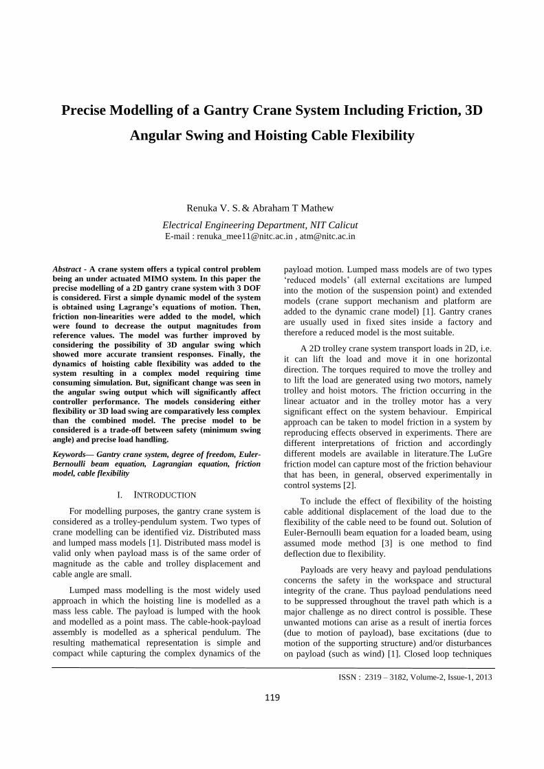
Fig 2. 2D model output without friction

The PID controlled output without friction is

obtained, as in Fig 2. The trolley displacement reached a

magnitude 1 instantaneously due to lightly damped

nature of crane and absence of friction. The cable length

magnitude initially oscillates due to the combined effect

of gravity and the controller. It finally settles to the

reference value, in about 20 seconds, due to the control

action. It is observed that angular swing is zero for zero

friction when trolley velocity is zero. Also it is noticed

that angular swing is not affected by cable length

variation in the absence of friction. Fig 3 shows the

effect of friction on the output. Due to friction the

trolley displacement and cable length are found to settle

at values below their corresponding reference values.

The swing angle is reaching up to about 5 radians

initially and also all three outputs are taking much time

to settle. Therefore a more suitable controller is

required.

Fig 3. 2D model output with friction

C. 2d Non-Linear Model With 3d Angular Swing

Fig 4 shows the swing motion of the load caused by

trolley movement of a 4DOF (x displacement of trolley,

y displacement of trolley, hoisting cable length and

angular swing) gantry crane system. The trolley and the

load are considered as point masses and are assumed to

move in a 3D plane. The trolley can move along the

girder in Y direction and the girder moves along the X

direction. Here, θx is angular swing component in x

direction (rad), θy is angular swing component in y

direction (rad), x is displacement of the girder (m), y is

displacement of trolley along girder(m), l is hoist cable

length in meters, fx is control force applied to the trolley

in the X-direction (N) , fy is control force applied to the

0 20 40 60 80 100 120 140 160 180 200-1

-0.5

0

0.5

1

t(s)

The

ta(r

ad

)

Angular swing

0 20 40 60 80 100 120 140 160 180 2000

2

4

6

t(s)

L(m

)

Hoist Length

0 20 40 60 80 100 120 140 160 180 2000

0.5

1

1.5

2

t(s)

y(m

)

Trolley displacement

0 100 200 300 400 500 600 700 800 9000

0.25

0.5

0.75

1

t(s)

y(m

)


0 100 200 300 400 500 600 700 800 9001

1.5

2

2.5

3

t(s)

L(m

)

Hoist length

0 100 200 300 400 500 600 700 800 900-1

-0.75

-0.5

-0.25

0

0.25

0.5

0.75

1

t(s)

The

ta(r

ad

)

Swing angle



122

trolley in the Y-direction (N), fl is control force applied

to the payload in the l -direction (N), mp is payload

mass(kg) and I is mass moment of inertia of the payload

(kgm2).

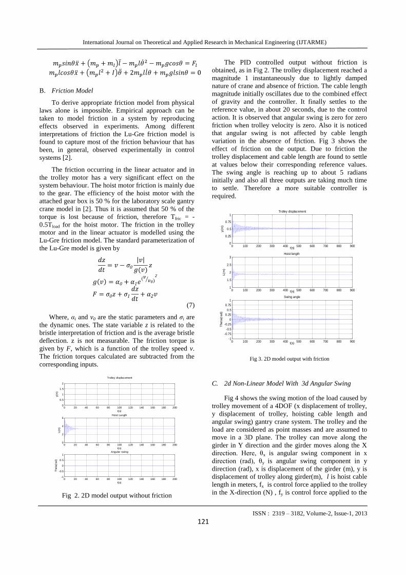
Fig 4. Trolley-cart model of 3D overhead crane [5]

The gantry crane system considered in this paper is of

3 degree of freedom having no x displacement. When

the girder is in rest and trolley is in motion, the three

dimensional crane model resembles the two-dimensional

crane model [6].Thus the girder displacement x and its

derivatives are zero. But forces in X direction can be

present in the form of disturbances acting directly on

payload and is taken as Fx. Therefore we get,

(8)

(8)

For the given system, the generalised coordinate

vector q and force vector F are given by,

(9)

(9)

Deriving the Lagrangian equations using the

above data, the dynamic equations of the system is

obtained.

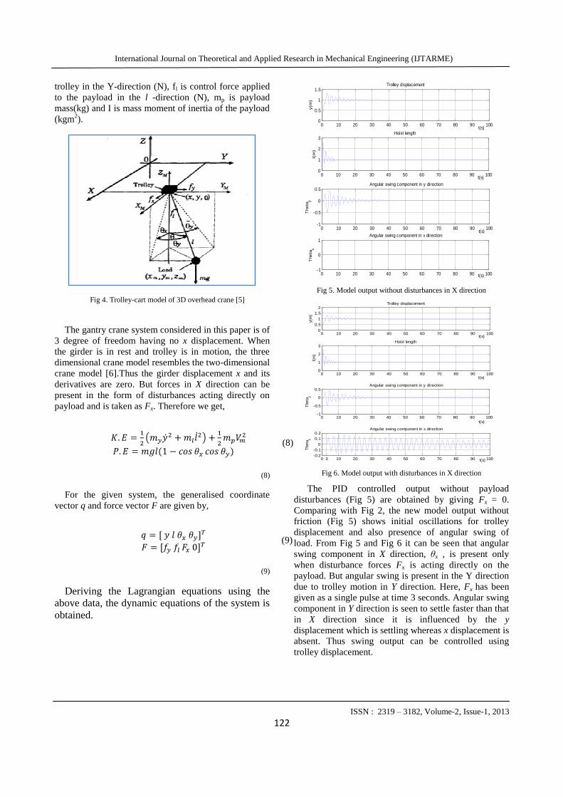
Fig 5. Model output without disturbances in X direction

Fig 6. Model output with disturbances in X direction

The PID controlled output without payload

disturbances (Fig 5) are obtained by giving Fx = 0.

Comparing with Fig 2, the new model output without

friction (Fig 5) shows initial oscillations for trolley

displacement and also presence of angular swing of

load. From Fig 5 and Fig 6 it can be seen that angular

swing component in X direction, θx , is present only

when disturbance forces Fx is acting directly on the

payload. But angular swing is present in the Y direction

due to trolley motion in Y direction. Here, Fx has been

given as a single pulse at time 3 seconds. Angular swing

component in Y direction is seen to settle faster than that

in X direction since it is influenced by the y

displacement which is settling whereas x displacement is

absent. Thus swing output can be controlled using

trolley displacement.

0 10 20 30 40 50 60 70 80 90 1000

0.5

1

1.5

t(s)

y(m

)


0 10 20 30 40 50 60 70 80 90 1000

1

2

3

t(s)

l(m

)

Hoist length

0 10 20 30 40 50 60 70 80 90 100-1

-0.5

0

0.5

t(s)

The

tay

Angular swing component in y direction

0 10 20 30 40 50 60 70 80 90 100-1

0

1

t(s)

The

tax

Angular swing component in x direction

0 10 20 30 40 50 60 70 80 90 1000

0.5

1

1.5

2

t(s)

y(m

)


0 10 20 30 40 50 60 70 80 90 1000

1

2

3

t(s)

l(m

)

Hoist length

0 10 20 30 40 50 60 70 80 90 100-1

-0.5

0

0.5

t(s)

The

tay


0 3 10 20 30 40 50 60 70 80 90 100-0.2

-0.1

0

0.1

0.2

t(s)

The

tax




123

Adding friction to the new 2D model, the trolley

displacement and hoist cable length does not reach the

reference values as observed previously. But, compared

to new model output without friction (Fig 5), output

with friction (Fig 7) shows that oscillations are taking

longer time to settle due to the combined effect of

friction and control action

Fig 7. Model output with 3D angular swing and friction

A. 2d Non-Linear Model With Load Hoisting And

Flexible Cable

Fig 8 shows the load swing in a trolley-pendulum

model of a 2D 3DOF gantry crane system with a

flexible cable. v(x,t) is the deflection of a point on the

cable at a distance x from the trolley end of cable in

meters. All the rest of the notations are the same as that

in Fig 1.Here, v is a function of x as well as time t. Then,

deflection of the cable tip is v(l,t) where l is the length of

the cable.

Fig 8. 2D gantry crane with load hoisting and flexible rod

v(l,t) can be found using the solution of Euler-

Bernoulli beam equation using assumed modes method.

In this method, deflection is expressed as a sum of two

functions: a function of displacement along the length of

the cable (Shape function∅𝑖 𝑥 ) and a function of time

(generalized co-ordinates δi(t )) [7].

From the solution of Euler-Bernoulli beam equation [8],

deflection v at a distance x along the cable is,

(5.1)

(10)

(11)

Where,

(12)

for a loaded beam [3].

The coordinates of the payload is given by,

Kinetic and potential energies of the system is given by,

(14)

If the cable is assumed to be mass-less the kinetic

energy of the cable Kcable can be neglected. For the given

system, the generalised coordinate vector q and force

vector F are given by,

q = [y l θ δ]T F=[Fy Fl 0 0]

T

(15)

Using the above equations, the dynamic equations of

the system are obtained using Lagrange‟s equation of

motion

0 10 20 30 40 50 60 70 80 90 100 110 120 130 140 1500

0.5

1

t(s)

y(m

)


0 10 20 30 40 50 60 70 80 90 100 110 120 130 140 1500

0.5

1

1.5

2

t(s)

l(m

)

Hoist Length

0 10 20 30 40 50 60 70 80 90 100 110 120 130 140 150-0.5

-0.25

0

0.25

0.5

t(s)

The

tay


0 10 20 30 40 50 60 70 80 90 100 110 120 130 140 150-1

0

1

t(s)

The

tax




124

Fig 9. 2D model open loop response without friction and cable

flexibility for 6s

Fig 10. 2D model open loop response with friction and cable flexibility for 6s (t = 0.03n)

Comparing Fig 9 and Fig 10, the effect of friction is

observed to decrease the rate of increase of trolley

displacement and hoist cable length. The effect of

flexibility is seen in angular swing of payload. The

swing angle is seen to decrease significantly compared

to the model output without considering cable

flexibility. A possible explanation to this phenomenon

can be explained with Fig 11.

Fig 11. Deflection of a flexible rope

This difference in the actual angle will be having

important implications on controller performance.

E. 3d Non-Linear Model With Load Hoisting And

Flexible Cable

It has been observed previously that the transients

are better captured by the model including 3D angular

swing dynamics. Therefore, the same derivation is

attempted here including the dynamics of cable

flexibility.

The 3D gantry crane model used before is again

considered with having a flexible cable (Fig 12). The

two components of the additional deflection due to the

flexibility of the cable v(x,t) are given by v(ly,t) and

v(lx,t).

Fig 12. 3D gantry crane with load hoisting and flexible cable

Where,

(16)

The coordinates of the payload is given by,

(17)

The kinetic and potential energies of the system will

be

(18)

0 1 2 3 4 5 60

5

10

15

20

t(s)

y(m

)


0 1 2 3 4 5 6-0.1

-0.05

-0.09

0

t(s)

The

ta(r

ad

)

Swing angle

0 1 2 3 4 5 60

50

100

150

200

t(s)

L(m

)

Length of Hoist



125

For the given system, the generalised coordinate vector

q and force vector F are given b ,

(19)

Deriving the Lagrangian equations using the above

data, the dynamic equations of the system is obtained.

The obtained model is 3D with 4 degrees of

freedom. To get 2D 3DOF model with 3D angular

swing, the girder displacement or displacement in X

direction is taken as zero, i.e. x and its derivatives are

taken as zero in the dynamic equations obtained above.

Further adding friction as the complete model is

obtained.

The simulation of the obtained model is complex

and highly time consuming. It was observed that 3D

swing angle is only present in the case of disturbances

acting directly on the load. This complex model with 3D

swing angle needs to be used only if these direct

disturbances are to be considered. Still, it was also

observed that the transients in the trolley displacement

and angular swing were shown only by this model. For

the lightly damped crane system the controller should

consider both the transient and steady state response [1].

III. CONCLUSION

A dynamic non-linear modelling of a 2D gantry

crane system with 3 DOF has been considered in this

paper. First, a 2D 3DOF gantry crane model was

obtained using Lagrangian equations of motion. Friction

non-linearities were then added to the model which was

found to decrease the output magnitudes. The model

was further improved by considering the possibility of

3D angular swing which showed more accurate transient

responses. Finally, the dynamics of hoisting cable

flexibility was added to the system resulting in a

complex model requiring time consuming simulation.

But, significant change was seen in the angular swing

output which will have important effect in controller

performance. The model without considering flexibility

is much simpler. But the significant difference in the

open loop response of the models with and without

considering cable flexibility demands the inclusion of

the dynamics of cable flexibility. The models

considering either flexibility or 3D load swing are

comparatively less complex than the combined model.

The solution lies in whether minimization of angular

swing or precise positioning of load is given higher

importance. Gantry cranes used in construction sites will

demand safety i.e. minimal angular swing rather than

precision load handling. Transportation industries

demand precision while safety aspect depends on the

work site and size of load. Manufacturing industries can

compromise on load swing if work space is not cluttered

and is fully automated.

IV. REFERENCES

[1] Eihab M.Abdel-Rahman, Ali H. Nayfeh and Ziyad N.

Masoud,”Dynamics and Control of Cranes:A Review,”

Journal of Vibration and Control, no.9,pp. 863-908,2003

[2] L.Eriksson, V.Holtta, M.Misol,”Modelling, Simulation and

Control of a Laboratory-scale Trolley-crane System”,47th

Conference on Simulation and Modelling, September 2006,Helsinki,Finland.

[3] Shihabudheen K V,” Precise Modeling And Composite

Control Of Flexible Link Flexible Joint Manipulator”, M.tech Thesis, National Institute of Technology, Calicut, India, 2012

[4] Hahn Park, Dongkyoung Chwa and Keum-Shik Hong,”A

Feedback Linearization Control of Container Cranes: Varying

Cable Length,”International Journal of Control, Automation,

and Systems, vol. 5, no. 4, pp. 379-387, August 2007

[5] Ho Hoon Li, “Modeling and Control of a Three Dimensional Overhead Crane”, Journal of Dynamic Systems, Measurement

and Control, vol.120, pp.471-476, December1998.

[6] Pramod C.P.,”Application of Adaptive Network Based Fuzzy Inference System in Control of Overhead Crane”, M.tech

Thesis, National Institute of Technology,Calicut,India,2012.

[7] K. Vishwas,”Nonlinear Modeling And End-Point Control Of Single Link Flexible Manipulator Using SDRE

Controller”,M.tech Thesis, National Institute of

Technology,Calicut,India, 2011

[8] Chung-Feng Jeffrey Kuo and Shu-Chyuarn Lin “Modal

Analysis and Control of a Rotating Euler-Bernoulli Beam Part

I: Control System Analysis and Controller Design” Mathl. Comput. Modeling Vol. 27, no. 5, pp. 75-92, 1998.

precise modelling of a gantry crane system including · pdf fileissn : 2319 – 3182,...

Documents