This content has been downloaded from IOPscience. Please scroll down to see the full text.

Download details:

IP Address: 5.219.195.77

This content was downloaded on 20/04/2016 at 19:58

Please note that terms and conditions apply.

Prediction of lung tumor motion extent through artificial neural network (ANN) using tumor size

and location data

View the table of contents for this issue, or go to the journal homepage for more

2016 Biomed. Phys. Eng. Express 2 025012

(http://iopscience.iop.org/2057-1976/2/2/025012)

Home Search Collections Journals About Contact us My IOPscience

Biomed. Phys. Eng. Express 2 (2016) 025012 doi:10.1088/2057-1976/2/2/025012

PAPER

Prediction of lung tumor motion extent through artificial neuralnetwork (ANN) using tumor size and location data

Ines-Ana Jurkovic1, Sotirios Stathakis1, Nikos Papanikolaou1 andPanayiotisMavroidis1,2

1 Department of RadiationOncology, University of TexasHealth Sciences Center SanAntonio, TX,USA2 Department of RadiationOncology, University ofNorthCarolina, ChapelHill, NC,USA

E-mail: jurkovic@livemail.uthscsa.edu

Keywords: datamining, artificial neural network, 4DCT,motion

AbstractThe aimof this study is to assess the possibility of developing novel predictivemodels based on datamining algorithmswhichwould provide an automatic tool for the calculation of the extent of lungtumormotion characterized by its known location and size. Datamining is an analytic processdesigned to explore data in search of regular patterns and relationships between variables. Theultimate goal of datamining is prediction of the future behavior. Artificial neural network (ANN)data-mining algorithmwas used to develop an automaticmodel, whichwas trained to predict extentof the tumormotion using the data set obtained from the available 4DCT imaging data. The accuracyof the designed neural networkwas tested by using longer training time, different input values and/ormore neurons in its hidden layer. An optimized ANNbestfit the training and test datasets with aregression value (R) of 0.97 andmean squared error value of 0.0039 cm2. Themaximumerror that wasrecorded for the best network performance was 0.32 cm in the craniocaudal direction. The overallprediction error was largest in this direction for 70%of the studied cases. In this study, the concepts ofneural networkswere discussed and anANNalgorithm is proposed to be usedwith clinical lung tumorinformation for the prediction of the tumormotion extent. The results of optimized ANNarepromising and can be a reliable tool formotion pattern calculation. It is an automated tool, whichmayassist radiation oncologists in defining the tumormargins needed in lung cancer radiation therapy.

1. Introduction

Currently available treatment planning systems calcu-late dose distributions on a static CT imaging set.Nevertheless, respiratory induced tumor motionresults in noteworthy movement of the tumor volumeduring the breathing cycle whichmay lead to consider-able discrepancies between the planned and delivereddose distributions (Lujan et al 1999, Chui et al 2003,George et al 2003, Naqvi and D’Souza 2005, Brandneret al 2006). This is especially a concern in the lungtumor radiotherapy due to the respiratory inducedintra-fraction motion (Cox et al 2003). Studies haveshown that tumors in the lung can move up to 3–5 cm(Shirato et al 2004, 2006). The anatomical motion issomewhat accounted for during treatment planningand delivery by using different methods andapproaches (tumor tracking, gating etc) as well as byincreasing the 3D margins to the delineated tumor.

Therefore, there is a great interest in the developmentof computational tools that will assist in the tumormargin design, offering reliable ways of reducing themwhile ensuring that the full extent of the tumor volumeis treated.

The generation of a single 4D CT scan involves adigital reconstruction of the CT slices over the respira-tory cycle. Published data (Underberg et al 2004) haveshown that individualized assessment of tumormotion can improve the accuracy of target definitionand it is best achieved by using a 4DCTdataset.

This study is inspired by our preliminary findingson the existence of a certain correlation between dif-ferent factors influencing tumor motion in the lungand the related need to develop a tool that could accu-rately predict this motion in the 3D space. Our objec-tives are twofold. First, we want to use the power of theavailable 4D CT imaging data to predict tumormotion. Until now, a lot of research has been done on

RECEIVED

7November 2015

REVISED

14March 2016

ACCEPTED FOR PUBLICATION

21March 2016

PUBLISHED

7April 2016

© 2016 IOPPublishing Ltd

this topic (Seppenwoolde et al 2002, Liu et al 2007,Boldea et al 2008, Sonke et al 2008). Most of them tryto address the respiration-induced tumor motion inthe lung by looking specifically at the tumor locationand its correlation to the extent of themotion.

Our second objective is the development of a reli-able tool by utilizing an artificial neural network(ANN) algorithm. ANNs are proven to be a valuabletool in a multitude of applications (Burke 1994,Bottaci 1997, Wei et al 2004, Dogra et al 2013, Ahmadet al 2014, Kourou et al 2015), as well as in cancer diag-nosis and prediction. In the latter case, the network isdesigned to look at pattern recognition and use it totranslate input (e.g. different biopsy attributes) andoutput (cancer categories) data. The potential useful-ness of this tool with the right set of data is significant(Konstantina Kourou 2014). Neural networks aretrained using different samples and are used in numer-ous applications; for instance in bioinformatics, opti-cal character recognition, object detection, imageprocessing, stockmarket prediction, modeling humanbehavior, loan risk analysis, pattern classification, can-cer prognostics (Burke 1994, Bottaci et al 1997, Weiet al 2004, Dogra et al 2013, Ahmad et al 2014, Kon-stantinaKourou 2014).

In this study, neural networks are used for tumormotion prediction based on the different factors thatmay be influencing its motion extent, as they wereidentified in our preliminarywork.

2.Material andmethods

2.1.DatasetThe current study was performed on the 4D CTdatasets of 11 radiotherapy patients who were treatedfor lung cancer. The dataset of each patient included12 subsets: maximum intensity projection (MIP),average intensity projection (AIP) and ten equallyspaced phases of equal duration (the breathing cyclewas sampled at ten different instances and aCTdatasetwas created for each instance). The clinical targetvolume was delineated on each set of images for eachpatient.

The reference dataset for the tumormotion assess-ment was the AIP CT. After performing a DICOMregistration for aligning each CT set with the averageCT dataset, the corresponding tumor volumes werecopied to the AIP CT, wheremotion was subsequentlydetermined by looking at their related center of themass. The same procedure was applied on theMIP CTdataset.

2.2. Artificial neural networkIn 1943, Warren S McCulloch, a neuroscientist, andWalter Pitts, a logician, developed the first theoreticalmodel of an ANN. In their paper, ‘A logical calculus ofthe ideas imminent in nervous activity’, they describethe concept of a neuron, a single cell living in a network

of cells that receives inputs, processes those inputs,and generates an output (Shiffman 2012). ANN isinspired by the structure of the brain and consists of aset of highly interconnected entities, called neurons.Each accepts a weighted set of inputs and respondswith an output, figure 1. ANN has been applied inclustering, pattern recognition, object detection,image processing, function approximation, and pre-diction systems. ANN uses several architectures andcan be trained to solve problems by using a teachingmethod and sample data. If proper training is put inplace ANN has the ability to recognize similaritiesamong different input data. As such, it represented anideal tool that can utilize similarities found in tumorsize and/or location.

One of themost commonly used ANNs is themul-tilayer perceptron (MLP). In machine learning, per-ceptron is a type of linear classifier, i.e. an algorithmfor supervised classification of an input into one ofseveral possible outputs. MLP maps set input dataonto a set of appropriate outputs and it consists ofmultiple layers of nodes with each layer being con-nected to the next one. Apart from the input nodes,each node is a neuron. MLP utilizes the back-propagation (BP) algorithm for supervised networktraining. BP algorithm is capable of handling largelearning problems as it looks for the minimum of theerror function in weight space using the method ofgradient descent. There are different variants of thisalgorithm: quasi-Newton, conjugate gradient BP, one-secant BP, Levenberg Marquardt (LM), resilient BP,and many others (Møller 1993). The designed ANNwas programmed using the neural network toolbox inMATLAB (Beale et al 2010). In MATLAB training andlearning functions are mathematical procedures usedto automatically adjust the network’s weights and bia-ses. In MATLAB’s perceptron, networks initial valuesof theweights and biases are zeros.

In this work, the LM algorithm was adopted totrain the designed ANN. The LM algorithm is a stan-dard method used to solve nonlinear least squares

Figure 1.AnANN layer of neurons.

2

Biomed. Phys. Eng. Express 2 (2016) 025012 I-A Jurkovic et al

problems. Least squares problems arise when fitting aparameterized function to a set of measured datapoints by minimizing the sum of the squares of theerrors (SSE) between the data points and the function.Nonlinear least squares problems arise when the func-tion is not linear in the parameters. Nonlinear leastsquares methods involve an iterative improvement toparameter values in order to reduce the SSE betweenthe function and the measured data points. The LMalgorithm interpolates between the following twominimization algorithms: the gradient descentmethod and the Gauss–Newton algorithm. In the gra-dient descent method, the SSE is reduced by updatingthe parameters in the direction of the greatest reduc-tion of the least squares objective. In the Gauss–New-ton algorithm, the SSE is reduced by assuming the leastsquares function is locally quadratic, and finding theminimum of the quadratic. The LM algorithm ismorerobust than the Gauss–Newton algorithm, and is avery popular curve fitting algorithm used in manysoftware applications (Gavin 2011). The main advan-tage of this algorithm is that it requires less number ofdata for training and achieves accurate results. Thenetwork training function updates weight and biasvalues according to LMoptimization.

The default network for function fitting problems,a feed forward network, with the default tan-sigmoidtransfer function in the hidden layer and linear trans-fer function in the output layer was used as this type ofnetwork can be used for any kind of input to outputmapping (Beale et al 2010). A feedforward networkwith one hidden layer and enough neurons in the hid-den layer can fit any finite input–output mapping pro-blem. The network was created with varying numberof neurons in the input layer and three neurons in theoutput layer, because there are three target values asso-ciated with each input vector. In our network design,once the training started, the number of neurons nee-ded in the hidden layer was determined experimen-tally as there is no precise rule for their selection(Othman and Ghorbel 2014). More neurons requiremore computation, and they have a tendency to overfit the data when the number is set too high, but theyallow the network to solve more complicated pro-blems. The error criterion that was used for training ismean square error (MSE), as training functions usedutilizes the Jacobian for calculations, which assumesthat performance is a mean or sum of squared errors(SSE). Therefore, networks trained with this functionmust use either theMSE or SSE performance functionand MSE is the default performance function for feedforward network. In the designed network, MSE is theaverage squared difference between output and targetvalues. The network algorithm adjusts the weights andbiases of the network so as to minimize this MSE.Another default measure used to validate the networkperformance is regression; R. R values measure thecorrelation between output and target values. An Rvalue of 1means a close relationship (Beale et al 2010).

ANN training algorithms seek to minimize errorin neural networks, however local minima can be aproblem, and this problem can be addressed by vary-ing the number of neurons in the hidden layer up untilthe acceptable accuracy is achieved. The first step wasto find the suitable number of neurons in the hiddenlayer of the ANNarchitecture.

The number of iterations (called epochs)was set tostop the training when the best generalization wasreached. This was achieved by partitioning the datainto different sub datasets: training, validation andtesting. In the ANN training, a set is used to train thenetwork while another validation set is used to mea-sure the error; network training stops when the error isincreasing for the validation dataset. Values belongingin each subset are randomly chosen and they changeon each training step (Beale et al 2010). The valuesused in a testing set have no effect on training and soprovide an independent measure of the network per-formance during and after training. The number ofneurons in the hidden layer was varied from 1 to 30and the MSE and regression values for each trial wererecorded. Each time a neural network is trained, it canresult in a different solution due to different initialweight and bias values and different divisions of datainto training, validation, and test sets. Weight and biasvalues are automatically updated according to the LMoptimization. Network default values were used fortraining parameters such as maximum number ofepochs, performance goal, maximum validation fail-ures, initial adaptive learning parameter value, etc.

Other parameters such as subset partition andnumber of variables in the input dataset were variedthrough training process and their MSE and regres-sion values were recorded in order to determine whichof the available parameters influence output, i.e. acc-uracy of the prediction, themost. The trained networkwas then used to predict motion extent for the varioussets of the tumor attributes.

2.3. ANN input datasetThe dataset used as the input was extracted from ourpreliminary study (Jurkovic et al 2016). That studycompiled tumor motion and volume change databased on the tumor size and/or location and itinvestigated their relationship patterns. In this studyfor each of the studied patients the whole respiratorymotion through the phases was divided in the twoseparate trajectories—inhale and exhale. Similaritybetween the inhalation and exhalation trajectories wasevaluated by using two different measures, dynamictimewarping and Fréchet distance, and the assessmentessentially showed that motion trajectories in theinhale and exhale phases do depend on the locationbut also depend significantly on the tumor size, i.e. itwas shown that two categories of patients have mostsimilar inhale–exhale trajectories: patients with largertumor volumes (>100 cm3) regardless of the tumor

3

Biomed. Phys. Eng. Express 2 (2016) 025012 I-A Jurkovic et al

location, and patients with tumor volumes >15 cm3

that are located in the upper lung lobe. Regressionanalysis was also performed when comparing thesimilarity between the motion paths through thewhole breathing cycle among the different patientsversus the tumor size and location in order to establishif there is any correlation. Calculated coefficient (0.73)indicated amoderate linear relationship between thesevariables. This information was subsequently appliedtowards the network design and input data extraction.The variables used were tumor volume as delineatedon the AIP CT dataset and tumor location in the lung:left/right lung, upper/middle/lower lobe, anterior/posterior location, and/or central/peripheral loca-tion, table 1.

Different subsets of the input dataset were used toestablish the best training dataset for the designed net-work and algorithm.

2.4. ANNoutput datasetRegarding the output dataset that was used fortraining, the validation and testing were based on thefindings of the preliminary study that calculated themaximum motion extents in the superior–inferior(SI), left–right (LR) and anterior–posterior (AP) direc-tions (table 2). The motion extents were calculatedusing the tumor volume center of mass (COM)positions through the ten breathing phases in relationto the COM of the tumor volume on the AIP CTdataset. This position was used as a coordinate systemcenter with coordinates 0,0,0.

Based on the foregoing analytical decisions, ANNwas designed inMATLAB and one of the resulting net-work architectures is shown in figure 2. This is a feed-forward network that has one-way connections frominput to output layers and it is one of the four availabletypes of supervised neural networks (Beale et al 2010).It is most commonly used for prediction, patternrecognition, and nonlinear function fitting.

3. Results

The best generalization was achieved by partitioningthe data into 80% training, 10% validation and 10%

testing sub datasets. Several different ANN configura-tions were initially tested with varying number ofneurons in the hidden layer. The result with the bestMSE and regression values was then used to determinethe appropriate number of neurons in the hidden layerof the ANN. We noticed that with increasing numberof neurons beyond 10we did not get any improvementinMSE andR values.

Subsequently, we further examined the networkby varying the number of variables in the input data-set. Again, the best result was achieved when all theavailable variables were taken into account. However,even when the number of variables was lowered downto two (looking only at the tumor size and location inthe lung lobes: lower, middle, upper to predict motionextent), the prediction gave a maximumMSE value of0.0099 cm2 with a regression value of 0.93. Comparedto our output data this is translated to amaximum dif-ference of −0.31 cm of the motion extent in SI direc-tion between the target data and data predicted withANN (predicted value was higher than the measuredone). The corresponding error in the LR direction was−0.17 cm and in the AP direction it was 0.15 cm(table 4). To clarify this point, sinceMSE is the averagesquared difference between all the output and targetvalues and R is regression value that measures correla-tion between all the output and target values, the

Table 1. Input dataset.

Patient# Tumor size (cm3) Lung Lobe Location 1 Location 2

1 1.66 Right Middle Anterior Central

2 11.04 Right Lower Posterior Peripheral

3 21.90 Right Upper Anterior Central

4 2.48 Right Upper Posterior Peripheral

5 108.93 Left Upper Posterior Central

6 14.11 Left Lower Posterior Central

7 29.91 Left Upper Posterior Central

8 21.70 Left Lower Posterior Central

9 96.55 Right Upper Anterior Central

10 23.47 Right Lower Posterior Central

11 17.75 Right Lower Anterior Central

Table 2.Output dataset (maximummotion extent).

Patient# LR (cm) SI (cm) AP (cm)

1 0.19 0.62 0.45

2 0.25 1.00 0.38

3 0.73 0.25 0.24

4 0.20 0.75 0.34

5 0.06 0.25 0.21

6 0.15 0.37 0.25

7 0.25 0.37 0.28

8 0.10 0.76 0.15

9 0.25 0.37 0.25

10 0.28 1.25 0.25

11 0.27 0.75 0.45

Prediction error was calculated for each of the trials

according to the following: error=desired out-

put−guessed output.

4

Biomed. Phys. Eng. Express 2 (2016) 025012 I-A Jurkovic et al

maximum differences (errors) between output andtarget values for eachmotion direction for a given net-work’s MSE and R values can be calculated based onthe following equations, (Beale et al 2010):

{ } { } { }¼p t p t p t, , , , , , ,Q Q1 1 2 2

( ( ) ( ))å= -=Q

t k n kMSE1

,k

Q

1

2

where pQ is an input to the network, tQ is thecorresponding target output, and nQ is the networkoutput. The default regression equation betweeninputs and outputs is a curve in three-dimensionalinput space. However, the plots and total regressionvalues reported are the one-dimensional regressions ofoutput versus target:

= +y bx a,

where y is the output and x is the target value, and R isthe correlation between x and y.

Furthermore, to also test the ANNwe varied num-ber of subsets that were used for training, validationand testing. The network performed best when moredata was used for training. For each run, theMSEs and

regression values were recorded. The lowest error andbest regression values, looking at the network that alsoused maximum number of input variables, wereachieved with ANN#3, MSE=0.0039 cm2 andregression value=0.971 71 (table 3). This table actu-ally shows the ANN runs that gave the best results withthe different setups after retrainingwas performed.

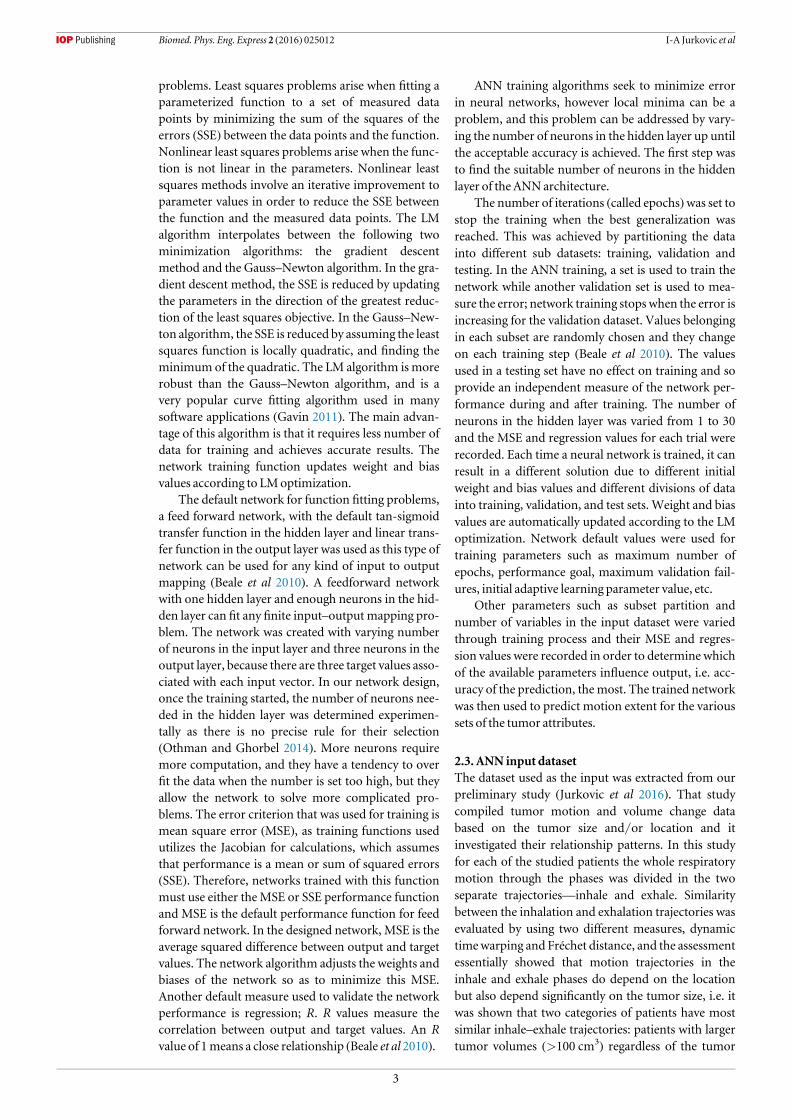
In ANN, an epoch (cycle) is a measure of the num-ber of times that all the training vectors are used toupdate the weights (network is presented with a newinput pattern). It is the number of iterations needed toachieve adequate network training, i.e. until mini-mum gradient is reached. In our case, depending onthe number of input variables, the values in the parti-tion sets and the number of neurons in the hiddenlayer, final number of epochs during training rangedfrom5 to 50 (for the runs with the lower number of theinput parameters). An example of the network perfor-mance is shown in figure 3. This figure shows whenbest validation performance is reached. Epoch 6 in thisexample indicates the iteration at which the validationperformance reached aminimum. And then the train-ing continued for a few more iterations before the

Table 3.TheANNexperimentation results for varying numbers of the partition subsets, input factors, andneurons in the hidden layer.

ANN Partition subsets Hidden layer neurons Input data MSE (cm2) Regression

1 70%, 15%, 15% 30 5 0.0391 0.846 91

2 50%, 25%, 25% 10 5 0.0207 0.849 80

3 80%, 10%, 10% 10 5 0.0039 0.971 71

4 80%, 10%, 10% 30 5 0.0051 0.963 26

5 80%, 10%, 10% 30 3 0.0335 0.740 57

6 80%, 10%, 10% 10 2 0.0099 0.928 57

7 70%, 15%, 15% 10 5 0.0108 0.932 88

8 70%, 15%, 15% 1 5 0.0241 0.827 34

9 70%, 15%, 15% 3 5 0.0223 0.843 59

10 70%, 15%, 15% 6 5 0.0106 0.927 72

11 80%, 10%, 10% 10 4 0.0071 0.954 33

12 80%, 10%, 10% 10 3 0.0067 0.951 74

13 80%, 10%, 10% 30 3 8.97E-05 0.999 17

Figure 2.Example of theMATLABANNarchitecture.

Table 4.Motion extent error values for theANNwith the two input parameters.

Direction/patient# 1 2 3 4 5 6 7 8 9 10 11

LR (cm) 0.00 0.08 0.02 −0.02 0.00 −0.06 −0.01 −0.17 0.00 −0.01 0.03

SI (cm) 0.00 0.29 0.02 −0.03 0.00 −0.31 −0.01 −0.24 0.00 0.04 0.01

AP (cm) 0.00 0.05 −0.01 0.00 0.00 −0.07 0.01 −0.11 0.00 0.01 0.15

5

Biomed. Phys. Eng. Express 2 (2016) 025012 I-A Jurkovic et al

training stopped. The figure does not indicate anymajor problems with the training. The validation andtest curves are very similar. If the test curve hadincreased significantly before the validation curveincreased, then it is possible that some overfittingmight have occurred. Generally, the error reducesafter more epochs of training, but might start toincrease on the validation data set as the network startsoverfitting the training data. In the MATLAB’s NeuralNetwork Toolbox default setup, the training stopsafter six consecutive increases in validation error, andthe best performance is taken from the epoch with thelowest validation error (Beale et al 2010).

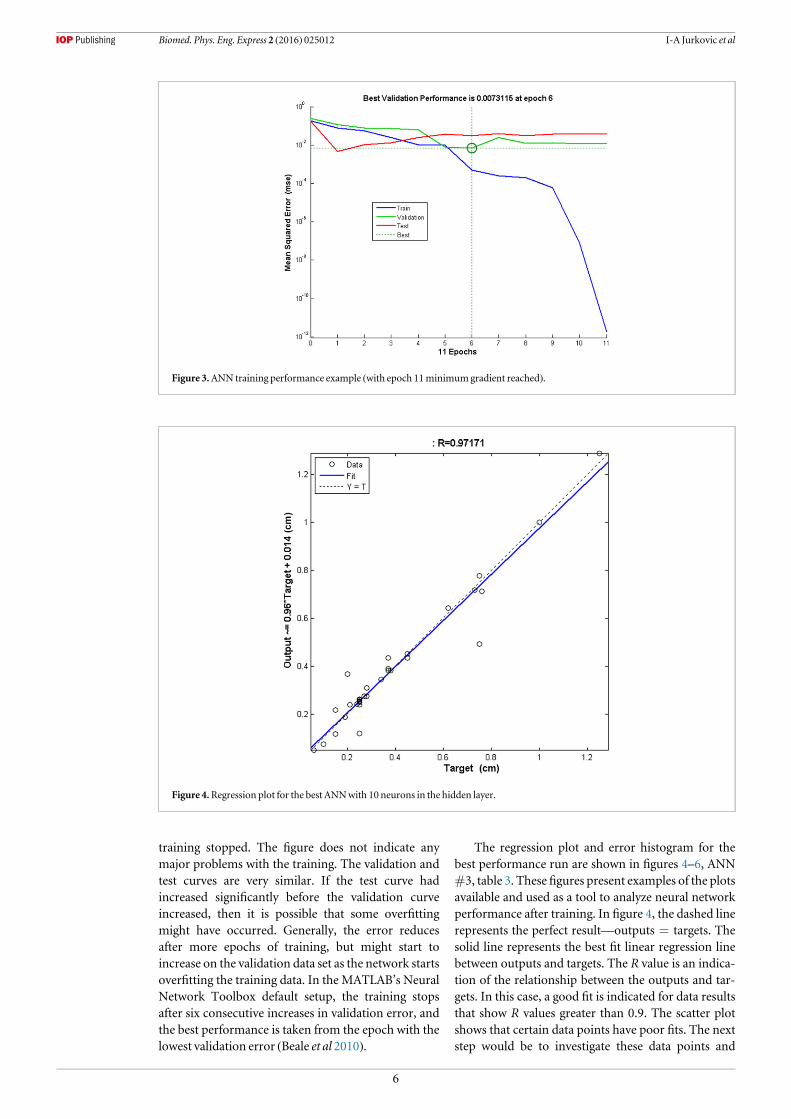
The regression plot and error histogram for thebest performance run are shown in figures 4–6, ANN#3, table 3. These figures present examples of the plotsavailable and used as a tool to analyze neural networkperformance after training. In figure 4, the dashed linerepresents the perfect result—outputs=targets. Thesolid line represents the best fit linear regression linebetween outputs and targets. The R value is an indica-tion of the relationship between the outputs and tar-gets. In this case, a good fit is indicated for data resultsthat show R values greater than 0.9. The scatter plotshows that certain data points have poor fits. The nextstep would be to investigate these data points and

Figure 3.ANN training performance example (with epoch 11minimumgradient reached).

Figure 4.Regression plot for the best ANNwith 10 neurons in the hidden layer.

6

Biomed. Phys. Eng. Express 2 (2016) 025012 I-A Jurkovic et al

determine if they should be included in the trainingset, in which case we would need additional data in thetest data set. Error histograms plotted in figures 5 and6 provide additional verification of network perfor-mance. In figure 6, the blue bars represent trainingdata, the green bars represent validation data, and thered bars represent testing data. This histogram can beused to point out outliers, which are data points wherethe fit is significantly worse than the majority of data.In this case, we notice that while most errors fallbetween −0.07 and 0.06, there is a validation pointwith an error of 0.12 and test points with errors of−0.16 and 0.25. These outliers are also visible on theregression plot, figure 4. We can check the outliers todetermine if the data is bad, or if those data points aredifferent than the rest of the data set. If the outliers arevalid data points, but are unlike the rest of the data,then the network is extrapolating for these points.

Next step would be to collect more data that looks likethe outlier points, and retrain the network, i.e. have alarger data set for training and testing of a neural net-work. Same reasoning applies to a data plotted in thefigures 7 through 9. As shown in table 3, the 5th ANNhad three input variables, which were chosen for thenetwork design (tumor size, upper/lower lung andanterior/posterior location). The 6th ANN had twoinput variables chosen for the network design (tumorsize and upper/lower lung location). Finally, the 11thANN had four input variables chosen for the networkdesign (tumor size, left/right lung, upper/lower lung,and peripheral/central tumor location). In all thecases, when the regression values for all the subsetswere>0.8 and the MSE values<0.005 cm2, retrainingwould stop. This was achievable for all the ANNsexcept for the one that had 30 neurons in the hiddenlayer and three input variables (number 5). However,

Figure 5.Error histogramplot for the best ANNwith 10 neurons in the hidden layer.

Figure 6.Error histogramplot for the best ANNwith 10 neurons in the hidden layer, with the partitions also shown.

7

Biomed. Phys. Eng. Express 2 (2016) 025012 I-A Jurkovic et al

when the network was further retrained we achieveda MSE value of 8.97E-05 cm2 and a regressionvalue of 0.9992 (ANN number 13 in table 3), whichis also shown in figures 7–9. This is probably due toover-fitting and/or larger training subset, whichrequires more test data to be used for additionalchecks.

Table 5 shows the error values obtained from thebest network result with the 10 neurons in the hiddenlayer. The maximum errors were −0.17 cm in the LRdirection, 0.26 cm in the SI direction and−0.07 cm inthe AP direction. In 70% of the cases, the maximumerror was in the craniocaudal direction, mostly

because tumor motion values in that direction had awidest span of values for the examined cases.

4.Discussion

Our preliminary work (Jurkovic et al 2016) showedthat there is a preferred tumor motion direction (left,inferior, regardless of the location), more specifically,upper/middle tumors move predominantly left(67%), anterior (67%) and inferior (83%), while lowerlesions tend to move more left (60%), posterior (60%)and inferior (60%). Overall, for all the cases, displace-ment was predominantly left (64%), anterior (55%)

Figure 7.Regression plot for the best ANNwith 30 neurons in the hidden layer after excessive retraining.

Figure 8.Error histogramplot for the best ANNwith 30 neurons in the hidden layer after excessive retraining.

8

Biomed. Phys. Eng. Express 2 (2016) 025012 I-A Jurkovic et al

and inferior (73%). This was confirmed by the largestvolume change in those directions (Jurkovicet al 2016), where for each patient, tumor volumeresiduals (FUS (volume that is sum of all tumorvolumes through the breathing phases)—AIP (volumedelineated on the AIP CT dataset)) were calculated foreach of the plane halves. The results show that in themajority of the cases the FUS residual volume partprevailed on the following directions: left, 82%,posterior, 55%, and inferior, 64%. The preferredtumor motion that was observed relates to the motionof the tumor volume COM in the AIP CT datasetagainst the COM in each phase CT dataset. Morespecifically, it was found that smaller volume sizesrequire contouring on all the phases since contouringonly on the AIP and MIP scans will not cover theextent of motion and volume change in these cases. Inother clinical cases, it was found that there is 3D anglesimilarity when plane fitting is done that depends onthe tumor size and location and this can allow foradequate margin calculation when certain parametersare known without extra contouring on all the phases;for example it was found that the lower located tumorshave AP angles around 30° and LR-AP angles around50° and more specifically in all the studied examplescorrelation was found between the best line fit and thetumor location. In most instances the R2 value wasgreater than 0.9 for those planes. Hysteresis (thedifference between the inhalation and exhalation

trajectory of the tumor) is studied in various publica-tions (Seppenwoolde et al 2002, Mageras et al 2004,Low et al 2005, Boldea et al 2008,White et al 2013) andrepresents an important issue for the patients withlung cancer. In most studies computing hysteresisbetween the trajectories came to calculating themaximum distance between inhalation polygonalcurve and exhalation polygonal curve, which can bedone by using different distance measures, i.e. Frechetdistance for example. In our study we used similarapproach and found that there is correlation betweenthe motion trajectories among individual patientsdepending on the tumor size and location and alsobetween the inhale and exhale paths in some patientsthat allows for contouring on either just the inhale orexhale phase (Jurkovic et al 2016). This finding maylead to a reduction of the work labor especially forsmaller tumors where contouring on all the phases isrecommended.

Taking into account these findings, the correlationthat is found between various factors was furtherexplored, and used as a basis for the neural networkcreation and design.

Once trained, ANN performed well with regres-sion values that included all three subsets (training,validation and test), which were above 0.80 in almostall cases regardless of the number of input parameterschosen. Some studies point out that a neural networkmay be an unstable predictor or classifier as it may

Figure 9.Error histogramplot for the best ANNwith 30 neurons in the hidden layer with the partitions also shown.

Table 5.Motion extent error values for the best ANN in cm.

Direction/

patient# 1 2 3 4 5 6 7 8 9 10 11 Average

LR 0.00 0.00 0.01 −0.17 0.01 0.03 0.13 0.03 0.00 0.00 0.00 0.005

SI −0.02 0.00 0.00 0.26 0.01 −0.02 −0.07 0.05 −0.01 −0.04 −0.03 0.012

AP 0.00 0.00 0.00 −0.01 −0.03 −0.01 −0.03 −0.07 0.01 −0.01 0.02 −0.012

9

Biomed. Phys. Eng. Express 2 (2016) 025012 I-A Jurkovic et al

have high error in the test datasets due to the over fit-ting on the training dataset (i.e. small changes in initialconditions can lead to high variability in predictions).To overcome this problem amethod for reducing var-iance is suggested. This method is called bagging,which works best with unstable models but candegrade performance of the stable models (Brei-man 1998). Bagging is performed using a bootstrapmodel where bootstrap samples of a training set usingsampling with replacement are created. Each boot-strap sample is used to train a different component ofbase classifier. However, our network showed goodperformance even with the test datasets, constantlyachieving regression values above 0.80 andMSE valuesbelow 0.005 cm2 when all the input parameters wereused for the network design.

In MATLAB’s default network setup (MATLAB &Simulink. n.d.) each network is trained starting fromdifferent initial weights and biases, andwith a differentdivision of the first dataset into training, validation,and test sets. Note that the test sets are a goodmeasureof generalization for each respective network, but notfor all the networks, because data that is a test set forone network will likely be used for training or valida-tion by other neural network runs. This is why it isrecommended to divide the original dataset into twoparts, to ensure that a completely independent test setis preserved. However, in the case of a limited sizedataset this is not possible. As a consequence, witheach run, data is divided randomly and differently foreach setup leading to different results, i.e. MSE and Rvalues. For each of the setups multiple runs are per-formed and then the one with the best overall perfor-mance is chosen, which does not necessarilymean thatdue to the fact that different divisions among datawereapplied we do not run into overfitting in some of theruns. In our case, we did not have an independentdataset to further check the network’s behavior. Wealso followed these rules to assess the reasonability ofthe results: the final MSE is small and the test set errorand the validation set error have similar characteristics(figure 3). If the network performance is not satisfac-tory it is recommended to increase the number of hid-den neurons and/or increase the number of inputvalues.

Another problem is overgeneralization (MATLAB& Simulink. n.d.). The purpose of training a feedfor-ward network is to modify weight values iterativelysuch that the weights, ultimately, converge on a solu-tion that correctly relates inputs to outputs. It is nor-mally desirable during the training of a network to beable to generalize basic relations between inputs andoutputs based on training data, which may not consistof all possible inputs and outputs for a given problem.A problem that can arise in the training of a neural net-work involves the tuning of weight values so closely tothe training data that the usefulness of the network inprocessing new data is diminished, which results in

over-generalization (or over-training). Basically, thismeans that the network training may incorporate fea-tures of the training dataset that are uncharacteristic ofthe data as a whole. However, as the measured errorcontinually decreases, the network usefulness and cap-abilities will also be decreasing (as the network modi-fies weights to match the characteristics of the trainingdata). This is also where validation and test sets comeinto the picture, since the network’s MSE and R valuesare a result of the whole network’s behavior, i.e. eventhough theMSE values that are result of the validationand tests dataset may be lower, the overall MSE value(due to the high training set MSE value) may be highenough for the network run to pass our criteria.

Nevertheless, we need to point out limits of ourapproach. The data set used was small and by increas-ing the number of neurons in such limited data set sizewe run into the issue of over fitting. In order toimprove the results of the motion extent predictiondesigned network, the dataset size should be increased.The inclusion of the larger datasets would also givemore accurate and stable results. An issue to be dis-cussed concerns the number of hidden neurons usedduring each trial. However, multiple published studies(Elisseeff and Paugam-Moisy 1996, Lawrenceet al 1998, Basheer andHajmeer 2000, Priddy and Kel-ler 2005, Devaraj et al 2007, Kuncheva 2012, Sheelaet al 2013, Mozer et al 2014) show that in most of thecases several rules of thumb are suggested, but themost popular approach for finding the optimal num-ber of hidden nodes is by trial and error with one of thementioned rules as starting point, i.e. retrain the net-work with varying numbers of hidden neurons andobserve the output error as a function of the numberof hidden neurons. Furthermore, a study done byTetko et al (1995) states that real examples suggest arather wide tolerance of ANN to the number of thehidden layer neurons. From our study it is apparentthat even with the limited size of the presented dataset,a solution with acceptable accuracy could be found.Once network is build and trained, the results can beused for the adequatemargin design.

The amount of the input data can be as large asneeded and/or deemed necessary. We have shownthat we can achieve good results with only two inputneurons, but this is most probably due to the fact thatfor a particular run the training dataset was much lar-ger than the validation and testing datasets, andthe network may have simply over fit the data,which emphasizes our conclusion of more casesneeded to test network’s stability and accuracy.Besides the data that was already taken into account,tumor characteristics can be further stratified toinclude pathology, tumor stage, attachment to rigidstructures, simulation setup (compression being usedor not), etc.

10

Biomed. Phys. Eng. Express 2 (2016) 025012 I-A Jurkovic et al

5. Conclusions

The present study discussed the concepts related toneural networks and proposes the use of a given ANNalgorithm together with the clinical lung tumorinformation for prediction of the tumor motionextent. Based on the analysis of our results theproposed solution has several advantages—automatedmotion extent prediction using the ANN algorithm,usage of the readily available clinical data, and possiblehigh prediction accuracy. In the future, we aim atincorporating more clinical tumor information withthe application of different algorithms on the pro-posed platform, use a larger data set, and carry outadditional studies to further improve their liability andstability of the proposed neural network.

Acknowledgments

Author Ines-Ana Jurkovic, Author Sotirios Stathakis,Author Nikos Papanikolaou, and Author PanayiotisMavroidis declare that they have no conflict of interest.This research received no specific grant from anyfunding agency in the public, commercial, or not forprofit sectors.

References

Ahmad F, RoyK,O’Connor B, Shelton J, Dozier G andDworkin I2014 Flywing biometrics usingmodified local binary pattern,SVMs and random forest Int. J.Mach. Learn.Comput. 4279–85

Basheer I A andHajmeerM2000Artificial neural networks:fundamentals, computing, design, and applicationJ.Microbiol.Methods 43 3–31

BealeMH,HaganMT andDemuthHB2010 Neural NetworkToolbox 7User’s Guide,MathWorks

BoldeaV, SharpGC, Jiang S B and SarrutD 2008 4D-CT lungmotion estimationwith deformable registration:quantification ofmotion nonlinearity and hysteresisMed.Phys. 35 1008–18

Bottaci L, DrewP J,Hartley J E,HadfieldMB, FaroukR, Lee PW,Macintyre IM,DuthieG S andMonson J R 1997Artificialneural networks applied to outcome prediction for colorectalcancer patients in separate institutions Lancet 350 469–72

Brandner ED,WuA, ChenH,HeronD,Kalnicki S, Komanduri K,GersztenK, Burton S, Ahmed I and ShouZ 2006Abdominalorganmotionmeasured using 4DCT Int. J. Radiat. Oncol.Biol. Phys. 65 554–60

Breiman L 1998Arcing Classifiers Ann. Stat. 26 801–24BurkeHB1994Artificial neural networks for cancer research:

outcome prediction Semin. Surg. Oncol. 10 73–9ChuiC-S, Yorke E andHong L 2003The effects of intra-fraction

organmotion on the delivery of intensity-modulated fieldwith amultileaf collimatorMed. Phys. 30 1736–46

Cox JD, SchechterNR, Lee AK, Forster K, Stevens CW,AngK-K,Komaki R, Liao Z andMilas L 2003Uncertainties in physicaland biological targetingwith radiation therapyRays 28 211–5

Devaraj D, Roselyn J P andRani RU2007Artificial neural networkmodel for voltage security based contingency rankingAppl.Soft Comput. 7 722–7

DograHK,Hasan Z andDogra AK 2013 Face expressionrecognition using scaled-conjugate gradient back-propagation algorithm Int. J.Mod. Eng. Res. 3 1919–22

Elisseeff A and Paugam-MoisyH1996 Size ofMultilayer Networks forExact Learning: Analytic Approach (EcoleNormaleSupérieurede Lyon. Laboratoire de l’Informatique du Parallélisme [LIP])

GavinHenri P 2011The Levenberg-Marquardtmethod fornonlinear least squares curve-fitting problems (http://people.duke.edu/∼hpgavin/ce281/lm.pdf)

George R, Keall P J, Kini VR,VedamS S, Siebers J V,WuQ,LauterbachMH, ArthurDWandMohanR 2003Quantifying the effect of intrafractionmotion during breastIMRTplanning and dose deliveryMed. Phys. 30 552–62

Jurkovic I-A, PapanikolaouN, Stathakis S, Li Y, Patel A,Vincent J andMavroidis P 2016Assessment of lung tumourmotion and volume size dependencies using variousevaluationmeasures J.Med. Imaging Radiat. Sci. in press(doi:10.1016/j.jmir.2015.11.003)

KourouK, Exarchos T P, Exarchos KP, KaramouzisMVandFotiadisD I 2015Machine learning applications in cancerprognosis and predictionComput. Struct. Biotechnol. J. 138–17

Kuncheva L 2000 Fuzzy Classifier Design (Berlin: Physica-Verlag)Lawrence S, Giles C L andTsoi AC 1998What SizeNeuralNetwork

GivesOptimal Generalization? Convergence Properties ofBackpropagationOnline: http://drum.lib.umd.edu/handle/1903/809

LiuHH et al 2007Assessing respiration-induced tumormotion andinternal target volume using four-dimensional computedtomography for radiotherapy of lung cancer Int. J. Radiat.Oncol. Biol. Phys. 68 531–40

LowDA, Parikh P J, LuW,Dempsey J F,Wahab SH,Hubenschmidt J P,NystromMM,HandokoMandBradley JD 2005Novel breathingmotionmodel forradiotherapy Int. J. Radiat. Oncol. Biol. Phys. 63 921–9

LujanAE, Larsen EW, Balter JMandHakenRKT1999Amethodfor incorporating organmotion due to breathing into 3Ddose calculationsMed. Phys. 26 715–20

MagerasG S et al 2004Measurement of lung tumormotion usingrespiration-correlated CT Int. J. Radiat. Oncol. Biol. Phys. 60933–41

MATLAB&Simulink. n.d. ImproveNeural NetworkGeneralization andAvoidOverfitting (http://mathworks.com/help/nnet/ug/improve-neural-networkgeneralization-and-avoid-overfitting.html)

MøllerMF 1993A scaled conjugate gradient algorithm for fastsupervised learningNeural Netw. 6 525–33

MozerMC, Smolensky P, TouretzkyD S, Elman J L andWeigendA S 2014Proc. 1993ConnectionistModels SummerSchool (Oxford: Psychology Press)

Naqvi SA andD’SouzaWD2005A stochastic convolution/superpositionmethodwith isocenter sampling to evaluateintrafractionmotion effects in IMRTMed. Phys. 32 1156–63

Othman I B andGhorbel F 2014 Stability evaluation of neural andstatistical classifiers based onmodified semi-bounded plug-inalgorithm Int. J. Neural Netw. Adv. Appl. 1 37–42

PriddyKL andKeller P E 2005Artificial Neural Networks(Bellingham,WA: SPIE)

Seppenwoolde Y, ShiratoH,Kitamura K, Shimizu S, vanHerkM,Lebesque J V andMiyasakaK 2002 Precise and real-timemeasurement of 3D tumormotion in lung due to breathingand heartbeat,measured during radiotherapy Int. J. Radiat.Oncol. Biol. Phys. 53 822–34

Sheela KG,Deepa SN, Sheela KG andDeepa SN2013Review onmethods to fix number of hidden neurons in neural networksMath. Probl. Eng. 2013 e425740

ShiffmanD2012TheNature of Code: SimulatingNatural Systemswith Processing (TheNature of Code)

ShiratoH, Seppenwoolde Y, Kitamura K,Onimura R and Shimizu S2004 Intrafractional tumormotion: lung and liver Semin.Radiat. Oncol. 14 10–8

ShiratoH et al 2006 Speed and amplitude of lung tumormotionprecisely detected in four-dimensional setup and in real-timetumor-tracking radiotherapy Int. J. Radiat. Oncol. Biol. Phys.64 1229–36

11

Biomed. Phys. Eng. Express 2 (2016) 025012 I-A Jurkovic et al

Sonke J-J, Lebesque J and vanHerkM2008Variability of four-dimensional computed tomography patientmodels Int. J.Radiat. Oncol. Biol. Phys. 70 590–8

Tetko IV, LivingstoneD J and Luik A I 1995Neural network studies:I. Comparison of overfitting and overtraining J. Chem. Inf.Comput. Sci. 35 826–33

Underberg RWM, Lagerwaard F J, Cuijpers J P, SlotmanB J,van Sörnsen deKoste J R and Senan S 2004 Four-dimensionalCT scans for treatment planning in stereotactic radiotherapy

for stage I lung cancer Int. J. Radiat. Oncol. Biol. Phys. 601283–90

Wei J S et al 2004 Prediction of clinical outcome usinggene expression profiling and artificial neuralnetworks for patients with neuroblastomaCancer Res. 646883–91

White B, ZhaoT, Lamb J,Wuenschel S, Bradley J, ElNaqa I andLowD2013Distribution of lung tissue hysteresis during freebreathingMed. Phys. 40 043501

12

Biomed. Phys. Eng. Express 2 (2016) 025012 I-A Jurkovic et al