pressure transmission model for well drilling operations c…

Proceedings of COBEM 2011 21st Brazilian Congress of Mechanical Engineering Copyright © 2011 by ABCM October 24-28, 2011, Natal, RN, Brazil

PRESSURE TRANSMISSION MODEL FOR WELL DRILLING OPERATIONS

Gabriel Merhy de Oliveira, [email protected] Admilson Teixeira Franco, [email protected] Cezar O. R. Negrão, [email protected] Thermal Science Laboratory (LACIT) Post-graduate Program in Mechanical and Materials Engineering (PPGEM), Federal University of Technology - Parana (UTFPR) – Av. Sete de Setembro, 3165, CEP 80.230-901 – Curitiba-PR-Brazil Abstract. During well drilling, the pressure within the wellbore may become too small and an influx of formation fluid may come into the well. This is called kick and may have two different causes: i) the drilling fluid weight is two low to hold the fluid in the formation or ii) the drillstring or casing motion lowers the wellbore pressure below the formation pressure. Although the kick can be detected by changes of pressure within the wellbore pressure is only measured while drilling and also a small influx of gas does not change significantly the bottomhole pressure. Another indication of kick is the change of pressure at the wellhead, but this is usually only detected when a large amount of gas has entered the well. Besides, some drilling fluids do not transmit pressure as expected – the magnitude of the measured pressure is smaller than the predicted. The current work presents a compressible transient flow model to predict pressure transmission within the wellbore. The model comprises the conservation equations of mass and momentum which are solved by the method of characteristics. Drilling fluids are admitted to work as Non-Newtonian Bingham fluids and the viscous effect is modeled by employing a friction factor approach. The model results were compared to some experimental values for a Newtonian (water) and two drilling fluids. Not only the magnitudes but also the oscillation frequencies of measured and computed values agree quite well for water and drilling fluids. On the contrary to the Newtonian fluid, both measured and computed values of pressures for Bingham fluids do not stabilize uniformly along the well after pressurization. In other words, the predicted and measured pressures are not completely transmitted for Bingham fluids. Keywords: Drilling fluid, Bingham fluid, compressible flow, transient simulation

1. INTRODUCTION

In oil well drilling, an important task is the control of the bottomhole pressure within a narrow range. Nowadays, the downhole pressure is controlled by balancing the hydrostatic pressure of the drilling fluid and the formation pressure. Whenever the bottomhole pressure becomes smaller than the formation pressure there is a risk of the formation fluid (oil, natural gas and/or water) to come into the wellbore and up to the annulus (the space between the drill string and the walls of the open hole). The influx of the formation fluid is called kick and if it is not controlled the kick can escalate to a blowout (the uncontrolled release of crude oil and/or gas from an oil well after pressure control systems have failed) when the formation fluid reaches the surface, especially in case of gas influx. Therefore, a small inflow of gas should be detected as soon as possible. Nevertheless, the pressure is only measured while drilling and also a small influx of gas cannot change significantly the bottomhole pressure. Another indication of kick is the change of pressure at the wellhead which is only noticed when a large amount of gas has come into the well. It has been advocated by the industry that some drilling fluids do not transmit pressure as expected. In other words, the pressure applied at a certain point in the well is not perceived at the magnitude it is expected in another position in the wellbore.

Mathematical modeling is not only important for predictions of fluid flows and process alike but also to help the understanding of physical phenomena. Some works in the literature have been dedicated to the modeling of the start-up flows (Sestak et al., 1987, Cawkwell and Charles, 1987, Chang et al., 1999 and Davidson et al., 2004, Oliveira et al. 2010) which is similar to the problem described above. In start-up flows, a pressure step change is imposed at a pipe inlet and the pressure travels along the pipe length before the fluid starts to flow. This is quite similar to what takes place in well pressure transmission.

Most of the above works study the restart of waxy crude oils at low temperatures. The work of Sestak et al. (1987), Cawkwell and Charles (1987), Chang et al. (1999) and Davidson et al. (2004) consider that a gelified waxy crude fills completely a pipeline and it is displaced by a non-gelified oil. Chang et al. (1999) and Sestak et al. (1987) disregard the transient effects in the momentum conservation equations and admit equilibrium of pressure difference and wall shear stress forces at any time. The time variation of pressure occurs only due to changes of the rheology properties which are time-dependent. Despite been an updated version of the Chang´s et al. (1999) paper, Davidson et al. (2004) only added compressibility to the fluid but they still did not consider the transient terms of the governing equations. On the other hand, Cawkwell and Charles (1987) have not taken into account the advective terms of the momentum equation but had included the transient terms into their analysis. Vinay et al. (2006) presented a 2-D transient model to simulate the compressible start-up flow of a Bingham fluid. In a second work, Vinay et al. (2007) put forward a 1-D model and compared the results with their 2-D model. In spite of the good agreement, they concluded that the 1-D model is much

Proceedings of COBEM 2011 21st Brazilian Congress of Mechanical Engineering Copyright © 2011 by ABCM October 24-28, 2011, Natal, RN, Brazil faster to run, reducing the computing time from hours and days to seconds and minutes. In a recent work, Wachs et al. (2009) developed what they called a 1.5D model in which they conflate their 1-D model to the 2-D one.

It is worthy of noting that all the above works usually use the finite difference method or a variation of it to solve the equations. However, Wylie et al. (1993) have advocated that the computation time can be considerably reduced if the Method of Characteristics (MOC) is used to solve one-dimensional problems.

The current work puts forward a mathematical model to simulate the pressure transmission problem described above. The geometry consists of a pipe (the drillstring) connected to the annular space formed between the drill pipe and the wellbore. The flow is considered to be isothermal, one-dimensional and compressible. The wall shear rate is computed by using the friction factor for Newtonian and Bingham fluids. The equations are solved by the Method of Characteristics that converts partial differential equations into ordinary ones to solve them iteratively. The model is then applied to simulate tests performed in an experimental plant of Petrobras, located in São Sebastião do Passé – BA (NUEX-Taquipe). 2. MATHEMATICAL MODEL 2.1. Problem Description

Figure 1a shows a schematic representation of the drilling operation at the wellbore bottom in which a drilling fluid is pumped into the drill pipe. The fluid flows through the drill bit roles and then returns by the annular space carrying the cuttings. While drilling, the bottomhole pressure must be kept within an operational rage (window) in order to avoid the influx of formation fluids and the fracture of the rock formation.

Despite the changes of the cross sectional areas of the drill pipe and annular space, the geometry will be simplified as a constant cross sectional pipe (drill pipe) and annular space, as shown in Figure 1b. According to Figure 1c, the drill pipe internal diameter is identified as D and the internal and external diameters of the annular space as D1 and D2, respectively. The region below the drill pipe is disregarded in the modeling and the fluid is considered to flow directly from the drill pipe to the annular space, as the drill bit is not considered to be in place. The flow in both drill pipe and annular space is admitted to be compressible, isothermal and one-dimensional in the axial direction. Besides, the drill pipe and the well structure are admitted to be completely rigid and therefore, do not deform. The shear stress at the pipe walls (drill pipe and annular space) is evaluated by employing the concept of friction factor and the drilling fluid is dealt as a Bingham fluid.

Figure 1. (a) Illustration of the drilling fluid circulation in the wellbore. (b) Longitudinal view and (c) cross section of drill pipe and annular space

2.2 Governing Equations

For weakly compressible flows such as those found in drilling operations, the non-linear terms V zρ∂ ∂ and

V V zρ ∂ ∂ can be disregarded in the mass and momentum conservation equations, respectively. By applying the hypotheses mentioned in the previous section and by employing a constant compressibility approach, the conservation equations of mass and momentum can be written as,


2 0Vct zρ ρ∂ ∂+ =

∂ ∂ (1)

21 0h

f V VV Pt z Dρ

∂ ∂+ + =

∂ ∂ (2)

where ρ , V and P are the average values of density, velocity and pressure across the cross sectional area and c is the pressure wave speed. f is the Fanning friction factor which depends on the geometry (pipe or annular space) and fluid properties (Newtonian and Bingham fluid). t is the time and z is the axial position. hD is the hydraulic diameter, which is defined as 2 1D D− for the annular space and D for the pipe.

2.3 Constitutive Equation and Friction Factor

The drilling fluid is considered to behave as a Bingham fluid and its constitutive equation is written as,

0τ τ ηγ= + (3)

where τ is the shear stress, γ is the shear rate, 0τ is the yield stress and η is the plastic viscosity. This correlation is implicitly used to calculate the friction factor.

The friction factor depends on the fluid properties and the domain under analysis. For laminar flows, Fanning friction factor can be written as (Fontenot and Clark, 1974):

,

16Rez t

f ζλ

= (4)

where ζ is geometric parameter which is 1.0 for pipe flow and 1.5 for a narrow annular flow ( 1 2 0.5D D ≥ ), λ is the fluid conductance of the Bingham fluid and ,Rez t is the Reynolds number that depends on time and on the position along the domain ( ,Rez t hVDρ η= ). Equations (5) and (6) are the correlations used to calculate the fluid conductance for the pipe and annular space, respectively,

4

, ,

, ,

He He116Re 3 8Re

P z t P z tP

z t z t

λ λλ

⎛ ⎞= − + ⎜ ⎟⎜ ⎟

⎝ ⎠ (5)

3

, ,

, ,

He He118Re 2 12Re

A z t A z tA

z t z t

λ λλ

⎛ ⎞= − + ⎜ ⎟⎜ ⎟

⎝ ⎠ (6)

where ,Hez t is the Hedstrom number ( 2 2, 0Hez t hDρτ η= ) which depends on time and space. The subscripts P and A

are the pipe and annular space, respectively. Equation (4) can be reduced to the Newtonian friction factor if the Hedstrom number (or yield stress) is made equal to zero.

According to Fontenot and Clark (1974), the Bingham fluid flow can be considered to be laminar if ,Re 2000z tγ ≤ , otherwise is turbulent. For the cases shown in the results section, only Bingham laminar flows are investigated. For Newtonian fluid flows, on the other hand, both laminar and turbulent flows are taken into account. The turbulent Newtonian flow is admitted to take place if ,Re 2100z t > and the turbulent friction factor adopted is one suggested in White (2003):

0.25, ,0.079Re , Re 2000turb z t z tf −= > (7)

2.4 Solution of the Equations

The governing equations are solved by the method of characteristics (MOC), as described by Wylie et al. (1993).

The method of characteristics is a technique for solving, typically, first-order partial differential equations. The method consists on the reduction of a partial differential equation to a family of ordinary differential equations along which the solution can be integrated from some initial data given. In the current case, equations (1) and (2) are reduced to a single ordinary differential equation which is solved by the finite difference method. In comparison to the ordinary finite volume method that is usually employed on the solution of this kind of equations, the number of grid points that provides accurate results can be considerably reduced.


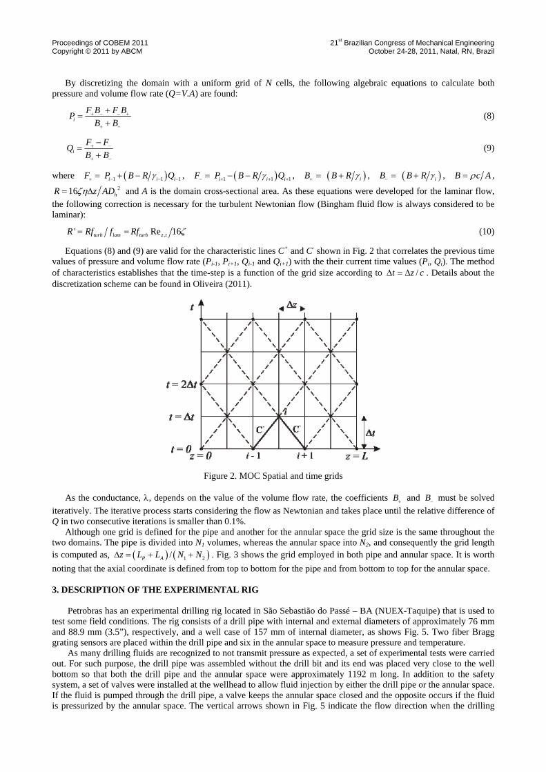
By discretizing the domain with a uniform grid of N cells, the following algebraic equations to calculate both pressure and volume flow rate (Q=V.A) are found:

iF B F BP

B B+ − − +

+ −

+=

+ (8)

iF FQB B+ −

+ −

−=

+ (9)

where ( )1 1 1 i i iF P B R Qγ+ − − −= + − , ( )1 1 1 i i iF P B R Qγ− + + += − − , ( ) iB B R γ+ = + , ( ) iB B R γ− = + , B c Aρ= , 216 hR z ADζη= Δ and A is the domain cross-sectional area. As these equations were developed for the laminar flow,

the following correction is necessary for the turbulent Newtonian flow (Bingham fluid flow is always considered to be laminar):

,' Re 16turb lam turb z tR Rf f Rf ζ= = (10)

Equations (8) and (9) are valid for the characteristic lines C+ and C- shown in Fig. 2 that correlates the previous time values of pressure and volume flow rate (Pi-1, Pi+1, Qi-1 and Qi+1) with the their current time values (Pi, Qi). The method of characteristics establishes that the time-step is a function of the grid size according to /t z cΔ = Δ . Details about the discretization scheme can be found in Oliveira (2011).

Figure 2. MOC Spatial and time grids As the conductance, λ, depends on the value of the volume flow rate, the coefficients B+ and B− must be solved

iteratively. The iterative process starts considering the flow as Newtonian and takes place until the relative difference of Q in two consecutive iterations is smaller than 0.1%.

Although one grid is defined for the pipe and another for the annular space the grid size is the same throughout the two domains. The pipe is divided into N1 volumes, whereas the annular space into N2, and consequently the grid length is computed as, ( ) ( )1 2/P Az L L N NΔ = + + . Fig. 3 shows the grid employed in both pipe and annular space. It is worth noting that the axial coordinate is defined from top to bottom for the pipe and from bottom to top for the annular space.

3. DESCRIPTION OF THE EXPERIMENTAL RIG

Petrobras has an experimental drilling rig located in São Sebastião do Passé – BA (NUEX-Taquipe) that is used to

test some field conditions. The rig consists of a drill pipe with internal and external diameters of approximately 76 mm and 88.9 mm (3.5”), respectively, and a well case of 157 mm of internal diameter, as shows Fig. 5. Two fiber Bragg grating sensors are placed within the drill pipe and six in the annular space to measure pressure and temperature.

As many drilling fluids are recognized to not transmit pressure as expected, a set of experimental tests were carried out. For such purpose, the drill pipe was assembled without the drill bit and its end was placed very close to the well bottom so that both the drill pipe and the annular space were approximately 1192 m long. In addition to the safety system, a set of valves were installed at the wellhead to allow fluid injection by either the drill pipe or the annular space. If the fluid is pumped through the drill pipe, a valve keeps the annular space closed and the opposite occurs if the fluid is pressurized by the annular space. The vertical arrows shown in Fig. 5 indicate the flow direction when the drilling


fluid is pumped through the drillpipe. The drilling fluid was either pumped by the circulation system of the rig or by a cementation unit adapted for such purpose. The circulation systems were connected to the wellhead through a high pressure pipe and they both controls the pump flow rate and maximum pressure at the pump outlet. The maximum pressure was established according to the fluid weight, as the botomhole pressure cannot surmount 27.6MPa (4000 psi). To measure the data, an acquisition system compatible with the fiber Bragg technology was used with an acquisition rate of 1000 Hz.

Figure 3. Grid distribution in the drill pipe and annular space

Figure 4. Schematic representation of the experimental rig

The results of only three sensors were used in the comparison with computed values and they are indicated in Fig. 5 (S1, S2 and S3). The first was located within the drill pipe and the last two were placed in the annular space at 29 m (S1), 1192 m (S2) and 14.64 m (S3) below the wellhead, respectively.

The tests were conducted according to the following: i) first of all, the well was filled with drilling fluid and closed; ii) the fluid was then pumped into the well with a constant flow rate until the bottomhole pressure reached 27.6 MPa (4000 psi) (maximum working pressure); iii) the pumped was then turned off and the well was kept closed until the pressure stabilized; iv) finally, the well was depressurized by the choke. In the current work, two nominal flow rates were considered: 1.325 l/s (0.5 bpm) and 9.275 l/s (3.5 bpm). In fact, the flow rate was quite difficult to control and its value varied during the experiment.

The tests were run for several fluids and only three were used in the comparison: water and two drilling fluids (fluid A and B). The fluid A has low weight and low viscosity, whereas fluid B has high weight and high viscosity. The rheology properties of fluids A and B were obtained from a Fann 35A viscometer and fitted to the Bingham model. Their wave speeds were estimated by using the time for pressure propagation between two sensors and the distance they

S3

S2

S1

Drillpipe

Well case

Blowout preveter

Proceedings of COBEM 2011 21st Brazilian Congress of Mechanical Engineering Copyright © 2011 by ABCM October 24-28, 2011, Natal, RN, Brazil are placed apart. The water properties were obtained from the literature (White, 2003). The plastic viscosity (viscosity for the water case), the yield stress, the wave speed and the density of the fluids are shown in Table 1.

Table 1. Fluids properties.

Property Water Fluid A Fluid B η [Pa.s] 0.001 0.0235 0.0677

0τ [Pa] 0 2.166 10.88

c [m/s] 1350 1000 1011

ρ [ kg/m3] 1000 1150 1929

4. MODEL SET-UP

In order to evaluate the pressure transmission throughout the well, the drilling fluid which rests in the pipe and in the annular space was suddenly pressurized by the pump. As an initial condition, the fluid was considered to stand still within the domain and consequently, the velocity/volumetric flow rate was null throughout the domain, ( , 0) 0Q z t = = . The initial pressure condition was considered to be the hydrostatic one. For the reason that a valve was always closed at the choke ( ( , 0) 0p aQ z L L t= + = = ), the flow rate is set to zero as the outlet boundary condition. As the fluid is injected into the well with the outlet valve closed, the pressure within the well increased continuously until a pre-defined pressure value, setP , was reached and the pump was then turned off. To accomplish such situation in the simulation, the following boundary condition is established at the well inlet:

( ) ( )( )

if 0, 0,

0 if 0,in set

set

Q P z t PQ z t

P z t P⎧ = <⎪= = ⎨ = ≥⎪⎩

(11)

As the pump flow rate was not precisely measured and the experimental tests were conducted mainly to evaluate the pressure transmission after the pump shut down, the pump flow rate was adjusted to fit the calculated pressure to the measured pressure at the first sensor (S1). A grid of 328 volumes was used in all simulations. 5. RESULTS

Four set of experimental data were chosen to be compared with the model results. The first two were conducted with two water flow rates, whereas the other two with two different drilling fluids.

5.1 Water

For the first water flow, the pump was turned on with a constant flow rate of 1.122 l/s (0.42 bpm) and was turned off

when the pressure at well inlet is 14.69 MPa (2130 psi). Figs. 5 and 6 show comparisons of computed and measured values of pressure in the first (located at the drill pipe inlet) and the third sensor (placed closed to the choke), respectively. The good agreement of the pressures during the first 150s in Fig. 5 cannot be taken into account, as the flow rate was imposed to make them as close as possible. After the pump has been turned off and the flow rate was made equal to zero, the agreement remained reasonable as the measured value and its counterpart oscillates at the same frequency and their amplitude are quite close. It is worth of noting that the oscillation is due to the pressure reflections at the domain boundaries and that the frequency coincides with the wave speed multiplied by the length of the domain. However, the computed and measured values start to move away from each other soon after that, as the oscillation of the measured pressure is dissipated much faster than the computed one. On the other hand, the pressure agreement in Fig. 6 is quite reasonable during the pressure rising and soon after the pump is turned off. Despite the similar format of the oscillations, the measured values still dissipate faster than the calculate ones.


t (s)

P(M

Pa)

0 50 100 150 200 250 3000

2

4

6

8

10

12

14

16

S1 - expS1 - num

150 155 160 16514

14.2

14.4

14.6

14.8

15

15.2

280 285 290 295 300

14.6

14.8

15

0 5 10 15 200

0.5

1

1.5

2

Figure 5. Time evolution of measured and computed values of pressure at position S1 for a flow water of 1.122 l/s

t (s)

P(M

Pa)

0 50 100 150 200 250 3000

2

4

6

8

10

12

14

16

S3 - expS3 - num

150 155 160 16514

14.2

14.4

14.6

14.8

15

15.2

0 5 10 15 200

0.5

1

1.5

2

280 285 290 295 300

14.6

14.8

15


t (s)

P(M

Pa)

0 20 40 60 80 100 120 140 160 1800

5

10

15

20

S1 - expS1 - num

20 25 30 35 40

12

14

16

18



t (s)

P(M

Pa)

0 20 40 60 80 100 120 140 160 1800

5

10

15

20

S3 - expS3 - num

20 25 30 35 40

12

14

16

18

Figure 8. Time evolution of measured and computed values of pressure at position S3 for a flow water of 8.7 l/s.

For the second case of water flow, the imposed flow rate changed linearly from zero to a maximum value (8.7l/s - 3.3bpm) in 8s and then was kept constant until a pressure of 15.2 MPa (2204 psi) was reached at well inlet, when the pump was then turned off. Figs. 7 and 8 show comparisons of measured and computed values of pressure at positions S1 and S3, respectively. For this higher pressure flow, the agreement is even better than that observed in Figs. 5 and 6. 4.2 Drilling Fluids

Similar tests were conducted for two drilling fluids, fluids A and B. For fluid A, the flow rate was set to the

constant value of 1.462 l/s (0.55bpm) until the pressure at well inlet achieved 13.82 MPa (2004 psi) and the pump was switched off. Figs. 9a, 9b and 9c show the time change of measured and computed values of pressure for each sensor. On the contrary to what was shown in the above figures, the pressures do not oscillate as much as that of the Newtonian fluid and this response can be noted in both computed and measured curves. This behavior can be explained by the existence of the yield stress of Bingham fluids. As soon as the pump is turned off, the pressure starts to reflect back and forward at the boundaries and the pressure gradient begins to reduce within the domain. Whenever the pressure gradient along the domain reduces and is not able to overcome the yield stress, the pressure does not reflect anymore and then stabilizes. Although the measured and computed curves have similar responses the computed values stabilize slightly first. Differently from the Newtonian fluid whose pressure is uniform along the domain after the equilibrium (if the hydrostatic pressure is subtracted), the pressure for Bingham fluid stabilizes in different values for each domain position. One can see that the stable value of the outlet pressure is larger than the inlet one, for both measured and computed curves. In fact, both measured and computed pressure values do not became stable but they continue to change.

t (s)

P(M

Pa)

0 50 100 150 200 250 300 3500

5

10

15S1 - expS1 - num

165 170 175 18013

13.2

13.4

13.6

13.8

14

t (s)

P(M

Pa)

0 50 100 150 200 250 300 3500

5

10

15S2 - expS2 - num

165 170 175 18013

13.2

13.4

13.6

13.8

14

a) b)


t (s)

P(M

Pa)

0 50 100 150 200 250 300 3500

5

10

15S3 - expS3 - num

165 170 175 18013

13.2

13.4

13.6

13.8

14

Figure 9. Time evolution of measured and computed values of pressure for fluid A at (a) S1, (b) S2 and (c) S3 positions

The fluid B results are now discussed. The flow rate, in this case, was set to the constant value of 0.952 l/s

(0.359bpm) and the pump was turned off when the well inlet pressure reaches 7.6 MPa (1102 psi). Comparisons of the measured and computed values are shown in Fig. 10. Not only the measured and computed values are very similar again, but also they do not oscillate, as noted in fluid A results. The S1 and S2 pressures reduce suddenly after the peak and then stabilize. Despite the deviation of the measured and computed pressures during the pump up period, their values at S3 position respond very similarly, as they both reach a maximum and then become constant. The absence of oscillation in this case is due to the high apparent viscosity of this drilling fluid which dissipates the pressure wave faster in comparison to the previous case.

t (s)

P(M

Pa)

0 50 100 150 200 2500

2

4

6

8

S1 - expS2 - expS3 - expS1 - numS2 - numS3 - num

60 65 70 75 80 85 906

6.5

7

7.5

8

Figure 10. Time evolution of measured and computed values of pressure for fluid B 5. CONCLUSIONS

The current work puts forward a mathematical model to predict pressure transmission in well drilling operations. The model is based on the conservation equations of mass and momentum for a compressible, transient and one-dimensional flow. The drilling fluid is modeled as a Bingham fluid and the viscous effect is taken into account by employing the friction factor concept. The governing equations (conservation of mass, momentum and an equation of state) are solved by the Method of Characteristics. The results are compared to measured data obtained for water and two drilling fluids in an experimental rig of Petrobras. The fluid is pumped into the closed well until the pressure has reached a pre-defined value and then the pump is turned off for pressure stabilization. Good agreements between

c)

Proceedings of COBEM 2011 21st Brazilian Congress of Mechanical Engineering Copyright © 2011 by ABCM October 24-28, 2011, Natal, RN, Brazil measured and computed values are found. For the water case, not only the measured and computed pressures increase at the same rate but also they oscillate at the same frequency soon after the pump shut down. After that, the measured and computed values start to deviate from each other as the measured oscillations are dissipated faster than the computed counterparts. For Bingham fluids, nevertheless, the comparison is even better once the measured and computed values do not oscillate much. It was also noted that the oscillations diminish with the increase of the fluid yield stress. This is observed in both measured and computed values. The computed results show that the yield stress is the responsible for the oscillation dampness that takes place with drilling fluids. As soon as the pressure gradient is not enough to overcome the fluid yield stress, the oscillation stops and the pressure seems to stabilize within the domain. In fact, the pressure along the domain is not uniform as noted with Newtonian fluids and a small pressure gradient is observed. In addition, it was noted that the inlet and outlet pressures do not stabilizes completely along the domain but tend to approach each other. 6. ACKNOWLEDGEMENTS

The authors would like to thank PETROBRAS S/A, ANP (Brazilian National Oil Agency) and CNPq (The Brazilian National Council for Scientific and Technological Development) for their financial support to the work. Besides, we are particularly in dept to Eng. Rodrigo Silva of PETROBRAS S/A who had conducted the experimental tests and provided the measured data to the work. 7. REFERENCES Cawkwell, M.G. and Charles, M.E.,1987, “An Improved Model for Start-up of Pipelines Containing Gelled Crude Oil”,

J. of Pipelines, Vol. 7, pp. 41-52. Chang, C., Rønningsen, H.P. and Nguyen, Q.D.,1999, “Isothermal Start-up of Pipeline Transporting Waxy Crude Oil”,

J. of Non-Newtonian F. Mechanics, Vol. 87, pp. 127-154. Davidson, M.R., Nguyen, Q.D., Chang,C. and Ronningsten, H.P.,2004, “A Model for Restart of a Pipeline with

Compressible Gelled Waxy Crude Oil”, J. of Non-Newtonian F. Mechanics, Vol. 123, pp. 269-280. Fontenot, J.E. and Clark, R.K.,1974, “An Improved Method for Calculating Swab and Surge Pressures and Circulating

Pressures in a Drilling Well”, Soc. of Petroleum Eng. J. (SPE 4521), Vol. 14, No 5, pp 451-462. Oliveira, G. M., Rocha, L. L. V.; Franco, A. T.; Negrão, C. O. R., 2010, “Numerical Simulation of the Start-up of

Bingham fluid Flows in Pipelines”, J. of Non-Newtonian F. Mechanics, Vol. 165, pp. 1114-1128. Oliveira, G. M., 2011, Dissertação de Mestrado, Universidade Tecnológica Federal do Paraná, Curitiba-PR. Sestak, J., Cawkwell, M.G., Charles, M.E. and Houskas, M.,1987, “Start-up of Gelled Crude Oil Pipelines”, J. of

Pipelines, Vol. 6, pp. 15-24. Vinay, G., Wachs, A. and Agassant, J.F.,2006, “Numerical Simulation of Weakly Compressible Bingham Flows: The

Restart of Pipeline Flows of Waxy Crude Oils”, J. of Non-Newtonian F. Mechanics, Vol. 136, No. 2-3, pp. 93-105. Vinay, G., Wachs, A. and Frigaard, I., 2007, “Start-up Transients and Efficient Computation of Isothermal Waxy Crude

Oil Flows”, J. of Non-Newtonian Fluid Mechanics, Vol. 143, pp. 141-156. Wachs, A., Vinay, G., and Frigaard, I. 2009, “A 1.5D Numerical Model for the Start Up of Weakly Compressible Flow

of a Viscoplastic and Thixotropic Fluid in Pipelines”. J. of Non-Newtonian F. Mechanics,Vol. 159, pp. 81-94. White, F. M., 2003, Fluid Mechanics. 5th ed. New York, United States: McGraw-Hill, 866 p. Wylie, E. B., Streeter, V. L., and Suo, L., 1993, “Fluid Transients in Systems”, Ed. P. Hall, N. Jersey, U. States, 463 p. 8. RESPONSIBILITY NOTICE

The authors are the only responsible for the printed material included in this paper.

pressure transmission model for well drilling operations c…

Documents