pricing of foreign currency options in the serbian … · pricing of foreign currency options in...

91

COMMUNICATIONS

Irena Janković* DOI:10.2298/EKA0980091J

PRICING OF FOREIGN CURRENCY OPTIONS IN THE SERBIAN MARKET

* Faculty of Economics, University of Belgrade

ABSTRACT: The main idea of this paper is to find the most suitable approach to the valuation of foreign currency options in the Serbian financial market. Volatility analysis included the application of the GARCH model which resulted in the marginal volatility measure, which was used in the pricing of basic foreign currency options in

the local market. The analysis is completed with an overview of the implementation of FX derivatives in the Serbian financial market.

KEY WORDS: option pricing, stochastic volatility, GARCH model

JEL CLASSIFICATION: B23, C32, F31, G12

ECONOMIC ANNALS, Volume LIV, No. 180, January – March 2009UDC: 3.33 ISSN: 0013-3264

92

Irena Janković

1. Introduction

The work presented focuses on finding the most suitable approach to the valuation of foreign currency (FX) options in the Serbian market. The analysis includes the fitting of the GARCH specification for the RSD/EUR exchange rate return series and the implementation of the gained volatility measure in the pricing of FX options in the local market. While providing analysis we take into account local circumstances including the still underdeveloped financial market without standardized financial derivatives.

2. The Valuation of Options

An option is a financial instrument that gives the right to buy or sell an underlying asset, within a specified period of time at a specified price called the exercise or strike price. The price the buyer of the option pays in order to gain the stated right is called the option premium. An American option can be exercised at any time up to the date the option expires. A European option can be exercised only on a specified future date. The last date on which the option may be exercised is called the expiration or maturity date. Options are used as valuable tools in numerous hedging strategies as they define the price at which underlying assets can be bought or sold in the future.

Foreign currency options offer the right to buy or sell a quantity of foreign currency for a specified amount of domestic currency in the predefined period or on a specified date in the future. They provide payoffs that depend on the difference between the exercise price and the exchange rate at maturity. These options can be used as a valuable tool in hedging FX exposure.

The Black and Scholes formula - BS (Black and Scholes, 1973) for option pricing is a function of the parameters of the diffusion process describing the dynamics of the underlying asset price. The no-arbitrage principle states that if options are correctly priced in the market it should not be possible to make a guaranteed profit by creating portfolios of long and short positions in options and their underlying assets. By respecting this principle they derived a theoretical valuation formula for European options on common stocks.

C0 = S0 N(d1) – Xe-rT N(d2) (1)

P0 = Xe-rT N(-d2) - S0 N(-d1) ) (2)

PRICING OF FOREIGN CURRENCY OPTIONS IN SERBIA

93

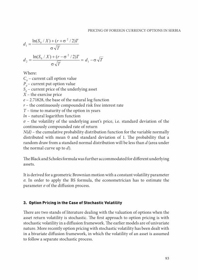
Where:C0 – current call option valueP0 – current put option valueS0 – current price of the underlying assetX – the exercise pricee – 2.71828, the base of the natural log functionr – the continuously compounded risk free interest rateT – time to maturity of the option in yearsln – natural logarithm functionσ – the volatility of the underlying asset’s price, i.e. standard deviation of the continuously compounded rate of returnN(d) – the cumulative probability distribution function for the variable normally distributed with mean 0 and standard deviation of 1. The probability that a random draw from a standard normal distribution will be less than d (area under the normal curve up to d).

The Black and Scholes formula was further accommodated for different underlying assets.

It is derived for a geometric Brownian motion with a constant volatility parameter σ. In order to apply the BS formula, the econometrician has to estimate the parameter σ of the diffusion process.

3. Option Pricing in the Case of Stochastic Volatility

There are two stands of literature dealing with the valuation of options when the asset return volatility is stochastic. The first approach to option pricing is with stochastic volatility in a diffusion framework. The earlier models are of univariate nature. More recently option pricing with stochastic volatility has been dealt with in a bivariate diffusion framework, in which the volatility of an asset is assumed to follow a separate stochastic process.

94

Irena Janković

Hull and White (1987) studied option pricing in the case of stochastic volatility where σ2 follows an independent geometric Brownian motion process from the stock price process. Provided that increments of the volatility process are independent of the increments of the process governing the asset price, they showed that options can be priced by averaging the BS formula over the stochastic volatility, i.e. the option price is the BS price integrated over the distribution of the mean volatility and there is no need to price the risk attached to the stochastic volatility.

Noh, Engle and Kane (1994) predict the future mean volatility using a GARCH model (Bollerslev, 1986) on the past returns and plug it into the BS formula. They conclude that the GARCH estimated volatility has more economic content than the volatility estimates (implied volatility) obtained by inverting the BS formula using observed past option prices.

The BS formula, however, ignores the stochastic nature of volatility as, for instance, it is modeled by the GARCH model. It assumes homoskedasticity when the real governing process is heteroskedastic. If we want to get prices by using the BS formula we have to plug into the formula the marginal variance of the empirical GARCH process. It must be taken into account that the BS formula under prices out-of-the money options, options on low-volatility securities, and short maturity options. Also, when there is large uncertainty on marginal measures due to near nonstationarity, plugging in the BS formula can be dangerous and give dubious results. Therefore this formula has to be used with caution regarding input data and time horizons under consideration.

The second stand of literature develops the option pricing model in the GARCH framework. During the past decade researchers have begun to study generalized autoregressive conditional heteroskedastic (GARCH) models for option pricing because of their superior performances in describing asset returns.

The particular type of non-linear model that is used in finance is known as the autoregressive conditionally heteroscedastic - ARCH model (Engle, 1982). In the context of financial time series, where it is unlikely that the variance of the error terms will be constant over time, it is used as the model which describes how the variance of the error terms evolves. It is employed commonly in modeling financial time series that exhibit time-varying volatility clustering, the tendency of large changes in asset prices to follow large changes and small changes to follow small changes.


95

Under the ARCH(q) model, the conditional mean equation could take almost any form that the researcher likes, e.g.:

yt = β1 + β2x2t + β3x3t + β4x4t + … + ut (3)

ut ~ N(0, σ2t)

where yt is the variable dependent on the vector of explanatory variables xt, whose elements may be lagged values of dependent variable yt, while ut is the standard error of the model and σt is the conditional variance of the error term.

The variance of the residuals depends on past history and we face heteroskedasticity because the variance is changing over time. One way to deal with this is to have the variance depending on the lagged period of the squared error terms.

The conditional variance of the error term, σ 2t, depends on q lags of squared error

terms:

(4)

Since the ARCH model had problems deciding the value of the number of lags of the squared residual in the model q, model robustness, and conditional variance non-negativity constraint violation, it was extended through generalized ARCH, i.e. the GARCH model which is widely used in practice.

The GARCH model allows the conditional variance to be dependent upon its own previous lags. In the GARCH (p,q) model conditional variance is dependant upon q lags of the squared error term and p lags of the conditional variance.

(5)

In general, a GARCH(1,1) model is sufficient to capture the volatility clustering in the data and is most often used in financial theory and practice.

(6)

Duan (1995) provides a general method for option pricing in the case of the GARCH processes. He uses the GARCH-M model of Engle, Lilien and Robins (1987), which combines nicely with the properties of the lognormal distribution.

96

Irena Janković

The GARCH-in-mean (GARCH-M) model follows most models used in finance that assume that investors should be rewarded for taking additional risk by obtaining a higher return. One way to show this is to let the investment return be partly determined by investment risk. The GARCH-M model allows the conditional variance of asset returns to enter into the conditional mean equation. It can be presented in the following simple GARCH (1, 1)-M form:

(7)

The δ can be interpreted as a risk premium. If δ is positive and statistically significant, then increased risk caused by an increase in the conditional variance leads to a rise in the mean return.

The GARCH option pricing theory has also been extended to pricing currency-related derivative products. Empirically Duan (1996), Heston and Nandy (2000), Hardle and Hafner (2000), Hsieh and Ritchken (2005), and Christoffersen and Jacobs (2004) (among others) have shown that the GARCH model can be used to capture the pricing behaviour of exchange-traded European options.

The two mentioned stands of option pricing under stochastic volatility are unified by a convergence result of Nelson (1990) and Duan (1996).

Duan and Wei (1999) generalized the GARCH option pricing methodology in Duan (1995) to a two-country setting. Specifically, they assumed a bivariate nonlinear asymmetric GARCH model for the exchange rate and the foreign asset price, and generalized the local risk-neutral valuation principle in Duan (1995). They derived the equilibrium GARCH processes for the exchange rate and the foreign asset price in the two-country economy. Foreign currency options and cross-currency options can then be valued using the well-known risk-neutral valuation technique. This setup allows rich empirical regularities such as stochastic volatility, fat tails, and the so-called leverage effect. They also ran simulations to price quanto options1 and found that when the true environment is GARCH, in most cases a constant variance model is not reliable. The proposed equilibrium valuation framework to price foreign currency and cross-currency options is the first of its kind in the literature.

1 Quantos are options that allow the investor to fix in advance the exchange rate at which an investment in a foreign currency can be converted back to the domestic currency. The amount of the currency that will be converted depends on the investment performance of the foreign security.


97

The second stand of literature will not be our focus for now because of the still underdeveloped and illiquid local financial market and nonexistence of exchange traded FX option contracts.

The following section refers to the analysis of Serbian exchange rates and FX option pricing possibilities in the local circumstances. We model exchange rate volatility behavior by implementing the GARCH model. Then we use the gained volatility measure in the Black-Scholes formula in order to price plain vanilla FX options.

4. Analysis

The analysis that follows is focused on the nominal RSD/EUR exchange rate, formed in the local market. Volatility analysis includes fitting of the GARCH specification which results in a marginal volatility measure that can be plugged into the BS formula in order to get the prices of basic FX options.

As previously mentioned empirical works state, the combination of the GARCH specification and the BS formula should be used with caution. However this approach can be suitable in giving us the prices of theoretical FX options and guiding the introduction of these instruments in the local market. This could be very useful for their further implementation in different FX hedging strategies.

It has also been previously stated that GARCH estimated volatility has more economic content than the volatility estimates (implied volatility) obtained by inverting the BS formula using observed past option prices. The second approach still cannot be implemented because there is no historical data on FX option prices in the Serbian market and there are no such instruments present yet.

5. Data and Modeling

The sample includes daily data in the form of the natural logarithm (ln), excluding weekends and holidays, of the average nominal exchange rate RSD/EUR2, obtained for the period 3 January 2003 to 26 March 2007, comprising 1066 data points.3

2 Data is obtained from the National Bank of Serbia3 Modeling was done using the econometric software package EViews

98

Irena Janković

Figure 1. Average Daily Nominal RSD/EUR Exchange Rate (3 Jan 2003 – 26 Mar 2007)

We tested for the series stationarity and found that the series is not stationary, which is supported by the estimates of the autocorrelation and partial autocorrelation functions together with the unit-root test presented below.

Table 1. CorrelogramSample: 1 1066

Included observations: 1066Autocorrelation Partial Correlation AC PAC Q-Stat Prob

.|******** .|******** 1 0.998 0.998 1064.3 0.000

.|******** .| | 2 0.995 -0.036 2124.5 0.000

.|******** .| | 3 0.993 -0.003 3180.7 0.000

.|******** .| | 4 0.991 0.024 4233.1 0.000

.|******** .| | 5 0.989 0.008 5281.7 0.000

.|******** .| | 6 0.986 -0.004 6326.6 0.000

.|******** .| | 7 0.984 0.007 7367.9 0.000

.|******** .| | 8 0.982 0.010 8405.6 0.000

.|******** .| | 9 0.980 0.002 9439.8 0.000

.|******** .| | 10 0.978 -0.004 10470. 0.000

.|******** .| | 11 0.976 -0.006 11497. 0.000

.|*******| .| | 12 0.973 -0.001 12521. 0.000


99

Autocorrelation coefficients are statistically significant on the significance level of 5% if they are beyond the interval (±0.06).

The correlogram showed that the ACF is long exponentially decaying and that we probably have a unit root in the series and autocorrelation. By performing the unit root test on the series ln(EUR) we found that the ADF test statistic (0.432931) is higher than the critical value at a 5% significance level (-3.414066), indicating that we do not reject the null hypothesis, e.g. that there is a unit root in the series.

In order to eliminate the unit root we found the first difference in ln(EUR), i.e. exchange rate returns, ln(EUR)-ln(EUR(-1)), and did the test again.

Figure 2. First Difference of the RSD/EUR Average Nominal Exchange Rate (Returns)

Table 2. CorrelogramSample: 1 1066

Included observations: 1065Autocorrelation Partial Correlation AC PAC Q-Stat Prob

.|** | .|** | 1 0.254 0.254 69.125 0.000 .| | *| | 2 0.007 -0.062 69.178 0.000 *| | *| | 3 -0.110 -0.104 82.213 0.000

100

Irena Janković

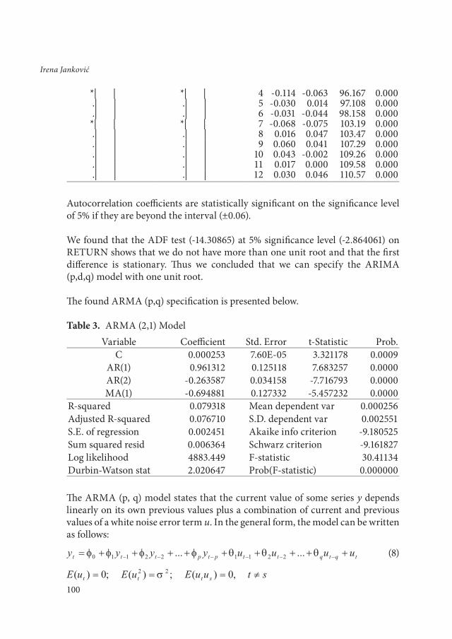
*| | *| | 4 -0.114 -0.063 96.167 0.000 .| | .| | 5 -0.030 0.014 97.108 0.000 .| | .| | 6 -0.031 -0.044 98.158 0.000 *| | *| | 7 -0.068 -0.075 103.19 0.000 .| | .| | 8 0.016 0.047 103.47 0.000 .| | .| | 9 0.060 0.041 107.29 0.000 .| | .| | 10 0.043 -0.002 109.26 0.000 .| | .| | 11 0.017 0.000 109.58 0.000 .| | .| | 12 0.030 0.046 110.57 0.000

Autocorrelation coefficients are statistically significant on the significance level of 5% if they are beyond the interval (±0.06).

We found that the ADF test (-14.30865) at 5% significance level (-2.864061) on RETURN shows that we do not have more than one unit root and that the first difference is stationary. Thus we concluded that we can specify the ARIMA (p,d,q) model with one unit root.

The found ARMA (p,q) specification is presented below.

Table 3. ARMA (2,1) ModelVariable Coefficient Std. Error t-Statistic Prob.

C 0.000253 7.60E-05 3.321178 0.0009AR(1) 0.961312 0.125118 7.683257 0.0000AR(2) -0.263587 0.034158 -7.716793 0.0000MA(1) -0.694881 0.127332 -5.457232 0.0000

R-squared 0.079318 Mean dependent var 0.000256Adjusted R-squared 0.076710 S.D. dependent var 0.002551S.E. of regression 0.002451 Akaike info criterion -9.180525Sum squared resid 0.006364 Schwarz criterion -9.161827Log likelihood 4883.449 F-statistic 30.41134Durbin-Watson stat 2.020647 Prob(F-statistic) 0.000000

The ARMA (p, q) model states that the current value of some series y depends linearly on its own previous values plus a combination of current and previous values of a white noise error term u. In the general form, the model can be written as follows:

(8)


101

Our model for exchange rate returns is ARMA (2, 1):

(9)

The correlogram did not show significant autocorrelation. The distribution of residuals indicated high kurtosis (8.057) and skewness close to zero (-0.36) with Jarque-Bera higher than 5.99.

Figure 3. Distribution of the Residuals

Since series ln(EUR) has 1 unit root and its first difference (RETURN) can be estimated with the ARMA(2, 1) model, the series ln(EUR) can be estimated with the ARIMA (2, 1, 1) model.

The analysis continued with a test for an ARCH effect presence in the specified model ARIMA (2,1,1). First we looked at the mean equation and saw that it is statistically significant. We further checked for the presence of an ARCH effect. In order to do that we looked at the correlogram of residuals squared that showed the presence of the ARCH effect. We saw that residuals are not normally distributed and that there is an ARCH effect, but in order to confirm this we performed the ARCH LM Test.

102

Irena Janković

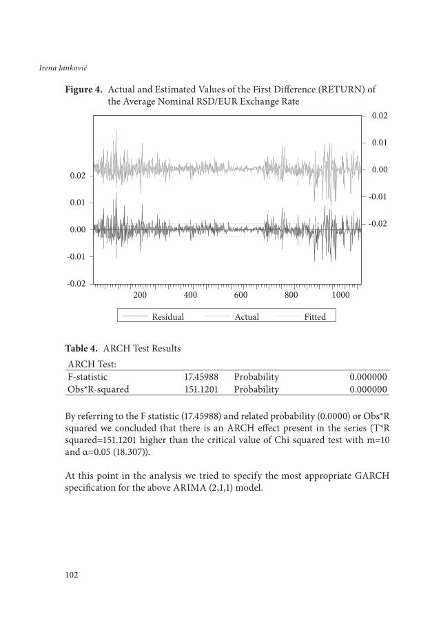
Figure 4. Actual and Estimated Values of the First Difference (RETURN) of the Average Nominal RSD/EUR Exchange Rate

Table 4. ARCH Test ResultsARCH Test:F-statistic 17.45988 Probability 0.000000Obs*R-squared 151.1201 Probability 0.000000

By referring to the F statistic (17.45988) and related probability (0.0000) or Obs*R squared we concluded that there is an ARCH effect present in the series (T*R squared=151.1201 higher than the critical value of Chi squared test with m=10 and α=0.05 (18.307)).

At this point in the analysis we tried to specify the most appropriate GARCH specification for the above ARIMA (2,1,1) model.


103

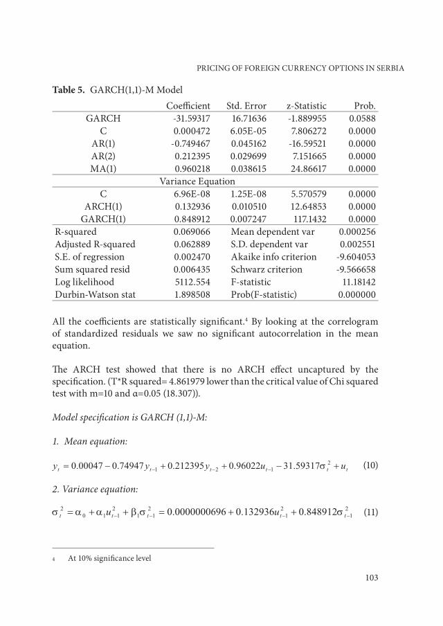
Table 5. GARCH(1,1)-M ModelCoefficient Std. Error z-Statistic Prob.

GARCH -31.59317 16.71636 -1.889955 0.0588C 0.000472 6.05E-05 7.806272 0.0000

AR(1) -0.749467 0.045162 -16.59521 0.0000AR(2) 0.212395 0.029699 7.151665 0.0000MA(1) 0.960218 0.038615 24.86617 0.0000

Variance EquationC 6.96E-08 1.25E-08 5.570579 0.0000

ARCH(1) 0.132936 0.010510 12.64853 0.0000GARCH(1) 0.848912 0.007247 117.1432 0.0000

R-squared 0.069066 Mean dependent var 0.000256Adjusted R-squared 0.062889 S.D. dependent var 0.002551S.E. of regression 0.002470 Akaike info criterion -9.604053Sum squared resid 0.006435 Schwarz criterion -9.566658Log likelihood 5112.554 F-statistic 11.18142Durbin-Watson stat 1.898508 Prob(F-statistic) 0.000000

All the coefficients are statistically significant.4 By looking at the correlogram of standardized residuals we saw no significant autocorrelation in the mean equation.

The ARCH test showed that there is no ARCH effect uncaptured by the specification. (T*R squared= 4.861979 lower than the critical value of Chi squared test with m=10 and α=0.05 (18.307)).

Model specification is GARCH (1,1)-M:

1. Mean equation:

(10)

2. Variance equation:

(11)

4 At 10% significance level

104

Irena Janković

Figure 5. The Conditional Variance

The conditional variance is changing, but the unconditional (long-run) variance of ut is constant and given by expression:

, so long as <1 (12)

The unconditional variance for daily data in our analysis is equal to:

(13)

The unconditional variance is close to S.E. of regression5 squared that is equal to (0.00247)2=0.000006. Standard deviation is equal to the square root of the variance, i.e. = 0.1958134%. This measure is calculated on the daily data basis. In order to get variance and standard deviation on the annual basis we have used the Drost-Nijman formula6 because the simple scaling by the rule σ cannot be implemented in the case of GARCH processes and in any case where we do not have asset returns that are independently and identically distributed (iid). By implementing the Drost-Nijman formula we got an annual variance of7:

5 See Table 5.6 Please refer to Appendix A and Appendix B7 Calculations are provided in Appendix B


105

Var(252)=0.000966240635, and standard deviation of:

σ(252)=3.1084411441% (14)

We implemented exactly this measure of volatility in the Black-Scholes option pricing formula in order to get the prices of the FX options.

We performed the Wald test to check if we had an IGARCH effect in the model. By looking at the p values (F-statistic=8.779302, p=0.0031; Chi-square=8.779302, p=0.003) we rejected the null hypothesis, with the significance level of 5%, that there was an IGARCH effect, meaning that we do not have non-stationarity in volatility. That means that we can use our GARCH model for forecasting and plug the resulting volatility measure into the Black and Scholes formula.

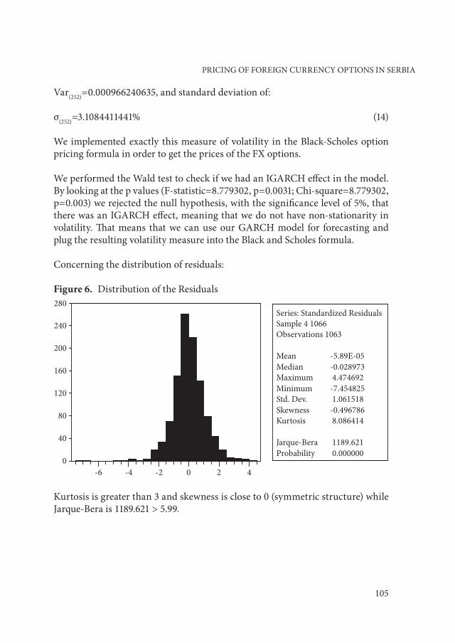
Concerning the distribution of residuals:

Figure 6. Distribution of the Residuals

Kurtosis is greater than 3 and skewness is close to 0 (symmetric structure) while Jarque-Bera is 1189.621 > 5.99.

106

Irena Janković

6. Pricing of FX Options in the Local Market

As the previous analysis shows, the RSD/EUR exchange rate series could be modeled through the ARIMA (2,1,1) specification. Volatility characteristics meet the GARCH (1,1)-M specification. In-the-sample forecast shows good characteristics, meaning that historic volatility is explained well by the model. In this way resulting volatility specification could be used in financial instrument pricing, e.g. plain vanilla options, once they appear on the local exchange. These instruments could then be included in different hedging strategies.

The resulting marginal volatility measure from the model for the RSD/EUR average nominal exchange rate returns can be further plugged into the accommodated Black and Scholes specification8 in order to get prices of the basic FX European options.

C0 = S0e-rfT N(d1) – Xe-rT N(d2) (15)

P0 = Xe-rT N(-d2) - S0e-rfT N(-d1) (16)

,

Let us assume the real situation of buying a 3-month FX European call option contract on RSD/EUR on 20 March 2007. Available input data are:

S0 – current exchange rate=80.7183 (from the National Bank of Serbia)X – exercise price=79.5000r – domestic risk-free interest rate=8.36% (3-month local Government bills’ rate in period under estimation)9

8 See Hull, J. C. (2000) 9 The author is aware that the way the rate of Government bills has been determined in the

Republic of Serbia to date, is not very representative of the risk free rate on the local market. Before improvement in the process of issuing and trading Government bills, it may be a good idea to use the Repo rate as the representative of the risk free rate on the local market instead, although it is not the best solution. If we implement that reference rate for the period in question of 11.4 % p.a. (Source: NBS- Statistics) instead of the Government bill rate, the call option’s value would be 2.690884584, and the put option value would be 0.377803483.


107

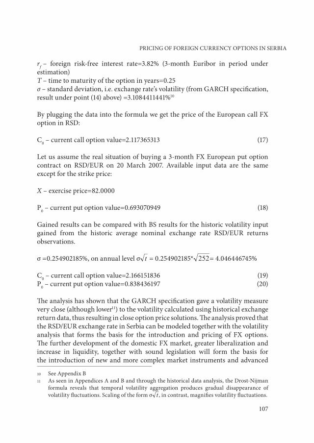
rf – foreign risk-free interest rate=3.82% (3-month Euribor in period under estimation)T – time to maturity of the option in years=0.25σ – standard deviation, i.e. exchange rate’s volatility (from GARCH specification, result under point (14) above) =3.1084411441%10

By plugging the data into the formula we get the price of the European call FX option in RSD:

C0 – current call option value=2.117365313 (17)

Let us assume the real situation of buying a 3-month FX European put option contract on RSD/EUR on 20 March 2007. Available input data are the same except for the strike price:

X – exercise price=82.0000

P0 – current put option value=0.693070949 (18)

Gained results can be compared with BS results for the historic volatility input gained from the historic average nominal exchange rate RSD/EUR returns observations.

σ =0.254902185%, on annual level σ = 0.254902185* = 4.046446745%

C0 – current call option value=2.166151836 (19)P0 – current put option value=0.838436197 (20)

The analysis has shown that the GARCH specification gave a volatility measure very close (although lower11) to the volatility calculated using historical exchange return data, thus resulting in close option price solutions. The analysis proved that the RSD/EUR exchange rate in Serbia can be modeled together with the volatility analysis that forms the basis for the introduction and pricing of FX options. The further development of the domestic FX market, greater liberalization and increase in liquidity, together with sound legislation will form the basis for the introduction of new and more complex market instruments and advanced

10 See Appendix B11 As seen in Appendices A and B and through the historical data analysis, the Drost-Nijman

formula reveals that temporal volatility aggregation produces gradual disappearance of volatility fluctuations. Scaling of the form σ , in contrast, magnifies volatility fluctuations.

108

Irena Janković

pricing techniques. In the initial phase the already present implementation of forward contracts and swap arrangements is appropriate, until the volume of trading reaches the level that would require standardization of contracts and their variety.

7. FX derivatives in Serbia

The FX risk management practice in Serbia is still underdeveloped. However domestic companies and financial institutions are becoming more interested in this topic because they see the adverse effect on their financial results of exchange rate movements and currency exposures on their balance sheets. Institutions connected to foreign markets, either through business activities or through major foreign ownership, are more willing and able to use foreign currency and other derivative contracts. That is the case with most banks in dominant foreign ownership operating in the local market.

In keeping with the goals of risk management, hedging activities focus on the use of interest rate swaps and floors, cross-currency (FX) swaps, swaptions, caps, floors and other types of OTC options. Interest rate swaps are used by banks to turn fixed-income flows into variable-income flows or to convert those issues that are not money market-linked into issues that are, depending on the asset liability structure in their balance sheets. Floors are used to secure a minimum interest rate on money market-linked loans in case of declining market interest rates. In dealing with foreign exchange exposure, in order to hedge anticipated foreign currency interest income against currency risk, they use spot transactions, forward contracts, FX swaps and currency swaps. FX swap is a transaction which involves the actual exchange of two currencies (principal amount only) on a specific date at a rate agreed at the time of conclusion of the contract, and a reverse exchange of the same two currencies at a date further in the future and at a rate agreed at the time of the contract. Currency swap is a contract that commits two counterparties to exchange streams of interest payments in different currencies for an agreed period of time and to exchange principal amounts in different currencies at a pre-agreed exchange rate at maturity.

These are all OTC contracts based on individual needs and agreements between contracting parties. Future development of the local market will lead to standardization and introduction of exchange traded contracts. That opens the door for further education in this area together with the introduction of new instruments in the local FX market.


109

Asteriou, D. and S. G. Hall (2007), Applied Econometrics, Palgrave Macmillan

Black, F. and M. Scholes (1973), “The Pricing of Options and Corporate Liabilities”, Journal of Political Economy, Volume 81, No. 3, pp. 637-654

Bollerslev, T. (1986), “Generalized Autoregressive Conditional Heteroskedasticity”, Journal of Econometrics, Volume 31, pp. 307-327

Brooks, C. (2002), Introductory Econometrics for Finance, Cambridge University Press, Cambridge

Christoffersen, P. and K Jacobs (2004), “Which Volatility for Option Valuation?”, Management Science, Volume 50, pp. 1204-1221

Diebold, F.X. at all. (1998), “Converting 1-day Volatility to h-day Volatility: Scaling by is Worse than You Think”, Wharton Financial Institutions Center, Working Paper 97-34

REFERENCES

8. Conclusion

The Serbian FX market has faced radical changes during its recent development. The FX rates analysis showed that locally formed FX rates can be modeled in the domestic market. The gained econometric model was used in volatility analysis. The resulting GARCH specification volatility measure was implemented as an input in the pricing of theoretically formed currency options in the local market. Analysis showed that there are bases for the pricing of currency options. Implementation of the standardized instruments is expected to follow the further development of the domestic FX market, its size, liquidity and legislative framework. In the beginning the further implementation of forward and swap contracts is appropriate, until the volume of trading reaches levels that would require standardization of contracts and their variety. More complex pricing schemes would then be available and adequate FX management schemes created. This opens space for further research.

FX management is not highly developed in Serbia. However an increase in interest in the topic in recent months has created a demand for further education in this area, which will certainly improve the practical implementation of successful solutions in the local financial market.

110

Irena Janković

Drost, F. C. and T. E. Nijman (1993), “Temporal Aggregation of GARCH Processes”, Econometrica, 61, 909-927

Duan, J. C. (1995), “The GARCH Option Pricing Model”, Mathematical Finance, Volume 5, Issue 1, pp. 13-32

Duan, J. C. (1996), “A Unified Theory of Option Pricing under Stochastic Volatility - from GARCH to Diffusion”, http://www.rotman.utoronto.ca/~jcduan/

Duan, J. C. and J. Wei (1999), “Pricing Foreign Currency and Cross-Currency Options under GARCH”, The Journal of Derivatives, Volume 7, No. 1, pp. 51-63

Ekonomist Media Group (2005, 2006), “Top 300”, www.ekonomist.co.yu

Engle, R. F. (1982), “Autoregressive Conditional Heteroscedasticity with Estimates of Variance of United Kingdom Inflation”, Econometrica, Volume 50, No. 4, pp. 987-1007

Engle, R. F., D. Lilien and R. Robins (1987), “Estimating Time Varying Risk Premia in the Term Structure: The Arch-M Model”, Econometrica, Volume 55, No. 2, pp. 391-407

Hardle, W. and M. Hafner (2000), “Discrete Time Option Pricing with Flexible Volatility Estimation”, Finance and Stochastics, Volume 4, No. 2, pp.189-207

Heston, S. L. and S. Nandi (2000), “A Closed-form GARCH Option Valuation Model”, The Review of Financial Studies, Volume 13, pp. 585-625

Hsieh, K. C. and P. Ritchken (2005), “An Empirical Comparison of GARCH Option Pricing Models”, Review of Derivatives Research, Volume 8, No. 3, pp. 129-150

Hull, J. C. (2000), Options, Futures and Other Derivatives, Prentice Hall

Hull, J. and A. White (1987), “The Pricing of Options on Assets with Stochastic Volatilities”, The Journal of Finance, Volume 42, No. 2, pp. 281-300

Jankovic, I. (2007), Currencies and their Exchanges: Hedging and Investment Applications, Master of Science Thesis, Faculty of Economics, Belgrade

Merton, R. C. (1973), “Theory of Rational Option Pricing”, The Bell Journal of Economics and Management Science, Volume 4, No. 1, Spring, pp. 141-183

Nelson, D. (1990), “ARCH Models as Diffusion Approximations”, Journal of Econometrics, Volume 45, pp. 7-38

Noh, J., R. Engle and A. Kane (1994), “Forecasting Volatility and Option Prices of the S&P 500 Index”, Journal of Derivatives, Volume 2, pp. 17-30

Tsay, R. S. (2005), Analysis of Financial Time Series, 2nd Edition, Wiley


111

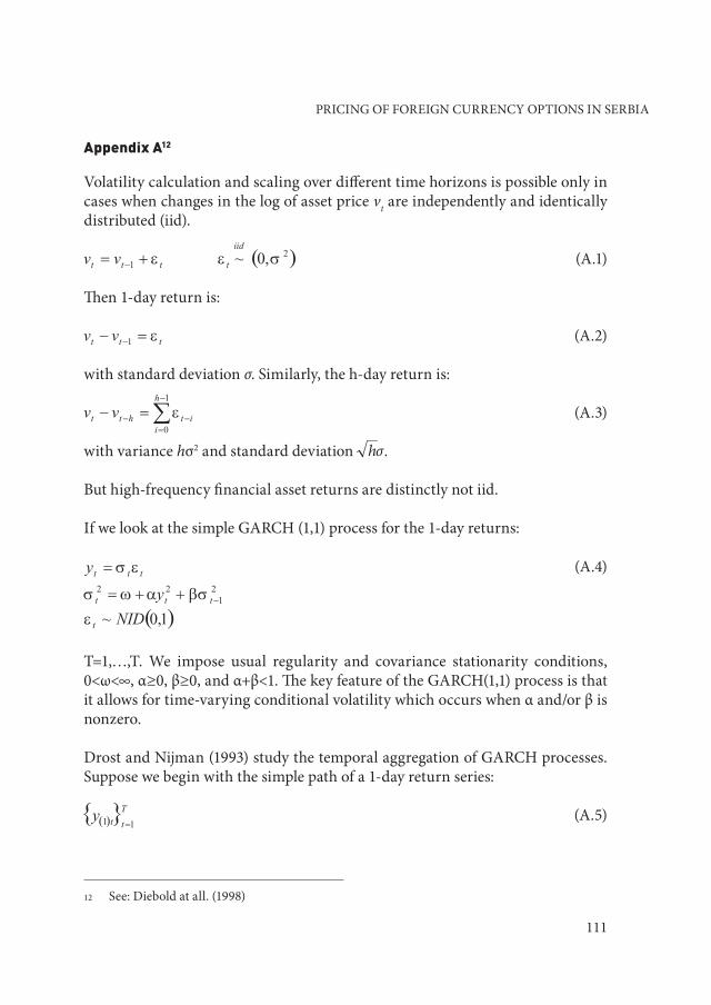
Appendix A12

Volatility calculation and scaling over different time horizons is possible only in cases when changes in the log of asset price vt are independently and identically distributed (iid).

(A.1)

Then 1-day return is:

(A.2)

with standard deviation σ. Similarly, the h-day return is:

(A.3)

with variance hσ2 and standard deviation .

But high-frequency financial asset returns are distinctly not iid.

If we look at the simple GARCH (1,1) process for the 1-day returns:

(A.4)

T=1,…,T. We impose usual regularity and covariance stationarity conditions, 0<ω<∞, α≥0, β≥0, and α+β<1. The key feature of the GARCH(1,1) process is that it allows for time-varying conditional volatility which occurs when α and/or β is nonzero.

Drost and Nijman (1993) study the temporal aggregation of GARCH processes. Suppose we begin with the simple path of a 1-day return series:

(A.5)

12 See: Diebold at all. (1998)

112

Irena Janković

which follows the GARCH(1,1) process above. They show that under regularity conditions, the corresponding sample path of h-day returns:

(A.6)

similarly, follows a GARCH(1,1) process with:

(A.7)

where

(A.8)

and |β(h)| < 1 is the solution of the quadratic equation

(A.9)

where

(A.10)

and k is the kurtosis of yt.

The Drost-Nijman formula is important because it is the key to correct conversion of 1-day volatility to h-day volatility. The simple scaling formula is not an accurate approximation to the Drost-Nijman formula. As h→∞, analysis of the Drost-Nijman formula reveals that α(h)→0 and β(h)→0 which is to say that temporal aggregation produces gradual disappearance of volatility fluctuations. Scaling, in contrast, magnifies volatility fluctuations.


113

Appendix B

Through implementation of the presented Drost-Nijman formula in Appendix A we are finding the annual volatility for our GARCH specification under (11) rewritten here:

(B.1)

The Drost-Nijman formula is as follows:

(B.2)

where

(B.3)

and |β1(252)|<1 is the solution of the quadratic equation

(B.4)

where

(B.5)

By inserting the values for α0=0.0000000696, α1=0.132936, β1=0.848912 from (B.1) and value for k=8.086414 from Figure 6. into the specifications under (B.3), (B.4) and (B.5) we got the following results:

(B.6)

114

Irena Janković

(B.7)

(B.8)

By solving the quadratic equation:

We found |β1(252)|<1 as the solution:

(B.9)

And:

(B.10)

We used the gained results under (B.6), (B.9) and (B.10) in the formula for the unconditional (long-run) annual variance and standard deviation and got the following results:


115

(B.11)

The result for annual volatility is further implemented as input in the Black-Scholes formula.

pricing of foreign currency options in the serbian … · pricing of foreign currency options in...

Documents