Pricing Schemes in Electric Energy Markets

by

Chao Li

A Thesis Presented in Partial Fulfillmentof the Requirements for the Degree

Master of Science

Approved April 2016 by theGraduate Supervisory Committee:

Kory W. Hedman, ChairLalitha SankarAnna Scaglione

ARIZONA STATE UNIVERSITY

May 2016

ABSTRACT

Two thirds of the U.S. power systems are operated under market structures. A good

market design should maximize social welfare and give market participants proper

incentives to follow market solutions. Pricing schemes play very important roles in

market design.

Locational marginal pricing scheme is the core pricing scheme in energy markets.

Locational marginal prices are good pricing signals for dispatch marginal costs. How-

ever, the locational marginal prices alone are not incentive compatible since energy

markets are non-convex markets. Locational marginal prices capture dispatch costs

but fail to capture commitment costs such as startup cost, no-load cost, and shut-

down cost. As a result, uplift payments are paid to generators in markets in order

to provide incentives for generators to follow market solutions. The uplift payments

distort pricing signals.

In this thesis, pricing schemes in electric energy markets are studied. In the first

part, convex hull pricing scheme is studied and the pricing model is extended with

network constraints. The subgradient algorithm is applied to solve the pricing model.

In the second part, a stochastic dispatchable pricing model is proposed to better

address the non-convexity and uncertainty issues in day-ahead energy markets. In

the third part, an energy storage arbitrage model with the current locational marginal

price scheme is studied. Numerical test cases are studied to show the arguments in

this thesis.

The overall market and pricing scheme design is a very complex problem. This

thesis gives a thorough overview of pricing schemes in day-ahead energy markets and

addressed several key issues in the markets. New pricing schemes are proposed to

improve market efficiency.

i

ACKNOWLEDGMENTS

I would like to thank my thesis chair, Dr. Kory Hedman, for his guidance and

support to finish this thesis. Dr. Hedman is an expert in energy markets and talented

in teaching. Most of my knowledge on energy markets is learned from his EEE 598

Energy Markets class or the individual meeting with him. He has been very supportive

for my research: helping me publish papers and writing me recommendation letters

for my internship and awards applications. Thank you very much.

I would like to thank Dr. Anna Scaglione and Dr. Lalitha Sankar for being on

my thesis committee. I would like to thank Dr. Audun Botterud and Dr. John Birge

for the help on stochastic dispatchable pricing scheme.

I would like to thank Power Systems Engineering Research Center (PSERC) to

provide funding to support my study.

I would like thank all who has provided help during my study and research. I am

very grateful.

ii

TABLE OF CONTENTS

Page

LIST OF TABLES . . . . . . . . . . . . . . . . . . . . . . . . . . . . . . . . . . . . . . . . . . . . . . . . . . . . . . . . . v

LIST OF FIGURES . . . . . . . . . . . . . . . . . . . . . . . . . . . . . . . . . . . . . . . . . . . . . . . . . . . . . . . . vi

CHAPTER

1 INTRODUCTION . . . . . . . . . . . . . . . . . . . . . . . . . . . . . . . . . . . . . . . . . . . . . . . . . . . 1

1.1 Background . . . . . . . . . . . . . . . . . . . . . . . . . . . . . . . . . . . . . . . . . . . . . . . . . . . . 1

1.2 Research Focus . . . . . . . . . . . . . . . . . . . . . . . . . . . . . . . . . . . . . . . . . . . . . . . . . 5

1.3 Summary of Chapters . . . . . . . . . . . . . . . . . . . . . . . . . . . . . . . . . . . . . . . . . . . 6

2 CONVEX HULL PRICING . . . . . . . . . . . . . . . . . . . . . . . . . . . . . . . . . . . . . . . . . . 8

2.1 Introduction . . . . . . . . . . . . . . . . . . . . . . . . . . . . . . . . . . . . . . . . . . . . . . . . . . . . 8

2.2 Convex Hull Pricing . . . . . . . . . . . . . . . . . . . . . . . . . . . . . . . . . . . . . . . . . . . . 10

2.3 Formulation . . . . . . . . . . . . . . . . . . . . . . . . . . . . . . . . . . . . . . . . . . . . . . . . . . . . 13

2.3.1 Economic Dispatch Unit Commitment . . . . . . . . . . . . . . . . . . . . . 13

2.3.2 Direct Current Optimal Power Flow Unit Commitment . . . . . 14

2.4 Methods . . . . . . . . . . . . . . . . . . . . . . . . . . . . . . . . . . . . . . . . . . . . . . . . . . . . . . . 14

2.4.1 LMP Calculation . . . . . . . . . . . . . . . . . . . . . . . . . . . . . . . . . . . . . . . . 14

2.4.2 CHP Calculation. . . . . . . . . . . . . . . . . . . . . . . . . . . . . . . . . . . . . . . . . 15

2.4.3 Subgradient Algorithm . . . . . . . . . . . . . . . . . . . . . . . . . . . . . . . . . . . 18

2.5 Test Results . . . . . . . . . . . . . . . . . . . . . . . . . . . . . . . . . . . . . . . . . . . . . . . . . . . . 19

2.6 Conclusions . . . . . . . . . . . . . . . . . . . . . . . . . . . . . . . . . . . . . . . . . . . . . . . . . . . . 24

3 STOCHASTIC DISPATCHABLE PRICING . . . . . . . . . . . . . . . . . . . . . . . . . . 26

3.1 Introduction . . . . . . . . . . . . . . . . . . . . . . . . . . . . . . . . . . . . . . . . . . . . . . . . . . . . 26

3.2 Pricing Model . . . . . . . . . . . . . . . . . . . . . . . . . . . . . . . . . . . . . . . . . . . . . . . . . . 30

3.2.1 Model Overview . . . . . . . . . . . . . . . . . . . . . . . . . . . . . . . . . . . . . . . . . 31

3.2.2 Stochastic Pricing Framework . . . . . . . . . . . . . . . . . . . . . . . . . . . . . 32

iii

CHAPTER Page

3.2.3 Dispatchable Relaxation . . . . . . . . . . . . . . . . . . . . . . . . . . . . . . . . . . 34

3.2.4 DAM and RTM Process . . . . . . . . . . . . . . . . . . . . . . . . . . . . . . . . . . 36

3.3 Test Cases . . . . . . . . . . . . . . . . . . . . . . . . . . . . . . . . . . . . . . . . . . . . . . . . . . . . . 38

3.3.1 6-Bus System . . . . . . . . . . . . . . . . . . . . . . . . . . . . . . . . . . . . . . . . . . . . 39

3.3.2 IEEE 118-Bus System . . . . . . . . . . . . . . . . . . . . . . . . . . . . . . . . . . . . 43

3.4 Conclusions . . . . . . . . . . . . . . . . . . . . . . . . . . . . . . . . . . . . . . . . . . . . . . . . . . . . 47

4 ARBITRAGE IN ENERGY MARKETS . . . . . . . . . . . . . . . . . . . . . . . . . . . . . . 49

4.1 Introduction . . . . . . . . . . . . . . . . . . . . . . . . . . . . . . . . . . . . . . . . . . . . . . . . . . . . 49

4.2 Mathematical Formulations . . . . . . . . . . . . . . . . . . . . . . . . . . . . . . . . . . . . . . 52

4.2.1 Location Selection Model . . . . . . . . . . . . . . . . . . . . . . . . . . . . . . . . . 52

4.2.2 SCUC and SCED . . . . . . . . . . . . . . . . . . . . . . . . . . . . . . . . . . . . . . . . 54

4.2.3 Arbitrage Model . . . . . . . . . . . . . . . . . . . . . . . . . . . . . . . . . . . . . . . . . 57

4.3 Electric Energy Storage Charging Policies . . . . . . . . . . . . . . . . . . . . . . . . 63

4.3.1 Forecasting-belief Policy . . . . . . . . . . . . . . . . . . . . . . . . . . . . . . . . . . 63

4.3.2 Robust Policy . . . . . . . . . . . . . . . . . . . . . . . . . . . . . . . . . . . . . . . . . . . 64

4.3.3 Dynamic Policy . . . . . . . . . . . . . . . . . . . . . . . . . . . . . . . . . . . . . . . . . . 64

4.4 Case Study and Computational Results . . . . . . . . . . . . . . . . . . . . . . . . . . 65

4.5 Conclusions . . . . . . . . . . . . . . . . . . . . . . . . . . . . . . . . . . . . . . . . . . . . . . . . . . . . 70

5 CONCLUSIONS AND FUTURE WORK . . . . . . . . . . . . . . . . . . . . . . . . . . . . . 72

5.1 Conclusions . . . . . . . . . . . . . . . . . . . . . . . . . . . . . . . . . . . . . . . . . . . . . . . . . . . . 72

5.2 Future Work . . . . . . . . . . . . . . . . . . . . . . . . . . . . . . . . . . . . . . . . . . . . . . . . . . . 76

REFERENCES . . . . . . . . . . . . . . . . . . . . . . . . . . . . . . . . . . . . . . . . . . . . . . . . . . . . . . . . . . . . 78

APPENDIX

A NOMENCLATURE . . . . . . . . . . . . . . . . . . . . . . . . . . . . . . . . . . . . . . . . . . . . . . . . . 82

iv

LIST OF TABLES

Table Page

2.1 Generator Bids . . . . . . . . . . . . . . . . . . . . . . . . . . . . . . . . . . . . . . . . . . . . . . . . . . . . 11

2.2 Uplift Payment Comparison . . . . . . . . . . . . . . . . . . . . . . . . . . . . . . . . . . . . . . . . 19

2.3 Load Payment and Generation Rent Comparison under ED UC . . . . . . . 20

2.4 Load Payment and Generation Rent Comparison under DCOPF UC . . . 20

3.1 6-Bus System Generator Basic Data . . . . . . . . . . . . . . . . . . . . . . . . . . . . . . . . . 40

3.2 6-Bus System Generator Cost Data . . . . . . . . . . . . . . . . . . . . . . . . . . . . . . . . . 40

3.3 Market Allocation Comparison . . . . . . . . . . . . . . . . . . . . . . . . . . . . . . . . . . . . . . 41

3.4 Generator and Wind Farm Profit Comparison . . . . . . . . . . . . . . . . . . . . . . . . 41

3.5 Market Allocation Comparison for High-load Day . . . . . . . . . . . . . . . . . . . . 43

3.6 Selected Generator Data . . . . . . . . . . . . . . . . . . . . . . . . . . . . . . . . . . . . . . . . . . . . 43

3.7 Generator and Wind Farm Profit Comparison for High-load Day . . . . . . 44

3.8 Market Allocation under Different Load Profiles . . . . . . . . . . . . . . . . . . . . . . 45

3.9 Generator and Wind Farm Profit Comparison . . . . . . . . . . . . . . . . . . . . . . . . 46

3.10 LMP Differences between DAM and RTM Comparison . . . . . . . . . . . . . . . 46

4.1 LMP Comparison under 100MW Power Capacity . . . . . . . . . . . . . . . . . . . . . 66

4.2 LMP Comparison under 150MW Power Capacity . . . . . . . . . . . . . . . . . . . . . 67

4.3 Arbitrage Comparison under Different Locations . . . . . . . . . . . . . . . . . . . . . 68

4.4 Arbitrage Comparison under Different Load Profiles . . . . . . . . . . . . . . . . . . 69

4.5 Arbitrage Comparison under Different EES Efficiency . . . . . . . . . . . . . . . . 69

4.6 Arbitrage Comparison under Different Policies . . . . . . . . . . . . . . . . . . . . . . . 70

v

LIST OF FIGURES

Figure Page

1.1 Structure of Electric Power Systems . . . . . . . . . . . . . . . . . . . . . . . . . . . . . . . . . 1

1.2 RTO/ISOs in the U.S. . . . . . . . . . . . . . . . . . . . . . . . . . . . . . . . . . . . . . . . . . . . . . . 2

1.3 DAM Process in MISO . . . . . . . . . . . . . . . . . . . . . . . . . . . . . . . . . . . . . . . . . . . . . 4

2.1 Total Cost with respect to Total Loads . . . . . . . . . . . . . . . . . . . . . . . . . . . . . . 12

2.2 Marginal Cost with respect to Total Loads . . . . . . . . . . . . . . . . . . . . . . . . . . . 12

2.3 Prices Comparison by Period under ED UC . . . . . . . . . . . . . . . . . . . . . . . . . . 21

2.4 Prices Comparison for Period 6 under DCOPF UC . . . . . . . . . . . . . . . . . . . 22

2.5 Prices Comparison for Period 9 under DCOPF UC . . . . . . . . . . . . . . . . . . . 23

2.6 Prices Comparison for Period 20 under DCOPF UC . . . . . . . . . . . . . . . . . . 23

2.7 Prices Comparison with respect to Total Load Percentage . . . . . . . . . . . . . 24

3.1 DAM Clearing Process under Proposed Pricing Scheme . . . . . . . . . . . . . . . 37

3.2 LMP with respect to Total Load at Bus 6 in Period 14 . . . . . . . . . . . . . . . 42

3.3 Prices with respect to Total Load in Period 14 . . . . . . . . . . . . . . . . . . . . . . . 42

3.4 LMP Comparison across Periods at Bus 100 . . . . . . . . . . . . . . . . . . . . . . . . . 44

3.5 LMPs Comparison across Periods at Bus 113 . . . . . . . . . . . . . . . . . . . . . . . . 45

4.1 DAM Structure . . . . . . . . . . . . . . . . . . . . . . . . . . . . . . . . . . . . . . . . . . . . . . . . . . . . 54

4.2 EES Charging/Discharging Decision Procedure . . . . . . . . . . . . . . . . . . . . . . . 63

4.3 Dynamic Policy Procedure . . . . . . . . . . . . . . . . . . . . . . . . . . . . . . . . . . . . . . . . . . 65

vi

Chapter 1

INTRODUCTION

1.1 Background

The electric power grid is one of the most complex engineered machines ever cre-

ated. The National Academy of Engineering ranks the electrification as the greatest

achievement of the 20th century (National Academy of Engineering, 2015). Electric

power systems can be divided into four sub-systems: the generation, transmission,

distribution, and load systems, as illustrated in Figure 1.1 (U.S.-Canada Power Sys-

tem, 2004).

Figure 1.1: Structure of Electric Power Systems

(U.S.-Canada Power System, 2004)

Followed the Federal Energy Policy Act in 1992, the concepts of regional trans-

mission organization (RTO) and independent system operator (ISO) were first intro-

1

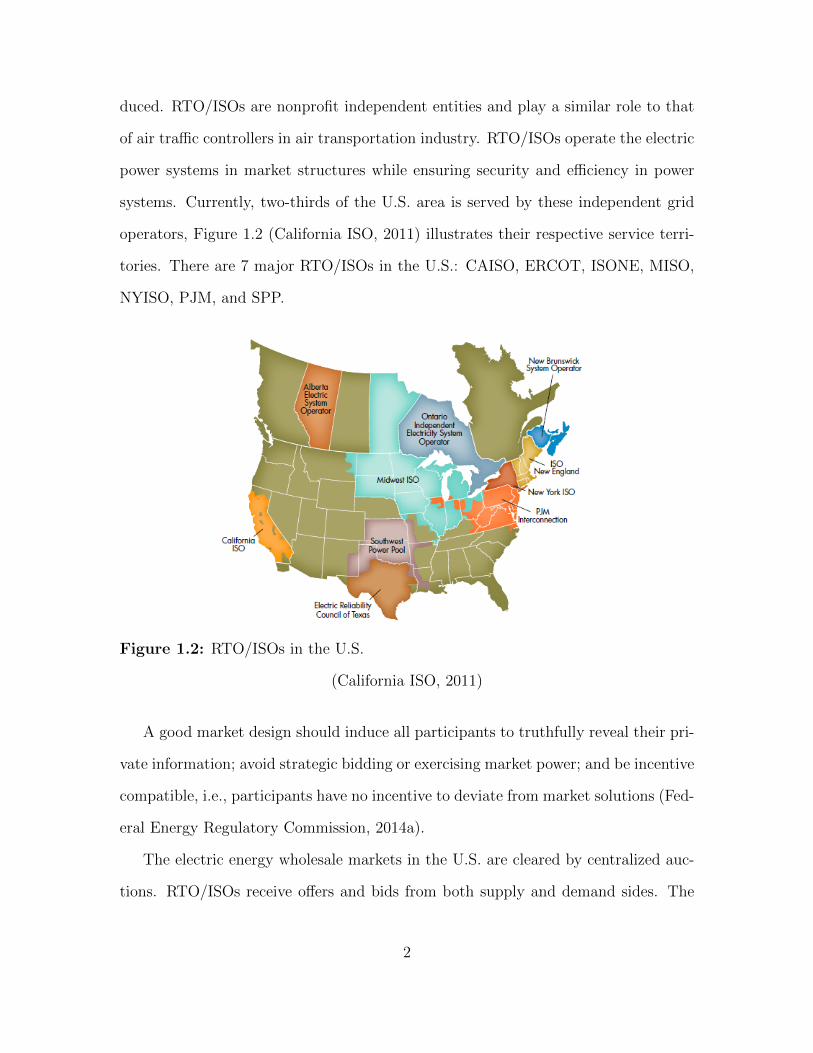
duced. RTO/ISOs are nonprofit independent entities and play a similar role to that

of air traffic controllers in air transportation industry. RTO/ISOs operate the electric

power systems in market structures while ensuring security and efficiency in power

systems. Currently, two-thirds of the U.S. area is served by these independent grid

operators, Figure 1.2 (California ISO, 2011) illustrates their respective service terri-

tories. There are 7 major RTO/ISOs in the U.S.: CAISO, ERCOT, ISONE, MISO,

NYISO, PJM, and SPP.

Figure 1.2: RTO/ISOs in the U.S.

(California ISO, 2011)

A good market design should induce all participants to truthfully reveal their pri-

vate information; avoid strategic bidding or exercising market power; and be incentive

compatible, i.e., participants have no incentive to deviate from market solutions (Fed-

eral Energy Regulatory Commission, 2014a).

The electric energy wholesale markets in the U.S. are cleared by centralized auc-

tions. RTO/ISOs receive offers and bids from both supply and demand sides. The

2

bidders from supply side are mainly generators and the bidders from demand side

are mainly load serving entities (LSE). The offers and bids include mainly prices and

capacities that the market participants would like to supply or consume. RTO/ISOs

clear the energy markets by running market models based on the collected bids as

model inputs.

The energy markets are multi-settlement markets including mainly day-ahead

market (DAM) and real-time market (RTM). The DAM and RTM represent a for-

ward market and a spot market. The forward (financial) market is in advance of the

corresponding real-time spot (physical) market where agreements are made based on

the future delivery at agreed upon forward contracts. Although different RTO/ISOs

have different market clearing processes and terminologies for the processes, there is

a general market clearing process describes as follows. In DAM, RTO/ISOs: a) col-

lect bids, b) run security-constrained unit commitment (SCUC) model to determine

generator commitments, c) fix commitments, run security-constrained economic dis-

patch (SCED) model to determine dispatch solution, d) post DAM solution and DAM

prices. In RTM, RTO/ISOs: a) run SCED to balance energy supply and demand,

b) determine RTM prices. Figure 1.3 (Midcontinent ISO, 2007) illustrate the DAM

process in MISO.

Pricing schemes are important for market designs since market participants will

make operating and investment decisions based on pricing signals (Hogan, 2014). A

pricing signal is the informational value of the market clearing prices that are used

to settle the markets (O’Neill, 2009). ISONE proposed three principles to evaluate

pricing signals: efficiency, transparency, and simplicity (ISO New England, 2014).

Efficiency evaluates whether the offered prices can maximize social welfare and all

participants would like to follow market solutions. Transparency evaluates whether

much is known by many, i.e., every participant knows the prices other receive. Sim-

3

Figure 1.3: DAM Process in MISO

(Midcontinent ISO, 2007)

plicity evaluates whether the pricing scheme is simple and easy to be interpreted.

In the energy markets in the U.S., a uniform pricing scheme is adopted. The

uniform pricing clears the market at the marginal unit’s cost and all selected bids

are paid at a uniform market clearing price. Starting form late 90s, RTO/ISOs

began to switch from zonal pricing to nodal pricing for generators (Pope, 2014).

Locational marginal price (LMP) is the core of pricing in all RTO/ISOs’ energy

markets nowadays. The LMP scheme is a uniform pricing mechanism and emphasizes

the locational differences caused by the limits and losses in transmission.

Power flow problems are non-linear, non-convex problems (Wood and Wollenberg,

1996). RTO/ISOs adopt linearized power flow models to approximate the real power

flow in the market models, as known as direct current optimal power flow (DCOPF)

models (Federal Energy Regulatory Commission, 2011). A generalized market model

is represented as follows:

4

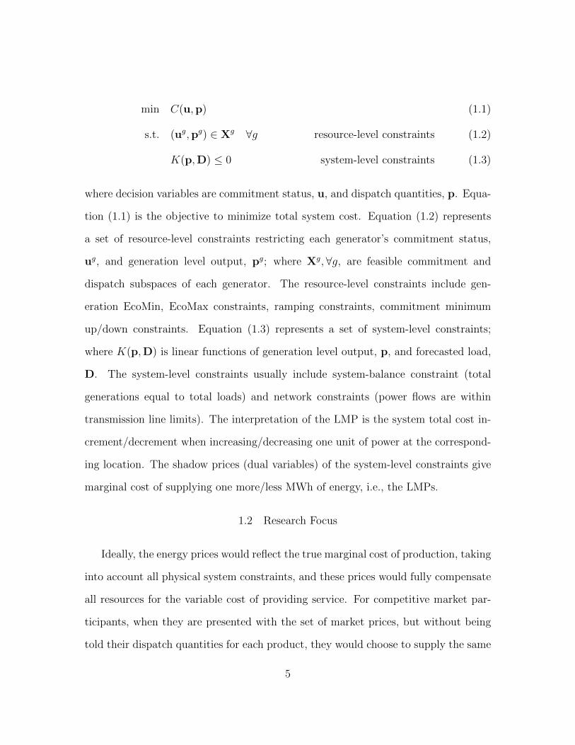
min C(u,p) (1.1)

s.t. (ug,pg) ∈ Xg ∀g resource-level constraints (1.2)

K(p,D) ≤ 0 system-level constraints (1.3)

where decision variables are commitment status, u, and dispatch quantities, p. Equa-

tion (1.1) is the objective to minimize total system cost. Equation (1.2) represents

a set of resource-level constraints restricting each generator’s commitment status,

ug, and generation level output, pg; where Xg,∀g, are feasible commitment and

dispatch subspaces of each generator. The resource-level constraints include gen-

eration EcoMin, EcoMax constraints, ramping constraints, commitment minimum

up/down constraints. Equation (1.3) represents a set of system-level constraints;

where K(p,D) is linear functions of generation level output, p, and forecasted load,

D. The system-level constraints usually include system-balance constraint (total

generations equal to total loads) and network constraints (power flows are within

transmission line limits). The interpretation of the LMP is the system total cost in-

crement/decrement when increasing/decreasing one unit of power at the correspond-

ing location. The shadow prices (dual variables) of the system-level constraints give

marginal cost of supplying one more/less MWh of energy, i.e., the LMPs.

1.2 Research Focus

Ideally, the energy prices would reflect the true marginal cost of production, taking

into account all physical system constraints, and these prices would fully compensate

all resources for the variable cost of providing service. For competitive market par-

ticipants, when they are presented with the set of market prices, but without being

told their dispatch quantities for each product, they would choose to supply the same

5

amount of each product for the dispatch as the market solution in order to maximize

their profits (Federal Energy Regulatory Commission, 2014a).

LMPs are good pricing signals for single-period (short-run) dispatch marginal

costs. However, the LMPs alone are not incentive compatible since energy markets

are non-convex markets. The non-convexities of energy markets are a result of many

reasons. The most important reason is that the commitment status is a binary de-

cision and the EcoMin of most generators are not zero, i.e., most generators are not

perfectly partially dispatchable. Moreover, minimum up/down time requirements re-

strict generators online/offline when they may not provide economic efficiency for the

corresponding period. LMPs capture dispatch costs, but fail to capture commitment

costs such as startup cost, no-load cost, and shutdown cost. In fact, the discrete

nature of commitment decisions, startup costs, and no-load costs may prevent the

existence of a set of incentive compatible market clearing prices in DAM since there

is generally no set of market prices that would induce profit maximizing generators

and loads to voluntarily follow the pricing scheme (Gribik, 2007).

In this thesis, the focus is on studying and improving the current pricing scheme,

i.e., LMP scheme. First, convex hull pricing scheme is studied and extended to

network-constrained model. Second, prices inconsistency between DAM and RTM is

studied, and a stochastic dispatchable pricing scheme is proposed. Third, under the

current energy market structure and pricing scheme, price arbitrage of electric energy

storage is studied and analyzed.

1.3 Summary of Chapters

In Chapter 2, two pricing schemes in energy markets are studied, LMP scheme

and convex hull pricing pricing. The effects of these two pricing mechanisms are

compared with regards to the allocation of the market surplus between generators and

6

loads. The two pricing mechanisms are also analyzed with regards to the required

uplift payments. The results confirm that uplift payments are reduced under the

convex hull pricing mechanism. However, convex hull pricing does not appropriately

represent the marginal market clearing price for the market dispatch solution.

In Chapter 3, a stochastic dispatchable locational marginal pricing scheme is pro-

posed to better represent the non-convexity and uncertainty in DAM markets. The

advantages of the proposed pricing scheme are analyzed and two test cases are pre-

sented to compare different pricing schemes.

In Chapter 4, the impacts of electric energy storage arbitrage in energy markets are

studied. The charging or discharging activities for large-scale storage units may have

huge impacts on real-time LMPs. An optimization model is proposed to maximize

the arbitrager’s profits with the consideration of the charging and discharging impacts

on the LMPs. Three charging policies are discussed to handle the uncertainty that

the intermittent wind penetration brings to the power grid. Finally, an IEEE 118-bus

system case study is carried out to evaluate the model and the different charging

policies.

Chapter 5 concludes this thesis and discusses potential future research directions.

7

Chapter 2

CONVEX HULL PRICING

2.1 Introduction

The wholesale electricity markets in the U.S. are designed to promote the effi-

cient delivery of electric power between generators and loads. The DAM solution is

determined by solving SCUC and SCED problems to obtain the least-cost solution

to satisfy the load, while ensuring system reliability. The pricing mechanism used

within energy markets should incentivize generators and loads to follow the market

solution.

Due to the non-convex nature of electricity markets, there may not exist a linear

marginal pricing mechanism for electricity that properly incentivizes all market par-

ticipants to follow the market solution (O’Neill et al., 2005). Thus, a multi-component

pricing mechanism is required to properly incentivize all market participants.

As a result, uplift payments are paid to generators in order to provide incentives

for generators to follow market solutions. Uplift payments can be categorized into

two types: make whole payments (MWPs) and lost opportunity costs (LOCs) (ISO

New England, 2015). MWPs are paid when a generator’s revenue is not enough to

cover its costs, including both commitment costs and dispatch costs. MWPs bring a

generator’s profit to zero, make the generator indifferent between following the market

solutions and doing nothing. LOCs are paid when a generator is restricted to lower

down generation level to provide reserves while the generator can make more profits

if it increases the output level, since the market price is higher than the generator’s

marginal cost. Uplift payments distort price signals and hurt the transparency of

8

the pricing. Uplift is a symptom rather than a cause of price formation problems.

The focus should be on improving pricing efficiencies, rather than on reducing uplift

payments (Pope, 2014). The uplift payment may not be eliminated due to the non-

convexity of energy markets.

The current pricing mechanism found in many RTO/ISOs consists of a locational

uniform price based on the LMP to deliver electric power to the location and a

discriminatory uplift payment for commitment. To determine the LMPs, the UC

problem is first solved to obtain the least-cost solution to satisfy the load. The

binary commitment variables are then fixed to their optimal values and the LMPs

are determined by the dual solution of the node-balance constraints. For the UC

problem with fixed commitments, LMP provides incentives for market participants

to follow the market dispatch solution; however, LMP may not properly incentivize

generators to follow the market commitment solution due to the non-convex nature

of electricity markets (Hogan and Ring, 2003; Gribik et al., 2007). Specifically, LMP

is not influenced by the fixed costs associated with commitment, such as startup and

no-load costs. In order to provide proper market incentives for commitment, the

RTO/ISOs provide uplifts to generators if their revenue does not cover their total

costs; these uplifts are decided at the end of every day.

Currently, many RTO/ISOs pay uplift payments only to generators. The associ-

ated costs are then distributed uniformly amongst the load according to the percent

of total load in order to maintain a locational uniform pricing mechanism on the load

side. These uplift payments can raise load payments above their marginal bids, which

can incentivize price sensitive loads to deviate from the market solution.

Convex hull pricing (CHP) scheme (Gribik et al., 2007), sometimes referred as

extended locational marginal pricing (ELMP), is an alternative pricing mechanism,

which is the closest locational uniform price to clearing the market while also mini-

9

mizing the total uplift payments required to properly incentivize market participants

to follow the market solution (Hogan and Ring, 2003).

In this chapter, the effects of the LMP and CHP schemes on the allocation of the

market surplus between suppliers and loads are studied. The work in this chapter is

based on a joint work with Greg Thompson. Greg Thompson did literature review

for the topic and I developed the rest of the work. For each pricing mechanism, the

magnitude of the generation rent and load payment is determined under two different

UC models and varying levels of load. The initial model builds off of the model used

in (Wang et al., 2012) by including generator minimum up/down time and ramp-rate

constraints. The second model extends the first by including transmission constraints

based on the direct current optimal power flow (DCOPF) approximation.

The organization of the chapter is as follows. Section 2.2 introduces the concepts of

CHP. Section 2.3 gives the formulations of the proposed models. Section 2.4 describes

the methods for calculating LMP and CHP. Section 2.5 analyzes the effects of the

pricing mechanisms based on the IEEE RTS96 single zone test case. Conclusions are

presented in section 2.6.

2.2 Convex Hull Pricing

With the issues of current utilized LMP (standard LMP) in non-convex energy

markets, CHP scheme was proposed in Hogan and Ring (2003) and Gribik et al.

(2007). CHP takes the dual of whole unit commitment model, sets prices as the

Lagrangian multipliers of node balance constraints. Since the Lagrangian multipliers

represent the slope of the convex hull of the total cost function, the pricing scheme

is named as CHP scheme. CHP scheme aims at giving better pricing signals.

The Lagrangian dual of UC problem is equivalent to a problem that maximize each

generator’s profit given a set of market clearing prices. Hogan and Ring (2003) proved

10

that CHP scheme minimizes uplift payment. Moreover, CHP gives a monotonically

non-decreasing total cost function with respect to total load demand, in other words,

higher price under higher demand.

The following example, which is modified based on examples in Gribik et al.

(2007), is given to illustrate CHP scheme. Table 2.1 summarizes generators’ bids in

this example.

Table 2.1: Generator BidsGen G1 G2 G3fixed cost ($) 50 300 100EcoMin (MW) 0 10 50EcoMax (MW) 20 100 100variable cost ($/MW) 40 10 20

In this example, there are three generators with different biding parameters. Fig-

ure 2.1 shows the total cost function with respect to total load demand. The blue

curve represents the total cost curve under standard LMP scheme. It can be seen

that this blue line is not a convex function. Moreover, it is not even a continuous

function. The non-convexity is due to the discrete nature of unit commitment as

discussed in the previous section. As load increases, new resource will be committed

which causes the jumps in total cost function. The red curve represents the convex

hull of the total cost function.

Figure 2.2 represents the corresponding energy prices. The price under standard

LMP goes up and down as total loads increase, while the price under CHP is mono-

tonically non-decreasing.

Uplift payment is required in both standard LMP and CHP schemes. Under

standard LMP, for instance, when total load is 50MW, the most economic dispatch

is to commit G2 only and dispatch 50MW. The total cost is 300 + 10 ∗ 50 = 800.

However, the energy is priced at $10/MW, the revenue of the G2 is 10 ∗ 50 = 500.

The received revenue is not enough to cover the total cost. Then, G2 has no incentive

11

Figure 2.1: Total Cost with respect to Total Loads

Figure 2.2: Marginal Cost with respect to Total Loads

to commit and generating power since it loses money. In order to maximize social

welfare, i.e., encourage generator to stick with the most economic dispatch, RTO/ISO

pays G2 $300 to bring its profit from negative to zero. Similarly, under CHP scheme,

when the total load demand is 110MW, the optimal dispatch solution will be that G2

produces 100MW and G1 produces 10MW. The total cost for G1 is 50+10∗40 = 450.

The energy is priced at $21/MW, thus the revenue of G1 is 10 ∗ 21 = 210. An uplift

payment of $240 is required.

12

2.3 Formulation

The UC models presented here are based on Hedman et al. (2010). Subsec-

tion 2.3.1 gives the formulation for the ED UC model while subsection 2.3.2 gives

the DCOPF UC model.

2.3.1 Economic Dispatch Unit Commitment

min∑∀t

∑∀g

(CSUg vgt + CNL

g ugt + Cgpgt)

(2.1)

s.t.∑∀g

pgt =∑∀n

Dnt ∀t (2.2)

Pming ugt ≤ pgt ≤ Pmax

g ugt ∀g, t (2.3)

vgt − wgt = ugt − ug,t−1 ∀g, t (2.4)

t∑i=t−UT g+1

vgi ≤ ugt ∀g, t (2.5)

t∑i=t−DT g+1

wgi ≤ 1− ugt ∀g, t (2.6)

pgt − pg,t−1 ≤ Rhrg ug,t−1 +RSU

g vgt ∀g, t (2.7)

pg,t−1 − pgt ≤ Rhrg ugt +RSD

g wgt ∀g, t (2.8)

0 ≤ vgt, wgt ≤ 1 ∀g, t (2.9)

ugt ∈ {0, 1} ∀g, t (2.10)

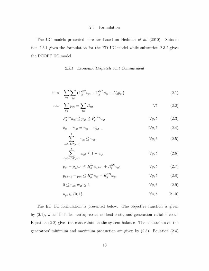
The ED UC formulation is presented below. The objective function is given

by (2.1), which includes startup costs, no-load costs, and generation variable costs.

Equation (2.2) gives the constraints on the system balance. The constraints on the

generators’ minimum and maximum production are given by (2.3). Equation (2.4)

13

specifies the relations between the UC status variables and startup, shutdown vari-

ables. Equations (2.5) and (2.6) give the constraints on the generators’ minimum

up/down time, which are facet defining constraints for the u, v restriction (Rajan and

Takriti, 2005). Generator ramp-rate constraints are given by (2.7) and (2.8). Equa-

tion (2.9) define the bounds on startup and shutdown variables. Equation (2.10)

defines the UC status variables as binary. Note that (2.9)-(2.10), along with (2.4)-

(2.6), force the startup and shutdown variables to be binary even though they are

relaxed to be continuous.

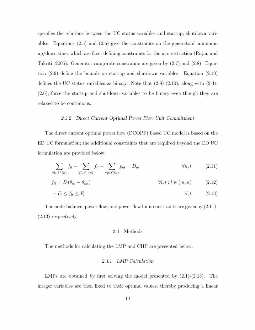
2.3.2 Direct Current Optimal Power Flow Unit Commitment

The direct current optimal power flow (DCOPF) based UC model is based on the

ED UC formulation; the additional constraints that are required beyond the ED UC

formulation are provided below.∑∀l∈δ+(n)

flt −∑

∀l∈δ−(n)

flt +∑∀g∈G(n)

pgt = Dnt ∀n, t (2.11)

flt = Bl(θnt − θmt) ∀l, t : l ∈ (m,n) (2.12)

− Fl ≤ flt ≤ Fl ∀, t (2.13)

The node-balance, power flow, and power flow limit constraints are given by (2.11)-

(2.13) respectively.

2.4 Methods

The methods for calculating the LMP and CHP are presented below.

2.4.1 LMP Calculation

LMPs are obtained by first solving the model presented by (2.1)-(2.13). The

integer variables are then fixed to their optimal values, thereby producing a linear

14

program. The LMPs are then the dual solution corresponding to the node-balance

constraint (2.11); note that for an ED model where there is no optimal power flow

formulation, the LMPs can be considered to come from the supply equals demand

constraint (2.2), which would give a single price to the entire system since the ED

structure assumes that there is a single bus. An alternative linear program can be

created by relaxing the integrality constraints on the commitment variables while

adding equality constraints that restrict them to their optimal values (Gribik et al.,

2007). For either formulation, the LMPs are the dual optimal solution associated to

the node-balance constraints.

2.4.2 CHP Calculation

CHPs are given by the slope of the convex hull of the total cost function within UC.

To determine the CHPs, the technique based on the Wang et al. (2012) ELMP model

is implemented. Lagrangian relaxation is applied to the node-balance constraints to

form the convex hull of the total cost function. The CHPs are then given by the

optimal Lagrange dual solution of the node-balance constraints.

In the following, the Lagrangian relaxation formulation is first provided; second,

the Lagrangian dual problem is shown to be a concave and piecewise linear function,

which allows the problem to be solved by using the subgradient algorithm; finally,

the decomposition method is introduced to simplify the problem into sub-problems

for each generator by relaxing the system node-balance constraints. Note that the

following derivation is for the ED UC model; however, the derivation also applies to

the DCOPF UC model.

15

Lagrangian Relaxation

Consider the ED UC model and apply Lagrangian relaxation by relaxing (2.2). Denote

the resulting Lagrangian dual optimal objective value as zLD, then zLD ≤ zEDUC ,

where zEDUC is the objective value of the ED UC problem (Bazaraa et al., 2006).

The Lagrangian dual problem is described as follows.

zLD = max zLR(λ)

where

zLR(λ) = min

[∑∀g

∑∀t

(CSUg vgt + CNL

g ugt + Cgpgt)−∑∀t

λt

(∑∀g

pgt −∑∀n

Dnt

)]

s.t. (2.3)− (2.10)

Concavity

Denote the feasible set of (2.3)-(2.10) as {pgt, ugt, vgt, wgt} ∈ Q. Note that conv(Q)

is a polytope since {pgt, ugt, vgt, wgt} are all bounded. Denote {pjgt, ujgt, v

jgt, w

jgt},∀j =

1, 2, · · · , J as the extreme points of conv(Q), then

zLR(λ) = min{f j(λ),∀j = 1, 2, · · · , J}

where f j(λ) =∑∀g∑∀t(CSUg vjgt + CNL

g ujgt + Cgpjgt

)−∑∀t λt

(∑∀g p

jgt −

∑∀nDnt

),∀j =

1, 2, · · · , J , since the minimum is obtained at the extreme points of conv(Q).

Proposition. zLR(λ) is a piecewise linear concave function.

Proof. Since, {pjgt, ujgt, v

jgt, w

jgt},∀j are fixed parameters, f j(λ) is a linear function of

λ. Moreover, zLR(λ) is the minimum of a finite set of linear functions f j(λ),∀j =

1, 2, · · · , J , thus, zLR(λ) is piecewise linear function with finite many break points.

16

For any two points λ1, λ2, let λ3 = αλ1 + (1 − α)λ2 be a convex combination of

λ1, λ2, where α ∈ (0, 1). Without loss of generality, suppose f j∗(λ3) is the minimum

function for λ3. Then

zLR(λ3) = f j∗(λ3)

= f j∗(αλ1 + (1− α)λ2)

= αf j∗(λ1) + (1− α)f j

∗(λ2)

≥ αmin{f j(λ1),∀j}+ (1− α) min{f j(λ2), ∀j}

That is,

zLR(αλ1 + (1− α)λ2) ≥ αzLR(λ1) + (1− α)zLR(λ2),∀α ∈ (0, 1)

Therefore, zLR(λ) is concave.

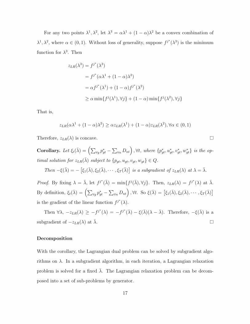
Corollary. Let ξt(λ) =(∑

∀g p∗gt −

∑∀nDnt

),∀t, where {p∗gt, u∗gt, v∗gt, w∗gt} is the op-

timal solution for zLR(λ) subject to {pgt, ugt, vgt, wgt} ∈ Q.

Then −ξ(λ) = −[ξ1(λ), ξ2(λ), · · · , ξT (λ)

]is a subgradient of zLR(λ) at λ = λ.

Proof. By fixing λ = λ, let f j∗(λ) = min{f j(λ), ∀j}. Then, zLR(λ) = f j

∗(λ) at λ.

By definition, ξt(λ) =(∑

∀g p∗gt −

∑∀nDnt

),∀t. So ξ(λ) =

[ξ1(λ), ξ2(λ), · · · , ξT (λ)

]is the gradient of the linear function f j

∗(λ).

Then ∀λ, −zLR(λ) ≥ −f j∗(λ) = −f j∗(λ) − ξ(λ)(λ − λ). Therefore, −ξ(λ) is a

subgradient of −zLR(λ) at λ.

Decomposition

With the corollary, the Lagrangian dual problem can be solved by subgradient algo-

rithms on λ. In a subgradient algorithm, in each iteration, a Lagrangian relaxation

problem is solved for a fixed λ. The Lagrangian relaxation problem can be decom-

posed into a set of sub-problems by generator.

17

By re-ordering the terms in zLR,

zLR = min[∑

∀g∑∀t(CSUg vgt + CNL

g ugt + Cgpgt − λtpgt)

+∑∀t λt (

∑∀nDnt)

]Denote zLR = min

∑∀g Lg +

∑∀t λt (

∑∀nDnt)

where Lg ≡∑∀g∑∀t(CSUg vgt + CNL

g ugt + Cgpgt − λtpgt).

The subprobelm zLRg(λ),∀g is defined as:

zLRg(λ) = min∑∀g

∑∀t

(CSUg vgt + CNL

g ugt + Cgpgt − λtpgt)

s.t. (2.3)− (2.10)

2.4.3 Subgradient Algorithm

The subgradient algorithm to find the optimal solution of λ, i.e. the CHP, is

described as follows.

Algorithm 1 Subgradient Algorithm

Initialize: i = 0, given λ(0)

repeati = i+ 1p(i) = solution of LR(λ(i−1))ξ(i) = solution of DR(p(i))λ(i) = λ(i−1) + β(i)ξ(i)

until ||λ(i) − λ(i−1)|| < εreturn λ(i)

LR(λ)for g ∈ G do

solve Lg(λ) get p∗gtend forreturn p

DR( ¯(p)for t ∈ T doξt =

∑∀g pgt −

∑∀nDnt

end forξ = ξ/||ξ||return ξ

β(i) is the step size for iteration i, which satisfies∑∞

i=1 β(i) =∞. limi→∞ β

(i) = 0

18

2.5 Test Results

In this chapter, a modified version of the IEEE RTS96 single zone model is used,

which consists of 24 buses, 33 generators, and 37 lines; the problem is formulated as

a day-ahead UC problem with 24 periods. Additional information can be found in

University of Washington (2015). The optimization is performed using IBM ILOG

CPLEX version 12.4 with Concert Technology version 3.6.

First, the uplift payments are examined under two pricing mechanisms for both

the ED UC and DCOPF UC models. In this chapter, the uplift payments are reserved

solely for generation participants facing negative profits. The uplift payments are then

socialized uniformly amongst the load according to the percent of total load.

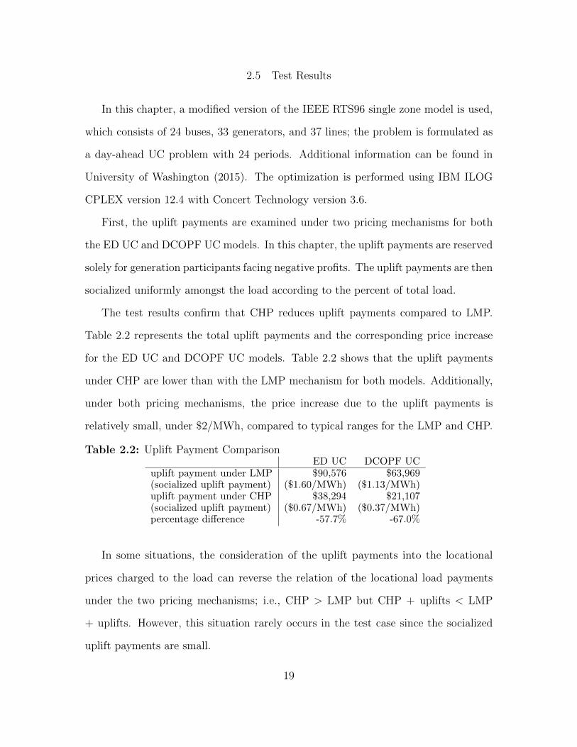
The test results confirm that CHP reduces uplift payments compared to LMP.

Table 2.2 represents the total uplift payments and the corresponding price increase

for the ED UC and DCOPF UC models. Table 2.2 shows that the uplift payments

under CHP are lower than with the LMP mechanism for both models. Additionally,

under both pricing mechanisms, the price increase due to the uplift payments is

relatively small, under $2/MWh, compared to typical ranges for the LMP and CHP.

Table 2.2: Uplift Payment ComparisonED UC DCOPF UC

uplift payment under LMP $90,576 $63,969(socialized uplift payment) ($1.60/MWh) ($1.13/MWh)uplift payment under CHP $38,294 $21,107(socialized uplift payment) ($0.67/MWh) ($0.37/MWh)percentage difference -57.7% -67.0%

In some situations, the consideration of the uplift payments into the locational

prices charged to the load can reverse the relation of the locational load payments

under the two pricing mechanisms; i.e., CHP > LMP but CHP + uplifts < LMP

+ uplifts. However, this situation rarely occurs in the test case since the socialized

uplift payments are small.

19

Next, the total load payment, generation cost, generation revenue, and generation

rent under LMP and CHP are examined for the ED UC and DCOPF UC models.

Table 2.3 and Table 2.4 represent the results for the ED UC and DCOPF UC models

respectively. Additionally, Table 2.4 gives the total congestion rent for the DCOPF

UC model. Note that the uplift payments are included in the total load payment,

generation revenue, and generation rent values calculation. The results show that the

total load payment, generation revenue, and generation rent are higher under CHP

than LMP for both the ED UC and DCOPF UC models. The total congestion rent in

the DCOPF UC model is increased under CHP as well. It is important to note that

the LMP and CHP mechanisms will not affect the operations in power systems as

both pricing mechanisms are based on the same UC and ED solutions. Thus, the total

generation cost and social welfare remain the same under each pricing mechanism as

only the allocation of wealth differs.

Table 2.3: Load Payment and Generation Rent Comparison under ED UCpercentage

LMP($) CHP($) differencetotal load payment 3,242,963 3,623,765 11.74%total generation revenue 3,242,963 3,623,765 11.74%total generation rent 2,203,858 2,584,660 17.28%total generation cost $ 1,039,104

Table 2.4: Load Payment and Generation Rent Comparison under DCOPF UCpercentage

LMP($) CHP($) differencetotal load payment 3,004,502 3,413,857 14.33%total generation revenue 2,113,497 2,378,503 12.54%total generation rent 999,625 1,264,631 26.51%total congestion rent 891,005 1,056,460 18.57%total generation cost $ 1,113,872

With the LMP pricing mechanism, existing simultaneous feasibility tests (SFT)

guarantee revenue adequacy for the financial transmission rights (FTR) market, un-

der a set of assumptions (Hogan, 1992); however, even with the same assumptions,

20

the CHP pricing mechanism does not guarantee revenue adequacy for the FTR mar-

kets. There is no guarantee that the congestion rent is sufficient to compensate the

FTR holders with the CHP pricing mechanism. It has been shown in Cadwalader

et al. (2010) that the duality gap between the optimal values of the Lagrangian dual

problem and the UC problem serves as an upper bound on the funds required to

incentivize the market solution and includes the funds required to guarantee revenue

adequacy for the FTR market.

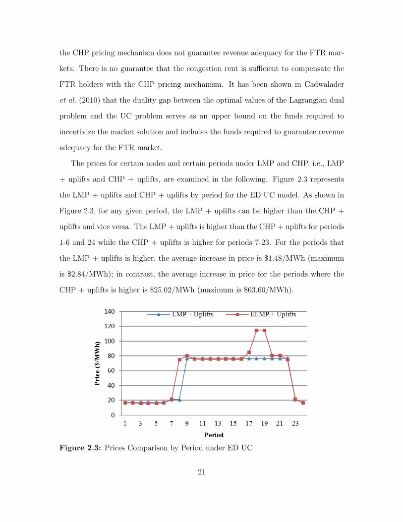
The prices for certain nodes and certain periods under LMP and CHP, i.e., LMP

+ uplifts and CHP + uplifts, are examined in the following. Figure 2.3 represents

the LMP + uplifts and CHP + uplifts by period for the ED UC model. As shown in

Figure 2.3, for any given period, the LMP + uplifts can be higher than the CHP +

uplifts and vice versa. The LMP + uplifts is higher than the CHP + uplifts for periods

1-6 and 24 while the CHP + uplifts is higher for periods 7-23. For the periods that

the LMP + uplifts is higher, the average increase in price is $1.48/MWh (maximum

is $2.84/MWh); in contrast, the average increase in price for the periods where the

CHP + uplifts is higher is $25.02/MWh (maximum is $63.60/MWh).

Figure 2.3: Prices Comparison by Period under ED UC

21

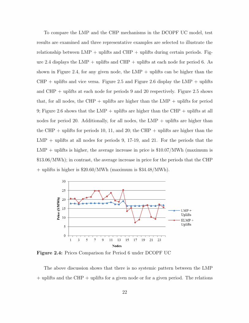
To compare the LMP and the CHP mechanisms in the DCOPF UC model, test

results are examined and three representative examples are selected to illustrate the

relationship between LMP + uplifts and CHP + uplifts during certain periods. Fig-

ure 2.4 displays the LMP + uplifts and CHP + uplifts at each node for period 6. As

shown in Figure 2.4, for any given node, the LMP + uplifts can be higher than the

CHP + uplifts and vice versa. Figure 2.5 and Figure 2.6 display the LMP + uplifts

and CHP + uplifts at each node for periods 9 and 20 respectively. Figure 2.5 shows

that, for all nodes, the CHP + uplifts are higher than the LMP + uplifts for period

9; Figure 2.6 shows that the LMP + uplifts are higher than the CHP + uplifts at all

nodes for period 20. Additionally, for all nodes, the LMP + uplifts are higher than

the CHP + uplifts for periods 10, 11, and 20; the CHP + uplifts are higher than the

LMP + uplifts at all nodes for periods 9, 17-19, and 21. For the periods that the

LMP + uplifts is higher, the average increase in price is $10.07/MWh (maximum is

$13.06/MWh); in contrast, the average increase in price for the periods that the CHP

+ uplifts is higher is $20.60/MWh (maximum is $34.48/MWh).

Figure 2.4: Prices Comparison for Period 6 under DCOPF UC

The above discussion shows that there is no systemic pattern between the LMP

+ uplifts and the CHP + uplifts for a given node or for a given period. The relations

22

Figure 2.5: Prices Comparison for Period 9 under DCOPF UC

Figure 2.6: Prices Comparison for Period 20 under DCOPF UC

of the two prices vary with different nodes and different periods.

Finally, the price sensitivity based on the change of loads is examined. The test

results show that, with congestion, the CHP + uplifts is no longer a monotonically

non-decreasing function with respect to the load. Figure 2.7 shows one instance

at node 1 for period 17. The non-monotonicity is caused by the congestion in the

network. One of the main arguments in support of the CHP is that it creates a

monotonically nondecreasing function with respect to the load for economic dispatch

(with unit commitment) problems, as shown in Gribik et al. (2007). Frequently, the

marginal cost to produce a good increases as one wishes to produce more and, thus,

23

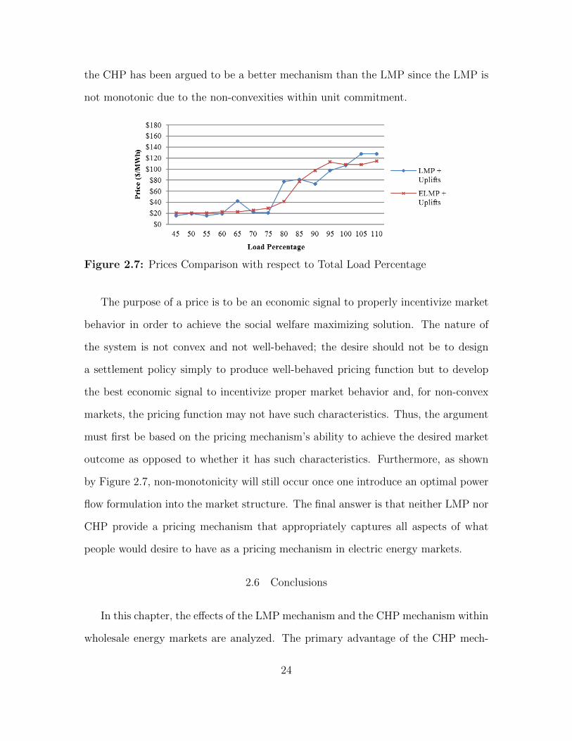
the CHP has been argued to be a better mechanism than the LMP since the LMP is

not monotonic due to the non-convexities within unit commitment.

Figure 2.7: Prices Comparison with respect to Total Load Percentage

The purpose of a price is to be an economic signal to properly incentivize market

behavior in order to achieve the social welfare maximizing solution. The nature of

the system is not convex and not well-behaved; the desire should not be to design

a settlement policy simply to produce well-behaved pricing function but to develop

the best economic signal to incentivize proper market behavior and, for non-convex

markets, the pricing function may not have such characteristics. Thus, the argument

must first be based on the pricing mechanism’s ability to achieve the desired market

outcome as opposed to whether it has such characteristics. Furthermore, as shown

by Figure 2.7, non-monotonicity will still occur once one introduce an optimal power

flow formulation into the market structure. The final answer is that neither LMP nor

CHP provide a pricing mechanism that appropriately captures all aspects of what

people would desire to have as a pricing mechanism in electric energy markets.

2.6 Conclusions

In this chapter, the effects of the LMP mechanism and the CHP mechanism within

wholesale energy markets are analyzed. The primary advantage of the CHP mech-

24

anism is that uplift payments are minimized. However, by incorporating fixed costs

into the locational uniform price, the CHP is not a market clearing price for the mar-

ket dispatch solution, which is an important advantage of the LMP mechanism. The

results show that the CHPs + uplifts can be higher or lower than the LMPs + uplifts

at each node. Additionally, the total load payment, generation revenue, and genera-

tion rent are increased under CHP over LMP for both the ED UC and DCOPF UC

models. The total congestion rent in the DCOPF UC model is also increased under

CHP. Furthermore, because CHP is not a market clearing price for the market dis-

patch solution, the simultaneous feasibility test does not guarantee revenue adequacy

for the FTR market.

Implementing the convex hull pricing takes much more efforts since solving the

dual of a mixed integer problem (MIP) is extremely hard. Few RTO/ISO have been

convinced to switch to the convex hull pricing even though they understand the issues

of standard LMP. Although CHP scheme minimizes the amount uplift payment, the

uplift payment is not eliminated under this scheme since the duality gap of MIP.

At this time, it is difficult to conclude that CHP is outright the preferred mecha-

nism. Further studies are needed to confirm how the CHP mechanism will affect the

load payment and the generation rent as compared to the LMP pricing mechanism.

A better pricing scheme is desired but it may not solve all potential issues in DAM.

25

Chapter 3

STOCHASTIC DISPATCHABLE PRICING

3.1 Introduction

A well-designed pricing scheme should provide a proper pricing signal and be

incentive compatible. The currently utilized locational marginal price scheme releases

a proper pricing signal for dispatch, but fails to capture commitment costs. Moreover,

price inconsistency exists between day-ahead and real-time markets under the current

deterministic pricing scheme. As more intermittent renewable resources are being

introduced to power grids, the inconsistency is expected to be amplified.

Currently, two-thirds of the population in the U.S. is served by an Independent

System Operator (ISO) or Regional Transmission Organization (RTO) for whole-

sale electricity trades. The ISO/RTOs coordinate system operations with different

markets and services including but not limited to energy markets, financial transmis-

sion rights markets, capacity markets, ancillary services, and congestion management

(California ISO, 2015). Those markets and services are designed with the goal of

being incentive compatible (i.e., to induce all participants to truthfully reveal private

information and have no incentive to deviate from market solutions) in order to bring

competition and ultimately to maximize social welfare (producer surplus, consumer

surplus and congestion rent). Electricity differs from ordinary products in several

ways: demand is close to perfectly inelastic; supply and demand must be in balance

to maintain system frequency continuously under high uncertainty; electricity travels

in the power grid with very fast speed and follows Kirchhoff’s laws; storage is usually

considered too expensive with current technologies; most generators take some time

26

to start up and shut down, and once they are on or off, they need to stay on or off for

minimum up and down times. Due to the unique nature of the electricity commodity,

pricing schemes play a very important role in electricity market design.

A well-designed pricing scheme should release proper pricing signals and induce

participants’ behavior to maximize social welfare. The term, pricing signal, is used

to describe the forward informational value of the market clearing price that is used

to settle the market.

The focus of this chapter is on pricing schemes in day-ahead energy markets

(DAM). The analysis here does not consider the potential exercise of market power

and assumes all participants behave non-strategically. The analysis focuses on pricing

signals under different pricing schemes.

The current locational marginal pricing (LMP) scheme in DAM, referred to as

restricted LMP from now on, is described as follows. The ISO/RTO first solves a

security-constrained unit commitment (SCUC) problem based on the bids from both

the supply and demand sides. The solution from SCUC try to ensure that enough

generators will be turned on to maintain system reliability under uncertainty while

keeping economic efficiency at the same time. Then, by fixing the unit commitments,

a security-constrained economic dispatch (SCED) model with network constraints is

solved, and LMPs are obtained as the dual variables of node-balance constraints. The

dual variable represents the change in the objective (total economic surplus) when

a small amount increment/decrement of power is consumed at the corresponding

location. It releases a proper pricing signal for the marginal cost of dispatch.

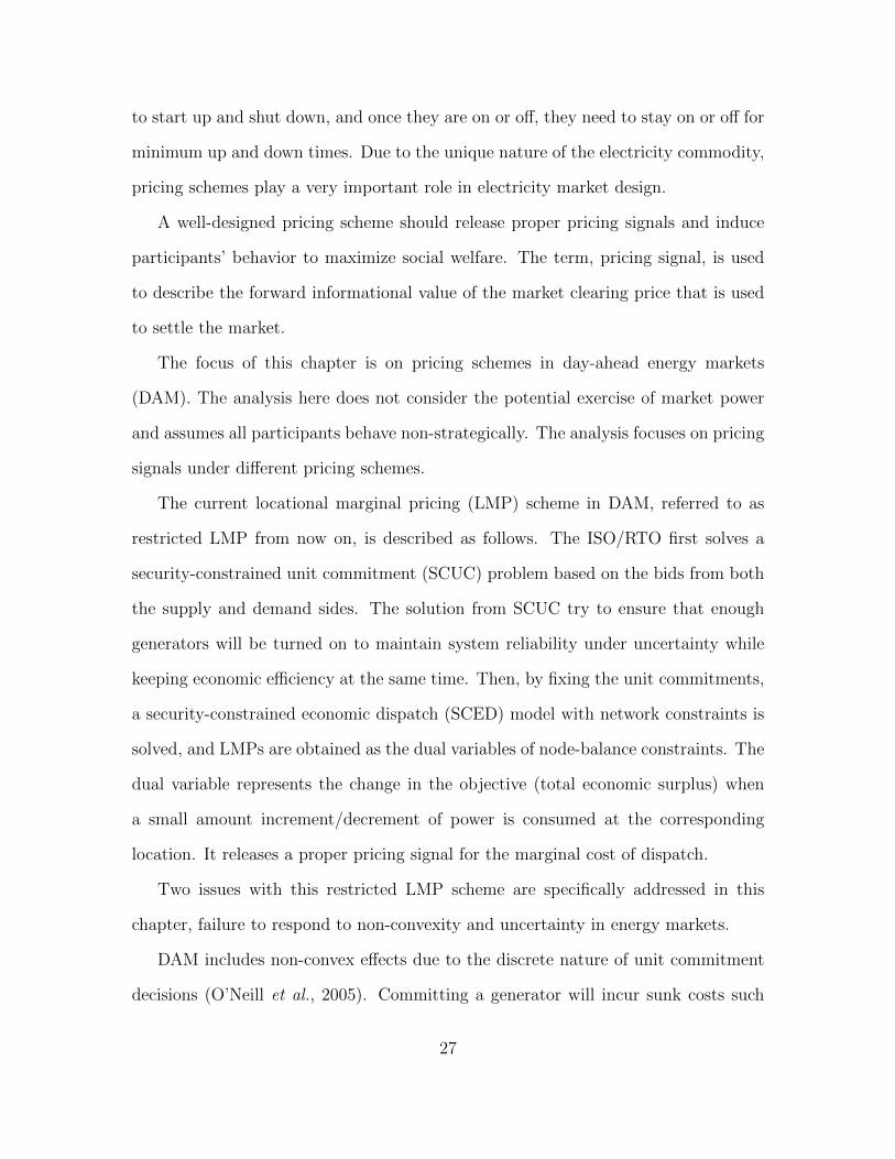
Two issues with this restricted LMP scheme are specifically addressed in this

chapter, failure to respond to non-convexity and uncertainty in energy markets.

DAM includes non-convex effects due to the discrete nature of unit commitment

decisions (O’Neill et al., 2005). Committing a generator will incur sunk costs such

27

as startup cost and no-load cost. Moreover, minimum generation requirements and

minimum up and down time constraints also contribute to the non-convexities. Since

the restricted LMP does not take commitment costs into consideration, a generator’s

revenue may not be sufficient to cover all its costs. Then, the ISO/RTO pays the

generator uplift payments to bring its negative net profit to zero, thereby giving the

generator an incentive to commit according to the DAM schedule (O’Neill et al.,

2005). On the other hand, if the market price is higher than a generator’s marginal

cost, the generator has incentive to produce to EcoMax in order to maximize profits.

If the market solution instructs the generator to dispatch under EcoMax, then lost

opportunity cost uplift payment is paid to compensate the mis-incentives. Gribik

et al. (2007) proposed a convex hull pricing (CHP) scheme, which takes the dual of

the entire unit commitment model, setting prices as the Lagrange multipliers of node-

balance constraints. The CHP aims at giving better pricing signals than the restricted

LMP. Gribik et al. (2007) proved that CHP minimizes uplift payments. Moreover,

it gives a monotonically non-decreasing marginal cost function with respect to total

loads, whereas the restricted LMP does not. In order to calculate CHPs, the dual

problem of a mixed integer programing needs to be solved, which is computationally

difficult. Gribik et al. (2007) also discussed a dispatchable model. For a single-bus,

single-period model, Gribik et al. (2007) showed that the prices under the dispatchable

model are the same as that under CHP, by relaxing generation minimum requirement

constraints and allocating fixed cost to generation variable cost. The ISO/RTOs have

implemented modifications based on the restricted LMP to reduce uplift payments.

Most ISO/RTOs amortize startup and no-load costs to generation variable cost to set

generation marginal cost (Federal Energy Regulatory Commission, 2014a). Moreover,

some ISO/RTOs allow committed inflexible fast-start generators to set energy prices

although they cannot change their dispatch. Several ISO/RTOs, such as ISO-NE,

28

NYISO, MISO, allow off-line fast-start units to set energy prices (Federal Energy

Regulatory Commission, 2014a). Although many efforts have been devoted to deal

with uplift payments, no method claims to eliminate uplift payments completely. In

fact, Gribik (2007) states that the discrete nature of commitment decisions, startup

costs, and no-load costs may prevent the existence of an efficient market clearing

price in DAM since there is generally no set of market prices that would induce profit

maximizing generators and loads to voluntarily follow the pricing scheme.

Standard energy markets’ setup has both DAM and a real-time energy market

(RTM). When designing pricing schemes for DAM, its impacts on RTM should be

considered jointly. The restricted LMP adopts a deterministic model, i.e., taking

expected or forecasted values of uncertain parameters as input data. Zavala et al.

(2014) demonstrated and proved that price inconsistency exists between DAM and

RTM with the restricted LMP. In other words, the expected RTM price differs from

the DAM price. Market manipulation could happen if a participant sees persistent

price premia between RTM and DAM, which consequently can cause problems such

as revenue inadequacy (Zavala et al., 2014). Therefore, a deterministic model that

is based on summarizing statistics will not result in an efficient pricing scheme un-

der high uncertainty: hence, a stochastic model is desired. Pritchard et al. (2010)

and Morales et al. (2012) studied stochastic pricing schemes. The stochastic pricing

scheme is usually a two-stage model, where the first stage represents DAM and the

second stage simulates RTM. In the second stage, a set of plausible scenarios are

included as predicted scenarios of RTM. Stochastic pricing schemes can be seen as a

methodology to smooth LMP changes in DAM. Under the restricted LMP, at some

load points, the LMP “jumps” dramatically. Under stochastic pricing schemes, DAM

energy prices are still set as the dual variables of the node-balance constraints; how-

ever, by including plausible RTM scenarios, the returned prices are consistent with

29

RTM prices and price gaps are reduced.

In this chapter, a new pricing scheme in DAM is proposed by relaxing constraints

that cause non-convexities and adopting a stochastic pricing formulation simultane-

ously. The proposed pricing scheme has the following advantages: 1) it addresses

both non-convexities and uncertainty issues in DAM, and none of the existing liter-

ature has studied these two issues jointly; 2) the pricing run can be separated from

unit commitments; 3) the resulting marginal price is a monotonically non-decreasing

function with respect to total loads; 4) reduced uplift payments; 5) low computational

complexity.

The rest of the chapter is organized as follows. Section 3.2 gives the mathematical

model of the proposed new pricing scheme. Section 3.3 demonstrates two test case

results. Finally, Section 3.4 concludes the chapter.

3.2 Pricing Model

In this section, the proposed pricing model is given first, followed by the explana-

tion and analysis of the model.

30

3.2.1 Model Overview

min∑∀s:s 6=0

πs∑∀t

[∑∀g

(CMg p

sgt + δg∆p

sgt) +

∑∀j

(Cjwsjt + ηj∆w

sjt)

](3.1)

s.t. 0 ≤ psgt ≤ Pmaxg ∀g, t, s (3.2)

0 ≤ wsjt ≤ W sjt ∀j, t, s (3.3)∑

∀g∈G(n)

p0gt +∑∀j∈J(n)

w0jt − i0nt = Dnt ∀n, t (λnt) (3.4)

∑∀g∈G(n)

(psgt − p0gt) +∑∀j∈J(n)

(wsjt − w0jt)− (isnt − i0nt) = 0

∀n, t, s : s 6= 0 (πsµsnt) (3.5)∑∀n

isnt = 0 ∀t, s (3.6)

− Fl ≤∑∀n

ψnlisnt ≤ Fl ∀l, t, s (3.7)

psgt − psg,t−1 ≤ Rhrg ∀g, t, s (3.8)

psg,t−1 − psgt ≤ Rhrg ∀g, t, s (3.9)

∆psgt ≥ psgt − p0gt ∀g, t, s : s 6= 0 (3.10)

∆psgt ≥ p0gt − psgt ∀g, t, s : s 6= 0 (3.11)

∆wsjt ≥ wsjt − w0jt ∀j, t, s : s 6= 0 (3.12)

∆wsjt ≥ w0jt − wsjt ∀j, t, s : s 6= 0 (3.13)

0 ≤ psgt ≤ Qg ∀g, t, s : s 6= 0 (3.14)

∆wsjt ≥ 0 ∀j, t, s : s 6= 0 (3.15)

The problem is formulated as a 24-period day-ahead model with uncertainty. The

uncertainty in this pricing model represents the intermittent wind power generation

in power grids, i.e., the realized available wind generation capacity W sjt in the real-

31

time scenarios. The model adopts a direct current optimal power flow (DCOPF)

formulation. Equation (3.1) is the objective function that minimizes the expected

scenario-based dispatch costs. Equation (3.2) is the generation level constraint for

traditional generators. Equation (3.3) is the generation level constraint for wind

farms. Equation (3.4) is the node-balance constraint for the base case. Equation

(3.5) is the node-balance constraint for plausible real-time scenarios. Equation (3.6)

is the total injection constraint. Equation (3.7) restricts transmission line flows.

Equations (3.8) and (3.9) specify hourly ramping rate constraints. Equations (3.10)-

(3.15) specify the generation deviation between base case and plausible scenarios.

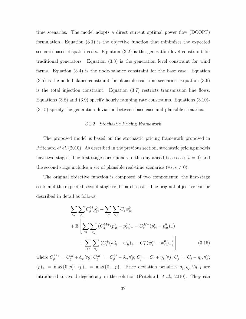
3.2.2 Stochastic Pricing Framework

The proposed model is based on the stochastic pricing framework proposed in

Pritchard et al. (2010). As described in the previous section, stochastic pricing models

have two stages. The first stage corresponds to the day-ahead base case (s = 0) and

the second stage includes a set of plausible real-time scenarios (∀s, s 6= 0).

The original objective function is composed of two components: the first-stage

costs and the expected second-stage re-dispatch costs. The original objective can be

described in detail as follows.∑∀t

∑∀g

CMg p

0gt +

∑∀t

∑∀j

Cjw0jt

+ E

[∑∀t

∑∀g

(CM+g (psgt − p0gt)+ − CM−

g (psgt − p0gt)−)

+∑∀t

∑∀j

(C+j (wsjt − w0

jt)+ − C−j (wsjt − w0jt)−

)](3.16)

where CM+g = CM

g + δg,∀g; CM−g = CM

g − δg,∀g; C+j = Cj + ηj, ∀j; C−j = Cj − ηj,∀j;

(p)+ = max{0, p}; (p)− = max{0,−p}. Price deviation penalties δg, ηj,∀g, j are

introduced to avoid degeneracy in the solution (Pritchard et al., 2010). They can

32

be seen as penalty prices for the generation deviation from base case and plausible

real-time scenarios. For instance, assume the planned generation for a generator is

100MW with marginal cost $10/MWh in DAM. If there is a price penalty $0.1/MWh,

when demand is 110MW, the generator can sell 10MW more in RTM with marginal

price $10.1/MWh. If demand is 90MW, the generator buys back 10MW with marginal

price $9.9/MWh. The penalty prices help to avoid the existence of non-unique dual

solutions, i.e., degenerate solutions. After simplification, the objective is equivalent

to:

E

[∑∀t

∑∀g

(CMg p

sgt + δg|psgt − p0gt|

)+∑∀t

∑∀j

(Cjw

sjt + ηj|wsjt − w0

jt|)]

(3.17)

Then, by linearizing the absolute values with (3.10)-(3.13), the objective is represented

as (3.1).

Price deviation penalties connect the dispatch decisions between the first-stage

base case and second-stage scenarios. The DAM prices under stochastic pricing are set

to be the dual variables of the node-balance constraint of the base case, i.e., the dual

variable λnt of (3.4). The dual variable of (3.5) is the product of the corresponding

plausible scenario’s probability and LMP, µsnt (Pritchard et al., 2010). Wong and

Fuller (2007) proved that µsnt are also dual optimal for each single scenario. In other

words, µsnt are real-time LMPs for the corresponding scenarios if the plausible scenario

is realized. It can be proved that λnt =∑∀s π

sµsnt,∀n, t (Pritchard et al., 2010).

Therefore, under the stochastic pricing scheme, DAM LMPs are consistent with RTM

LMPs in expectation, for the given set of plausible real-time scenarios. From another

perspective, the resulting DAM LMPs under the stochastic LMP are smoother than

under the deterministic pricing scheme, as the prices are averages of all plausible

scenarios. The LMP function with respect to total loads is no longer a step-size

function but is close to a continuous function. This result will be further discussed

33

with test cases in the next section.

3.2.3 Dispatchable Relaxation

Current restricted LMPs are obtained by fixing unit commitment solutions and

then solving the economic dispatch model. The discrete nature of unit commitment

causes LMPs to change non-monotonically with respect to total loads. At some load

point, a new committed unit may increase or decrease the marginal cost of dispatch.

From an economic point of view, more demand should result in higher prices. The

restricted LMP does not provide a good pricing signal in the sense that it results in

non-monotonic prices with respect to total loads. In addition, uplift payments are

required since the restricted LMP does not take commitment costs into consideration.

The proposed pricing scheme aims at eliminating the non-convexity of energy markets

and giving better pricing signals with the following modifications.

First, commitment costs are amortized to generation variable costs to reduce uplift

payments as follows.

CMg = Cg + CNL

g /Pmaxg + CSU

g /UTg/Pmaxg (3.18)

Both no-load costs and startup costs are allocated to generation variable costs.

The no-load cost is allocated to each generator up to their maximum generation levels,

assuming every MW of capacity contributes to the no-load cost. Once a generator is

turned on, the startup cost incurs. Then, the generator has to be on for the minimum

up time. Thus, the startup cost is allocated to variable generation cost divided by

minimum up time and maximum generation level. Other amortization rules may be

adopted, but they are left for future study.

Next, the minimum generation levels of all units are relaxed to zero. The idea

is inherited from the dispatchable model in Gribik et al. (2007). In this chapter,

34

the model is extended to a multi-period model with network constraints. The dis-

patchable assumption modification matches current industry practice in the U.S. For

instance, most ISO/RTOs relax fast-start generators’ minimum generation levels to

zero, thereby allowing them to set prices, and some ISO/RTOs also allow uncommit-

ted fast start units to set the RTM price (Federal Energy Regulatory Commission,

2014a). In the proposed DAM pricing model, all units are assumed dispatchable,

including committed and uncommitted fast- and slow-starting units.

There are several implications from these modifications. Firstly, by assuming all

units to be dispatchable, the non-convexity issues are eliminated. The resulting LMP

increases monotonically as total loads increase. Secondly, the pricing model is sep-

arated from unit commitment. Consequently, the pricing run can be carried out in

parallel with SCUC and SCED. Thirdly, uplift payments are reduced. The above two

modifications result in prices that are close to CHP (i.e., minimizing uplift payments).

In place of theoretical justification, this chapter studies test cases and compares up-

lift payments under the proposed pricing model and the restricted LMP under more

realistic assumptions. In the next section, test case results confirm that the uplift

payments under the proposed pricing model are indeed reduced. Although uplift

payments are reduced, they are not totally eliminated. When a generator dispatches

under its full capacity, commitment costs may not be fully recovered. Equation (3.18)

is an approximation to recover commitment costs that assumes maximum generation.

As mentioned previously, the complex nature of electric power energy markets pre-

vents the existence of prices in equilibrium where all participants will voluntarily

follow dispatch instructions.

35

3.2.4 DAM and RTM Process

The proposed model is a pricing model to determine the energy prices in DAM.

The dispatch solutions from this pricing model will possibly be different from the

SCED solution since all units are relaxed to be dispatchable. However, the obtained

LMPs from the pricing model are utilized for financial settlements and market surplus

allocation. The DAM commitment and dispatch schedules are still determined by

SCUC and SCED. This structure follows the ISO/RTOs’ practice where they relax

fast-start generators’ minimum generation levels to zero in pricing models to set

prices, though they are inflexible (i.e., the minimum generation requirement equals

to the maximum generation requirement for gas turbines) Federal Energy Regulatory

Commission (2014a).

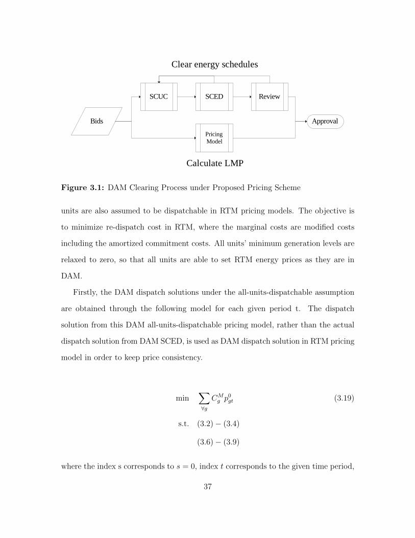
In general, the current DAM clearing process can be seen as collecting bids, solv-

ing SCUC, solving SCED, solving the pricing model, adding reliability corrections

(if needed), and finally settling the market. Under the proposed pricing scheme, all

generators are included in the model to set energy prices. This is in contrast to the

restricted LMP where only committed units can set prices. As a result of relaxing all

units to be dispatchable, one advantage of the proposed pricing scheme is that the

pricing run is separated from SCUC, i.e., the pricing model is independent of com-

mitment solutions. Solving the pricing model only requires the bidding information

such as commitment costs, dispatch variable costs and total capacities. Figure 3.1

represents the new DAM clearing process under the proposed pricing scheme. The

pricing run is in parallel with SCUC and SCED. This structure enables ISO/RTOs

to have more flexibility to solve stochastic pricing models, which generally take more

time to solve.

In order to keep price consistency with the proposed DAM pricing scheme, all

36

Bids

SCUC SCED Review

Pricing

Model

Approval

Clear energy schedules

Calculate LMP

Figure 3.1: DAM Clearing Process under Proposed Pricing Scheme

units are also assumed to be dispatchable in RTM pricing models. The objective is

to minimize re-dispatch cost in RTM, where the marginal costs are modified costs

including the amortized commitment costs. All units’ minimum generation levels are

relaxed to zero, so that all units are able to set RTM energy prices as they are in

DAM.

Firstly, the DAM dispatch solutions under the all-units-dispatchable assumption

are obtained through the following model for each given period t. The dispatch

solution from this DAM all-units-dispatchable pricing model, rather than the actual

dispatch solution from DAM SCED, is used as DAM dispatch solution in RTM pricing

model in order to keep price consistency.

min∑∀g

CMg p

0gt (3.19)

s.t. (3.2)− (3.4)

(3.6)− (3.9)

where the index s corresponds to s = 0, index t corresponds to the given time period,

37

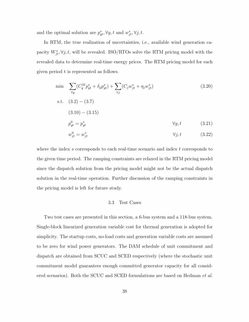
and the optimal solution are p∗gt,∀g, t and w∗jt,∀j, t.

In RTM, the true realization of uncertainties, i.e., available wind generation ca-

pacity W sjt,∀j, t, will be revealed. ISO/RTOs solve the RTM pricing model with the

revealed data to determine real-time energy prices. The RTM pricing model for each

given period t is represented as follows.

min∑∀g

(CMg p

sgt + δgp

sgt) +

∑∀j

(Cjwsjt + ηjw

sjt) (3.20)

s.t. (3.2)− (3.7)

(3.10)− (3.15)

p0gt = p∗gt ∀g, t (3.21)

w0jt = w∗jt ∀j, t (3.22)

where the index s corresponds to each real-time scenario and index t corresponds to

the given time period. The ramping constraints are relaxed in the RTM pricing model

since the dispatch solution from the pricing model might not be the actual dispatch

solution in the real-time operation. Further discussion of the ramping constraints in

the pricing model is left for future study.

3.3 Test Cases

Two test cases are presented in this section, a 6-bus system and a 118-bus system.

Single-block linearized generation variable cost for thermal generation is adopted for

simplicity. The startup costs, no-load costs and generation variable costs are assumed

to be zero for wind power generators. The DAM schedule of unit commitment and

dispatch are obtained from SCUC and SCED respectively (where the stochastic unit

commitment model guarantees enough committed generator capacity for all consid-

ered scenarios). Both the SCUC and SCED formulations are based on Hedman et al.

38

(2010). 10 wind power scenarios for the 6-bus system are obtained from Wang et al.

(2008). The available wind power scenarios for the 118-bus system are generated from

normal distributions and assigned with equal probability. This is a simple assumption

and alternative approaches are possible, but scenario generation and selection issues

are beyond the scope of this chapter. Penalty factor δg is set to be $0.1 for conven-

tional generators and penalty factor ηj is set to be $0.001 for wind farms, following

the rule in Zavala et al. (2014). DAM uplift payments are paid whenever a genera-

tor’s total payment is less than its total cost in 24 hours, following the convention in

Federal Energy Regulatory Commission (2014b).

Four pricing schemes are compared. Let DR represent the deterministic restricted

LMP scheme; SR represent the stochastic restricted LMP scheme; DA represent the

deterministic all-units-dispatchable LMP scheme; and SA represent the stochastic

all-units-dispatchable LMP scheme. The deterministic (D) pricing scheme does not

include any real-time scenarios; the stochastic (S) pricing scheme adopts the two-

stage stochastic pricing framework described in subsection III.B; the restricted (R)

pricing scheme fixes commitment solutions, allows only committed units to set energy

prices and uses variable generation costs (not including amortized commitment costs);

the all-units-dispatchable (A) pricing scheme adopts the modifications described in

subsection 3.2.3.

3.3.1 6-Bus System

The data of this system is modified from that presented in Wang et al. (2008).

The original data can be found in University of Washington (2015). All ten scenarios

in Wang et al. (2008) are included in the stochastic pricing scheme. The generator

data is shown in Table 3.1 and Table 3.2. Gen1 is a base-load generator since it has

lower generation variable cost and higher capacity. Gen2 is an expensive generator

39

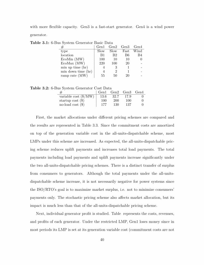
with more flexible capacity. Gen3 is a fast-start generator. Gen4 is a wind power

generator.

Table 3.1: 6-Bus System Generator Basic Data# Gen1 Gen2 Gen3 Gen4type Slow Slow Fast Windlocation B1 B2 B6 B4EcoMin (MW) 100 10 10 0EcoMax (MW) 220 100 20 -min up time (hr) 4 3 1 -min down time (hr) 4 2 1 -ramp rate (MW) 55 50 20 -

Table 3.2: 6-Bus System Generator Cost Data# Gen1 Gen2 Gen3 Gen4variable cost ($/MW) 13.6 32.7 17.9 0startup cost ($) 100 200 100 0no-load cost ($) 177 130 137 0

First, the market allocations under different pricing schemes are compared and

the results are represented in Table 3.3. Since the commitment costs are amortized

on top of the generation variable cost in the all-units-dispatchable scheme, most

LMPs under this scheme are increased. As expected, the all-units-dispatchable pric-

ing scheme reduces uplift payments and increases total load payments. The total

payments including load payments and uplift payments increase significantly under

the two all-units-dispatchable pricing schemes. There is a distinct transfer of surplus

from consumers to generators. Although the total payments under the all-units-

dispatchable scheme increase, it is not necessarily negative for power systems since

the ISO/RTO’s goal is to maximize market surplus, i.e. not to minimize consumers’

payments only. The stochastic pricing scheme also affects market allocation, but its

impact is much less than that of the all-units-dispatchable pricing scheme.

Next, individual generator profit is studied. Table represents the costs, revenues,

and profits of each generator. Under the restricted LMP, Gen1 loses money since in

most periods its LMP is set at its generation variable cost (commitment costs are not

40

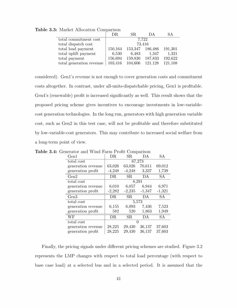
Table 3.3: Market Allocation ComparisonDR SR DA SA

total commitment cost 7,722total dispatch cost 73,416total load payment 150,164 153,347 186,486 191,301total uplift payment 6,530 6,483 1,347 1,321total payment 156,694 159,830 187,833 192,622total generation revenue 103,416 104,606 121,128 121,108

considered). Gen1’s revenue is not enough to cover generation costs and commitment

costs altogether. In contrast, under all-units-dispatchable pricing, Gen1 is profitable.

Gen4’s (renewable) profit is increased significantly as well. This result shows that the

proposed pricing scheme gives incentives to encourage investments in low-variable-

cost generation technologies. In the long run, generators with high generation variable

cost, such as Gen2 in this test case, will not be profitable and therefore substituted

by low-variable-cost generators. This may contribute to increased social welfare from

a long-term point of view.

Table 3.4: Generator and Wind Farm Profit ComparisonGen1 DR SR DA SAtotal cost 67,273generation revenue 63,026 63,026 70,611 69,012generation profit -4,248 -4,248 3,337 1,739

Gen2 DR SR DA SAtotal cost 8,291generation revenue 6,010 6,057 6,944 6,971generation profit -2,282 -2,235 -1,347 -1,321

Gen3 DR SR DA SAtotal cost 5,573generation revenue 6,155 6,093 7,436 7,523generation profit 582 520 1,863 1,949

WF DR SR DA SAtotal cost 0generation revenue 28,225 29,430 36,137 37,603generation profit 28,225 29,430 36,137 37,603

Finally, the pricing signals under different pricing schemes are studied. Figure 3.2

represents the LMP changes with respect to total load percentage (with respect to

base case load) at a selected bus and in a selected period. It is assumed that the

41

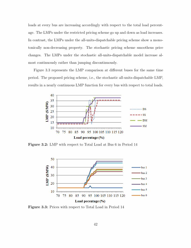
loads at every bus are increasing accordingly with respect to the total load percent-

age. The LMPs under the restricted pricing scheme go up and down as load increases.

In contrast, the LMPs under the all-units-dispatchable pricing scheme show a mono-

tonically non-decreasing property. The stochastic pricing scheme smoothens price

changes. The LMPs under the stochastic all-units-dispatchable model increase al-

most continuously rather than jumping discontinuously.

Figure 3.3 represents the LMP comparison at different buses for the same time

period. The proposed pricing scheme, i.e., the stochastic all-units-dispatchable LMP,

results in a nearly continuous LMP function for every bus with respect to total loads.

Figure 3.2: LMP with respect to Total Load at Bus 6 in Period 14

Figure 3.3: Prices with respect to Total Load in Period 14

42

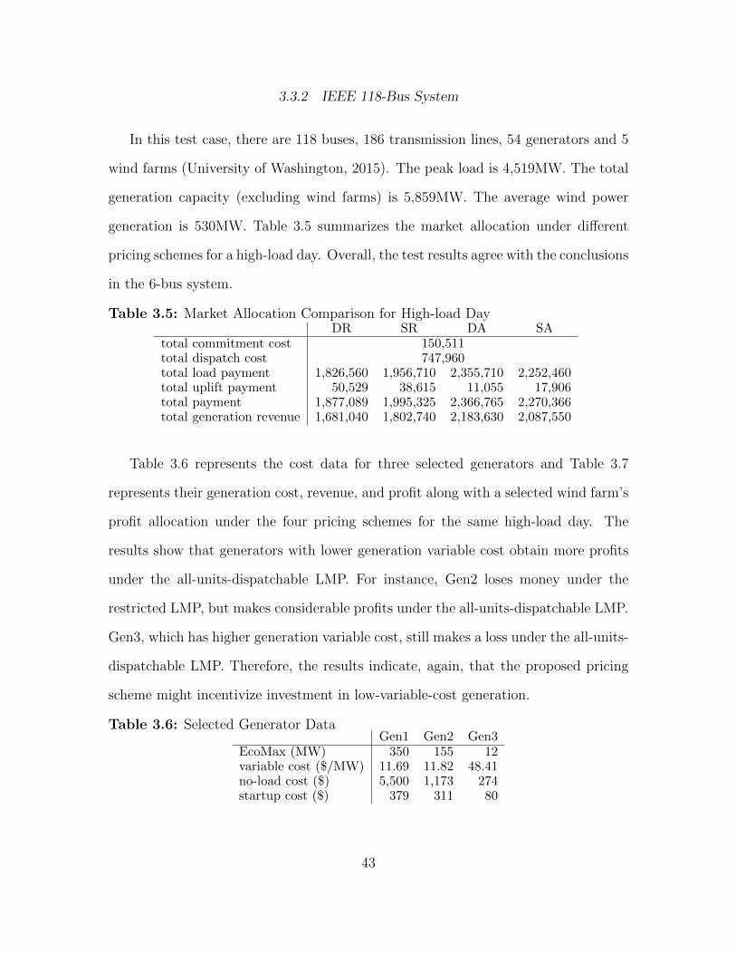
3.3.2 IEEE 118-Bus System

In this test case, there are 118 buses, 186 transmission lines, 54 generators and 5

wind farms (University of Washington, 2015). The peak load is 4,519MW. The total

generation capacity (excluding wind farms) is 5,859MW. The average wind power

generation is 530MW. Table 3.5 summarizes the market allocation under different

pricing schemes for a high-load day. Overall, the test results agree with the conclusions

in the 6-bus system.

Table 3.5: Market Allocation Comparison for High-load DayDR SR DA SA

total commitment cost 150,511total dispatch cost 747,960total load payment 1,826,560 1,956,710 2,355,710 2,252,460total uplift payment 50,529 38,615 11,055 17,906total payment 1,877,089 1,995,325 2,366,765 2,270,366total generation revenue 1,681,040 1,802,740 2,183,630 2,087,550

Table 3.6 represents the cost data for three selected generators and Table 3.7

represents their generation cost, revenue, and profit along with a selected wind farm’s

profit allocation under the four pricing schemes for the same high-load day. The

results show that generators with lower generation variable cost obtain more profits

under the all-units-dispatchable LMP. For instance, Gen2 loses money under the

restricted LMP, but makes considerable profits under the all-units-dispatchable LMP.

Gen3, which has higher generation variable cost, still makes a loss under the all-units-

dispatchable LMP. Therefore, the results indicate, again, that the proposed pricing

scheme might incentivize investment in low-variable-cost generation.

Table 3.6: Selected Generator DataGen1 Gen2 Gen3

EcoMax (MW) 350 155 12variable cost ($/MW) 11.69 11.82 48.41no-load cost ($) 5,500 1,173 274startup cost ($) 379 311 80

43

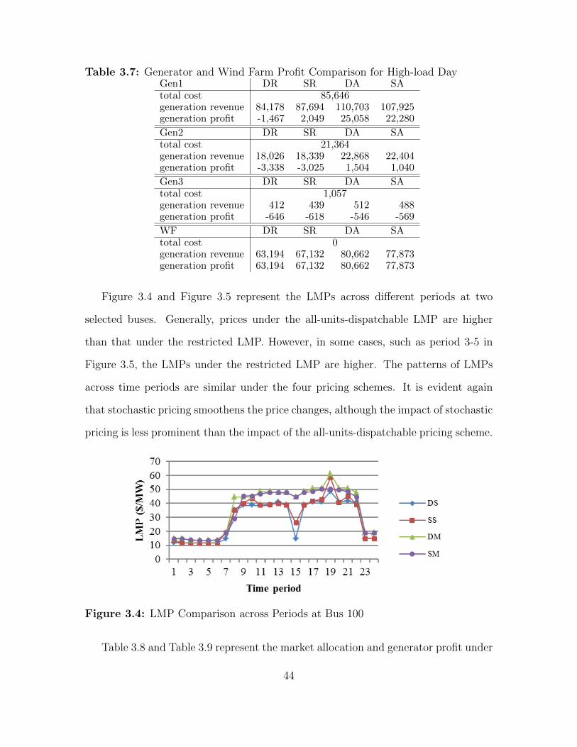
Table 3.7: Generator and Wind Farm Profit Comparison for High-load DayGen1 DR SR DA SAtotal cost 85,646generation revenue 84,178 87,694 110,703 107,925generation profit -1,467 2,049 25,058 22,280

Gen2 DR SR DA SAtotal cost 21,364generation revenue 18,026 18,339 22,868 22,404generation profit -3,338 -3,025 1,504 1,040

Gen3 DR SR DA SAtotal cost 1,057generation revenue 412 439 512 488generation profit -646 -618 -546 -569

WF DR SR DA SAtotal cost 0generation revenue 63,194 67,132 80,662 77,873generation profit 63,194 67,132 80,662 77,873

Figure 3.4 and Figure 3.5 represent the LMPs across different periods at two

selected buses. Generally, prices under the all-units-dispatchable LMP are higher

than that under the restricted LMP. However, in some cases, such as period 3-5 in

Figure 3.5, the LMPs under the restricted LMP are higher. The patterns of LMPs

across time periods are similar under the four pricing schemes. It is evident again

that stochastic pricing smoothens the price changes, although the impact of stochastic

pricing is less prominent than the impact of the all-units-dispatchable pricing scheme.

Figure 3.4: LMP Comparison across Periods at Bus 100

Table 3.8 and Table 3.9 represent the market allocation and generator profit under

44

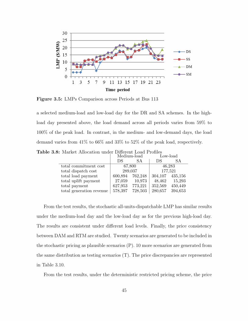
Figure 3.5: LMPs Comparison across Periods at Bus 113

a selected medium-load and low-load day for the DR and SA schemes. In the high-

load day presented above, the load demand across all periods varies from 59% to

100% of the peak load. In contrast, in the medium- and low-demand days, the load

demand varies from 41% to 66% and 33% to 52% of the peak load, respectively.

Table 3.8: Market Allocation under Different Load ProfilesMedium-load Low-loadDS SA DS SA

total commitment cost 67,800 46,283total dispatch cost 289,037 177,521total load payment 600,894 762,248 304,107 435,156total uplift payment 27,059 10,973 48,462 15,293total payment 627,953 773,221 352,569 450,449total generation revenue 578,397 728,503 280,657 394,653

From the test results, the stochastic all-units-dispatchable LMP has similar results

under the medium-load day and the low-load day as for the previous high-load day.

The results are consistent under different load levels. Finally, the price consistency

between DAM and RTM are studied. Twenty scenarios are generated to be included in

the stochastic pricing as plausible scenarios (P). 10 more scenarios are generated from

the same distribution as testing scenarios (T). The price discrepancies are represented

in Table 3.10.

From the test results, under the deterministic restricted pricing scheme, the price

45

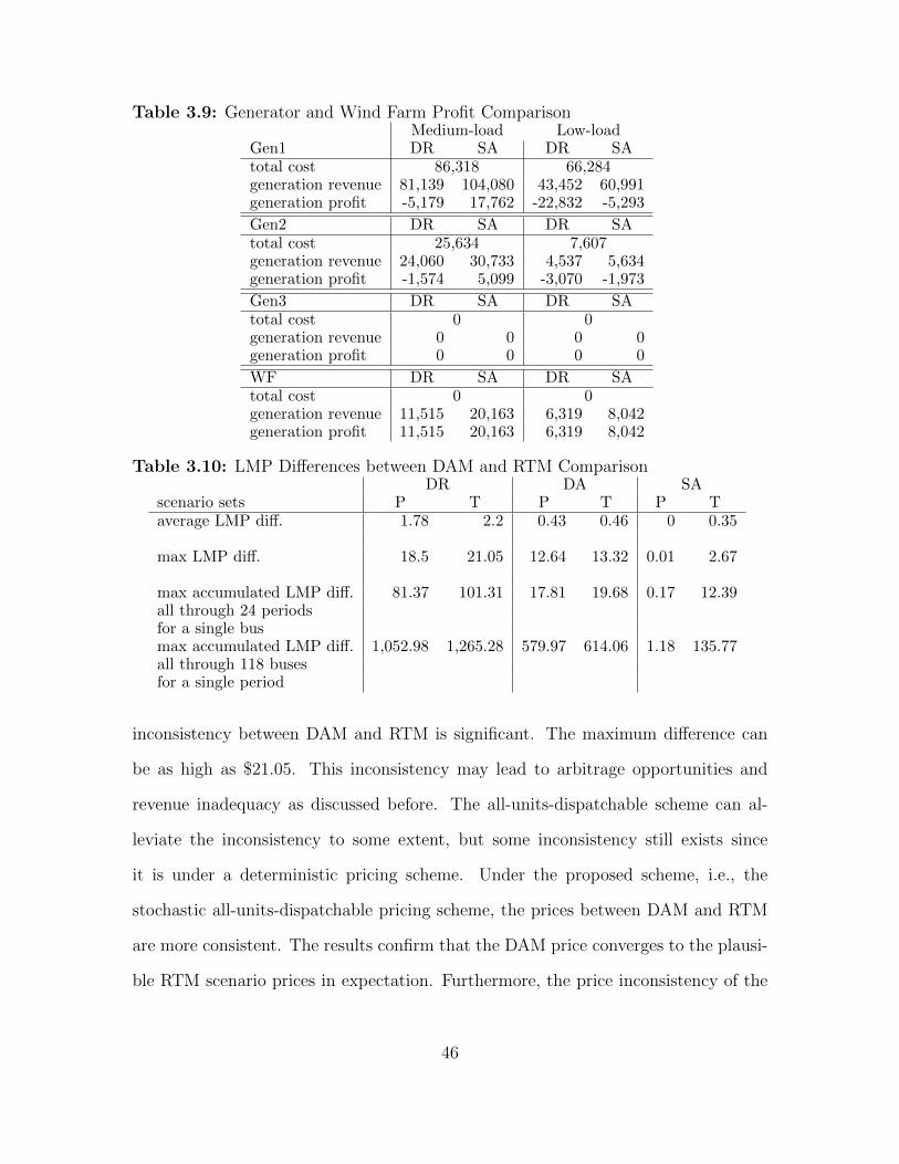
Table 3.9: Generator and Wind Farm Profit ComparisonMedium-load Low-load

Gen1 DR SA DR SAtotal cost 86,318 66,284generation revenue 81,139 104,080 43,452 60,991generation profit -5,179 17,762 -22,832 -5,293

Gen2 DR SA DR SAtotal cost 25,634 7,607generation revenue 24,060 30,733 4,537 5,634generation profit -1,574 5,099 -3,070 -1,973

Gen3 DR SA DR SAtotal cost 0 0generation revenue 0 0 0 0generation profit 0 0 0 0

WF DR SA DR SAtotal cost 0 0generation revenue 11,515 20,163 6,319 8,042generation profit 11,515 20,163 6,319 8,042

Table 3.10: LMP Differences between DAM and RTM ComparisonDR DA SA

scenario sets P T P T P Taverage LMP diff. 1.78 2.2 0.43 0.46 0 0.35

max LMP diff. 18.5 21.05 12.64 13.32 0.01 2.67

max accumulated LMP diff. 81.37 101.31 17.81 19.68 0.17 12.39all through 24 periodsfor a single busmax accumulated LMP diff. 1,052.98 1,265.28 579.97 614.06 1.18 135.77all through 118 busesfor a single period

inconsistency between DAM and RTM is significant. The maximum difference can

be as high as $21.05. This inconsistency may lead to arbitrage opportunities and

revenue inadequacy as discussed before. The all-units-dispatchable scheme can al-

leviate the inconsistency to some extent, but some inconsistency still exists since

it is under a deterministic pricing scheme. Under the proposed scheme, i.e., the

stochastic all-units-dispatchable pricing scheme, the prices between DAM and RTM

are more consistent. The results confirm that the DAM price converges to the plausi-

ble RTM scenario prices in expectation. Furthermore, the price inconsistency of the

46

proposed pricing scheme for the testing scenarios is much smaller than for the other

two schemes.

3.4 Conclusions

The proposed stochastic dispatchable pricing scheme addresses both the non-

convexity and uncertainty issues in the day-ahead energy market. Electricity markets

are non-convex so that a perfect equilibrium market clearing price may not exist, but

the proposed pricing scheme amortizes commitment costs into generation variable

costs and relaxes all units to be dispatchable to set energy prices. The scheme gives a

monotonically non-decreasing marginal cost function with respect to total loads. Test

results show that uplift payments are reduced and the generators with low generation

variable costs obtain higher profits in the energy market under the proposed pricing

scheme. The price changes are further smoothened by incorporating a set of scenarios

and using a stochastic pricing framework to set DAM energy prices. Test results show

that price jumps are alleviated by introducing the stochastic pricing framework, but

the impacts are less prominent than the ones from the dispatchable scheme.

In general, the test results indicate that the proposed stochastic all-units-dispatchable

LMP scheme gives better pricing signals and reduced need for uplift payments com-

pared to the currently utilized restricted LMP. In the short-term, the proposed pricing

scheme will result in a transfer of surplus from consumers to producers in the energy

market due to higher prices. However, other transfers could adjust for this in aggre-

gate, e.g., through reduced need for capacity payments, without changing incentives

on the margin. The proposed stochastic pricing scheme also leads to more price con-

sistency between day-ahead and real-time markets, leading to improved incentives for

market participants, which may change their bidding behavior accordingly. In the

long run, the proposed pricing scheme may incentivize investments in technologies

47

with low-variable-cost generation, such as renewable energy, potentially leading to

higher social welfare. Future studies are needed to analyze the long-term implica-

tions and confirm this hypothesis. The impact of the proposed pricing scheme on

other markets such as the financial transmission rights market, the ancillary services

market, and the capacity market, are also left for future study.

48

Chapter 4

ARBITRAGE IN ENERGY MARKETS

4.1 Introduction

The electric power industry is an $840-billion industry in the U.S., which repre-

sents approximately 3 percent of real gross domestic product (Edison Electric Insti-

tute, 2013). Each year, electric utilities spend roughly 200 billion in their planning

and operations (Energy Information Administration, 2015). Unlike other commodi-

ties in markets, the demand of electric power is considered to be very close to perfectly

inelastic. Thus, the imbalance between supply and demand can cause severe issues

in power grids. Consequently, one of the most challenging problems in electric power

scheduling is the uncertainty. Generally, the uncertainties in electric power schedul-

ing can be categorized as discrete or continuous uncertainties. Discrete uncertainties

include the failure of a single generator or transmission line, also known as an N-1

contingency. Continuous uncertainties include the loads and renewable energy vari-

ations with respect to their predicted levels. Nowadays, more and more renewable

energy resources (mainly wind and solar farms) are being built to provide electric

power in order to lower generation costs and reduce environmental pollutions. Ac-

cording to the California Renewables Portfolio Standard (RPS) (California Public

Utilities Commission, 2015), eligible renewable energy resources in California will be

increased to % of total production by 2020, compared to the current 12% nationwide

renewable generation (Energy Information Administration, 2014).

While it brings many benefits both economically and environmentally, on the

other hand, the high penetration of intermittent renewables also complicates power

49

scheduling due to the uncertain nature of the renewable energy. With high renew-

able penetration in the power grid, electric energy storage (EES) is one way to assist

handling resource uncertainties (Sandia National Laboratories, 2013). The technolo-

gies of EES are widely discussed in literature (Sandia National Laboratories, 2013;

Beaudin et al., 2010; Swierczynski et al., 2010; Ruggiero and Heydt, 2013; Divya and

Østergaard, 2009; Wade et al., 2010). Pumped hydro storage (PHS), which pumps

and discharges water from different reservoirs to store and release electric energy, is

the most common and well-developed form of energy storage, representing approxi-

mately 3% of the world’s total installed power capacity, and 97% of the total storage

capacity (Beaudin et al., 2010). PHS is popular for its high round-trip charging effi-

ciency (65-85%), large power capacity (100-1000MW), large energy storage capacity

(12+ hours), long life (30-60 years), and low cycle cost; however, PHS is limited by

its high capital cost ($100 million - $3 billion), long project lead time (typically ten

years), environmental damages, and its unique geographical requirements (Beaudin

et al., 2010). Compressed air energy storage (CAES) is another currently suitable

technique other than PHS for large-scale EES. CAES compresses the air into large

storage reservoirs using cheaper off-peak electric power instead of expensive gas and

releases the air for the conventional gas turbine cycles during peak hours (Ruggiero

and Heydt, 2013). CAES shares many of the same attractive characteristics of PHS,

but has significantly lower capital cost and little environmental impact since the stor-

age is underground (Beaudin et al., 2010). Nevertheless, there are only two CAES

plants in the world, one in Germany built in 1978 and another in Alabama, U.S. built

in 1991 (Beaudin et al., 2010). A variety of batteries have also been developed for

EES including, but not limited to, lead-acid, nickel-cadmium, sodium-sulfur, lithium-

ion, sodium-nickel-chloride, zinc-bromine, vanadium-redox and polysulphide-bromide

batteries. Their characteristics are discussed in (Sandia National Laboratories, 2013;

50

Beaudin et al., 2010; Swierczynski et al., 2010; Ruggiero and Heydt, 2013; Divya

and Østergaard, 2009; Wade et al., 2010). Other technologies such as flywheels, ca-

pacitors and super-capacitors, hydrogen storage, superconducting magnetic energy

storage (SMES), and solar thermal energy storage have been developed or are under

development for various EES purposes (Sandia National Laboratories, 2013; Beaudin

et al., 2010; Swierczynski et al., 2010; Ruggiero and Heydt, 2013; Divya and Øster-

gaard, 2009; Wade et al., 2010).

As for arbitrage in electric power market, EES owners buy the energy during the

off-peak hours with low price and sell it in the peak hours with higher price in order

to make profits. Therefore, EES devices should have higher power capacity (20+MW

is desired) and higher energy storage capacity (4+ hours is desired). Currently, only

PHS, CAES, sodium-sulfur battery and lead-acid battery are suitable for arbitrage

in the markets.

In addition to responding to the intermittent renewable resources, introducing

EES to the power grid can benefit the system in several ways. Large-scale EES was

initially studied focusing on the peak load shaving effects. Social welfare can be

improved by moving the peak load to the off-peak periods by utilizing EES and, as a

result, the electricity price variability is typically reduced. Moreover, introducing EES

can defer facility investments (Sioshansi et al., 2009). While such benefits exist, such

welfare benefits may not be captured by the private investor of EES. As the private

investors, they gain profits relying on pricing arbitrage. Since large-scale EES will

smooth load and reduce price variance in different periods, the diminished value of

arbitrage can be expected, which contradicts the investors’ motivation of investing in

EES facilities. Therefore, despite the benefits that EES will bring to power systems,

the current market settings give limited incentives for the private investors to build

EES facilities. The ownerships of EES facilities, contracts for EES in the markets,

51

and government subsidies have been discussed but not yet implemented (Sioshansi

et al., 2009). An enhanced market design that is conducive to EES is left for future

study.

The remainder of this chapter is organized as follows: Section 4.2 gives the math-

ematical formulations. Section 4.3 discusses three charging policies to hedge uncer-

tainty for the arbitrager. Section 4.4 carries out a case study on the IEEE 118-bus

system and shows the computational results. Finally, Section 4.5 draws the conclu-

sions.

4.2 Mathematical Formulations

In the models in this chapter, a power transfer distribution factor (PTDF) based

direct current optimal power flow model (DCOPF) is adopted, which is a linear

approximation of real power flow with a set of simplifying assumptions (Wood and

Wollenberg, 1996; Stott et al., 2009).

4.2.1 Location Selection Model

Since most energy markets in the U.S. now have a nodal market settlement struc-

ture, the location of EES will play an important role. The EES location selections

depend on whether the owner of EES is a vertically-integrated utility or a for-profit

private entity. For vertically-integrated utilities, the objective should be to minimize

the total costs. Then the EESs are preferred at the locations where the whole system

will benefit. On the other hand, in regards to for-profit private entities, the EES

facilities are preferred at the locations where the owner can maximize the individual

profits by arbitrage. The following model gives the optimal locations for minimiz-

ing total costs, the perspective of the vertically-integrated utility. Generally, these

locations are not the optimal locations from a for-profit EES owner’s point of view.

52

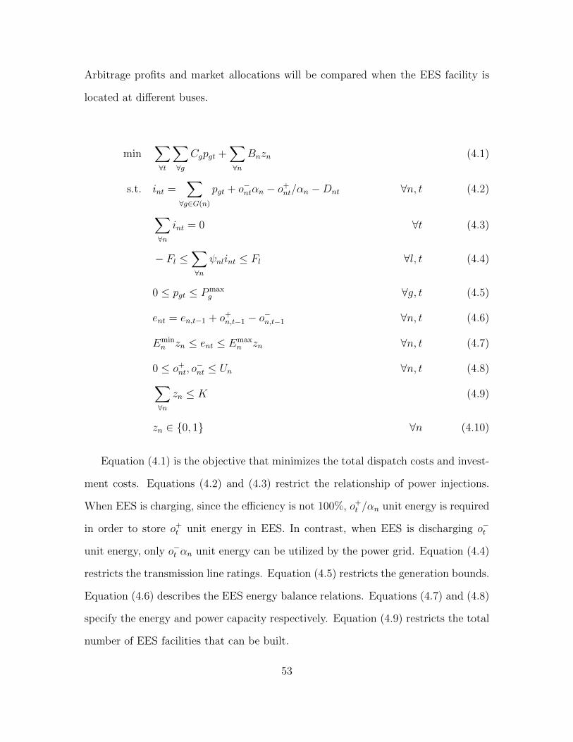
Arbitrage profits and market allocations will be compared when the EES facility is

located at different buses.

min∑∀t

∑∀g

Cgpgt +∑∀n

Bnzn (4.1)

s.t. int =∑∀g∈G(n)

pgt + o−ntαn − o+nt/αn −Dnt ∀n, t (4.2)

∑∀n

int = 0 ∀t (4.3)

− Fl ≤∑∀n

ψnlint ≤ Fl ∀l, t (4.4)

0 ≤ pgt ≤ Pmaxg ∀g, t (4.5)

ent = en,t−1 + o+n,t−1 − o−n,t−1 ∀n, t (4.6)

Eminn zn ≤ ent ≤ Emax

n zn ∀n, t (4.7)

0 ≤ o+nt, o−nt ≤ Un ∀n, t (4.8)∑

∀n

zn ≤ K (4.9)

zn ∈ {0, 1} ∀n (4.10)

Equation (4.1) is the objective that minimizes the total dispatch costs and invest-

ment costs. Equations (4.2) and (4.3) restrict the relationship of power injections.

When EES is charging, since the efficiency is not 100%, o+t /αn unit energy is required

in order to store o+t unit energy in EES. In contrast, when EES is discharging o−t

unit energy, only o−t αn unit energy can be utilized by the power grid. Equation (4.4)

restricts the transmission line ratings. Equation (4.5) restricts the generation bounds.

Equation (4.6) describes the EES energy balance relations. Equations (4.7) and (4.8)

specify the energy and power capacity respectively. Equation (4.9) restricts the total

number of EES facilities that can be built.

53

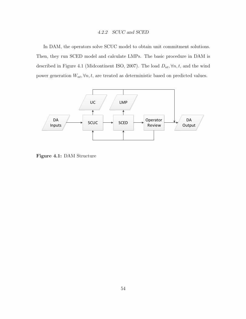
4.2.2 SCUC and SCED

In DAM, the operators solve SCUC model to obtain unit commitment solutions.

Then, they run SCED model and calculate LMPs. The basic procedure in DAM is

described in Figure 4.1 (Midcontinent ISO, 2007). The load Dnt,∀n, t, and the wind

power generation Wnt,∀n, t, are treated as deterministic based on predicted values.

DA Inputs

SCUC SCEDOperator Review

UC LMP

DA Output

Figure 4.1: DAM Structure

54

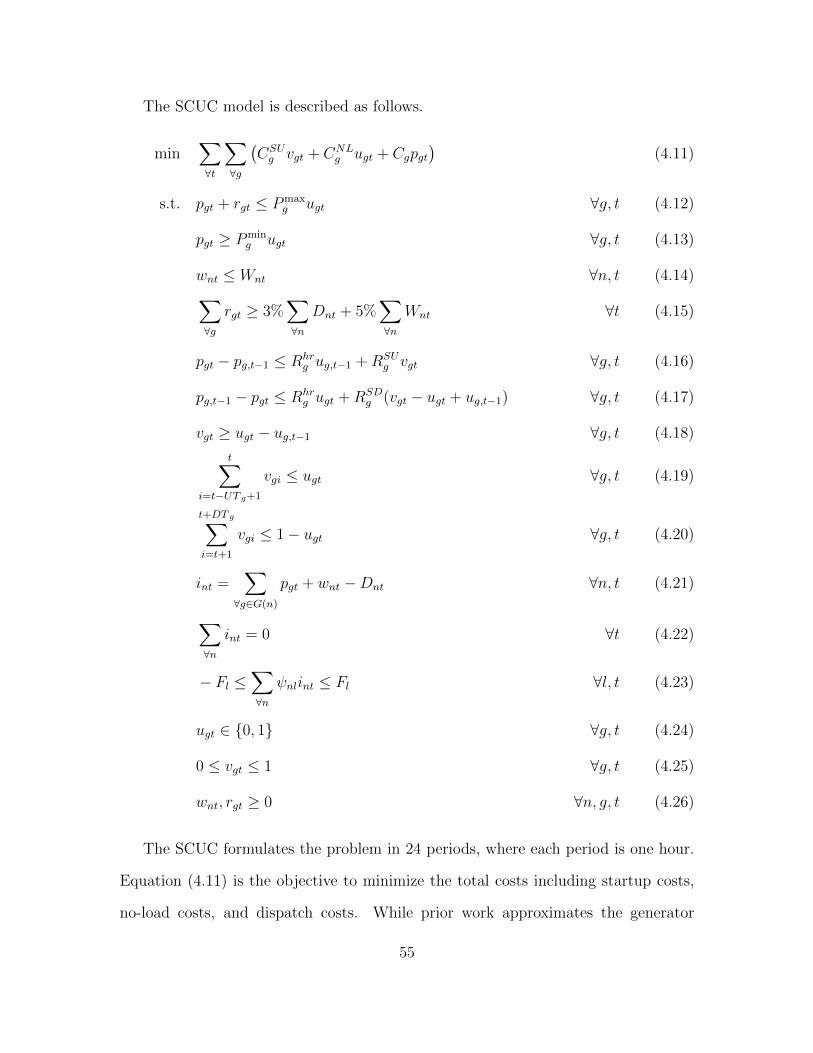
The SCUC model is described as follows.

min∑∀t

∑∀g

(CSUg vgt + CNL

g ugt + Cgpgt)

(4.11)

s.t. pgt + rgt ≤ Pmaxg ugt ∀g, t (4.12)

pgt ≥ Pming ugt ∀g, t (4.13)

wnt ≤ Wnt ∀n, t (4.14)∑∀g

rgt ≥ 3%∑∀n

Dnt + 5%∑∀n

Wnt ∀t (4.15)

pgt − pg,t−1 ≤ Rhrg ug,t−1 +RSU

g vgt ∀g, t (4.16)

pg,t−1 − pgt ≤ Rhrg ugt +RSD

g (vgt − ugt + ug,t−1) ∀g, t (4.17)

vgt ≥ ugt − ug,t−1 ∀g, t (4.18)

t∑i=t−UT g+1

vgi ≤ ugt ∀g, t (4.19)

t+DT g∑i=t+1

vgi ≤ 1− ugt ∀g, t (4.20)

int =∑∀g∈G(n)

pgt + wnt −Dnt ∀n, t (4.21)

∑∀n

int = 0 ∀t (4.22)

− Fl ≤∑∀n

ψnlint ≤ Fl ∀l, t (4.23)

ugt ∈ {0, 1} ∀g, t (4.24)

0 ≤ vgt ≤ 1 ∀g, t (4.25)

wnt, rgt ≥ 0 ∀n, g, t (4.26)

The SCUC formulates the problem in 24 periods, where each period is one hour.

Equation (4.11) is the objective to minimize the total costs including startup costs,

no-load costs, and dispatch costs. While prior work approximates the generator

55

cost curve as a quadratic function, the presented model assumes a piecewise linear

formulation, which is consistent with existing market structures. Since the market

model is non-convex, uplift payments may be required to ensure a non-confiscatory

market. Equations (4.12) and (4.13) restrict the generation upper bound and lower

bound. When the generator is not committed, i.e., ugt = 0, the generation (pgt

and rgt) is forced to be zero. Equation (4.14) restricts the wind power injection to

be less than the maximum power that the wind farm can provide. Although the

marginal cost of the wind power is zero, it is not always the case that dispatching

all available wind power is beneficial. Due to transmission congestion and due to

ramping limitations, it is at times cheaper to spill wind as opposed to displacing

fossil fuel based production. Equation (4.15) specifies the system reserves in order to

handle uncertainties. The ad-hoc 3+5 requirement rule, which requires the reserves

to be more than 3% of the total predicted load and 5% of the total predicted wind

power, is adopted (Papavasiliou et al., 2011). Equations (4.16) and (4.17) restrict

the hourly ramping up and ramping down constraints. Equation (4.18) specifies the

relation between the unit commitment status and the startup status. Equations (4.19)

and (4.20) impose the minimum up and down time constraints, which states that if a

generator is turned on, it cannot be turned down in the next UTg hours; similarly, if

it is turned off, it cannot be turned on in the next DTg hours. Equations (4.21) and

(4.22) define the bus injection. Equation (4.23) imposes the transmission line rating.

The generation shift factors are results from Kirchhoff’s laws. Equations (4.24)-(4.26)

specify the variable restrictions. The startup variable is relaxed to be continuous but

is guaranteed to be either 0 or 1, since (4.18)-(4.20) form the facet-defining constraint

of u, v projection Rajan and Takriti (2005).

56

The SCED is described as follows.

min∑∀t

∑∀g

Cgpgt (4.27)

s.t. Pming ugt ≤ pgt ≤ Pmax

g ugt ∀g, t (4.28)

0 ≤ wnt ≤ Wnt ∀n, t (4.29)

int =∑∀g∈G(n)

pgt + wnt −Dnt ∀n, t (4.30)

∑∀n

int = 0 ∀t (4.31)

− Fl ≤∑∀n

ψnlint ≤ Fl ∀l, t (4.32)

pgt − pg,t−1 ≤ Rhrg ug,t−1 +RSU

g vgt ∀g, t (4.33)

pg,t−1 − pgt ≤ Rhrg ugt +RSD

g (vgt − ugt + ug,t−1) ∀g, t (4.34)

In the SCED with network constraints model, the objective (4.27) only minimizes

the dispatching costs. Equations (4.28)-(4.34) are the same as (4.12)-(4.14), (4.21)-

(4.23), (4.16)-(4.17), with the exceptions: one, for simplicity, the real-time market

is modeled as an energy-only market; two, the unit commitment variables and the

startup variables are fixed. The LMPs are the dual variables of (4.30).

4.2.3 Arbitrage Model

In the following arbitrage models, it is assumed that the decision maker is a private

investor who maximizes their arbitrage profits. EES is located at a single location k.

Prior work frequently assumes that the arbitragers are price-takers, i.e., the par-

ticipation of EES has little impact on the real-time LMPs and charging or discharging

decisions are made based on the predicted LMP (Sioshansi et al., 2009; Walawalkar

et al., 2007; Connolly et al., 2011). Due to the generally small size of EES, this

assumption is valid.

57

The EES owner runs the following model to maximize profits.

max∑∀t

λkt(o−t αk − o+t /αk) (4.35)

s.t. et = et−1 + o+t − o−t ∀t (4.36)

Emink ≤ et ≤ Emax

k ∀t (4.37)

0 ≤ o+t , o−t ≤ Uk ∀t (4.38)

Equation (4.35) maximizes the profit with the predicted LMPs, λkt, as a fixed

constant. Equation (4.36) restricts the energy balance constraint and (4.37)-(4.38)

specify the energy and power capacities respectively.

The price-taker assumption may not be true if the charging and discharging have

a strong influence on its LMP. In this chapter, the focus is on how the LMP changes

induced by the charging or discharging may affect the optimal schedule for EES.

Actually, the LMPs λkt become a function of charging or discharging decisions o+t , o−t ,

i.e., the λkt will change as the o+t , o−t changes. Therefore, EES owner needs to consider

this relation while making their charging decision to maximize profits. The following

arbitrage model solves the optimization problem and returns the optimal charging

and discharging decisions. The model is described in six parts: objective, primal

constraints, dual constraints, strong duality constraint, linearizing constraints, and

EES constraints. The model is described as follows.

Objective

max Qk

∑∀t

∑∀j

(η−jtαk − η+jt/αk) (4.39)

Equation (4.39) is the objective to maximize the investor’s profits. In (4.35), when

λkt is the function of o+t , o−t , λkt also becomes the variable in the optimization problem.

58

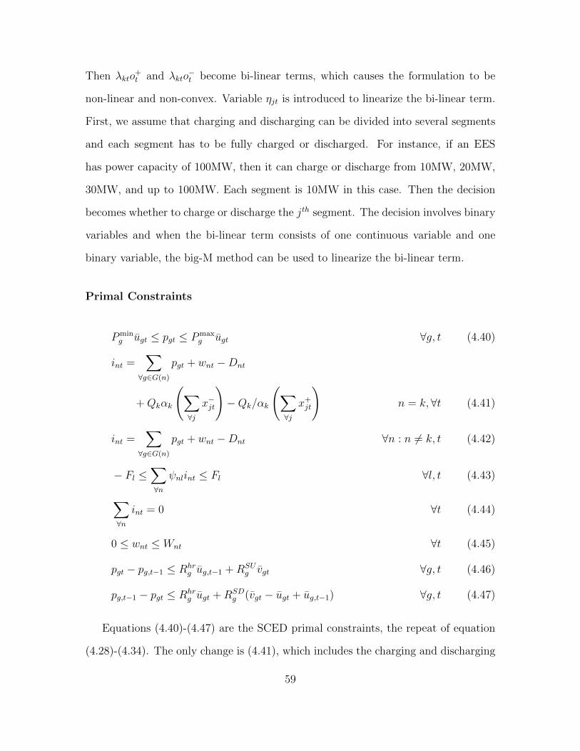
Then λkto+t and λkto

−t become bi-linear terms, which causes the formulation to be

non-linear and non-convex. Variable ηjt is introduced to linearize the bi-linear term.

First, we assume that charging and discharging can be divided into several segments

and each segment has to be fully charged or discharged. For instance, if an EES

has power capacity of 100MW, then it can charge or discharge from 10MW, 20MW,

30MW, and up to 100MW. Each segment is 10MW in this case. Then the decision

becomes whether to charge or discharge the jth segment. The decision involves binary

variables and when the bi-linear term consists of one continuous variable and one

binary variable, the big-M method can be used to linearize the bi-linear term.

Primal Constraints

Pming ugt ≤ pgt ≤ Pmax

g ugt ∀g, t (4.40)

int =∑∀g∈G(n)

pgt + wnt −Dnt

+Qkαk

(∑∀j

x−jt

)−Qk/αk

(∑∀j

x+jt

)n = k,∀t (4.41)

int =∑∀g∈G(n)

pgt + wnt −Dnt ∀n : n 6= k, t (4.42)

− Fl ≤∑∀n

ψnlint ≤ Fl ∀l, t (4.43)

∑∀n

int = 0 ∀t (4.44)

0 ≤ wnt ≤ Wnt ∀t (4.45)

pgt − pg,t−1 ≤ Rhrg ug,t−1 +RSU

g vgt ∀g, t (4.46)

pg,t−1 − pgt ≤ Rhrg ugt +RSD

g (vgt − ugt + ug,t−1) ∀g, t (4.47)

Equations (4.40)-(4.47) are the SCED primal constraints, the repeat of equation

(4.28)-(4.34). The only change is (4.41), which includes the charging and discharging

59

events at bus k.

Dual Constraints

− φ+gt + φ−gt + λg(n),t − ρ+gt + ρ+g,t+1 − ρ−g,t+1 + ρ−gt = Cg ∀g, t (4.48)

λnt − ωnt ≤ 0 ∀n, t (4.49)

− λnt −∑∀l

ψnl(µ+lt − µ

−lt ) + τt = 0 ∀n, t (4.50)

φ+gt, φ

−gt, ρ

+gt, ρ

−gt, µ

+lt , µ

−lt , ωnt ≥ 0 ∀g, l, n, t (4.51)

Equations (4.48)-(4.51) are the SCED dual constraints. When taking the dual, the

charging and discharging decisions are treated as known constants. The variables are

generation level pgt, dispatched wind power wnt, and bus injection int. Each constraint

of (4.48)-(4.50) is one-to-one corresponding to the three variables and equation (4.51)

specifies the sign restriction of each variable.

Strong Duality Constraints

∑∀t

∑∀g

Cgpgt =∑∀t

∑∀n

(Dntλnt +Wntωnt)

−∑∀t

∑∀g

ugt(Pmaxg φ+

gt − Pming φ−gt)

−Qk

∑∀t

∑∀j

(η−jtαk − η+jt/αk)

−∑∀t

∑∀l

Fl(µ+lt + µ−lt )

−∑∀t

∑∀g

(Rhrg ug,t−1 +RSU

g vgt)ρ+gt

−∑∀t

∑∀g

[Rhrg ugt +RSD

g (vgt − ugt + ug,t−1)]ρ−gt (4.52)

60

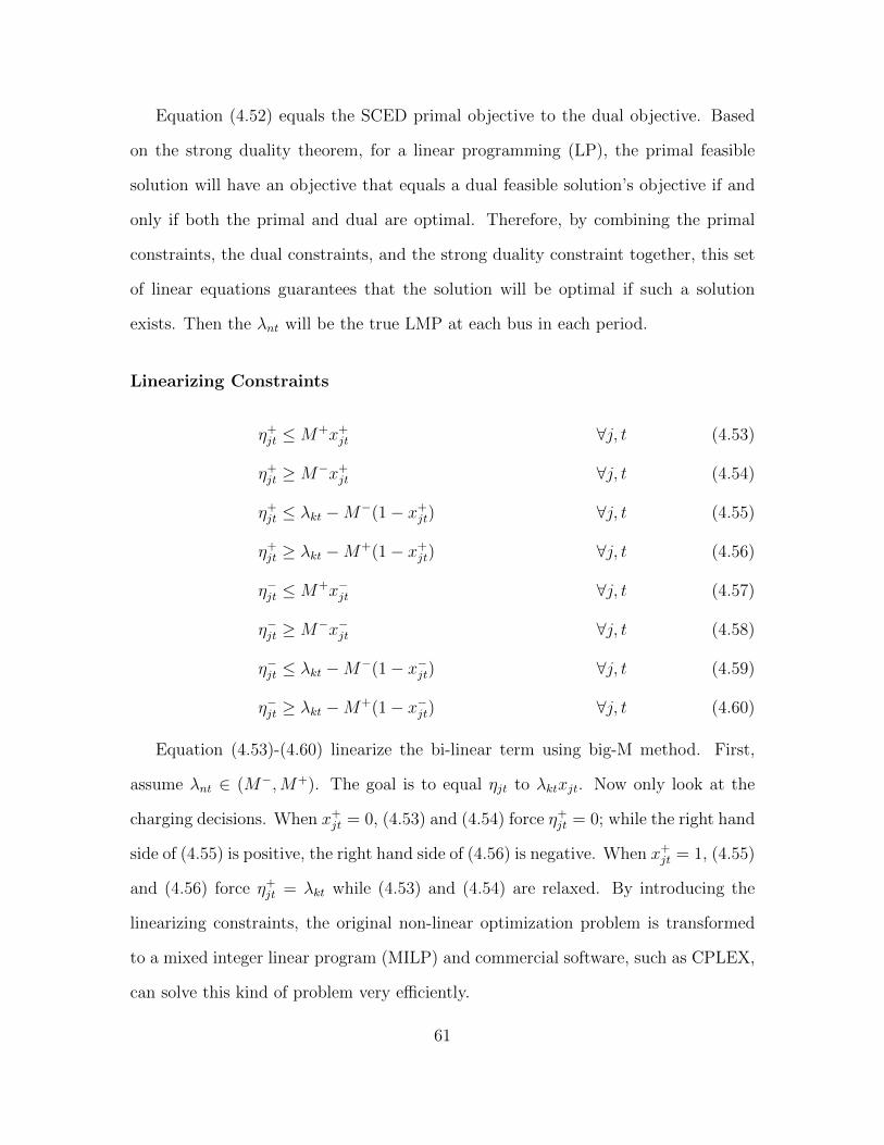
Equation (4.52) equals the SCED primal objective to the dual objective. Based

on the strong duality theorem, for a linear programming (LP), the primal feasible

solution will have an objective that equals a dual feasible solution’s objective if and

only if both the primal and dual are optimal. Therefore, by combining the primal

constraints, the dual constraints, and the strong duality constraint together, this set

of linear equations guarantees that the solution will be optimal if such a solution

exists. Then the λnt will be the true LMP at each bus in each period.

Linearizing Constraints

η+jt ≤M+x+jt ∀j, t (4.53)

η+jt ≥M−x+jt ∀j, t (4.54)

η+jt ≤ λkt −M−(1− x+jt) ∀j, t (4.55)

η+jt ≥ λkt −M+(1− x+jt) ∀j, t (4.56)

η−jt ≤M+x−jt ∀j, t (4.57)

η−jt ≥M−x−jt ∀j, t (4.58)

η−jt ≤ λkt −M−(1− x−jt) ∀j, t (4.59)

η−jt ≥ λkt −M+(1− x−jt) ∀j, t (4.60)

Equation (4.53)-(4.60) linearize the bi-linear term using big-M method. First,

assume λnt ∈ (M−,M+). The goal is to equal ηjt to λktxjt. Now only look at the

charging decisions. When x+jt = 0, (4.53) and (4.54) force η+jt = 0; while the right hand

side of (4.55) is positive, the right hand side of (4.56) is negative. When x+jt = 1, (4.55)

and (4.56) force η+jt = λkt while (4.53) and (4.54) are relaxed. By introducing the

linearizing constraints, the original non-linear optimization problem is transformed

to a mixed integer linear program (MILP) and commercial software, such as CPLEX,

can solve this kind of problem very efficiently.

61

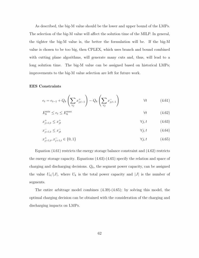
As described, the big-M value should be the lower and upper bound of the LMPs.

The selection of the big-M value will affect the solution time of the MILP. In general,

the tighter the big-M value is, the better the formulation will be. If the big-M

value is chosen to be too big, then CPLEX, which uses branch and bound combined

with cutting plane algorithms, will generate many cuts and, thus, will lead to a

long solution time. The big-M value can be assigned based on historical LMPs;

improvements to the big-M value selection are left for future work.

EES Constraints

et = et−1 +Qk

(∑∀j

x+j,t−1

)−Qk

(∑∀j

x−j,t−1

)∀t (4.61)

Emink ≤ et ≤ Emax

k ∀t (4.62)

x+j+1,t ≤ x+jt ∀j, t (4.63)

x−j+1,t ≤ x−jt ∀j, t (4.64)

x+j+1,t, x−j+1,t ∈ {0, 1} ∀j, t (4.65)

Equation (4.61) restricts the energy storage balance constraint and (4.62) restricts

the energy storage capacity. Equations (4.63)-(4.65) specify the relation and space of

charging and discharging decisions. Qk, the segment power capacity, can be assigned

the value Uk/|J |, where Uk is the total power capacity and |J | is the number of

segments.

The entire arbitrage model combines (4.39)-(4.65); by solving this model, the

optimal charging decision can be obtained with the consideration of the charging and

discharging impacts on LMPs.

62

4.3 Electric Energy Storage Charging Policies

In the previous section, all models are deterministic models, i.e., the loads and

the wind power are fixed at their predicted values. However, due to uncertainty, real-

time LMPs will deviate away from their predicted values, which leads to sub-optimal

arbitrage decisions, which can also cause negative profits. Three charging policies are

discussed in this section. SCUC is first solved to obtain the unit commitment solution

for the next 24 hours. Then the arbitrage model is solved under different polices to

obtain the charging and discharging solutions. Finally, in the real-time market, the

EES owner participates in the market based on the obtained charging schedule. The

procedure is described in Figure 4.2.

Figure 4.2: EES Charging/Discharging Decision Procedure

4.3.1 Forecasting-belief Policy

In this policy, the EES owner makes the decision based on the day-ahead forecast-

ing loads and wind power assuming that they are the true value in the real-time. The

arbitrage model is run with the predicted loads and wind power. Once the EES owner

obtains the charging solutions, they stick to the charging and discharging schedule in

63

the real-time market for the next 24 hours.

4.3.2 Robust Policy

In this robust policy, the EES owner first simulates several scenarios using Monte

Carlo simulations. Then, they run the arbitrage model to estimate the best charging

decision, the LMPs, and the total profits for each simulated scenario. Finally, they

make the final charging decision based on these generated scenario solutions. Specifi-

cally, this policy calculates the lower and upper bound for the LMPs. Then the EES

owner uses the maximum LMP when buying energy and the minimum LMP when

selling the energy. In such manner, they hedge the risk of LMP variation that the

wind and load uncertainty may bring to the power grid.

4.3.3 Dynamic Policy

The wind power is highly related to the wind speed. In practice, the wind speed

is usually predicted first and the wind power is calculated with some static non-

linear function with respect to the wind speed (Papavasiliou and Oren, 2013). A

better wind speed prediction can be obtained when the predicted period is close to

the current period. In this dynamic policy, the EES owner updates their charging

decision periodically. Standing at the current hour, the EES owner can have a better

wind speed prediction of the following few hours. At each period, they run the

arbitrage model for the next 24 hours and they keep adjusting the charging decision

dynamically. This policy takes the advantage of the better prediction of the wind

power and more accurate real-time LMPs. Figure 4.3 describes the procedure of the

dynamic policy.

64

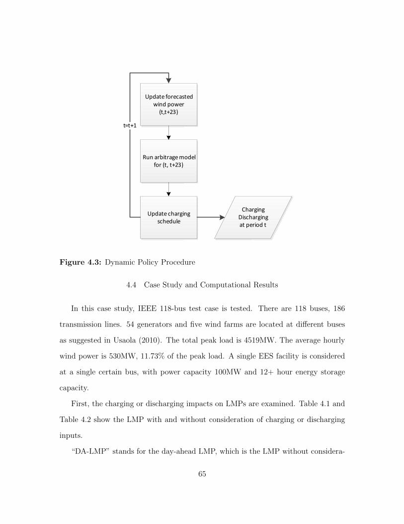
Update forecasted wind power

(t,t+23)

Run arbitrage model for (t, t+23)

Update charging schedule

Charging Discharging at period t

t=t+1

Figure 4.3: Dynamic Policy Procedure

4.4 Case Study and Computational Results

In this case study, IEEE 118-bus test case is tested. There are 118 buses, 186

transmission lines. 54 generators and five wind farms are located at different buses

as suggested in Usaola (2010). The total peak load is 4519MW. The average hourly

wind power is 530MW, 11.73% of the peak load. A single EES facility is considered

at a single certain bus, with power capacity 100MW and 12+ hour energy storage

capacity.

First, the charging or discharging impacts on LMPs are examined. Table 4.1 and

Table 4.2 show the LMP with and without consideration of charging or discharging

inputs.

“DA-LMP” stands for the day-ahead LMP, which is the LMP without considera-

65

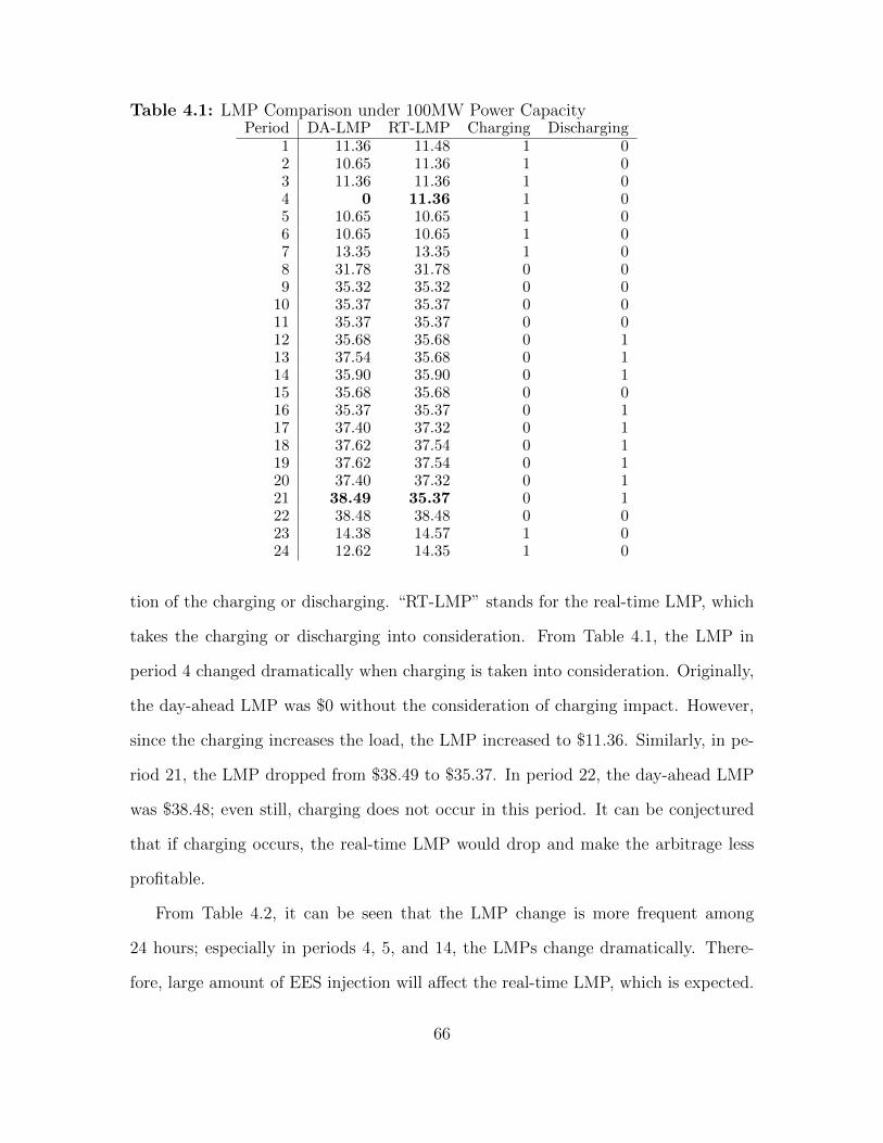
Table 4.1: LMP Comparison under 100MW Power CapacityPeriod DA-LMP RT-LMP Charging Discharging

1 11.36 11.48 1 02 10.65 11.36 1 03 11.36 11.36 1 04 0 11.36 1 05 10.65 10.65 1 06 10.65 10.65 1 07 13.35 13.35 1 08 31.78 31.78 0 09 35.32 35.32 0 0

10 35.37 35.37 0 011 35.37 35.37 0 012 35.68 35.68 0 113 37.54 35.68 0 114 35.90 35.90 0 115 35.68 35.68 0 016 35.37 35.37 0 117 37.40 37.32 0 118 37.62 37.54 0 119 37.62 37.54 0 120 37.40 37.32 0 121 38.49 35.37 0 122 38.48 38.48 0 023 14.38 14.57 1 024 12.62 14.35 1 0

tion of the charging or discharging. “RT-LMP” stands for the real-time LMP, which

takes the charging or discharging into consideration. From Table 4.1, the LMP in

period 4 changed dramatically when charging is taken into consideration. Originally,

the day-ahead LMP was $0 without the consideration of charging impact. However,

since the charging increases the load, the LMP increased to $11.36. Similarly, in pe-

riod 21, the LMP dropped from $38.49 to $35.37. In period 22, the day-ahead LMP

was $38.48; even still, charging does not occur in this period. It can be conjectured

that if charging occurs, the real-time LMP would drop and make the arbitrage less

profitable.

From Table 4.2, it can be seen that the LMP change is more frequent among

24 hours; especially in periods 4, 5, and 14, the LMPs change dramatically. There-

fore, large amount of EES injection will affect the real-time LMP, which is expected.

66

Table 4.2: LMP Comparison under 150MW Power CapacityPeriod DA-LMP RT-LMP Charging Discharging

1 11.36 11.20 0 02 11.36 11.03 1 03 11.36 11.03 1 04 0 11.20 1 05 0 11.21 1 06 10.65 11.13 1 07 10.76 13.84 0 08 31.78 25.62 0 09 35.32 35.32 0 0

10 35.28 35.28 0 011 35.28 35.28 0 012 35.68 35.68 0 013 35.68 35.68 0 014 35.90 14.44 0 115 14.40 14.40 0 016 35.37 35.37 0 017 37.32 35.68 0 118 37.62 35.90 0 119 37.62 35.41 0 120 37.32 35.03 0 121 38.49 38.49 0 022 38.48 38.46 0 023 14.38 14.38 0 024 12.62 12.62 0 0

When the EES owner makes the arbitrage decision, this effect should be taken into

consideration.

Next, different locations of EES are examined for arbitrage. Moreover, the market

welfare allocations are listed for comparison. Table 4.3 shows the results.

As discussed in section 4.2.1, the locational model is run assuming the EES owner

is a vertically-integrated utility. Specifically, all 118 buses are examined for their

potential load-shifting savings. A couple of potential EES locations are compared.

Bus 67 gives the optimal location for load-shifting savings. Bus 24 gives the minimum

savings per MW. Bus 8 gives the minimum total savings. Bus 70 gives the maximum

total charged MW. Bus 60 is the wind farm location with maximum average wind

power. Bus 89 is the bus with maximum load. Buses 28, 79, and 117 are randomly

selected bus.

67

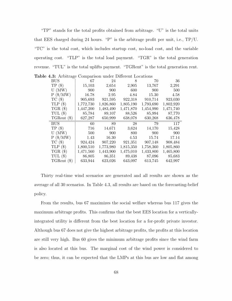
“TP” stands for the total profits obtained from arbitrage. “U” is the total units

that EES charged during 24 hours. “P” is the arbitrage profit per unit, i.e., TP/U.

“TC” is the total cost, which includes startup cost, no-load cost, and the variable

operating cost. “TLP” is the total load payment. “TGR” is the total generation

revenue. “TUL” is the total uplifts payment. “TGRent” is the total generation rent.

Table 4.3: Arbitrage Comparison under Different LocationsBUS 67 24 8 70 36TP ($) 15,103 2,654 2,905 13,767 2,291U (MW) 900 900 600 900 500P ($/MW) 16.78 2.95 4.84 15.30 4.58TC ($) 905,693 921,595 922,318 910,714 923,030TLP ($) 1,772,730 1,826,860 1,805,190 1,793,690 1,802,920TGR ($) 1,447,200 1,483,490 1,471,870 1,454,990 1,471,740TUL ($) 85,784 89,107 88,526 85,994 87,770TGRent ($) 627,287 650,999 638,078 630,268 636,478

BUS 60 89 28 79 117TP ($) 716 14,671 3,624 14,170 15,428U (MW) 500 900 800 900 900P ($/MW) 1.43 16.30 4.53 15.74 17.14TC ($) 924,424 907,220 921,351 907,148 908,484TLP ($) 1,800,510 1,773,980 1,815,350 1,758,360 1,805,860TGR ($) 1,471,560 1,443,900 1,475,010 1,433,800 1,465,800TUL ($) 86,805 86,351 89,438 87,096 85,683TGRent ($) 633,944 623,026 643,097 613,745 642,997

Thirty real-time wind scenarios are generated and all results are shown as the

average of all 30 scenarios. In Table 4.3, all results are based on the forecasting-belief

policy.

From the results, bus 67 maximizes the social welfare whereas bus 117 gives the

maximum arbitrage profits. This confirms that the best EES location for a vertically-

integrated utility is different from the best location for a for-profit private investor.

Although bus 67 does not give the highest arbitrage profits, the profits at this location

are still very high. Bus 60 gives the minimum arbitrage profits since the wind farm

is also located at this bus. The marginal cost of the wind power is considered to

be zero; thus, it can be expected that the LMPs at this bus are low and flat among

68

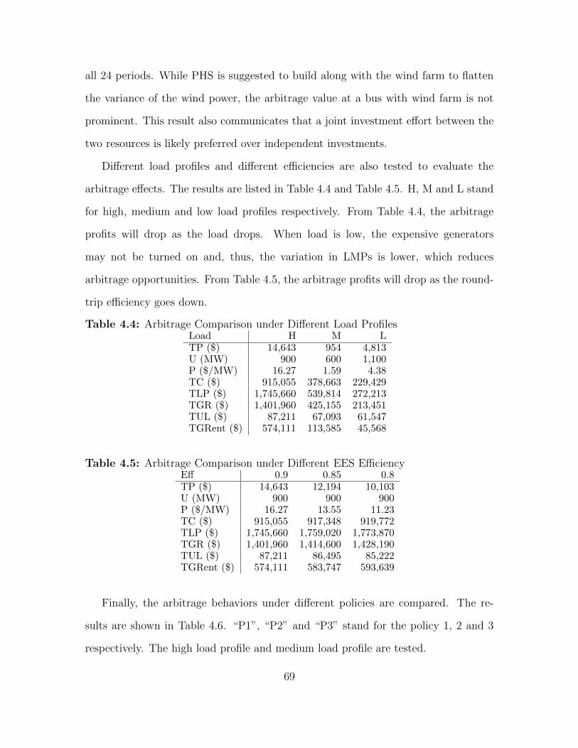
all 24 periods. While PHS is suggested to build along with the wind farm to flatten

the variance of the wind power, the arbitrage value at a bus with wind farm is not

prominent. This result also communicates that a joint investment effort between the

two resources is likely preferred over independent investments.

Different load profiles and different efficiencies are also tested to evaluate the

arbitrage effects. The results are listed in Table 4.4 and Table 4.5. H, M and L stand

for high, medium and low load profiles respectively. From Table 4.4, the arbitrage

profits will drop as the load drops. When load is low, the expensive generators

may not be turned on and, thus, the variation in LMPs is lower, which reduces

arbitrage opportunities. From Table 4.5, the arbitrage profits will drop as the round-

trip efficiency goes down.

Table 4.4: Arbitrage Comparison under Different Load ProfilesLoad H M LTP ($) 14,643 954 4,813U (MW) 900 600 1,100P ($/MW) 16.27 1.59 4.38TC ($) 915,055 378,663 229,429TLP ($) 1,745,660 539,814 272,213TGR ($) 1,401,960 425,155 213,451TUL ($) 87,211 67,093 61,547TGRent ($) 574,111 113,585 45,568

Table 4.5: Arbitrage Comparison under Different EES EfficiencyEff 0.9 0.85 0.8TP ($) 14,643 12,194 10,103U (MW) 900 900 900P ($/MW) 16.27 13.55 11.23TC ($) 915,055 917,348 919,772TLP ($) 1,745,660 1,759,020 1,773,870TGR ($) 1,401,960 1,414,600 1,428,190TUL ($) 87,211 86,495 85,222TGRent ($) 574,111 583,747 593,639

Finally, the arbitrage behaviors under different policies are compared. The re-

sults are shown in Table 4.6. “P1”, “P2” and “P3” stand for the policy 1, 2 and 3

respectively. The high load profile and medium load profile are tested.

69

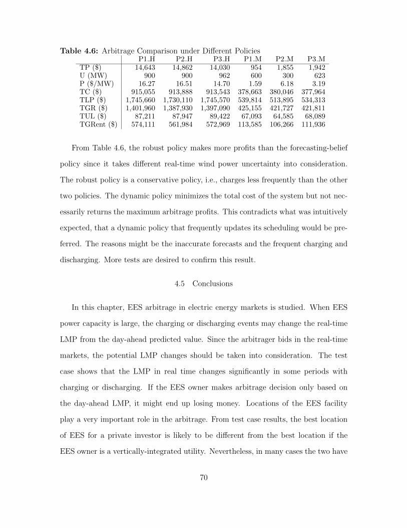
Table 4.6: Arbitrage Comparison under Different PoliciesP1 H P2 H P3 H P1 M P2 M P3 M

TP ($) 14,643 14,862 14,030 954 1,855 1,942U (MW) 900 900 962 600 300 623P ($/MW) 16.27 16.51 14.70 1.59 6.18 3.19TC ($) 915,055 913,888 913,543 378,663 380,046 377,964TLP ($) 1,745,660 1,730,110 1,745,570 539,814 513,895 534,313TGR ($) 1,401,960 1,387,930 1,397,090 425,155 421,727 421,811TUL ($) 87,211 87,947 89,422 67,093 64,585 68,089TGRent ($) 574,111 561,984 572,969 113,585 106,266 111,936

From Table 4.6, the robust policy makes more profits than the forecasting-belief

policy since it takes different real-time wind power uncertainty into consideration.

The robust policy is a conservative policy, i.e., charges less frequently than the other

two policies. The dynamic policy minimizes the total cost of the system but not nec-

essarily returns the maximum arbitrage profits. This contradicts what was intuitively

expected, that a dynamic policy that frequently updates its scheduling would be pre-

ferred. The reasons might be the inaccurate forecasts and the frequent charging and

discharging. More tests are desired to confirm this result.

4.5 Conclusions

In this chapter, EES arbitrage in electric energy markets is studied. When EES

power capacity is large, the charging or discharging events may change the real-time

LMP from the day-ahead predicted value. Since the arbitrager bids in the real-time

markets, the potential LMP changes should be taken into consideration. The test

case shows that the LMP in real time changes significantly in some periods with

charging or discharging. If the EES owner makes arbitrage decision only based on

the day-ahead LMP, it might end up losing money. Locations of the EES facility

play a very important role in the arbitrage. From test case results, the best location

of EES for a private investor is likely to be different from the best location if the

EES owner is a vertically-integrated utility. Nevertheless, in many cases the two have

70

similar beneficial impacts on both arbitrage profits and social welfare improvement,

i.e., the location that maximizes arbitrage profits usually has a high social welfare

and the location that maximizes social welfare usually has relatively high arbitrage

profits. When the location of EES is selected at some inappropriate bus, the benefits

of arbitrage may be little. Load levels and EES round-trip efficiency would also affect

the arbitrage profits. The arbitrage decision will also be affected by the wind power

penetration. Better prediction of wind power can help improve the arbitrage profits.

Although EES brings many benefits to the power grid planning and operation,

making profits through price arbitrage in real-time market has low return on in-

vestment and may be very vulnerable considering the high penetration of renewable

energy. It is also vulnerable to the placement of the storage; over the long time hori-

zon to recover the investment cost, the ideal arbitrage location is likely to change.

Current market design does not incentivize private investors to build EES. Further-

more, existing market bidding structures are designed for fossil fuel based generators,

not other forms of resources. Storage resources naturally offer a different product, a

different service to the industry but yet they are forced to conform to the bidding and

characteristics of a fossil fuel generator based on how supply resources are modeled

with electricity market auctions. It is time for market design reform, a market struc-

ture that acknowledges the variation in products offered by different supply resources

instead of conforming to one such structure. As long as the market structures con-

form to only one dominant resource type, the incentives are not what they should be

to encourage investment in alternative resources that are critical to the operations of

future power systems. While this is a critical topic and one of high interest, at this

time this challenge is left to future work.

71

Chapter 5

CONCLUSIONS AND FUTURE WORK

5.1 Conclusions

The deregulation of the electrical power industry in the U.S. was motivated by the

growing dissatisfaction of the regulatory structure governing the vertically-integrated

utilities. This dissatisfaction stemmed from apparent operating inefficiencies, a lack

of variety in the products and services available, as well as the potential for exercising

market power resulting from the absence of transparency of information regarding

the system state and prices.

Followed the Federal Energy Policy Act in 1992, the concepts of RTO and ISO were

first introduced. RTO/ISOs are nonprofit independent entities and play a similar role

to that of air traffic controllers in air transportation industry. RTO/ISOs operate the

electric power systems in market structures while ensuring the security and efficiency

in power systems. The goal of the creation of market structures is to bring competition

in order to maximize social welfare.

A good market design should induce all participants to truthfully reveal their pri-

vate information, avoid strategic bidding or exercising market power, and be incentive

compatible, i.e., participants have no incentive to deviate from market solutions. Pric-

ing schemes are important for the market designs since market participants will make

operating and investment decisions based on market prices.

In the first part of this thesis, convex hull pricing scheme in day-ahead energy

markets is studied. Current utilized LMP scheme releases good pricing signals for

single-period (short-run) dispatch marginal costs. However, the LMPs alone are

72

not incentive compatible since energy markets are nonconvex markets. The non-

convexities of energy markets is a result of many reasons. The most important reason

is that the commitment status is a binary decision, and the EcoMin of most generators

are not zero, i.e., most generators are not perfectly partially dispatchable. Moreover,

minimum up/down time requirements restrict generators online/offline when they

may not provide economic efficiency for the corresponding period. LMPs capture dis-

patch costs, but fail to capture commitment costs such as startup cost, fixed cost, and

shutdown cost. In fact, the discrete nature of commitment decisions, startup costs,

and no-load costs may prevent the existence of a set of incentive compatible market

clearing prices in DAM since there is generally no set of market prices that would in-

duce profit maximizing generators and loads to voluntarily follow the pricing scheme.

Since the current LMP scheme only captures dispatch marginal costs but does not

capture commitment costs, Gribik et al. (2007) proposed a convex hull pricing scheme

, sometimes referred as the extended locational marginal price. CHP scheme takes the

dual of the whole unit commitment model, sets prices as the Lagrangian multipliers of

the nodal balance constraints with a goal that the prices release better pricing signal

than the standard LMP. Hogan and Ring (2003) proved that CHP scheme minimizes

the uplift payments. Moreover, CHP gives a monotonically non-decreasing marginal

cost function with respect to the total loads, whereas the current adopted LMP does

not.

The existing CHP literature is based on a single-bus system, this thesis extended

the CHP model to the system with network constraints, which extended CHPs to loca-

tional CHPs. We proposed a overall subgradient algorithm to obtain locational CHPs.

We concluded that the properties of CHP under single-bus assumption are still valid

under network-constrained market models. Locational CHPs reduce uplift payment.

However, after extending the model with network constraints, the dimension of the

73

prices increases significantly, and calculating CHPs becomes extremely difficult due

to the curse of dimensionality. Even for our small tested case, the solution algorithm

takes long time to converge. The solution time is expected to increase exponentially

with the system size. Therefore, few RTO/ISOs have been convinced to switch to

CHP even though the issues of the current adopted LMP are well understood.

In the second part of this thesis, the day-ahead energy market non-convexities

and uncertainty issues are studied jointed. More and more renewable energy re-

sources (mainly wind and solar farms) are integrated into power grids to provide

electric power in order to lower generation costs and reduce environmental pollu-

tions. According renewable portfolio standard policies, the eligible renewable energy

resources for most state will be increased significant in the next 20 years (Renew-

able Portfolio Standard, 2015). However, the intermittent and volatile nature of the

renewable resources may impact power system characteristics such as voltages, fre-

quency and generation adequacy, which can potentially increase the vulnerability of

power systems. The intermittency refers to the unavailability of renewable for an

extended period and the volatility refers to the fluctuations of the renewable within

its intermittent characteristics (Wang et al., 2008). While it brings many benefits

both economically and environmentally, on the other hand, the high penetration of

the renewable also complicates the power system scheduling due to their uncertain

nature. The uncertainty in the power systems complicates the power system schedul-

ing process. The uncertainty can cause price inconsistency between DAM and RTM.

In other words, the expected RTM price differs from the DAM price. Market manip-

ulation could happen if a participant sees persistent price premia between RTM and

DAM, which consequently can cause problems such as revenue inadequacy. Therefore,

a deterministic model that is based on summarizing statistics will not result in an

efficient pricing scheme under high uncertainty: hence, a stochastic model is desired.

74

We proposed a stochastic dispatchable model to better represent DAM energy

prices. Fixed costs are amortized to generation variable costs and generators’ EcoMins

are relaxed to zero to allow all units to set marginal prices. Test results show that

the uplift payments are reduced under the proposed pricing scheme. In addition, the

stochastic pricing framework reduces price inconsistency between DAM and RTM.

The proposed stochastic dispatchable pricing scheme releases a better pricing signal.

In the third part of this thesis, the market incentives for energy storage under

the current LMP scheme is studied. Electric energy storage (EES) can bring many

benefits to power grids and to electric power markets. However, as EES private

investors, they make profits mainly by price arbitrage. We studied the impacts of

EES arbitrage in electric power energy markets. Prior work frequently assumes that

the arbitragers are price-takers, i.e., the participation of EES has little impact on the

real-time LMPs and charging or discharging decisions are made based on the predicted

LMP. However, the charging or discharging activities for large-scale EES may have

huge impacts on real-time LMPs. An optimization model is proposed to maximize

the arbitrager’s profits with the consideration of the charging and discharging impacts

on the LMPs. Three charging policies are discussed to handle the uncertainty that

the intermittent wind penetration brings to the power grid.

Although EES brings many benefits to the power grid planning and operation,

making profits through price arbitrage in real-time market has low return on in-

vestment and may be very vulnerable considering the high penetration of renewable

energy. It is also vulnerable to the placement of the storage; over the long time hori-

zon to recover the investment cost, the ideal arbitrage location is likely to change.

Current market design does not incentivize private investors to build EES. Further-

more, existing market bidding structures are designed for fossil fuel based generators,

not other forms of resources. Storage resources naturally offer a different product, a

75

different service to the industry but yet they are forced to conform to the bidding and

characteristics of a fossil fuel generator based on how supply resources are modeled

with electricity market auctions. It is time for market design reform, a market struc-

ture that acknowledges the variation in products offered by different supply resources

instead of conforming to one such structure. As long as the market structures con-

form to only one dominant resource type, the incentives are not what they should be

to encourage investment in alternative resources that are critical to the operations of

future power systems.

5.2 Future Work

The overall market design is a very complex problem. Pricing schemes play a very

important role in the market design. In this thesis, some issues in the current market

design have been identified and several pricing schemes are proposed to release better

pricing signals in order to guide market participant to follow market solutions.

In this thesis, the analysis is based on energy-only markets. While most RTO/ISOs

have energy and reserve co-optimization in their market models, future research

should focus on the pricing issues between multiple markets, such as reserve mar-

ket (ancillary services), financial transmission rights (FTR) market, and capacity

markets. The change of current energy market pricing mechanisms will affect the

design of other markets. The potential research topics include: how to price reserves?

Is revenue adequacy guaranteed in FTR market?

This thesis mainly discussed the pricing schemes in DAM. Future research can

focus on the pricing schemes in RTM. There are generally two main steams for pricing

in RTM: ex ante and ex post pricing mechanisms. The former one price the real-time

energy using the forecasted system condition (near real-time estimates). However,

since the market models are approximate models to represent the real power system,

76

the real dispatch of generators may be different from the RTM ex ante solutions.

Dispatch-based pricing scheme is proposed to better represent the cost of generators.

The ex post pricing computes prices based on the actual responses of resources (actual

marginal resource clearing the market in real time). Compared to the ex ante pricing,

the ex post pricing creates incentives for bidders to act consistently with their bids

(Zheng and Litvinov, 2011).

For the stochastic pricing framework, the plausible scenario selections is important

for the pricing scheme. How to select the plausible scenarios and the sensitivity of

the prices with different scenario selection is left for future study.

For the proposed dispachable model in this thesis, simple fixed cost allocation

rules are adopted to approximate the convex hull of the total cost functions. We

made some simplification assumptions to carry out the analysis. Future research can

focus on more realistic piece-wise bids for each generator.

Finally, from a high level of market design, a design is desired to accommodate

different energy markets for different type of resources, i.e., renewable resources should

be treated differently than the conventional units. More incentives should be given

to the resources that would benefit power systems and markets.

77

REFERENCES

Bazaraa, M. S., H. D. Sherali and C. M. Shetty, Nonlinear Programming: Theory andalgorithm (John Wiley and Sons, Inc., 2006), 3rd edn.

Beaudin, M., H. Zareipour, A. Schellenberglabe and W. Rosehart, “Energy storagefor mitigating the variability of renewable electricity sources: An updated review”,Energy for Sustainable Development 14, 4, 302–314 (2010).

Cadwalader, M., P. R. Gribik, W. W. Hogan and S. L. Pope, “Extended lmpand financial transmission rights”, http://www.hks.harvard.edu/fs/whogan/CHP\_ELMP\_FTR\_060910.pdf (2010).

California ISO, “Company information and facts”, http://www.caiso.com/Documents/CompanyInformation_Facts.pdf (2011).

California ISO, “Market products and services help meet demand”, http://www.caiso.com/market/Pages/ProductsServices/Default.aspx (2015).

California Public Utilities Commission, “California Renewables Portfolio Standard(RPS)”, http://www.cpuc.ca.gov/PUC/energy/Renewables/ (2015).

Connolly, D., H. Lund, P. Finn, B. V. Mathiesen and M. Leahy, “Practical operationstrategies for pumped hydroelectric energy storage (phes) utilising electricity pricearbitrage”, Energy Policy 39, 7, 4189–4196 (2011).

Divya, K. and J. Østergaard, “Battery energy storage technology for power systemsanoverview”, Electric Power Systems Research 79, 4, 511–520 (2009).

Edison Electric Institute, “Key facts about the electric power industry”, http://www.eei.org/about/key-facts/Documents/KeyFacts.pdf (2013).

Energy Information Administration, “Annual energy outlook 2014”, http://www.eia.gov/forecasts/aeo/er/pdf/0383er(2014).pdf (2014).

Energy Information Administration, “Revenue and expense statistics for major U.S.investor-owned electric utilities”, http://www.eia.gov/electricity/annual/html (2015).

Federal Energy Regulatory Commission, “Recent ISO software enhancements and fu-ture software and modeling plans”, Staff report, Federal Energy Regulatory Com-mission (2011).

Federal Energy Regulatory Commission, “Price formation in organized wholesale elec-tricity markets”, Staff report AD14-14-000, Federal Energy Regulatory Commission(2014a).

Federal Energy Regulatory Commission, “Uplift in RTO and ISO markets”, Staffreport, Federal Energy Regulatory Commission (2014b).

78

Gribik, P. R., “Market pricing and uplift: new approaches to known issues”, http://http://www.hks.harvard.edu/hepg/Paul_Gribik.pdf (2007).

Gribik, P. R., W. W. Hogan and S. L. Pope, “Market-clearing electricity prices andenergy uplift”, http://environment.harvard.edu/docs/faculty_pubs/hogan_market.pdf (2007).

Hedman, K. W., M. C. Ferris, R. P. O’Neill, E. B. Fisher and S. S. Oren, “Co-optimization of generation unit commitment and transmission switching with N-1reliability”, IEEE Transactions on Power Systems 25, 2, 1052–1063 (2010).

Hogan, W. W., “Contract networks for electric power transmission”, Journal of Reg-ulatory Economics 4, 211–242 (1992).

Hogan, W. W., “Electricity market design and efficient pricing: Applications for newengland and beyond”, The Electricity Journal 27, 7, 23–49 (2014).

Hogan, W. W. and B. J. Ring, “On minimum-uplift pricing for electricity markets”,http://www.hks.harvard.edu/fs/whogan/minuplift_031903.pdf (2003).

ISO New England, “Real-time price formation”, http://www.iso-ne.com/static-assets/documents/2014/08/price_information_technical_session1.pdf (2014).

ISO New England, “Convex hull pricing in electricity markets: formulation, analy-sis, and implementation challenges”, http://www.optimization-online.org/DB_HTML/2015/03/4830.html (2015).

Midcontinent ISO, “Overview of MISO day-ahead markets”, http://www.atcllc.com/oasis/Customer_Notices/NCM_MISO_DayAhead111507.pdf (2007).

Morales, J. M., A. J. Conejo, K. Liu and J. Zhong, “Pricing electricity in pools withwind producers”, IEEE Transactions on Power Systems 27, 3, 1366–1376 (2012).

National Academy of Engineering, “Greatest engineering achievements of the 20thcentury”, http://www.greatachievements.org/ (2015).

O’Neill, R. P., “Nonconvex electricity market design”, in “Power and Energy SocietyGeneral Meeting”, (IEEE, 2009).

O’Neill, R. P., P. M. Sotkiewicz, B. F. Hobbs, M. H. Rothkopf and W. R. Stewart,“Efficient market-clearing prices in markets with nonconvexities”, European journalof operational research 164, 1, 269–285 (2005).

Papavasiliou, A. and S. S. Oren, “Multiarea stochastic unit commitment for highwind penetration in a transmission constrained network”, Operations Research 61,3, 578–592 (2013).

Papavasiliou, A., S. S. Oren and R. P. O’Neill, “Reserve requirements for wind powerintegration: A scenario-based stochastic programming framework”, IEEE Transac-tions on Power Systems 26, 4, 2197–2206 (2011).

79

Pope, S. L., “Price formation in ISOs and RTOs - Principles and improvements”,Report, FTI Consulting (2014).

Pritchard, G., G. Zakeri and A. Philpott, “A single-settlement, energy-only electricpower market for unpredictable and intermittent participants”, Operations research58, 4-part-2, 1210–1219 (2010).

Rajan, D. and S. Takriti, “Minimum up down polytopes of the unit commitmentproblem with start-up costs”, Research report RC23628(W0506-050), IBM Re-search Division (2005).

Renewable Portfolio Standard, “Renewable portfolio standard policies”, http://www.dsireusa.org/ (2015).

Ruggiero, J. R. and G. T. Heydt, “Making the economic case for bulk energy storagein electric power systems”, in “North American Power Symposium (NAPS), 2013”,pp. 1–6 (IEEE, 2013).

Sandia National Laboratories, “Doe/epri 2013 electricity storage handbookin collaboration with nreca”, http://www.sandia.gov/ess/publications/SAND2013-5131.pdf (2013).

Sioshansi, R., P. Denholm, T. Jenkin and J. Weiss, “Estimating the value of electricitystorage in pjm: Arbitrage and some welfare effects”, Energy economics 31, 2, 269–277 (2009).

Stott, B., J. Jardim and O. Alsac, “DC power flow revisited”, IEEE Transactions onPower Systems 24, 3, 1290–1300 (2009).

Swierczynski, M., R. Teodorescu, C. N. Rasmussen, P. Rodriguez and H. Vikelgaard,“Overview of the energy storage systems for wind power integration enhancement”,in “Industrial Electronics (ISIE), 2010 IEEE International Symposium on”, pp.3749–3756 (IEEE, 2010).

University of Washington, “Power systems test case archive”, https://www.ee.washington.edu/research/pstca/ (2015).

U.S.-Canada Power System, “Final report on the August 14, 2003 blackout in theUnited States and Canada: Causes and recommendations”, Report, U.S.-CanadaPower System Outage Task Force (2004).

Usaola, J., “Probabilistic load flow with correlated wind power injections”, ElectricPower Systems Research 80, 5, 528–536 (2010).

Wade, N. S., P. Taylor, P. Lang and P. Jones, “Evaluating the benefits of an electricalenergy storage system in a future smart grid”, Energy policy 38, 11, 7180–7188(2010).

Walawalkar, R., J. Apt and R. Mancini, “Economics of electric energy storage forenergy arbitrage and regulation in new york”, Energy Policy 35, 4, 2558–2568(2007).

80

Wang, C., P. B. Luh, P. R. Gribik, L. Zhang and T. Peng, “A study of commitmentcost in approximate extended locational marginal prices”, in “Power and EnergySociety General Meeting”, (IEEE, 2012).

Wang, J., M. Shahidehpour and Z. Li, “Security-constrained unit commitment withvolatile wind power generation”, IEEE Transactions on Power Systems 23, 3, 1319–1327 (2008).

Wong, S. and J. D. Fuller, “Pricing energy and reserves using stochastic optimizationin an alternative electricity market”, IEEE Transactions on Power Systems 22, 2,631–638 (2007).

Wood, A. J. and B. F. Wollenberg, Power Generation, Operation and Control (JohnWiley and Sons, Inc., 1996), 2nd edn.

Zavala, V. M., M. Anitescu and J. R. Birge, “A stochastic electricity market clearingformulation with consistent pricing properties”, Operations Research (2014).

Zheng, T. and E. Litvinov, “On ex post pricing in the real-time electricity market”,IEEE Transactions on Power Systems 26, 1, 153–164 (2011).

81

APPENDIX A

NOMENCLATURE

82

Sets and Indices:g ∈ G generatorsg ∈ G(n) generators at bus nl ∈ L transmission linesl ∈ δ−(n) transmission lines from bus nl ∈ δ+(n) transmission lines to bus nn ∈ N busest ∈ T time periodss ∈ S scenarios

Parameters:Bl transmission line susceptanceCg linearized dispatch costCNLg /CSU

g no-load/startup costDnt predicted loadsDTg/UTg minimum down/up timeFl transmission line ratingPmaxg /Pmin

g generator EcoMax/EcoMinRhrg /R

SDg /RSU

g hourly/shutdown/startup/ ramping capabilityWj available wind capacityπs scenario probabilityψln PTDF

Unit Commitment Variablesugt commitment statusvgt startup statuswgt shutdown status

Dispatch Variablesent energy storage levelflt transmission line flowint bus injectiono+nt/o

−nt storage unit charge/discharge quantity

pgt generationrgt reserveswjt dispatched wind powerθnt bus angle

Dual Variablesλn dual variables of node-balance constraintµ+l /µ

−l dual variables of transmission bounds

ωj dual variables of wind power boundsφ+g /φ

−g dual variables of generation bounds

ρ+g /ρ−g dual variables of ramping rate constraint

τ dual variables of total injection constraint

83