Privacy Preserving Data Mining∗

Yehuda LindellDepartment of Computer ScienceWeizmann Institute of Science

Rehovot, Israel.lindell@wisdom.weizmann.ac.il

Benny Pinkas†

STAR Lab, Intertrust Technologies4750 Patrick Henry DriveSanta Clara CA 95054.

bpinkas@intertrust.com, benny@pinkas.net

Abstract

In this paper we address the issue of privacy preserving data mining. Specifically, we consider ascenario in which two parties owning confidential databases wish to run a data mining algorithm onthe union of their databases, without revealing any unnecessary information. Our work is motivatedby the need to both protect privileged information and enable its use for research or other purposes.

The above problem is a specific example of secure multi-party computation and as such, can besolved using known generic protocols. However, data mining algorithms are typically complex and,furthermore, the input usually consists of massive data sets. The generic protocols in such a case areof no practical use and therefore more efficient protocols are required. We focus on the problem ofdecision tree learning with the popular ID3 algorithm. Our protocol is considerably more efficient thangeneric solutions and demands both very few rounds of communication and reasonable bandwidth.

Key words: Secure two-party computation, Oblivious transfer, Oblivious polynomial evaluation,Data mining, Decision trees.

∗An earlier version of this work appeared in [11].†Most of this work was done while at the Weizmann Institute of Science and the Hebrew University of Jerusalem, and

was supported by an Eshkol grant of the Israel Ministry of Science.

1 Introduction

We consider a scenario where two parties having private databases wish to cooperate by computing adata mining algorithm on the union of their databases. Since the databases are confidential, neither partyis willing to divulge any of the contents to the other. We show how the involved data mining problem ofdecision tree learning can be efficiently computed, with no party learning anything other than the outputitself. We demonstrate this on ID3, a well-known and influential algorithm for the task of decision treelearning. We note that extensions of ID3 are widely used in real market applications.

Data mining. Data mining is a recently emerging field, connecting the three worlds of Databases,Artificial Intelligence and Statistics. The information age has enabled many organizations to gatherlarge volumes of data. However, the usefulness of this data is negligible if “meaningful information”or “knowledge” cannot be extracted from it. Data mining, otherwise known as knowledge discovery,attempts to answer this need. In contrast to standard statistical methods, data mining techniques searchfor interesting information without demanding a priori hypotheses. As a field, it has introduced newconcepts and algorithms such as association rule learning. It has also applied known machine-learningalgorithms such as inductive-rule learning (e.g., by decision trees) to the setting where very large databasesare involved. Data mining techniques are used in business and research and are becoming more and morepopular with time.

Confidentiality issues in data mining. A key problem that arises in any en masse collection of datais that of confidentiality. The need for privacy is sometimes due to law (e.g., for medical databases) orcan be motivated by business interests. However, there are situations where the sharing of data can leadto mutual gain. A key utility of large databases today is research, whether it be scientific, or economicand market oriented. Thus, for example, the medical field has much to gain by pooling data for research;as can even competing businesses with mutual interests. Despite the potential gain, this is often notpossible due to the confidentiality issues which arise.

We address this question and show that highly efficient solutions are possible. Our scenario is thefollowing:

Let P1 and P2 be parties owning (large) private databases D1 and D2. The parties wish toapply a data-mining algorithm to the joint database D1∪D2 without revealing any unnecessaryinformation about their individual databases. That is, the only information learned by P1

about D2 is that which can be learned from the output of the data mining algorithm, andvice versa. We do not assume any “trusted” third party who computes the joint output.

Very large databases and efficient secure computation. We have described a model which isexactly that of multi-party computation. Therefore, there exists a secure protocol for any probabilisticpolynomial-time functionality [10, 17]. However, as we discuss in Section 1.1, these generic solutions arevery inefficient, especially when large inputs and complex algorithms are involved. Thus, in the case ofprivate data mining, more efficient solutions are required.

It is clear that any reasonable solution must have the individual parties do the majority of thecomputation independently. Our solution is based on this guiding principle and in fact, the numberof bits communicated is dependent on the number of transactions by a logarithmic factor only. Weremark that a necessary condition for obtaining such a private protocol is the existence of a (non-private)distributed protocol with low communication complexity.

Semi-honest adversaries. In any multi-party computation setting, a malicious adversary can alwaysalter its input. In the data-mining setting, this fact can be very damaging since the adversary can define

1

its input to be the empty database. Then, the output obtained is the result of the algorithm on the otherparty’s database alone. Although this attack cannot be prevented, we would like to prevent a maliciousparty from executing any other attack. However, for this initial work we assume that the adversary issemi-honest (also known as passive). That is, it correctly follows the protocol specification, yet attemptsto learn additional information by analyzing the transcript of messages received during the execution. Weremark that although the semi-honest adversarial model is far weaker than the malicious model (where aparty may arbitrarily deviate from the protocol specification), it is often a realistic one. This is becausedeviating from a specified program which may be buried in a complex application is a non-trivial task.Semi-honest adversarial behavior also models a scenario in which both parties that participate in theprotocol are honest. However, following the protocol execution, an adversary may obtain a transcript ofthe protocol execution by breaking into one of the parties’ machines.

1.1 Related Work

Secure two party computation was first investigated by Yao [17], and was later generalized to multi-partycomputation in [10, 1, 4]. These works all use a similar methodology: the functionality f to be computedis first represented as a combinatorial circuit, and then the parties run a short protocol for every gate inthe circuit. While this approach is appealing in its generality and simplicity, the protocols it generatesdepend on the size of the circuit. This size depends on the size of the input (which might be huge asin a data mining application), and on the complexity of expressing f as a circuit (for example, a naivemultiplication circuit is quadratic in the size of its inputs). We stress that secure two-party computationof small circuits with small inputs may be practical using the [17] protocol.1

Due to the inefficiency of generic protocols, some research has focused on finding efficient protocolsfor specific (interesting) problems of secure computation. See [2, 5, 7, 13] for just a few examples. In thispaper, we continue this direction of research for the specific problem of distributed ID3.

1.2 Organization

In the next section we describe the problem of classification and a widely used solution to it, the ID3algorithm for decision tree learning. Then, the definition of security is presented in Section 3 followedby a description of the cryptographic tools used in Section 4. Section 5 contains the protocol for privatedistributed ID3 and in Section 6 we describe the main subprotocol that privately computes randomshares of f(v1, v2)

def= (v1 + v2) ln(v1 + v2). Finally, in Section 7 we discuss practical considerations andthe efficiency of our protocol.

2 Classification by Decision Tree Learning

This section briefly describes the machine learning and data mining problem of classification and ID3,a well-known algorithm for it. The presentation here is rather simplistic and very brief and we referthe reader to Mitchell [12] for an in-depth treatment of the subject. The ID3 algorithm for generatingdecision trees was first introduced by Quinlan in [15] and has since become a very popular learning tool.

2.1 The Classification Problem

The aim of a classification problem is to classify transactions into one of a discrete set of possiblecategories. The input is a structured database comprised of attribute-value pairs. Each row of thedatabase is a transaction and each column is an attribute taking on different values. One of the attributes

1The [17] protocol requires only two rounds of communication. Furthermore, since the circuit and inputs are small, thebandwidth is not too great and only a reasonable number of oblivious transfers need be executed.

2

in the database is designated as the class attribute; the set of possible values for this attribute being theclasses. We wish to predict the class of a transaction by viewing only the non-class attributes. This canthen be used to predict the class of new transactions for which the class is unknown.

For example, a bank may wish to conduct credit risk analysis in an attempt to identify non-profitablecustomers before giving a loan. The bank then defines “Profitable-customer” (obtaining values “yes” or“no”) to be the class attribute. Other database attributes may include: Home-Owner, Income, Years-of-Credit, Other-Delinquent-Accounts and other relevant information. The bank is interested in learningrules such as:

If (Other-Delinquent-Accounts = 0) and (Income > 30k or Years-of-Credit > 3)then Profitable-customer = YES [accept credit-card application]

A collection of such rules covering all possible transactions can then be used to classify a new customeras potentially profitable or not. The classification may also be accompanied with a probability of error.Not all classification techniques output a set of meaningful rules, we have brought just one example here.

Another example application is to attempt to predict whether a woman is at high risk for an Emer-gency Caesarean Section, based on data gathered during the pregnancy. There are many useful examplesand it is not hard to see why this type of learning or mining task has become so popular.

The success of an algorithm on a given data set is measured by the percentage of new transactionscorrectly classified. Although this is an important data mining (and machine learning) issue, we do notgo into it here.

2.2 Decision Trees and the ID3 Algorithm

A decision tree is a rooted tree containing nodes and edges. Each internal node is a test node andcorresponds to an attribute; the edges leaving a node correspond to the possible values taken on by thatattribute. For example, the attribute “Home-Owner” would have two edges leaving it, one for “Yes” andone for “No”. Finally, the leaves of the tree contain the expected class value for transactions matchingthe path from the root to that leaf.

Given a decision tree, one can predict the class of a new transaction t as follows. Let the attribute ofa given node v (initially the root) be A, where A obtains possible values a1, ..., am. Then, as described,the m edges leaving v are labeled a1, ..., am respectively. If the value of A in t equals ai, we simply go tothe son pointed to by ai. We then continue recursively until we reach a leaf. The class found in the leafis then assigned to the transaction.

We use the following notation:

• R: the set of attributes

• C: the class attribute

• T : the set of transactions

The ID3 algorithm assumes that each attribute is categorical, that is containing discrete data only, incontrast to continuous data such as age, height etc.

The principle of the ID3 algorithm is as follows. The tree is constructed top-down in a recursive fashion.At the root, each attribute is tested to determine how well it alone classifies the transactions. The “best”attribute (to be discussed below) is then chosen and the remaining transactions are partitioned by it. ID3is then recursively called on each partition (which is a smaller database containing only the appropriatetransactions and without the splitting attribute). See Figure 1 for a description of the ID3 algorithm.

3

ID3(R, C, T )

1. If R is empty, return a leaf-node with the class value assigned to the most transactions in T .

2. If T consists of transactions which all have the same value c for the class attribute, return a leaf-nodewith the value c (finished classification path).

3. Otherwise,

(a) Determine the attribute that best classifies the transactions in T , let it be A.

(b) Let a1, ..., am be the values of attribute A and let T (a1), ..., T (am) be a partition of T such thatevery transaction in T (ai) has the attribute value ai.

(c) Return a tree whose root is labeled A (this is the test attribute) and has edges labeled a1, ..., am

such that for every i, the edge ai goes to the tree ID3(R− {A}, C, T (ai)).

Figure 1: The ID3 Algorithm for Decision Tree Learning

What remains is to explain how the best predicting attribute is chosen. This is the central principle ofID3 and is based on information theory. The entropy of the class attribute clearly expresses the difficultyof prediction. We know the class of a set of transactions when the class entropy for them equals zero. Theidea is therefore to check which attribute reduces the information of the class-attribute to the greatestdegree. This results in a greedy algorithm which searches for a small decision tree consistent with thedatabase. The bias favoring short descriptions of a hypothesis is based on Occam’s razor. As a result ofthis, decision trees are usually relatively small, even for large databases.2

The exact test for determining the best attribute is defined as follows. Let c1, ..., c` be the class-attribute values and let T (ci) denote the set of transactions with class ci. Then the information neededto identify the class of a transaction in T is the entropy, given by:

HC(T ) =∑

i=1

−|T (ci)||T | log

|T (ci)||T |

Let T be a set of transactions, C the class attribute and A some non-class attribute. We wish to quantifythe information needed to identify the class of a transaction in T given that the value of A has beenobtained. Let A obtain values a1, ..., am and let T (aj) be the transactions obtaining value aj for A. Then,the conditional information of T given A, equals:

HC(T |A) =m∑

j=1

|T (aj)||T | HC(T (aj))

Now, for each attribute A the information-gain is defined by,

Gain(A) def= HC(T )−HC(T |A)

The attribute A which has the maximum gain (or equivalently minimum HC(T |A)) over all attributes inR is then chosen.

2We note that the resulting decision tree is not guaranteed to be small. A large tree may result in situations where theentropy reduction at many of the nodes is very small. Intuitively, this means that no attribute classifies the remainingtransaction in a meaningful way (this occurs, for example, in a random database but is also common close to the leavesof the tree of a well-structured database). In such a case, continuing to develop the decision tree is unlikely to yield abetter classification (and may actually make it worse). One relatively simple solution to this problem is simply to cease thedevelopment of the tree (outputting the majority class of the remaining transactions) if the information gain is below somepredetermined threshold. This ensures that the resulting decision tree is usually small, in accordance with Occam’s razor.

4

Extensions of ID3. Since its inception there have been many extensions to the original algorithm, themost well-known being C4.5. We now briefly describe some of these extensions. One of the immediateshortcomings of ID3 is that it only works on discrete data, whereas most databases contain continuousdata. A number of methods enable the incorporation of continuous-value attributes, even as the classattribute. Other extensions include handling missing attribute values, alternative measures for selectingattributes and reducing the problems of overfitting by pruning. (The strategy described in footnote 2also addresses the problem of overfitting.)

See Appendix A for a short example of a database and its resulting decision tree.

2.3 The ID3δ Approximation

The ID3 algorithm chooses the “best” predicting attribute by comparing entropies that are given asreal numbers. If at a given point, two entropies are very close together, then the two (different) treesresulting from choosing one attribute or the other are expected to have almost the same predictingcapability. Formally stated, let δ be some small value. Then, for a pair of attributes A1 and A2, we saythat A1 and A2 have δ-close information gains if

|HC(T |A1)−HC(T |A2)| ≤ δ

This definition gives rise to an approximation of ID3 as follows. Let A be the attribute for which HC(T |A)is minimum (over all attributes). Then, let Aδ equal the set of all attributes A′, for which A and A′

have δ-close information gains. Now, denote by ID3δ the set of all possible trees which are generated byrunning the ID3 algorithm with the following modification to Step 3(a). Let A be the best predictingattribute for the remaining subset of transactions. Then, the algorithm can choose any attribute fromAδ as the best predicting attribute (instead of A itself). Thus, any tree taken from ID3δ approximatesID3 in that the difference in information gain at any given node is at most δ. We actually present aprotocol for the secure computation of a specific algorithm ID3δ ∈ ID3δ, in which the choice of A′ fromAδ is implicit by an approximation that is used instead of the log function. The value of δ influences theefficiency, but only by a logarithmic factor.

Note that any naive implementation of ID3 that computes the logarithm function to a predefinedprecision level has an approximation error, and therefore essentially computes a tree from ID3δ. However,a more elaborate implementation of ID3 can resolve this problem as follows. First, the information gainfor each attribute is computed using a predefined precision level that results in a log approximation oferror at most δ. Then, if two information gains compared are found to be within δ′ of each other (whereδ′ is the precision error of the information gain resulting from a δ error in the log function), then theinformation gains are recomputed using a higher precision level for the log function. This is continueduntil it is ensured that the attribute with the maximal information gain is found. We do not know howto achieve similar accuracy in a privacy preserving implementation.

3 Definitions

3.1 Private Two-Party Protocols

The model for this work is that of two-party computation where the adversarial party may be semi-honest.The definitions presented here are according to Goldreich in [9].

Two-party computation. A two-party protocol problem is cast by specifying a random process thatmaps pairs of inputs to pairs of outputs (one for each party). We refer to such a process as a functionalityand denote it f : {0, 1}∗ × {0, 1}∗ → {0, 1}∗ × {0, 1}∗, where f = (f1, f2). That is, for every pair ofinputs (x, y), the output-pair is a random variable (f1(x, y), f2(x, y)) ranging over pairs of strings. The

5

first party (with input x) wishes to obtain f1(x, y) and the second party (with input y) wishes to obtainf2(x, y). We often denote such a functionality by (x, y) 7→ (f1(x, y), f2(x, y)). Thus, for example, theproblem of distributed ID3 is denoted by (D1, D2) 7→ (ID3(D1∪D2), ID3(D1∪D2)).

Privacy by simulation. Intuitively, a protocol is private if whatever can be computed by a partyparticipating in the protocol can be computed based on its input and output only. This is formalizedaccording to the simulation paradigm. Loosely speaking, we require that a party’s view in a protocolexecution be simulatable given only its input and output.3 This then implies that the parties learnnothing from the protocol execution itself, as desired.

Definition of security. We begin with the following notations:

• Let f = (f1, f2) be a probabilistic, polynomial-time functionality and let Π be a two-party protocolfor computing f .

• The view of the first (resp., second) party during an execution of Π on (x, y), denoted viewΠ1 (x, y)

(resp., viewΠ2 (x, y)), is (x, r1,m1

1, ..., m1t ) (resp., (y, r2,m2

1, ..., m2t )) where r1 (resp., r2) represents

the outcome of the first (resp., second) party’s internal coin tosses, and m1i (resp., m2

i ) representsthe i’th message it has received.

• The output of the first (resp., second) party during an execution of Π on (x, y) is denoted outputΠ1 (x, y)(resp., outputΠ2 (x, y)), and is implicit in the party’s view of the execution.

Definition 1 (privacy w.r.t. semi-honest behavior): For a functionality f , we say that Π privatelycomputes f if there exist probabilistic polynomial time algorithms, denoted S1 and S2, such that

{(S1(x, f1(x, y)), f2(x, y))}x,y∈{0,1}∗c≡

{(viewΠ

1 (x, y), outputΠ2 (x, y))}

x,y∈{0,1}∗ (1)

{(f1(x, y), S2(y, f2(x, y)))}x,y∈{0,1}∗c≡

{(outputΠ1 (x, y), viewΠ

2 (x, y))}

x,y∈{0,1}∗ (2)

wherec≡ denotes computational indistinguishability.

Equations (1) and (2) state that the view of a party can be simulated by a probabilistic polynomial-timealgorithm given access to the party’s input and output only. We emphasize that the adversary here is semi-honest and therefore the view is exactly according to the protocol definition. We note that it is not enoughfor the simulator S1 to generate a string indistinguishable from viewΠ

1 (x, y). Rather, the joint distributionof the simulator’s output and f2(x, y) must be indistinguishable from (viewΠ

1 (x, y), outputΠ2 (x, y)). Thisis necessary for probabilistic functionalities; see [3, 9] for a full discussion.

Private data mining. We now discuss issues specific to the case of two-party computation where theinputs x and y are databases. Denote the two parties P1 and P2 and their respective private databasesD1 and D2. First, we assume that D1 and D2 have the same structure and that the attribute namesare public. This is essential for carrying out any joint computation in this setting. There is a somewhatdelicate issue when it comes to the names of the possible values for each attribute. On the one hand,universal names must clearly be agreed upon in order to compute any joint function. On the other hand,

3A different definition of security for multiparty computation compares the output of a real protocol execution to theoutput of an ideal computation involving an incorruptible trusted third party. This trusted party receives the parties’inputs, computes the functionality on these inputs and returns to each their respective output. Loosely speaking, a protocolis secure if any real-model adversary can be converted into an ideal-model adversary such that the output distributions arecomputationally indistinguishable. We remark that in the case of semi-honest adversaries, this definition is equivalent tothe (simpler) simulation-based definition presented here.

6

even the existence of a certain attribute value in a database can be sensitive information. This problemcan be solved by a pre-processing phase in which random value names are assigned to the values such thatthey are consistent in both databases. Doing this efficiently is in itself a non-trivial problem. However, inour work we assume that the attribute-value names are also public (as would be after the above-describedrandom mapping stage). Next, as we have discussed, each party should receive the output of some datamining algorithm on the union of their databases, D1 ∪ D2. We note that in actuality we consider amerging of the two databases so that if the same transaction appears in both databases, then it appearstwice in the merged database. Finally, we assume that an upper-bound on the size of |D1 ∪D2| is knownand public.

3.2 Composition of Private Protocols

In this section, we briefly discuss the composition of private protocols. The theorem and its corollarybrought here are used a number of times throughout the paper.

The protocol for privately computing ID3δ is composed of many invocations of smaller private com-putations. In particular, we reduce the problem to that of privately computing smaller subproblems andshow how to compose them together in order to obtain a complete ID3δ solution. Although intuitivelyclear, this composition requires formal justification. We present a brief, informal discussion and refer thereader to Goldreich [9] for a complete, formal treatment.

Informally, consider oracle-aided protocols, where the queries are supplied by both parties. The oracle-answer may be different for each party depending on its definition, and may also be probabilistic. Anoracle-aided protocol is said to privately reduce g to f if it privately computes g when using the oraclefunctionality f . The security of our solution relies heavily on the following intuitive theorem.

Theorem 2 (composition theorem for the semi-honest model, two parties): Suppose that g is privatelyreducible to f and that there exists a protocol for privately computing f . Then, the protocol defined byreplacing each oracle-call to f by a protocol that privately computes f , is a protocol for privately computingg.

Since the adversary considered here is semi-honest, this theorem is easily obtained by plugging in thesimulator for the private computation of the oracle functionality. Furthermore, it is easily generalized tothe case where a number of oracle-functionalities f1, f2, ... are used in privately computing g.

Many of the protocols presented in this paper involve the sequential invocation of two private subpro-tocols, where the parties’ outputs of the first subprotocol are random shares which are then input intothe second subprotocol. The following corollary to Theorem 2 states that such a composed protocol isprivate.

Corollary 3 Let Πg and Πh be two protocols that privately compute probabilistic polynomial-time func-tionalities g and h respectively. Furthermore, let g be such that the parties’ outputs, when viewed inde-pendently of each other, are uniformly distributed (in some finite field). Then, the protocol Π comprisedof first running Πg and then using the output of Πg as input into Πh, is a private protocol for computingthe functionality f(x, y) = h(g1(x, y), g2(x, y)), where g = (g1, g2).

Proof: By Theorem 2 it is enough to show that the oracle-aided protocol is private. However, this isimmediate because, apart from the final output, the parties’ views consist only of uniformly distributedshares that can be generated by the required simulators.

3.3 Private Computation of Approximations and of ID3δ

Our work takes ID3δ as the starting point and privacy is guaranteed relative to the approximated algo-rithm, rather than to ID3 itself. That is, we present a private protocol for computing ID3δ. This means

7

that P1’s view can be simulated given D1 and ID3δ(D1 ∪D2) only (and likewise for P2’s view). However,this does not mean that ID3δ(D1 ∪D2) reveals the “same” (or less) information as ID3(D1 ∪D2) does(in particular, given D1 and ID3(D1 ∪D2) it may not be possible to compute ID3δ(D1 ∪D2)). In fact,it is clear that although the computation of ID3δ is private, the resulting tree may be different from thetree output by the exact ID3 algorithm itself (intuitively though, no “more” information is revealed).

The problem of secure distributed computation of approximations was introduced by Feigenbaumet. al. [8]. Their motivation was a scenario in which the computation of an approximation to a functionf might be considerably more efficient than the computation of f itself. According to their definition, aprotocol constitutes a private approximation of f if the approximation reveals no more about the inputsthan f itself does. Thus, our protocol is not a private approximation of ID3, but rather a private protocolfor computing ID3δ.4

4 Cryptographic Tools

Oblivious transfer. The notion of 1-out-2 oblivious transfer (OT 21 ) was suggested by Even, Goldreich

and Lempel [6] as a generalization of Rabin’s “oblivious transfer” [16]. This protocol involves two parties,the sender and the receiver. The sender’s input is a pair (x0, x1) and the receiver’s input is a bit σ ∈ {0, 1}.The protocol is such that the receiver learns xσ (and nothing else) and the sender learns nothing. Inother words, the oblivious transfer functionality is denoted by ((x0, x1), σ) 7→ (λ, xσ). In the case ofsemi-honest adversaries, there exist simple and efficient protocols for oblivious transfer [6, 9].

Oblivious polynomial evaluation. The problem of “oblivious polynomial evaluation” was first con-sidered in [13]. As with oblivious transfer, this problem involves a sender and a receiver. The sender’sinput is a polynomial Q of degree k over some finite field F and the receiver’s input is an element z ∈ F(the degree k of Q is public). The protocol is such that the receiver obtains Q(z) without learning any-thing else about the polynomial Q, and the sender learns nothing. That is, the problem considered isthe private computation of the following functionality: (Q, z) 7→ (λ,Q(z)). An efficient solution to thisproblem was presented in [13]. The overhead of that protocol is O(k) exponentiations (using the methodsuggested in [14] for doing a 1-out-of-N oblivious transfer with O(1) exponentiations). (Note that theprotocol suggested there maintains privacy in the face of a malicious adversary, while our scenario onlyrequires a simpler protocol that provides security against semi-honest adversaries. Such a protocol canbe designed based on any homomorphic encryption scheme, with an overhead of O(k) computation andO(k|F|) communication.)

Yao’s two-party protocol. In [17], Yao presented a constant-round protocol for privately computingany probabilistic polynomial-time functionality (where the adversary may be semi-honest). Denote Party1 and Party 2’s respective inputs by x and y and let f be the functionality that they wish to compute(for simplicity, assume that both parties wish to receive the same value f(x, y)). Loosely speaking, Yao’sprotocol works by having one of the parties (say Party 1) first generate an “encrypted” or “garbled” circuitcomputing f(x, ·) and send it to Party 2. The circuit is such that it reveals nothing in its encryptedform and therefore Party 2 learns nothing from this stage. However, Party 2 can obtain the outputf(x, y) by “decrypting” the circuit. In order to ensure that nothing is learned beyond the output itself,this decryption must be “partial” and must reveal f(x, y) only. Without going into details here, this isaccomplished by Party 2 obtaining a series of keys corresponding to its input y such that given thesekeys and the circuit, the output value f(x, y) (and only this value) may be obtained. Of course, Party 2must obtain these keys from Party 1 without revealing anything about y and this can be done by running

4We note that our protocol uses many invocations of an approximation of the natural logarithm function. However, noneof these approximations are revealed (they constitute intermediate values which are hidden from the parties). The onlyapproximation which becomes known to the parties is the final ID3δ decision tree.

8

|y| instances of a private 1-out-of-2 Oblivious Transfer protocol. See Appendix B for a more detaileddescription of Yao’s protocol.

The overhead of the protocol involves: (1) Party 1 sending Party 2 tables of size linear in the size ofthe circuit (each node is assigned a table of keys for the decryption process), (2) Party 1 and Party 2engaging in an oblivious transfer protocol for every input wire of the circuit, and (3) Party 2 computing apseudo-random function a constant number of times for every gate (this is the cost incurred in decryptingthe circuit). Therefore, the number of rounds of the protocol is constant (namely, two rounds using theoblivious transfer of [6, 9]), and if the circuit is small (e.g., linear in the size of the input) then the maincomputational overhead is that of running the oblivious transfers.

5 The Protocol

In our protocol, we use the paradigm that all intermediate values of the computation seen by the playersare pseudorandom. That is, at each stage, the players obtain random shares v1 and v2, such that theirsum equals an appropriate intermediate value. Efficiency is achieved by having the parties do most ofthe computation independently. Recall that there is a known upper bound on the size of the union ofthe databases, and that the attribute-value names are public.

5.1 A Closer Look at ID3δ

Distributed ID3 (the non-private case). First, consider the problem of computing distributed ID3in a non-private setting. In such a scenario, it is always possible for one party to send the other its entiredatabase. However, ID3 yields a solution with far lower communication complexity (with respect tobandwidth). As with the non-distributed version of the algorithm, the parties recursively compute eachnode of the decision tree based on the remaining transactions. At each node, the parties first compute thevalue HC(T |A) for every attribute A. Then, the node is labeled with the attribute A for which HC(T |A)is minimum (as this is the attribute causing the largest information gain).

We now show that it is possible for the parties to determine the attribute with the highest informationgain with very little communication. We begin by describing a simple way for the parties to jointlycompute HC(T |A) for a given attribute A. Let A have m possible values a1, . . . , am, and let the classattribute C have ` possible values c1, . . . , c`. Denote by T (aj) the set of transactions with attribute Aset to aj , and by T (aj , ci) the set of transactions with attribute A set to aj and with class ci. Then,

HC(T |A) =m∑

j=1

|T (aj)||T | HC(T (aj))

=1|T |

m∑

j=1

|T (aj)|∑

i=1

−|T (aj , ci)||T (aj)| · log(

|T (aj , ci)||T (aj)| )

=1|T |

−

m∑

j=1

∑

i=1

|T (aj , ci)| log(|T (aj , ci)|) +m∑

j=1

|T (aj)| log(|T (aj)|) (3)

Therefore, it is enough for the parties to jointly compute all the values T (aj) and T (aj , ci) in order tocompute HC(T |A). Recall that the database for which ID3 is being computed is a union of two databases:party P1 has database D1 and party P2 has database D2. The number of transactions for which attributeA has value aj can therefore be written as |T (aj)| = |T1(aj)| + |T2(aj)|, where Tb(aj) equals the set oftransactions with attribute A set to aj in database Db. Therefore, Eq. (3) is easily computed by partyP1 sending P2 all of the values |T1(aj)| and |T1(aj , ci)| from its database. Party P2 then sums thesetogether with the values |T2(aj)| and |T2(aj , ci)| from its database and completes the computation. Thecommunication complexity required here is only logarithmic in the number of transactions and linear in

9

the number of attributes and attribute-values/class pairs. Specifically, the number of bits sent for eachattribute is at most O(m · ` · log |T |) (where the log |T | factor is due to the number of bits required torepresent the values |T (aj)| and |T (aj , ci)|). This is repeated for each attribute and thus O(|R|m` log |T |)bits are sent overall for each node of the decision tree output by ID3.

Private distributed ID3. Our aim is to privately compute ID3 such that the communication com-plexity is close to that of the non-private protocol described above. A key observation enabling us toachieve this is that each node of the tree can be computed separately, with the output made public,before continuing to the next node. In general, private protocols have the property that intermediatevalues remain hidden. However, in this specific case, some of these intermediate values (specifically, theassignments of attributes to nodes) are actually part of the output and may therefore be revealed. Westress that although the name of the attribute with the highest information gain is revealed, nothing islearned of the actual HC(T |A) values themselves. Once the attribute of a given node has been found,both parties can separately partition their remaining transactions accordingly for the coming recursivecalls. We therefore conclude that private distributed ID3 can be reduced to privately finding the attributewith the highest information gain. (We note that this is slightly simplified as the other steps of ID3 mustalso be carefully dealt with. However, the main issues arise within this step.)

As we have mentioned, our aim is to privately find the attribute A for which HC(T |A) is minimum.We do this by computing random shares of HC(T |A) for every attribute A. That is, Parties 1 and 2receive random values SA,1 and SA,2 respectively, such that SA,1 + SA,2 = HC(T |A). Thus, neither partylearns anything of these intermediate values, yet given shares of all these values, it is easy to privatelyfind the attribute with the smallest HC(T |A).

Now, notice that the algorithm needs only to find the name of the attribute A which minimizesHC(T |A); the actual value is irrelevant. Therefore, in Eq. (3), the coefficient 1/|T | can be ignored (itis the same for every attribute). Furthermore, natural logarithms can be used instead of logarithmsto base 2. As in the non-private case the values |T1(aj)| and |T1(aj , ci)| can be computed by party P1

independently, and the same holds for P2. Therefore the value HC(T |A) can be written as a sum ofexpressions of the form

(v1 + v2) · ln(v1 + v2)

where v1 is known to P1 and v2 is known to P2 (e.g., v1 = |T1(aj)|, v2 = |T2(aj)|). The main task istherefore to privately compute x lnx using a protocol that receives private inputs x1 and x2 such thatx1 + x2 = x and outputs random shares of an approximation of x lnx. In Section 6 a protocol for thistask is presented. In the remainder of this section, we show how the private x ln x protocol can be usedin order to privately compute ID3δ.

5.2 Finding the Attribute with Maximum Gain

Given the above described protocol for privately computing shares of x ln x, the attribute with themaximum information gain can be determined. This is done in two stages: first, the parties obtainshares of HC(T |A) · |T | · ln 2 for all attributes A and second, the shares are input into a small circuitwhich outputs the appropriate attribute. In this section we refer to a field F which is defined so that|F| > HC(T |A) · |T | · ln 2.

Stage 1 (computing shares): For every attribute A, every attribute-value aj ∈ A and every classci ∈ C, parties P1 and P2 use the private x ln x protocol in order to obtain random shares wA,1(aj),wA,2(aj), wA,1(aj , ci) and wA,2(aj , ci) ∈R F such that

wA,1(aj) + wA,2(aj) ≈ |T (aj)| · ln(|T (aj)|) mod |F|wA,1(aj , ci) + wA,2(aj , ci) ≈ |T (aj , ci)| · ln(|T (aj , ci)|) mod |F|

10

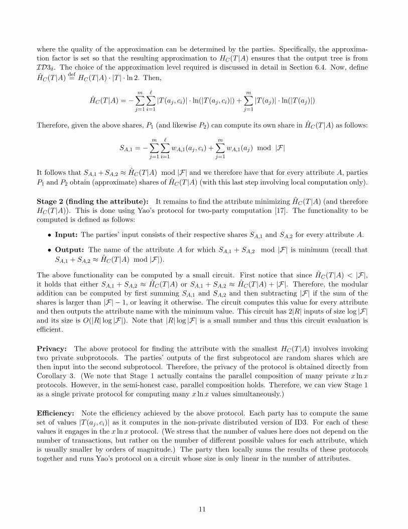
where the quality of the approximation can be determined by the parties. Specifically, the approxima-tion factor is set so that the resulting approximation to HC(T |A) ensures that the output tree is fromID3δ. The choice of the approximation level required is discussed in detail in Section 6.4. Now, defineHC(T |A) def= HC(T |A) · |T | · ln 2. Then,

HC(T |A) = −m∑

j=1

∑

i=1

|T (aj , ci)| · ln(|T (aj , ci)|) +m∑

j=1

|T (aj)| · ln(|T (aj)|)

Therefore, given the above shares, P1 (and likewise P2) can compute its own share in HC(T |A) as follows:

SA,1 = −m∑

j=1

∑

i=1

wA,1(aj , ci) +m∑

j=1

wA,1(aj) mod |F|

It follows that SA,1 +SA,2 ≈ HC(T |A) mod |F| and we therefore have that for every attribute A, partiesP1 and P2 obtain (approximate) shares of HC(T |A) (with this last step involving local computation only).

Stage 2 (finding the attribute): It remains to find the attribute minimizing HC(T |A) (and thereforeHC(T |A)). This is done using Yao’s protocol for two-party computation [17]. The functionality to becomputed is defined as follows:

• Input: The parties’ input consists of their respective shares SA,1 and SA,2 for every attribute A.

• Output: The name of the attribute A for which SA,1 + SA,2 mod |F| is minimum (recall thatSA,1 + SA,2 ≈ HC(T |A) mod |F|).

The above functionality can be computed by a small circuit. First notice that since HC(T |A) < |F|,it holds that either SA,1 + SA,2 ≈ HC(T |A) or SA,1 + SA,2 ≈ HC(T |A) + |F|. Therefore, the modularaddition can be computed by first summing SA,1 and SA,2 and then subtracting |F| if the sum of theshares is larger than |F| − 1, or leaving it otherwise. The circuit computes this value for every attributeand then outputs the attribute name with the minimum value. This circuit has 2|R| inputs of size log |F|and its size is O(|R| log |F|). Note that |R| log |F| is a small number and thus this circuit evaluation isefficient.

Privacy: The above protocol for finding the attribute with the smallest HC(T |A) involves invokingtwo private subprotocols. The parties’ outputs of the first subprotocol are random shares which arethen input into the second subprotocol. Therefore, the privacy of the protocol is obtained directly fromCorollary 3. (We note that Stage 1 actually contains the parallel composition of many private x ln xprotocols. However, in the semi-honest case, parallel composition holds. Therefore, we can view Stage 1as a single private protocol for computing many x ln x values simultaneously.)

Efficiency: Note the efficiency achieved by the above protocol. Each party has to compute the sameset of values |T (aj , ci)| as it computes in the non-private distributed version of ID3. For each of thesevalues it engages in the x ln x protocol. (We stress that the number of values here does not depend on thenumber of transactions, but rather on the number of different possible values for each attribute, whichis usually smaller by orders of magnitude.) The party then locally sums the results of these protocolstogether and runs Yao’s protocol on a circuit whose size is only linear in the number of attributes.

11

Privacy-Preserving Protocol for ID3:

Step 1: If R is empty, return a leaf-node with the class value assigned to the most transactions in T .Since the set of attributes is known to both parties, they both publicly know if R is empty. If yes, theparties run Yao’s protocol for the following functionality: Parties 1 and 2 input (|T1(c1)|, . . . , |T1(c`)|)and (|T2(c1)|, . . . , |T2(c`)|) respectively. The output is the class index i for which |T1(ci)| + |T2(ci)| islargest. The size of the circuit computing the above functionality is linear in ` and log |T |.

Step 2: If T consists of transactions which all have the same value c for the class attribute, return a leaf-nodewith the value c.In order to compute this step privately, we must determine whether both parties remain with the samesingle class or not. We define a fixed symbol ⊥ symbolizing the fact that a party has more than oneremaining class. A party’s input to this step is then ⊥, or ci if it is its one remaining class. All thatremains to do is check equality of the two inputs. The value causing the equality can then be publiclyannounced as ci (halting the tree on this path) or ⊥ (to continue growing the tree from the currentpoint). For efficient secure protocols for checking equality, see [7, 13] or simply run Yao’s protocol witha circuit for testing equality.

Step 3: (a) Determine the attribute that best classifies the transactions in T , let it be A.For every value aj of every attribute A, and for every value ci of the class attribute C, the parties runthe x ln x protocol of Section 6 for |T (aj)| and |T (aj , ci)|. They then continue as described in Section 5.2by computing independent additions, and inputting the results into Yao’s protocol for a small circuitcomputing the attribute with the highest information gain. This attribute is public knowledge as itbecomes part of the output.(b,c) Recursively call ID3δ for the remaining attributes on the transaction sets T (a1), . . . , T (am) (wherea1, . . . , am are the values of attribute A).The result of 3(a) and the attribute values of A are public and therefore both parties can individuallypartition the database and prepare their input for the recursive calls.

Figure 2: Protocol for Privately Computing ID3δ

5.3 The Private ID3δ Protocol

In the previous subsection we showed how each node can be privately computed. The complete protocolfor privately computing ID3δ can be seen in Figure 2. The steps of the protocol correspond to those inthe original algorithm (see Figure 1).

Although each individual step of the complete protocol is private, we must show that the compositionis also private. Recall that the composition theorem (Theorem 2) only states that if the oracle-aidedprotocol is private, then so too is the protocol for which we use private protocols instead of oracles. Herewe prove that the oracle-aided ID3δ protocol is indeed private.

The central issue in the proof involves showing that despite the fact that the control flow depends onthe input (and is not predetermined), a simulator can exactly predict the control flow of the protocolfrom the output. This is non-trivial and in fact, as we remark below, were we to switch Steps (1) and(2) in the protocol (as the algorithm is in fact presented in [12]) the protocol would no longer be private.Formally, of course, we show how the simulator generates a party’s view based solely on the input andoutput.

Theorem 4 The protocol for computing ID3δ is private.

Proof: In this proof the simulator is described in generic terms as it is identical for P1 and P2. Fur-thermore, we skip details which are obvious. Recall that the simulator is given the output decisiontree.

12

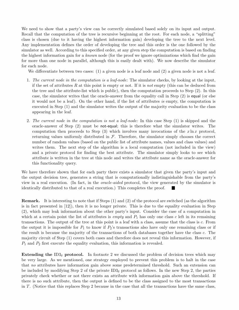
We need to show that a party’s view can be correctly simulated based solely on its input and output.Recall that the computation of the tree is recursive beginning at the root. For each node, a “splitting”class is chosen (due to it having the highest information gain) developing the tree to the next level.Any implementation defines the order of developing the tree and this order is the one followed by thesimulator as well. According to this specified order, at any given step the computation is based on findingthe highest information gain for a known node (for the proof we ignore optimizations which find the gainfor more than one node in parallel, although this is easily dealt with). We now describe the simulatorfor each node.

We differentiate between two cases: (1) a given node is a leaf node and (2) a given node is not a leaf.

1. The current node in the computation is a leaf-node: The simulator checks, by looking at the input,if the set of attributes R at this point is empty or not. If it is not empty (this can be deduced fromthe tree and the attribute-list which is public), then the computation proceeds to Step (2). In thiscase, the simulator writes that the oracle-answer from the equality call in Step (2) is equal (or elseit would not be a leaf). On the other hand, if the list of attributes is empty, the computation isexecuted in Step (1) and the simulator writes the output of the majority evaluation to be the classappearing in the leaf.

2. The current node in the computation is not a leaf-node: In this case Step (1) is skipped and theoracle-answer of Step (2) must be not-equal; this is therefore what the simulator writes. Thecomputation then proceeds to Step (3) which involves many invocations of the x lnx protocol,returning values uniformly distributed in F . Therefore, the simulator simply chooses the correctnumber of random values (based on the public list of attribute names, values and class values) andwrites them. The next step of the algorithm is a local computation (not included in the view)and a private protocol for finding the best attribute. The simulator simply looks to see whichattribute is written in the tree at this node and writes the attribute name as the oracle-answer forthis functionality query.

We have therefore shown that for each party there exists a simulator that given the party’s input andthe output decision tree, generates a string that is computationally indistinguishable from the party’sview in a real execution. (In fact, in the oracle-aided protocol, the view generated by the simulator isidentically distributed to that of a real execution.) This completes the proof.

Remark. It is interesting to note that if Steps (1) and (2) of the protocol are switched (as the algorithmis in fact presented in [12]), then it is no longer private. This is due to the equality evaluation in Step(2), which may leak information about the other party’s input. Consider the case of a computation inwhich at a certain point the list of attributes is empty and P1 has only one class c left in its remainingtransactions. The output of the tree at this point is a leaf with a class, assume that the class is c. Fromthe output it is impossible for P1 to know if P2’s transactions also have only one remaining class or ifthe result is because the majority of the transactions of both databases together have the class c. Themajority circuit of Step (1) covers both cases and therefore does not reveal this information. However, ifP1 and P2 first execute the equality evaluation, this information is revealed.

Extending the ID3δ protocol. In footnote 2 we discussed the problem of decision trees which maybe very large. As we mentioned, one strategy employed to prevent this problem is to halt in the casethat no attributes have information gain above some predetermined threshold. Such an extension canbe included by modifying Step 2 of the private ID3δ protocol as follows. In the new Step 2, the partiesprivately check whether or not there exists an attribute with information gain above the threshold. Ifthere is no such attribute, then the output is defined to be the class assigned to the most transactionsin T . (Notice that this replaces Step 2 because in the case that all the transactions have the same class,

13

the information gain for every attribute equals zero.) As in Step 3, most of the work involves computingshares of HC(T |A). These shares (along with shares of HC(T )) are then input into a circuit that outputsthe desired functionality. Of course, in order to improve efficiency, Steps 2 and 3 should then be combinedtogether.

5.4 Complexity

The complexity (measuring both communication and computational complexity) for each node is asfollows (recall that R denotes the set of attributes and T the set of transactions):

• The x lnx protocol is repeated m(` + 1) times for each attribute where m and ` are the numberof attribute and class values respectively (see Eq. (3)). For all |R| attributes we thus have O(m ·` · |R|) invocations of the x lnx protocol. The complexity of the x lnx protocol can be found inSection 6.3. In short, the computational overhead of the x ln x protocol is dominated by O(log |T |)oblivious transfers and the bandwidth is O(k · log |T | · |S|) bits, where k is a parameter dependinglogarithmically on δ that determines the accuracy of the x ln x approximation and |S| is the lengthof the key for a pseudorandom function (say 128 bits).

• As we have mentioned, the size of the circuit computing the attribute with the minimum conditionalentropy is O(|R| log |F|) where |F| = O(|T |).5 The bandwidth involved in sending the garbled circuitof Yao’s protocol is thus O(|R| log |T | · |S|) where |S| is the length of the key for a pseudorandomfunction. (This factor is explained in the paragraph titled “overhead” in Appendix B.)

The computational complexity of the above circuit evaluation involves |R| log |F| = O(|R| log |T |)oblivious transfers (one for each bit of the circuit input) and O(|R| log |T |) pseudorandom functionevaluations.

• The number of rounds needed for each node is constant (the x ln x protocol also requires only aconstant number of rounds, see Section 6).

The overhead of the x lnx invocations far outweighs the circuit evaluation that completes the computa-tion. We thus consider only these invocations in the overall complexity. The analysis is completed bymultiplying the above complexity by the number of nodes in the resulting decision tree (expected to bequite small).6 We note that by computing nodes on the same level of the tree in parallel, the number ofrounds of communication can be reduced to the order of the depth of the tree (which is bounded by |R|but is expected to be far smaller).

Comparison to non-private distributed ID3. We conclude by comparing the communication com-plexity to that of the non-private distributed ID3 protocol (see Section 5.1). In the non-private case, thebandwidth for each node is exactly |R|m` log |T | bits. On the other hand, in order to achieve a privateprotocol, an additional multiplicative factor of k · |S| is incurred (plus the constants incurred by the x ln xand Yao protocols). Thus, the communication complexity of the private protocol is reasonably close tothat of its non-private counterpart.

5We note that the size of the field F needed for the x ln x protocol is actually larger than that required for this part ofthe protocol. As is described in Section 6, log |F| = O(k log |T |) where k is a parameter depending on δ as described above.However, k ≈ 12 provides high accuracy and therefore this does not make a significant difference.

6Note that the overhead is actually even smaller since the effective number of attributes in a node of depth d′ is |R| − d′.Since most nodes are at lower levels of the tree and since this is a multiplicative factor in the expression of the overhead, theoverhead is decreased substantially. The effective value of |R| for the overall overhead can be reduced to about |R| minusthe depth of the resulting decision tree.

14

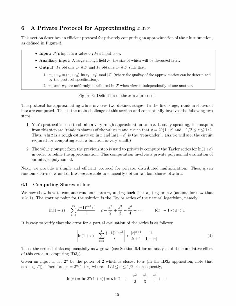
6 A Private Protocol for Approximating x ln x

This section describes an efficient protocol for privately computing an approximation of the x ln x function,as defined in Figure 3.

• Input: P1’s input is a value v1; P2’s input is v2.

• Auxiliary input: A large enough field F , the size of which will be discussed later.

• Output: P1 obtains w1 ∈ F and P2 obtains w2 ∈ F such that:

1. w1+w2 ≈ (v1+v2)·ln(v1+v2) mod |F| (where the quality of the approximation can be determinedby the protocol specification),

2. w1 and w2 are uniformly distributed in F when viewed independently of one another.

Figure 3: Definition of the x ln x protocol.

The protocol for approximating x lnx involves two distinct stages. In the first stage, random shares oflnx are computed. This is the main challenge of this section and conceptually involves the following twosteps:

1. Yao’s protocol is used to obtain a very rough approximation to lnx. Loosely speaking, the outputsfrom this step are (random shares) of the values n and ε such that x = 2n(1+ε) and −1/2 ≤ ε ≤ 1/2.Thus, n ln 2 is a rough estimate on lnx and ln(1+ε) is the “remainder”. (As we will see, the circuitrequired for computing such a function is very small.)

2. The value ε output from the previous step is used to privately compute the Taylor series for ln(1+ε)in order to refine the approximation. This computation involves a private polynomial evaluation ofan integer polynomial.

Next, we provide a simple and efficient protocol for private, distributed multiplication. Thus, givenrandom shares of x and of lnx, we are able to efficiently obtain random shares of x ln x.

6.1 Computing Shares of ln x

We now show how to compute random shares u1 and u2 such that u1 + u2 ≈ ln x (assume for now thatx ≥ 1). The starting point for the solution is the Taylor series of the natural logarithm, namely:

ln(1 + ε) =∞∑

i=1

(−1)i−1εi

i= ε− ε2

2+

ε3

3− ε4

4+ · · · for − 1 < ε < 1

It is easy to verify that the error for a partial evaluation of the series is as follows:∣∣∣∣∣ln(1 + ε)−

k∑

i=1

(−1)i−1εi

i

∣∣∣∣∣ <|ε|k+1

k + 1· 11− |ε| (4)

Thus, the error shrinks exponentially as k grows (see Section 6.4 for an analysis of the cumulative effectof this error in computing ID3δ).

Given an input x, let 2n be the power of 2 which is closest to x (in the ID3δ application, note thatn < log |T |). Therefore, x = 2n(1 + ε) where −1/2 ≤ ε ≤ 1/2. Consequently,

ln(x) = ln(2n(1 + ε)) = n ln 2 + ε− ε2

2+

ε3

3− ε4

4+ · · ·

15

Our aim is to compute this Taylor series to the k’th place. Let N be a predetermined (public) upper-bound on the value of n (N > n always). In order to do this, we first use Yao’s protocol to privatelyevaluate a small circuit that receives as input v1 and v2 such that v1+v2 = x (the value of N is hardwiredinto the circuit), and outputs random shares of the following values:

• 2N · n ln 2 (for computing the first element in the series of lnx)

• ε · 2N (for computing the remainder of the series).

This circuit is easily constructed: notice that ε · 2n = x − 2n, where n can be determined by looking atthe two most significant bits of x, and ε · 2N is obtained simply by shifting the result by N − n bits tothe left. The possible values of 2Nn ln 2 are hardwired into the circuit. (Actually, the values here arealso approximations. However, they may be made arbitrarily close to the true values and we thereforeignore this factor from here on.) Therefore, following this step the parties have shares α1, β1 and α2, β2

such that,α1 + α2 = ε2N and β1 + β2 = 2Nn ln 2

and the shares αi and βi are uniformly distributed in the finite field F (unless otherwise specified, allarithmetic is in this field). The above is correct for the case of x ≥ 1. However, if x = 0, then x cannotbe written as 2n(1 + ε) for −1/2 ≤ ε ≤ 1/2. Therefore, the circuit is modified to simply output shares ofzero for both values in the case of x = 0 (i.e., α1 + α2 = 0 and β1 + β2 = 0).

The second step of the protocol involves computing shares of the Taylor series approximation. In fact, itcomputes shares of

lcm(2, ...k) · 2N

(n ln 2 + ε− ε2

2+

ε3

3− · · · ε

k

k

)≈ lcm(2, ...k) · 2N · ln x (5)

(where lcm(2, ..., k) is the lowest common multiple of {2, . . . , k}, and we multiply by it to ensure thatthere are no fractions). In order to do this P1 defines the following polynomial:

Q(z) = lcm(2, . . . , k) ·k∑

i=1

(−1)i−1

2N(i−1)

(α1 + z)i

i− z1

where z1 ∈R F is randomly chosen. It is easy to see that

z2def= Q(α2) = lcm(2, ..., k) · 2N ·

(k∑

i=1

(−1)i−1εi

i

)− z1

Therefore after a single private polynomial evaluation of the k-degree polynomial Q(·), parties P1 andP2 obtain random shares z1 and z2 to the approximation in Eq. (5). Namely P1 defines u1 = z1 +lcm(2, . . . , k)β1 and likewise P2. We conclude that

u1 + u2 ≈ lcm(2, . . . , k) · 2N · ln x

This equation is accurate up to an approximation error which depends on k, and the shares are random asrequired. Since N and k are known to both parties, the additional multiplicative factor of 2N ·lcm(2, . . . , k)is public and can be removed at the end (if desired). Notice that all the values in the computation areintegers (except for 2Nn ln 2 which is given as the closest integer).

16

The size of the field F . It is necessary that the field be chosen large enough so that the initial inputsin each evaluation and the final output be between 0 and |F| − 1. Notice that all computation is basedon ε2N . This value is raised to powers up to k and multiplied by lcm(2, . . . , k). Therefore a field ofsize 2Nk+2k is large enough, and requires Nk + 2k bits for representation. (This calculation is based onbounding lcm(2, . . . , k) by ek < 22k.)

We now summarize the lnx protocol (recall that N is a public upper bound on log |T |):Protocol 1 (Protocol lnx)

• Input: P1 and P2 have respective inputs v1 and v2 such that v1 + v2 = x. Denote x = 2n(1 + ε)for n and ε as described above.

• The protocol:

1. P1 and P2, upon input v1 and v2 respectively, run Yao’s protocol for a circuit that outputs thefollowing: (1) Random shares α1 and α2 such that α1 + α2 = ε2N mod|F|, and (2) Randomshares β1,β2 such that β1 + β2 = 2N · n ln 2 mod|F|.

2. P1 chooses z1 ∈R F and defines the following polynomial

Q(z) = lcm(2, . . . , k) ·k∑

i=1

(−1)i−1

2N(i−1)

(α1 + z)i

i− z1

3. P1 and P2 then execute a private polynomial evaluation with P1 inputting Q(·) and P2 in-putting α2, in which P2 obtains z2 = Q(α2).

4. P1 and P2 define u1 = lcm(2, . . . , k)β1 + z1 and u2 = lcm(2, . . . , k)β2 + z2, respectively. Wehave that u1 + u2 ≈ lcm(2, . . . , k) · 2N · lnx

We now prove that the lnx protocol is correct and secure. We prove correctness by showing that thefield and intermediate values are such that the output shares uniquely define the result. On the otherhand, privacy is derived directly from Corollary 3.

Before beginning the proof, we introduce notation for measuring the accuracy of the approximation.That is, we say that x is a ∆-approximation of x if |x− x| ≤ ∆.

Proposition 5 Protocol 1 constitutes a private protocol for computing random shares of a c2k(k+1)

-

approximation of c · ln x in F , where c = lcm(2, . . . , k) · 2N .

Proof: We begin by showing that the protocol correctly computes shares of an approximation of c ln x.In order to do this, we must show that the computation over F results in a correct result over the reals.We first note that all the intermediate values are integers. In particular, ε2n equals x−2n and is thereforean integer as is ε2N (since N > n). Furthermore, every division by i (2 ≤ i ≤ k) is counteracted by amultiplication by lcm(2, . . . , k). The only exception is 2Nn ln 2. However, this is taken care of by havingthe original circuit output the closest integer to 2Nn ln 2.

Secondly, the field F is defined to be large enough so that all intermediate values (i.e. the sum ofshares) and the final output (as a real number times lcm(2, . . . , k) · 2N ) are between 0 and |F| − 1.Therefore the two shares uniquely identify the result, which equals the sum (over the integers) of the tworandom shares if it is less than |F| − 1, or the sum minus |F| otherwise.

Finally, we show that the accuracy of the approximation is as desired. As we have mentioned inEq. (4), the ln(1 + ε) error is bounded by |ε|k+1

k+11

1−|ε| . Since −12 ≤ ε ≤ 1

2 , we have that this error rate is

maximum at |ε| = 12 . We therefore have that

∣∣∣ln(1 + ε)− ln(1 + ε)∣∣∣ ≤ 1

2k(k+1), where ln(1 + ε) denotes

17

the approximation of the lnx protocol. Now, c ln x = cn ln 2 + c ln(1 + ε) and therefore by adding cn ln 2to both c ln(1 + ε) and cln(1 + ε) we have that this has no effect on the error. (We note that we actuallyadd an approximation of cn ln 2 to cln(1+ε) in the protocol. Nevertheless, the error of this approximationcan be made to be much smaller than c

2k(k+1). This is because the approximation of 2Nn ln 2 is hardwired

into the circuit as the closest integer, and thus by increasing N the error can be made as small as desired.)Therefore, the total error of clnx is c

2k(k+1), which means that the effective error of the approximation of

lnx is only 12k(k+1)

.

Privacy: The fact that the lnx protocol is private is derived directly from Corollary 3. Recall thatthis lemma states that a protocol composed of two private protocols, where the first one outputs randomshares only, is private. The lnx protocol is constructed in exactly this way and thus the privacy followsfrom the lemma.

6.2 Computing Shares of x ln x

We begin by describing a multiplication protocol that on private inputs a1 and a2 outputs random sharesb1 and b2 (in some finite field F) such that b1 + b2 = a1 · a2. The protocol is very simple and is based ona single private evaluation of a linear polynomial.

Protocol 2 (Protocol Mult(a1, a2))

1. P1 chooses a random value b1 ∈ F and defines the linear polynomial Q(z) = a1z − b1.

2. P1 and P2 engage in a private evaluation of Q, in which P2 obtains b2 = Q(a2) = a1 · a2 − b1.

3. The respective outputs of P1 and P2 are defined as b1 and b2, giving us that b1 + b2 = a1 · a2.

The correctness of the protocol (i.e., that b1 and b2 are uniformly distributed in F and sum up to a1 ·a2) isimmediate from the definition of Q. Furthermore, the privacy follows from the privacy of the polynomialevaluation. We thus have the following proposition:

Proposition 6 Protocol 2 constitutes a private protocol for computing Mult as defined above.

We are now ready to present the complete x ln x protocol (recall that P1 and P2’s respective inputsare v1 and v2 where v1 + v2 = x):

Protocol 3 (Protocol x lnx)

1. P1 and P2 run Protocol 1 for privately computing shares of lnx and obtain random shares u1 andu2 such that u1 + u2 ≈ ln x.

2. P1 and P2 use two invocations of Protocol 2 in order to obtain shares of u1 · v2 and u2 · v1.

3. P1 (resp., P2) then defines his output w1 (resp., w2) to be the sum of the two Mult shares and u1 ·v1

(resp., u2 · v2).

4. We have that w1 + w2 = u1v1 + u1v2 + u2v1 + u2v2 = (u1 + u2)(v1 + v2) ≈ x ln x as required.

Applying Corollary 3 we obtain the following theorem:

Theorem 7 Protocol 3 is a private protocol for computing random shares of x lnx.

18

6.3 Complexity

The lnx Protocol (Protocol 1):

1. Step 1 of the protocol (computing random shares α1, α2, β1 and β2) involves running Yao’s protocolon a circuit that is linear in the size of v1 and v2 (these values are of size at most log |T |). Thebandwidth involved in sending the garbled circuit in Yao’s protocol is O(log |F||S|) = O(k log |T |·|S|)communication bits where |S| is the length of the key for a pseudorandom function. (This isexplained in Appendix B.)

The computational complexity is dominated by the oblivious transfers that are required for everybit of the circuit input. Since the size of the circuit input is at most 2 log |T |, this upper boundsthe number of oblivious transfers required.

2. Steps 2 and 3 of the protocol (computing the Taylor series) involve the private evaluation of apolynomial of degree k over the field F . This private evaluation can be computed using O(k)exponentiations and O(k) messages of total length O(k|E|) where |E| is the length of an elementin the group in which the oblivious transfers and exponentiations are implemented.

The overall computation overhead of the protocol is thus O(max{log |T |, k}) exponentiations. Since |T |is usually large (e.g. log |T | = 20), and on the other hand k can be set to small values (e.g. k = 12,see below), the computational overhead can be defined as O(log |T |) oblivious transfers. The maincommunication overhead is incurred by Step 1, and is O(k log |T | · |S|) bits.

The Mult Protocol (Protocol 2): This protocol involves a single oblivious evaluation of a linearpolynomial by the players.

The x ln x Protocol (Protocol 3): This step involves one invocation of Protocol 1, and two invoca-tions of Protocol 2. Its overhead is therefore dominated by Protocol 1. We conclude that the overallcomputational complexity is O(log |T |) oblivious transfers and that the bandwidth is O(k log |T | · |S|)bits.

6.4 Choosing the Parameter k for the Approximation

Recall that the parameter k defines the accuracy of the Taylor approximation of the “ln” function. Givenδ, we analyze the value of k needed in order to ensure that the defined δ-approximation is correctlyestimated. From here on we denote an approximation of a value z by z. The approximation definition ofID3δ requires that if an attribute A′ is chosen for any given node, then |HC(T |A′)−HC(T |A)| ≤ δ, whereA denotes the attribute with the maximum information gain. In order to ensure that only attributesthat are δ-close to A are chosen, it is sufficient to have that for all pairs of attributes A and A′

HC(T |A′) > HC(T |A) + δ ⇒ HC(T |A′) > HC(T |A) (6)

This is enough because the attribute A′ chosen by our specific protocol is that which has the smallestHC(T |A′). If Eq. (6) holds, then we are guaranteed that HC(T |A′)−HC(T |A) ≤ δ as required (becauseotherwise we would have that HC(T |A′) > HC(T |A) and then A′ would not have been chosen). Eq. (6)is fulfilled if the approximation is such that for every attribute A,

∣∣∣HC(T |A)− HC(T |A)∣∣∣ <

δ

2

We now bound the difference on each | ln x−lnx| in order that the above condition is fulfilled. By replacinglog x by 1

ln 2 | lnx− lnx| in Eq. (3) computing HC(T |A) (see Section 5.1), we obtain a bound on the errorof

∣∣∣HC(T |A)− HC(T |A)∣∣∣. A straightforward algebraic manipulation gives us that if 1

ln 2 | ln x− lnx| < δ4 ,

19

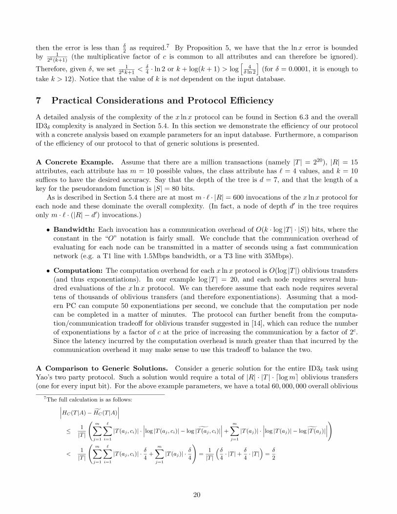
then the error is less than δ2 as required.7 By Proposition 5, we have that the lnx error is bounded

by 12k(k+1)

(the multiplicative factor of c is common to all attributes and can therefore be ignored).

Therefore, given δ, we set 12kk+1

< δ4 · ln 2 or k + log(k + 1) > log

[4

δ ln 2

](for δ = 0.0001, it is enough to

take k > 12). Notice that the value of k is not dependent on the input database.

7 Practical Considerations and Protocol Efficiency

A detailed analysis of the complexity of the x ln x protocol can be found in Section 6.3 and the overallID3δ complexity is analyzed in Section 5.4. In this section we demonstrate the efficiency of our protocolwith a concrete analysis based on example parameters for an input database. Furthermore, a comparisonof the efficiency of our protocol to that of generic solutions is presented.

A Concrete Example. Assume that there are a million transactions (namely |T | = 220), |R| = 15attributes, each attribute has m = 10 possible values, the class attribute has ` = 4 values, and k = 10suffices to have the desired accuracy. Say that the depth of the tree is d = 7, and that the length of akey for the pseudorandom function is |S| = 80 bits.

As is described in Section 5.4 there are at most m · ` · |R| = 600 invocations of the x ln x protocol foreach node and these dominate the overall complexity. (In fact, a node of depth d′ in the tree requiresonly m · ` · (|R| − d′) invocations.)

• Bandwidth: Each invocation has a communication overhead of O(k · log |T | · |S|) bits, where theconstant in the “O” notation is fairly small. We conclude that the communication overhead ofevaluating for each node can be transmitted in a matter of seconds using a fast communicationnetwork (e.g. a T1 line with 1.5Mbps bandwidth, or a T3 line with 35Mbps).

• Computation: The computation overhead for each x lnx protocol is O(log |T |) oblivious transfers(and thus exponentiations). In our example log |T | = 20, and each node requires several hun-dred evaluations of the x lnx protocol. We can therefore assume that each node requires severaltens of thousands of oblivious transfers (and therefore exponentiations). Assuming that a mod-ern PC can compute 50 exponentiations per second, we conclude that the computation per nodecan be completed in a matter of minutes. The protocol can further benefit from the computa-tion/communication tradeoff for oblivious transfer suggested in [14], which can reduce the numberof exponentiations by a factor of c at the price of increasing the communication by a factor of 2c.Since the latency incurred by the computation overhead is much greater than that incurred by thecommunication overhead it may make sense to use this tradeoff to balance the two.

A Comparison to Generic Solutions. Consider a generic solution for the entire ID3δ task usingYao’s two party protocol. Such a solution would require a total of |R| · |T | · dlog me oblivious transfers(one for every input bit). For the above example parameters, we have a total 60, 000, 000 overall oblivious

7The full calculation is as follows:∣∣∣HC(T |A)− HC(T |A)

∣∣∣

≤ 1

|T |

(m∑

j=1

∑i=1

|T (aj , ci)| ·∣∣∣log |T (aj , ci)| − ˜log |T (aj , ci)|

∣∣∣ +

m∑j=1

|T (aj)| ·∣∣∣log |T (aj)| − ˜log |T (aj)|

∣∣∣)

<1

|T |

(m∑

j=1

`∑i=1

|T (aj , ci)| · δ

4+

m∑j=1

|T (aj)| · δ

4

)=

1

|T |(

δ

4· |T |+ δ

4· |T |

)=

δ

2

20

transfers. Furthermore, as the number of transactions |T | grows, the gap between the complexity of thegeneric protocol and the complexity of our protocol grows rapidly, since the overhead of our protocol isonly logarithmic in |T |. The size of the circuit sent in the generic protocol is also at least O(|R| · |T | · |S|)(a very optimistic estimate) which is once again much larger than in our protocol.

Consider now a semi-generic solution for which the protocol is exactly as described in Figure 2.However, a generic (circuit-based) solution is used for the x ln x protocol instead of the protocol ofSection 6. This generic protocol should compute the Taylor series, namely k multiplications in F , witha communication overhead of O(k log2 |F||S|) = O(k3 log2 |T ||S|) (circuit multiplication is quadratic inthe length of the inputs). This is larger by a factor of k2 log |T | than the communication overhead of ourprotocol. On the other hand, the number of oblivious transfers would remain much the same in bothcases, and this overhead dominates the computation overhead of both protocols.

Acknowledgements

We would like to thank the anonymous referees for their many helpful comments.

References

[1] M. Ben-Or, S. Goldwasser and A. Wigderson, Completeness theorems for non cryptographic faulttolerant distributed computation, Proceedings of the 20th Annual Symposium on the Theory ofComputing (STOC), ACM, 1988, pp. 1–9.

[2] D. Boneh and M. Franklin, Efficient generation of shared RSA keys, Advances in Cryptology -CRYPTO ’97. Lecture Notes in Computer Science, Vol. 1233, Springer-Verlag, 1997, pp. 425–439.

[3] R. Canetti, Security and Composition of Multi-party Cryptographic Protocols, Journal of Cryptol-ogy, Vol. 13, No. 1, 2000, pp. 143–202.

[4] D. Chaum, C. Crepeau and I. Damgard, Multiparty unconditionally secure protocols, Proceedingsof the 20th Annual Symposium on the Theory of Computing (STOC), ACM, 1988, pp. 11–19.

[5] B. Chor, O. Goldreich, E. Kushilevitz and M. Sudan, Private Information Retrieval, Proceedings36th Symposium on Foundations of Computer Science (FOCS), IEEE, 1995, pp. 41–50.

[6] S. Even, O. Goldreich and A. Lempel, A Randomized Protocol for Signing Contracts, Communica-tions of the ACM, vol. 28, 1985, pp. 637–647.

[7] R. Fagin, M. Naor and P. Winkler, Comparing Information Without Leaking It, Communicationsof the ACM, vol. 39, 1996, pp. 77–85.

[8] J. Feigenbaum, Y. Ishai, T. Malkin, K. Nissim, M. Strauss, and R. Wright, Secure MultipartyComputation of Approximations, 28th International Colloquium on Automata, Languages and Pro-gramming (ICALP), 2001, pp. 927–938.

[9] O. Goldreich, Secure Multi-Party Computation. Manuscript, 1998. (Available athttp://www.wisdom.weizmann.ac.il/∼oded/pp.html)

[10] O. Goldreich, S. Micali and A. Wigderson, How to Play any Mental Game - A Completeness Theoremfor Protocols with Honest Majority., Proceedings of the 19th Annual Symposium on the Theory ofComputing (STOC), ACM, 1987, pp. 218–229.

21

[11] Y. Lindell and B. Pinkas, Privacy Preserving Data Mining, Advances in Cryptology - CRYPTO ’00.Lecture Notes in Computer Science, Vol. 1880, Springer-Verlag, 2000, pp. 36–53. Earlier version ofthis paper.

[12] T. Mitchell, Machine Learning. McGraw Hill, 1997.

[13] M. Naor and B. Pinkas, Oblivious Transfer and Polynomial Evaluation, Proceedings of the 31thAnnual Symposium on the Theory of Computing (STOC), ACM, 1999, pp. 245–254.

[14] M. Naor and B. Pinkas, Efficient Oblivious Transfer Protocols, Proceedings of 12th SIAM Symposiumon Discrete Algorithms (SODA), January 7-9 2001, Washington DC, pp. 448–457.

[15] J. Ross Quinlan, Induction of Decision Trees, Machine Learning 1(1), 1986, pp. 81–106.

[16] M. O. Rabin, How to exchange secrets by oblivious transfer, Technical Memo TR-81, Aiken Com-putation Laboratory, 1981.

[17] A. C. Yao, How to generate and exchange secrets, Proceedings 27th Symposium on Foundations ofComputer Science (FOCS), IEEE, 1986, pp. 162–167.

A A Decision Tree Example

In this appendix we give an example of a data set and the resulting decision tree. (The examples aretaken from Chapter 3 of Tom Mitchell’s book Machine Learning, see [12].) The aim of the task here isto learn the weather conditions suitable for playing tennis.

Day Outlook Temperature Humidity Wind Play TennisD1 Sunny Hot High Weak NoD2 Sunny Hot High Strong NoD3 Overcast Hot High Weak YesD4 Rain Mild High Weak YesD5 Rain Cool Normal Weak YesD6 Rain Cool Normal Strong NoD7 Overcast Cool Normal Strong YesD8 Sunny Mild High Weak NoD9 Sunny Cool Normal Weak YesD10 Rain Mild Normal Weak YesD11 Sunny Mild Normal Strong YesD12 Overcast Mild High Strong YesD13 Overcast Hot Normal Weak YesD14 Rain Mild High Strong No

The first attribute chosen in the tree for the above database is Outlook. This is seen by a quickcomputation of the Gain. By a quick calculation one can confirm that Gain(T, Outlook) = 0.246 whichis maximum over the gain of all other attributes. We can see the entropy gain calculation for one of thelower nodes in the tree below.

22

Outlook

Sunny Overcast Rain

[9+,5−]

{D1,D2,D8,D9,D11} {D3,D7,D12,D13} {D4,D5,D6,D10,D14}

[2+,3−] [4+,0−] [3+,2−]

Yes

{D1, D2, ..., D14}

? ?

Which attribute should be tested here?

Ssunny = {D1,D2,D8,D9,D11}

Gain (Ssunny , Humidity)

sunnyGain (S , Temperature) = .970 − (2/5) 0.0 − (2/5) 1.0 − (1/5) 0.0 = .570

Gain (S sunny , Wind) = .970 − (2/5) 1.0 − (3/5) .918 = .019

= .970 − (3/5) 0.0 − (2/5) 0.0 = .970

It is clear that “Humidity” is the best choice by its Gain value. Intuitively, this is logical as itcompletes the classification in the most concise manner (there is no need for any further tests). Below,we can see the final decision tree.

Outlook

Overcast

Humidity

NormalHigh

No Yes

Wind

Strong Weak

No Yes

Yes

RainSunny

A new transaction is then classified by traversing the tree according to the attribute/values. For example,the transaction:

(Outlook = Sunny, Temperature = Hot, Humidity = High, Wind = Strong)

is classified as No by seeing that it is a sunny and humid day. This example demonstrates ID3’s bias infavor of short hypotheses (at most two out of the four attributes are tested).

Our aim is to output a tree such as this one, such that nothing can be learned about the other party’sdatabase that cannot be learned from the output itself.

23

B Yao’s Protocol for Private Two-Party Computation

We now describe Yao’s protocol for private two-party computation in the case that the adversary issemi-honest. Let A and B be parties with respective inputs x and y and let f be the functionality to beprivately computed by the two parties. We note that f may be a probabilistic functionality. In this briefdescription, we assume for simplicity that both A and B are to obtain the same value f(x, y).

The protocol is based on expressing f as a combinatorial circuit with gates defined over some fixedbase B (e.g., B can include all the functions g : {0, 1}×{0, 1} 7→ {0, 1}). The bits of the input are enteredinto input wires and are propagated through the gates.

Protocol for two-party secure function evaluation

Input: A and B have respective input values x and y.

Output: A and B both receive the value f(x, y).

The Protocol:

• Encrypting the circuit: A constructs an “encrypted” version of the circuit computing f asfollows. First, A hardwires its input into the circuit, thus obtaining a circuit computing f(x, ·).Then, A assigns to each wire i of the circuit two random values (W 0

i ,W 1i ) corresponding to values 0

and 1 of the wire (the random values should be long enough to be used as keys to a pseudo-randomfunction). Denote the value of the wire by bi ∈ {0, 1}. Party A also assigns to the wire a randompermutation over {0, 1}, πi : bi 7→ ci. Denote 〈W bi

i , ci〉 as the ‘garbled value’ of wire i.

Consider a gate g which computes the value of the wire k as a function of wires i and j, bk = g(bi, bj).A prepares a table Tg which enables computation of the garbled output of g, 〈W bk

k , ck〉, from thegarbled inputs to g, namely the values 〈W bi

i , ci〉, 〈W bj

j , cj〉. Given the two garbled inputs to g, thetable does not disclose information about the output of g for any other inputs, nor does it revealthe values of the bits bi, bj , bk. The table essentially encrypts the garbled value of the output wireusing the output of a pseudo-random function F keyed by the garbled values of the input wires.

The construction of Tg uses a pseudo-random function F whose output length is |W bkk | + 1 bits.

Assume that the fan out of each gate is one. The table contains four entries of the form

ci, cj : 〈(W g(bi,bj)k , ck)⊕ F

Wbii

(cj)⊕ FW

bjj

(ci)〉

for 0 ≤ i, j ≤ 1, where ci = π(bi), cj = π(bj), and ck = πk(bk) = πk(g(bi, bj)). (The entry does notinclude its index ci, cj explicitly, as it can be deduced from the location.)

To verify that the table enables B to compute the garbled output value given the garbled inputvalues, assume that B knows 〈W bi

i , ci〉, 〈W bj

j , cj〉. B should find the entry (ci, cj) in the table Tk,

and compute its exclusive-or with (FW

bii

(cj)⊕ FW

bjj

(ci)). The result is 〈W bkk = W

g(bi,bj)k , ck〉.

If the fan out of a a gate is greater than 1, care should be taken to ensure that same value is notused to mask values in different gates that have the same input. This can be done by assigning adifferent id for every gate and using this id as an input to the pseudo-random function F . Namely,a gate with id g has table entries of the form ci, cj : 〈(W g(bi,bj)

k , ck)⊕ FW

bii

(g, cj)⊕ FW

bjj

(g, ci)〉.

• Coding the input: The tables described above enables the computation of the garbled output ofevery gate from its garbled inputs. Therefore given these tables and the garbled values 〈W bi

i , ci〉 of

24

the input wires of the circuit, it is possible to compute the garbled values of its output wires. PartyB should therefore obtain the garbled values of the input wires.

For each input wire, A and B engage in a 1-out-of-2 oblivious transfer protocol in which A is thesender, whose inputs are the two garbled values of this wire, and B is the receiver, whose input isan input bit. As a result of the oblivious transfer protocol B learns the garbled value of its inputbit (and nothing about the garbled value of the other bit), and A learns nothing.

A sends to B the tables that encode the circuit gates and a translation table from the garbledvalues of the output wires to output bits.

• Computing the circuit: At the end of the oblivious transfer protocols, party B has sufficientinformation to compute the output of the circuit f(x, y) by its own. After receiving f(x, y), partyB sends A this value so that both parties obtain the output.

To show that the protocol is secure it should be proved that the view of the parties can be simulatedbased on the input and output only. The main observation regarding the security of each gate is thatevery masking value (e.g. F

Wbii

(cj)) is used only once, and that the pseudo-randomness of F ensuresthat without knowledge of the correct key these values look random. Therefore knowledge of one garbledvalue of each of the input wires discloses only a single garbled output value of the gate; the other outputvalues are indistinguishable from random to A.

As for the security of the complete circuit, the oblivious transfer protocol ensures that B learns onlya single garbled value for each input wire, and A does not learn which value it was. Inductively, B cancompute only a single garbled output value of each gate, and in particular of the circuit. The use ofpermuted bit values ck hides the values of intermediate results (i.e. of gates inside the circuit).

It is possible to adapt the protocol for circuits in which gates have more than two inputs, and evenfor wires with more than two possible values. The size of the table for a gate with ` inputs which eachcan have d values is d`.

Overhead

Note that the communication between the two parties can be done in two rounds (assuming the use of atwo-round oblivious transfer protocol [6, 9]).

Consider a circuit with n inputs and m gates. The protocol requires A to prepare m tables and sendthem to B. This is the major communication overhead of the protocol. In the case of binary gates, thecommunication overhead is 4m times the length of the output of the pseudo-random function (typically64 to 128 bits long).

The main computational overhead of the protocol is the computation of the n oblivious transfers.Afterwards party B computes the output of the circuit, and this stage involves m applications of apseudo-random function. For small circuits, the overhead of this stage is typically negligible comparedto the oblivious transfer stage.

25