probabilistic approach to slope...
TRANSCRIPT

Probabilistic Approach to Slope Stability Assessing Safety, Impact from Underlying Structures and Clay Properties in Pre Constructed Areas Master of Science Thesis in the Master’s Programme Infrastructure and Environmental Engineering
DAVID EKSTRAND PER NYLANDER Department of Civil and Environmental Engineering Division of GeoEngineering
Geotechnical Engineering Research Group
CHALMERS UNIVERSITY OF TECHNOLOGY Göteborg, Sweden 2013 Master’s Thesis 2013:53


MASTER’S THESIS 2013:53
Probabilistic Approach to Slope Stability Assessing Safety, Impact from Underlying Structures and Clay Properties in Pre
Constructed Areas Master of Science Thesis in the Master’s Programme Infrastructure and
Environmental Engineering
DAVID EKSTRAND
PER NYLANDER
Department of Civil and Environmental Engineering Division of GeoEngineering
Geotechnical Engineering Research Group CHALMERS UNIVERSITY OF TECHNOLOGY
Göteborg, Sweden 2013

Probabilistic Approach to Slope Stability Assessing Safety, Impact from Underlying Structures and Clay Properties in Pre Constructed Areas Master of Science Thesis in the Master’s Programme Infrastructure and Environmental Engineering DAVID EKSTRAND & PER NYLANDER
© DAVID EKSTRAND & PER NYLANDER, 2013
Examensarbete / Institutionen för bygg- och miljöteknik, Chalmers tekniska högskola 2013:53 Department of Civil and Environmental Engineering Division of GeoEngineering Geotechnical Engineering Research Group Chalmers University of Technology SE-412 96 Göteborg Sweden Telephone: + 46 (0)31-772 1000 Cover: Drawing of the underlying structures of the channel wall renovated in 1893 near Stora Hamnkanalen in Göteborg (Högsta, 2011). Department of Civil and Environmental Engineering Göteborg, Sweden 2013

I
Probabilistic Approach to Slope Stability Assessing Safety, Impact from Underlying Structures and Clay Properties in Pre Constructed Areas Master of Science Thesis in the Master’s Programme Infrastructure and Environmental Engineering DAVID EKSTRAND PER NYLANDER Department of Civil and Environmental Engineering Division of GeoEngineering Geotechnical Engineering Research Group Chalmers University of Technology
ABSTRACT
In this thesis a probabilistic model of the stability of a slope has been designed. The probabilistic model questions the normal assumptions made when evaluating the stability of a slope. These assumptions surround the size of traffic loads, how water levels are applied and how the effects of underlying constructions are calculated. Swedish slope stability calculation standards lack the possibility of using the favourable effects of pre-existing underlying constructions. A method to quantify the stabilising effects of underlying wooden piles was developed using existing research on horizontally loaded piles. The model also includes an investigation of the effect of anisotropic clay properties in stability investigations. The data necessary for the model was collected from previous stability investigations and soil investigation reports from a study area in the central parts of Göteborg. The model was designed with basic statistical concepts and Swedish geotechnical directives from different disciplines in the field of geotechnical engineering. The result show which assumptions that provide the greatest impact on the calculated stability of a slope. The results suggest that underlying constructions and anisotropic clay behaviour are crucial factors often neglected when calculating the factor of safety of a slope.
Key words: Anisotropic shear strength, Factor of safety, Normal distribution, Probabilistic model, Slope stability, SLOPE/W, Soft clay, Stabilising effects from wooden piles, TK Geo 11, Traffic loads, Water levels.

II

CHALMERS Civil and Environmental Engineering, Master’s Thesis 2013:53 III
Contents ABSTRACT I
CONTENTS III
PREFACE VI
NOTATIONS VII
1 INTRODUCTION 1
1.1 Background 1
1.2 Aim 1
1.3 Limitations 2
1.4 Method 2
2 THEORY 3
2.1 Soil Properties 3
2.1.1 Unit Weight 3
2.1.2 Pore Pressure 3
2.1.3 Liquid Limit 4
2.1.4 Shear Strength 4
2.2 Water Levels 6
2.2.1 The Normal Distribution 7
2.3 Soil Tests 8
2.4 Pile Properties 8
2.5 Slope Stability Model 9
2.5.1 Direct Method 9
2.5.2 Computer Aided Calculations 9
2.5.3 The Swedish Transport Administration 11
2.5.4 Swedish Commission on Slope Stability 11
2.5.5 Swedish Commission on Pile Research 12
3 SITE DESCRIPTION 13
3.1 Previous Stability Investigations 13
3.1.1 Detailed Stability Investigation, SWECO Infrastructure 13
3.1.2 Diving Inspection Hamnkanalen, FROG Marine Service 14
3.1.3 Stability Investigation, Norconsult AB 14
3.1.4 Parameters Stora Hamnkanalen, ÅF AB 14
3.2 Previous Proposed Measures 14
3.3 Slope Geometry and Boundary Conditions 15
3.3.1 Soil Properties 16
3.3.2 Upholding Forces from Piles 19
3.4 Decision Support for Measurements in Existing Slopes 24

CHALMERS, Civil and Environmental Engineering, Master’s Thesis 2013:53 IV
4 PROBABILITY MODEL 25
4.1 Inputs and Assumptions 25
4.1.1 Water Levels 26
4.1.2 Traffic Loads 31
4.1.3 Pile Forces 32
4.2 Resulting Probability Model 33
5 RESULTS 35
5.1 Resulting Plots from Probability Trees 35
5.2 Results from Decision Support Methodology 38
5.3 Evaluation of Results 39
6 DISCUSSION 41
6.1 Model 41
6.2 Input Data 41
6.2.1 Water Levels 42
6.2.2 Soil Parameters 42
6.2.3 Traffic Loads 42
6.2.4 Anisotropic Conditions 43
6.2.5 Pile Length and Pile Forces 43
6.3 Results 44
6.3.1 Part 1 44
6.3.2 Part 2 45
6.3.3 Part 3 45
6.3.4 Part 4 45
6.3.5 Part 5 45
6.3.6 Combined Model 46
6.3.7 Decision Support Methodology 46
7 CONCLUSIONS 48
8 PROPOSALS FOR FURTHER STUDIES 49
9 REFERENCES 50
10 APPENDICES 51

CHALMERS Civil and Environmental Engineering, Master’s Thesis 2013:53 V

CHALMERS, Civil and Environmental Engineering, Master’s Thesis 2013:53 VI
Preface When the work with this thesis began we had a far different conception of how the final product, that is this thesis, would be form than what it really became. The idea of designing a probabilistic model is something that emerged during the course of the project.
The model has been developed in the premises of ÅF AB in central Göteborg. The development started with a literature study of Swedish standards and regulations regarding slope stability. The early work of the project also included a collection of geotechnical investigations carried out near the channel Stora Hamnkanalen in Göteborg. The actual slope stability calculations have involved over 300 SLOPE/W models either saved or forsaken. Some calculations were forsaken due to the fact that some boundary conditions were changed along the course of the project. The results from these stability calculations have thereafter been compiled and statistically interpreted.
We would like to thank for the support from Virginia Bengtsson, Roger Oscarsson and all of the Geotechnical staff at ÅF AB and Claes Alén at Chalmers University of Technology whose support made this thesis possible.
Göteborg May 2013
David Ekstrand & Per Nylander

CHALMERS Civil and Environmental Engineering, Master’s Thesis 2013:53 VII
Notations
Roman upper case letters
pileA Area of pile in cross-section [%]
soilA Area of soil in cross-section [%]
0F Worst case factor of safety [-]
1F Normal case factor of safety [-]
2F Recommended factor of safety [-]
cF Factor of safety [-]
wallF Equivalent wall and soil load [N]
xF Horizontal load [N]
maxxF Maximum horizontal load [N]
MxF max, Maximum horizontal load due to moment capacity [N]
UxF max, Maximum horizontal load due to distributed soil load [N]
)(0 NCK Relation factor, pre-consolidation pressures [-]
L Length [m]
maxM Maximum loading moment [Nm]
RdM Designing moment capacity [Nm]
sbM Moment generated within shear body [Nm]
0N Stability factor [-]
cN Bearing capacity factor of cohesive soil [-]
dP Driving forces [N/m2]
Q Distributed load [N/m2]
yU Distributed soil load [N/m2]
W Bending moment of inertia [m3]
Roman lower case letters
uc Undrained shear strength [N/m2]
mdf Designing bending moment [N/m2]
mkf Characteristic bending moment [N/m2]
modk Moisture and load duration conversion factor [-] r Radius [m] u Pore pressure [N/m2]
Lw Liquid limit [-] z Depth [m]
failurez Shear failure depth [m]

CHALMERS, Civil and Environmental Engineering, Master’s Thesis 2013:53 VIII
Greek lower case letters
α Angle of slip surface [°] ϕ Friction angle [°]
Mγ Material partial factor [-]
Sγ Saturated unit weight [N/m3]
Uγ Unsaturated unit weight [N/m3]
σ Standard deviation [Variable]
0σ Total stresses [N/m2]
c'σ Effective stresses [N/m2]
ατ Undrained shear strength in α-direction [N/m2]
horτ Horizontal undrained shear strength [N/m]
µ Mean value [Variable]
Water levels
HHLW Highest low water in 50 years [m] HHW Highest high water in 50 years [m] HLW High low water [m] LLW Lowest low water in 50 years [m] LW Low water [m] MHW Mean high water [m] MLW Mean low water [m] NW Normal water level [m] WL Water level [m]

CHALMERS, Civil and Environmental Engineering, Master’s Thesis 2013:53 1
1 Introduction The stability of a slope can be evaluated using different methods and engineering practices. In Sweden and Göteborg the guidelines and recommendations set by the Swedish commission on slope stability is often used to assess slope stability. This report is focused on assessing safety in old slope constructions where modern slope stability guidelines indicate dangerously low stability even though the constructions have been functional for over 100 years.
1.1 Background In the central parts of Göteborg the channel Stora Hamnkanalen has long been a part of the city townscape. The stability of the northern channel wall has for some time been an area of investigation for consulting agencies in Göteborg. Measurements and calculations based on current evaluation procedure suggest that the stability of the channel wall is dangerously low. Therefore further investigation of the site, stability and soil properties is of great interest and these are investigated in this project.
Clay layers that vary in depth dominate the area on both sides of Stora Hamnkanalen in central Göteborg. The channel walls are old and not constructed with the standards that are applied today. This becomes a problem on the northern side of the channel as the wall is slightly higher but also because the clay is subjected to somewhat larger stresses from structures and traffic from a state-road. Therefore the calculated stability of the northern wall is very low and could be a risk if further construction will be planned in the area or in the case of extreme water levels.
Indications from many projects in Göteborg show that standard assumptions made when assessing design parameters may not necessarily be accurate to the situation in Göteborg. There is a lot of data from the area near Stora Hamnkanalen that will be subject for further investigation, making this project a case study of the area near Stora Hamnkanalen, with additional inputs from other areas in Göteborg for comparisons and further understanding.
1.2 Aim The aim of the project is to get a greater understanding of the correlation of the soils properties like shear strength and empirical values. The project also seeks to evaluate the relevance of using an extreme low water level as a designing factor in situations where the loads can be variable on a day to day basis. The project will also highlight the need for a calculation standard where the stabilizing effect from piles can be easily taken into consideration in slope stability analysis. An objective of this thesis is to give an example of how such a calculation standard could be designed with current research on horizontally loaded piles. The goal of this project is also to show the distinct difference of conducting anisotropic analysis on the soil unlike not doing so.

CHALMERS, Civil and Environmental Engineering, Master’s Thesis 2013:53 2
1.3 Limitations The limitations of this project are governed by the geometric boundaries of the site, which is the stretch of Stora Hamnkanalen from Tyska Bron to Fontänbron. The limitations also consist of the sort of data that will be used and analysed. Only the data already available in addition to a more extensive data series on water levels is analysed and therefore limits the study.
1.4 Method The project described in this thesis involves different components added over the course of the project. The project will begin with a literature study of old stability investigations conducted on the site. This literature study also consists of an investigation of current Swedish calculation standards and regulations regarding slope stability. The slope stability analysis is conducted using a probabilistic approach. The probabilistic model consists of a number of steps where the first step will be conducted using the same boundary conditions and data as that of previous stability investigations. New data is collected over the course of the project. The model is then modified with the new data and boundary conditions making a total of 5 steps. These different steps include new water levels, anisotropic soil properties, variable traffic loads and withholding effects from underlying piles. All parameters are connected to a specific probability except for the anisotropic soil properties. The preparation of parameters and results is made in the computer program Microsoft Excel 2010 version 14.0.6106.5005, henceforth referred to as Excel. All slope stability models in this project is made in the computer program SLOPE/W 2007 version 7.20 (see appendix 1), henceforth referred to as SLOPE, developed by GEO-SLOPE International Ltd.
CHALMERS, Civil and Environmental Engineering, Master’s Thesis 2013:53 3
2 Theory In this chapter the parameters effecting slope stability is explained. Various parameters such as soil properties and water levels with their respective test methods are explained as well as methods to assess slope stability.
2.1 Soil Properties In a geotechnical investigation of a site, many different methods of gathering data are used. Some methods are more expensive than others but the expensive methods are generally more accurate. First of all it is of great interest to know what different layers of soil that dominates the site. There can be great variations of clays, silts, sand, gravel, and till in the ground and as these materials have different properties it is important to make a soil profile. This can be done by using a pressure probe to measure the pressure needed to penetrate the ground and in that way the soil profile can be assessed. In Göteborg the soil profile is often dominated by deep layers of clay and therefore the focus of this project is the properties of the clay.
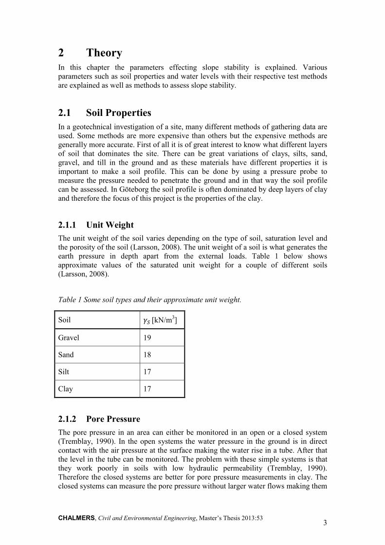
2.1.1 Unit Weight
The unit weight of the soil varies depending on the type of soil, saturation level and the porosity of the soil (Larsson, 2008). The unit weight of a soil is what generates the earth pressure in depth apart from the external loads. Table 1 below shows approximate values of the saturated unit weight for a couple of different soils (Larsson, 2008).
Table 1 Some soil types and their approximate unit weight.
Soil �� [kN/m3]
Gravel 19
Sand 18
Silt 17
Clay 17
2.1.2 Pore Pressure
The pore pressure in an area can either be monitored in an open or a closed system (Tremblay, 1990). In the open systems the water pressure in the ground is in direct contact with the air pressure at the surface making the water rise in a tube. After that the level in the tube can be monitored. The problem with these simple systems is that they work poorly in soils with low hydraulic permeability (Tremblay, 1990). Therefore the closed systems are better for pore pressure measurements in clay. The closed systems can measure the pore pressure without larger water flows making them

CHALMERS, Civil and Environmental Engineering, Master’s Thesis 2013:53 4
useful in soils like clay. The closed systems can monitor the pore pressure with fast variations and can also be set to automatic registrations of the pore pressure.
The pore pressure measurements taken in the area around Stora Hamnkanalen are all made with closed systems. Electrical probes are driven into the soil in a number of places that register the pore pressure periodically over a long time. Through this method it is established that the pore pressure is hydrostatical in the study area.
The pore pressure in the soil is a parameter that is needed for calculations regarding the clay. The total stresses in the soil are divided into effective stresses and the pore pressure. That way the pore pressure is subtracted from the total stress to get the effective stresses, see equation (1), which are commonly used to assess the behaviour of clays. A high pore pressure will act as a lifting force making the soil more stable to settlements (Sällfors, 2009).
�� = ��� + � (1)
In equation (1) the total stresses are denoted by ��, the effective stresses by ��� and the pore pressure by �.
2.1.3 Liquid Limit
The liquid limit of the soil sample is the point when the soil goes from a plastic behaviour to a liquid behaviour. The method to investigate the liquid limit uses the same rig as that for the fall cone test. A cone with the mass of 60 g and a point angle of 60° is dropped into the stirred sample and the penetration is measured. The liquid limit is obtained from the amount of water in the stirred sample resulting in a 10 mm penetration (Larsson, 2008).
2.1.4 Shear Strength
The shear strength of a soil is the ability to withstand changes in shape from different sorts of stresses (Sällfors, 2009). The shear strength is generally increasing linearly with the depth of the soil and is therefore easy to put into calculations of different sorts.
When assessing the shear strength of a cohesive soil, such as clays and some silts, it is important to consider if the conditions suggest a drained or an undrained analysis. The drained condition requires that the loading or the deformation is of such a slow character that no pore pressure develops during the process. In Sweden the clays are mostly very soft with very low hydraulic conductivity. Therefore for the analyses regarding ultimate limit state, where the analysed construction should not fail from the largest design load, an undrained condition is commonly used. As a slope stability analysis is an ultimate limit state analysis the undrained shear strength is used (Alén et al. 2012).

CHALMERS, Civil and Environmental Engineering, Master’s Thesis 2013:53 5
There are many different methods to evaluate the undrained shear strength, some can be executed in the field and some are in need of sophisticated laboratory equipment. The different methods give different values for the undrained shear strength and therefore a correction factor is needed in some cases to get closer to the actual shear strength.
2.1.4.1 Anisotropy
An anisotropic material has in comparison to isotropic material different properties in different directions and an example of such a material is often the clay in Göteborg. According to the Swedish Commission on Slope Stability, anisotropy calculations will always increase the calculated factor of safety for a slope. The anisotropy effects are larger if the slope is steep and if the liquid limitis low. As the slope investigated in this project is steep and the liquid limit is moderate, around 60 to 70 %, the anisotropic condition is of interest.
When considering anisotropy for a slope, the first step is to divide the slope into three zones. These three zones are the active shear zone, the direct shear zone and the passive shear zone, see Figure 1. The shear strength is considered to be different in the three zones. In the direct shear zone the value of � can be obtained from test such as direct shear tests, vane shear tests and fall cone tests corrected depending on the liquid limit. From the direct shear strength the active shear strength and the passive shear strength can be evaluated according to Table 2. For Table 2 a factor ��(��) is required and can be calculated according to equation (2) (Axelsson et.al, 1995). Also the angle of the slip surface, shown in Figure 2, is needed to estimate the active and passive shear strengths from Table 2. The angle � of the slip surface in Figure 2 is negative in the passive shear zone and positive in the active shear zone.
Figure 1 A = Active shear zone, B = Direct shear zone, C = Passive shear zone.
��(��) ≈ 0.31 × 0.71(�� − 0.2) (2)
A B C

CHALMERS, Civil and Environmental Engineering, Master’s Thesis 2013:53 6
Figure 2 Angle of the slip surface.
Table 2 Correction factors of the shear strength depending on the angle of the slip surface (Axelsson et.al, 1995).
� [°] �� �� !⁄ [-]
-30 ��(��) (0.25 + 0.75��(��))⁄
-20 (0.03 + 0.97��(��)) (0.25 + 0.75��(��))⁄
-10 (0.12 + 0.88��(��)) (0.25 + 0.75��(��))⁄
0 1
10 (0.41 + 0.59��(��)) (0.25 + 0.75��(��))⁄
20 (0.59 + 0.41��(��)) (0.25 + 0.75��(��))⁄
30 (0.75 + 0.25��(��)) (0.25 + 0.75��(��))⁄
40 (0.88 + 0.12��(��)) (0.25 + 0.75��(��))⁄
50 (0.97 + 0.03��(��)) (0.25 + 0.75��(��))⁄
60 1 (0.25 + 0.75��(��))⁄
2.2 Water Levels The Swedish Meteorological and Hydrological Institute henceforth referred to as SMHI has since the 1930’s conducted water level readings at different locations. In Göteborg SMHI has an observation station located in outer parts of the harbour area called Torshamnen. At this station hourly measurement of the water level has been
α1 α2

CHALMERS, Civil and Environmental Engineering, Master’s Thesis 2013:53 7
conducted since 1967. The water levels measured in Torshamnen are not exactly the same as in Stora Hamnkanalen, as it is located upstream. However the values from Torshamnen can in accordance to past water level investigations be recalculated to fit the situation in Stora Hamnkanalen (Göransson and Karlsson, 1996).
2.2.1 The Normal Distribution
The water levels in this project are interpreted as normally distributed. The water level can be seen as a random variable ' that has values between -∞ and ∞. The mean water level is denoted by ) and the standard deviation is denoted by �. The probability density function is expressed in equation (3) (Adams, 2006). In this case the equation returns the probability of a specific water level denoted by x.
*+,-(') = 1� × .' − )� / = 1
�√21 23(43+)56-5
(3)
The case specific mean water level ) is calculated through equation (4), where 789 is past observations of the water level.
) =:789;
<
9=> (4)
In order to express the standard deviation �, an expectation based on past observations denoted as ?(78) must be defined. The expectation of the water level is expressed in equation (5), where k is the number of observations of a corresponding water level 789.
?(78) =:789<
9=>× @9; (5)
The case specific standard deviation can now be expressed through equation (6) (Adams, 2006), where both ?(78) and ) is dependent on past observations.
� = A?(786) − )6 (6)
In cases where the probability of exceeding or underlying a specific water level is of interest, a cumulated expression of the general normal distribution can be used. In order to achieve a cumulated expression of the probability density function, *+,-(') is integrated above or beneath the investigated water level 78, see equation (7) (Adams, 2006).
B(') = 1�√21 × C 23(43+)
56-5
D�
3E
(7)
All normal distribution calculations in this project are made in the computer program Excel where these equations are pre-defined.

CHALMERS, Civil and Environmental Engineering, Master’s Thesis 2013:53 8
2.3 Soil Tests To obtain the data needed for an in depth investigation of a site a number of tests and measurements are needed. The two main groups of tests are disturbed and undisturbed tests. The disturbed tests can be performed in the field with certain equipment and the undisturbed tests are performed in a laboratory using undisturbed samples from the site. The undisturbed tests are in general more expensive than the disturbed tests but the data obtained is generally more detailed. The data used in this project comes from both sorts of test methods. The disturbed tests used are vane shear tests and cone penetration tests, and the undisturbed tests used are fall cone tests, direct shear tests and laboratory methods to investigate the liquid limit and the unit weight.
In slope stability analysis it is important to have good data on the shear strength. It is common to perform a number of different tests of the shear strength to be able to make a good evaluation. The different test of the undrained shear strength does not match each other and some tests are therefore altered to match the tests that are considered to be more real. The tests that need alteration are the vane shear tests and the fall cone tests. These tests are corrected with the same factor that can be obtained from the liquid limit. Equation (8) shows the factor that corrects the vane shear tests and the fall cone tests to match tests like direct shear tests and tri-axial shear tests (Axelsson et al, 1995).
) = (0.43 7�⁄ )�.FG ≥ 0.5 (8)
According to the Swedish Implementation Commission for the European Standards in Geotechnics, enough vane shear test shall be performed in the area to calibrate the cone penetration tests. This in order to get a good idea of the soils undrained properties in the area. After the alteration the tests can be plotted in one diagram and then the general shear strength can be evaluated. It is also important to have good knowledge of the site as properties may change drastically depending on the site. In the excavated channel, that was excavated a couple of centuries ago, the properties in the underlying soil are different from the properties that have not been excavated. Therefore tests were needed on both sides of the channel wall (Bengtsson et al. 2011).
2.4 Pile Properties The pile properties are calculated in accordance to the recommendations set by the Swedish Commission on Pile Research. For the strength class of the wood piles, class C30 is used with a surrounding relative humidity larger than 85% (Svahn and Alén, 2006).
The moment capacity MRd is calculated according to Eurocode 5, see equation (9), with the recommendations set by the Swedish Commission on Pile Research.
IJK = 7 × *LK (9)
The bending moment of inertia W is calculated with the condition of a circular cross section according to equation (10) (Lund, 2000).

CHALMERS, Civil and Environmental Engineering, Master’s Thesis 2013:53 9
7 = 1 × MN4
(10)
The design value fmd is calculated in accordance to Eurocode 5 where kmod varies with loading situation and relative humidity, fmk is dependent to the strength class of the wood and γM is determined by manufacturing conditions, see equation (11) (Al-Emrani et al, 2010).
*LK = @L K × *LO�P (11)
2.5 Slope Stability Model The stability of a slope or a cut is the result of the balance between the driving and opposing forces on each side. The driving forces are forces like soil masses and external loads and the opposing forces are external loads, water pressures and shear forces in the soil (Sällfors, 2009). The balance between these forces results in a factor of safety and the factor of safety can be calculated using a couple of different methods. The most common way to investigate the stability of a slope is to investigate the factor of safety of circular cylindrical slip surfaces. This way it is assumed that the failure of the slope will have a circular shape in the section of the slope.
2.5.1 Direct Method
One method to roughly estimate the stability of a slope is to use a method referred to as the direct method (Sällfors, 2009), were the driving forces are compared to a general shear resistance of the soil, see equation (12). This is a method that only estimate the stability but if a more accurate result of the stability is needed a more detailed methodology is necessary.
BQ = R� × �SK (12)
In equation (12), the factor of safety is denotedBQ, � is the general shear resistance, SK is the driving forces from external loads, earth loads and water pressures corrected with partial factors and R� is a geometrical parameter depending on the slope geometry.
To get a better value of the factor of safety the next step is to start to analyse individual slip surfaces. This can be done by hand calculations but it takes long time to calculate the amount of slip surfaces necessary. Therefore there are a number of computer programs that makes these calculations less time consuming.
2.5.2 Computer Aided Calculations
A more detailed method to calculate the stability of a slope is to use a computer program that divides the slope into a number of parts to get more correct values for

CHALMERS, Civil and Environmental Engineering, Master’s Thesis 2013:53 10
the shear strength on each part of the slope. As the shear strength normally vary with depth, these more sophisticated models take the variations of the shear strengths into account instead of using a mean value in the calculations. This methodology is used on each slip surface of the slope in order to find the most critical slip surface. This method is mostly used with the aid of computer software that can calculate multiple slip surfaces in a couple of seconds instead of spending hours trying to find the most critical slip surface by hand calculations. There are a couple of computer programs that can calculate the factor of safety for circular slip surfaces using these methods, for instance SLOPE and GeoSuite. When using these programs it is very important to have good data that can be put into the model and also make sure that the geometry of the slope is modelled correctly as it is a very important parameter.
When a model has been created in the program and the most critical slip surface is found it is also possible to add reinforcements to the model to investigate what improvements the reinforcements will result in. Reinforcements as piles, nails and anchors can be modelled in different ways and all the data for the reinforcements are added manually. Therefore it is important to have reliable data on the material parameters not only for the soils but also for the reinforcements. Such parameters could be the shear strength of the piles or the cohesion of the nails. It is also significant to note that the extra loading and disturbances during the installations of the reinforcements are not accounted for in the model.
2.5.2.1 SLOPE
The original shape of the program has been available on the general market since the late 1970's and is now used frequently in slope stability analysis. The models created in the program are based around five main components which are geometry, soil strength, pore-water pressure, reinforcements and imposed loading.
The program works in an iterative environment using a method of slices along a user defined number of slip surfaces and centres of rotation. The program divides the slip-body into slices and defines the forces acting on the created slice, see Figure 3. In this project the Morgenstern-Price method is used which takes both moment and force equilibrium of the slices into account. The intersected force- and moment factor of safety is in the end of the calculation procedure presented in the program (2010, GEO-SLOPE International Ltd.).

CHALMERS, Civil and Environmental Engineering, Master’s Thesis 2013:53 11
Figure 3 Overview of the common influential forces on the slices.
2.5.3 The Swedish Transport Administration
The governmental body that has ultimate responsibility for state-roads in Sweden is the Swedish Transport Administration. The technical requirements for improvements and new constructions to geo-constructions are expressed in the publication TK Geo 11. However in slope stability investigations the report Recommendations for Slope Stability Investigations by the Swedish Commission on Slope Stability can be used. TK Geo 11 defines constructions and their probability of failure in three safety classes. Safety class 1 is only applied in constructions where roads or railway is not involved. Safety class 2 is the most common for roads and applied if the subgrade does not include sensible clays. Safety class 3 is applied for railway constructions and if the subgrade includes sensible clays (Trafikverket, 2011).
2.5.4 Swedish Commission on Slope Stability
The Swedish Commission on Slope Stability was created in 1988 and its purpose is to initiate and coordinate research on slope stability, shear failure and methods to prevent failures. The report Recommendations for Slope Stability Investigations from 1995 covers the investigational methods and calculations needed to assess the stability of a slope. The purpose of this report is to increase and maintain the quality of slope stability investigations in Sweden. The purpose is also to make the investigations better without necessarily making them more expensive. The idea is that even if the investigations in some cases gets more expensive that may result in less expensive measures to the problem later on (Axelsson et al. 1995).
The report Recommendations for Slope Stability Investigations explains how to calculate many parameters regarding slope stability but the method used in this study is how to account for anisotropic conditions in the soil. The anisotropic conditions are important parameters in this study and therefore a solid method was needed for the calculations. The method used, which is established by the Swedish Commission on Slope Stability, is explained in chapter 3.3.1.1. The Swedish Commission on Slope

CHALMERS, Civil and Environmental Engineering, Master’s Thesis 2013:53 12
Stability recommends an Fc larger than 1.30 - 1.40 for existing slopes where the investigation can be described as detailed (Axelsson et al. 1995).
2.5.5 Swedish Commission on Pile Research
Although the specific withholding effects of piles in slope stability analysis are sparsely researched, there are however some researches on horizontally loaded piles available. The Swedish Commission on Pile Research has published several reports regarding the behaviour of piles and there surrounding soils in various boundary condition. In this thesis the method to estimate the maximum horizontal load Fxmax and maximum loading moment along the pile Mmax are calculated according to equation (13) and (14).
B4LT4 = (√2 − 1) × UV × 8 (13)
ILT4 = W 1√2 −12X × B4 × 8 (14)
Where L is the length of the pile and Uy is load applied from the soil as a reaction to the horizontal loading, which is calculated through equation (15).
UV = RQ × � (15)
Nc for clay is approximately 6 - 9 times the diameter of the piles, 6 is assumed in order to achieve conservative results. This method of calculations is only applicable when the pile itself can be viewed as short. The definition of a short pile is when the piles moment capacity is larger than the maximum loading moment, see equation (16) and when the capacity of the soil is fully utilized (Svahn and Alén, 2006).
ILT4 ≤ IJK (16)
2.5.5.1 Group Effect
When assessing the soil reaction due to a horizontal loading the group effect of the piles have to be considered. The maximum horizontal load Fxmax is not only dependent to the expression in equation (13). If the piles are placed close together perpendicular to the horizontal load the overall horizontal capacity is interpolated linearly between the cu and the Uy, the piles can be viewed as close if the distance between them is smaller than 2 diameters (Svahn and Alén, 2006).

CHALMERS, Civil and Environmental Engineering, Master’s Thesis 2013:53 13
3 Site Description The section investigated in this project is located in central Göteborg at Norra Hamngatan, see Figure 4. The area of interest is an overlying street situated next to a channel Stora Hamnkanalen with an intermediate channel wall constructed in the early 1600’s (Johansson, 2012). Since the channel wall is an old construction, the actual design of the underlying construction is surrounded by much uncertainty. Norra Hamngatan is a street daily used by public transport bus lines. The integrity of the channel and nearby constructions is of great importance not only because of public transportation but also because of cultural heritage and tourism.
Figure 4 Overview of the location of the investigated area (SGU, 2013).
3.1 Previous Stability Investigations The area of Stora Hamnkanalen has been subjected for investigations of the stability before; these previous investigations have been made by SWECO Infrastructure and Norconsult. These investigations have given some general inputs to this project, such as data that goes in to the model and the geometry of the channel area.
3.1.1 Detailed Stability Investigation, SWECO Infrastructure
The Detailed Stability Investigation was ordered by the City Planning Office of Göteborg to investigate the stability of pre-constructed areas in the city. This study is divided into three major parts. The part used for this project is sub area S302, Stora Hamnkanalen, of the investigation regarding southern Göteborg (Högsta, 2011). The information from the stability report made by SWECO Infrastructure that has been used as input data for this study is mainly the assumed water level variations in the
Investigated section
500 m
N

CHALMERS, Civil and Environmental Engineering, Master’s Thesis 2013:53 14
channel. These values have then been used to predict the variations from normal distribution, see chapter 4.1.1.1, based on the data from SWECO Infrastructure.
3.1.2 Diving Inspection Hamnkanalen, FROG Marine Service
The diving inspection was made in 2011 and has been divided into three parts. The three parts are divided depending on the bridges crossing the channel and the only stretch that has been used in this study is the most eastern part, closest to Fontänbron (Nyvall, 2011). In the diving inspection of Stora Hamnkanalen some important data regarding the piles have been presented. The data used from this diving inspection is the pile spacing of the outer row of piles underneath the channel wall. The spacing is an important parameter for calculations of the reacting forces from the piles, presented in chapter 3.3.2.
3.1.3 Stability Investigation, Norconsult AB
The purpose of Norconsult’s report was to investigate the slope stability of both channel walls in Stora Hamnkanalen. As this report was written after the detailed stability investigation, made by SWECO Infrastructure, some of the data in the report was taken from there (Johansson, 2012). The data used in this project taken from Norconsult’s report was mainly the shear strength of the soil and the stability model. The same data for the shear strengths has been used and the model used in SLOPE has been altered to match the purpose of this study. The data regarding the soil properties have been provided by ÅF AB and evaluated by Norconsult AB and can be seen in chapter 3.3.1. The model used to calculate the factor of safety in SLOPE can be seen in Appendix 1.
3.1.4 Parameters Stora Hamnkanalen, ÅF AB
This data is presented as a spread sheet in Excel, showing all the data from the performed ground investigations made by ÅF AB. The data file contains many different sorts of data but one part used in this study is the values of the liquid limit to calculate the anisotropic effects of the soil, show in chapter 3.3.1.1. Also the data of the shear strength that was taken from Norconsult’s report comes from these investigations. Therefore the data of the shear strength comes from ÅF AB indirectly.
3.2 Previous Proposed Measures As the previous investigations have shown that the stability is low some measures to prevent failure have been suggested. There are two suggested methods to increase the stability. The first measure is to reduce the driving forces of the slope and the second is to increase the opposing forces. The proposed way to decrease the driving forces is to excavate a part under the road and fill it with a material with lower density than the fill and clay. There are a number of materials that can be used for this kind of measure and the suggested materials are cellular plastic materials or light clinker. The second proposed measure is to increase the loads on the opposing side by adding additional fill in the channel. Also a combination of these two measures has been suggested as
CHALMERS, Civil and Environmental Engineering, Master’s Thesis 2013:53 15
the best way to increase the stability but there are also problems and complications connected to the improvements (Johansson, 2012).
The problems connected to the first measure is that during the installation of the lighter materials traffic needs to be redirected to another street as well as there might be some piping in the ground that needs to be moved. Another problem with the lighter materials is that they are vulnerable to high water levels due to uplift from the water in the soil. The light materials are lighter than water and will therefore create stresses in the soils with an upward direction that could cause problems. The solution with the additional fill in the channel is also connected to problems. The first problem is that during low water levels the additional fill will be visible and therefore less appealing. Also the fill may increase the risk of injuries of people falling into the channel during low water levels (Johansson, 2012).
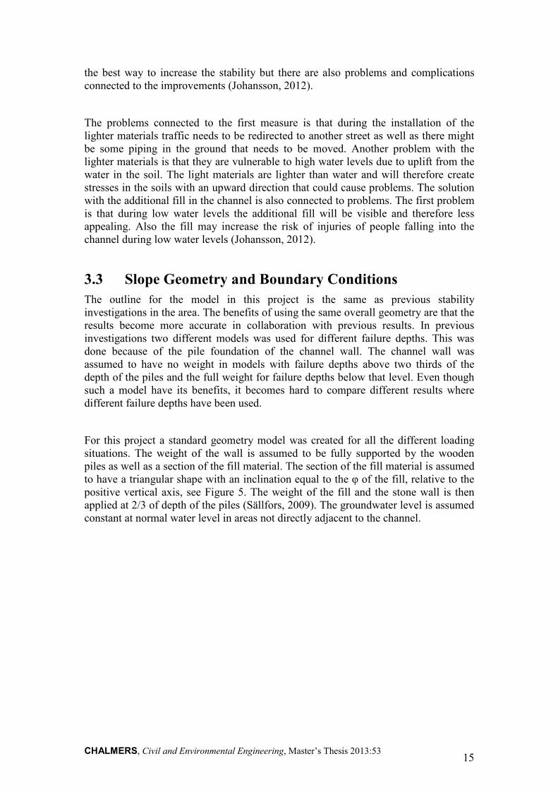
3.3 Slope Geometry and Boundary Conditions The outline for the model in this project is the same as previous stability investigations in the area. The benefits of using the same overall geometry are that the results become more accurate in collaboration with previous results. In previous investigations two different models was used for different failure depths. This was done because of the pile foundation of the channel wall. The channel wall was assumed to have no weight in models with failure depths above two thirds of the depth of the piles and the full weight for failure depths below that level. Even though such a model have its benefits, it becomes hard to compare different results where different failure depths have been used.
For this project a standard geometry model was created for all the different loading situations. The weight of the wall is assumed to be fully supported by the wooden piles as well as a section of the fill material. The section of the fill material is assumed to have a triangular shape with an inclination equal to the φ of the fill, relative to the positive vertical axis, see Figure 5. The weight of the fill and the stone wall is then applied at 2/3 of depth of the piles (Sällfors, 2009). The groundwater level is assumed constant at normal water level in areas not directly adjacent to the channel.

CHALMERS, Civil and Environmental Engineering, Master’s Thesis 2013:53 16
Figure 5 Principle of vertical pile load from wall and soil.
3.3.1 Soil Properties
The soil profile of the slope studied in this project is dominated by four major soil types. The street Norra Hamngatan lies on a fill layer with a thickness of approximately two meters. Under the fill material lays a clay layer with varying thickness, followed by a layer of friction material with a thickness of one meter with underlying bedrock. The soil profile under the channel Stora Hamnkanalen is similar to that of Norra Hamngatan but lacks the fill layer. The properties of the different material types in the slope section are presented in Table 3 (Johansson, 2012).
Table 3 Different material types and their properties (z1 ≤ 10 m, z2 ≤ 8 m).
Material type � [kN/m2] �� [kN/m3] �Z [kN/m3] [ [°]
Fill - 20 18 35
Clay (Norra Hamngatan) 14.5 + 1 × \1 16 16 -
Clay (Stora Hamnkanalen) 10.5 + 1.3 × \2 16 16 -
Friction material - 20 12 35
3.3.1.1 Increased Shear Strength Due To Anisotropic Conditions
The shear strength of the soil in the slope has been adjusted according to the method described in section 2.1.4.1 and the results are presented in this chapter. The first calculation was to calculate the value of ��(��) according to equation (2). To be able to do that a mean value of the liquid limit for was used and a value for ��(��) was
B]T^^
2 × 83
8
[

CHALMERS, Civil and Environmental Engineering, Master’s Thesis 2013:53 17
calculated for both the soil in the channel and the soil in the street. The calculated values of ��(��) and the liquid limits are presented in Table 4.
Table 4 Values of �0(R_) depending on the mean liquid limit.
�� [%] ��(��) [-] Stora Hamnkanalen 68.5 0.654
Norra Hamngatan 69.3 0.660
From ��(��) the correction factor�� �� !⁄ , shown in Table 5, was calculated for two different angles that were chosen to represent the active and the passive sides of the slip surface. The passive side was adjusted with the angle -20° and the active side was adjusted with the angle 30°, see appendix 4. The resulting correction factors are show in Table 5. The direct zone is not adjusted as the vane shear tests made in the area are adjusted to represent the direct shear zone.
Table 5 Correction factors for the passive and active zones.
� [°] �� �� !⁄ [-]
Passive zone -20 0.897
Active zone 30 1.228
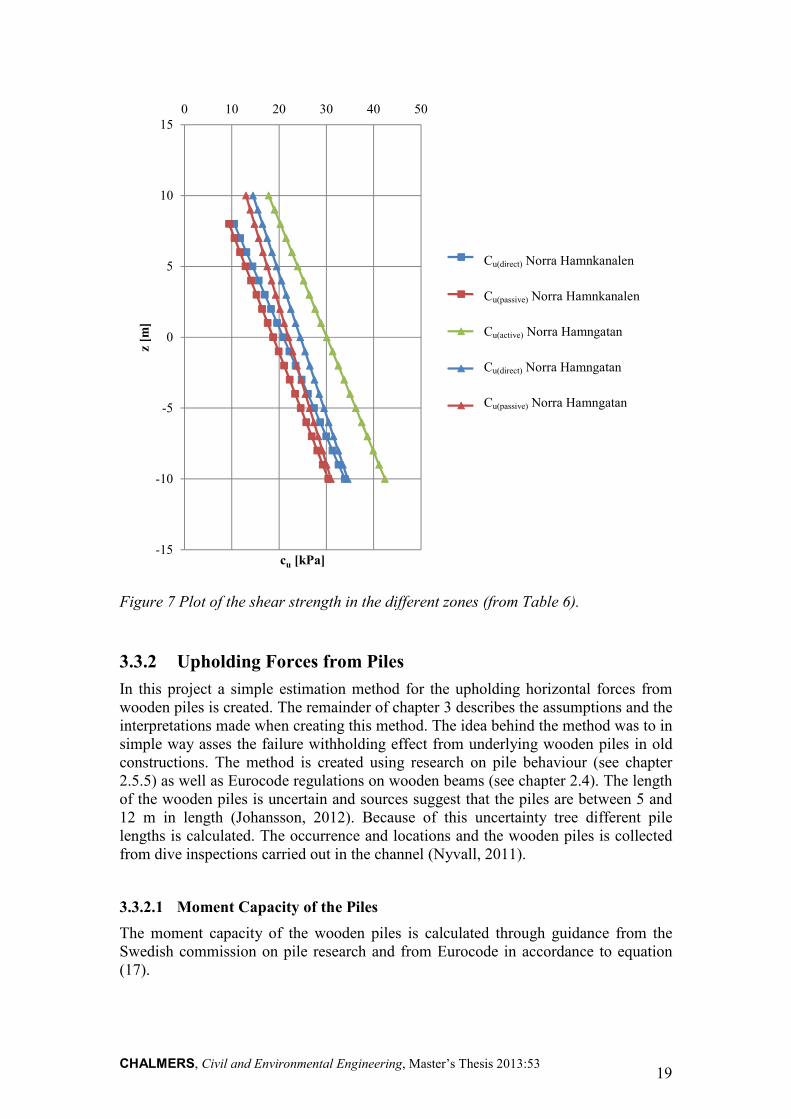
The direct zone is presumed to be stretched 15 degrees to each side of the vertical radius of the slip surface, see Figure 6. Therefore a part of the soil beneath the street may end up in the passive zone. Thus an adjusted value of the shear strength in that soil is needed for both the passive and the active zone. The soil in the channel will not be in the active zone due to the geometry of the slope and have therefore only been adjusted to the passive zone. The adjusted shear strength for the two types of soil is shown in Table 6 and Figure 7.

CHALMERS, Civil and Environmental Engineering, Master’s Thesis 2013:53 18
Table 6 Calculated shear strengths for the different zones (z1 ≤ 10 m, z2 ≤ 8 m).
Stora Hamnkanalen [kPa] Norra Hamngatan [kPa]
Passive zone 9.42 + 1.17\2 13.01 + 0.88\1
Direct zone 10.5 + 1.3\2 14.5 + \1
Active zone - 17.81 + 1.23\1
Figure 6 Principle for zone extent determination where `' = M × ab; �.
α α
Δx Δx
M
CHALMERS, Civil and Environmental Engineering, Master’s Thesis 2013:53 19
Figure 7 Plot of the shear strength in the different zones (from Table 6).
3.3.2 Upholding Forces from Piles
In this project a simple estimation method for the upholding horizontal forces from wooden piles is created. The remainder of chapter 3 describes the assumptions and the interpretations made when creating this method. The idea behind the method was to in simple way asses the failure withholding effect from underlying wooden piles in old constructions. The method is created using research on pile behaviour (see chapter 2.5.5) as well as Eurocode regulations on wooden beams (see chapter 2.4). The length of the wooden piles is uncertain and sources suggest that the piles are between 5 and 12 m in length (Johansson, 2012). Because of this uncertainty tree different pile lengths is calculated. The occurrence and locations and the wooden piles is collected from dive inspections carried out in the channel (Nyvall, 2011).
3.3.2.1 Moment Capacity of the Piles
The moment capacity of the wooden piles is calculated through guidance from the Swedish commission on pile research and from Eurocode in accordance to equation (17).
-15
-10
-5
0
5
10
150 10 20 30 40 50
z [m
]
cu [kPa]
Cu(direct) channel
Cu(passive) channel
Cu(active) NHamngatan
Cu(direct) NHamngatan
Cu(passive) NHamngatan
Cu(direct) Norra Hamnkanalen
Cu(passive) Norra Hamnkanalen
Cu(active) Norra Hamngatan
Cu(direct) Norra Hamngatan
Cu(passive) Norra Hamngatan
CHALMERS, Civil and Environmental Engineering, Master’s Thesis 2013:53 20
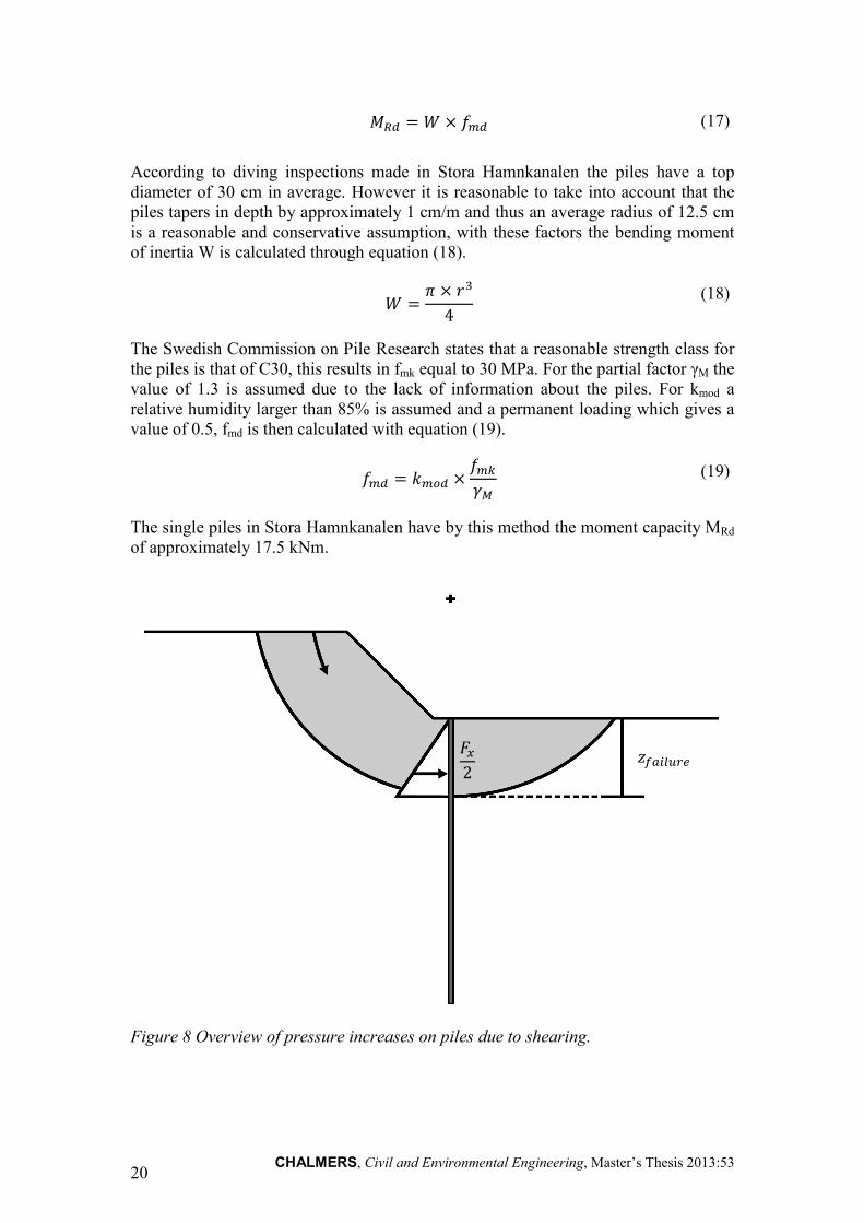
IJK = 7 × *LK (17)
According to diving inspections made in Stora Hamnkanalen the piles have a top diameter of 30 cm in average. However it is reasonable to take into account that the piles tapers in depth by approximately 1 cm/m and thus an average radius of 12.5 cm is a reasonable and conservative assumption, with these factors the bending moment of inertia W is calculated through equation (18).
7 = 1 × MN4
(18)
The Swedish Commission on Pile Research states that a reasonable strength class for the piles is that of C30, this results in fmk equal to 30 MPa. For the partial factor γM the value of 1.3 is assumed due to the lack of information about the piles. For kmod a relative humidity larger than 85% is assumed and a permanent loading which gives a value of 0.5, fmd is then calculated with equation (19).
*LK = @L K × *LO�P (19)
The single piles in Stora Hamnkanalen have by this method the moment capacity MRd of approximately 17.5 kNm.
Figure 8 Overview of pressure increases on piles due to shearing.
\eT9^�!fB42

CHALMERS, Civil and Environmental Engineering, Master’s Thesis 2013:53 21
3.3.2.2 Maximum Horizontal Load
There are two basic conditions that determine the size of the horizontal load the piles can mobilize. The first is dependent on the MRd of the piles while the other is dependent on the Uy of the soil. The calculations are based on methods presented by the Swedish Commission on Pile Research which has been adapted to fit landslide calculations, note that these adaptations are rough estimations of the actual conditions. The active shear side is assumed to produce an increase in pressure on the piles. This pressure is counteracted by a withholding force from the piles, see Figure 8. The withholding force from the piles is assumed to be a triangular distributed load within the shear body which has the largest value Fx, see Figure 9. The maximum bending moment along the pile therefore gets an addition from the moment generated within the shear body. The moment within the shear body is calculated through equation (20).
Igh =B4 × 12 × \eT9^�!f × 1
3 × \eT9^�!f (20)
Figure 9 Principal forces on the piles.
The addition from the shear body to the maximum bending moment along the pile is then inserted into equation (14) in order to evaluate the maximum horizontal load in terms of moment capacity creating equation (21).
ILT4 = W 1√2 −12X × B4 × 8 + 1
6 × \eT9^�!f6 × B4 <=>
B4 = ILT4W 1√2 −
12X × 8 + 1
6 × \eT9^�!f6
(21)
8√2
8
UV
UV
B42

CHALMERS, Civil and Environmental Engineering, Master’s Thesis 2013:53 22
With the pre-condition of a moment capacity from equation (17) of the pile larger than the maximum moment, equation (22) is created in order to assess the maximum horizontal load Fxmax,M.
B4LT4,P = IJKW 1√2 −
12X × 8 + 1
6 × \eT9^�!f6 (22)
The second basic condition is calculated directly through equation (13) with direct linearization of the block strength dependent by the pile area and the free soil area in the section creating equation (23).
B4LT4,Z = l√2 − 1m × UV × 8 × no9^f + � × 8 × ng 9^ (23)
When the calculations of the two conditions are completed for the tree different pile lengths a comparison between the two conditions is performed where the lowest obtained Fx is chosen for different failure depths and pile lengths, see Figures 10, 11 and 12.
Figure 10 Obtained Fx values for different failure depths and 5 m pile.
0
10
20
30
40
50
60
70
80
0 1 2 3 4 5 6
Fx
[kN
/m]
zfailure [m]
Fxmax(MRd)/m
Fxmax(U)/m
Fxdim(MRd,U)/m

CHALMERS, Civil and Environmental Engineering, Master’s Thesis 2013:53 23
Figure 11 Obtained Fx values for different failure depths and 8 m pile.
Figure 12 Obtained Fx values for different failure depths and 12 m pile.
3.3.2.3 Multiple Pile Rows
In this project a single pile row was used for different pile lengths. There are some indications of multiple pile rows in the study area (Högsta, 2011). The Swedish commission on pile research suggest that for situations involving multiple pile rows the capacity for a single pile row is multiplied by the number of rows. However a reduction of the capacity by 25% should be applied if the rows can be expressed as close, the rows is viewed as close if the distance between the rows is less than 3 pile diameters (Svahn and Alén, 2006). In order to give an example of a situation of multiple pile rows the capacity of 8 m piles in 3 rows was calculated, see Figure 13. As an example it can be observed that 3 rows of piles in relation to 1 row would
0
10
20
30
40
50
60
70
80
90
100
0 2 4 6 8 10
Fx
[kN
/m]
zfailure [m]
Fxmax(MRd)/m
Fxmax(U)/m
Fxdim(MRd,U)/m
0
20
40
60
80
100
120
140
160
0 5 10 15
Fx
[kN
/m]
zfailure [m]
Fxmax(MRd)/m
Fxmax(U)/m
Fxdim(MRd,U)/m

CHALMERS, Civil and Environmental Engineering, Master’s Thesis 2013:53 24
increase Fx with 200 % when MRd is the designing parameter and 90 % when Fx is controlled by Uy.
Figure 13 Obtained Fx values for different failure depths and 3 rows of 8 m pile.
3.4 Decision Support for Measurements in Existing Slopes In this project a recently developed method for assessing the required safety for existing slopes was used. This approach was chosen in order to evaluate the relevance of the results produced in the probability model. The method used was developed with the precondition of the actual functionality of an existing slope. The method provides a factor of safety which can be low but still maintaining the same probability of failure as that of a new slope structure with a higher factor of safety. The method takes two general factors of uncertainty into account; these are the uncertainty surrounding knowledge of the boundary conditions like soil properties and geometry which is usually addressed as knowledge uncertainty. The other general factor of uncertainty is the genuine uncertainty surrounding conditions like water levels and loads such as traffic loads (Alén, 2012).
The method distinguishes two different factors of safety as inputs to the method. The first factor of safety is the calculated Fc designated as F1 and a normal case factor of safety F0. F0 is calculated through normal slope stability calculations with the most commonly occurring boundary conditions. This method results in a recommended safety factor F2 after reinforcements, depending on the input data and the pursued safety class (Alén, 2012).
0
100
200
300
400
500
600
700
800
0 2 4 6 8 10
Fx
[kN
/m]
zfailure [m]
Fxmax(MRd)/m
Fxmax(U)/m
Fxdim(MRd,U)/m

CHALMERS, Civil and Environmental Engineering, Master’s Thesis 2013:53 25
4 Probability Model This chapter describes the function of the probability model, the assumptions that have set the boundary conditions and presents the input data that goes into the model. These are just the data that goes into the model regarding the probability of each scenario already modelled in SLOPE, see chapter 2.5.2.1 and appendix 1.
The probability model has been made to investigate the probability of each scenario modelled in SLOPE. In order to investigate the probability for each event modelled in SLOPE a new model was established using a number of assumptions, presented in the following chapter. In Excel a probability tree was created and each event was symbolized by a branch in the tree. Each branch has got a factor of safety from SLOPE and a probability depending on the likelihood of the event. As each event has got a factor of safety and a probability, these values have been matched to normal distributions which have been plotted in chapter 5. To be able to observe how the factor of safety changes with increasing number of parameters taken into account the model was divided into five parts. The first part was made using only the water levels from previous investigations and the different load cases. For the fifth, and last, model the inputs were more detailed including water levels from new data series, load variations, anisotropic conditions and pile forces. The idea was to observe the changes of the factor of safety by using five parts going from the boundary conditions close to the old investigation towards a model closer to the reality. Table 7 shows the data used for the five parts of the probability model.
Table 7 The five parts of the model were √ means that the criterion is considered and X means that the criterion is not considered.
Part Old water levels
New water levels
Three load cases
Anisotropic conditions
Horizontal pile forces
1 √ X √ X X
2 X √ √ X X
3 X √ √ √ X
4 X √ √ X √
5 X √ √ √ √
4.1 Inputs and Assumptions In order to connect each event to a probability a number of assumptions were made. These assumptions set the boundary conditions of the model and where therefore affecting the results. This chapter describes the assumptions for the data used in the probability model. The three parameters that were connected to probabilities and put into the model were water level variations, traffic loads and pile forces.

CHALMERS, Civil and Environmental Engineering, Master’s Thesis 2013:53 26
4.1.1 Water Levels
As the investigated slope is located in a channel, the water level in the channel has an impact on the stability of the slope. The water in the channel is acting like an opposing force and the low water levels are of interest for slope stability.
4.1.1.1 Water Levels from Previous Investigations
For part 1 the water levels was taken from the previous investigations and the water levels used are presented below. The water levels from these investigations are shown in Table 8.
Table 8 Water levels from previous investigations (Johansson, 2012).
The water level of the channel is considered to be normally distributed in accordance to chapter 2.2.1. As the mean values are either for low or high water it is assumed that there is one distribution for each of the high and low waters. As the values for LLW and HHW are the minimum and maximum values over 50 years these values are set to represent the 2% percentile for the normal distribution around the mean values MHW and MLW. In order to find the number of standard deviations that represents the 2% percentile a table for the normal distributions are needed, presented in appendix 2 (Alén et al, 2012). There are however no value for the 98% confidence interval and thus a linear interpolation between the nearest confidential intervals was made. Table 9 shows the intervals and the number of standard deviations that corresponds to the percentiles as well as the interpolated value of the 98% confidence interval. After the interpolation is made the standard deviations for the two functions are obtained from the difference in water level between the extreme value and the mean value divided by the corresponding number of standard deviations.
Water level Level [m]
HHW +11.6
MHW +11.0
NW +10.1
MLW +9.4
LLW +8.9

CHALMERS, Civil and Environmental Engineering, Master’s Thesis 2013:53 27
Table 9 Confidence intervals and the corresponding number of standard deviations (Alén et.al, 2012).
Confidence Interval [%] No of Standard Deviations [-]
97.98 2.05
98.03 2.06
98 2.054
Thereafter the mean value and the standard deviation, displayed in Table 10, can be used to plot the normal distributions. Figure 14 shows the probability density functions for the two distributions of low and high water levels plotted in Excel.
Table 10 Mean and standard deviation for both water levels.
Water level Mean [m] Standard Deviation [m]
HW +11 0.29211
LW +9,4 0.24343
Figure 14 Normal distributions showing the low water in blue and the high water in red.
In Figure 14 it can be seen that the normal water, which is +10.1 meter, is located in the intersection of the two distributions meaning that the normal water level is neither high water nor low water. The low water levels will affect the stability of the slope in
0
0,2
0,4
0,6
0,8
1
1,2
1,4
1,6
1,8
8,5 9 9,5 10 10,5 11 11,5
Den
sity
[-]
Water level [m]
LW
HW

CHALMERS, Civil and Environmental Engineering, Master’s Thesis 2013:53 28
a negative way, in comparison to the high water levels which in this case can be seen as preferable, therefore the focus from now will be on the low water.
To continue the investigation with focus on the low water levels the plot was reduced to only include the low water. Figure 15 shows the normal distribution for the low water.
Figure 15 Normal distribution for low water levels.
In normal distributions plotted as in Figure 14 and 15 the probability is represented by the area below the plot. The mean value is represented by the peak of the plot and as the normal distribution is symmetric around the mean value it is a 50 % probability that the water level will be below the mean and 50 % that it will be above the mean. To be able to put the water levels into the model with a corresponding probability it is often better to use the cumulative function for the same normal distribution instead of the probability density function. In the cumulative function, shown in Figure 16, the probability is not represented by an area but instead a number displayed on the y-axis.
0
0,2
0,4
0,6
0,8
1
1,2
1,4
1,6
1,8
8,5 9 9,5 10 10,5
Den
sity
[-]
Water level [m]
LW

CHALMERS, Civil and Environmental Engineering, Master’s Thesis 2013:53 29
Figure 16 The cumulative function for the normal distribution of the low water levels.
In the cumulative function the density is represented by the inclination of the plot instead of on the y-axis as in the probability density function. From the cumulative function a number of water level intervals have been chosen where the middle value of the interval is representing the water level with a resulting probability. These water levels and probabilities can then be put into the model to cover the water level changes. The chosen intervals with the resulting probabilities and water levels are presented in Table 11.
Table 11 Water level intervals, resulting water levels and resulting probabilities from the cumulative function.
Water level interval [m] Resulting water level [m] Resulting probability [-]
LLW (< 8.9) +8.9 0.02
LW (8.9-9.3) +9.1 0.32
MLW (9.3-9.5) +9.4 0.32
HLW (9.5-9.9) +9.7 0.32
HHLW (> 9.9) +9.9 0.02
As the low water is measured as the lowest water level during a year, the investigation is then limited to that specific case. This means that the model will only be adapted to the event of a low water state.
0
0,2
0,4
0,6
0,8
1
1,2
8,5 9 9,5 10 10,5
Pro
bab
ilit
y [-
]
Water level [m]
LW

CHALMERS, Civil and Environmental Engineering, Master’s Thesis 2013:53 30
4.1.1.2 Water Levels from New Data Series
In order to investigate a more realistic case of the slope new data of the water levels were ordered from the SMHI. The data available for water levels in Göteborg are measured further out in the cities harbour at Torshamnen. As Stora Hamnkanalen is located upstream from Torshamnen the water levels from Torshamnen had to be recalculated corresponding to levels at Stora Hamnkanalen. The new measurements were also presented in the new height system RH2000, introduced 2013, and had to be converted to the old local system GH88, used for all the other heights in this investigation. The new data series is water level measurements taken each hour since 1967 (SMHI, 2013). The difference between Torshamnen and Stora Hamnkanalen is an increase of around 10 cm as Stora Hamnkanalen is located upstream (Göransson, 1996). After the addition of 10 cm and a conversion to the old height system the annual low waters were plotted from the data series. The low annual low water levels are presented in Figure 17.
Figure 17 Annual low water levels from new data series (SMHI, 2013).
From these annual low water levels a normal distribution was made to be able to connect the water levels used to a probability. In this case the same probabilities have been used as for the values from the previous investigations. The difference is then that each probability represents a different water level than before. Table 12 shows the new water levels and the corresponding probabilities.
9
9,1
9,2
9,3
9,4
9,5
9,6
9,7
9,8
1965 1975 1985 1995 2005 2015
Wat
er l
evel
[m
]
Year
Annual Low Waters

CHALMERS, Civil and Environmental Engineering, Master’s Thesis 2013:53 31
Table 12 The corresponding probabilities for the new water levels.
Water level [m] Resulting probability [-]
LLW (+9.29) 0.02
LW (+9.41) 0.32
MLW (+9.52) 0.32
HLW (+9.62) 0.32
HHLW (+9.74) 0.02
When both the new and the old normal distributions of the low water levels are plotted in the same diagram it shows that the previous case has a much wider spread, and will therefore have a higher probability of low levels. Figure 18 shows the cumulative normal distribution for both the new and old low water levels.
Figure 18 The cumulative normal distributions of the new and the old low water levels.
4.1.2 Traffic Loads
The traffic loads are loads that will lower the factor of safety of the slope as they are driving forces. There are three different traffic loads that have been put into the model, the maximum traffic load and the maximum pedestrian load according to the Swedish Traffic Administration (Trafikverket, 2011) as well as an unloaded case. For
0
0,2
0,4
0,6
0,8
1
1,2
8,7 9,2 9,7 10,2
Pro
bab
ilit
y [-
]
Water level [m]
Old min/year
New min/year

CHALMERS, Civil and Environmental Engineering, Master’s Thesis 2013:53 32
the loads to last long enough to lead to failure it was assumed that only busses, that stop for people to exit and enter the bus, can trigger that load case. Therefore the assumed hours of rush hour will be representing the maximum load, the hours in the middle of the night will be the no load case as the busses are not running and the rest of the time will represent the normal load case. The normal load case is represented by the maximum pedestrian load case. Each load case and the assumed durations are explained in Table 13. The three different load cases and their corresponding probabilities are presented in Table 14.
Table 13 Durations of the three different load cases.
Load Type Duration
Maximum Load Three hours during the morning and the afternoon, only on weekdays
Normal Load 13 hours during the weekdays, 19 hours during the weekends
No Load Five hours during the night, each night
Table 14 The three different load cases modelled.
Load Type Load [kPa] Probability [-]
Maximum Traffic Load 13 5/28
Maximum Pedestrian Load 5 103/168
No Load 0 5/24
4.1.3 Pile Forces
The horizontal pile forces assumed to act as reinforcements in the soil, described in chapter 3.3.2, have also been connected to uncertainties. In the probability tree the pile forces were added last and have got three branches. Each branch represents a case with varying amount of horizontal force that strengthens the soil. The forces vary with depth and depending on the radius of the slip surface the applied forces varies throughout the probability tree. For each branch in the model the piles have a different length and therefore a different resulting force. As the piles are believed to be between 5 and 12 meters a triangular distribution of the pile lengths was used to assess the probability of the lengths. The pile lengths modelled are 5, 8 and 12 meters where 8 meters was considered to be the mean value of the pile length. Therefore a triangular distribution was made and evaluated; the triangular distribution is presented in Figure 19.

CHALMERS, Civil and Environmental Engineering, Master’s Thesis 2013:53 33
Figure 19 Triangular distribution of pile lengths.
The probability of pile lengths of 5 meters is represented by the area to the left of the line L1, the probability of pile lengths of 8 meters is represented by the area between lines L3 and L1 and the probability of piles of 12 meters is represented by the area to the right of line L3. The line L2 shows the peak of the distribution, which is the mean value. Table 15 presents the probabilities from Figure 19.
Table 15 Probabilities from the areas in Figure 20.
Pile length [m] Probability [-]
5 0.107
8 0.75
12 0.143
4.2 Resulting Probability Model The final probability model forms five probability trees with varying number of branches. Part 4 and 5 has in total 45 branches each with a factor of safety for the slope and a resulting probability for each branch. The probabilities and the factors of safety have then been plotted and matched to distributions and these results are presented in chapter 5. The entire final probability model can be seen in appendix 3. Figure 20 shows the top nine branches of part 4.
0
1
2
3
4
5
6
7
4 6 8 10 12
Den
sity
[-]
Pile length [m]
T-distribution
L1
L2
L3
Triangular distribution

CHALMERS, Civil and Environmental Engineering, Master’s Thesis 2013:53 34
Water level Traffic load Pile length Factor of safety
5m 15,22 kN 1,25
0,107 0,000382
13 kPa 8m 22,17 kN 1,22
0,178571 0,75 0,002679
12m 14,7 kN 1,16
0,143 0,000511
5m 16,3 kN 1,47
0,107 0,001312
LLW 9,29m 5 kPa 8m 23,93 kN 1,43
0,02 0,613095 0,75 0,009196
12m 15,93 kN 1,35
0,143 0,001753
5m 26,89 kN 1,61
0,107 0,000446
0 kPa 8m 38,38 kN 1,61
0,208333 0,75 0,003125
12m 28,26 kN 1,52
0,143 0,000596
Figure 20 The top nine branches of part 4.

CHALMERS, Civil and Environmental Engineering, Master’s Thesis 2013:53 35
5 Results This chapter presents the result from the five parts of the probability model. The results have been plotted as cumulative normal distributions matched to the results from the probability trees. These plots were then combined to view the differences depending on the boundary conditions explained in the previous chapter.
5.1 Resulting Plots from Probability Trees The result of the probability tree for each part was at first plotted as a scatter with the factor of safety on one axis and the accumulated probability on the other axis. These plots were then matched to cumulative normal distributions, which is based on a mean value and a standard deviation. That way the results can be compared and evaluated from the matching distributions. As the five parts were conducted individually without impact from one another they are also plotted separately. Figure 21 to 25 shows the results of part 1 to 5 and Figure 26 shows the resulting cumulative normal distributions for each part in one combined plot.
Figure 21 Resulting factors of safety and matching distribution for part 1.
0
0,2
0,4
0,6
0,8
1
1,2
0,9 1,1 1,3 1,5 1,7 1,9
Pro
bab
ilit
y [-
]
Factor of safety [-]
Part 1
Match

CHALMERS, Civil and Environmental Engineering, Master’s Thesis 2013:53 36
Figure 22 Resulting factors of safety and matching distribution for part 2.
Figure 23 Resulting factors of safety and matching distribution for part 3.
0
0,2
0,4
0,6
0,8
1
1,2
0,9 1,1 1,3 1,5 1,7 1,9
Pro
bab
ilit
y [-
]
Factor of safety [-]
Part 2
Match
0
0,2
0,4
0,6
0,8
1
1,2
0,9 1,1 1,3 1,5 1,7 1,9
Pro
bab
ilit
y [-
]
Factor of safety [-]
Part 3
Match

CHALMERS, Civil and Environmental Engineering, Master’s Thesis 2013:53 37
Figure 24 Resulting factors of safety and matching distribution for part 4.
Figure 25 Resulting factors of safety and matching distribution for part 5.
The first observation of the results is that the scattered values and the matching distributions seemed to be moving to the right as the numbers of considered parameters were increased. As the x-axis represents the factor of safety this means that the factor of safety was increased when the stabilizing factors were added. This can be seen in Figure 26, which shows the normal distributions for all the parts and in Table 16, which presents the mean value and the standard deviation for the five parts.
0
0,2
0,4
0,6
0,8
1
1,2
0,9 1,1 1,3 1,5 1,7 1,9
Pro
bab
ilit
y [-
]
Factor of safety [-]
Part 4
Match
0
0,2
0,4
0,6
0,8
1
1,2
0,9 1,1 1,3 1,5 1,7 1,9
Pro
bab
ilit
y [-
]
Factor of safety [-]
Part 5
Match

CHALMERS, Civil and Environmental Engineering, Master’s Thesis 2013:53 38
Figure 26 The combined cumulative normal distributions of parts 1 to 5.
Table 16 Mean values and standard deviations for the normal distributions.
Part Mean factor of safety [-] Standard deviation [-]
1 1.19 0.09
2 1.2 0.1
3 1.32 0.1
4 1.46 0.12
5 1.59 0.12
5.2 Results from Decision Support Methodology In addition to the probability trees, that take a number of supporting parameters into account, another probabilistic method was used to investigate the needed factor of safety of pre-constructed slopes after reinforcements. This method is described in chapter 3.4 and uses inputs from part 2. From the resulting probability tree of part 2 the values of F0 and F1 were taken. F1 is the factor of safety from the most critical water levels with the highest load and F0 is the factor of safety from the normal low water level and without load. In this case F1 was 1.05 and F0 1.34, (see appendix 3, part 2 F1 is equal to LLW(15 kPa) and F0 is equal to MLW(0 kPa)). These values have then been plotted according to the method and the resulting plots can be seen in Figure 27.
0
0,2
0,4
0,6
0,8
1
1,2
0,9 1,1 1,3 1,5 1,7 1,9
Pro
bab
ilit
y [-
]
Factor of safety [-]
Part 1
Part 2
Part 3
Part 4
Part 5

CHALMERS, Civil and Environmental Engineering, Master’s Thesis 2013:53 39
Figure 27 Schematic diagram of the sought-after factor of safety F2 (Alén, 2012).
The results of this method suggest that F2 should be around 1.3 after reinforcements have been added to the slope.
5.3 Evaluation of Results The results from the probability trees show that the mean factor of safety increases when more stabilising parameters are taken into account. They also show that the standard deviation of the normal distributions increase. Table 17 shows how the mean factor of safety and the standard deviation increased when the boundary conditions of the model was changed.
1 1.1 1.2 1.3 1.4 1.5 1.6 1.71
1.1
1.2
1.3
1.4
1.5
1.6
1.7
SK3SK2SK1SK0F2=F1
F1
F0 1.3=
1 1.1 1.2 1.3 1.4 1.5 1.6 1.71
1.1
1.2
1.3
1.4
1.5
1.6
1.7
SK3SK2SK1SK0F2=F1
F1
F2
F0 1.4=
Undrained
Safety class 3
Safety class 2
Safety class 1
Safety class 0
F2 = F1
F0 = 1.3
F1
F 2
Undrained
Safety class 3
Safety class 2
Safety class 1
Safety class 0
F2 = F1
F0 = 1.4
F1
F 2
CHALMERS, Civil and Environmental Engineering, Master’s Thesis 2013:53 40
Table 17 Increase in factor of safety and standard deviation in comparison to part 1.
Part Increase in factor of safety [-] / [%] Increase in standard deviation [-] / [%]
1 - / - - / -
2 0.01 / 0.8 % 0.01 / 11.1 %
3 0.13 / 10.9 % 0.01 / 11.1 %
4 0.27 / 22.7 % 0.03 / 33.3 %
5 0.40 / 33.6 % 0.03 / 33.3 %
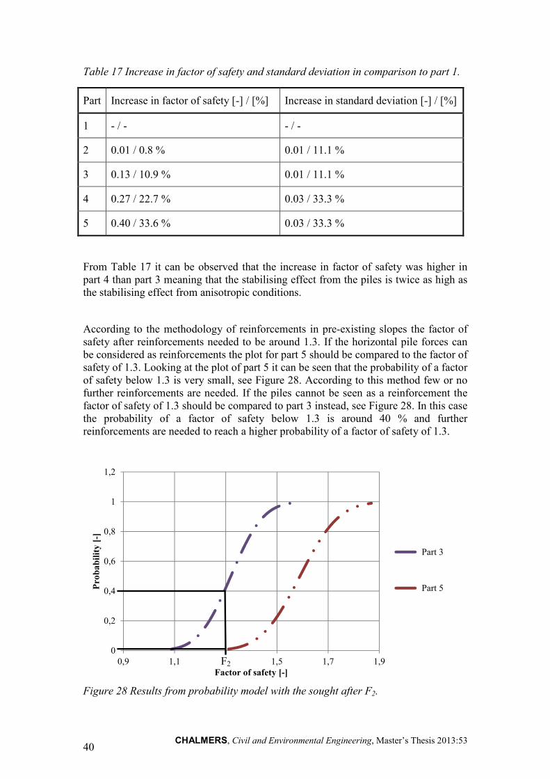
From Table 17 it can be observed that the increase in factor of safety was higher in part 4 than part 3 meaning that the stabilising effect from the piles is twice as high as the stabilising effect from anisotropic conditions.
According to the methodology of reinforcements in pre-existing slopes the factor of safety after reinforcements needed to be around 1.3. If the horizontal pile forces can be considered as reinforcements the plot for part 5 should be compared to the factor of safety of 1.3. Looking at the plot of part 5 it can be seen that the probability of a factor of safety below 1.3 is very small, see Figure 28. According to this method few or no further reinforcements are needed. If the piles cannot be seen as a reinforcement the factor of safety of 1.3 should be compared to part 3 instead, see Figure 28. In this case the probability of a factor of safety below 1.3 is around 40 % and further reinforcements are needed to reach a higher probability of a factor of safety of 1.3.
Figure 28 Results from probability model with the sought after F2.
0
0,2
0,4
0,6
0,8
1
1,2
0,9 1,1 1,3 1,5 1,7 1,9
Pro
bab
ilit
y [-
]
Factor of safety [-]
Part 3
Part 5
F2

CHALMERS, Civil and Environmental Engineering, Master’s Thesis 2013:53 41
6 Discussion In this chapter the assumptions and the uncertain parameters that affect the calculations have been discussed. These parameters have been discussed to give our perspective on how the uncertainties affect the results. Also the results and the variations of the results are discussed in this chapter.
6.1 Model The model that has been used is based on the geometric properties of the site. The geometry used is the same as in the previous investigations and we believe that the geometric conditions are correct. However the geometry was taken from one single section of the slope. As the stretch is around 140 meters long, investigating another section may change the geometry and therefore the results. It is hard to estimate to which extent the geometry change the results as it is one parameter that has remained unchanged throughout the project. The section used is the one where we had the most data and it is also a section with deep layers of clay. In order to reduce the amount of slip surfaces calculated the focus has been on the most critical slip surface for each individual load case. The benefit of using this methodology is that it is easy to compare the results for each slip surface and also easy to display. The negative thing about this methodology is that the slip surface may change when the boundary conditions such as pile forces are added. But as the slip surfaces have been locked at the most critical cases, these eventual changes are not considered. The reason why we decided to lock the slip surface was that we were interested in looking at how the stability increased for one specific case when the pile forces and anisotropic conditions were added.
As the final model is in the form of five probability trees with various amounts of branches, there may be reasons to believe that the number of individual cases is too few. More branches in the probability trees would probably improve the results but as we are quite happy with the pattern of the results we believe that the actual distributions of the results would not have changed significantly due to a larger model. One more level of data that could have been put into the model is the 3D effects on the slope. However we did not find any good method to estimate the 3D effects and put them into the SLOPE model. The 3D effects will work as a stabilising factor and therefore increase the stability. Excluding the 3D effects have therefore generate a more conservative model.
6.2 Input Data The calculations of the slope stability are the most central part of the study. If the parameters that are used in the model are uncertain it will also influence the results. It is important to separate the sorts of uncertainties that have been used. The uncertainties that have been used in the model are distributions of some of the parameters but there are also uncertainties connected to whether the assumptions are correct or not.

CHALMERS, Civil and Environmental Engineering, Master’s Thesis 2013:53 42
6.2.1 Water Levels
As described in previous chapters two different water level assumptions have been made. First the old data from the previous investigations were used and a distribution of the water level was calculated. However, we had reason to believe that the values of the water level from that data were incorrect so we decided to order data from SMHI to see if this assumption was correct. The new data series from SMHI showed that that water levels were not distributed as believed in the previous investigations. Therefore we decided to use the water levels obtained from SMHI because SMHI can be considered as a reliable source. The new water level variations are therefore considered to be quite certain as the data series stretches back to 1967 and we believe that the measurements of the data is of good quality. As the data from SMHI have been measured every hour the assumptions regarding the water levels also include that the modelled water levels last for one hour.
6.2.2 Soil Parameters
The soil parameters used in the model were taken from the previous investigations and we believe that the shear strength of the soil has been evaluated properly. The data on the liquid limit was also taken from the soil investigations and seemed reasonable with low variations. No uncertainty parameters were added to the soil properties for the slope stability calculations. The reason for this is that there is no good way of adding uncertainties in SLOPE. Adding uncertainties would require multiple SLOPE calculations for each branch of the probability tree. This would also require some kind of distribution of the shear strength of the soil. The soil parameters are of great importance when assessing the stability but we believe that the uncertainty and variation of the soil parameters are much smaller than for the other assumptions and were therefore discarded.
6.2.3 Traffic Loads
The traffic loads used in the model are the same values as in the recommendations from the Swedish Transport Administration in TK Geo 11. The loads used in this recommendation are very large and we believe that the largest loads are very unlikely. Therefore three different load cases were used as we assumed that the road is not subjected to loads as large as recommended at all times. We assumed that the largest load only could be applied by fully loaded busses and that these busses only are arriving at a few hours each day. These large loads are considered to be highly unlikely but as the duration of the water levels are considered to be one hour long the probability of the traffic load need to be modelled on an hourly basis as well. To model the traffic loads we had to figure out the probability of each load case depending on the duration of the water levels. The fact that the loads are believed to be too large is not taken into account in the model in any other way than that the probability of the large load case is smaller than the other cases. This could have been modelled using a probability distribution were the mean value is offset from the centre. But to get a good coverage of such a distribution more load inputs would have been needed and these values would all be based on assumptions which would make the whole model much more uncertain. Also it would be hard to connect the traffic loads to the water levels lasting for one hour. We therefore decided to estimate the same traffic loads as suggested in TK Geo 11 along with an unloaded case connected
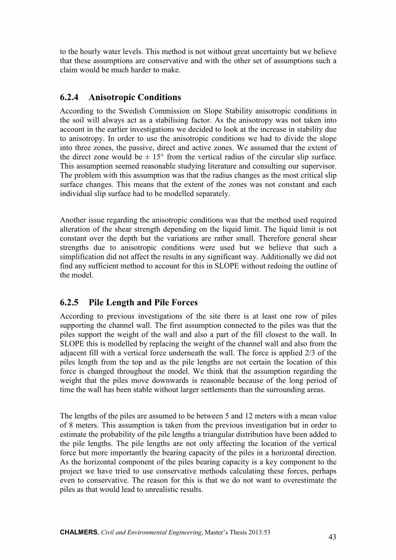
CHALMERS, Civil and Environmental Engineering, Master’s Thesis 2013:53 43
to the hourly water levels. This method is not without great uncertainty but we believe that these assumptions are conservative and with the other set of assumptions such a claim would be much harder to make.
6.2.4 Anisotropic Conditions
According to the Swedish Commission on Slope Stability anisotropic conditions in the soil will always act as a stabilising factor. As the anisotropy was not taken into account in the earlier investigations we decided to look at the increase in stability due to anisotropy. In order to use the anisotropic conditions we had to divide the slope into three zones, the passive, direct and active zones. We assumed that the extent of the direct zone would be ± 15° from the vertical radius of the circular slip surface. This assumption seemed reasonable studying literature and consulting our supervisor. The problem with this assumption was that the radius changes as the most critical slip surface changes. This means that the extent of the zones was not constant and each individual slip surface had to be modelled separately.
Another issue regarding the anisotropic conditions was that the method used required alteration of the shear strength depending on the liquid limit. The liquid limit is not constant over the depth but the variations are rather small. Therefore general shear strengths due to anisotropic conditions were used but we believe that such a simplification did not affect the results in any significant way. Additionally we did not find any sufficient method to account for this in SLOPE without redoing the outline of the model.
6.2.5 Pile Length and Pile Forces
According to previous investigations of the site there is at least one row of piles supporting the channel wall. The first assumption connected to the piles was that the piles support the weight of the wall and also a part of the fill closest to the wall. In SLOPE this is modelled by replacing the weight of the channel wall and also from the adjacent fill with a vertical force underneath the wall. The force is applied 2/3 of the piles length from the top and as the pile lengths are not certain the location of this force is changed throughout the model. We think that the assumption regarding the weight that the piles move downwards is reasonable because of the long period of time the wall has been stable without larger settlements than the surrounding areas.
The lengths of the piles are assumed to be between 5 and 12 meters with a mean value of 8 meters. This assumption is taken from the previous investigation but in order to estimate the probability of the pile lengths a triangular distribution have been added to the pile lengths. The pile lengths are not only affecting the location of the vertical force but more importantly the bearing capacity of the piles in a horizontal direction. As the horizontal component of the piles bearing capacity is a key component to the project we have tried to use conservative methods calculating these forces, perhaps even to conservative. The reason for this is that we do not want to overestimate the piles as that would lead to unrealistic results.
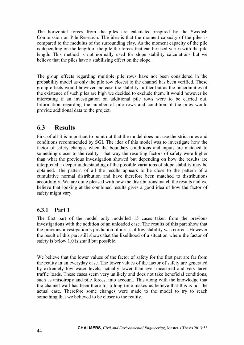
CHALMERS, Civil and Environmental Engineering, Master’s Thesis 2013:53 44
The horizontal forces from the piles are calculated inspired by the Swedish Commission on Pile Research. The idea is that the moment capacity of the piles is compared to the modulus of the surrounding clay. As the moment capacity of the pile is depending on the length of the pile the forces that can be used varies with the pile length. This method is not normally used for slope stability calculations but we believe that the piles have a stabilising effect on the slope.
The group effects regarding multiple pile rows have not been considered in the probability model as only the pile row closest to the channel has been verified. These group effects would however increase the stability further but as the uncertainties of the existence of such piles are high we decided to exclude them. It would however be interesting if an investigation on additional pile rows were to be carried out. Information regarding the number of pile rows and condition of the piles would provide additional data to the project.
6.3 Results First of all it is important to point out that the model does not use the strict rules and conditions recommended by SGI. The idea of this model was to investigate how the factor of safety changes when the boundary conditions and inputs are matched to something closer to the reality. That way the resulting factors of safety were higher than what the previous investigation showed but depending on how the results are interpreted a deeper understanding of the possible variations of slope stability may be obtained. The pattern of all the results appears to be close to the pattern of a cumulative normal distribution and have therefore been matched to distributions accordingly. We are quite pleased with how the distributions match the results and we believe that looking at the combined results gives a good idea of how the factor of safety might vary.
6.3.1 Part 1
The first part of the model only modelled 15 cases taken from the previous investigations with the addition of an unloaded case. The results of this part show that the previous investigation’s prediction of a risk of low stability was correct. However the result of this part still shows that the likelihood of a situation where the factor of safety is below 1.0 is small but possible.
We believe that the lower values of the factor of safety for the first part are far from the reality in an everyday case. The lower values of the factor of safety are generated by extremely low water levels, actually lower than ever measured and very large traffic loads. These cases seem very unlikely and does not take beneficial conditions, such as anisotropy and pile forces, into account. This along with the knowledge that the channel wall has been there for a long time makes us believe that this is not the actual case. Therefore some changes were made to the model to try to reach something that we believed to be closer to the reality.

CHALMERS, Civil and Environmental Engineering, Master’s Thesis 2013:53 45
6.3.2 Part 2
The second part of the model is similar to the first part and the only difference is that the water levels used are the low water levels from the new data series instead of the previous assumptions. As the boundary conditions are similar to part 1, the results are also similar. The same interpretation of the results of part 1 applies for part 2 as no beneficial factors are used here either. But as the water levels used are more reliable, we believe part 2 is somewhat closer to the real case but still far from the truth regarding the stability as the stability still is very low.
6.3.3 Part 3
For part 3 the same water levels as in part 2 are used but with the addition of anisotropic conditions of the soil. The addition of anisotropy raises the stability considerably which was expected according to the Swedish Commission on Slope Stability. The mean factor of safety has increased from 1.2 to 1.32, an increase of 10%, when adding the anisotropic conditions to the model. The increase is not just for the mean value but there is an offset for most of the distribution. As the results are considered to be normally distributed the offset cannot be applied to the whole distribution as the lower and upper parts are levelling off. According to the Swedish Commission on Slope Stability anisotropic conditions can be applied to a slope stability analysis and we believe that the stability obtained from part 3 may be an explanation to why there are no indications of failure.
6.3.4 Part 4
For both part 4 and 5 the pile forces were added to show how a horizontal force from the piles would affect the stability. We thought that it could be interesting to investigate the differences between the stability with pile forces with and without anisotropic conditions. The reason for this is because the anisotropic conditions are not generally included in stability investigations. Part 4 therefore includes piles but the anisotropy is excluded. The stability for part 4 is still higher than for part 3 meaning that it seems like the piles increase the stability more than the anisotropy. But that observation cannot be assumed as a general rule as there are many factors that change the properties of the piles. The length, diameter and spacing of the piles as well as the modulus of the clay will change the outcome of the pile forces. We think that the increased stability from the piles exceeds the anisotropic condition for this slope due to the geometry and the tight pile formations. In other cases, with other boundary conditions, the anisotropy could give a larger stability increase than the piles.
6.3.5 Part 5
The fifth and last part of the model includes all the beneficial conditions that we have been investigating. This part results in the highest stability with very low probabilities that the factor of safety would be as low as 1.0. There is reason to believe that this might be closer to the reality than part 1 is, since there are no indications that the slope is failing. We are however not really sure that the pile forces that have been applied can be used in this manner. Firstly the method itself is not that tested and also

CHALMERS, Civil and Environmental Engineering, Master’s Thesis 2013:53 46
the condition of the piles is unknown. There are probably more than one pile row which would increase the stability further but it is hard to investigate the number of pile rows without excavating a part of the slope.
6.3.6 Combined Model
From the combined model it can be seen that the stability of the slope increase with the amount of factors put into the model. Another thing that can be observed is that the standard deviation is increased as well. This would mean that the more data that is added the higher the uncertainty of the stability becomes. That was not that surprising as most of the data added is connected to uncertainties. When more uncertain data is added the uncertainty of the combined result is also increasing. In this case we will see this as a confirmation that the model is actually working. We are also pleased with the fact that the variations of the factor of safety are rather small for the combined model. If the variations were to be larger it would be hard to actually come to any good conclusion regarding the accuracy of the model.
It is important to have in mind when evaluating the results that the results are not applicable for an everyday case. The water levels have been modelled to only take a low water into account and as the low water is the lowest water level of the year. The normal water level is higher than all the water levels modelled. The model could have been made to calculate the stability for a wider range of water levels more probable but then the variations of the model would increase significantly. Also a lot of branches of such a model would have very high stability making the dangerous branches look extremely improbable. We decided to only look at the low waters as the recommendations in TK Geo 11 suggest that the lowest low water level should be used.
We are quite uncertain regarding the horizontal pile forces supporting the slope and of how much stability the piles add. We have only modelled the effect of one pile row and the results show great improvement making us even more uncertain of how much the piles may strengthen the soil. However we believe that our calculations show that the piles may improve the stability significantly and we also believe that more investigations on the subject are needed. If research can show that the piles are actually stabilising as much as we hope it does many costly reinforcements that have been suggested can be avoided.
6.3.7 Decision Support Methodology
The methodology that can be used as a decision support for existing slopes resulted in a factor of safety of around 1.3 after reinforcements had been added. Depending on if the piles are reinforcements or not, this method suggests either some reinforcements or almost no reinforcements at all.
If the piles cannot be seen as reinforcements the probability of a factor of safety below 1.3, including anisotropic conditions, is around 40%. In this case reinforcements are needed to increase the probability that the factor of safety is above 1.3. If we take a

CHALMERS, Civil and Environmental Engineering, Master’s Thesis 2013:53 47
closer look at the probability tree for part 3 which is representing this case, see appendix 3, we can see that it is the branches connected to the highest loads that generates factors of safety lower than 1.3. In order to reach the calculated factor of safety either reinforcement like the ones already suggested or a limitation of the street can be used. Such a limitation shall in that case make sure that no traffic of such sort that may trigger failure of the slope is allowed. This would probably mean that no busses or trucks should be allowed on Norra Hamngatan and as busses already traffic the street this might cause a problem.
If the piles can be seen as reinforcement the matter is changed. The result of this case is that the probability of a factor of safety below 1.3 is very slim and just smaller measures to increase the stability may be needed. We believe that the truth lays somewhere in between these two results. We do not think that the piles can be trusted as only support to the slope as the quality of the wood is hard to estimate. We also think that some measures are needed to ensure a sufficient stability for the future and especially if new buildings and structures are planned in the area.

CHALMERS, Civil and Environmental Engineering, Master’s Thesis 2013:53 48
7 Conclusions The conclusion from this investigation is that the stability of the channel wall at Norra Hamngatan is higher than the previous investigations showed. How high is however hard to estimate as the results are connected to uncertain parameters. The positive effects from piles and anisotropic conditions indicate a higher stability than originally believed. Further studies are therefore needed on supporting effects from horizontally loaded piles as well as an investigation regarding the number of pile rows. It would also be beneficial to investigate the lengths of the piles. The water levels, used to calculate the stability used in the previous investigations, are lower than the actual water levels according to hourly measurements from SMHI. The most critical situations are generated by large traffic loads. Limiting the street from heavy traffic could reduce these loads and therefore make the street less likely to fail.

CHALMERS, Civil and Environmental Engineering, Master’s Thesis 2013:53 49
8 Proposals for Further Studies Throughout the project many different subjects regarding slope stability has been studied. These subjects could all be possible candidates for further studies but the most relevant is the ones most critical to the stability of a slope.
Further studies should be made to investigate the behaviour of vertical piles involved in stability calculations. Even though this thesis points towards the effect of such piles the method used is far from complete and could be subjected to a more comprehensive study on this subject.
A method to map the existence of the underlying wooden piles could also be studied and should be of outmost importance to assess the stability of a slope such as the one studied in this thesis.
Furthermore a study of the behaviour of traffic loads would be of interest. The Swedish guidelines require a load of 13 kPa over the whole road and as discussed in this thesis it seems a bit large. In order to enable sustainable designs and forecasts an examination of these traffic loads is required.

CHALMERS, Civil and Environmental Engineering, Master’s Thesis 2013:53 50
9 References Adams, Robert A. (2006), Calculus – A Complete Course (Sixth Edition). Pearson
Education Canada, Toronto.
Al-Emrani, M et.al (2010), Bärande konstruktioner del 1. Chalmers University of Technology, Göteborg.
Alén, C et.al (Ed.) (2012), Geotechnics – BOM045 - Course Literature 2012. Chalmers University of Technology, Göteborg.
Alén, Claes (2012), Uppskattning av säkerheten för befintliga slänter. Chalmers University of Technology, Göteborg.
Axelsson, K et.al (1995), Rapport 3:95 - Anvisningar för släntstabilitetsutredningar. Swedish Commission on Slope Stability, Linköping.
Bengtsson, P-E et.al (2011), Rapport 4:2010 - Tillståndsbedömning/klassificering av naturliga slänter och slänter med befintlig bebyggelse och anläggningar. Swedish Implementation Commission for the European Standards in Geotechnics, Göteborg/Linköping.
GEO-SLOPE International Ltd. (2010), Stability Modeling with SLOPE/W 2007 Version – An Engineering Methodology. GEO-SLOPE International Ltd., Calgary.
Göransson, C-G och Karlsson, P (1996), Götatunneln – Extrema vattenstånd i Göta älv. VBB Viak AB, Göteborg.
Högsta, Urban (2011), Stora Hamnkanalen – S302 – Detaljerad stabilitetsutredning inom Göteborgs stad Delområde S302. SWECO Infrastructure AB, Göteborg.
Johansson, Martin (2012), Stora Hamnkanalen, Göteborg sträckan Fontänbron – Kämpebron – Fördjupad Stabilitetsutredning. Norconsult AB, Göteborg.
Larsson, Rolf (2008), Jords egenskaper. Swedish Geotechnical Institute, Linköping.
Lundh, Hans (2000), Grundläggande hållfasthetslära. KTH Royal Institute of Technology, Stockholm.
Nyvall, Jan (2011), Dykinspektion hamnkanalen, Tyska bron till Fontänbron/Lejontrappan - Göteborg. FROG Marine Service, Göteborg.
SGU (2012), Berggrundskartan. Sveriges geologiska undersökning, Uppsala.
Svahn, P and Alén, C (2006), Transversalbelastade pålar – statiskt verkningssätt och dimensioneringsanvisningar. Pålkommissionen, Linköping.
Sällfors, Göran (2009), GEOTEKNIK – Jordmateriallära – Jordmekanik. Chalmers University of Technology, Göteborg.
Trafikverket (2011), TK Geo 11 – Trafikverkets tekniska krav för geokonstruktioner. Trafikverket, Borlänge.
Trembley, Marius (1995), Mätning av grundvattennivå och portryck. Swedish Geotechnical Institute, Linköping.

CHALMERS, Civil and Environmental Engineering, Master’s Thesis 2013:53 51
10 Appendices
− Appendix 1 – SLOPE models − Appendix 2 – Standardized normal distribution − Appendix 3 – Probability trees − Appendix 4 – α figure
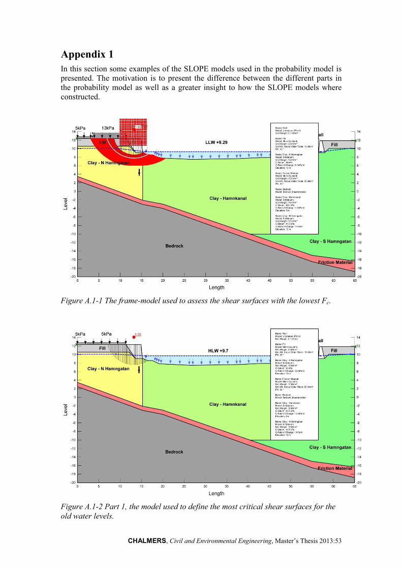
CHALMERS, Civil and Environmental Engineering, Master’s Thesis 2013:53 52
Appendix 1 In this section some examples of the SLOPE models used in the probability model is presented. The motivation is to present the difference between the different parts in the probability model as well as a greater insight to how the SLOPE models where constructed.
Figure A.1-1 The frame-model used to assess the shear surfaces with the lowest Fc.
Figure A.1-2 Part 1, the model used to define the most critical shear surfaces for the old water levels.

CHALMERS, Civil and Environmental Engineering, Master’s Thesis 2013:53 53
Figure A.1-3 Part 2 & 3, the model used to define the most critical shear surfaces for the new water levels.
Figure A.1-4 Part 3, the anisotropic model with the new water levels.

CHALMERS, Civil and Environmental Engineering, Master’s Thesis 2013:53 54
Figure A.1-5 Part 4, the model with the new water levels and pile forces (in this case 12 meter piles).
Figure A.1-6. Part 4, the anisotropic model with the new water levels and pile forces (in this case 8 meter piles).

CHALMERS, Civil and Environmental Engineering, Master’s Thesis 2013:53 55
Appendix 2
Figure A.2-1 Table of the percentiles from a standardized normal distribution (Alén, C et.al, 2012).

CHALMERS, Civil and Environmental Engineering, Master’s Thesis 2013:53 56
Appendix 3
13 kPa 1,03
0,178571 0,003571
LLW 8.9m 5 kPa 1,16
0,02 0,613095 0,012262
0 kPa 1,24
0,208333 0,004167
13 kPa 1,04
0,178571 0,057143
LW 9,1m 5 kPa 1,18
0,32 0,613095 0,19619
0 kPa 1,29
0,208333 0,066667
13 kPa 1,06
0,178571 0,057143
MLW 9,4m 5 kPa 1,18
0,32 0,613095 0,19619
0 kPa 1,33
0,208333 0,066667
13 kPa 1,09
0,178571 0,057143
HLW 9,7m 5 kPa 1,25
0,32 0,613095 0,19619
0 kPa 1,37
0,208333 0,066667
13 kPa 1,11
0,178571 0,003571

CHALMERS, Civil and Environmental Engineering, Master’s Thesis 2013:53 57
HHLW 9,9m 5 kPa 1,27
0,02 0,613095 0,012262
0 kPa 1,4
0,208333 0,004167 Figure A.3-1 Part 1 of the probability model.
13 kPa 1,05
0,178571 0,003571
LLW 9,29m 5 kPa 1,2
0,02 0,613095 0,012262
0 kPa 1,3
0,208333 0,004167
13 kPa 1,06
0,178571 0,057143
LW 9,41m 5 kPa 1,21
0,32 0,613095 0,19619
0 kPa 1,33
0,208333 0,066667
13 kPa 1,07
0,178571 0,057143
MLW 9,52m 5 kPa 1,22
0,32 0,613095 0,19619
0 kPa 1,34
0,208333 0,066667
13 kPa 1,08
0,178571 0,057143
HLW 9,62m 5 kPa 1,24

CHALMERS, Civil and Environmental Engineering, Master’s Thesis 2013:53 58
0,32 0,613095 0,19619
0 kPa 1,36
0,208333 0,066667
13 kPa 1,09
0,178571 0,003571
HHLW 9,74m 5 kPa 1,25
0,02 0,613095 0,012262
0 kPa 1,37
0,208333 0,004167 Figure A.3-2 Part 2 of the probability model.
13 kPa 1,15
0,178571 0,003571
LLW 9,29m 5 kPa 1,31
0,02 0,613095 0,012262
0 kPa 1,43
0,208333 0,004167
13 kPa 1,16
0,178571 0,057143
LW 9,41m 5 kPa 1,32
0,32 0,613095 0,19619
0 kPa 1,45
0,208333 0,066667
13 kPa 1,17
0,178571 0,057143
MLW 9,52m 5 kPa 1,34
0,32 0,613095 0,19619

CHALMERS, Civil and Environmental Engineering, Master’s Thesis 2013:53 59
0 kPa 1,47
0,208333 0,066667
13 kPa 1,18
0,178571 0,057143
HLW 9,62m 5 kPa 1,35
0,32 0,613095 0,19619
0 kPa 1,48
0,208333 0,066667
13 kPa 1,19
0,178571 0,003571
HHLW 9,74m 5 kPa 1,36
0,02 0,613095 0,012262
0 kPa 1,5
0,208333 0,004167 Figure A.3-3 Part 3 of the probability model.
5m 15,22 kN 1,25
0,107 0,000382
13 kPa 8m 22,17 kN 1,22
0,178571 0,75 0,002679
12m 14,7 kN 1,16
0,143 0,000511
5m 16,3 kN 1,47
0,107 0,001312
LLW 9,29m 5 kPa 8m 23,93 kN 1,43
0,02 0,613095 0,75 0,009196
12m 15,93 kN 1,35
0,143 0,001753

CHALMERS, Civil and Environmental Engineering, Master’s Thesis 2013:53 60
5m 26,89 kN 1,61
0,107 0,000446
0 kPa 8m 38,38 kN 1,61
0,208333 0,75 0,003125
12m 28,26 kN 1,52
0,143 0,000596
5m 15,22 kN 1,26
0,107 0,006114
13 kPa 8m 22,17 kN 1,23
0,178571 0,75 0,042857
12m 14,7 kN 1,18
0,143 0,008171
5m 16,3 kN 1,49
0,107 0,020992
LW 9,41m 5 kPa 8m 23,93 kN 1,45
0,32 0,613095 0,75 0,147143
12m 15,93 kN 1,36
0,143 0,028055
5m 16,3 kN 1,66
0,107 0,007133
0 kPa 8m 23,93 kN 1,61
0,208333 0,75 0,05
12m 15,93 kN 1,5
0,143 0,009533
5m 15,22 kN 1,27
0,107 0,006114

CHALMERS, Civil and Environmental Engineering, Master’s Thesis 2013:53 61
13 kPa 8m 22,17 kN 1,25
0,178571 0,75 0,042857
12m 14,7 kN 1,19
0,143 0,008171
5m 16,31 kN 1,51
0,107 0,020992
MLW 9,52m 5 kPa 8m 23,93 kN 1,47
0,32 0,613095 0,75 0,147143
12m 15,93 kN 1,38
0,143 0,028055
5m 16,31 kN 1,68
0,107 0,007133
0 kPa 8m 23,93 kN 1,63
0,208333 0,75 0,05
12m 15,93 kN 1,52
0,143 0,009533
5m 17,34 kN 1,31
0,107 0,006114
13 kPa 8m 25,59 kN 1,28
0,178571 0,75 0,042857
12m 17,11 kN 1,21
0,143 0,008171
5m 15,22 kN 1,52
0,107 0,020992
HLW 9,62m 5 kPa 8m 22,17 kN 1,49
0,32 0,613095 0,75 0,147143

CHALMERS, Civil and Environmental Engineering, Master’s Thesis 2013:53 62
12m 14,7 kN 1,39
0,143 0,028055
5m 16,31 kN 1,7
0,107 0,007133
0 kPa 8m 23,93 kN 1,65
0,208333 0,75 0,05
12m 15,93 kN 1,54
0,143 0,009533
5m 15,22 kN 1,3
0,107 0,000382
13 kPa 8m 22,17 kN 1,27
0,178571 0,75 0,002679
12m 14,7 kN 1,21
0,143 0,000511
5m 15,22 kN 1,54
0,107 0,001312
HHLW 9,74m 5 kPa 8m 22,17 kN 1,5
0,02 0,613095 0,75 0,009196
12m 14,7 kN 1,4
0,143 0,001753
5m 15,22 kN 1,74
0,107 0,000446
0 kPa 8m 22,17 kN 1,68
0,208333 0,75 0,003125
12m 14,7 kN 1,56
0,143 0,000596 Figure A.3-4 Part 4 of the probability model.

CHALMERS, Civil and Environmental Engineering, Master’s Thesis 2013:53 63
5m 15,22 kN 1,36
0,107 0,000382
13 kPa 8m 22,17 kN 1,33
0,178571 0,75 0,002679
12m 14,7 kN 1,27
0,143 0,000511
5m 16,3 kN 1,6
0,107 0,001312
LLW 9,29m 5 kPa 8m 23,93 kN 1,56
0,02 0,613095 0,75 0,009196
12m 15,93 kN 1,45
0,143 0,001753
5m 26,89 kN 1,75
0,107 0,000446
0 kPa 8m 38,38 kN 1,76
0,208333 0,75 0,003125
12m 28,26 kN 1,66
0,143 0,000596
5m 15,22 kN 1,38
0,107 0,006114
13 kPa 8m 22,17 kN 1,35
0,178571 0,75 0,042857
12m 14,7 kN 1,28
0,143 0,008171
5m 16,3 kN 1,62
0,107 0,020992
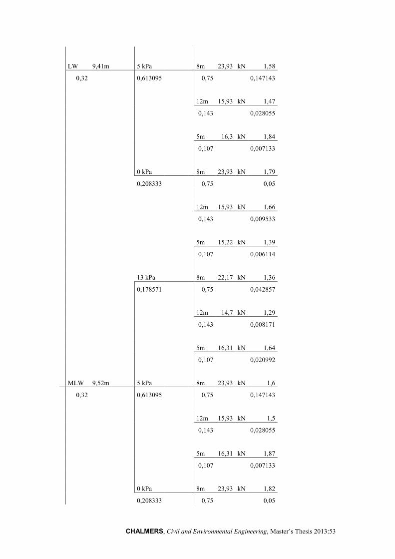
CHALMERS, Civil and Environmental Engineering, Master’s Thesis 2013:53 64
LW 9,41m 5 kPa 8m 23,93 kN 1,58
0,32 0,613095 0,75 0,147143
12m 15,93 kN 1,47
0,143 0,028055
5m 16,3 kN 1,84
0,107 0,007133
0 kPa 8m 23,93 kN 1,79
0,208333 0,75 0,05
12m 15,93 kN 1,66
0,143 0,009533
5m 15,22 kN 1,39
0,107 0,006114
13 kPa 8m 22,17 kN 1,36
0,178571 0,75 0,042857
12m 14,7 kN 1,29
0,143 0,008171
5m 16,31 kN 1,64
0,107 0,020992
MLW 9,52m 5 kPa 8m 23,93 kN 1,6
0,32 0,613095 0,75 0,147143
12m 15,93 kN 1,5
0,143 0,028055
5m 16,31 kN 1,87
0,107 0,007133
0 kPa 8m 23,93 kN 1,82
0,208333 0,75 0,05

CHALMERS, Civil and Environmental Engineering, Master’s Thesis 2013:53 65
12m 15,93 kN 1,68
0,143 0,009533
5m 17,34 kN 1,42
0,107 0,006114
13 kPa 8m 25,59 kN 1,39
0,178571 0,75 0,042857
12m 17,11 kN 1,32
0,143 0,008171
5m 15,22 kN 1,66
0,107 0,020992
HLW 9,62m 5 kPa 8m 22,17 kN 1,62
0,32 0,613095 0,75 0,147143
12m 14,7 kN 1,5
0,143 0,028055
5m 16,31 kN 1,89
0,107 0,007133
0 kPa 8m 23,93 kN 1,84
0,208333 0,75 0,05
12m 15,93 kN 1,7
0,143 0,009533
5m 15,22 kN 1,42
0,107 0,000382
13 kPa 8m 22,17 kN 1,39
0,178571 0,75 0,002679
12m 14,7 kN 1,32
0,143 0,000511

CHALMERS, Civil and Environmental Engineering, Master’s Thesis 2013:53 66
5m 15,22 kN 1,68
0,107 0,001312
HHLW 9,74m 5 kPa 8m 22,17 kN 1,64
0,02 0,613095 0,75 0,009196
12m 14,7 kN 1,53
0,143 0,001753
5m 15,22 kN 1,9
0,107 0,000446
0 kPa 8m 22,17 kN 1,84
0,208333 0,75 0,003125
12m 14,7 kN 1,71
0,143 0,000596 Figure A.3-5 Part 5 of the probability model.

CHALMERS, Civil and Environmental Engineering, Master’s Thesis 2013:53 67
Appendix 4
Figure A.4-1 Figure used to assess the value of τα/τhor (Axelsson et.al, 1995).
Numbers in the figure shows values for K0(NC)
α°
� �/� �
!