programing fundamentals - ucsb-bren. · pdf fileprograming fundamentals. modularity main...

❖ A program is a set of instructions for a computer to follow !

❖ Programs are often used to manipulate data (in all type and formats you discussed last week)!

❖ Simple to complex!

❖ the scripts you wrote last week (simple)!

❖ instructions to analyze relationships in census data and visualize them!

❖ a model of global climate

Programing fundamentals

❖ Programs can be written in many different languages (all have their strengths and weakness)!

❖ Languages expect instructions in a particular form (syntax) and then translate them to be readable by the computer!

❖ Languages have evolved to make it help users write programs that are easy to understand, re-use, extend, test, run quickly, use lots of data…


❖ Operations (=,+,-,…concatenate, copy)!

❖ Data structures (simple variables, arrays, lists…)!

❖ Control structures (if then, loops)!

❖ Modules…!

!

Concepts common to all languages through the syntax may be different


Modularity

Main controls the overall flow of program- calls to the functions/

modules/building blocks

Functions - the modules/boxes

Functions - the modules/boxes

Functions - the modules/boxes Functions - the

modules/boxes Functions - the modules/boxes

❖ A program is often multiple pieces put together!

❖ These pieces or modules can be used multiple times

❖ Modularity!

❖ breaking your instructions down into individual pieces!

❖ identifying instructions that can be reused!

❖ an ecosystem model might re-use instructions for calculating how a species grows!

❖ an accounting program might re-use instructions for computing net present value from interest rates!

❖ modules often become ‘black boxes’ which hides detail that might make understanding the program overly complex!

❖ most languages have lots of black boxes already written and most allow you to write your own


❖ Read: Wilson G, Aruliah DA, Brown CT, Chue Hong NP, Davis M, et al. (2014) Best Practices for Scientific Computing. PLoS Biol 12(1): e1001745. doi:10.1371/journal.pbio.1001745!

❖ Blanton, B and Lenhardt, C 2014. A Scientist’s Perspective on Sustainable Scientific Software. Journal of Open Research Software 2(1):e17, DOI: http://dx.doi.org/10.5334/jors.ba!

❖ but also!

❖ http://simpleprogrammer.com/2013/02/17/principles-are-timeless-best-practices-are-fads/

Best practices for software development

http://simpleprogrammer.com/2013/02/17/principles-are-timeless-best-practices-are-fads/

Best practices for model (software) development

❖ Common problems!

❖ Unreadable code (hard to understand, easy to forget how it works, hard to find errors, hard to expand)!

❖ Overly complex, disorganized code (hard to find errors; hard to modify-expand)!

❖ Insufficient testing (both during development and after)!

❖ Not tracking code changes (multiple versions, which is correct?)

Steps for building model!

❖ We are going to use R; but the basic design of programs are similar across many programming languages!

❖ Why R?!

❖ Free (and open source) software!

❖ Good (and getting better) visualization tools !

❖ Growing user community who make their R code available!

❖ ( currently 2800+ user packages on CRAN R server)!

❖ Links with other tools and languages (GIS, Python, C, C++…)!

❖ Built in tools to deal with space and time!

❖ Lots of user support

Steps for building model

!

❖ Why not R?!

❖ Not particularly computationally efficient (e.g slow for repetitive computations) ; hard to parallelize!

❖ Not the right tool for developing really complex models (you don’t develop GCMs in R!)

STEPS: Program Design

1. Clearly define your goal as precisely as possible, what do you want your program to do!

1. inputs/parameters!

2. outputs!

2. Implement and document!

3. Test !

4. Refine

Steps for building a module

!1. Design the program “conceptually” - “on paper” in words or figures!2. Translate into a step by step representation!3. Choose programming language!4. Define inputs (data type, units)!5. Define output (data type, units)!6. Define structure!7. Write program!8. Document the program !9. Test the program!10. Refine…

ModuleInput Output

Parameters

Best practices for model (software) development❖ Let us change our traditional attitude to the construction of

programs: Instead of imagining that our main task is to instruct a computer what to do, let us concentrate rather on explaining to humans what we want the computer to do. -- Donald E. Knuth, Literate Programming, 1984!

❖ Developing readable (by PEOPLE) code and documenting what you are doing is essential!

❖ “When was the last time you spent a pleasant evening in a comfortable chair, reading a good program?”— Bentley (1986)


❖ Automated tools (useful for more complex code development !

❖ ( note that GP’s often create programs > 100 lines of code)!

❖ Automated documentation!

❖ http://www.stack.nl/~dimitri/doxygen/!

❖ http://roxygen.org/roxygen2-manual.pdf !

❖ Automated test case development!

❖ http://r-pkgs.had.co.nz/tests.html!

❖ Automated code evolution tracking (Version Control)!

❖ https://github.com/

http://www.stack.nl/~dimitri/doxygen/

http://roxygen.org/roxygen2-manual.pdf

http://r-pkgs.had.co.nz/tests.html

https://github.com/

Designing Programs❖ Inputs - sometimes separated into input data and parameters!

❖ input data = the “what” that is manipulated!

❖ parameters determine “how” the manipulation is done!

❖ “sort -n file.txt”!

❖ sort is the program - set of instructions - its a black box!

❖ input is file.txt!

❖ parameters is -n!

❖ output is a sorted version of file.txt!

❖ my iphone app for calculating car mileage!

❖ inputs are gallons and odometer readings at each fill up !

❖ graph of is miles/gallon over time !

❖ parameters control units (could be km/liter, output couple be presented as a graph or an average value)

Designing Programs

❖ What’s in the box (the program itself) that gives you a relationship between outputs and inputs!

❖ the link between inputs and output !

❖ breaks this down into bite-sized steps or calls to other boxes) !

❖ think of programs as made up building blocks!

❖ the design of this set of sets should be easy to follow!

Building Blocks

❖ Instructions inside the building blocks/box!

❖ Numeric data operators!

❖ +,-,/,*, %*%!

❖ Strings!

❖ substr, paste..!

❖ Math!

❖ sin, cos, exp, min, max…!

❖ these are themselves programs - boxes!

❖ R-reference card is useful!


❖ Structured practices that ensures!

❖ clear, readable code!

❖ modularity (organized “independent” building blocks)!

❖ testing as you go and after !

❖ code evolution is documented

Building Blocks

❖ Functions (or objects or subroutines)!!

❖ The basic building blocks !

❖ Functions can be written in all languages; in many languages (object-oriented) like C++, Python, functions are also objects!

❖ Functions are the “box” of the model - the transfer function that takes inputs and returns outputs!

❖ More complex models - made up of multiple functions; and nested functions (functions that call/user other functions)

Functions in R❖ Format for a basic function in R!

!#’ documentation that describes inputs, outputs and what the function does!

FUNCTION NAME = function(inputs, parameters) {!

body of the function (manipulation of inputs)!

return(values to return)!

}!

!In R, inputs and parameters are treated the same; but it is useful to think about them separately in designing the model - collectively they are sometimes referred to as arguments!

!ALWAYS USE Meaningful names for your function, its parameters and variables calculated within the function

A simple program: Example

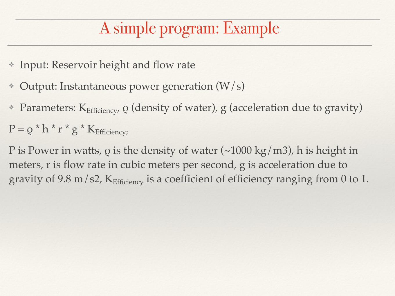
❖ Input: Reservoir height and flow rate !

❖ Output: Instantaneous power generation (W/s)!

❖ Parameters: KEfficiency, ρ (density of water), g (acceleration due to gravity)!

P = ρ * h * r * g * KEfficiency; !

P is Power in watts, ρ is the density of water (~1000 kg/m3), h is height in meters, r is flow rate in cubic meters per second, g is acceleration due to gravity of 9.8 m/s2, KEfficiency is a coefficient of efficiency ranging from 0 to 1. !

!

Building Models

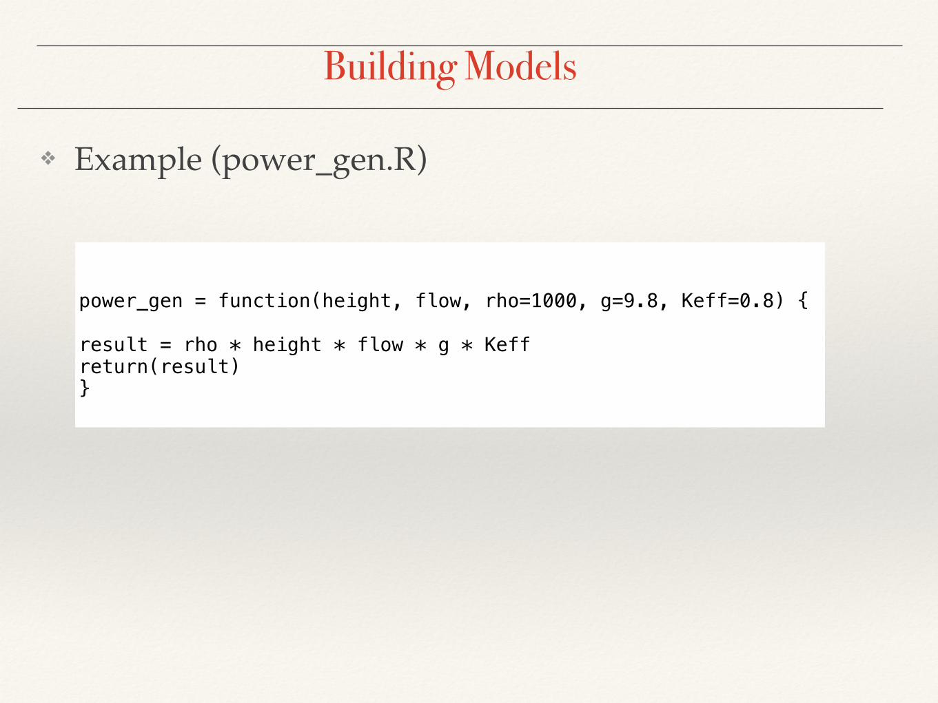
❖ Example (power_gen.R)

!!power_gen = function(height, flow, rho=1000, g=9.8, Keff=0.8) { !result = rho * height * flow * g * Keff return(result) } !

Building Models

❖ Inputs/parameters are height, flow, rho, g, and K!

❖ For some (particularly parameters) we provide default values by assigning them a value (e.g Keff = 0.8), but we can overwrite these!

❖ Body is the equations between { and }!

❖ return tells R what the output is

!!power_gen = function(height, flow, rho=1000, g=9.8, Keff=0.8) { !result = rho * height * flow * g * Keff return(result) } !

Arguments to the function follow the order they are listed in your definition!Or you can specify which argument you are referring to when you call the program!!!power_gen = function(height, flow, rho=1000, g=9.8, K=0.8) { !# calculate power result = rho * height * flow * g * K return(result) } !

Building Models: Using the model

Building Models

❖ Always write your function in a text editor and then copy into R!

❖ By convention we name files with functions in them by the name of the function.R!

❖ so power_gen.R!

❖ you can also have R read a text file by source(“power_gen.R”) - make sure you are in the right working directory!

❖ Eventually we will want our function to be part of a package (a library of many functions) - to create a package you must use this convention (name.R)

Defaults take the value they were assigned in the definition,! but can be overwritten!

!power_gen = function(height, flow, rho=1000, g=9.8, K=0.8) { !# calculate power result = rho * height * flow * g * K return(result) } !

Building Models: Using the model

> power_gen!function(height, flow, rho=1000, g=9.8, K=0.8) {! ! # calculate power! result = rho * height * flow * g * K! return(result)!}!> result!Error: object 'result' not found!> K!Error: object 'K' not found!>

ScopingThe scope of a variable in a program defines where it can be “seen”!!Variables defined inside a function cannot be “seen” outside of that function!!There are advantages to this - the interior of the building block does not ‘interfere’ with other parts of the program!!

Building Models: Using the modelOne of the equations used to compute automobile fuel efficiency is as follows this is the power required to keep a car moving at a given speed!!Pb = crolling * m *g*V + 1/2 A*pair*cdrag*V3!!where crolling and cdrag are rolling and aerodynamic resistive!coefficients, typical values are 0.015 and 0.3, respectively.!V: is vehicle speed (assuming no headwind) in m/s (or mps)!m: is vehicle mass in kg !A is surface area of car (m2)!g: is acceleration due to gravity (9.8 m/s2)!pair = density of air (1.2kg/m3)!Pb is power in Watts!!Write a function to compute power, given a truck of m=31752 kg (parameters for a heavy truck) for a range of different highway speeds!plot power as a function of speed!how does the curve change for a lighter vehicle!!Note that 1mph=0.477m/s!

!!

Simple Functions

!!power = function(cdrag=0.3, crolling=0.015,pair=1.2,g=9.8,V,m,A) { P = crolling*m*g*V + 1/2*A*pair*cdrag*V**3 return(P) } !v=seq(from=0, to=100, by=10) plot(v, power(V=0.447*v, m=31752, A=25)) lines(v, power(V=0.447*v, m=61752, A=25)) !

Simple Functions!#' Power Required by Speed #' #' This function determines the power required to keep a vehicle moving at #' a given speed #' @param cdrag coefficient due to drag default=0.3 #' @param crolling coefficient due to rolling/friction default=0.015 #' @param v vehicle speed (m/2) #' @param m vehicle mass (kg) #' @param A area of front of vehicle (m2) #' @param g acceleration due to gravity (m/s) default=9.8 #' @param pair (kg/m3) default =1.2 #' @return power (W) !power = function(cdrag=0.3, crolling=0.015,pair=1.2,g=9.8,V,m,A) { P = crolling*m*g*V + 1/2*A*pair*cdrag*V**3 return(P) } !v=seq(from=0, to=100, by=10) plot(v, power(V=0.447*v, m=31752, A=25)) lines(v, power(V=0.447*v, m=61752, A=25)) !

Key Programming concepts: Review of data types!

❖ Understanding data types is important for designing your model I/O; specifying what the model will do!

❖ Data types and data structures are necessary for creating more complex inputs and outputs!

❖ All programming languages have sets of data types !

❖ single values: character, integer, real, logical/boolean (Y/N)!

❖ data structures: arrays, vectors, matrices, !

❖ in R core types; dataframes, lists, factors!

❖ in R defined types: spatial, date…

Building Programs

A core issue in modeling (both designing and using) are the data structures/formats used to hold data that is input and output from programs: In good programs, data structures support organization and program flow and readability

MODEL

Complex data: time, space, conditions!and their interactions

Key Programming concepts: Data types and structures

❖ Good data structures are:!

❖ as simple as possible!

❖ easy understand (readable names, and sub-names)!

❖ easy to manipulate (matrix operations, applying operations by category)!

❖ easy to visualize (graphs and other display)

Key Programming concepts: Review of data types

❖ Vectors - a 1-dimensional set of numbers!

❖ a = c(1,5,8, 4, 22,33) !

❖ Matrix - a 2-dimensional set of numbers (organized in rows and columns)!

❖ b = matrix(a, nrow=2, ncol=3)


❖ You can also define an “empty” matrix to fill values in later !

❖ think of creating a data structure to store energy production in winter and summer for 6 different power plants)!

❖ res = matrix(nrow=2, ncol=6)


❖ You can combine vectors into a matrix using!

❖ cbind by columns!

❖ rbind by rows


❖ A really useful data structure in R is a data frame!

❖ Dataframe’s are like matrices = they have rows and columns but they don’t have to be numeric (although they can be)!

❖ Useful if you have data that is of mixed type

Data Frame Creation Example


Adding columns

seq - a sequence of number from to by!rnorm - generate, n numbers from a normal distribution with a given mean and standard deviation


❖ Of course we can use matrices/data frames as inputs/output for our models!

❖ Example using our power_gen model from earlier - using vectors instead of single values

Key Programming concepts: Review of data types❖ Why does this work?!

❖ Because height, flow columns are both from reservoir.operation (a data frame) so they are vectors of the SAME length!

❖ So when you multiply height* flow, you multiply!

❖ height[1]*flow[1],,, and then height[2]*flow[2] etc


❖ Matrix multiplication is different!

❖ in R, this would be !

❖ k %*% m!

!

❖ Matrix multiplication is often used within certain types of models…we will get to examples later


Adding columns


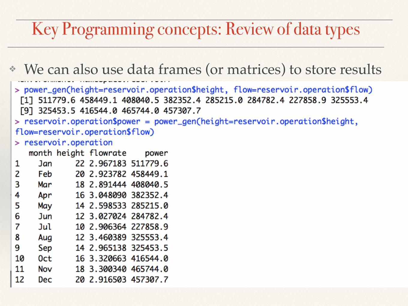
❖ We can also use data frames (or matrices) to store results


❖ Some other useful commands!

❖ with - allows you to use the names of columns in the data frame directly!

❖ summary - summaries of columns (max, min, mean…)

Jan Feb Mar Apr May Jun Jul Aug Sep Oct Nov Dec

Pow

er (W

/s)

0e+00

2e+05

4e+05

Summary

Key Programming concepts: Review of data types❖ We can also use other functions and built in R functions

(like mean, lm, sum) within our function !

❖ Lets say we want to commute total annual power generated, given our inputs of average height and flow for each month? !

❖ what additional information would we need?

!#' Total Power Generation #' #' This function computes total power generation from a reservoir given its height and flow rate into turbines and number of days (and secs) within those days that the turbines are in operation #' @param rho Density of water (kg/m3) Default is 1000 #' @param g Acceleration due to gravity (m/sec2) Default is 9.8 #' @param Keff Turbine Efficiency (0-1) Default is 0.8 #' @param height height of water in reservoir (m) #' @param flow flow rate (m3/sec) #' @param number of days #' @param secs in days Default is 86400 #' @author Naomi #' @examples power_gen(20, 1, 10) #' @return Power generation (MW) !power_gen_total = function(height, flow, days, secs=86400, rho=1000, g=9.8, Keff=0.8) { !result = rho * height * flow * g * Keff result = result * days * secs total = sum(result)/1e6 !return(total) } !> > power_gen_total(reservoir.operation$height, reservoir.operation$flowrate, days=30) [1] 11702915 >

In Class example

❖ Expand your function that computes the power need to compute and return the total power given an input vector of different speeds and the time period over which those speeds are driven (we will ignore acceleration effect)!

!


❖ Arrays are like matrices but can be multi-dimensional!

❖ dim defines the dimensions of an array and gives the number of values in each dimension!

❖ a matrix is a 2-dimensional array!

❖ test = array(dim=c(2,5)) - this has 2 rows and 5 columns!

❖ You can have N-dimensional arrays

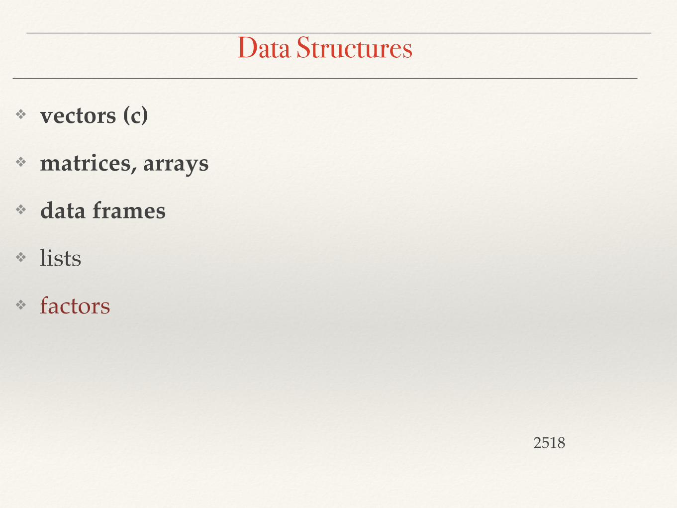
Data Structures

❖ vectors (c)!

❖ matrices, arrays!

❖ data frames!

❖ lists!

❖ factors

2518

Key Programming concepts: Review of data types❖ Factors (a bit tricky, basically a vector of “things” that has

different levels (classes); not really numeric - so you can’t average them!)!

❖ But can be useful for doing “calculations” with categories


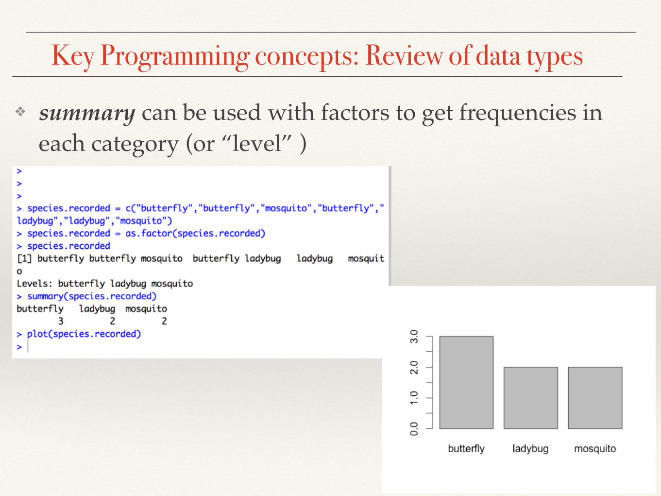
❖ summary can be used with factors to get frequencies in each category (or “level” )

You can “do things” (apply functions) to the summary (frequency of each “factor”

level


❖ A simple model that takes advantage of factors!

❖ A model to compute an index of species diversity from a list of recorded species

where n is the number of individuals in each species, and N is total number


#' Simpson's Species Diversity Index!#'!#' Compute a species diversity index!#' @param species list of species (names, or code)!#' @return value of Species Diversity Index!#' @examples!#' compute_simpson_index(c(“butterfly","butterfly","mosquito","butterfly",!#’ ”ladybug","ladybug")))!#' @references!#' http://www.tiem.utk.edu/~gross/bioed/bealsmodules/simpsonDI.html!!compute_simpson_index = function(species) {!!species = as.factor(species)!tmp = (summary(species)/sum(summary(species))) ** 2!diversity = sum(tmp)!return(diversity)!}!!

Data Structures

❖ a bit more on factors; a list of numbers can also be a factor but then they are not treated as actual numbers - you could think of them as “codes” or addresses or..!

❖ use as.numeric or as.character to go back to a regular vector from a factor

Data Structures

❖ vector, (c)!

❖ matrices, arrays!

❖ data frames!

❖ lists!

❖ factors


❖ Lists are the most “informal” data structures in R!

❖ List are really useful for keeping track of and organizing groups of things that are not all the same!

❖ A list could be a table where number of rows is different for each column!

❖ A list can have numeric, character, factors all mixed together!

❖ List are often used for returning more complex information from function (e.g. lm)


❖ A simple list!!> sale = list(2,"highquality","apple",4)!> sale![[1]]![1] 2!![[2]]![1] "highquality"!![[3]]![1] "apple"!![[4]]![1] 4!!


❖ A simple list: using names to identify elements!

> sale = list(number=2, quality="high", what="apple", cost=4)!> sale!$number![1] 2!!$quality![1] "high"!!$what![1] "apple"!!$cost![1] 4!!

Lists> !> costs = c(20,40,22, 32, 5)!> quality = c("G","G","F","G","B")!> purchased = c(33,5,22,6,7)!> !> sales = data.frame(costs=costs, quality=quality, purchased=purchased)!> !> !> sales! costs quality purchased!1 20 G 33!2 40 G 5!3 22 F 22!4 32 G 6!5 5 B 7!>

!>costs = c(73,44) >quality = c("G","G") >purchased = c(100,22) !>sales2 = data.frame(costs=costs, quality=quality, purchased=purchased) !

With lists we can combine sales data frames from two different places into a single data structure

Lists

❖ mar> > markets = list(site1=sales, site2=sales2) > markets $site1 costs quality purchased 1 20 G 33 2 40 G 5 3 22 F 22 4 32 G 6 5 5 B 7 !$site2 costs quality purchased 1 73 G 100 2 44 G 22 !> markets[[1]]$costs [1] 20 40 22 32 5 > > markets$site1$costs [1] 20 40 22 32 5 >

Lists> > > markets[[1]] costs quality purchased 1 20 G 33 2 40 G 5 3 22 F 22 4 32 G 6 5 5 B 7 > > markets[[2]] costs quality purchased 1 73 G 100 2 44 G 22 > > > markets[[1]][1,3] [1] 33 >

[[]] is used to get elements from the list


❖ one of the most useful things to do with list is to use them to return multiple ‘items’ from a function!

#' computes profit from price for forest plot and Mg/C in that plot #' @param price ($) #' @param carbon (MgC) #' @return list with mean, min, and max prices compute_carbonvalue = function(price, carbon) { !cost.per.carbon = price/carbon a = mean(cost.per.carbon) b = max(cost.per.carbon) c = min(cost.per.carbon) !result = list(avg=a, min=c, max=b) return(result) }


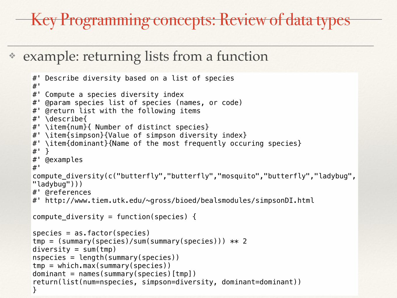
❖ example: returning lists from a function!

> > obs = data.frame(prices=c(23,44,60,4,2,33,59), forestC=c(59,88,100,10,8,79,300)) > obs prices forestC 1 23 59 2 44 88 3 60 100 4 4 10 5 2 8 6 33 79 7 59 300 > forest.res = compute_carbonvalue(obs$prices, obs$forestC) > forest.res $avg [1] 0.3934598 !$min [1] 0.1966667 !$max [1] 0.6 !>


❖ example: returning lists from a function!> obs=data.frame(prices=c(18,2,12,5), grassC=c(22,3,19,8)) > grass.res=compute_carbonvalue(obs$prices, obs$grassC) > grass.res $avg [1] 0.6853569 !$min [1] 0.625 !$max [1] 0.8181818 !>

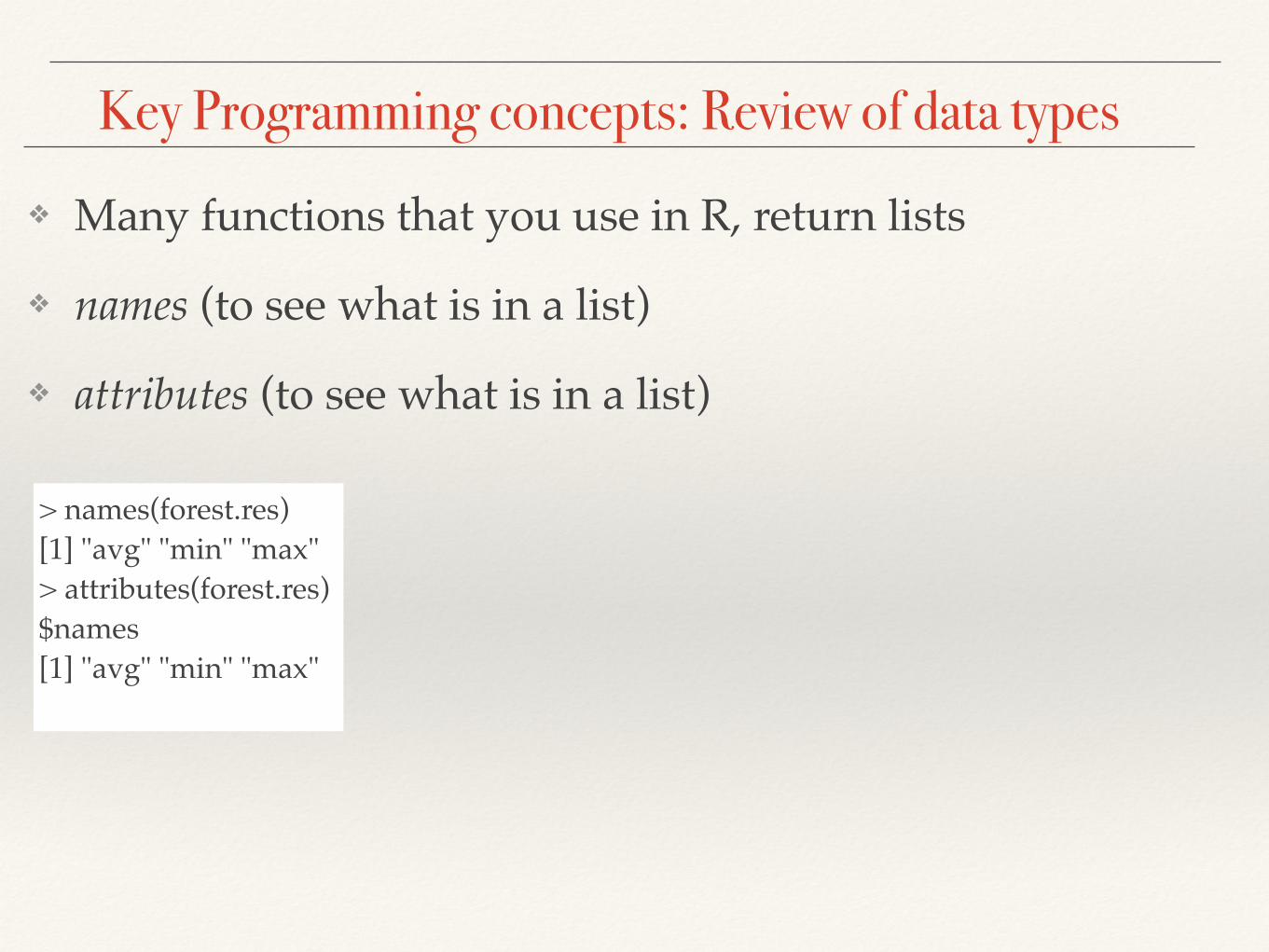
❖ Many functions that you use in R, return lists!

❖ names (to see what is in a list)!

❖ attributes (to see what is in a list)


> names(forest.res)![1] "avg" "min" "max"!> attributes(forest.res)!$names![1] "avg" "min" "max"!

❖ lm is an example of a function that returns a list

Key Programming concepts: Review of data types> !> res = lm(obs$prices~obs$forestC)!> names(res)! [1] "coefficients" "residuals" "effects" ! [4] "rank" "fitted.values" "assign" ! [7] "qr" "df.residual" "xlevels" ![10] "call" "terms" "model" !> res$coefficients!(Intercept) obs$forestC ! 14.9789368 0.1865644 !> res$model! obs$prices obs$forestC!1 23 59!2 44 88!3 60 100!4 4 10!5 2 8!6 33 79!7 59 300!>


❖ example: returning lists from a function!#' Describe diversity based on a list of species #' #' Compute a species diversity index #' @param species list of species (names, or code) #' @return list with the following items #' \describe{ #' \item{num}{ Number of distinct species} #' \item{simpson}{Value of simpson diversity index} #' \item{dominant}{Name of the most frequently occuring species} #' } #' @examples #' compute_diversity(c("butterfly","butterfly","mosquito","butterfly","ladybug","ladybug"))) #' @references #' http://www.tiem.utk.edu/~gross/bioed/bealsmodules/simpsonDI.html !compute_diversity = function(species) { !species = as.factor(species) tmp = (summary(species)/sum(summary(species))) ** 2 diversity = sum(tmp) nspecies = length(summary(species)) tmp = which.max(summary(species)) dominant = names(summary(species)[tmp]) return(list(num=nspecies, simpson=diversity, dominant=dominant)) }

❖ to your function that computes power, also return!

❖ an array that contains both power for each input speed!

❖ total power


Key Programming concepts: Review of data typessd

http://www.simonqueenborough.com/R/basic/figure/data-types.png

Key Programming concepts: Looping

❖ Loops are fundamental in all programming languages: and are frequently used in models


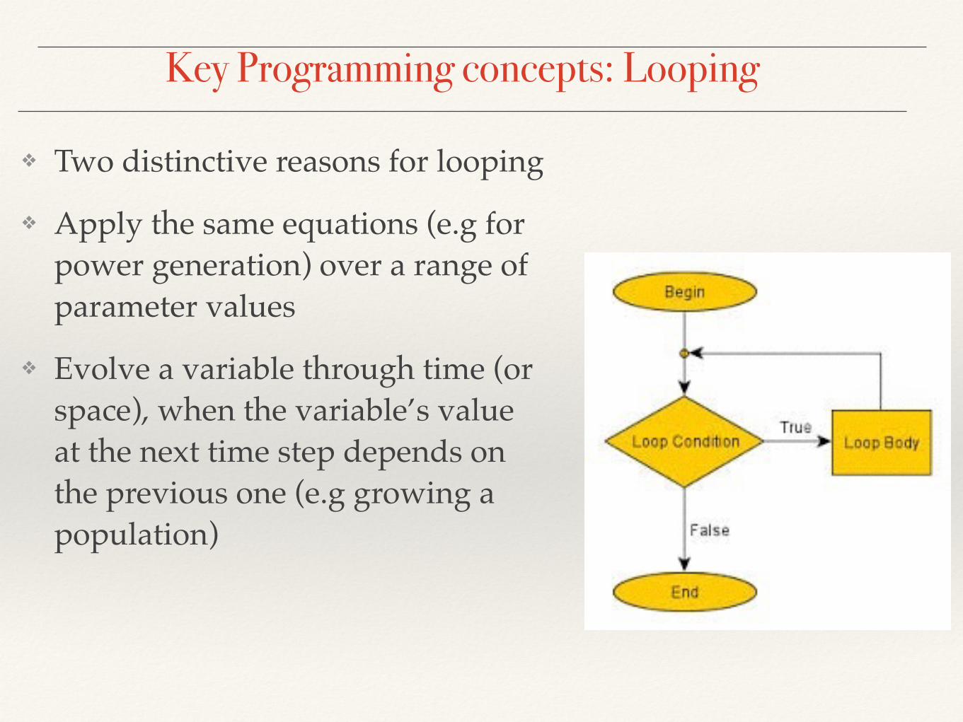
❖ Two distinctive reasons for looping!

❖ Apply the same equations (e.g for power generation) over a range of parameter values!

❖ Evolve a variable through time (or space), when the variable’s value at the next time step depends on the previous one (e.g growing a population)


❖ All loops have this basic structure - repeat statements (loop body) until a condition is true


❖ In R, the most commonly used loop is the For loop!

❖ for (i in 1:n) { statements}!

❖ In “for” loops the i (or whatever variable you want to use as the counter, is automatically incremented each time the loop is gone through; and the looping ends when i (the counter) reaches n!

❖ What is x? alpha? after this loop is run>x=0!> for (alpha in 1:4) { x = x+alpha}!

> !> !> x=0!> for (alpha in 1:4) { x = x+alpha}!> !> !> alpha![1] 4!> x![1] 10!


❖ Loops can be “nested” - one loop inside the other!

❖ For example, if we want to calculate NPV for a range of different interest rates and a range of damages that may be incurred 10 years in the future !

❖ using a function called compute_npv!

❖ Steps!

❖ define inputs (interest rates, damages)!

❖ define a data structure to store results!

❖ define function/model (already available)!

❖ use looping to run model for all inputs and store in data structure

Key Programming concepts: Looping> !> !> damages = c(25,33,91,24)!> discount.rates = seq(from=0.01, to=0.04, by=0.005)!> yr=10!> npvs = as.data.frame(matrix(nrow=length(damages), ncol=length(discount.rates)))!> for (i in 1:length(damages)) {!+ for (j in 1:length(discount.rates)) {!+ npvs[i,j]= compute_npv(net=damages[i], dis=discount.rates[j],yr )!+ }!+ }!> npvs! V1 V2 V3 V4 V5 V6 V7!1 22.63217 21.54168 20.50871 19.52996 18.60235 17.72297 16.88910!2 29.87447 28.43502 27.07149 25.77955 24.55510 23.39432 22.29362!3 82.38111 78.41172 74.65170 71.08905 67.71255 64.51161 61.47634!4 21.72689 20.68001 19.68836 18.74876 17.85825 17.01405 16.21354!> colnames(npvs)=discount.rates!> rownames(npvs)=damages!> npvs! 0.01 0.015 0.02 0.025 0.03 0.035 0.04!25 22.63217 21.54168 20.50871 19.52996 18.60235 17.72297 16.88910!33 29.87447 28.43502 27.07149 25.77955 24.55510 23.39432 22.29362!91 82.38111 78.41172 74.65170 71.08905 67.71255 64.51161 61.47634!24 21.72689 20.68001 19.68836 18.74876 17.85825 17.01405 16.21354!>


❖ Another useful looping construct is the While loop!

❖ keep looping until a condition is met!

❖ Useful when you don’t know what “n” in the for 1 in to “n” is!

❖ often used in models where you are evolving!

❖ accumulate something until a threshold is reached (population, energy, biomass?


❖ A simple while loop example !

!

!

!

!

!

❖ alpha = (1+2+3+4+5+6+7+8+9+10+11+12+13+14) = 105

> !> !> alpha = 0!> x = 0 !> while (alpha < 100) { alpha = alpha + x; x = x+1}!> x![1] 15!> alpha![1] 105!>


❖ A more useful while loop example!

❖ A question: if a metal toxin in a lake increases by 1% per year, how many years will it take for the metal level to be greater than 30 units, if toxin is current at 5 units!

❖ there are other ways to do this, but a while loop would do it > > !

> pollutant.level = 5!> while (pollutant.level < 30 ) {!+ pollutant.level = pollutant.level + 0.01* pollutant.level!+ yr = yr + 1!+ }!>

why won’t this work?


> yr=1!> pollutant.level = 5!> while (pollutant.level < 30 ) {!+ pollutant.level = pollutant.level + 0.01* pollutant.level!+ yr = yr + 1!+ }!> > yr![1] 182!> pollutant.level![1] 30.2788!


❖ Most programming languages have For and while loops

Python Programming, 1/e 36

File Loops # average5.py # Computes the average of numbers listed in a file. def main(): fileName = raw_input("What file are the numbers in? ") infile = open(fileName,'r') sum = 0.0 count = 0 for line in infile.readlines(): sum = sum + eval(line) count = count + 1 print "\nThe average of the numbers is", sum / count

mcsp.wartburg.edu/zelle/python/ppics1/.../Chapter08.p

Key Programming concepts: Control Structures❖ if(cond) expression

> !> a=4!> b=10!> if(a > b) win = "a"!> if(b > a) win = "b"!> win![1] "b"!>

❖ ifelse(cond, true, false)>!> win = ifelse(a > b, "a","b")!> win![1] "b"!> !>

Conditions:!== equal!> greater than!>= greater than or equal to!< less than!<= less than or equal to!%in% is in a list of something

&& AND!|| OR!

is.null()

Key Programming concepts: Looping❖ Inside functions if(cond) {expression} else {expression}!

❖ the expression can always have multiple statements using {}!

❖ If can be useful for branching in your model

Key Programming concepts: Control Structures

#' compute annual yield #' #' Function to compute yeild of different fruits as a function of annual temperature and precipitation #' @param T annual temperature (C) #' @param P annual precipitation (mm) #' @param ts slope on temperature #' @param tp slope on precipitation #' @param intercept (kg) #' @param irr Y or N (default N) #' @return yield in kg !!compute_yield = function(T, P, ts, tp, intercept, irr="N") { !if (irr=="N"){ yield = tp*P + ts*T + intercept } else { yield = ts*T + intercept } !return(yield) } !

!> !> compute_yield(32,200, 0.2, 0.4, 500)![1] 586.4!> compute_yield(32,200, 0.2, 0.4, 500, "N")![1] 586.4!> compute_yield(32,200, 0.2, 0.4, 500, "Y")![1] 506.4!

If can also be useful for creating classes of variables!!Lets say we want to build a function that will compute mean spring, winter, summer, streamflow - from a dataset that looks something like this!!!

!!> summary(streamflow)! year month day mm ! Min. :1953 Min. : 1.000 Min. : 1.00 Min. : 0.08996 ! 1st Qu.:1967 1st Qu.: 4.000 1st Qu.: 8.00 1st Qu.: 0.24290 ! Median :1981 Median : 7.000 Median :16.00 Median : 0.38685 ! Mean :1981 Mean : 6.542 Mean :15.73 Mean : 1.07800 ! 3rd Qu.:1995 3rd Qu.:10.000 3rd Qu.:23.00 3rd Qu.: 0.98961 ! Max. :2010 Max. :12.000 Max. :31.00 Max. :71.97168 !> !> head(streamflow)! year month day mm!1 1953 10 1 0.2608973!2 1953 10 2 0.2608973!

> !> !> streamflow$season = ifelse(streamflow$month %in% c(1,2,3,10,11,12),"winter","summer")!> head(streamflow)! year month day mm season!1 1953 10 1 0.2608973 winter!2 1953 10 2 0.2608973 winter!3 1953 10 3 0.2608973 winter!4 1953 10 4 0.2608973 winter!5 1953 10 5 0.2608973 winter!6 1953 10 6 0.2608973 winter!> plot(streamflow$season)!Error in plot.window(...) : need finite 'ylim' values!In addition: Warning messages:!1: In xy.coords(x, y, xlabel, ylabel, log) : NAs introduced by coercion!2: In min(x) : no non-missing arguments to min; returning Inf!3: In max(x) : no non-missing arguments to max; returning -Inf!> plot(as.factor(streamflow$season))!>

summer winter

02000

4000

6000

8000

10000

> !!> plot(as.factor(streamflow$season))!>

#’ @param str data frame with columns month and mm (mm is daily streamflow) compute_seasonal_meanflow = function(str) { !str$season = ifelse( str$month %in% c(1,2,3,10,11,12),"winter","summer") !tmp = subset(str, str$season=="winter") mean.winter = mean(tmp$mm) !tmp = subset(str, str$season=="summer") mean.summer = mean(tmp$mm) return(list(summer=mean.summer, winter=mean.winter)) } !!

> compute_seasonal_meanflow(streamflow)!$summer![1] 1.538304!!$winter![1] 0.6200728!!>


If can also be used to choose what you return from a function!compute_seasonal_flow = function(str,kind) { !str$season = ifelse( str$month %in% c(1,2,3,10,11,12),"winter","summer") !tmp = subset(str, str$season=="winter") if(kind=="mean") winter= mean(tmp$mm) if(kind=="max") winter= max(tmp$mm) if(kind=="min") winter=min(tmp$mm) !tmp = subset(str, str$season=="summer") if(kind=="mean") summer= mean(tmp$mm) if(kind=="max") summer= max(tmp$mm) if(kind=="min") summer=min(tmp$mm) !!return(list(summer=summer, winter=winter)) }

summer winter

02000

4000

6000

8000

10000

> !!> plot(as.factor(streamflow$season))!>

#’ @param str data frame with columns month and mm (mm is daily streamflow) compute_seasonal_meanflow = function(str) { !str$season = ifelse( str$month %in% c(1,2,3,10,11,12),"winter","summer") !tmp = subset(str, str$season=="winter") mean.winter = mean(tmp$mm) !tmp = subset(str, str$season=="summer") mean.summer = mean(tmp$mm) return(list(summer=mean.summer, winter=mean.winter)) } !!

> compute_seasonal_meanflow(streamflow)!$summer![1] 1.538304!!$winter![1] 0.6200728!!>


If can also be used to choose what you return from a function!compute_seasonal_flow = function(str,kind) { !str$season = ifelse( str$month %in% c(1,2,3,10,11,12),"winter","summer") !tmp = subset(str, str$season=="winter") if(kind=="mean") winter= mean(tmp$mm) if(kind=="max") winter= max(tmp$mm) if(kind=="min") winter=min(tmp$mm) !tmp = subset(str, str$season=="summer") if(kind=="mean") summer= mean(tmp$mm) if(kind=="max") summer= max(tmp$mm) if(kind=="min") summer=min(tmp$mm) !!return(list(summer=summer, winter=winter)) }


If can also be used to choose what you return from a function

> !> !> compute_seasonal_flow(streamflow,"mean")!$summer![1] 1.538304!!$winter![1] 0.6200728!!> compute_seasonal_flow(streamflow,"max")!$summer![1] 23.66069!!$winter![1] 71.97168!!

Example

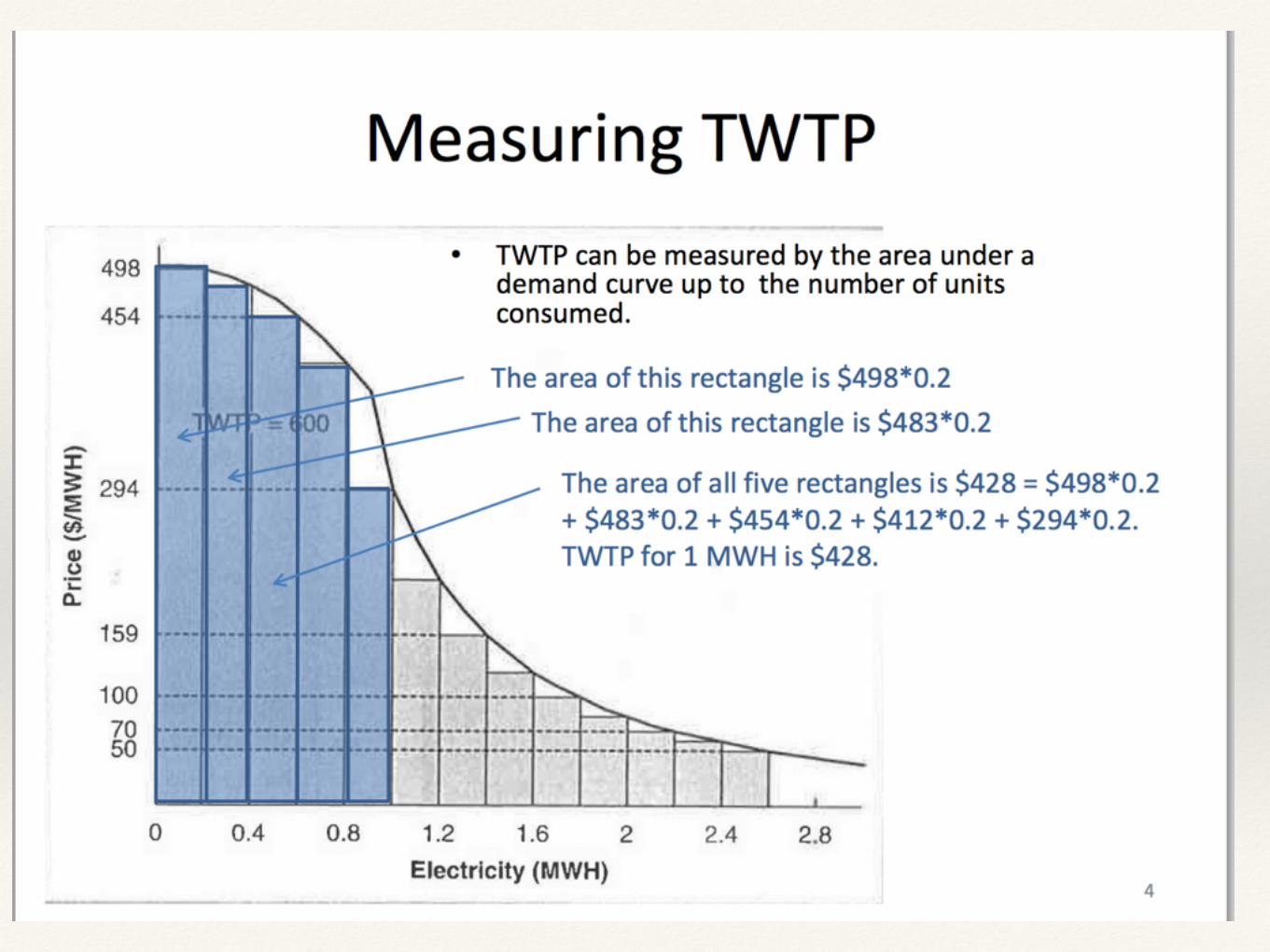
❖ Lets say our demand curve is as follows:!

❖ Electricity = c(0.1, 0.2, 0.4, 0.5, 0.6) MW!

❖ Marginal willingness to pay = c(300,250,200,50, 20) $/MW!

❖ Write a function that takes as input a data frame with values for marginal willingness to pay for different electricity values and returns total willingness to pay for a given electricity requirement (in MW)!

❖ Take as input to the function a data frame called curve that has two columns elect, mwtop (electricity and marginal willingness to pay), and the electricity requirement

Key Programming concepts: Control Structurescompute_TWP = function(curve, req) { !!total = 0 i=1 prev.elect = 0 while (( curve$elect[i] <= req) && (i < length(curve$elect))) { total = total + (curve$elect[i]-prev.elect)*curve$mwtop[i] prev.elect = curve$elect[i] i = i+1 } !return(total) } !!

compute_TWP = function(curve, req) { !!total = 0 i=1 prev.elect = 0 while (( curve$elect[i] <= req) && (i < length(curve$elect))) { total = total + (curve$elect[i]-prev.elect)*curve$mwtop[i] prev.elect = curve$elect[i] i = i+1 } !return(total) } !!> !> example.curve = data.frame(elect = c(0.1,0.2,0.4,0.5,0.6), mwtop=c(300,250,200,50,20))!> example.curve! elect mwtop!1 0.1 300!2 0.2 250!3 0.4 200!4 0.5 50!5 0.6 20!> compute_TWP(example.curve, req=0.2)![1] 55!> (0.1*300)+(0.1*250)![1] 55!>

compute_TWP = function(curve, req) { !!total = 0 i=1 prev.elect = 0 while (( curve$elect[i] <= req) && (i < length(curve$elect))) { total = total + (curve$elect[i]-prev.elect)*curve$mwtop[i] prev.elect = curve$elect[i] i = i+1 } !return(total) } !!

> example.curve! elect mwtop!1 0.1 300!2 0.2 250!3 0.4 200!4 0.5 50!5 0.6 20!> > compute_TWP(example.curve, req=0.7)![1] 100!> compute_TWP(example.curve, req=0.6)![1] 100!> compute_TWP(example.curve, req=0.9)![1] 100!> compute_TWP(example.curve, req=0.3)![1] 55!> compute_TWP(example.curve, req=0.4)![1] 95!> >

Example

❖ If the user asks for an electricity requirement beyond what was described by the demand curve, return NA from the function!

❖ How would you implement thatcompute_TWP = function(curve, req) { !!total = 0 i=1 prev.elect = 0 while (( curve$elect[i] <= req) && (i < length(curve$elect))) { total = total + (curve$elect[i]-prev.elect)*curve$mwtop[i] prev.elect = curve$elect[i] i = i+1 } !return(total) } !!

Examplecompute_TWP = function(curve, req) { !!highest.elect = max(curve$elect) if (req <= highest.elect) { total = 0 i=1 prev.elect = 0 while (( curve$elect[i] <= req) && (i < length(curve$elect))) { total = total + (curve$elect[i]-prev.elect)*curve$mwtop[i] prev.elect = curve$elect[i] i = i+1 } } else { total="NA" } !return(total) } !!!

> example.curve! elect mwtop!1 0.1 300!2 0.2 250!3 0.4 200!4 0.5 50!5 0.6 20!!> !> compute_TWP(example.curve, req=0.4)![1] 95!> compute_TWP(example.curve, req=0.9)![1] "NA"!

Assignment 2

In your group, write a simple function (that involves at least two data types and a control structure) !Enter this function in your organization’s github space! Read/create some data to test your function!Also include that in github!Submit the link the repository!

programing fundamentals - ucsb-bren. · pdf fileprograming fundamentals. modularity main...

Documents