project1 group3

AN ANALYSIS OF THE DONOR-CELL UPWINDING AND CORNER-TRANSPORT UPWINDING METHODS FOR TWO DIMENSIONAL

ADVECTION EQUATIONS

MARCUS N. MORGAN, JAMES S. BROWNLEE, BRYAN P. HOLMAN

Department of Marine and Environmental Systems Florida Institute of Technology, Melbourne, FL

25 February 2014

1. Introduction This paper analyzes the Donor-Cell Upwinding (DCU) and Corner-Transport Upwinding (CTU) scheme’s solutions to the two-dimensional advection equation outlined in equation 1. The goal of this analysis is to determine the more appropriate scheme to use to solve [1]. In order to accomplish this, first the problem statement will be displayed and the DCU and CTU schemes will be presented and discussed. The schemes will then be implemented for the given parameters in the problem statement and analyzed. It will be shown that the spacial and temporal time steps needed to be changed in order to provide a stable solution for both methods. The dissipative qualities of each scheme will be discussed, and then a final determination on the better scheme will be made. 2. Problem Statement

The analysis provided in this paper came from solving the two-dimensional advection equation

qt +uqx + vqy = 0 [1]

with the initial condition

( ) ( ) ( )⎪⎩

⎪⎨⎧ −+−−=0

233.0/5.05.010,,22 yxyxq

if x − 0.5( )2 + y− 0.5( )2 < 0.233otherwise

[2]

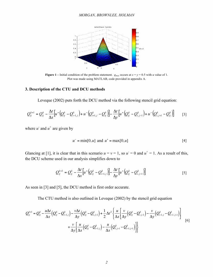
It was given in the problem to use a spacial grid of 64/1=Δ=Δ yx . In addition to that, the time step was set at xt Δ=Δ 8.0 . Here the time step is dependent on the spacial grid in the x direction. Lastly, we were asked to calculate and plot the solution at t =1s and t = 4s. A plot of this initial condition (equation [2]) is shown in Figure 1.

MORGAN, BROWNLEE, HOLMAN

2

Figure 1 – Initial condition of the problem statement. qmax occurs at x = y = 0.5 with a value of 1.

Plot was made using MATLAB, code provided in appendix A.

3. Description of the CTU and DCU methods

Leveque (2002) puts forth the DCU method via the following stencil grid equation:

( ) ( )[ ] ( ) ( )[ ]kijkji

kji

kij

kij

kji

kji

kij

kij

kij QQuQQu

ytQQuQQu

xtQQ −+−

Δ

Δ−−+−

Δ

Δ−= +

−−

++

−−

++1,1,,1,1

1 [3]

where u- and u+ are given by

u− =min[0,u] and u+ =max[0,u] [4]

Glancing at [1], it is clear that in this scenario u = v = 1, so u- = 0 and u+ = 1. As a result of this, the DCU scheme used in our analysis simplifies down to

( )[ ] ( )[ ]kji

kij

kji

kij

kij

kij QQu

ytQQu

xtQQ 1,,1

1−

+−

++ −Δ

Δ−−

Δ

Δ−= [5]

As seen in [3] and [5], the DCU method is first order accurate.

The CTU method is also outlined in Leveque (2002) by the stencil grid equation

Qijk+1 =Qij

k −uΔtΔx

Qijk −Qi−1, j

k( )− vΔtΔy

Qijk −Qi, j−1

k( )+ 12 Δt2 uΔx

vΔy

Qijk −Qi, j−1

k( )− vΔy

Qi−1, jk −Qi−1. j−1

k( )#

$%

&

'(

)*+

+vΔy

uΔx

Qijk −Qi−1, j

k( )− uΔx

Qi, j−1k −Qi−1, j−1

k( )#

$%&

'()*+

[6]


3

This scheme is second order accurate, and is comprised of the DCU plus higher order terms. Due to the given initial conditions, [6] can be simplified to

Qijk+1 =Qij

k −uΔtΔx

Qijk −Qi−1, j

k( )− vΔtΔy

Qijk −Qi, j−1

k( )+ 12ΔtΔx#

$%

&

'(2

2Qkij − 2Q

ki−1, j − 2Q

ki, j−1 + 2Q

ki−1, j−1

)* +,

[7]

As shown in Appendix A, equation [7] was used during the analysis. 4. CTU and DCU solutions

In Figure 2, the DCU and CTU solutions for [1] are shown for time equal to 1 second and

at time equal to 4 seconds. For the DCU method at both times, it is quite clear that the scheme is unstable as the solution to the advection grows without bound. In contrast to this, the solution for the CTU method is stable, although there is damping when this scheme is used. The CTU solution broadens spatially in the xy-direction in order to conserve the volume of the wave as it damps. Therefore, based off the initial condition, the DCU method is computationally unstable, and the CTU method is computationally stable. This is true when the time step is set at 0.8Δx. From here, it will be shown in the following section that when the time step reduced to 0.5Δx, the DCU method becomes stable, and when the time step is increased to 1.1Δx the CTU method becomes unstable.

Figure 2 – DCU method at t = 1 second (upper left) and t = 4 seconds (lower left), as well as the CTU

method at t = 1 second (upper right) and t = 4 seconds (lower right).


4

5. Stable DCU and unstable CTU solutions

According to Leveque (2002), the stability criteria for the DCU method is based on the condition

1≤Δ

Δ+

Δ

Δ

ytv

xtu

[8]

which clarifies why the DCU method was unstable with a time step of 0.8Δx. Because the spacial grid used in the problem is the same in the x and y direction, [8] yields a stable condition for the DCU only when Δt ≤ 0.5Δx.

In the same text, the stability criterion for the CTU method is based on the condition

1,max ≤⎟⎟⎠

⎞⎜⎜⎝

⎛

Δ

Δ

Δ

Δ

ytv

xtu [9]

meaning that the CTU solution becomes unstable in the scope of this problem when the time step is increased to anything larger than Δx. Figure 3 shows the DCU and CTU methods for the DCU-stable time step of 0.5Δx and the CTU-unstable time step of 1.1Δx.

Figure 3 – Plotting of the DCU solution to equation [1] with Δt = 0.5Δx (left) to show how the DCU method

behaves under stable conditions and similarly the CTU method with Δt = 1.1Δx (at right) to show how the method performs under an unstable time step.

To summarize, the DCU becomes computationally stable at smaller time steps, and the

CTU method is able to have a larger time step than the DCU method (because of their respective stability conditions) and still provide a reasonable solution to [1]. At this point it can be concluded that in order to provide a stable solution to the advection equation, the DCU method is more computationally expensive, since it requires a smaller time step.


5

6. Wave damping analysis

This section analyzes the behavior of the solution for each method under stable conditions to determine which method more accurately solves the advection equation. In Figure 4 below, the damping of the CTU solution at t = 1 and t = 4 seconds with a times step of 0.8Δx is shown. These plots were created by taking the initial condition (Figure 1) and subtracting the CTU solution from it. This analysis shows that after one second the amplitude, originally with a value of q(x,y) = 1, has damped by 30% after one second and by 58% after four seconds.

Figure 4 – Plot of initial condition minus the CTU solution at t = 1 second (left) and t = 4 seconds (right).

This plot shows the continual dissipation in the solution as time increases. It should be noted that while this dissipation is significant, the DCU method did not provide a stable solution with the given Δt = 0.5Δx.

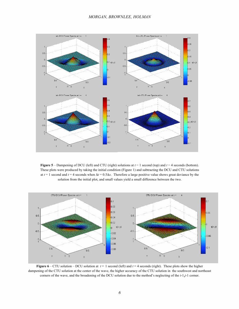
In Figure 5, a comparison is made about wave damping between the DCU and CTU

methods at time = 1 and 4 seconds when Δt = 0.5Δx so that both methods yield stable solutions. At time of 1 second, the DCU solution damps 41% and the CTU method damps 47%. At time of 4 seconds, the DCU method damps 63% and the CTU method damps 75%. Overall, the CTU method damps slightly faster than the DCU for this time step, and damps much quicker than the CTU method when Δt = 0.8Δx. Therefore, the smaller the time step, the more dissipation becomes an issue that inhibits the accuracy of the solution for the CTU method.

In Figure 6, the damping rates are compared between the CTU method and the DCU method by subtracting the DCU solution from the CTU solution. At both t of 1 second and t of 4 seconds there is a negative depression from the northwest quadrant to the southeast quadrant of the wave because the DCU solution damps more slowly than the CTU solution at the center of the wave. In other words, the DCU solution values remain higher than the CTU solution. However, the CTU solution has a higher value in the northeast and the southwest quadrants of the wave because the DCU method does not take into account the Qi-1,j-1 cell, while the CTU method does. In other words, the stable CTU solution is a better representation of the initial wave than the DCU solution. The CTU solution maintains the initial wave structure and does not elongate as the DCU solution does.


6

Figure 5 – Dampening of DCU (left) and CTU (right) solutions at t = 1 second (top) and t = 4 seconds (bottom). These plots were produced by taking the initial condition (Figure 1) and subtracting the DCU and CTU solutions at t = 1 second and t = 4 seconds when Δt = 0.5Δx. Therefore a large positive value shows great deviance by the

solution from the initial plot, and small values yield a small difference between the two.

Figure 6 – CTU solution – DCU solution at t = 1 second (left) and t = 4 seconds (right). These plots show the higher dampening of the CTU solution at the center of the wave, the higher accuracy of the CTU solution in the southwest and northeast

corners of the wave, and the broadening of the DCU solution due to the method’s neglecting of the i-1,j-1 corner.


7

7. Conclusion

For the specified parameters of the problem the CTU method provides the better solution of the two schemes. When Δt = 0.8Δx the CTU method is computationally stable, while the DCU method is unstable. If a similar scenario were presented where

1>Δ

Δ

xt

then neither solution would yield reasonable results, as both would be unstable at that point. If the time step were given by the condition

ΔtΔx

≤ 0.5

then the method of choice would still be the CTU method. While the CTU solution does have a higher rate of dissipation than the DCU method at this time step, the geometric structure of the initial wave is preserved in its circular nature, and has a more uniform broadening than the DCU solution does, especially when time is larger. Most importantly, because the CTU method is stable at a larger time step than the DCU method, the CTU method is much less computationally expensive, meaning that solutions for complex advection equations can be done with less expensive processors, or can be done in a smaller amount of time than the DCU method. To conclude, the CTU method more accurately simulates the solution to the advection equation, maintaining both structure and stable damping of the initial conditions. Reference

Leveque, Randall J. Finite Volume Method for Hyperbolic Problems. Cambridge New York:

Cambridge University Press, 2002.


8

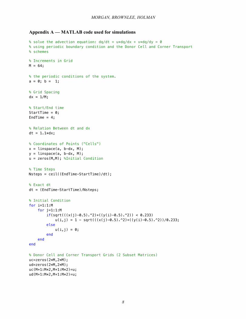
Appendix A — MATLAB code used for simulations

% solve the advection equation: dq/dt + u*dq/dx + v*dq/dy = 0 % using periodic boundary condition and the Donor Cell and Corner Transport % schemes % Increments in Grid M = 64; % the periodic conditions of the system. a = 0; b = 1; % Grid Spacing dx = 1/M; % Start/End time StartTime = 0; EndTime = 4; % Relation Between dt and dx dt = 1.1*dx; % Coordinates of Points ("Cells") x = linspace(a, b-dx, M); y = linspace(a, b-dx, M); u = zeros(M,M); %Initial Condition % Time Steps Nsteps = ceil((EndTime-StartTime)/dt); % Exact dt dt = (EndTime-StartTime)/Nsteps; % Initial Condition for i=1:1:M for j=1:1:M if(sqrt(((x(j)-0.5).^2)+((y(i)-0.5).^2)) < 0.233) u(i,j) = 1 - sqrt(((x(j)-0.5).^2)+((y(i)-0.5).^2))/0.233; else u(i,j) = 0; end end end % Donor Cell and Corner Transport Grids (2 Subset Matrices) uc=zeros(2*M,2*M); ud=zeros(2*M,2*M); uc(M+1:M*2,M+1:M*2)=u; ud(M+1:M*2,M+1:M*2)=u;


9

% Create .mp4 Video from Sequence writerObj = VideoWriter('CTU4_1.1.mp4','MPEG-4'); writerObj.FrameRate = Nsteps/30; %30 sec clip open(writerObj); % Begin Method Calculations for n=1:Nsteps % Calculate DCU and CTU Methods Using Pre-Established Grids for i=2:1:M*2 for j=2:1:M*2 donor(i,j) = ud(i,j)-((dt/dx)*(ud(i,j)-ud(i,j-1)))-((dt/dx)*... (ud(i,j)-ud(i-1,j))); corner(i,j) = uc(i,j)-((dt/dx)*(uc(i,j)-uc(i,j-1)))-((dt/dx)... *(uc(i,j)-uc(i-1,j)))+(((dt/dx).^2)/2)*... (2*uc(i,j)-2*uc(i-1,j)-2*uc(i,j-1)+2*uc(i-1,j-1)); end end % Reset First Subset Matrix to Equal that of the Second for Periodic % Conditions for i=1:1:M for j=1:1:M donor(i,j)=donor(i+M,j+M); corner(i,j)=corner(i+M,j+M); end end % Update Variable for Next Iteration ud = donor; uc = corner; % Print Variables from the First Subset Matrix for i=1:1:M for j=1:1:M donor1(i,j)=donor(i,j); corner1(i,j)=corner(i,j); end end % Simulate set(gcf,'renderer','zbuffer'); surf(x,y,corner1); %zlim([-1 1]); %only if system is stable colorbar('location','eastoutside'); ylabel(colorbar,' q(x,y)','rotation',0); title(['CTU Power Spectra at t =' rats(n/(1/dt))]); xlabel('X'); ylabel('Y'); F= getframe(gcf); writeVideo(writerObj,F); end close(writerObj); clear clc

project1 group3

Science