NSWC!DL TR-3624

00

{ MAP PROJECTION EQUATIONS

byFREDERICK PEARSON I

Warfare Analysis Department

MARCH 1977 ' - .

, ,{)p:nvtd for pLblic rCIC1e,; d.islritUton unhTIilO .

NAVAL SURFACE WAOSCNEDahlgren Laboratoryfahigren, Virqnia 22448

9

NAVAL S1JRFACI, WEAPONS CENTEB"lI)AIill(;RElN LABORATOR(1Y

M. '~ r A i SN

DISCLAIMER NOTICE

THIS DOCUMENT IS BEST QUALITYPRACTICABLE. THE COPY FURNISHEDTO DTIC CONTAINED A SIGNIFICANTNUMBER OF PAGES WHICH DO NOTREPRODUCE LEGIBLY.

UNCLASSlIIl1)SECUR~ITY CLASSIPICATION Or- THIS WAGE (When Date FnIaed)

REPORT DOCUMENTATION PAGE HREAD COMTRLETINO

-,REPORT NUMBER .QV CESO O .RCPETSCTLGNME

MAP 'RoWucTioN 1i'QUATIONS 0 ia'~ ~

7,~~~~S ATO4m1,coNTRACT ON GRANT NUMINER(s)

S. 109AFORMIN@ ORGANIZATION NAME AND ADDREI5S Fo %A TPOU TASK

Naval Surface Weapons Center (DK413

LDallreti, Virginia _2^448It, CONTROLLING OFFICE N AME AND ADDRESS r1-4WTD

D~efense Mapping Agency TNWashington, DC 236

14 O EC 1144R1 , IAA f1FF IS SECURITY CLASS, (*I this report)

(I- AbwC 'ii $UNCLASSIFIEDk,,*,*... ~a, ~!k~u~r GW OINO

IF oirrtTRiUINSATMN oiJI Report)

Approved for public release; distribution unlimited ,

1, DlISTRIBUTIN STATEMENT (of the abstract entered In Slook 20, It dille,.nt tromReot U,1

1S. IUPPLIMRNARY NOTES

1S. KEY WORDS (Continue an rev'erse side it noe..**fy and Identity by block number)

Map Projections Differential Geometry*Conformal Mappitig Fi'gure of the Earthi

* * 9ANSTRAC? (Confinue on rev,,. side I $necessary anid denify by block number)

miapping schemeis. The Important unifying principles of differential geomnetry are 'applied toproduce the equal area, conformal and conventional projections. This report has collected

* under one cover the major map projections useful to scientists and engineers. The notationIs unitorni. The derivations proceed in all cases fromn first principles to usable equationssui1table for hiand plotting, digitalfanalog plotting, or CRT display. (see back)

DD A 147 EDITION OF I NOV 61 I1 OBSOLETE UCASFFS/N 0102- LF- 014-6601 SECURITY CI.A9SIPICATION OP THIS PA09 (Wte Vtotoed

3 91 2_ _

SECUflIYY CLASSIFICATIOm OF THIS PAOB (When Data Enfered)

20)

fl obpQbkm is scad, descr iui itouedt h Wiioo ftibe ar amal)pr iections. B3asic transformation theory is introduced, and then particularized for thetrl'rl'llationl from the spheroid or %phvre onto LI developable surfiAce The criterin forthU derivations is to use the most simple Land direct approach,

A.c -iuio ieeri stm osdrd ems eetprmtr odsrb h

figure of' the earth aire given, and tables Incorporating these are Included for meridianlength, parallel length and the relation between geodetic and geocentric latitude, Thecomputer priogramsfl which goterated these tables aire included in the appendix,

Ikiuui area, conformal, and convenltional projection equations are derived. These Cquations111r 'Incorporated into an1 originial computer progruii which generated the map plotting tablesI'&~ the most Important projections. This program, which produces either a complete grid orindiividualiz~ed Points, is also In thle appendix. Since the proof of all of the derivations is itcorrect graticule of meridians Land parallels, original figures of these have been produced,fhc: plotting tables and the figurvs reflect, the modern parameters for the earth.

The critcrion Vor (lhe success of an!, projection scheme, and the tool for selecting thevmo1st us~eful SQiIL'n1e Imin and application Is obtained by considering the theory of disturtil i.A Iunlericil method is introduicd which permits a quantitative estimate of linear' midunIguIlain distortion,

S N 0 102- IA 0 )1.661 NlSlll)

strUMITY CLASSIFICATION OF THIS PAOEf"Otba fore t.d)

FOREWORD

This report derives the mapping equations for the majority of map projectionsin current use, based on the unifying principles of differential geometry, Thepublication of this report was sponsored by the Defense Mapping Agency,Washington, D.C.

This report has been reviewed by Mr, R, J, Anderle, Head, Astroniautics andGeodesy Division and Dr. Leonard Merrovitch, ESM Advisor, VPI & SU.

Released by:

O .nM a daWarfare Analysis Department

. .

i ] I l, i .

.............................. . .

ACKNOWLEDGEMENTS

My thanks go to Mr, Richard J. Anderie, NSWC, andDr. Alvin V. I lershey, NSW, for review and criticism, and to

Mr, Raymond B. Manriquv, NSWC, and Mr. Kenneth Nelson,

*DMA, For making Information available,

My thanks and the dedication go to my wife Betty,

ai'on

TABLE OF CONTENTS

Chapte'r Page

1 INTRODUCTION ........................ *..... .1

IJ Introduction to tile Problem ....................1.2 Distortion ............... *..........*........ 21.3 C'oordinate Systems ............ *............... 41

1.4 Scale . .....................................

1.5 Classification by Feature Preserved ............... 71 .6 ClasMifieat11il by Projection Surfaice ............... 81.7 Classiflication by Orientation of Azinluth Planle ...... 121.8 C'lassilietIon ot OC 1n and Cylinder *............. 141.9 Projection Techniques ......................... 14

1.11 Comiputer 1iilnentatiln .................... 19

21 MAPP~ING TRANSITORMATIONS .................... 20

2.1 Differential Geometry of Curves ............... 202.2 lDill'orential Geometry o1' Surfaces ................ 302.3 First Fundamental Form ....................... 322.4 Second Fundamental Form ..................... 352.5 Surfaces of Revolution........................ 41

26 Developable Surfaces .......................... 482.7 1'raisformtIon Matrix . . . . . . . . . . . .. 50

8S Conditions of Equal Area and Conformiality ..... 572.9 (Convergence of'the Meridians .......... 571.10 Rotation of' the Coordinate System ................ 61

3 FIGURE 01F TI 1' IVARTIl I ......................... 64

3.1 Geonietry ci the I'llipse ........................ 643. 2 G;eometry of' the Spheroid ...................... 093.3 istances and Angles onl the Spheroid ............. 753.4 Geodetic Spheroids ........................... 873.5 Reduction of' tile Formulas to tile Sphere .......... 9031.6 Figur'e of' the Moon ........................... 95

HIk

Chapter Page

4 EQUAL AREA PROJI:CTIONS ....................... 96

4.1 Authalic LatitUd *............................ 964,1 Conical: One Standard Parallel, Two Standard

Paralle ls ........ ..................... ..... 1014.3 Azimuthal, Polar, Oblique, E.quatorial ............. 1134,4 B onne ..................................... 12 14.5 C'ylindlrical1 ............................ ...... 126

4.6 Sinusoid l ............................. . . . 13 14,7 Mollweide ............ ... . . ... .. . 1354,8 Parabolic ...... . . ............ .......... 1424.9 1 m e -A itoff ,.............................. 147

4,10 Interrupted ..... .. . .. .......... .... ..... 1524,11 W erner ..................................... 1564.12 lEum orphic .................................. 158 ']

4,13 Eckert ..... ............... 160

5 CONFORMAL PROJ FCTIONS ....................... 163

5.1 The Cunformal Sphere ... ........... .. 1035.2 Mercator; Equatorial, Oblique, Transverse .......... 1715.3 Lambert Conformal; One Standard Parallel, Two

Standard Parallels . ............. 1835.4 Stureographc; Polar, Oblique, Equatorial .......... 195

6 CONVI'NTIONAL PROJECTIONS .................. 205

6. 1 Gnomonlc, Polar, Oblique, Equatorial ............. 2056.2 Azimuthal Equidistant; Oblique, Polar ............ 2156.3 OrthographIc; Polar, Equatorial .................. 2226.4 SImple Conic; One Standard Parallel, Two Standard '1

Parallels, Perspective ....................... 2296.5 llolyconic Regular, Transverse .................. 2416.6 Simple Cylindrical, Perspective, Miller ... ......... 245 '16.7 Plate C rr&' ................................. 2496.8 Carte Parallclogrammatiqcue ..................... 2506.9 (Ilo btilar ... .... .. ...... .... ....... .. ....... .2 5 1 '6 .10 0 all ... ... .. ... .. .. .. ..... ...... ....... .... 2 55 {

6.11 V ad tier G rinten ............................. 257(1. 12 M urdoch ................................... 251)6.13 StereographIc Variations1 -Clarke, .James, La I lIre ..... 2626 .14 C assint ..................................... 266f i

iv

r|

('11 ipte r Pg

7 THEORY OF DISTORTIONS ................. ...... 268

7.1 Distortion in Length .......................... 2687.2 Distortion in Angle ........................... 2697,3 Distortion in Area ...... ................ ...... 2727.4 Distortion in Equal Area Projections .............. 2737,5 Distortion in Conformal Projections ........ ..... 2767.6 Distortion In Conventional Projections ............ 2787.7 Qualitative Comparisons ....................... 279

8 CO NCLUSI N . ................................... 285

APPENDIX

A.I PROGRAM MAP .................................. 289

A.2 ANCILLARY PROGRAMS .......................... 325

vI

. ... .I l i

FIGURES

Figure Title Page

1.2.1 Distortion Ft'fects ............................... 3I

1.3.1 Terestral. oordinato System ........ ...............1 .3.2 Map Coordinate System ............................. (I1.511 Quadrilateral liepresentation .. .. . .. .. . ..... . .. . .. .. .. 9

1.6.2 C'one Tangent to the Earth ............... I I16.3 C'one Secant to the lEarth ................. ,...... 131.71 Orientation or' thle Azimutthal Plane .................... 15I1.8.1 Orientation ol'a Cylind.er,.......................... 16I ..I Graphical Projection Onto a Plane ........... 171.10.1 Azimuth of' W from P ....... ,............ 18

2.1 Geometry of' a Space Curve .......... ,........ 212.1.2 consecutive rangent Vectors ........................ 212. 13 Pl1anes onl the SpacQ Curve at Point P ....... 252.2.1 I'la I'lHMtHC Cuirves ., ........ ,.......,... , 11

I.. Geometry for a Surface of Revolution .. ....... 42

2.7.1 Parametric Representation of' Point P1 onl the E 'arth ........ $1

2.,2 Parametric Representation or point I" onl the projection

2.9.1 Geometry for the Angular Convergence of' thle Meridians. ... 592.9.2 Geometry f'or Linear Convergence or' the Meridians ..... 601.10,1 Geometry for thle Rotational Transformation ...... 6 23. 11 Geometry of the ElIlipse . . . .. . . . . .. . . . . 65

3. 2.1 Geometry of'the Spheroid .............. ..... 703.3.1 The Azimuth of,;~ Curve...... ............ 833.3.2 D~ifferential Element IC1ellnlng I Rhunibline onl a Spheroid , 863.5.1 Gjeometry of' thle Sm.h....... r....... 913.5.2 Distance Between Arbitrary Points on a Spere ......... 933.5.3 D~ifferential Filement Deflliing a hu~mbline onl the Sphere 944.1.1 Conical Equal Area Projection, One Standard Parallel .... 1064. 2.2 Conical Equal Area Plrojcvtion. Trwo Standard Parallels ... 1094.3.1I AziI.imthal liqual Area Projection. Polar' Case ............ 1154.3.2 Azimuthal Uqual Area Projection, Oblique Case ...... 1194,3,3 Azimu1.thal Eqkual Area Projection, Equatorial Case ..... 1204.4.1 Bonne Equal Area Plrojectionl .. ,...................... 1254.5.1 Cylindrical Eqjual Area Projection ........... 1294.6.1 Sinusoidl Projection ,,..,.................. 1 334.7.1 Geometry for the Mollweide Plrojection .......... 1 364.7.2 0 vs 0 for the Moliwelde Projection .......... 1 384.7.3 Mollwelde Projection ........................ 14a4.8.1 Parabolic Projection ..... ,................ 1434.8.2 Geometry for the Parabolic Projection ........ 1444.9.1 1 lammer-Altoll' Projection ............. . 1484.9.2 Geometry for the I lmmner-AitolI' Projection ....... 14()

vi

I 'ILINr lit IC Page

4,10. 1 Interrupted Sinusoridal Projection .................... . 1534,10.2 Interrupted Mollweide Projection .............. ....... 1544,10.3 Interrupted Parabolic ProJection ..... ......... . . . 1554.11.1 Werner's Projection ".............. ....... .... . 1574,1'21 IFumorphic Projection .............................. 1594.13.1 Gcom .try for Ichert's Projection ...... ............... 1615,2.1 The Varying Projection Point .for the Mercator Projection, , . 1725,2,2 IR.egular, or i'latoril Mercator Projection ............. 175

5.2.3 Oblique Mercator Projection ...................... 1765.2.4 Transverse Mercator Projection' . ....................... 1775.3.1 Lambert Conlormal Projection, One Standard Parall ...... 1845.3.2 Lumbert ('onformal Projection, irwo Standard Parallels..... 1935.4.1 Geometry of the Stereographic Projection ............... 1965.4.2 Stereographic Projection, Polar Case .. ................ 1985.4.3 Stereographic Projection, Oblique use ................. 2015,4,4 Stereographic Projection, Fquatorhd Case ............... 2036.1, I (;eometry of the Oblique Gnomonl& Projecton ........... 2066.1.2 Gnomonlc Projectlon, Oblique Case .................... 2096. 1.3 Gnomonic Prolection, Polar Case ,,.,,......... . 2116.1.4 Gnomonic Prv.lection, Equatorial Cse .................. 2136.2,1 Geometry loi the Oblique Azimuthal [I'quldistant Projection, 2166,2,2 Azimuthal Equidistant Projection, Oblijue Case .......... 2176.2.3 Azimuthal l.quidistant Projection, lPolur Case ............ 2206,3,1 (eometry of the Oblique Orthographic IProjection ........ 2236,3,2 Orthographic Projection, Polar (.use .... ............... 2246,3.3 Orthographic ProJection, Equatorial Case \ ............... 2276,4,1 Geometry for the Simple Conical Projectln With One

Standard Parallel ..................... ........... 2306.4.2 Simple Conical Projection, One Standard Parallel ......... 2316,4,3 Geometry for the Simple Conical Projecton',Wlth Two

Standard Parallels .................... . ............ 2336,4.4 Simple Conical Proijection, Two Standard Par llels ........ 2366,4.5 Geometry for the Perspective Conical Projection .......... 2386.4.6 Perspective ('onical Projection ............ ... ...... 2406.5.1 Regular Polyconic Prolection ...................... 2426.5.2 Traisveie Polyconic Projection ........ ... ....... 2446.6.1 Perspective Cylind riCul Proj1ction ..... . . ..... . 2466.6.2 Millet' Cylindrical Projection ............... .......... 2476.7.1 Plate C'arrdc Projection ,......... ... , .......... 2496.8.1 Carte Iuallelograimatique Projec tion ....... ......... 250 I6,q,1 Geometry for the Globular Projection ........ I ......... 2526,9.2 Globular Projection ................................ 2546,10.1 G all's Projection ................................... 2566.11.1 Van d ir c;rinten's Projection ......................... 2586.12. 1 (eometry of Murdoch's Projection .................... 2606, 13.1 Proiection Points for the Varitions of the Stereographic

Projection ........................... ...... ...... 263

vii

. .

. . ... .....

1 igu re Ttle Page

6.13.2 Geometry ror the Stereographic Variations .............. 2646. 14.1 Casslni's Projection ............ ..... ......... .. . 2677.2.1 l)ifferential Parallelogram ........................... 2707.7.1 Comparison of Azimuthal Projections .................. 2807.7.2 Comparison or Iqual Area World Maps ................ 2827,7.3 Comparison of Cylindrical lProjiections .................. 2837,7.4 Comparison of Conical Projections .................... 284

TABLES

Table Title Page

3.1.1 Geocentric and Geodetic Latitudes .................... o83.2.1 Radii as a ['unction Latitude ......................... 743.3.1 Distance Along the Circle of Parallel for a Separation of I' 763.3.2 Distance Along the Meridianal Ellipse for a Separation of1 1 803.4.1 R'ference. Splheroids .......... ............... 883.4.2 Powers of e for the WGS-72 Spheroid ................ 893,6,1 ,Lu'r Spheroid ....................... 954, 1, I Authalic and Geodetic hititudes ...................... I004.. I Conical Equal Area Projection, One Standard Parallel ...... 1054.2.2 Conical Eiqul Area Projection, Two Standard Parallels ..... 1104,3,1 Azimuthal E-qual Area Projection, Polar Case ............. 1144.3.2 Azimutlal lEqual Area Projection, Oblique Case .......... 11'74,3,3 Azimuthal Equal Area Projection, Equatorial Case ....... 1184,4,1 Bonne Equal Area Projection ................... .... 1244.5.1 ('ylindrical IEqual Area Proiectlon ..................... 1304.6.1 Sinusoidal Projection ............................... 1344.7.1 4ollwelde Projection ............................... 14 14,8.1 Parabolic Projectlon ................................ 1464,9, 1 l1am mer-Aitlofl' Pro.ection ......................... 1514.12.1 Parallel Spacing f'or the l.umorphi c Proiecti O i ............ 1585.1 .1 'onformall Latitude as, a I 1uitiO1i of(Geode tic I.Atitilde for

the W GS-72 Spheroid ............................... 1705.21 Etquatoral Mercator Projction ....................... 1785.2.2 Oblikue Mercator Projection ....................... 1795.2.3 'l'ransverse Mercator Projection ..................... 1805.3,1 Lambert Con formal Projection, One Standard Parallel ..... 189)5.3.2 Lambert Conformal Projection, Two Stanlard I'arallls ... ,. 1945.4.1 Stereographic Projection, Polar Case ...... ............. I ()L5.4.2 Stereographic Projection, Oblique Case ................. 2025.4.3 Stereographic Projectionl, [q uatorial 'ase ............... 2046.1.1 (nomonlc ProJection. Oblique Case ................ 2106.1.2 ( noinonic Projection, Polar Case .......... ....... ..... 212o.1.3 (;0notuonic Projection, IltquatoMrlal Case .................. 214

viii

la hI e Tile Page

6.2,1 Azimuthal Equidistant Projection, Obliquc Case ...... 2186.2.2. Azimuthal Equidistant Projection, Polar Case .......... 2216.3. 1 Orthographic Projection, Polar Case ................... 2256.3.2 Orthographic Projection, Eqtvatorial Case.............. 2286.4.1 Simple Conical Projection, One Standard Parallel ..... 2326.4.2 Simple Conical Projection, Two Standard Parallels ........ 2376.5.1 Regular Polyconic Projection ........... ,........... 2436.6.1 Simple Cylindrical Projection ...... ,.....,........... 248

ix

Chapter I

INTRODUCTION

Map projection is the orderly transfer of positions of places onl the surface of thle earthto corresponding points on a flat sheet of paper, a map. The process of transformation re-quires a degree of approximation and simplification, This first chapter lays the grotind-workI'm the study by detailing, in u qualitative way, the basic problem and Introducing the ;nomenclature of maps, Succeeding chapters will consider thle mathematical techniques andthe simplifications required to obtain manageable solutions 191 ,*

All projections Introduce distortions in the maup. The types of distortion aire consideredIn terms of length, aingle, ;ind area. This chapter discusses the qualitative aspects of the prob)-tern, while Chapter 7 deals with it quantitatively.

The coordinate systems useful in locating positions on the earth, and on the map tiresumllmarized. The concept of scale factor to reduce earth sized lengths to map sized lengthsIs discussed.

Map projections mlay be classified In a number of ways, The principle Oo is by thlefeatures preserved 1'rom distortion by thiv mapping technique. Other method0(s fot LaS4iliCUation depend onl thle plottitlg surface employed, thle method of contact of this surf~cu withthe earth, and thle orientation of thle pliottinlg surface with respect to the direction or theearth's polar axis, Finally, maps can be classified accordinlg to whether or not a map can bedrawn by purely graphical mevans.

The convention forUaMith Used In this Volum111 IS also introduced.

1. 1 iroduction to tile Problem

Map pro~Jection requires the transformiation of' positions from a curved suirface, theearth, onto a plane surface, thle map, ini an orderly f'ashion. Th'Ie problem occurs beause ofthle di t'1ereneec in the suirfaces Involved,

The model of' thle earth is either a spte ro ort spheroid (Chapter 3). These curved suir-facOs hlave two finite radii of curvatte. Thie map11 is a 11la11e surface, mid a plane is cluiractviized by two il'inite radii of cuirvature. As will he shown In Chapter 2, it is impossible totransform from a surface of' two finite radii of curvature to a suirtaLce oh' two in II ite radii ofI

curvature without introducing some1 dlistorttion. The sphere and the spheroid are calleki

* Numbelirs in hnia kec te ~l'vr ti~ i' lhu, '11111p piy.

2

nondevelopable surfaces, This refers to the inability of these surfaces to be developed (i.e,,transformed) into a plane in a distortion free manner [81.

Intermediate between the nondevelopable sphere and tile spheroid, and the plane aresurfaces with one finite and one infinite radius of curvature, The examples of this type offigure are the cylinder and the cone, These surfaces are called developable, Both the cyl-Inder and the cone can be cut, and then developed (essentially unrolled along the finiteradius or curvature) to form a plane, This development introduces no distortion, and thus,these figures may be used as intermediate plotting surfaces between the sphere and spheroid,and the plane. However, in any transformation from the sphere or spheroid to the develop-able surface, the damage has already been done, The transformation from tile nondevelop-able to the developable surface has already introduced some degree of distortion,

Consider of what an ideal map would consist [81.(I) Areas on the map would maintain correct proportion to areas on the earth,

(2) Distances on the map would remain in true scale,(3) Directions and angles on the map would remain true,(4) Shapes on the map would be the same as on the earth,

The Impossibility of a distortion free transformation from the nondevelopable surfaceto the plane prevents the realization of the ideal. The best a cartographer can hope for Is arealization of one or two of these feltures over the entire map. The other features aresubject to distortion, but hopefully to a controlled extent.

The projections of Chapters 4, 5, and 6 are the cartographer's answers to the problems,In each of these projections, sonie of the desired features are maintained, The distortion inthe other features will be tolerable,

1.2 Distortions 1221

)istortion is the villain otf tile piece. Distortion in maps may be in area, lengti, angle,or shalpe,

l)istortion in area is shown in Figure 1.2.1 (-. While shape is maintained, the ilrcal onthe map may be enlarged or diminished,

Distortion in length is com mon, and Fi7gure 1,2, I (h) is an illustration, Often, while thecartographer is able to maintain true length in one direction, he cannot do so it a seolnddirection,

Aingular distortion Is also prevalent, Thlus, angles on a map will not necessarily be thesame as their cotmntcrparts on the earth. Thus, azinuths On the nap, (Y' will notl coincidewith true Izimutls' On the earth, This is shown iln ligure 1.2. 1(c),

)istortion In shape can occur in a t Liiiher of ways, Onc is a gencral change of sliipe ol'the ligue. A second is a shearing type of effect, FIigure I .2. l(d) demostrates both ofthese changes.

(In) Area

(b) Length

ja) Angle

General $hear

(d) Shope

Figure 1.2.1, Distortion effects

4

An actual map will have combinations of these distortions. The numerical theory ofdistortion will be presented in Chapter 7 of this report,

Now that we are acquainted with the problem, the next sections in this chapter willintroduce some of the terms needed for the study of map projections before entering themathematics of Chapter 2.

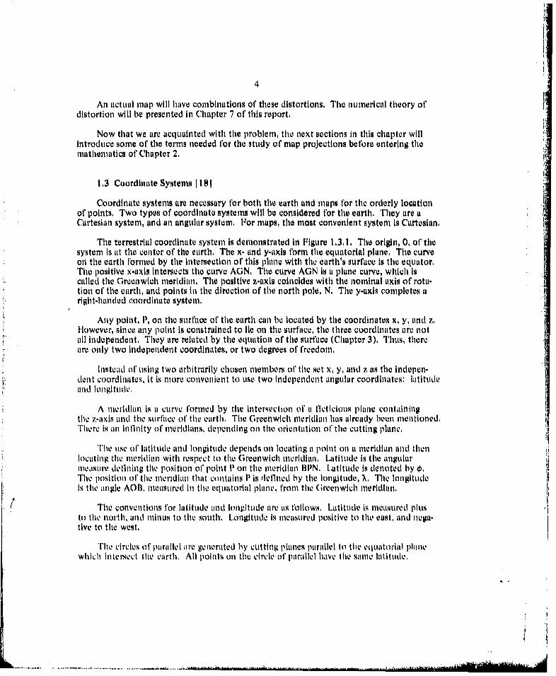
1.3 Coordinate Systems [ 18 I

Coordinate systems are necessary for both the earth and maps for the orderly locationof points. Two types of coordinate systems will be considered for the earth. They are aCartesian system, and an angular system. For maps, the most convenient system is Cartesian,

The terrestrial coordinate system is demonstrated in Figure 1,3,1, The origin, 0, of thesystem is at the center of the earth. The x- and y-axis form the equatorial plane. The curveon the earth formed by the intersection of this plane with the earth's surface is the equator,The positive x-axis Intersects the curve AGN, The curve AGN is a plane curve, which Iscalled the Greenwich meridian. The positive z-axis coincides with the nominal axis of rota-tion of the earth, and points in the direction of the north pole, N. The y-axis completes aright-handed ooordinate system,

Any point, P, on the surface of the earth can be located by the coordinates x, y, and z,However, since any point is constrained to lie on the surface, the three coordinates are notall independent, They are related by the equation of the surface (Chapter 3), Thus, thereare only two Independent coordinates, or two degrees of freedom,

Instead ot using two arbitrarily chosen member, o1' the set x, y, and z as the Indepen-dent coordinates, it is more convenient to use two Independent angular coordinates: latitudeand longitude,

A neridian is i curve formed by the intersection of a l'icticious plane containingthe z-axis and the surface of the earth. The Greenwich meridian has already been mentioned,There is an in filnity of meridians, depending on the orientation of the cutting plane,

The use of ltitude and longitude depends on locating it point on a meridian and thenlocating the meridian with respect to the Greenwich meridian, Latitude is the angularmeasure dehiling the position 01' point P on the merldian 13PN, Latitude is denoted by ,The position of the meridian that contains P is rieflned by the longitude, ), The longitudeIs the angle AOI. measured In the equatorial plane, from the Greenwich meridian.

( The conventions for latitude and longitude are as follows. Latitude is measured plusto the north, and minus to the south, Longitude is measured positive to the east, and nega-tive to the west,

'The circles of parallel are generated by cutting planes parallel to the equatorial planewhich inte'sect the earth, All points on the circle of parallel have the sane latitude.

5

P,.

Figure 1.3.1. Terrestrial coordinate lyitem

:1.

6

The mathematical relationships between the polar and Cartesian coordinates, as well asthe definition of the types of latitude is deferred until Chapter 3, where the sphere and thespheroid are discussed.

The coordinate system for the map, Figure 1.3.2, Is a two dimensional Cartesian system,The plus x-axis is toward the east, and the plus y-axis is toward tle north. The origin, 0', ofthe system will depend on the scheme of projection to be developed in Chapters 4, 5, and 6,In most cases there will be some straight, arbitrarily chosen central meridian which serves asthe ordinate of the projection.

The object of map projection Is to transform from the terrestrial angular system to themap Cartesian system. Chapters 4, 5, and 6 will provide the methods for these transformations.

North

CentralMeridian

S Origin, 0'

East

Figure 1.3.2, Map aoordinate system

7

1.4 Settle 1811

Th'ie sce. ot' th., impl is thle ratio ot' the distance oil tile map11 to the corresponidingp (us-tance oin thv earth, or dmt/do. I I thle distance Onl both hie mlapl and the earth have thle sai meunlits, t hen tile scale Is at di menlsioniless quantity. Seale is another aspect of' the orderlytrans formation from earth measurement to map measurement.

The presence of' distortion requires thle definition of' two types Or' scatle: thle prinlcilelScale and thev local Scale.

The princi ple scale Is base~d onl a meridian or patrallel which is a uniflormily true scale forthle entire ma p. It is thle scale. used for shriniking tilt Spheroidal surfacee of' the carthI to theplane~L of' the0 papllo.

At other places onl thle map, where distortions arc present, thle scale will [it di ffe tntfroil trueo scale. This local Scale will he larger or Smaller than thle prinelial Scale, depenldingonl thev nieclinisni of' thle distortion.

The local Scatle, ats a function of' distort ion, and tile prinlciple scttle mlay be qulotel onIthe legend of a map, A more useful means is a graphical scale drawn i thle map) legend, andspeiM1led lot' tile laItitudeS aind longitudes where it applies. As ant exam~ple, for thie Mercatorproicet ionl ((lliptci 5), a set of scales canl be drawn as a f'un et on ot' 141titudo, which will oin.Sure, the correct distances fIm measuring,

Teterms large scale Versus smlall Scale conicV fro011 consWidertionl 0' thle fractionl d in/LieA scale of' I /10,000 Is a large scatle, and I1/ 1000,000 Is at small scale. A plan, or it mup Show-lu19 baldiligs, cutlt url features, or boundaries IS USulI/II 1/0,000) ort larger. A topographi c1111) p.Which gives roads, railroads, towns, and contour lines, and othler' details ins a1 seatle lie-twee it I / 10,000 atnd I / I 000,000. Maps of' a Scale smit 11cr Ihanl I/I 1,000,00() tire at las maps.Ihse lmps Li Ilnate cowl tries, continents. and~ oceanls

lThe scalt. I'actor, S, I iso Iselli the plotting equations of' Chapters 4, 5 and fi, and isOqual to din/dc.

1.5 ('lassiflenlun by Fecature, Preserved 1 21

Matps Ilay lie classified by thle fea1ture tescuedl front (istortilt, or bly file agreentientthat Some dhistort ion will Simply tie tolerated, Thfis system of' classification Lilvides mapsInto Ilivrv. Catagoriles: equal itreai. conflottual aid Conventional.

Thv eqpual areal projoctioll l'resoives thle ratio of areas onl the earth and onl thle lmp as a~onlstant. Aniy part tit' thle map 11ear1S tile S411110 relation tLI tile areal onl t11e odtth it rehlireSWets

that the Whole map11 bear's to thet total earth area represented. Any quadlrangtiar shaped Svc-tiOll o1f the 1111111 toI'01L1dII tyi grild of, iietidianls and parallels will beL equail Inl area01 to any of herqilLI1drailgillil area of,11 th same1L Imap that represen,1ts anl equal atrea oft thle 'arth Angles uisuaillysulIfer. A con fractionl ot, ilieridiallis will have to bhoffe hy al leugi liviing of1 parallels, orvice versa., bult the enlclosecl areal Will I0ilit1li the SM111C. 'Tis con1cept is iIIllltratd inl Figlre1.5, I al). All of' the qilaidrilaterals hoive the same area.

A con f'ormal proIlection is one iII which thle shaple ot any silliII su rface of' tile nIap~ ispreserved InI its original form. C'are Must ble used fin applying this concept, since it is trueonly locally, and cannot be extended over large surface areas. The true condition for at con-Formal mall is that thle scale Lit any point Is the saime in aill directions. The scale will changefrom point to point, but it will be Independent of the azimuth tit aill points, The settle willbe tile samec In till directions from at point ii two directions ait right angles onl the earth Liremapped into two directions that aire also ait right angles to eaceh other. The oeridians aindparallels of thle earth Intersect ait right aingles, and at conformal proqJection preserves thisquality onl the matp. Cionformal quadrilaterals aire shown fin l-Igure 1 .5.1 (b). Another termused iII refering to conformal projections is ort'oinorphic, or samex form,

Conventional projections aire all those which aire neither equal area niiotconformial.This is not meant as at disparaging term, Many of' thle conventiontil maps arv of great utility.In tthe Ginomonic projection, the feature preserved Is tlImt great circles become straight lines.Inl the Aihmutlial equidistan t projecion thle distance and azimuthI from thle origina to anyother point onl thle map is true. The lPolyc -),!-and van der (irinteti projections have seenconsiderable ser-vice as road maps. All tl i, is implied by the t':rm conventional is that thecartographter has been willing to isafcvtc t hu fLatures of eq ual area oir con lormalit y inl order

7F to retain some other fe0ature, or to obtain at simple, utilitarian ailgorithm for the projection,

1,06 Chasiication by rojcction Surface 1 221

Only three projetion surf'aces will be conside red -the plane. the conec, and the cylindler,* All pr(~ections inl use today are, accomplished through these, or mlodil'hcationls of' t hese. It*canl be argued that aill projection surfl es aire conlical. since thle plan11e and thle Cylinder canI be

Considered as the two limiting Cases of' the colie. Ilowever, this ma 1theiatical nicety Is notuisual ly used, and thle threce surfaces will be conside red ats di1stinct. in most eases. F igure Lo.61shows each of these surfaces in relation to thle sphere.

Thew ilantir projection surt aice can be used f'or 0 direct t ransf~ormat ion from the eairth,Thev projections which result tire called az.11imthal ( I igure 1.0, 1 (t) ). 0Other nlamles Ill Ime are-zonitlitl, or planar projections,

Conical projectionls result wheni a cotie is ulsed as mli in toriediate plotting surlfiave. Theconec Is then developed In to a plane to obtainl thle map11 (I Figir 1 .0 61(11)).

At this point It Is convenienit to Introducve thle conlcept of' the Const antI of' t li conec. I vta hie thle radiuis oft the earth, From Figitre0 1.0.:, the0 slant height of' 11t conec tangent to tileearth, P. Is founld to bie

p --- a Cot 0 11

where 0 Is the latitude. Also, from the figure, d, the lenigth of the parallel ciche Ali, whichdvi'ties tilie circle of' tangenlcy oh thle cone, Is

(I .2ira cos ~ 12

9IIA

(a) Equal area quadrlterals

(b) Conformial quadrilaterals

Figure 1.5.1, Quadrilateral representation

00 10

-. (a) Azimuthal

IA

- N (b) Conical

PI

- - (a) Cylindrical

Figure 1.0.1. Classification by projection surfool

1Ia

I

p

N

A S

*

*0

SPluve 1.6,2, Con. tanpnt to the eaflh

I~r~fl.~ilm.% w.1I El a - -

The constant of the conec, C, Is det'ined l'rom tile retIntionl between thle developed colicanid the earth. Let,

0 = /P. (1.6.3)

Substitute (1.6 1) and (1.6.2) Into (1.6.3)

o 2ira co", 0

o 21r sin. (1.6.4)

The constant of, thle ;,one is c =sin I It is at multiplicative f'actor that relates longi tudes onthe earth to thosec onl the conic. h(JUat ions (1,6,1) and ( 1.6.4) will be beneficial lIn Chapters,4, 5, and 6 lin the investigation of thle various Conicail projections,

'The cone may also be secant to the earth. This Is shown in Figure 1,6.3, where thecircles ol' secancy tire it the latituide' 01 , and 02 . From the similar triangles, thle ratios (it'the slant heights of' these respective latitudes itre

it _ Cos 0

P va os 01

Note lin equation (1.6.4) that ats 0 varies from 00 to 900, 0 varies fromh 0" to 3600,When 0 is 0', then we hatve at cylinder. At 0 equalis 3600, we have a plane. As was menl-tioned above, It will be usefuil, usu~ally, to treat planes, conec, and cylinders as separate en-titles, rather tham lump them together in at single general approach to the prohlem,

Cylindrical projections aire obtained when it cylinder is used as the intermediate plottingsurfface (igure 1.6.1 (c)). As wvith the conec, the cylinder amI~ then be developed into at plane.

lIn Figure 1 .0. I , at represenltativu position Onl the en rth.l, ,Is Shown tranlstormed Into aposition onl the projection suirlace, I" for each (if' the projection suirfaces, Chapters 4, 5, and6 will explain thle methods tha t will affect such transf'ormations, and produce uselul mnaps.

1. 7, Classlifiation by Orientation of (lie Azimuthal Plane 1 221

As was seen fin thle prcvluti section, thle op1tion ol' Using at tangenlt coneC Or at scaLnt Conecis at ieans of' further diffelrentiating conical projections, Similarly, a7ilnLIhl I projectionsmay be clasmi lied by refecrence: to the point of contact of' the plotting surl'aco with the earth,

A,.inithul~l project ions may bie clasiM1L fled a10polar, CLI luitorial, or obliq ue, Wh'~mi the planeIs tange at to thle cL rth at either pole, we have at polar projection, When the laneI is tangenmt

....................... ...

13 I

P1

Figure 1.6.3, Cons s.ent to the earthi

14

to the earth at ally point onl thle equator, the projection is called equatorial, The obliqJuecase occurs when the plane Is tangent at any point on the earth except thle pokus and theequator. F'igure 1.7,1 Indicates these three alternatives. In each case, T is the point of'tangency.

1 . Classification by Orientation of at Cone or Cylinder 1221I

Another classification set canl be defined tfor cones and cylinders. These plotting sur-f'aces may be considered to be regular, transverse, or oblique.

The regular projection occurs when the axis otf the cone or cylinder coincides with thlepolar axis of' the earth. T'he transverse case haus thle axis of' the cone or cylinder perpendicui-lar to, and Intersecting the axis of the earth. The transverse Mercator, and the transversePolyconlic are examples of' this. If' the axis of' the cone or cylinder has anly other position inlspace, besides being coincident with, or perpendicular to, thle axis of the earth, then anloblique projection is generated. Figure 1.8.1 demonstrates these three options for aI simpule

1.*9 Projiection Technitl tic 131 , I II

Three techniques of' projection canl be identified. This canl serve as another scheme o1'classification. The methods are the graphical, the semni-graphical, and the mathematical.

Un an graphicalI tchique(L, Some point 0 Is chosen as a projection point, and thleme~thods ofl pro~ectivo geometry and descriptive geometry are usedi to transform a point 1Ponl thle earth to a location P' onl the plotting surf'ace, An exam ple of' this is Indicated inigure 1.9.1. where thle point 11 onl the earth is transtformed to the oblique plane by thle ex-

tension of' line OP' until It intersects the plane, Inl this example, 0 is arbitrarily chosen astie proJection poinut. Since: an ything that can be done graphically canl also be describedmlathemiaticaIlly, we will not encourage graphical constructions. H owever, t hose lpr(iect ionswhich are capable of' a strict graphical approach will be identifiedI inl Chapters 4, 5, and 6.

Tlhose proiecetions termedQL mathematical will hw those wh i ch canl Only tie produced by amat he maticalI de Ii nition. No dra t'tsmanl with compass and straight edge can plot themi bymeans of' the pro;ection ot a ray.

InI between these two groups are the se mi-graphical project ions. H owever, for variousreaIsons, suich as a varying prqjectionl poinit (Mercator), or a com plex graphical sche mee(M ol we ide), the rcasonlahk' approach is to depend onl a mat hemati cal proceduwe.

1.10 Azimuthi 171

TIhe anlgulat' measiii'e(of' use inl specif'ying directions on the e'arth and on the mapi is f lie,Ailuti. The u/iiuthl ot, I" inl relation to 1P is shown ill FigureI' 1.10. 1 tor the eairth. Azimiutis nicastured m'om thle morth, or the meridian thiough the point 1P. in a clockwise iinilnlrlAzimiuthI is iiiei'surmei the samec way onl the 111a11 as onl thle 0,arth.

15

N

N

N

I (a) Oblique

Figure 1.7.1. Orientation of the azimuthal plane

16

N

(8) Regular

(c) Oblique

Figure 1,.1. Orientation of a cylinder

17

Ph

Figure 1,9.1. Graphical projection onto a plans

181

Figure '1.10.1. Azimuth of P' from P

19

1.1I Computer Implementation

The subject of map projections certainly has intrinsic interest, Of more Importance tosurveyors, cartographers, and all other workers in the field of map projections, is the avail-ability of plotting equations, and their incorporation onto a computer prngram that permitstheir utilization. The ultimate goal of this report is to provide Cartesian plotting equationsas a function of latitude and longitude, and a computer program which includes the mostimportant of them. This will be, at the very least, a good beginning for further practicalwork.

After the basic concepts are derived in Chapters 2 and 3, the actual equations formapping will be developed in Chapters 4, 5, and 6,

The computer program in Appendix A. 1 combines twenty of the most usef'ul mapprojections schemes with the methods of providing equal area and conformal qualities, andthe methods of rotational transformation. In all cases, the latitude and longitude coordi.nates of the earth will be input, and converted into x., and y.plotting coordinates.

These subroutines can be incorporated Into existing and proposed programs, The out-put can be suitable for plotting tables, digitallanalog plotters, or CRT display 1121, [131.

Appendix A, I includes an input guide to the computer program MAP, This will aid theuser In incorporating his values of the earth parameters and scale factor, and selecting therequired projection scheme, The method of selecting a complete grid or a collection ofpoints is also described.

,J ... ,. .. ... . I

Chapter 2

MAPPING TRANSFORMATIONS

The process of' mnp projection requires the transformation fromn the two independentcoordinates of' the eart to the two independent coordinates o1' the map. This chapter willbe devoted to the gene Ija theory of transformations. To this end. it will be necessary todevelop somne applicabli formulas of differential geometry, and apply some aspects ofspherical trigonometry,,

The differential geomnetry of curves will give the needed radius of curvaiture and torsionor' a space curve, The' differential geometry (if surfaces will concern the first int' secondfundamental forms, and parametric curves and the condition of orthogonality, The surlacesoif intrest in mapping are surraces of revolution. The general surt'ace will be particularizedto surfaces of revolution (Chapter 3), The process of transformiation from non-developableto developable surfaces will be considered, Representation of arc length, unglesi, and area,

6 ais well as the defInition of the normal to the surface, will be given.

The basic transformation miatrix will be derived, rhe conditions of equatl area andconforinality will be applied to this transformnation,

rhe convergence otf the meridians is next considered. Finally, a rotation mnethod Iforthe production of equatorial, transverse, and oblique projections will be given,

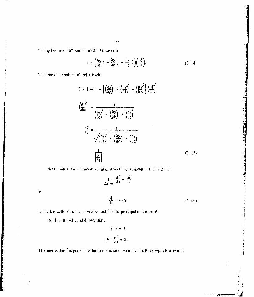
2,1 Differential Geometry of Curve,% 1101

C01nSIder the! spa1ce curve of Figure 2. 1. l. Let b e an airhitrary paramneter, Let thevector to any point 11, on the curve, in the ('artesian coordinate system, be

r =x(O'T + Y(1~ + (21,1

LetII ArI = s.

'111 Liii111 tanigent Vector ait poinit 1) Is

L r dr =t,(.)

Applying the chain rule1 to (2.1.2), Line finds

* dr (K(.13t= LIS

20

21

!I V

Figre .1.. oontrVofa mcrv

22

Taking the total differential of (2.1 .J), we note

t +- ' (2.1.4)

lake the (lot product ol' t with Itself.

2

Is (2)

+~. +()

I.

where k is dilii as lte Lrvatkirc, 1AndL r is th10 prHinc10iplnt n1011maL,

D)ot with itsel, and differen lt iate.

IS

Tlhis limens that ftis ~'~edc~ito lit/Lis, and, [rui1 (2 21 .6), tI IS plpenL0i Illr t' 10

23

3+

x

Figure 2,1.2. Consecutive tangent vectors

24

Inl order to obtain a right-handed triad, define thle binormal vector

Thus, We Ihave 1111 ad 118a tile unit vectors ait 11.

It is useful lit tis time to dfefile three types of' planes Intersecting the curve, These tiretile osculating, normal, and rectifying planes. The osculating plane conujlins t and I . Thtonormal plane contains A' and 6. The rectiflying plane Is dolined by f and hThee planes tire

dislayd i Fiure2,1.3.

It is usefuil now to obtain thle derivatives of' the unit vectors as a tnction of distancealong16 thle Curve. From the deffinition otf the unit vectors, we Ituve thle relations

L x 1^

t LX b

Fromi the tirstof(1)

(lb d(C x r ' .(219

di

- LI Lsubst~iltQ 2 1.0) nto (1(1 0)

Dout 6 witih itsellf, andi dift11'rentiato,

__ j 0.

IThus, dri/ds, is pitrpenIdicular11 to i.,aiid 1111St lie inl 111V retifying 11lan1e, und have the Components

r~~ -- ut +tr 2.,Lis

pplans

plat

Figure 2.1.3. Planes on the space curve at poInt P

Substitutc (2. 1.11) Into (2. 1. 10)

Thec constant r Is called the torsion. It is, essentiully, a measure of tile twist of the curve,

From tile lust of' (2.,1.8)

~~ bs

* x x+ x ta ('2' .13)

Substitute (2.1.6) and (2.1.1'2) into (211. 13).

Tn - 7 Xt+L Xekn)

Eiquations ('2.1.6), (2.1,13), and (2.1.1)cnb urrunged In mutrix form.

Fdf/dsl 'o - k 0'1~td 1/1Id = k 0(215

'Ihcse are the Frenct-SerrL't forlIMII lS.

The nextC step will be to obtain the mathematival relations for the curvature and tiletorsion.

The curvature, In general parametric form, Is obtained from (2.1.2) and (2.1-6).

i'

27

d2 r ( 1)'ds2

Take the cross product ol' with (2,1.16)

X (-kn) Xd 2 r (21.17)\dt2 I

Apply the first of (2,1.8), und (2.1.2) to (2.1,17).

dr d2 r-kb = g X

k=dr Xd 2r (..8"-., ds2 '

Ior the general parameterizution,

dr dr d " (2,1.19)

Td~ ds

d-r= d.': / + Lir ddo )

Substitute (2. 1,19) and (2.1.20) into (2. I 18).

k - dr s (12 rL /2 + \d,

(i 12 \ dsts

Sul.ilitulL 12.1,5)Into 2.1.21).

.

28

~2

k d (2.1.22)

A similar procedure can he followed to obtuin the torsion, Dot (2.1.12) with Ni.

?7 jfl (2,1.23)

Substitute the first of (2.1.8) into (2.1,.23).

-T d (f X Ai) A

ds 2

s 3 ds dr

Fro (2.1,1(216)

d2 t d

k2 is

_ I(X LOr dk-k2dsd ds3 (is1V7)

i'or~~ th(e2rl.1.26)tton ifeetit 2..0

29ds3r - d 3' \'ds'l + 3 s,i+d \ d~-s 2 /~ ''

d13r Or Id~ + Or (dj (d 2l)

Substitute (2.1.19), (2.1.20), and (2,1,28) Into (2.1.2.1.27)

r/ir d~) ( d tr1(S 3 /d(2.129)

Substitute (2,1.5) into (2,1,29),

[(,d d lr (d l)6 - (2,13o) i

k2 dr

The torsion is important f'or such curves as the geodesic (Chapter 3), For Platte curves,such us the ineridian curve, and the equator, r = 0.

As an example, consider a plane curve 116] , and let t x, and y y (xK). The radiusvector is

r = xT +yfx. (2.1.31):

Obtain th,. curvatture, by di ITcrentiatlng (2,1.31).

d(r = dydx dx.

2 r- d2 . 21,33

Siibstitute 2 I.2 and (2. 1.33) into (2.1,.22).

k 121.34)

[(t+d*~ + dy)]' ('onlinued

+.... ,

30

dx2 (2.1.34)

The rudius of kwrvutare is tht: reciprociil otf the curvature, Thus, from (2.1,34, andtaking the magnitude,

p =1/k

2]3/

dy

Coninuing f'rom (2.1,33), we note that

d3r =d'Y (21.6Wx dx31

Substitute (2,.32), (2.1,33), and (2,1.36) Into (2.1.30),

0 d2 yodX2

~0

2.2 lDlftcrentiIl (icometry of Surfaces 110

The pllranctric r'epresentation or a surtace req uires two paraMterS. In general, for thep'laiametric re presenitaition of'. aSUrl'ace by two arbitrary parameters, cyl and aj . the vector toa poinut oil thie surface is

r r(cv, cv2) .2)

31

If either of the two parameters is held constant, and the other one Is varied, a spacecurve results. This space curve is the parametric curve. Figure 2.2.1 gives the parametricrepresentation of space curves on a surface. The ce, -curve Is the parametric curve alongwhich 02 is constant, and the a2-curve is the parametric curve along which *I is constant.

The next step is to obtain the tangents to the parametric curves at point P. The tangentvector to the a., -curve 1s

The tangent to the *2 -curve Is

02 (2.2.3)

The plane spanned by the vectors al and a2 is the tangent plane to the surface at point P.

F~~~gure~0 2..1urveorc ur

+ d r

3 2

Tile total Wlferentlal of (2.2. 1) is

dr - -r d., + Ar dcQ2 (2.2.4)

Substituting (2.,22) and (2.2.3) into (2.2.4).

dr - a, dal + a2 &a2 .(2.)

Armned with equation (2.2.5), we are now ready to Introduce tile first f'undamentalform.

2.3 First Fundamental Form 1101

The first fundaumental form of a surface is now to be derived. The tirst fundamentalform is useful in dealing with arc length, area, angular measure onl a surface, and tile niormalto the surface.

From (2,215)

(ds) 2 = dr -dir

= (a, &I1 +8a2 da2 )(a, dal + a2 dcv2)

= at * a(dcij) 2 + 2(al 82)dal dc2

+82 - 2(da2)2 . 231 I

Define new variables.

= 2 .(2.3.2)

SLubStitfte (2.3.2) Into (2.3. 1)

(ik)2 = Ii(da ).I + 2l 1 da C2 + ((C 2)2 (2.3.3)

Eq:(uation (2.3.3) Is the Ii ,~t 'u ndaLi ttiMal f'orm of a surface, and this will lie very usefl'lthrlougfi thle whole process of' map) pro ection, 'rue first fundamental form will now livL

11Appli to I1 near M1- Oils r 111 naySUrf'ace,

Arc length ii e loan d Iinmediately from the integration of' (2.3.3). The distance hie-tween t W( arbitrary pointis P, and 11 onl tile surfa,1ce is given by

33

P2S= 2 + 2Fd,d2 + G(&c 2)2

+ 2F do/ + G(d a l' (2.3.4)

Equation (2.3.4) is useful as soon is da 2 /dal is defined, and will be used In Chapter 3 fordistance along the spheroid.

Angles between two unit tangents at and 82 on the surface can be round by taking thedot product or (2.2.2) and (2.2.3) and applying (2.3.2).

C:OS0 i 8i 1 12,31 182

vosO il -(2.3,6)

= FF(2-3.7)

l)dline!

II = EU - I 2 (2.3.8)

and sulstitute (2-3.8) into (2.3.7).

siln 0 , (2,.,.))

'lhe ornoil to the surface at poin t P Is

81 X 12: = IIi X 1lei x all

a8 X 82

0

.... i"

34

Substitute (2.3,2) and (2,3.8) into (2,3.9),

at S a2

81X 2(23.11)

Vr

Incremental area can be obtained by a consideration of incremental distance along theparametric curves. Along the l -curve, and the i1 -curve, respectively,

ds1 = VT dot

ds2 = VU da 2

The area is

dA dSldS2 sin0

V/I'M dot dC?2 sin 0 (2.3.13)

Substitute (2.3,8) into (2,3.13)

dA = V 7/! C dc doa2

% d'T dda 2 , (2,3.14)

Thus, the first fundamental form has given a means to derive the arc length, the unit normalto the surface at every point, and Incremental area, In conjunction with the second funda-mental form of the next section, it will be useful in determining the radii of' curvature ofthe surface,

As will be shown In Chapter 3, the first fundamental form for the sphere is

(ds) 2 = a2(d) 2 + t 2 cos 2 (d 2 (2.3,15)

and for thie spheroid, it is

(ds) 2 = W1n, (d)2 + R2 Cos2 0(dM) 2 (2.3.16)

When the chosen purameters are such its to ensure that the ptiralletrc curves tireorthogonal to each other, it simplification of' the Ifrst t'undamental I'orm occurs. When

35

orthogonality is present, 1'rom (2.3,2), a, alid 82 are perpendicular, and F 0, The firstfundamental l'irni is then

NO = Etdoe)P + (;(dv 2)2 (2,3,17)

2.4 The Secved Fundamental Form [I01

The ,econd f'undan ental lorm provides a way to evaluate principal directions andcurvatures of the surface. We will deal with normal sections through the surface, and deriveformulls ror the curvature of ta normal section, A normal section implies that the normalto the parametric curve and the surface cohicide,

We begin with a formul for curvature, For the parametric curve, take the dot productol i with (21,5),

S' =-kA .

= -k. (2,4.1)

Suhbtittite the derivative of'(2.1,2) Into,( 2,4, 1).

k =2Ad2 r ,i (242)t1s

2

Sinve and i arv orthogonal,

i (2.4.3)

Subtitutc (2.1.2) Into (2.4.3).

0. (2.4.4)(1t'-s ' , ,4 4

'take tlie derivative of' (2.4,4),

:id (dr~ )

1d"ir 'h+ dr. dLild, 2 (is d(s

dr di _r (245dls ds = ts

SuLbstitue (2.4.2) into (2.4.5).

NONAI

36

dr.d =k. C1,4.6)ds ds

ar di r (2.4.7)

dr clat 0

di- dot + da2 (2,4,8)

Substitute (2.4,7) tid (2,4.8) Into (2,4,6).

dod +.... , (24,9)

(ds) 2

Substitute (2.22), (2.2.3), Lnd (2,3.3) into (2,4,9).

2(dal + a2 ' - (do 2)2 + a) -ALI + 42 dal dU2

k -,(24.10)

E(da )2 + 2Fdatdco2 + G (dcW2)2

The. sveond Riundamental form is detined as

al Wa 1 alt)2 + tA2 . (IICV23

. F + .2,. doqdcQ, (2,4,11)

Thus (2,4.10)s

S~cnf'tsill~i~LI orm11ton rst tndmnentl t'Ortli

It ruains to dvilne the coel'l1Iclent ol' the diflerentul it the second fundamental

I'orm1, Fro11i the del'inlitIOlS ot th ttangent 10nd nortMl vMctors

O, (2.4.12)

37

"rake the derivative o1' (2,4,12)

b 5 r 0baj boll)ai .r + r = 0 ,

By ddriiltion, tihe second fuindanntal quuntis tire

b 3rj L 3_.br {214,14)b aj= }j ' a,~

St4bstittt 1 ,,14) into (2.4,13).

07 r {2 4 ,15

bij = -n * r (o.'i" ,

Substitute (2.3.9) into (24.15),

= t -1 X 62 b2r

~ )y (12

_ I oI"rI,) .o

M 2A- ,217)

N Ib Y JSthktitiit' ( 2,4, 171 into ( 2.4, I(),

38

L(dal) 2 + 2Mdjda2 + N(dL2) 2 (2.4.18)(dui)2 +. 2dal da 2 4 (,(dv 2)2

We now h1ave the curvature in terms of the first and second fundamental forms, Thenext step will be to maximize (2,4,18) to obtain the principal directions. Let Q2 = V2(aIiand X m dai. /d l , where X is an unspecifled parametric direction, From. (2,4,18)

2d~ daL + 2.M /__ + N\d=k =

I" + 2F ( '2) + 2, a2

L + 2MX + N 2 (2,4,19)Ii + 2Fux + .X,

To t1nd the dilrections for which k Is an extreullum, take the derivative of (2.4,19) withrespiet to X, an.d set this equll to zero. i

_= _____ _______ Idk (2M + 2NX) (L + 2MX + NN2)(2F + CA)dX ( . + 2FX + ( ,X2) (1 + 2F +

=0 (240,)

Substitute (2,4, I) Into (2.,4.20),

dk (2M + 2NX) k(21 F- 2)G XLI (I: + 21,x + (;X2) (1. + 2F;x + (,; 2)

0,

Sluie til, dvloiltinoltor will never be zero.

2M + 2NX k(2F + 2(A;) 0

k M+N XI + (A

Writv (2,4, 19) as

k . + M) + NOM + N)k "- IX) + N (If + C;X)

kI(l' + I X) + X(,'. (;) (I. + MX) + ;(M + N ), (2.4,22)

Su titlt. Q2,4, 21 into 12,4.22).

39

kE F;X') + (F+G .)I = (L+MX) + X(FC+GX)k

k('+FX) = L + MX

k + MX (2.4,23)H~ + ICross multlply (2.4.21) and (2.4,23) to lorn, u quadratic In W which will yield thu principaldirections.

(L + MX)(l + G;) = (M + NX)(E + FX)

LF + FMX + GLX + MGX2 = Mu.., + MF;x + NEx + NFX2

NX2(MG-Nf) + (LG -NI")X + (LF-ME)= 0. (2,4,24)

The solutions to (2,4 4) tire

f Xl -(LG - N1) ± v(4T - NI) 2 - 4(M(c-MF)(LV -MP,)

; X2 ~ 2(MG- M) (24,25)

Apply the theory of equations for a quadratic to (2.4,24),

( L( - N F)

X1 + 2 -(G-N) (.4,)

(LF- MV)Xt~ X2 (MG- NV) (2,4,27)

The two prilncifipal directions will now be shown to be ortihogonl. I.et

x - (2.4.29)

Let 0 be th' angle between these two directions, and let dr and h ie he inlinitesimal vectors,longi x, amd x2 , Thue cosine or the angile etween th vectors Is

I drl 1bri

= 6 r- (2.4 .30 )

The total dilrerenhlal c ,n ihe dew'loped

40

dr d +r dQ2 (2.4,31)

8r =O Sol -L 6c02 (2.4.32)

Subsitut (2..31and (2.4.32) Into (2,4.30),

[(B Br' dao r B r do 8aL ~ai aal 3a 2/ hi5~

dU26a + Br (1028o2] X (2.,33)8a;J au /\Bl Ba2 8 2 j ds~ -

Substitute (2.312) Into (2,4.33).

cosO 0 [i~d 1 a So R(101*2 +do28al) + WUc260 2 11

000E + F (M+X)+G~~) (2.4.34)dot, 8a d a d~Sl d

Substitute (2.4,28) and (2.4.27) into (2.4.35).

QosO .J -E + F (LG -NE) + G11F- '

Sol dal Wss MG - NF N I'G- E

I [FC- EN -- FLG + liNF + FLG - MG1

Thus, 0 - 90', and the principal directions Lire orthogonal. Sic the principal directio11S Lireothlogonal we can choose the parametric curves to coindide with the directionis of principul jcurvature, This provides additional simiplification.

The equations of the lines of' curvature are

NJ= X2= 0. (2.4.36)

Ifr the lines of' principal curvature coincide with the pairametric lines, f'rom ( 2.4.36), Lind(2.4.26)

41

MG -NF- 01.LF- M =Oj'(2.4.37)

F'romi orthogonality, F =0. This metins f'rom (2.4.37)

M-G =0-

ME .0. (2.4.38)

For an actuul surfuev, neither E~ nor 61 can be, zero, Thus from (2,4.38). M 0.

Substitute F M =0 Into G2A4,1) and (2.4-23)

Li (2.4,39)

k2 N (2.4.40)

hqualtions (2.4,39) un~l (2.4.40) give thue menns of' obtaining the prinuipal Curvature ofat surfece from the first and Second ftindamuntul quantitivi This techn.ique' will be uppliedto th0 SUrfaces of Interest to maip projuction.

2.5 Surfaces of Revolutioni 1101

Surf ceb of ro.volution tire formed whenal splice Curve is rotuted about an axis. The twopurameters needed tW deIne111 11 pUSition on thec surface of revolution will be z~, and X. Figure2.5.1 gins~ the aconictry l'or the development,

LAnt R() -- Rn (z). The position of' the point P IS

r =R 0 cus M + Ro HilluX + Ak.(251

Frm(2.2,2) and (2.2.3)

COS M + -i-- SinX NJ4 k (12.5.2)

112 = RO SilX + RO COSM (2..3

From (2.3. 10), file Mnormal to thle Su~raQC is

a, X 82 (254

..........

42

p (z,~~

Figure 2.5,1. Geometry for a surface of revolution

43

The first fundamental quantities are, from (2.3.2)j ~(~~ (~2 22(25

-7 cs XRo in + Ro

Roil Xok~ sn+ si;Ro cosk X 0 (2.5.6)

G R2 SI112 X + R2 Cos2 X

= R2 (2.5.7)0 0

R20)

3 R O o s N a R_ o s i ll X Ia] X a 2 o z siaX I

-R() shlX Ro cosX 0

I- Ro cos, XT - Ro sin M

+(R Ro cos 2 X + Re) Lz sh12

= Ro Cos XT+ shl NY- a., f , ,,83z

Substitute (25.5), (2.5,6), (2-5,7). and (2,5.8) Into (2.5.4),

Ro(( Xit + Si X L *\k')(1 ,

R(I +

cos Xt + sin - 3Ru-.. " -(2.5,9)

+ (o)

44

The second fundamental quantities are given by (2.4.16), (2,4,17), and (2,5,9).

L - - naZ2

COS t + a2 osin X

os X? + sin X - aR0

az 2

a3 2

( aR0 aR 0

+ ( R()(.1Co3iue

,)2

45aRo aRo ilX o

a2 az

N =-

-(-Rn eos VI - R0 sini Xj)

aRo

eOS2 + S il X

(2.5.1.701

mid (24.40)

+~

and (2.4.4025.

+ i. R /

46

Ro

S(aRo\k2 2

+ (2,5,14)

( z

From Figure 2.52, we can find the relations in the meridian plune.

cos' (2,15)

Substitute (2,5,2) and (2.5,,) Into (2.5.15)

(TOS CosXt + sil +

Cos~ 0 -

I (2,5,16)

From the tgureR (2.5,17)

R2 = R 'cog

11 Initiating cos 0 between (2.5,16) aLnd (2,5,17)

-- 2

R 2 R 0 = -z/

R2 is the second radius o1' curvature, and is the Inverse of (2,5.14).

..... .. . .... _ _ _ _ _ _ _ _ _ _ __.,' L~ J "' la~I . .. ... "

47

Abe

Figure 2.5.2. GeOmetry Of the meridian GUM

1 '48

2,6 Developable Surfaces I 101

It was mentioned in Chapter I thut there ore two types of surfaces of' interest to maupprojections; developable and non-developuble. One way to make thle distinction betweenthe two Is to consider the principal radii of curvature. Non-developable surfaces have twofinite radii otf curvature, Developable surfaces have one finite and one infinite radius ofcurvature. This section will expand onl the differences between the two types of surfaces.This section will consider thle two developable Of Surfaces of interest to mapping, thle conicand cylinder, and the non-developable surface thle sphiere.

Thle surfaces which are envelopes of one-paramneter families of planes are called devel-opable surfaces, E~very conec or cyider is an envelope ol' a one-parameter family of tangetplanes. Moreover, every tangent plane has a contact with the surface along a straight line.Consequently, a developable surface is swept out by at family of rectilinear generators.

It will be necessary to consider the tangent planes for cones, cylinders,, and spheres,and note their cha racteris tics,

For thle cone, consider arbitrary p~aram1eters iU and v, Let the origin of'the coordinatesystem be at the vertex of thle cone. Thle parametric equation of thle conec is

r =vq(u) (1,611)

Ftron (2.2.2) and (2,23)

a2 =q(u) (2.3

Take the cross product of' (2,62) and (2.6.3).

81 X 82 V00u X Wiu) ,(,,)'

It'q(u) and 4 (u) tirc not colliniar, tile point (t, v ) is regular, and t he tangent plane11 has t heequation, utter thle Substitution of ( 2.(1. 1 ) and (2.6.4)

Ir - vq(u)l , vq(u) X q(ti) =0

r - 400t X< q(u) = , 02. .

Thus, (2,.) dcpenlds only on u. and the famnily of, tan1gent planevs is a on-atmettt it y.

lor' a Cylinder with elements par11llel0 to it constant vector c, the parametric equation is

r -q (ul + va ,266

Applying (2,2) and (2.2.3) to (2.210,

49

at - 4 (u) (2.6.7)

2 0 . (2.6.8)

Taking the cross product of (2,6.7) and (2.6.8)

It X 02 4 M(u) X 0. (2.6.9)

From (2,6.6) and (2,6.9), the equation of the tangent plane is

[r - q(u) - ve) q(u) X a - 0

r .q(u) X c - q(u) '(u) X a. (2.6,10)

Again, (26.10) depends only on the parameter u.

A different situation occurs when a non-developable surface such as the sphere isconsidered, Let the two parameters be 0 and X. The equiation of the surface is

r - a (cos X cos €t + sin X cos + in)0 (2,6,11 )

Using (2,2,2) and (2,2.3),

ae w a (-cos X sin Ot - sin X sin 1 4 cos Ok,). (2.6.12)

s2 a a (-sin X cos €' + cos X sin 3) (2.6.13)

Taking the cross product of (2.6,12) and (2.6,13)

t

It X 82 2 -cosX sin 0 -sin X Cos Cos

-sillCos, Cos ? Cos 0

= a2 1-cos X cos 2 01 - sin X COO 0

4 -(COO2 N min 0 cos€ + NiI1 2 ), sine Cos )j

-U -acos X cos 2 01 + sinX cos 2 J + cos snll , (2,o, 14)

From (2,6.11) and (2.6,14), the tangent plane to the sphere hus the equation

r - a(CosX Cos t + sinX Cos03 + sin )l

.- a2 (cos) cos 2 01 + sin X Cos 2 0 + Cos sin 1 0. (2.(0, 15)

Equation (2.6.15) depends on two paraimeters, and thus, tle sphere is a non-developablesurface,

SO.

2.7 Transformation Matrix 1201, 119)

A transformation mutrix will be derived which will permit the transformation frompositions onl the earth to places onl the map, This will entail relating the fundamentuil quan-title% or the earth and the plotting surfaces by mleans of a Jacobian determinant.

Consider the earth surface, with parametric curves on It defined by 0 and X. 'ruefundamental quantities will be defined its e, 1', and g. The coordinates of point P onl theIvurthi, as in igure 2,7,.1, tire given I'unctionally uts

y = (02.,1

z z(~X

Consider' neXt un arhitrary projection surface, with paramectric curyos definud by theparamecters ti and v, with the F 11Lundamental quan11titieS 1"', F', and G~'. The position of the11oi1t W' onl thV plo0tting SUrl'ace in F~igure 2.7.2 Is given l'unctionally by4

X Xu.v V)

Z /.(u,v) 9Thec parametric curves onl the earth are. related to those onl the projection sur'ace

V or the ca -1h, and for any plot tilnp surface, only two Conditions a ic to lie satistl cd. Tihepr-Ocetlo mu1Lst bV ( I) un11ilue, 11nd (2 NI rvsihlv. A point on thev oarth must corresponld toonty one point on tme haman vice vvi-sa, lrids viqives thlat

(2.7.4)

Ill this forml, tho. mitrace will halve the fuindlamevt al qItialtivs FK, F, and I

1000

Figure 2.1.1. Parametric represenitation of point P an the uarth

52

z

Plu.- V

Figures 2.7.2. Pavrmstui epespentation af point P' on the prnoeadan wurfes

53

Ditferentiute (2,7,5) with respect to 0, and X.

)X = ax bi + ax .alax au ax av ax

(I - + BX B.a _y ImI + av av

az oiz l + a v

az b fz allu baDo u, Do, av 80

ax z l oix a v

From Section 2,3

( =,-) ) + /

~ ) Y M az az

N.X 1wb + a; fi

+x + ~ (2.7.7)VWX o fx f

Substitute (2.'/,5) into (2,7.7)

U f41 i)b ;) ()v (0 \fv ;) /

W, , I Tv lu 5ix fly +6 Y fl

+ () 2 ) ;I 0q) o .8)

!I54

( M H 2 X 81a aaVv 2

all ax/ au ax ay a% ka N

2 + 2(L 8 = aY8 aV aY

au 870 at ax au v axt aI

( ' EL') + 2 --LuL + Lc BV

2 Ll + 2 M- - + (L ' b27v,10)b ax bv ~ala x b80 / \/ b0b-

I''

2 2+(aY) at, u +Y LBY Iu byl a b+u k y oY~ v o

2 2+ a al U+ MM L ILy L azayz)

(8u-)+ - + z-

22 2=+ 27,Q(a t ) Val/ )

ax a + Bby+

2 2

i V,

Susttte(.79 it C17.)

- L -LL ... z *=~ 2

F{

55

(2

F L"_bu . u .v + 4 v bv bv .

_eB )JB _, -B L;;J(2..1

The tranmsormatlon matrix in (2.7.11) Is the tundamental matrix for muipplng transrornatlons,

To t'acllitate the derivations of Chapters 4, 5, and 6, It will be useful to develop theterm

H EG -- F2 , (2,7,12)

From (2.7.10)

H i + 2 -L' b F + oa 2 GRao)- 8 () (5) J

Fata ,t' (41 av k) ",iE v ' + x ]

22 2+ (~ ~(,) 71G0 + )0) 5i 8 i.,

2 ,+°,.(! ( I + au,

+4 llIx ) 1 a ()2 LI v 2

(10 ~ ~ () nax() ( W12 2

56

2~ ati - av La IL L LY aV\) 2

ao ax a ax (80a?, ax 30

aLv Lv avy 21 av +u LtIL)L aFG

8x) x a ao A~ ax6 0 )

2~ 2

/at v by a

("1 40 +ax L)-a

[:G ax DO2 a x (I 2 a x a x i)v*i

22

4' BLI Oi By by)X'

oi (I v )V o

Tile determninunit

is the Jacobean determinant of' tile tRaloIrmlLi tIOn trIn01 (0, X) to (it, V).

2.8 Conditions f'or Equnitl Aren and C'ontformal Project ions 161 , I1101

The first fuindamentnl formi and thle fi dne qualtiities are u1sed to de Fine tile Coll-ditionis f'or equal urea and eon formul projections. Th'is can be done Ii u gerteral manner, Forthle conventional projections, each case has Its own roquIremunts, and no general relationgcall be defined.

Ani equl urea mnap Is one lin whidh the areas ot'domalis aire preserved us they tire truns-formed from thle earth to the. mapl A theorem ol dilferentlal geometry requires that amappIng from thle earthI to theQ plottinlg sLItrlIuCC Is locally equnal area if, and only If,

Vg - 1,2 = 1q;(- 81)

The relation (2.8.1) is substituited into (2.7,13) to obtain the equtal urea trunst'ormation.This Is (lone Ini Coa ptvi 4, to translorml Froml th liOarth (to the Cylinder, planle and conle.

A mapping of' the siniacev of' the earl -h onIl( tolL the lane Or at LIIVlopable suirFace is calledcontformal (or isogonal) it' it tresvitves the minghe bet wevin intersecting cwires onl the surface.Vrom at theorem of dlifferN1tial gconiet y. i nmapping is called conformal it', and only If, thlefirst Funidamental forms of, the earth11 and the0 mappingp stnrface, inl comlpatile~ coordinutes,are proportional at eveiy point. Thlis rcquircs Owla

Ill thle symnbols ot, thle p rovimi115 5LvLiionl,

The transformations of that O lii.5 will apply thecse rvlations between the earth, and thleplanie. cylinder, an LI L-01e

2.9 (nnvergeticy of IN, Ncridlimis 1 7

As tine pie pole-ward t'roth the v~tIil on the 'ith, (the moridiains converge, until, atthe pole. all net01idians intorsect This svctioti wvill givo mn estimate ol' the degree ol' this conl-vergency as a function of httitndc. Hoth I ingal and litear c01onvegenlcy Will ble COnsidered,.

... ........ ....

58

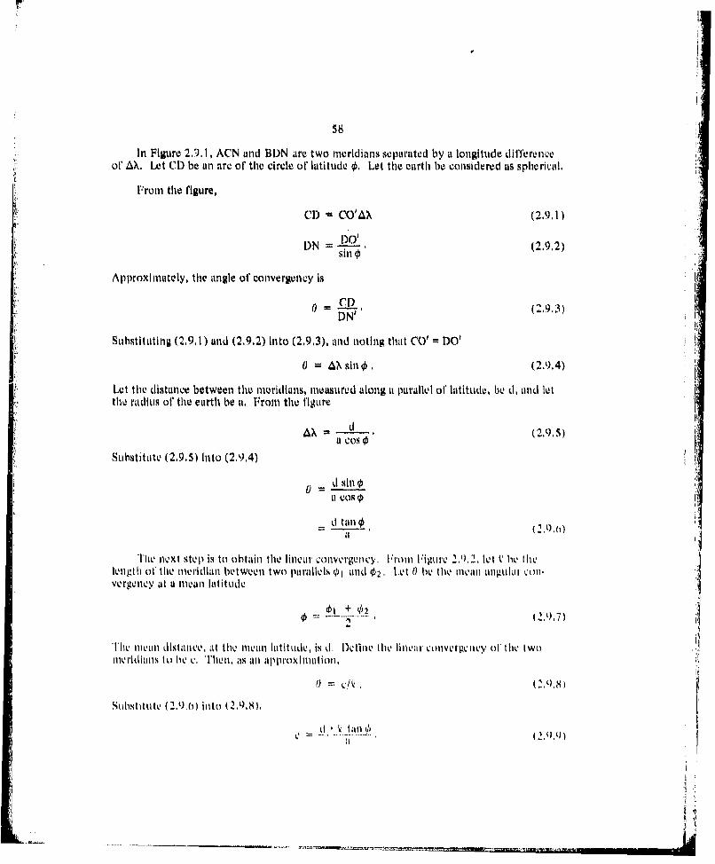
In Figure 2.).,1, ACN and BDN Lire two meridianisseparated by a longitude differenceor AX, Let CD be anl are of the circle or'latitude ~.Lot tile earth be considered us sphiericall.

From thle figure,

D C'A (2.9.2)

Approximately, thle angle of convergency is

CD (2.9.3)

Suhstitilting (2,9,1) and (2.9.2) into (2.9.3). and noting that CO' =DO'

0 = AN Sinll (2.9.4)

Let the distance between thle mneridians, measured along u paLrallel Of'latitutIV, be d, and lotthe radiuis of' the earth be a. From tile tigUre

AN - (2.9.5)a cos o

Substitute (2.9.5) Into (2,9,4)

a Cos

The nevxt ste p is to obtain the Hlnear1 conivergenicy F rom l'igu ic 2.).2., le t V he tilelen gth of the meridian betwenl tWO parallelCS @1 1,1nd 02 .0e 0 be the 1man an1gLar1 Qonl-vergeney at ai mean latfitude

Tlie 11ean1 distanlce, at tile mean latfitUde, is d, Dicliie the it cunVIIV0erOgeiwy ot the twomeiridhis to ho C. 'Thenl, as an1 approximaltionl,

0 CA,(,95

Substituite ( 2.9,0) into (1,9.8).

Lid

59

No.

Figure 291. Gomantry for mgu~ar ooswupnes of Uw mmidhem

60

d

01

Figure 2.9.2, Geometry for linear convergence for the merldians

61

2,10 Rotation of the Coordinate System 1201

A rotation of the coordinate system cun be defined to conveniently obtain oblique,transverse, and equatorial projections from polar projections, This cun be conveniently doneby applying formulas of spherical trigonometry, The spherical trigonomnetry approach isJustified, since In Chapters 4 and 5, It will be shown that anl Intermediate transformation canbe performed for the equal area and conformal projections which transforms from positionsonl the earth to the authalic or conformal sphere, respectively, Once this is done, thle rou-tion formulas for the sphere can be applied directly, Also, the conventional projections ofChapter 6 are based onl a spherical earth for the majority or their practical applications.

Figure 2. 10.1 provides the basic gvomnetry for the rotational transforination. Lot Q betiny arbitrary point with coordinates 0 and W~ onl the earth. Let 1P be the pole a1'the auxiliaryspherical Coordinate system, InI the standard equatoril Coordinate system, 11 has the coordi-nates 01, and Nil Let hi bet the latituide of Q in the auxiliary system, and cy, theQ lonigitudeI in1that same system. A reference mecridianl is Chosen for the origin of' mneasurement ot'cy.

The intention is to derive the projection III the (11, a) systeml and thenl t ranislorml to tilt(,X) system t0'om' the plotting of tile Coordinates.

nhe reations between the angles of interest Can be founld from file sphierical trianglePNQ,

Vrom the law of cosines

Cos (90" - 0) Cos (90, - 011) Cos (90 - 11)

+sill (900 - 010 sinl (900 - h1) Cos (v

Sin 1) sinl 01 sin 111 + Cos 0,Cos 11 Cos (v (.0

F~romt the law of sinles

sin l ( Xf - NO) s i ( k,sin (90 -1 sill 00 c 0)h(.1

silcos 11

Also, Lipplyl ng the four parts fornitili

Cos (900 - CL)5 (v -sinl (40 -~ oi) cot (9f00-

-sinl (' Cot (h - X1

sinl /jil cos (V Vcusol Im tan h Sinlco (X Ll I

cot N il I O /J1 .a . (i P1, Io aclSillA (21V

62

PP

Figure 2,10.1. Osametry for the rotational trmnsformation

63

The inverse relationships atre also of use, From the law of Cosines

cos (9Q0 - h) cos (900 - 0) Cos (90 0 -

+sinl (90 ° - 0) sin (90* - OP) cos (X - NP)

sill h= sin sill OP + cos 0 cos OP cos (X - Xp) . (2.10.4)

From the four parts form a

Cos (90' - p) cos (X - ) sin (90° - Op) cot (900 -

- sil (X - ,p) cot ca

sin O col (X - X co C tln i - sin (X - Xp) cot a

sin (X - Xp) cot a cos 01, tim 0 - sin cos (X - Xp)

si (X - xV)t(2 10,5)

coS 0, tall S -i , Cos (X - Xp)

. ilnal useful Cqtuation Is needed for unilue quadrant dutermination, From a consideratIonat' Figure 2, 10. 1cos C cos h t sin vos h1, - Cos sin 0, coX- XP). (2. 1016)

I laving possession of equations (2,10.4), (2,10.5), and (2,10,6), we can accomplish tinyrotations iveusstiry to form oblique, transve se, aid equtitortil projections I'rom polar andregular pro~itlons. 'lhes will he required In some of the projections ol' ('hapters 4, 5, and a.

, t

Chapter 3

FIGURE OF THE EARTH

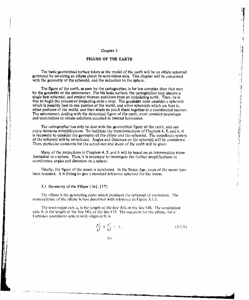
Tile basic geometrical iurtace taken its the model of thle earth will he all oblate spheroidgenterated by revolving an ellipse ubouit its semi-minor axis. This chapter will be concernedwith the geometry of the spheroid, and thle red action to thle sphere.

The f~gure or thle earth, as seen by the cartographer, is for less complex than that seenby thle geodesist or the astronomer. For his basic surfa~ce, the cartographer may assuime itsingle best spheroid, and project thereon positions from an undulating earth. Then, hie is%free to begin thu process of projecting onto it map. The geodesist nmst consider at spheroidwhich is possibly best In one portion of thle world, and other qpherolds which are best inother portions af' thle world, and then strain to patch them together In it coordinated manner.The astronomer, dealing with the dynamical figure oit thle earth, motst consider peur-shiapcand undulations to obtain solutions couchied in tesseral hairmonics,

Thle curtographer has only to deal with thle geometrical figure of' the varth, and canenjoy immenseel simplifications, To facilitate. theQ tra~nsformationlS ofC'hapten- 4,.5. and (), itIs necessary to consider the geometry o1' the elliplse and the spheroid. The coordLina1te systemof thle spheroid will be introduLced. Angles and distances onl the sphberoid will Ne considered,Then, particular constants l'or the atiual sizo and shape of' the earth will hie given,

Many of the projections In Chiapters, 4, 5, and 6 will he based onl an Intermediate trails.formation it.) a sphere. Thus, It Is necessary to Investigate the lute ipi'ctill icoordinates, anglus and distances an at sphere,

FinlliY, tile f1gUro o'l the moon is developed, In thle Spiace Age, imips 01 the moon havebeei n reqired. It Is lltting to give it standard rveereniec sphevroid for thle moon.

3.1 ('iomotry of' the iIlipse 116 lb I 171

The llipse is thle geneorating cu~mv whichl prodluces tile splicroid ol revolution. The'n1onienlehi nre o I thle cli pe is h~est descri bed with ic lere icc. to lgllrc . 1.1

'rhc svini-m-oor axis, at, is thev length ol' the lie A0, or ilie lie 011l. Thv seni-minoraIXIS, 11, Is the length oit thele 11V DO.r the linle CO0, Tlhe cuitltion l the e10 lliplse. I'or a('artesian Coniinat syste il with origin 'at 0, Is

(.'4

65 I

A C

Figure .31. 1. Geometry of the ellipse

66

te degree ol' departu.-t from Cir-cuIlarity is described hy the eccentricity, le, or tileflattening, f'. The eccentric,ty, flattening, sei-major axis, and sciii-minior ax is are relatedits follows:

e2 u2 - b2 (..)L12

02 2f - f 2 (3.1.4)

At this point we shall introduce one of' the two anguilar coordinates which uniquelylocate a position Oil thle spheroid. This first coordinate Is thle latitude, Two types of' latituidewill be noted: thle geode~tic and thle geocentric, The relation between thle two will lie derived,

Thle geocentric latitudO IS thle an1gle between at vector 1'ron the center ol" the ellipse, toat point l1, oil thle ellipse, and thle send-major axis. The geodetic Il tadeLI IS tile an1gle betweena line through the given point, normal to thle ellipse, and thle Nei1major axis. This nor-mat to thle lliseu is thle line def'lIed by a1 survyor's p~lUmb line it' till gravit y Lulomaliesire Ignored,

Now, consider at polar coordinate system with thle origin ait 0. The geocentric latltiude,',is 4COP, and thle mlagnlitude of' the vector is r, The relation between thle Cartesian and

thle polar coordinates Is

x = cs~ (315)S

z = 1) sill' (3.1 -6)

litiations (3. 1. 5) and (3.1.6) can be com1binedL to I'0rm1

T 7tall 0' (3.1.7)

Substitute (3.1,2) Into (3.1.7).

01' greater interest IS the geOdetic latt(de , q). This MngIO, A PQW, d fL11110 111 ldie liationloF, line QV. which Is normal to thle ellipse It point 11,

d \t a it - 3

67

Taking the differential of (3,1.1)

2x__X + LZ-Z = 0a2 b2

dx u2 zS= b (3.1.10)

Substitute (3.1.10) ito (3,1.9).

tai (3.1,11)tas=b2 x

Substitute (3.1.7) into (3.1. 11)

q2 btail~ tail

tatil~ ~ tant U~ btm (3.112)

Substitute (31.2) into (3112).

tan1 ' +v1 L - tlt (3113)

Table 3. 1, 1 gives the relation between geocentric latitude and geodetic latitude for theWGS-72 spheroid, which will be discussed In Section 3.4.

The convention for nmi.auring geodetic latitud t is +0 In the nortlhrn hemi p hre, and€ in the southern hemisphere,

3d

.................................................................................L. ~..d~h~~Jd~

6H

Table 3,11,1 Geocentric and Geodetic Latitude forthe WGS.72 Spheroid (Degree,.

Geodetic Geocentric Geocentric Geodetic

0.00 010000 0100 0100005.00 4.9833 6.00 5,0167

10.00 9.9672 10.00 10.033015.00 14,9820 18.00 16.048220,00 19,9383 20.00 20,081925.00 24.9204 20,00 25,073830,00 29.9188 30.00 30.083435.00 34.9097 35,00 35.090B40.00 39.9053 40.00 40,094845,00 44,9038 45.00 45,090250.00 49.9053 50.00 50,094755,00 64.9096 55.00 55,090480.00 B9.9167 80.00 80.0833G5.00 64,9263 65.00 85.073770,00 69.9381 70.00 70.081B75,00 74.9519 75,00 75,048180.00 79,0671 80,00 M00329835.00 84, 9833 85.00 86.01070OC90.0 M0000 90.00 90.0000

t 69

3.2 Geometry of the Spheroid 1231

The spheroid, which is taken its the model of the earth, is obtained by revolving thleellipse of Figure 3. 1.1 about thle z-a~is. For the Cartesian coordinate system shown IIIFigure 3.,.1, the equation otf the spheroidal surface is

x2 y 2 Z2+ -, +-. 1 31

112 a12 b

The nomnenclature of' thle spheroid can be obtained by studying Figure 3.2. 1 Each of'thle inflnl1ty of positions of the ellip1se as It is rotated about the z-axis defines a meridianalellipse, or meridian, The angle X, measured in the x-y plane, and from the x-axis, Is thelongitude of any and all points on the meldanal ellipse. This Is the second or thle twoangular Coordinates which uniquely deflne a position on the spheroid. As a convention, arotation from +x to +y will be positive, and the reverse rotation, negative,

Consider the point 1P in figure 3,211 to be defined by 0 and X. Suppose now that X isfallowed to vary, while 0 Is held constant, The locus on the spheroiu traced out by P Is acircle of' parallel of' radiuls It. The circle of parallel for- a latitude of zero Is the equator.

It remains to derive the equations lor several radii of Importance inI futuie develop-mnents. These are the two principle radii of ell rat tre, and the radius of' a parallel circle, tillas a function otf latitude

C'onsider the nivridiunoil ellipse ait any a ihit vary X,. l~rom (3,2. 1

zi 2 2 1(3.2.2)

whiere Ito .%/_XT;y7 is lthe nitdhis of toa parallel eilr-Cie.

Suibstituite (3.1,2) into (3.12),

V.

t1 2 (I --.V

C21 -c) + /2 L1 -2 . 3. 2.3)

lake the dilfeTIV11tial 010.1.3) t10 o1htil tile sloiwe of' the talnt tiat P1.

2Roo di~~ IJ 0 + zL? (

Rol 3. .4

iI,

70

I.

Figure 3.,.1. Geometry of the spheroid

71

The slope of the normal at P is again

- tandz Ro(l - e 2 )

z = Ro(I -" e2) tan , (3.2.5)

From Figure 3,2,1

S UPO - C2) si 0 (3.2.6)

Substitute (3.2.5) into (3.2.3)

R2 (I-C) + R2(1 0-c2)2 tan 2 = a2 (1 -e 2 )

R2 + R2(0 -c 2 ) tan 2 0 a2

(cos 2 0 + sltn2 ) R2 - e2 R 0 si= 2 a2

12(I - e'2 sn 2 0) = tU2 COS2

a CosR) - (3.2.7)

Also, from Figure 3.2. I

RHI = Q" cost, (3.2,8)

I~qtLatitlg (3.2.7) and (3,2,.8)

cos 0 d cos

(I is th IIC riIdius 0 c Oiivatuiof ik. Splhtroid il IL jl IWr'llei lCIctula '1 the 1ueridi11alplatit, ald will h devoted as Ip.

72

URP u (3.2.9)

The radius of curvature of the meridlanal ellipse follows from the formula for a planecurve (2.1.35),

RM -(d~ 3.1,10)d2 z

d R'

From (3,2.4)

d2 z 1 e2) + R 10dR2 7z LIR

Substltutilng (3.2,4) into (3,2,10) F 1d2 I e- 2) _ - -

dR 2 z T Zo

A ( I /d-- 7 \ - ' (3.2,12)

Sitcc thIi slope of tI w n rniaI is thn 0, that of tIie tangent --cvt 0.

LI = cot , 3,2,13)

SubstitUti1g (3.2.13) in to (3.2, 12)

_z I + cot 2 -- e

d Rn z

s i 2 q. 1 4 )

!:1

~.~.,...

73

From (3.2.6) and (3.2,9)

Substitute (3,2.13), (3.2.14), and (3.,.15) ino(3.2,.10).(3/2( sn2~ / ~ -e2)=Sin1

CS2~ + Sin 2~

JI1 2 ~ /t I( - e2) Sill

10 -0),in

FIutions (3.2.7), (3.2.9), ujnd (3.2.16) give the radius of the circle or parallel, therudius of curvatuire normal to the meridian, and the radius of' curvature in the moridianalplane', respectively. The radii ol' curvature arN talbulatedI in TAWl 13.2.1 ats fun ctions of latitudefor the W(GS-72 spheroid (Section 3.5),

Before turning to ditancos on the sphecrOid, it will be usef'ul to relatte the ('artesiancoordinates tor the siwroidl to the ipolar coortlimates-,

x Rp cos~ 0 -os N

y -Rp O cslsirA 03. 217)

1 (I~RI Sii.2 ll

74

Table 3.2.1. Radii so a Function of Latitude.

Radii of CurvatureGeodeticLaotitude *

0,00 6378166. 6335477.5,00 6378327. 8335980,

10.00 6378809. 6337385,

15.00 8379595. 6339740.

20.00 6380663, 6342924.

25.00 6381981. 6346854.

30.00 5383508, 6351411.

35.00 6355199. 6356480.

40.00 6387002. 6361847. V45,00 8388864, 6387412,

50.00 8399727, 6372985.55.00 6392536, 6378396,

60. U0 6394234. 6383481.

65.00 63955770, 3388082.70,00 6397096. 6392058.

80,00 6398967. 6397667.

75.00 639817, 6395287.

85.00 (3300453. 6399126.

90.00 0399617. 6309617.

*Degroev**Motors

rI

75

The first fundamental form of the spheroid (Section 2.3) becomes

(ds)2 = R2 ((1)' + R2 cos2 ¢(d,) 2 (3.2,18)p

Equation (3.2, 18) will be useful in the transformations from the spheroid to the sphere in

Chapters 4 and 5, and in tile discussion of distortions in Chapter 7.

3.3 Distances and Angles on the Spheroid IS I

Three types of distances measured on the spheroid will be considered, Thes are dis-tances along a circle of parallel, along tile nerldiantal ellipse, and between two ordinarypoints,

We can deal with the distance along a circle of parallel very easily. From (3.2.7)

d = aAX cos 0d e~(3-3.1)

where AN is the angular separation of two points on tile circle of parallel, in radiamts. Table3.3,1 Oves the, distance for an angular separation 01' I' tm a function of latitude for theWGS-72 ellipsoid.

Distance along the meridlanal ellipse requires an integration of (3.2,16), To l'atllititethis, (3.2.16) ls,expanded by the binomial theorem.

a(I -e0) 1 esgi 2 r + e4 shn4 + ObS116 + (3,12)16

Equation (3,3,2) is it rapidly converging series, as we shall see when we display the values ofe hi Section 3.4.

Tihe distance betweeni positions at latitude 01 and 02 on the sulle niridialai ellipse are

d I R.. (i0, (3.3.3)

Substitute (3.3.2) int6 (3.3.3) and Integrate

d- al-' 1 4 e- e2in , s Lit;4 14 + ef'sil6 +fI

76

Toble 3.3.1. Distances Alongthe Circle of Parallol for a

Separation of 1',

GeodeticLatitude Dlitance

0,00 185,3325,00 1848,31

10,00 1827,32V

15.00 1792.51520.00 1744.1242E,00 1682,50730.00 1608.1103500 1521,47440.00 1423,23545.00 1314.11850.00 1194,93355,00 1066,6726n.O0 930.00265.00 "786,26070.00 636,44375.00 481.70180.00 323.22585,00 162,24190.00 -,001

*Degroes**Meters

77

2i 2( 4c2 S in 2 )

+ 4 + C ( + /J "'

-- (I-,C 2) ¢ (i + e2 + + '_~~ 353 l ( ', ,,€2

{( 45e4~~~~si 45 ( 2 : ,)

+( hI Cos + 175 +

NI1r. 6 ii32

j ~ 6.2 4 768 ,.>

02 .- 15, 04 + 17 C6+ , , i~

32 334 3

L !6 C L) s(0 + 112

88 32 32 384

78

d = a {( -1 e4 5 e6 -

4 04 256 "

3 2 + a 4 6+ ill 20 1

+32e 3 84

+(. 4 6 )l 40 t

'"253072 + .i4

35" -- - (3 -4 Cos 20+Cos 40) , 334)1Further expand the last term ini (3.3.4)

-9 e6 (51 (3 -4 cos 20 + Cos40)96 16

- - 5 C6 (1i sin ---- L sill 20 + -j- sil (nlo (3.3.5)

96 16 833

Substitute (3.3,5) into (3.3.4).

d I V( 4 et.~

V2 I + .4 + 0- -, .S' + +"ilF- 2 ,-384 + 6( 32))+,,,

+ 4 (4-, - +.I's oL' q., s1im 40L 256 ~ ,3072 90 8),

9o 32 +

4 i-(_3 2( + 3 - 4 + 1 6 + ilH

8 T2 + 1024 +..

+ ,(1-5 4 + 0."--" e6 + sin ,40 ,- 30-.5 e6 sin , 60 +. (3-3.6)'256 1024 ''' -3072 L101 6 ..t1quation (3.3.6) has been evaluated in Table 3.3,2 for ' intervals of arc along the

meridiumil allipse us a function ot' latitude for the WGS-72 spheroid,

Tlhe distance along a spheroid between two arbitrury points P1 (01, Xl) and P(2, X2) IIIs obtained from consideration ol'the first fundamental form for a spheroid (3.2,18).

f (a)'] ~ (3.3.7)q

To obtain the hortest line on the spheroid Colecting I> mnd P2, that Is, the geodesic curve,apply the 1uler-Lagrange relations to (3.3.7), where

L(O, X, 76 -)R= + Rt2 COS2 (')d [)L\ Thd~ (oL) (IL

0aL c (3.3,8)

whenr c Is a constant.

Substitute (3,)3.9 to (3,M37).

It re illnl H ti evaluate c In (3.3,)), Int'grale (3., ').

+ k. (3,-,10)

Substitutw (3. 2.1) into 13.3. 10).

Table 3.3.2. Distance Alongthe Meridioal Ellipse for'

a Separation of 1'.

GeoodeticLatitude Distance

0.00 1842.9145.00 1843,055

10.00 1843.47215100 1844,16420.00 845.08125.00 1846.22430.00 1847,54938.00 1849.01840.00 1850.58545.00 1852.20450.00 1863.82565.00 1865.39960,00 1858.878t6.00 1858.21670,00 1859.37375.00 1860.31280.00 1861,00586.00 1861,42930.00 1861,572

Degree -"

81l

- f(i - Csn2) d +

= d + k

e2 o,, 2 dO

1/ 2 C 2

+ -J02 4J!U 2 cos2, 2 /

an- + _ + k (3.3.11)

E'vuluatc (3,3. 1) Lit P, lilld P2, and subtract to climinu t k.

X,= C C t1,10 +- VAL.0) + k i

X2 C tall + i 41 2 ]+4k

[(i--(41 -,'P ]

X2 - -

,- 4= {UC2n,3 .1,2 12)t2

.122X2sit t X 31 , ) C 3 2 1 ' n (11111 , 111111nlo ( 02 -00

s ~ ~ Ml 2h U11 0 1.' S~l€ ) +l (.42¢

02/

(3..16 an (33 ) 2 (33,h

S11120

X 1 2 - 2

00i

Han. _ tal(2 O!a

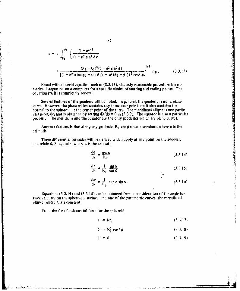
82

f02~IJ ( -02)22 |- shin2 0) 3 z

+ ,2 - 1)2() - e2 sin 2 ) 11/2+ do 3.3.13)(( e2 )(tanl 2 -tl'10i) - e2(02 -01 eo82 0J 1 3*.3

Faced with a horrid equation such as (3.3.13), the only reasonable procedure is a nu.merical lnte.ratlon on a computer for a specilic choice of starting and ending points. Theequation itself is completely general,

Several features of the geodesic will be noted, In general, the geodesic is not a planecurve, However, the plane which contains any three near points on it also contains thenormal to the spheroid at the center point of the three, The meridianal ellipSC Is one partic-ular geodesic, and Is obtained by setting d/do = 0 in (3.3.7), Tht equator Is also a partIculargeodesic, The meridians and the equator are the only geodesics which are plane curves,

Another feature, Is that along any geodesic, RI cos m sin a Is constant, where a is theazimuth1

Three differential formulas will be derived which apply at tny point on the geodesic,mnd relate , a, and s, where a is the azimuth.

d._ = s (3,3,14)

ds Rill

LIN I Slds RI, Cos (3.)

(la I- tafl Silla( 3.1(Ii,

Equatlons (3.3.14) mnd (33.15) can be obtained from t consideration of the angle he-tweon a curve on the spheroidal surr£1ce, und one of the parametric curves, the niridlhnalellipse, where X Is l constant

F rom the flrst fundamental form for the spheroid,

I = (33,17)

G R C, ;5 iIS)

F 0)~,.t

83

.14

Figure 3.3.1. The aimuth of a curve'

84

Since X1 c

Al1 0 (3.3,20)and

ds I %/T do (3.3,21)

E Edo do + Gd>A AlCos~ Q = - (3.3,22)

Substitute (3.3.20) and (3.3,21) Into (3.3.22).

Edo dotCosa=...*dd 1

/E- LO , 3.3.23)ds

SUbstitute (3.3.17) into (3.3.23).

This has Justifled (3,3.14).

v~(do i Al - do At 3,,4

sill a (3.3.24)~/~da dX

Sill

Substitute (3.3. 18) into (3.3.25).

silla =R 1, Cos X .Lis

This is (3.3.15).

F~rom (3.3.14) a~nd (3.3.13), the azimuth at 1) at the initiation of the geodesic can lie

C'alculated.

- ..........

do5

COS ul R

a(Rn1 1 {0 -e2 S 1

+ [( (X ~i 2 (1-C 2 in2 i) ~ /2 (3.3.26)[I- e2 ) (tail0 - tanoi) - e(0 -001 2~

The rhunibline (or loxodromne) Is a curve onl the spheroid which meetq each consecutivemeridian at the some azimuth, From Figure 3.3.2,

taliCe = cosn do O

A=tane a cos do . (3.3.27)

Substitute (3,2.9) and (3.2,16) Into (3.3.17),

a - 02 ) COS

(I- C2 Sin12 0)./ 2

I - c2)si1 I(I /C I -

tailna jtail z. + 0 .1l (3328

The kernal otf (3.3.19) will bo Seen again when we treat the von formal pirojections of 'Chap.ter 5. The rhumbline, used In conjunction with the Mercator projection (Chapter 5) and thegreat circle onl the gnomoic projetetion (C'hapter 6i) Lire longstanding aiids to marine andaerial navigation.

96I

Figm.3.3.2. Dlffoential elemant dfininga rhumbll n es *MPidSO

87

3.4 Geodetic Spheroids 151, 171, 1181, 1211

Beginning in the curly 1 800's, a serious attempt was made to find the correct dimen-sions of the earth. Geodesists and surveyors undertook to find the best representation.

The physical shape or the earth is too Irregular to be used in any mathematical study,Thus, it was necessary to define a fictitious surface which approximates the total shape ofthe earth. The surfaces of revolution of this section are the geodesists answer to the problem.They are the most convenient surfaces which best fit the true figure of the earth.

The geodesist's first approximation to the shape of the earth Is the equipotential surfaceat mean sea level called the geoid. The geold is smooth and continuous, and extends underthe continents at tle continued mean sea level. By definition, the perpendicular at anypoint of the geold is in the direction o1' the gravity vector. This surface, however, is notsymmetrical about the axis of revolution, since the distribution of mutter within the earthis not uniform. The geold Is the intermediate projection surface between the irregular earth,and the mathematically manageable surface of revolution.

The estimates ol the values of the semi-major axis and the flattening have changed overthe last 145 years, Progress has meant better instruments, better methods of their use, andbetter methods of choosing the best fit between the genid and the spheroid. The instru-ments, their use, and the statistical methods of redutcing and fitting the data tire beyond thescope of this report. Nevertheless, we must be aware .tf their existence, and their contribu-tion to mapping,

Table 3,4,1 gives the names and dates of important rference spheroids, as well Lis theequatorial semi-major axis, a, and the flattening, f, of the ellipse, Historically, the first ofthese spheroids, the Everest through the Clarke 1880, weru intended to fit local areas tit theworld. Beginning with the I layford spheroid, an attempt was made to obtain an inter-nationally acceptable representation of the entire world,

Progress has continued In refining the values of the semi-major axis and the flattening.ThLe best representations available today are the World Gravity System of' 1972 (WGS-72)and tile In ternalanul Union of Geodesy and Geophysics of' 1975 (1.U.(;.G,) values, TheWGS-72 'alues will be used in this report.

Unfortunately interest in generating tables such as Table 3.2.1, 3,3.1, 3.3.2, and 4.1,1,and the lotting tables of the projections has flagged since those similar tables incorporatingtie Clar!-e 1880 and Ilyford spheroids were published 1251 . Thus, the tables icluded inthiki repu,'t, using the WGS-72 spheroid, are the most recent representations of cartographictItMa available.

Consider n1ow the WGS-72 spheroid, Using (3.1.4), the eccentricity of the mierldihnalellipse is 0,081819. From (3.1.2)

1)2 = a2(I- e2) (3.4.1)

Using W(GS-72 plrameters, b = 6356750 metrs, Thus, the difTerence in length betwen taeequatorial and polar iixes is 21385 meters.

Table 3.4.1. Reference Spheroid.

Reference aSpheroid Date (meters) f

EVE REST 1830 6377304 1/300.8BESSEL 1841 6377397 1/299.2

AIY1858 6377663 1/299.33CLARKE 1858 6378294 1/294.3CLARKE 1866 8378206 1/295CLAR1KE 1880 6378249 1/293.5HAYFORD 1910 6379388 1/292.0KRASOVSKY 1938 6378245 1/298.3HOUGH 1956 6378270 1/297.0FISCHER 1960 6378168 1/298.3KAULA 1961 6378165 1/292.31.,U.G. G. 1967 6378160 1/298.25FISCHER 1968 6378150 1/292,3WGS72 1972 6378135 1/298.26I,1U. G.G. 1975 6378140 1/298.257

The eccentricity figures in the series expansions developod In this chapter. It has beendemonstrated by Table 3.4.2. In the table are Ibowvrs of' c for the WGS-72 sphieroid, Notethat: considering the seven significant figures for a, It Is not necessury to curry any expansionbeyond 06 ,

Table 3.4,2. Powers of a for the WOB.72 Spheroid.

an noi

1 0.01819 4 0.000044812 0.008694315 6 0,0000036673 0.00054772 6 0.000000300

90

3.5 Reduction of the Formulas to the Sphere 1221

The most simplilied iiodol or the earth Is the sphere. In the spherical case, the gen-crating curve for the surface Is the Arcle, which is an ellipse ot zero eccentricity.. The s .nd-major axis and semi-minor axis are the same. This offers immediate simplitications ''. Ir theproblems of distance, and angular measure. The spheroidal formulas, in gets, , 1, can be re.duced to the spherical by substitution of e = 0. However, the formulas for distance betweenarbitrary points, and a.imuth can best he approached by spherical trigonometry,

The equation rot the sphere In Cartesian coordinates isx2 y2 z2 f- - - i, ( ) Ia.2 , al2 al2 i

Figure 3.5, 1 gives the goometly of the sphri'al earth. Note thut the normal to the sphereat a pulint, P, coincides with the geocentric radius vector,

For the sphere, there Is only one type of latitude, shne geocentric and geodetic latitudescoinlide., Longitude is measured in the same wly it was for the sphoroldal t'ase, 'The signC0If11ns for lttude and longitude in the spheroldal case alo holds ror the spherical case.,

The radius of' a circle of parallel becomes, by substituting e = 0 Into (3.2.7)

R a cosr, (3.5.2)

By the same substitution, the radii of ca rvuture (3.2.0) an1d (3,2 16) are found to be

a11, = R11 . (3.5,3)

The relation bet Ween ( 'artesian and polar coordinates lollow fronm (3.2. 17).

X a- Cos COS S)

y acosi I I (3.5.4

z a sin 9

The III-it fun1damental form is, from (3.2. I )

(s 4 a2(d) + 12 coNI(dl) 2 , (3,5,5)

Distance along the circle of parallel Is, from (3,31)

d AN Cosp 356

From (3,3.6), distance a long (he meridhm circle is simply

11:: A0 ,( ,57

91

Merldlan

Figure B,. I GeOmetrY Of the sphere

I,

92

On tht sphere, tile shortest curve connecting two arbitrary points is in arc of the greatcircle. The great circle (also called the orthodrome) corresponds to the geodesic curve onthe spheroid, but with many simplifications. The great circle is a planar curve which con-tains the two Larbitrary points, and the center of the sphere. The distance on the surface ofthe sphere, can be obtained from consideration of Figure 3.5,2.

The equations of spherical trigonometry will be used to derive the distance, d, Con-sider the law of cosines.

cos 0 = cos (90'- 1) cos (90-@ 2)

+sin (900 - 01) sin (90 - 2) cos AN

sin rl S'1102

+ e8 1COS 0o2 COS ;, (A..%

Taking the arc-cosine of (3.5s8)

d =a cos t1 sin1 sln112 + C05S0 cos82 cosA,J (3,5,9)

The aZih1uth, Q, of point Pt from P2 is also obtained from the Spherical triangle NPIP2. Taking the arc-cosine oh' (3,5,9) again, the angle 0 Is now available, Then, the law ofsines is applied.

Hill a sIll AN

sill (90 ° - 2) =

Sia O= "1 (3.5,10)

Also,

cosav cos 0 cos (00 - 0 ) + sin 0 sin (90' - 0l) cos (90 *-02)

cos a = Cos0 sinl 0 t + sin 0 Co04)0 sill2 (3.5,11)

From (3.5, 10) and (3.5.11), the quadrant of tile azimuth can be seen. As was men-tionmd in Chapter 1, azinmtth is le.asured from the North, positive to the Fast, aid negativeto the West,

The rhumbline or loxodrome is olitained from (3 3 , 28) by substituting in (3.5.3)

rT @2"/i

tuna ~ . +ii ta ( - Inl tanl + (352

lIquiatio (3.5,1 2) canl be investigated, It' 1 - t hen o.' nT 0, E.\ 40, This is an azimul11thi ~~alon~g at rallel circle. Ir ) = X, tua'. 0 , a' 0=, yielding a mer'lidian.

93

N

PII

Piper 3.5.2. Dhewso bstws abitrary points on the mphe

941

The distance along the rhunibline Is found from Figure 3.5.3.

5=1 ds P csad

-S~ (3.013 jAs was mentioned before, the great circle and loxodrome will be mentioned again In

conjunction with the Mercator and gnomonic projectionis.NI

Figure 3.5.3. Differential elemnent defining a thumbline one asphere

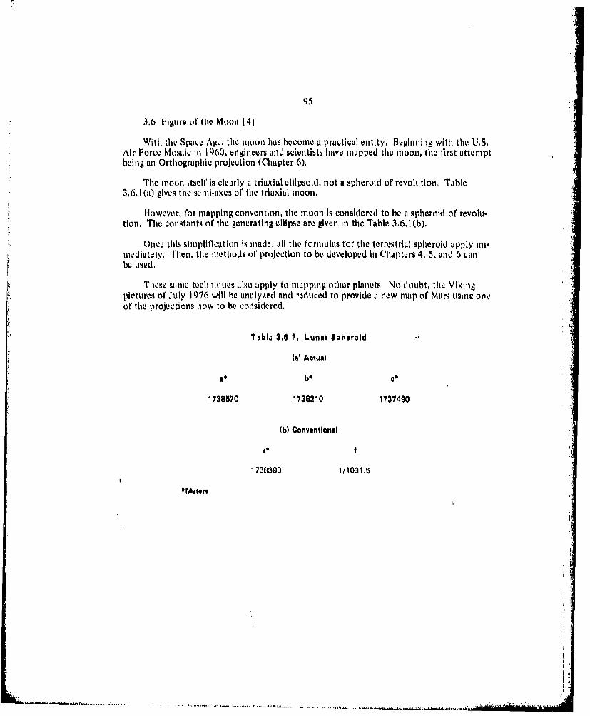
95

3,6 Figure of the Mooni 141

With the Space Age, the moon has becomie a practical entity. Beginning with the U.S.Air Force Mosaic in 1960, engineers and scientists have mapped the moon, the first attemptbeing an Orthographic projection (Chapter 6).

The moon Itself' is clearly a triuxial ellipsoid, not u spheroid of revolultion, Table3,6. 1(it) gives the se mi-axes of the triaxial moon.

However, for mapping convention, the moon Is considered to be a spheroid of revolu-tion. The constants of the generating ellipse are given in the Table 3.6,1 (b).

Once this simplification is made, all the formuilas for the terrestrial spheroid apply im-mediately. Then, the methods of' projection to be developed in Chapters 4, 5, and 6 canl

L be used,

These Samto techniques also apply to mapping other planets. No doubt, the Vikingpictures of July 1976 will be analyzed and reduced to provide a new map of Mars usiniz ortoof the projections now to be considered.

Tablo 3,6,1, Lunar Spheroid

Wa Actual

1738570 1738210 1737490

Wb Conventional

a f

1738390 1/1031.5

*MeIters

. . . . . . ..

Chapter 4

EQUAL AREA PROJECTIONS

The requirement which underlies all the projections In this chapter is stated as follows:Every section of the resulting map must bear uacbnstant ratio to the area of the earth repre-sented by it, This requirement will be stated in mathematical terms. Thus, all of the projec-tions of this chapter are futnded on some algorithm which maintains the equivalency of area,

As in any endeavor, there is a hard way and an easy way to work. The cartographersof days past attempted to transform from the spheroid directly to the developable surface.The easier, and more modern approach, is to transform from the spheroid to the equivalentarea sphere, and then transform from the sphere to the developable surface. This results inequations which are far less cumbersome. This chapter follows the modern approach,

First, a transformation is derived which defines an authalic sphere. This authalic spherehas the same total arca as the spheroid. The longitude of points is undisturbed by the trans-formation, I However, the transformation requires the definition of an authalic latitude onthe sphere, which corresponds to the geodetic latitude on the spheroid. Also, the radius ofthe authalic sphere must be determined,

Second, positions transformed to the authalic sphere are then transformed onto selecteddevelopable surfaces to form a map.

The projections to be discussed are the Azimuthal, Conical, and Cylindrical Equal Area,"the Bonne, the Werner, and a selection of world maps: the Sinusoidal, Mollweide, Parabolic,Euniorphic, Eckart, and Hanmner-Aitoff, In addition, a simple means to minimize extremedistortion is advanced in the Interrupted projections.

A quantitative over-view of the theory of distortions is put off until Chapter 7, wherethis t heory will he applied to the most useful of the projkctions en masse. Plotting tablesfor selected projections are given, The computer program which generated the tables isAppendix A. I.

4.1 Authalk' La(lude 121, 181, 1201

Autithalic latituode is defined by the equal area projection of the spheroid onto a sphere.

Front the fundamental transformation matrix of' Chapter 2, and the condition ofequivalency of area:

g9

aO a@A 12

eg - f2 = I(41,1)F G aXA XA

In (4. 1. 1), OA and XA are the authalic latitude and longitude, respectively, on tile authalicsphere, and 0 and X are the geodetic latitude and longitude, respectively, on the spheroid.RA is the radius of the nuthalic sphere.

Both the systems are orthogonal, so

f= F 0. (4.1,2)

On the spheroid from (2,315):

d = R21 dO2 + R2 cos2 dX2

(4.1.3)g =R2 Cos

On the auth-Mic sphere i'rom (2.3,14):

ds2 , R d2 + R2 CO2 A dX2 A

= , (4OA ,

Substitute (4.,1.2), (4.1.3), and (4.1.4) Into (4,1. 1)

50A DOA2

R2 112 eo%2 0 R4 0 2 A(..A CO2 O i)A aXA

3 x

98

The longitude is invariant under the transformation: X =XA. Thus,

(4.1.6)

a?'A 0(4.1.7)

The authalic latitude is Independent Of XA.

04,,8

Substitute (4,1.6), (4,1.7), and (4.1.8) Into (4.1.5)

-0R2 R2 Co62~ R4 C0O5 A

0 1

RR cos2. R2 CoSA 4.A9

Equation (4.1,9) can now be converted into an ordinary differential equation,

Rin RP cos 0dO RA COSOA (1A .(..0

Apply the values or Rrn and Rp derived in Chapter 2.

110 e2)

(I -(ic 2 sin2 0) 1/122.6

Substitute (2.2,16) and (2.2. 17) Into (4. 1. 10).

02 (1 -LC2 )

I~ - 2S11 )

99

Integrate (4. 111)I

A3 f C5AIA=RiPA

COS 0a2 (I - e2 ) - (1. (..c2 ( 2SO02) 2

The easiest way to attack (4.1.12) Is by means of' a binomnial expansion:

R2 si OA a2 (I -es f2 COS(I + 2e2 sin2 0 + We s11n4 0 + 4c6 Sin16 + . .

-1 a(1 - e2 ) Sill + .1e2 Sin3 + 04 esinS 0 + 4,e6 sill? +*,L

(4.1.13)

in order to determine RA we Introduce thle condition that OA = ffI2 Wh11n 7r/2,1

R2~ 412(1 02)(1 + . C + 1 4 + i 6 + ,,(4.1,14)I

Equation (4.1.14) gives the radis Of thle authuie sphere with Lil area equivalent to that of'thi spheroid.

Substitute (4.1314) Into (4.1,13) to obtain thle relation between authalie latitude andgeodetic latitude,

I+ V2 sinl2 +4 C4 Si1 4 ~ + C6 0160jffI +81i1 A =sin~ [ t~ e +746 +..j (1

As was seen in Chapter 3, the eccentricity, v, Is a small numbher I'm Lill of the aceptedspheroids. Thus, (4,1.1 5) Contains rapidly converging series. The relation between authalicand geodetic latitudeIS IN tillalt(d in Table 4.1A1 f'or the WCGS-72 Retetence Ellipsoid, Inlincrements of' 5.

Now that the transformation t'roni the spheroid to the sphere Is comipleted, t he truns-formations 1'rom the sphecie to the developable surlfices will lie derived. In these derivations,thle subscript A onl the latitude, longitude', and radius of the authalc sphere will be dropped,and 0 , X, and R will be the latitude, longitude, and radius, repl ively, of the ant halicSphere,

100

Table 4.1.1. Authali aendGeodetic Latitudes.

Geodetic AuthaioLatitude Latitude(Degrees) (Degres)

0.00000 0.000005600000 4e.97770

15600000 l4.9337720.00000 19690125.00000 24o9015330.00000 29.88686339.00000 34.879091A40.00000 39.8732045.00000 44..87114e60900000 49.87298

33.00000 4.8786760.00000 39.6860265.00000 64s9007770.00000 69. 9165175.00000 74.0347780.00000 79.9550069.00000 84*97bb790.00000 89.99874

Radius of the authaia sphere6,371,037 meters

4.2 Conical Projections 121,. 1201 , 1221C

Two conical equal area projections will be consideredl. InI the first, a cone' Is tanlgeIlt tothe authialic sphere at at single parallel of* latitude. In the second, u cone is secant to it sphere,cutting it Lit two parallels of' latitude, InI both casea, thle axis of the cone coineideq with anextension of' the polar axis of'the sphere, As will be seeni InI the f'ollowing paragraphs, theparallels lit the points oif tangen8cy 0o' secuncy will be the only true length lines onl thle map.

Two methiods 01' approach will be given for ecULh of thle projections,

Thle t~rst is thle ditfferential geomectry approach. The line element onl the authaillesphere iW

dIS2 R2 d02 + R 2 CL)52 dX2

e = R 1g= H 2 Cos,

F~or the polar coordi nate system InIa it laile:

d.42 dp2 + p2 dO02

(4.2.3)

T'he origin o1' 1te projection hlas Coordinai~tes (011i. X~~a), XI be ing sonc longitude onl thlePairallel of' tanga cy, C'oordinate X~ defines the central meridianl oi the ma11 p.

Impose the Conditions that

p p p(0) (4.2.4)

0 + C.(4.2.5)

Tihe constant 1, is z.ero, if' a tu rther condition is that N 0, wheni 0 0.

102

The condition of equivalency of ureai Is:

E F aO 8N~- r2 (4.2.6)

F G aO DO

From (4.2.4)

=0. (4.2.7)

lVroni (4,2.5)

0g4.,o

80

C (4.2 Q)

Substitutiw (4.2.1 ). (4,1.2), (4.2.3), (4.2.7). (4.2.8). und (4.2,9) Into (4.216).

- 0

R4 COS2 0 = I2o c1

10 Co 0 = PC (4.,10)

Tho' minuiasgn Is Chosen1 ice an Increase In 0 Corresnd~)Is to at tkcrease' In p.

Conve'rt (4.2. 10) inito mn ordinary diIfore ntlial equation, and itcgrate'.

onl (lie boundary Conditions Imnposed,

------ --- --

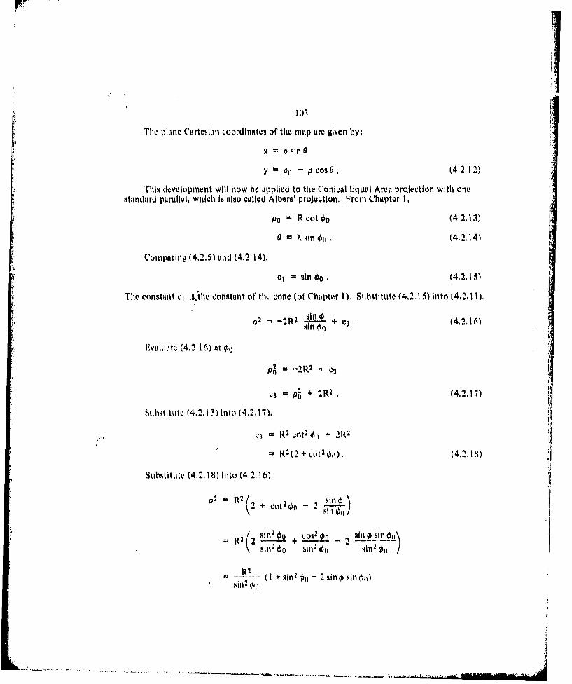
103

The plane Cartesian coordinates of the map are given by:

x = p sill 0

y - P - p Cos 0.(21)

This development will now be applied to the C'onicai Equal Area projuction with oneStandard purallul, which is also culled Albers' projectiun, From Chapter 1,

Po m R coto (42.0

0 - X sillu (4.l4

Comparing (4,2.5) and (4.2114),

C= sinl 00 (4.15)

The constant el isAthe constant of thL cone (of Chapter I). Suibstituite (4.2,1 5) Into (4.2.11)

P2 - -2R 2 '!A + C3 (4.2. 16)sill 0(

LUluLut0 (4.2.16) at 00. -R

3= P+ 1.R2 .(4.117)

StubstItUtO (4.2.13.) Into (4,117).

ei R2 c;ot 2 0(1 + 24) I-R 2 (2 + C(t 2 01), 421)

Suibititute (4.2.18) i nto (4.2.16).

p2 1R2 (+ct~ ~

= 2 22i~2

si2 2

104

% ,IO - 2 (silo2.19)

The CLrtesian plotting equations have been derived. From (4.2.12), (4.2.13), and

(4.2. 14), and Includlng (4,2,19)

, Slp sill (N sill 0)1

y St R vot O - p cos (N, sin )l (4,2.20)

where S is the scalc factor.

Equations (4,2, 19) and (4.2,20) atre the basis of the plotting Table 4,2,1, for 0a - 450and NI - 00, No noc'rized grid is poslIblv: vach map is the choice of the user, The gridthMt result'd for this arbitrary ClioC 1, I- IgUre 4.2, 1.

Two standard pailrllels may also be selected for u secant culi. This projection Is alsocalled the Albers projection, The radii on the nip f'or the standard parallels IN:

PlC Roso1 (4.2,21)

p2 :l R Cos 0, (4.2,22)

Fronm (4,2.5)

X~~ 11cos01 XR0000 = V1 N = Pl P2 (4.2.23)

Substituting (4.2 21) and (4, 2) into (4.2, I1) yi ids

R2 .osI _ l Ip+= 2 "2 I~ + c.

R, CoN2 01 + ZR2 vj siltol - CCl = u (4.2.24)

R2 'os2 02 Rh~2sill 0,2 +1:

R2 co,2 2 + 2R2C1 sill qJ2 - c32 = 0 (4.. 1 )

105ITable 4.2,1. Conlal Equal Area Projection,

One Standard Parallel.

Equal Area Conloal One Standard Parallel

Latltude Longitude* X##

00000 0 O00oo 0con **b69

osponc 15 1 0)a 2,033 - E48O00000 34 399? "3.9210 00 4,C n , 0 0. So82.5 -1 009

0.000 P0.00'o 7s493 -1,?76

0 , C 0 ,0D 1 C , 2" a.2650000009 aO0 0 0 9,09q 1, o73

1! 600011 o, a F n, 00 p"sco 3, 22?t.0O000 t ,OOunn t,761 -5.063

1s,0000 MOM0 3, 476 -20576i,'0000 45,00 o .0 64 -1, 784

5o0000 0,aOf) o , 480 -. 712iso000 19, a 10 7,670 ,602

5.,000 90,a000 8.607 , 13

3060000 0.0000 O. 090 -1a b54

30,0000 1 vu0 t'.7q 11.51730,.nf 00 0.0 000 2s 906 1,- 10930.0000 4t.,OM0 4a P35 . 47?

30,0000 fO~ an 000 5, 4iq 4.1

soto000 0 0 P 0 ? , 19?. 2 12a',50 00 n 0 n, il) 0, 001 coo

05 o000 15,0000 to.1714 109.590090 30,n .0 2 3 0q .432

.5o0000 A)0a d nO a .. 03 1 670

4 ta0 0 00 71j a 0 10 s 96 a '.4134s,0a0o 90. 00]0 5,715 3. 46

60.00 0.000o 0.000 1,646o00O 00 15,ThaJf n ,87%. 1,727

60 aO Ot 30,0010 1. 0:12 1.966

60.so000 1000 2.1.995 "604UOCO 6,In0 00 3a 19 1 2o e896000000 5000 31.781 3, ? s3260 0000 a 0 . a , 240 4, 277

00 = 45C 0 Dgree0 = O 'Meters

---------------------------------------(~j

1 106

r

!4

.1

107

Iquations (4,2,24) and (4.2.2S) can be solved simultanvouily for cl,

j2 Cos 2 0, - R2 eos202 + 21,2cj sin l$ - 2R2e, sine2 - 0

Cosdol - C042 $ 2CI (s2112 -s1n0)

C2( n$2 - in $i)

2(sin 2 -sin0tI

- - s. ( .2in + si1 ,4.22 6

Submtituting (4,2,26) Into (4,,23)

o 0 - (sill $ +Sin l2) 4,227)

Substitute (.4,2,6) into (4.2,11)

P2 4R10 min_ _ (4..2.8)

4R2lo +SIII +

Ivaiutut (4.2,28) at 01

4R2 in$,

4i0 $1 + -in , $

L3p ~i1i + 17l 2 422~

Substitulh (4.2.24) Into (4." 2 )

p(2 p + 4 R 2 (4,2.301

siT@l + 8in 2

wlicl', Irom (4.2,2) mid (4.2.20),

-R cos4,

:i+4

.... ...

A similar deqvopnient will givir,

2 pi + 4R 2 sn + - ifl (4.2.32)

2 R Co04 ( 302 sill ' -+ 11n02 (4.2.33)

It oilly rCmallns to substitute Into (4,2. 12) to obtain the plotting equations, One rormor thme Is

4R2 n~ L -ini sillS= S , +4R/-~ + 2 si (silll +'Sn102) (4.2.34)

y = . { (p, +p2) ,- + 4k 2 VON + o (sill + Sill2)

(4.2,35)

where S is the mmal, factor,

The sCOlndl f'ori is

S il% (Sil'l + 4in0 2)j (4.2.36)

S (Pt ~~~~P24) (sl y- -sh1 :±il O si~ si~)

(4.237)

'hV gril is shown In lgure 4.2.2 r the two standarmd paralil case. The plotting t ablefor the grid is l'ale 4.2.2.

The sthandard parnt .,Is were chosen as 01 - 30', and 2 00" The central im.r-idialln isNil - 00,

A second Upproach can be holloIwed ror the singl stndard parallel Vase,

(ons1ide" a Co11c Wit .'olittnt sinl ol, 11n1d let P) it! the radius oll the mtlp1 or thestandard para111lll 0(). The arca on the cone bounded by that parallel Is 7rp sil 04. II' p isthe iadii, of iny other ptal1iN or latitude , then the area boundcd is Irp1 sin 0. I1¢area i tile strip between these prttttllels is

A - (pl -- p2 ) sil l (4.2,3)

• ,hi .

I. 109

060

-6-

II110

Table 4.2.2. Conical Equal Area Projatlon,

Two Standard Parallels,

Equal Area Conical Two Standard Parallels

Latitude* Longltude* X*# yv.

15.0000 4OnlnlO 0. 000 "3.324i .000 1.0 O0 1.726 -3o16915.0000 30.0 a 0 3.396 -2,7tO15.0000 45,0010 4s959 -L° 9b11.60000 60, t 000 6,363 " C4630,u090 0.0000 0.000 -1 70930,0090 1Y.0000 I,438 1 58030C0000 30fnl0 O 2.831 -1, 19730,OOO i*.0000 4,133 -.57330s0000 60 0:0tc 5.304 27345.0000 00.J 0.000 " 00495.0006 150000 1. 135 0984540000 30.0000 2.234 4004.5.0000 4 .0 11n 3,262 893

'540000 600000 ' 185 156060,0000 0.0000 0.000 1.70960.0000 15.0000 .e30 1,783b00.U00 10 OOnO :1. 634 2o 00460,000n 600300 3.062 2. 853

7.=10000 0O0OOO ,0c 3,2327f. 0000 is.OO .560 3.282?7.0000 10.000 1.1 01 3, 43175.0000 L560011 1608 3,6747F.UO01 a 60.00 a 2.063 . 043

1 30" *Degrees2 N O~ **Met@"

N 'OO

Ii '"

The area on the authalic sphere between the parallels 0n and 0 is

A = 27rR 2 (sin 0 - sin 0o). (4.2.39)

For equal area, equate (4,2.38) and (4,2.39).

7r(pg - p2) sin 0 = 2wR 2 (sin 0 - sit 0()

(p2 - p2) sin ot) = 2R2 (sin 0 - sin 0). (4.2.40)

Substitute (4.2.13) into (4.2.40),

sin O (R2 cot2 Oo - p2 ) 2R2 (sin o - sin 0o)

R2 cot 2@o - p2 2R2 s 211 _2

"' siin€0R2 C.( 2R -2,k7 (4.2,41)

Equation (4,2.41) Is the equivalent o (4.2.19),

Note the difference In the length of the derivations between the first and second up-proaclhes, While the method ot' differential geometry seems more tedious, it will PUY divi-dends In Chapter 7, The equations for a quantitative estimute of distortion will he seen tofollow from the differential geometry approach. The second means of dorivtttiOn leaves thereader without a convenient way or exploring distortions,

Shimilarly, the case of Albers projection with two standard parallels cati be hlindlcdwith in alternate approach,

L.et 01 antd 02 be the latitude of tihe two standarlid parallels, anld pi antd pI2 be theirrespective rudii on the projection. Let 0b2 be greater than 01 , The eilstatll of the colic is C.

The area of the strip o' the cone between these latitudes is h neA = crr(pf - pi), (4.2,42) I

"The area of a zone of' the authalic sphere between the given latitudes is

A = 2 rrR 2 (sin 02 - slit 01) , (4.2.43)

1or the 0qal area pro~jvction. equate (4.2,42) and (4.2,43).

c7'(p? -pi) 2ir1 l (sin 02 - sin t1

c(P 2 - p 2R (sil 02 - sin 0 , (4.2.44)

*

112

Since the standard parallels are true length, equate these parallels on the map, and onthe authaliC sphere.

21rp c = 2irR os l , Pt 1 oc (4.2,45)C

21rp2c 2IrRcos 2 , P2 Cos 2 (4.2,46)

Substitute (4.2.45) and (4.2.46) into (4.2.44).

eos2 1 - cos 2 2

C2 __ = 2 (siln2 -sinll)

C8CO20 1 - Co5222S=2 (Sill 02 -"sin 01)

sin2 02 - slq2 2 12 (sin 02 - sin 0 )

(i + sin 02),

We have now reproduced equation (4.2.27)

Substituting the constant or the cone into (4,2,45) and (4.2,46)

2R eos~1P sinlr + SiIl02

2R cos ¢2P2 Sin € + sin ¢2

This h1s reproduced (4, 2.31) and (4,2,33)

To ti ud the value or p tor a general latitude 0, agiain equate the urea on1 the map andthe area on f lie ainthalic sphere.

cir(p 2 - p) = 2ffR 2 (sinl - sil )

p2 = pf + 21 2 (sitl l- 11 )

2 4R2 (sin t -sin €)

st101 + sin1;h2

This reproduces (4,2,30),

113

The Aibers projection hais been used extensively in geographic atlases to portray areasof large east to west extent, The two standard parallel case has beeni successfuLlly used formaps olf thle United States, since distortion is a fuinctioni of latitude, and not longitude. Aniestinmate of thle distortion inherent in this projection is given In Chapter 7.

4.3 Azimuthal Projections 121, 1201, 1221

The Azimuthal Equal Aroa projections may be polar, equatorial, or oblique projectionsof the uutlialic sphere directly onto a plane, Two methods of derivation of the polar casewill be considered, Then, it will be noted how thle oblique and equatorial cases can be oh.tamned by the rotational transf'ormations ol' Chapter 2.

The Azinmuthai Equal Area polar projection (also culled the Lambert Azimiuth~al Ecjuiva-lent projection) call easily obtained f'rom the Conical projection with one standard parallelby setting 0(= 900 in equations (4.2,14) and (4.2.17),

0 - X(4.3.1)

p =R %/1-1 -s1in~) (4.3.2)

The plotting equations, in ('artesian coordinates, tire, inclUding tile scale factor, S,

x= It - S y2(l ---Sin- sinl X (4.3.3)

y =-R -SOO/W inOWI coNX. (4.3.4)

Thle result of' plotting these formulas (plotting Table 4.3.1) is Figure 4.3. 1. The paral-leis airc concentric circles, unevenly spauced, and the meridians are straight lines, The distor-tion hecomies severe as thle equator is reached.

The second way to derive the polar case is equially brief. The area of the segnlt of'the authalic sphere surrounding the pole, and above thle latitude 0 is

A =2irR(R- R sill )

= 2ihR 2 ( I - sill ) (4,)

This will he transf'Ormed Into a circle of radius p with area

A Yrp2 (4.3.6)

EqAuating (4.3.5) an1d (4.3.0i)

rp 2 - r1 2i'l-i~

Equation (4.3.2) has beln duplicated.

114

Table 4.3.1. Azimuthal Equal Area Projection, Polar Case.

Equal Area Azimuthal

Latitudel Longitude"

060000 040009 9902O of 0000.00000 15.oooo 87 13 2. 335040000 30.0000 7. 812 46 sic0.0000 ~4.*000 is 374 be.378000000 6o6oauo 401 p si0. 0000 750010 2* 331* 667130 O 0 00 @1*0 10 - 0goo go.020

1960031) 040000 ? .766 04 000is.ooo0 isooolo SOL 1*.010

isono 3040000 6.2 1.'100900 '1300 J63 .2Is a0000 4,.00 2.0' 1L9

$0.0000 0.0000a 6.370 0, 00i~0 o 0 qO.0Oo0 -.1000 ?7.76630OU000 l.ocouc Go.161 1 a65130.0000 io.lplo So$21 31.M

3000 44000 4.5$10 40 $to30 o u 000 f 040010 S £18'9 So 2430.0000 75 6000 is 661 b6,16130.00110 ago0flo0 -.000 64IN784 l.41 C 12001 008 0,036 4 s o0004.0000 Mon30 4o .710 1o,263

'.5.c00C 10 so010 he 228 ?o.4061

4.40000 60.0000 2 441 41 228-4! 10 0 '5.0di0 to261 1%

45.o oo qo 4aoo 0 000 46 asii60.00o Goo 300 3. 301. 0o00060.00FIC isouiv 1 8 S60.0000 10.'201f ?: as.) 1,.65160.0000 L 1 10a 2. 314 2,.33560. 00 900000 1. ls 1 . 99

hO .0000 n 00.020 0 -.000 1 301?I a U00 0.40 a I 16 0,a0no

71. 1 n r ~ .llo Imn "17 1.177r a 0Ul C0. a a10 1 3? 1,442

90 0 0 no 0 '10 . Gu 0.0 00q a1no ir o'~il0 .n1 000 .000

9 ~ ~ ~ .0 C. rr IU41 J,0on 000q cs qo n 6s .1 n J a " . (0 0q000 .00 r) 00 .oas .1U000U 6 n (0 4011 oon 0 coo9Cr0 l n 0 i 0 -000 k) 000

0 0 A.o 0 "Degrees ""Motors

II.

II.

27115

Figure 4.3.1, Azimuthal equal area projection, poar ame

I1I

116

The oblique and equatorial cases can be obtained from the polar case by applying therotations of Section 2.10. This has been done in generating the plotting or Tables 4.3.2 and4.3,3, and Figures 4.3.2 and 4.3.3. For Figure 4.3.3, the point of tangency of the planeagainst the sphere was arbitrarily chosen at 45 north latitude.

To obtain the oblique variation, write (4,3,3) and (4,3.4) in the auxiliary coordinatesystem.

x - R S B/ll' s sin a (4,3,7)

y = R . SO Vi I-nh1i cosa. (4,3,8)

From (2,10,4) and (2,10.5)

sin h sin sll Op + cos CcosOp cos X (4,3.9)

cos Op tan i sinl Op cos N-sin X.

Stan- t - (4.3,10)

Substitute (4,3.9) and (4.3.10) Into (4.3.7) and (4,3.8),

x R - S ,,,/2 (1 - sin sin op - cos ,cos )

Xsin tn(o,, sinX ]oltan ' sin pco00% tali 0 8 Cos (43,11)

y = R - S I/ (l - sin sil 1, - Cos cos O, Cos

X cos tan I ( p ta n - ;,cs

ro obttain the equutorial aziniuthal equal area projCection, substitute 0o( 00 into(4.3,11)

y R - S . /f cs-Cos0 COSX) co ] -4t3.12)

The i'ormulas for the distortion In the poiar case are given in Chapter 7.

117

Table 4,3.2. Azimuthal Equal Area Projection, Oblique Cam,

Equal Area Azimuthal, Oblique Cue

Latitude* Longitude* X#"Y*

0.0000 0.0000 -000 -46 882V aG0 0 a 30.0000 3.~ 0 *Ip .s350a "0000 60,10000 be7%4 - 1,741

30SUooa 0.0000 -.6000 -1.6653060000 30.0000 2s 646 -1.16230.0000 60.0000 00 251 .33230,0000 90.0000 6. 71.9 77416,0.0000 0.0000 0. 000 16 66560.0000 30.10 00 1. 628 1,a9946 0.100aa0 6000000 2. 920 ? I qI780.0000 90.0000 3, M 413990.0000 0.0000 -. 000 '., 88290.0000 3040000 .000 4 a88250. 00 00 6060030 .000 4 89 0 U a00 Qooo 000 a .0 6ao 8 82

00- 45' 'erex0 -0 "Meters

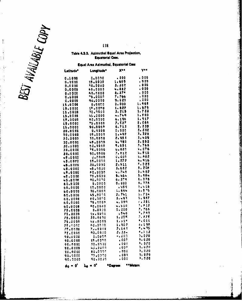
its

Table 433. Azimuthal Equal Area Projectlon,

Equatorial Cam.

I.N -VEqual Area Azimuthal, Equatorial Cae

Lititude' Longitude"

oQO9 o,00no . 000 a 0000, 0o0 15,030 1e .0000.0000 1O.0040 ,,302 0000.0000 0000 be370 0000:000 1540000 7.766 0000,0000 90,0000 9.02 f000

140000 O.lo 0.000 6110 000 ..00o 0 1.6 ,? 911,0000 0, fOU0 5,215 17231,6.0000 4 *0 0 ? t 8001f*O0uo '4o0000 be.19 11

1,0000 ?50000 7,?527 2, 08811.0000 2, 300 5.713 2,3530.0000 001000 000 3.o s30230,0000 1s.000 10 492 363283060000 3040,0 26 911 3v40930,0000 0.00010 4* 50 3, 5230,0001 to.eoo'0 5.651 3,76830.000 s00 , 820 66 07630.0000 90IMO is M12 'se10'.4 .0 000 J.Olfl U , 000 1, A6249,00(00 11,0010 1,272 49 q1b'.1,00 0 3060010 20611 ',02349,0000 5 a I,0 0 s ,682 56,200

4Ato 000 0000030 7~1',.5,0000 70 0030 Sb64 I.Ad8645,000 o0fl 010 6,378 6,3766000 000 0,00060,0000 1 0 00 ,9 .60.0000 30,00'o.1 09 9,6

60.0000 7O, 0 n0 , nIO 4. 0'3bO0000 C a,00 O ,0 7 1,l IF560000 1, ,"0 06 -.05.3000 30,OU T. 4 ?, 87!

710000 3 0000 , a,011

I!, Oa)C An000I0 1.902 199Dfl o0 7J OOl a. e *. 11 2 141

90000 a qO,O0gO 2.33- , I 13,1060O0 t5a a n , 000 go 020

40,0 000 30 n I 10 , 001) o, 0?090,0000 &$j.fl" a 00, , 0209000000 6 a o000 ,0?09O0.1000 ')O, 0 M0 ,00 0,020

0 6 1a 0 qGG00JI caoo

00 0 )4 W O *oem ** -

....

F

~iI119

b I

ii

I

120

-k4 o IWm06

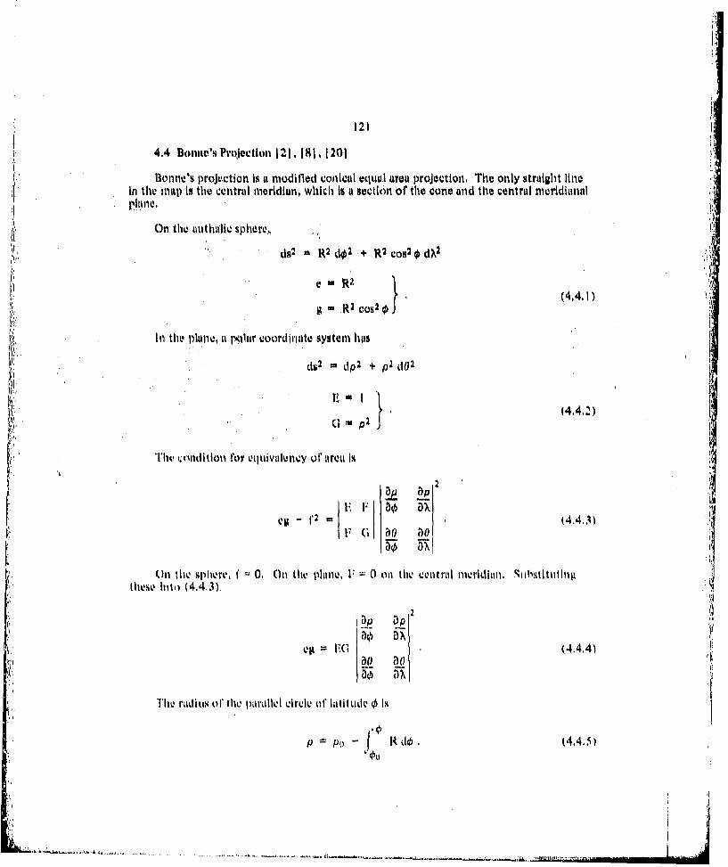
121

4.4 bonneii's Prtkiection 121, 181, 1201 '

B~onne's projection is a moditled conical ecqu.I aroa projection, Tile only straight linep in thf. map Is the central meridian, which is a section or thle cone and the central nmeridiainIl

ds2 P R2 LJ02 + R3 Cs2@ d)X2

(4.4.1)

In tiw plane, it p~fur coordinate system has

ds dp2 + p2 jioa

-Ii 14.4.2)

lll nd(iimt for equ~iivaliui1y ol'arva is

- j2~ (4.4,3)F (1 80 0O

il I lie sphere, 0. Oil the phlne, 1 -- 0 on thev central ineridian. Nubmhstil ing

these Imio (4,4,3) Aep VG (4.4.4)

p Po R do (4.4. 1)

....... ....... ....

From (4.4.5)12

(4.4. M

as 0

Substitutin~g (4,4.1), (4.4.2), and (4.4.6) into (4.4.4).

2

mR2p2 (~

R .CP (4,4.7)

Convert (4,4.7) into an ordinary differential eqLu~tlon, and lIntegrate.

R com p dO

hito C 'S p0 C

- 0 cH + C.p

The constunt c is xcro If the~ condition W~ Imiposed that X. 0 whe'n 0 0.

0 m p (4.4, A)

In Chaopter 1, it was noted that for it conI~u1 projection, tanigent to it sphere,

pcI R cot 0( . (4.4.9)

C'arrying~ out the Integration of (4.4,5)

P Po R(O 00 (4.4.10)

123

Substitute (4,4,9) into (4,4 10),

p = Rcot O- R(0- o), (4.4,11)

The Cartesian plotting coordinates follow simply, with y-axis as the central meridian,and the origin corresponding to 00, from (4,4.8) and (4.4,11).

x - PSsin XRcostl (4.4,12)J

r 'XR cos, 0y = S RcotOn - pos (4.4.13)

where S is the scale factor and X is in radians,

The Donne projection cannot be generalized. It applies to a specific case, with a -peci.fled standard parallel, €o. In order to demonstrate the projection, a plotting table f'or

= 45 has been placed In Table 4.4, 1

The Bonne projection has been used as a military map by France.

The grid itself Is given In Figure 441. Note the curvature of the meridians, and thefact thtit thc piarallels of latitude are concentric circles,

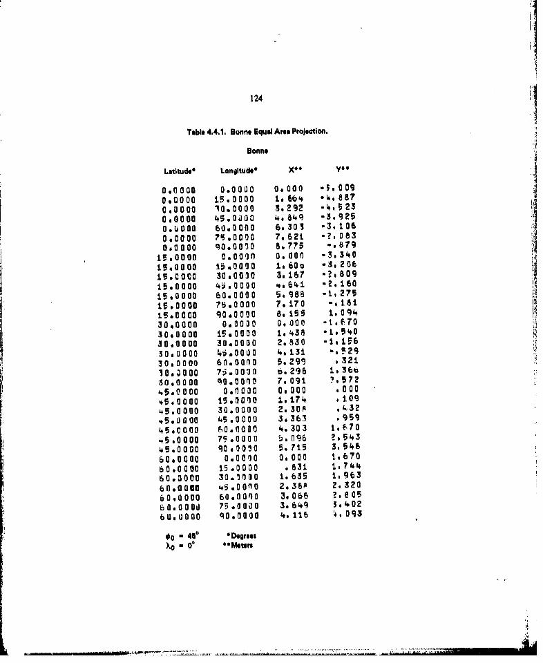
124

Table 4.4.1. Bonne Equal Area Projection.

Bonne

Latitude* Longitude* X** Y**

0,0000 0.0000 00 coo - .009 oo00o 15.0000 1a 664 -. 0 887

00000 10,0000 3292 -4. 523

010008 45. 0130 a ..8'oq -3.9250.U00 60.0000 6.303 -3,1060.0000 ?7,000 7o621 -?,0830.0000 qOOO 0 8,775 -,879

iJ tooo 000 O, aOa I n , 000' - 3@ 340

154,0000 040,0J 1. 600 -3. 206

15.000 30.00030 3.167 -, 809156,0000 4 ,0 0 0 0 64,1 - 2, 1.60

160.0000 5. 988 -t, 275150 0a0 75.0000 7, 170 -. 18115It0 COo qoooooc .iss t, Oc430o0000 0.0030 0. 001 "167030,000 1590 00 1s.438 *L54030,0000 30.0000 2.830 -1.15630,0000 4a.00a0 4.131 5 2930,0000 60,000 o 5.299 ,32 130.0000 75.00030 6,296 1,36630.0000 qo.oOO 70 091 ?.57245#0,o000 0,6030 , 000 .000.150 0000 1500010 1.17. ,10945.0000 30.0000 2,30 ,A 4,32.5.0000 45.0000 3,363 ,959.5.0000 6 0. a 100 4.303 t. 670

'.5,0000 75.0000 b.096 2,543.5.0000 90,0010 5.715 3, 546

60.0000 0.00010 0.000 .670bO.000 15.0000 .831 1. 74460.0080 30.00(10 .635 1,96360.0060 45.00n0 2 38A 2,32060.0000 60.0oo 3v 066 , 6 0560.0000) 75.0000 3.64 €) 4.402bUO0000 q a. 0 .116 4.4 093

0- 45 oDegremeX, 0 "Meters

25

8I

I.

II

Ii

I

lip. 126

4.5 Cylindrical Projection 121, 1151, 1201.,1221

In this projection, the meridians and parallels are straight lines, perpendicular to onleanother. The lines representing tile meridians are equally spaced along thle equator. It re-mains to space the parallels according to the requirement that an area on the projection isequal to the corresponding area on the authalic sphere,

Since the meridians are perpendicular to the equator, and equally spaced, the abscissa is Ix = R 6S e (X.5.f

where S is the scale factor, and X and Xo are in radians. Thle lonigitude. of the centralmeridian Is X0 ,

Consider thle projection from the authalic sphere to at plane, rectangular coordinatesystem, For the pilane

ds2 dX2 + dy2

E

For the sphere

ds2 R2 do?* + R2 C.,32 LdX2

L% R 2(4.5-3)

'l'he cona~itiotI for celuivatieney of' area is. again

y ~ 2

- f (4 5.4)F C' ax o)x

Since both systems aire orthogonal, f= VP 0. Substituting this Into (4.54)

1 2ay by(1 a x

g ic; (4.5,S)3x x

127

IVroni (4.5.1) and onlitting the scule factor,

ax 0 (4.5.6)

'x R (4.5.7)

SubstitUting (4,.2), (4.5.3), (4.5.6), and (4.5.7) into (4,5,5)

ay by 2

R4 cr.)82 80 B

0 R

2

R cos(4.5.9)

Integrating (4.5.9)

y R sill + c (4.5.10)

The constant c in (4.5. 10) canl he zero by selecting the origin oti the equator. Includingthe scale t'actor, (4.5.10) beeomes

y = R * Ssill~ (401

The Same result canl be obtained in a different manner. The area of'thoe vone belowh~i tilLue Onl the autha11l1C SPhere- IS

A = 2 rR2 mill (5.2

The area Onl a Cylinder tangent to this Sphere tit the equator isA -27rRy. (4.513)

Fquating (4.5.12) and (4.5.13)

27rRy =27rR2 sInrk

y = R sill*

128

This duplicates (4,5. I 1). The second method was the one originally employed, and gave theprojection its name.

The grid resulting from (4.5,1) and (4,5.11) is given In Figure 4.5. 1, Observe that dis-tortion is Intense at higher latitudes, and the projection can be of real service only near theequator. This consideration has limited the usefulness of the projection. Table 4.5,1 givesthe plotting coordinates. This projection is also graphically constructed.

This projection can be made oblique by applying the rotation formulas of Chapter 2,If this is done, the area adjacent to the great circle tangent to the cylinder has a regionfairly free of distortion,

--i ._--4

r

129

- - - .

- - in. - - -

. - - S - S I- S - -

I- - - S -

I- ~s - - - -

i

* -S.- - - - - I'F

* - -- -

- - - - - -

- - - -

dJ

130

Table 4.1L1. CylindiremI Equal Area Projeotion,

Equal Area Cylindrical

Latitude* Longitude*X

0.0000 0.0000 0. 000 0. 0000.0000 1060000 is.340 06 0000.0000 60.#0 0 90 Go6V9 0. 000

V0.0000 q0*ootj 10. 019 06 0000.0000 120.0000 lie 35q 0000o0.0000 150.0000 160698 0. 0000.0000 180o10ooo 20.038 0. 000

30.0000 DOOM)l' 0. 000 s. 1i6930.0000) 30.0010 3.340 1 1930.60000 A04(100O b6Is79 10.18930.0000 90.0000 10. 019 3. 18930.0000 120.000 li 6.9 34 18930.0000 120.0000 13.3198 3. 189 x110.0CM 14040000 20s.035 1$.189

60, 0 0:00090 0. 000 so 524600000 100000 So340 So.24.

60.00000 6040000 *6679 So.524.2bOsO. 00000 ioq ±0019 5,524b60000 120.0000 13.31399 So.52460.0000 190.0000 16.698 So.S24600OUOO 180.0000 20 059 5e.52490.40000 060000 0. 000 6s.37890.10000 10.00000 36 340 6. 3789000 000 80.0000 6. 679 6. 3789000000 90.0000 10. 019 60 378a90.0000 120.0009 13.359 be.3789000000 M150910 16.s698 64 37890.0000 180.0000 200.038 6. 374

... .0:......

131

4.6 Sinusoidal Projection 181, 1151 , 1201

The Siuoidal projection, also called the Sinson-Flamsteed projection, is a projectionof the entire authialic sphere, Essentially, It is derived from the Bonne projection by setting

0. Then, p approaches intinity.

On the authalic sphere,

ds2 R2 d02 + R2 cos2 0dA2

e mR2

01.(4.6.1)g m R2 vo08

On t he plane. in Cartesian coordinaltes,

dsl dx2 + dy2

(4.6.2)

Oil the sphere,

I' 0 (4.6.3)

aind along the central meridiun,

The vitul aroa Condition Is- = (4.4

Along(lhe merldian

y Io. 46~

132

Therefore,

LyR

0 4 (4.6.7)

Substitute (4.6.1). (4.6.2), (4.6.3), (4.6.4), and (4,6.7) into (4,635).

R4 CON2 0 84i axR 0

-R2 ()

R cos (1. 8)

Convert (4.6.B) into an ordinary differential equaltion, and integrilte.

dk R con OdX

x - Rcoso + c.

Since x 0, when X -0, c 0.

x X.RS cos 0 (4.0.9)

From (4,6,6)

y - R -S* . (4,. 10)

Figure 4.6.1I Is a SInusoldal projection of the earth. All of the parallels art. atraIghtlinus. The merldIains are sinusoidul curves, The central meridian and the equator are straightlilies.

The Sinusoidal projection is used for geograplLicul maps. The distortion at extrmlela0tItudes and longltudes is simply ignored, A plotting table Is in Table 4.6.,1.

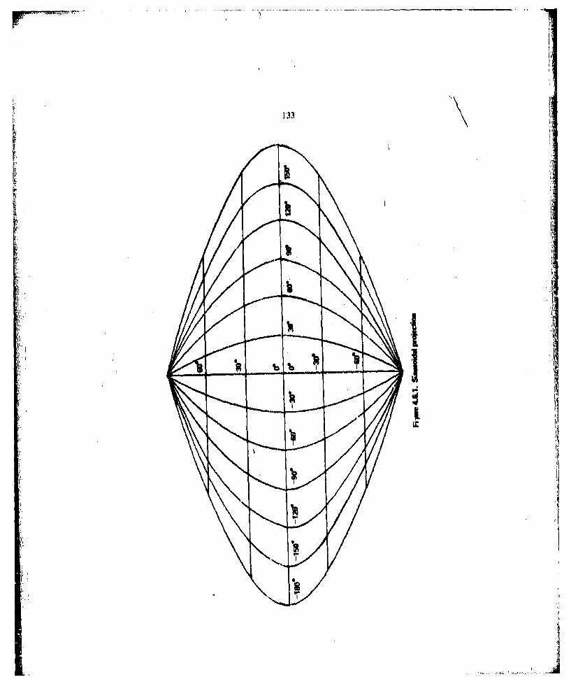
133

i

134

Table 4.0.1. Ulnusoldal Pfojeatlon.

sinusoidal

Latitude Longitude* X*I.o

as.0000 06.100 00.000 06.0000. 0000 3000001 3*34.0 0. 000as.0000 60160000 669 06 000Go.0000 9 U0 a 0 100.Oil 00 00.0003 t20sOO00 13.359 0. 0000.0000 1 040006 16*6908 Oil000a0a0000 180.0000 200.038 0. 000

30. G00D 0.;000 0 0.1000 3.31.03 0.4C00a 30.0000 2.892 301*30-0:900O 60.0000 ~S 8 3o.34030. 0000 90.0000 866T 3@340'306.0000 izasoo0 l±±.b 343430.0000 t1os 0000 14o4161 1*340306 0000 160:0091 0:000 03

360.0000 1000000 0 07.30 6314

60. 0000 .60000 3.31.0 6.679b60,0000 '60*0010 36309 b.679,

60. 0000 120.00o0 66079 6.PiT960. 0000 t50400002 do343 6.67960. 0000 180.0000 , a ±019 666799060000 3060000 as.000 10.0±990.0000 30.0000 -0.000 too.01990.00000 60.0000 -.00 go i001990.0000 90.0000 -. 000 10.60 1990. 0000 120.0000 -. 000 i101990. 0000 150.001)0 -000 LO001990.0000 158.0000 .000 10.019

00 o

X4- Mee

4.7 Mollwelde Projection 115 51 1221

Thle Mollwulde (Fllptic) projection of thll. authalic sphere is derived fromi thle construe-tion In Flgtre 4,7, 1. All of' the meridians tire ellipses, The central meridian Is u rutilinoarellipse or straight tile, und tile 900 meridians are ellipses of eccentricity zero, or circulartircs. The L'rluntor and partillels tire straight lines perpendiciur to the central meridian. Tilecentral ileridianl and tho equator tire trUe 1618th.

The. main problem In this projection Is Splicing tile Parallels so that tile property ofequivalence di area is maintained, To dto this, apply the law of equal surface from theauthalic sphere to the planair map.

The area ot'the circle centered at 0 is

Al 7rr2 . (4.7.1)

This is to be equal In urea to a hemisphere

A, 2irR2 .(47)

Ehquutlng (21,7, I) and (4.7.2)

r2 = .R2 (4.7.1)

r = R. (4.7.4)

Conmkier Figure 4.7. 1, Tlhe at'ea betweeni latitude 0 onl the spherv, and thle equator Is

A -2Trl1 2 sill 0 (4.7.5)

This urea Is eotual to the area AFFI oin the figtuie, For at circle Inscribed within an ellipse,where the radiuis of thle circle is onv hall* of' the seni-milior axis tile area BD1X1 I equals onehtalt'of tho arett AFFlI (i 71. Consider hail' ol'the area hlixiII, flhat Is area ('DGO, This aireaIs composed ol' tfie triangle OCI) and thec sector 01)(1 The area of' thle triangle is

AA X- r sin 0r cos 0

r2sinl 20 . (4,7.6)

Thev area of' thte soctor Is

As (4.7.7)

r136

136

ItI

N;juute thle sphot-1a itrua and the. 11ap a re through (4.7. 5), (4-7.6), and (4.7.7),

27rR 2 sin 4(- r2 0 + 1~ r Sill 20)

ii'R2 sill~ r2 0 +1 r2 sin 20.(..2

Substitute (4.7.3) Into (4.7.8).

irR2 sin o 2 2K2 0 +. R2 Sin 20

7r Sill 20 + sil 120 .(47)

We tire now falced with at traniscendental eqution to be Solved for 0. For~ limited1IMrca graph or 0 versus 0 Can be Constructed,~ as, inl Figure 4.7.,2, and valies ol' 0 read

for givenl Values 0l' 0. However, f'or Computer Implemientation of this liro~leetionl, it Is uecs-sary to resrt to it numericl Solution.

Apply the Newton-Ruphsmon method 1141I, Write (4. 7.9) ats

f(0) 1 S, si(k- 0 - i 0 4.7, 10()

DiITO reiithitling (4.7. 10)

l'(O) -2 -2 Cos 20,. (4,7.11)

The iterative Solution of (4.7.1)) for 0 its a function ol' o is

SubmtittiQ (4.7. 10) and (4.,11 I Into (4.7.1 Z)I 0 ~ In -0 , sil 1011 11 --2 .-+ 2 os,O, I

Micro 0, Is ill radianls. ThIS hlis a rapid convergtence it' the iitial guoss I' 0 Is thv given

Olive 0 Is fond, the mapp111ing equations quickly follow frm iIgure 4.7,1.

y It Ssill (4.7.131

- S;( - 21 vs 0(7,1

.... ~~...... .. ......---... .. ...-

rJ

138

90

80

70

60

40

30

20

t.! 10

a 10 20 30 40 DO W0 70 SO SO

Figure 4.7.2. 09v3 for the Moliweide projetion

JI

where r is given by (4.7.4), S Is the scale factor, and X and W() is in radians, The centralMeridian htus longitude X0.

The result of applying (4,7.1 3), (4.7. 14), and the Iteration Is the grid of Figure. 4.7,3,The (istortion towards the poles Is not as great as in the Sinusoidal projlection, but it is morenoticeable than in the 1-animer-Aitol't projection, The chief use. of' the Moliweide projectionis tor geographical Illustrations relating to area, where distortions tire not disturbing.

Plotting tables for the Mollweide projection are given in Table. 4.7.1. Latitudes 0' to90, in steps ot' 300, and longitudes 0' to 1800 in steps of 30, tire tabulated.

1 140

4bq

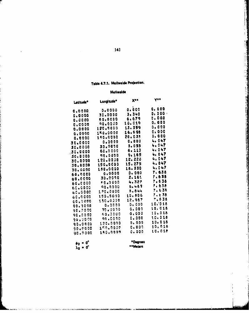
141

Table 4.7,1. Mollwelde Projectlon,

Mollwoide

Latltude* Lonitude*

060000 0.0000 0 00 0, 000

0.0000 30,0000 3o340 0 0000.0000 60.0000 6,679 0. 0co0

o, 0 0 .0 00o to. 0.9 O. coo

060000 120.1000 3.359 0000

0.0000 W04.0000 16.698 o. 000060000 1,i000a0 20.03q 0,000

30.0000 0,0000 a.000 4 047

30.0000 30.0010 305 IsOd.7

.30,0000 60,0000 6,1a0 ,o4017

HAM q 04 a 0 9.165 4s.04730,0000 22010030 .2, 220 46 047

30.0000 MOM ise 275 4, 047

30.0000 180*0000 18.330 4, 04760.000 000000 0.00 7,63860,0000 30.001q0 2.161 7,63

60.0000 00,0000 4.e32P ?036

60,0000 q0l0010 6s481 Fo638

0o a 0000 IP0.000C 8.644 7, 638

60.0000 tO. 00O 10.806 7.18

Go 0.110 t 10,000 12.96? '?.3890.0 000 00o00 0. 000 1011018

9C.,0 0 0. inago 0 1000 10, 018

90,0000 UOOa0 0,000 10.018

9 ,.*Io0 00 inO O 0.000 10.01890,0 a ou 12( ,0 @0 0 04, O00 1 a0 18

90 0000 12 r 000 0.000 10. 0 18

90.[O00 1'O0.000C' 0.000 0.018

)0 - O" *Motm

142*1 4.8 Parabolic Projection 181, 1151, 1221The Parabolic (Craster) projection of the entire world is shown in Figure 4,8. 1. Tile

parallels are straight lines parallel to a straight line equator. The meridians are parabolic arcs.

teThe Parabolic projection can be constructed from consideration atf Figure 4.,2, Lotteequator be four units of length. Then, the central meridian Is two units, A scale factor

will be applied at the end of the derivation to convert the assumed unito to the equatorialcircumference, At present, R Is the radius of the authalic sphere.

Consider the shaded are4 In Figure 4.8.2, bounded by an outer meridian, the centralmeridian, and the equator. The outer meridian is taken to be a parabola, y2 =x/2, with Itsvertex at (0, 0). The mapping criterion requires that one quarter of the area on the tuthalicsphere will be equivalent to the shaded airea between x = 0, and x 2. Thuis, one half of thczone between the equator, and a given parallel, 0, will be

JA (2 -x) dy'0

f fy (2 -2y 2 ) dy

2y - I y3

3 2y (401

The total urea of the sphere Is 41R 2 . S11hstituting this valuec, and y I Iinto (4.9. 1)

,rR2 =4/3 (4. 8.2)

=0.651470.

Next, relate the ma~p ordinate to allthlk laitude. The arua of a zone on the ait halkcSphere from tile uquator to latitude is 2irR2 Sin 1), 1 lall otlthis zone is theni

A ff R2 Sill. (4.8.3)

Elquate (4.8.1) and (4.3)

2y Y'-I, il1 ,s43 ~iR i@ 484

143

00;

I.,

144 I

I,'

II

FN I

1*'-~~*4

~ ~ Im~,.r,.,tr.,,

Substitute (4,8,2) into (4,8.4),

2Y Y3 7 in

-' 3y + 2 sin~ = 0.

A solution of' tis transcendental equation is

y =2 sin 0/3 (4.8.5)

which c.an be yefriied by substitution. A scale- taLctor, S. and radius, R, may be introducedInto (4.8.5) to obtain the ordinate.

y 2S min 01b3 -R . (4.8.6)

''lic abseissat may be obtuined by the follo-wing development. The length ofI a parallelbetween the central meridin and the outer meridian is givmn by

Q 2 - 2Y2 . (4.8.7)

SubstitUte (4.8.5) Into (4.8,7),

22( -4sin 2 0/3)

2 1 + Co

2 2 cos - 2)..8

rii parallels are divied wroplortionally for the IIItersectionls ol, the mleridins. (48o )(4.8.8). and incluiding the scalev actor, S, and radius R.

180

In1 (4.8.9), X Ni Is the di leieuce In longitude betweenl tihe givenl meridianl anld the centraltmeridiatn, inl degrees.

Sinice tis Is an equal area proIection, Its uise is I'r statistical replresntatiott, No at temptIn mde to avoid distortion inI angles and shapeos. H owever, the Listol t inn is les titan InI thle

Moliwide prOJeCtiOmm because thle meridians id parallels do niot intersect at such acuiteiingles, Also, the symmetry and par11abolic, cuIINs lenld a ceitinl iest hetic quality,

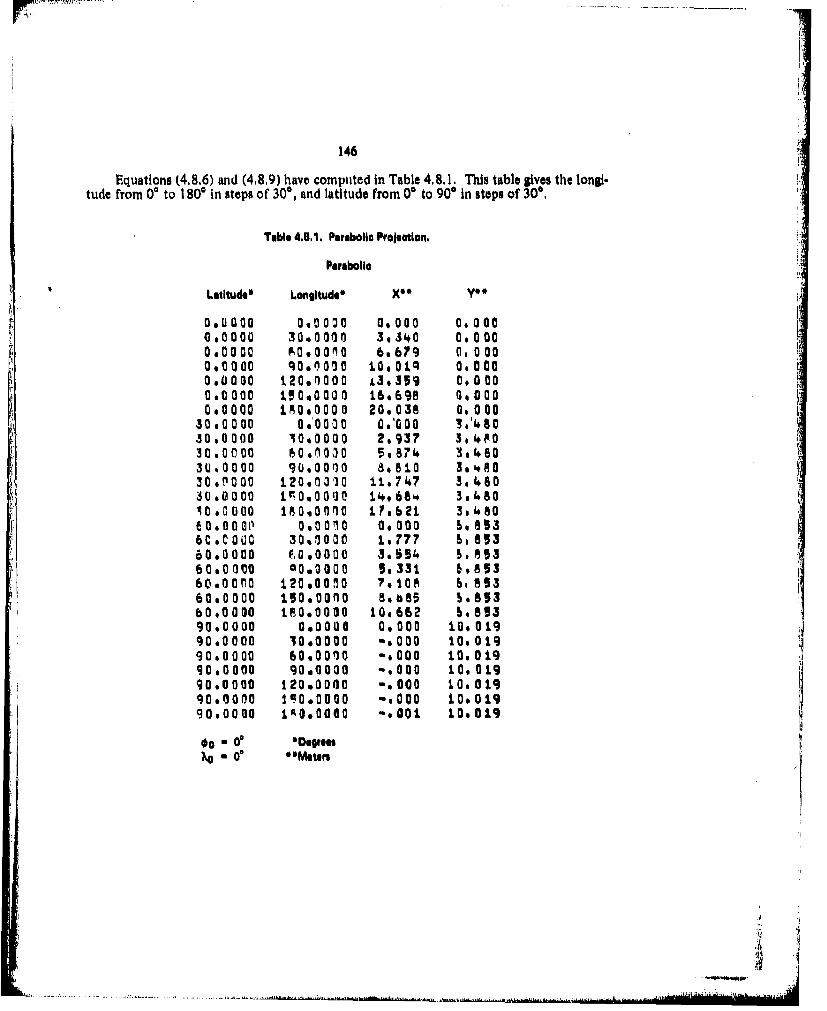
146

Equations (4,8,6) and (4,8,9) have compited in Table 4.8. 1. This table gives the longi-tude from 0° to 1800 in steps of 30° , and latitude from 0* to 900 in steps of 30',

Table 4.8.1, Parabolic Projectlon.

Parabolic

Latitude' Longitude" X'

0.006 040000 0 000 0, 000060000 30.0090 3.340 0 00o0.0000 A0. a 6,679 0 .00OMO qO.8O00 LotDOal 0.000.0000 120. 000 L, 3.359 0 0000 .60 O .. 0* 0 0 0 16,698 G 0000.0000 1 8000 0 20.038 0 000

30.0000 0.0000 .oo0 3.48030.0000 1060000 2,937 3o8030,0000 $040030 S5,8714 3.4803040000 90.0000 8,810 3'8030 0000 120.0010 L-.747 3. 48030 0000 V0.00)0 t',68'. .3480

0 4O000 180.0 00 1r.6621 3. 480E0001 000 0.0 00 5 8936C 0000 3040000 L.777 6. 85360.0000 0.0000 .03,54 $ 8.53150 0 0go C.0000 S.331 6,85360 0000 ±.20.00 0 7 .10aM 6, 85360 0000 1.Ooo0O 54685 8360 aOso 180.O000 10s662 so $390.0000 0.0000 0.000 10.01990.0000 10.0000 -. 000 10. 01990.0000 60.0000 -. 000 10.0t9900000 90,9000 -. 000 10.01990.0000 120.0000 -. 000 1001990q000 1,O.O00O -. 000 10.019900000 AsOGOOMO -,001 L0.019

o 00 "Degrees* 0' 00Me1ters

A°

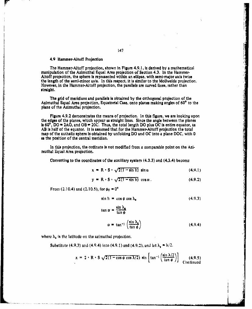
147

4.9 Hammer-Aitoff Projection

The Hammer-Aitoff projection, shown in Figure 4,9,1, is derived by a mathematicalmanipulation of the Azimuthal Equal Area projection of Section 4.3, In the Hammer-Aitoff projection, the sphere is represented within an ellipse, with semi-major axis twicethe length of the semi-minor axis, In this respect, it is similar to the Mollweide projection.However, in the Hammer-Aitoff projection, the parallels are curved lines, rather thanstraight.

The grid of meidians and parallels Is obtained by the orthogonal projection of theAzimuthal Equal Area projection, Equatorial Case, onto planes making angles of 60 to theplane of the Azimuthal projection,

Figure 4,9.2 demonstrates the means of projection, In this figure, we are looking uponthe edges of the planes, which appear as straight lines, Since the angle between the planesIs 60*, DO = 2AO, and OB w 20C, Thus, the total length DO plus OC is entire equator, asAB is half of the equator, It is assumed that for the Hammer-Aitoff projection the totalmap of the authalic sphere is obtained by unfolding DO and OC into a plane DOC, with 0as the position of the central meridian,

In this projection, the ordinate is not modified from a comparable point on the Azi.muthal Equal Area projection,

Converting to the coordinates of the auxiliary system (4.3,3) and (4.3.4) become

x - R. S *2( -sn h) sin- (4.91)

y w RSe S..(/ I-,inh) coso. (4,9.2)

From (2,10.4) and (2.10.5), for 0o 0'

sin = c= os 0 Cos X. (4.9,3)

(sin aa - tan-) (a n € (4,9,4)

where X is the latitude on the azimuthal projection,

Substitute (4.9,3) and (4,9.4) into (4.9, 1) and (4,9,2), und let X, X /21

X 2' R S V/2T'-cos€ cos X/2) sil [tan'I (sinX/2)] (495)Cona tinued

148

00I

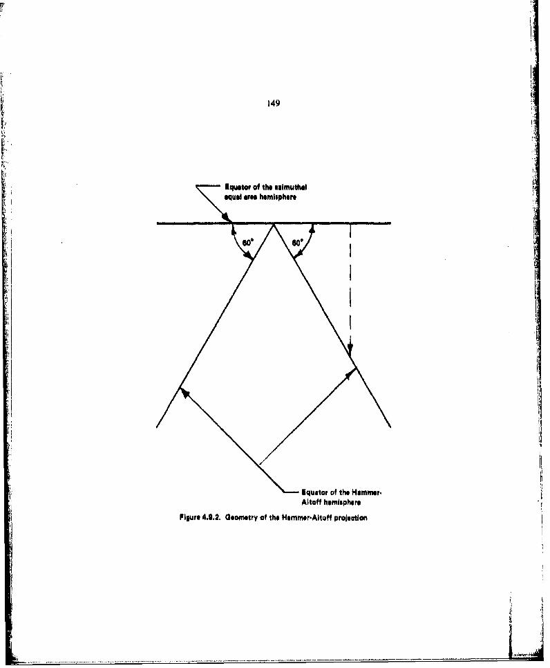
149

Eq4uator of the aulmuthal

Icqustor of the Hammer.Altaff hemisphiere

Figure 4.0,2. Geometry of the Hommor'Altaff projection

-------~ -- -- -

150 '

y -R *S %/2 (1 -Cos 0 Cos X/2) Cos [tail-)~ 2] (4.9.5)

Equations (4.,5) gave tile plotting relationship ol' Table 4.9. 1.

That thle area enclosed by thle ellipse of the 1-lammer-Aitoff projction, correspondingto the entire sphere, Is twice the area of the Azimuthal projection, corresponding to ahemnisphere, follows easily from the geometry of the ellipse with a circle of thle radius ofthe senni-ininor axis insci-lbed 1 171

in Figure 4.,1, the central meridian and the equator are thle only straight lines InI tilegrdd, The rest ot'the meridians and parallels are curv'es, The curvature of the parallels withrespect to thlt. meridians Is such that there Is less angular distortion than appears tit higherlatitudes, and mnore distant longitudes in thet- Mollweide projection,

The Hammer-Aitoff projection Is used primarily for statistical represenltationl of data.Thle distortion that occurs is overlooked.

151

Table 4.9.1. Mammmi.Aitoff Projection,

No.mmer-Altotf Projection

Latitudel LonvltuW e*

00 000 0.0000 .oo 0 ,oo00 UOOO 30. 0000 3.330 .0000.00ou 60.0000 60603 .000U 00000 9040000 94763 P~ooas U 0 0 12 0 00 U a 126 750 .00000ao U 00 o 1 06 00 1.5, 53 1 .000Go.0000 tous.000 tA0 ~0 4 0 .0on

30. 0000 0ia0 0 0 0 6 .Q0 !.0f23 00U000 30. 0000 248 ,V30 0 000 U4.0000 51 905 16 l930.10 000 Uo a a 840 0 '. 5F30. 0000 120.0000 L 1.30 3 .So0 0 0 10 0 U 00 13,6'.0 '4.076Sol.U 0o U.060000 154623 40.60s.U000 n 0000 0f000 6o 3781000 0 3o 0.0000 1 a L 6o.415b 0It0 000 0 0 0aU 0 3 67 A, 2ball.U000 906000D go..$2 6,.714 L

but 0000 12 0000 a0 60,387 6. 98760. 0000 150. 0000 601911 74.351606 UO 000 18060000 CJ.0U2 0 7, P 1290 0 00 0 0.0000 -. 000 1?0fp900 U OJ 30.000o a000 qs n90.U 0 00 oao Uou 0 601 0 02090. u00 U 90.s0000 .000 9 v 02090o U000 i20.uO~o .00 0 690.0U000 150600u' .000 1 p900 0 uU 18 0 0 a0or 0 a01 p

00 - 00 ureXO a 00 *Mtr

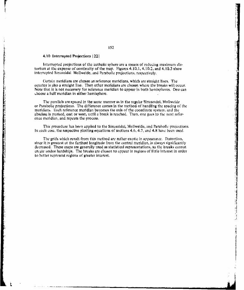
152

4. 10 I nterrupted Projections 1 221

Interupted projec'tions of tile auithalie sphere are a mearis of reducig mlaximum dis-tortion at the expense of continuity of the map. Figures 4.10.1, 4.10,2, and 4. 10.3 showinterrupted Sinusoidal Mollweide, and Parabolic projections, respectively.

Curtain meridians are chosen as reference meridians, which are straight lilies, Tileequator Is also a straight line, Then other meridians are chosen where the breaks Will occur.Note that it Is not neeessnry for reference meridian to appear in both hemispheres, One can

Ihoose at hall' meridian in either hemisphere.

The parallels tire spaced in the sanw manner as in the regular .5intisoidal, Moliweideor Parabolic projections. The difference comes In thle method of handling the spacing of' thlemevridians. LFach reference meridian becomes the axis of thle coordinate syStem1, and thleabscissa Is marked, east or west, urntil at break is reached. nren, one toes to thle next mfler-enee meridia,1 and repeats the process.

Trhis procedure has been applied to the Sinuisoidal, Moliweide, and Parabolic projections.In eauch case, the respective plotting equations of sections 4,6, 4.7, and 4.8 hav'e been used.

Thle grids which result f'ronm this method aire rather exotic in appearance. D~istortion,since It is greatest at the farthest longitude from the central meridian, Is always significantlydecreased. These maps aire generally used as statistical representations, so thle breaks cannotcreate undue hardships. The breaks are chosen to appetir in regions of little interest In orderto better represent regions of greater Interest,

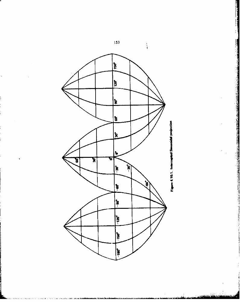
'53

I1

II.

hi

I

It

I I.

I-.

154I

t~l

II I

K

--- - - - .,, ~... ,Ji,...A ~ ~ ~ a.~dhbsa.dt&La.

ir I,

155

:1I

11

.$.

156

4.11I Werner's Projection 121 . 1201

Wirner's projection Is obtained from B~onne's projection by letting 0() 900, From

(4.4.5), we have

4 R do

F~romn (4,4.8), tter substituting (4.11 11)

0 XR cosr 412

I I'the. origin is chosen ait thec pale, the Cartesian plotting equations become

x R1 (7r2- 7r/2

X XCos\y R, ~R(1rI2 - 0) ICo5

The grid corresponding to (4. 11.3) Is In Figure 4.11.1. The only straight line In this cardiolshiaped pirojection Is the central meridian, Note that distortion becomes excessive ait thesouthI pole. and at Inincresed longitudc, fromn the central meridian. The parallels are stillcoIlltric circles. S Is the scalet'actor.

157

Figure 4,11, Warner's projecion

Er-

15H

4.1I2.1I Euinorphke Projection 1 221

Thl unlorphic projution in Figure 4. 1 '.1 is essentially an arithmetic inctun betweentheC inidlW1 and MollwuOie projoctives, This will he tho fltrt projection in whichl onewill hbe UnLlk to obtain general x- and y-plotting coordinates,

mre tirojection is obtained Cor each longitude by summing the distance along thecentral meridian to a giveni parallel Ifor the sinusoidal and Mollweide, and theni dividing by 2.Th'le length of' the, partillel Is then needed. This Is obtuined by requidritg that the ara be-tween thev equator, the central meridian, the given meridian, and the parallel under con-sideration he thle mie on thle hutmorphic aq on the Moliweide or tile sinusoidal projiection,This teias obtainig comparable a reas oin the Moliwle or the sinusoidal by eithier aplunimleter or integrating LI piolynomial which approximates thie meridian curve It is thwnnecessa ry tO Oh tilm tihe X-COOrdinle1S o11 thle Pu inorphic by trial and error withi a planlini-vter, or lilting a polyimnflul curve Thlis is time Con1SUmlilg i.16 and ha not been done InI il- vlport. I iowevmr Ta We 4 12. 1 gives Ithe y coordinates lor' thev Pamorphic projeLtotin

Table 4.12.1., Parallel Spacingil

an the Eumorphic Projection.I

60 1.061190 1,490

159

-I mmoI

160

4,13 Eckert's Projection 1221, 1241

Eckert produced a total of six projections. The one that has received some famre isEckert 4, In this projection, the central meidian is half the length of the equator. FromFigure 4,13, 1, the equator, parallels, and central meridian art, straight lines. The method ofchoosing the parallels requires that the other meridians be elliptical curves,

In the projection, the spacing of the parallels decreases with latitude in a manner thatmakes this an equal area projection, The derivation is similar to that of tile Moliweide.

The area of a hemisphere is

A, 2irR 2 , (4.13.1)

The area north of the equator on the Eckert projection Is, from the Figure 4.13. I,

Al - 2r,2 + In2 (4.13,2)

hlquuting (4.13.1) and (4,13.2)

2irR 2 *2 + 2

0 (2 + (4,13.3)

The area on the hemisphere below latitude 0 Is

A2 = 2 112 sin , (4,13.4)

The corresponding area oil the projection. Including 1i rectangle two sectors, and Iwo triunglos,Is

A2 = 2r rsin0 + ' rsln) rcos 0 +.1r-0

= r2(2 sin 0 + sin 0 cos 0 + ) (4. 13.5)

Iltltatil (4.13.4) and (4.13,5)

2fnR 2 sin k r2 (2 sin 0 +sin 0 cos 0 A- 0), (4.13.w

Fquat. (4.13,3) and (4, 3,13) to obtain a rehttin I etweeii 0 and 0.

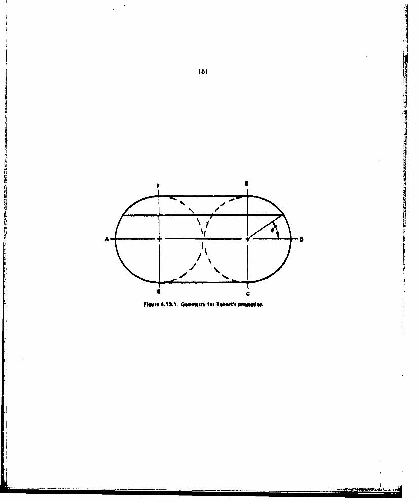
I161

II,

I~. I~IA

p 3

-- I1 N -

I A + DI'

/ \

3 C

P~gur. 4.13.i. Gsontsvy for U~aert's pm~sstisn

162

r.2 (2 + -lsr1 r2(G sill 0 + sill cos 0 + 0)

2 + sinl 2 2sill 0 + sinO 0 os 0 + 0 . (4,13.7)

AnAgain, we have an ugly transcendental equation to be solved for 0 us u Fwmictionl of'O.Anagain, the Newton-Raphson method will produce a result [141, Armed with tis, the

Cartesian plotting coordinate are

x - S - R( I + cos 0)(N- XO)

IT (4.13.8)y = S - R * -sin 0

Chapter 5CONFORMAL PROJECTIONS

Conl formal projections are those projections which locally maintain the shape of anareu on the earth during the transformation to the mapping surface. One important aspecto1' this Is that the orthogonal system of pitrullels and meridians on the spheroid appear as allorthogonal system on the map.

The process of conformal transformation may be accomplished In two ways. One ofthe ways Is to transform from the spheroid onto a fictitious conformal sphere, and thenapply the simpler spherical formulas to transform from the conformal sphere to the plane,cone, or cylinder, The second way Is to accomplish a brute force transformation from thespheroid directly to the, mappin'g surface, Both o1' these approaches will be considered, Thertsults froml either approach will be similar,

The conformal projections to he onsildered are the Mercator, the Lambert conformal,and the stereographic, Three variations of' the Mercator will be discussed: the regular, theoblique, and the transverse. Lambert conformal projections will be represented by one, andtwo standard paraLlel cases, The polar, equatorial, and oblique versions of the stereographicwill be derived,

All of the cofl'ormal projections will be characterized by the conformal relation litro-duced In Section 2.(1. The fundamental quantlties of the flgur of the varthand the mappingsurface will be related by

I= F ( C.;he 7 j

II this eqtillon, tliv capital letters refer to the mappin p surfuce, and the small letterm, to the

chosell figure of the Viarth. Since we will be dealing with orthogolti systems, r = 0.

5. 1 The ('onl'ormial Sphere 1201, 12311,1241 A

lh'e process of producing a coiformal mapping of the earth onto it developabl I surface UIs aided by the fiat that t stccession of con fornial transformations yields t conl formaI ili¢ ,of the original IIrlla oi the fthnal surface. It will be showll that It is possible to project thespheroid conftrnally onto a, sphere of radlius -V/tpTC, dlld ilnlain the quality ofconirm'ltd!ty I'or the subseqttent trans formut lion to the developlible surface.

I ,,['

NEW-~

If one goes through the expansions of this double transformation, and then goesthrough the expansions for the direct transformation, hie will observe that the results areslimihir, but not exact. Thle two approuchies differ fIn higher order terms. Since these higherorder terms contain powers of the eccentricity, e, the numerical difference is negligible, Theprocess of expansion will not be attempted III this Volume, The equations inI til sectionwill be derived in a form convenient for evaluation on a computer, and will be IncorporatedIin the general mapping computer program or' Appendix A. 1.

Once the transformation fromt the spheroidal earth to the conformal sphere Is com-plete, the formulas or trigonometry can be applied to transform from the conformal sphereto the mapping surface,

Fromn (2.3. 15), the first fundamental form of the spheroid Is

(s2 R21 (dO) 2 +I R lkCOS2 0~(LdX

With fiund til 1il ciu.antitICs

v R~ 2 ,(1)

Thv first fundamenital formi of thlt sphere is, fromt (2.3.14)

(ds) 2 R2 (d4))2 + R2 .~2 tl (dMX2

with I'indamlental quantities

C;' R cs1

F~or till's con formal sphere, the c'onfornmal latitude and longitude are deflned to be 1, andA. r eclv y. Tilt radius of' the conformal sphere, is R,

''hev conditions aire ap'plied flhnt the conformal spherical lat1itude IS at f1un001 0t1' of phe-roidal geodetic latituide only, and con formal longituide Is at linear function ot spheroidalIon it tide. Mathematically, this Is stated asN

A cX cl

r 165

Applying the fundamnential transf'ornmation nutrix (2.7.11) to (5. 1 .2) and (5.1.3)

= R2

G c2 R2 coO2

The condition for conformality, as given by ( 2.8 ,2), and applied to the two correspond-Ing orthogonal parametric systems Is

wliero~ m2 is a vonstant.

The fundameontal trunsformation matrix (2.7,11) gives, with the aid or (5. 1.5)

2 2

0 - El (5.1.6)

From gu5.1.31.8

Wr~ite (51 8) inaflotion imie,6).i s omol h oniinofenlrml y

2I

n 166

Substitute (5. 1. 1), (5,1.2), and the partial derivative of k5.1 .3) into (5.1 .9),

~~IR2 = 22 R cosi2 cl )

R~ 1 \~P/R2 cos2

Convert (5.1 .10) In to an ordin ary d ItTurentIalI equation, and take the squaire root, Then, b~yseparating the variables.

m -(1 C Rm

Co s 11 Rp cO0S4(0 (5.1.11)

Substitute (3.1.9) and (3.2.16) Into (5.1.11): to obtain

ca 0csCs (1) -e i~ ~~ 1

COI -C2 )

k! -2 sill'- 0) Cos 0/

111lic solutioni of this ditterL'nial equ1ation is

hI + T!$ c Sil 0 ) + K.1112

Thke c'onstant K is remo1vedl by requ~liring that 11) anl q) are 'oinlcidvlntly equal to ,.ero.Thlus tr-otn (5, 1 .12)

NOte thi this integral Was e111'LulnlL'red biefore, in Section 3.3. for thLe I0Xkodr'OlliL' cUrve olithe sphecroid.

kn 'irder that A mid Q oincidev at /cie ro m tile sconld oI S.3), cI 0. anld

A c

1 67

It remains to lind tho valtie 0f iLe conmtant c for the 1%;rtieular tranisformatiou tronmthe sphieroid to the conformal sphere.

Consider a Taylor's series e'xpansion of the constunt m2 about thec originl. By origin womeian in this development, the latitu~k selected as the origin of the map. Recall that thepartial derivatives or' m2 with respect to X are, zeio. Then,

M2=111?,~ + ( + *, 5.5

Also fromIl (S. I.10)

'<it COS

At the origin tit the matp, m0j 1, by defini tion of' the Conftorma~l projection., Thisspect of map projections will be explored Ili impator 7 on thle theory of distortioin. Con-

sidering (5,1.6) Lit the origin.

Let

cRl .cIR, cos~j 5.8

Taking tho derivaltive of' (he portion ot (5.1.6) in brackets, and siihstitittig (3,2.')) in this

s4i i 1i -I i(P) C o'. (I' (-RI, Sil 0 P.SCos ~ 1) jO( s )2 50)+CS(!iQ

sil (I' Ri l , sill q) llSRpCOS( H/ j si o12

Los()hl Ad* (S

Cos (1) Sill S t(1- 2 j2 ~)-ac2 cos2 1Rp C2os I1~ ell sin2 0)3 2

Substitute (3.2. 16) Into (5. 1., 1u

a(I' C()5 11,11 sinl 0p( I.

Evaluaite (5, 1.20) at tho origin of 'the map,

substitutv (5. 1. 10)into(512)

sill (1)I Cos 4)( c Rnlw Co.% 4) R,1j( sin 0(1CO oRpo COS~ 0 (1S~

TilL next step is to obtain the secund INIrti,11 derivlltive Of 11, 11nd Vquilte this to ze'ro.

T(his IS CCU11111ISh10d by ulSIng (5. 1. 23) to obtain

tanl 0() v t U 1 j - (51tal)

From (5.1.22)

COS C2

Subhstitute. (5.1.24) and (5.1.25) Into (5.1.23), Also, substittute (3,2,9)) and 0.2. 16~),

169 ____ sna '

sill 00 R~ sill tJ)0 /6-- SiJ1)2 -O~

VO~ (I -e-sfjnq,(I- Oo sin2 0a3/ V

0- Se2 1 00)31j~ c

(01 C C2 -J1

COS2 ( 2 (:2-SJ1 0

-08 00l 2 Si,12 0() = I 2)(C2 - Sin12 0()

os2 00 C2 et)82 0 S1,12 00 C1-2 )02 - S1112 00 + 02 SiII2 01

C05 2 + I$ jj2j i12 ~o(I + 1;0%2 0() = 2 C- 2)

e 2( Cos 2 oi)(l +L'Co 2% ) c2( o2

+ +2 (CkIS 4 a -I) C2 ( V - 2)

Q2 -

2 + C2 C084

C + , (5.1.26

'IIQ radius of tiw. con tbrnd spivwre can bo found 1'run (5.1- 23)

sin u __sill '1)

F~romi (S. 1,24)

170

c sinl 4)0 = APn sin 4)() Cos 00 RPn

liminate c between (S.1. 17) and (S. 1. 28).

EquIons11 (5.1-1 3), (5,1.14), and (5.1.26) can be used to convert from thle spheroidalearth to a conformuily equivalent sphere, with a radius given by equation (5. 1.29). Oncethis Is done, the conformal projection fronm thle conformal sphere is relatively easy, Table5.1 .1 gives the conformal latitude in termis of' geodetic latitude for thle WGS-72 ellipsoidwhen ot is arbitrarily chosen as 00. Note that, unlike the developmnent for iuthulic latitude, ~thle conformal sphere depends on at particular choice of origin, 0(). Note also thut (5.12)or the radius otf thle conformal sphere Is also dependent onl this origin, Thus, the rudius of'thle conformal sphere contracts or expands as the choice of' thle origin dictates.

Table 5.1,1. Conformal Latitudeas a Function of Geodetic Latitude

t~or the WGS-72 Spheroid,

Geodetic ConformanlLatitude Latitude

0,0000 - ..00006.0000 6.5050

10,0000 13.011716.0000 16..521520,0000 20.0362

26.0000 32.557130. 0000 39.0855

40,0000 52.1.38945,0000 58.725760.0000 65.293365,0000 71.871060.0000 78.4619615,0000 85,0632

00 0"

171

5,2 Mercator Projection 181, 1201, 1221, 1231, 1241

Theo Mercator projection, devised fIn 1569 by Gierhard Kramer, whose Latin name wasMercator, is the classic of modernl map projections. It wits dorived its anl aid to navigation inlthe. Initial days of the age of'ocean exploration, and has continued It% utility through thle,age of space exploration. The regular, or equatorial, Mercator projection, with its areas of'lesser distortion unorth and south of' the equator, and including tile major maritime traderoute" wits and is a natural vehlicle for ocean navigation, Transverse Mercator projections,with the Lambert conformahl, tire the backbone of' the quadrangle system f'or topographicsurveying. Oblique Mercator projections, with the line of' zero distortion along tlhe noinalstellite, re-entry footprint have beenl Used inl thle recovery charts for the Mercury, Geinli,and Apollo missions.

All three of' the Mercator variations, the regular, the obhiquo, and the transverse,-willbe considered inl terms of' a douible transf'ornmation, that is from thle spherIOid to thle Conl-formal sphere, and thenl to tile malpping surfacC, and thle equatorial ill terinls of' a direct tril s-formtationi of' thle spheroid to the map.

The Mercator projection entails, fin both approaches, a t ransform~ation from thle sphe-roid to a cylinder. Tito Mercator canl be considered inl terms of at semi-graphical technique.One can, with extreme patiemlce, construct at Mercator pr(kiection by at graphical means. Inlfatc t, Mercator, be fore, the developmen~lt of cacuIlus, did it3 that. Tme object ion to ims isthat there is at var'ying projection poinlt. ('1lculations ark! neede,1d to l)cate thle point1 01I'emanation of' the projectioni ray, This i,. shown Inl Figure .5,2. 1. r each andi every latitude,a difffe rent point is neceded as. the origin of' an interior ray which Intersect hot h tie sarflevof' thle spheroid ( or con formal sphere) and t he developable surface, the cyllndir. Thus, thlereasonable aipproach Is to use at mathematical method,

Tmr regular Mercator projection will be developed first for t hi con formal sphivr. lihen.the rotationl forl-1as of, Section 2. 10 (will he applied to produce thev oblique and transvve

case r the regular Mercator protection, let the ('artesian imappi ng coordina tes hev pgi n y

the functional relations,

y YO

Inl partieitilai% the f'irst function is taker ats at linecar combination

x S~- 522

where a Is tine radius ol' the conformal sphere, and S is the skcale fatctor.

'lin deletal forms of the seconld oft (5.2.1 ). 1nind 1..

dIX ans ni

d y Iy(0

172

404

20404

173

The first fundamentul form or the phne is

(ds) 2 = (dy 2 ) + (dx) 2. (5.2.4)

Substitute (5.2.3) into (5,24),

(ds) 2 = (Y) d0 2 + t2S2(dX) 2

, (52.5)

The first fundamental qLUnltites Of (5.2,S) arC

= Id (.2"2

G= 12S 2

The first fundamental form of the con formal sphere Is

(dS) 2 = 1I2 (dO) 2 + L2 os2 (dX) 2 , (5.2,7)

The first fundnmcntal quantities, rrom (5.2,7), are

A a 2 0 1 ,

(5,2,8)g = 12 Cos 2

For the ortIogonl SYStO'IS of tho plane lid the conflormal sphee, the relation ofconformality, tro1 (2,8.2) Is

I (5.2.9)

Sutis tut ing (5.2.0) and 1 52,81 Into (5.2.')).

t12S (112 COS 2 1 I2

dy itsdo C'o~s 0

y = S do t as III tan + + c ,

(5.2.11)

In (5.2. 0), LhoOs' C Su .ch that y -- 0 h r W IlI ' () , Then , v )

174

y LIaS In tanil~ + ~.(..1

Ecquations (5,2,2) and (5.2.11) provide the transformation from the Conformal sphereto the cylinder, or the map. The oblique and transverse Mercator projections will now begained from the equatorial Mercator by utiization of' the rotation formulas of'Section 2. 10.substitute (2,10.4) and (2.10,5) into (52.2) and (5.2.11) to obtain the oblique Mercatorprojection.

x a Scx

sill(N-) O

Lias tanll ; ~ ~ - 522

wherV 01 IS th0 latitude, anld X1, is4 theC longitLlde of the pole of the reference plane1C

y Lis III tanl( + 2i)

2S 11+ sillhI

I~ + sinll sinll + Cos Cos C ( s JI[ .11 Sill 01 - Cos co enCs (N

Thc transverse Mercator projection is obtained ais a spocdal ease of' tlie obliquo Mercatorprojection by letting 01 0 in1 (5.2.1 2) and (5.2.14).

x "is tali 1 -.- -L(.,5tan~ 0

.:i T ) (+ s Coes (N~ X)

Figures S. 2.2, 5.2.3. and S5,2.4 arv specinms of fthe viluatorial, obliquev and transverse IMe rea tor projvetimm:, respectively. Plott(ing tables for thes pr~lL'Li bus tire giveni In Talaes

5,.,5.2.2, and 5.,13, respectively. Note Ilthu tin the equaitorial Mer-cator. thle pa ralles LindmI,-ridians aire st rmight lines, intersecting ait right angk.i. This means t hat thle converAgey oflOw ie ridians does n10t occur, anld dist ortion becomles exce-ssive 111 11 poleward diret ionl. III

tact, the polit o' theC pole is uppuIIoaclilg inifiity. Thius, theV equtatorial projection Is liselossait extremely high and low latitudes. III the transversc Mercator, (lie central nieridiu andthe equtor aire thle only straight lines. I owever. curved meridians and parallels interswctorttiogonally. For thev obliqtue Mercator, there are no sIraigh~t mieritllan-, or parallels. H ow-ever, orthiogonlality Is presenii.

175 1

oil

176

06.

Pipm 5.2.&. Obiqu Mermuo prajndon

177

3w SOt

30ss

30'1

Fliur 5..4 Tionswnom Moresto, pirojuution

17.8

Table 5.2.1. Equatorial Mreator Projection.

Regular Maroator

Latitude* Lonoitudea Xm Yee0, 0000 003 f 0,000 -. 0000,0000 30,0000 J, 340 -000Go 0000 60,0003 6,67i -. 0 Co

s 0000 90,0000 10 09 , 0006 0000 120a0000 13,359 - 0000,0000 150,0000 .L6,698 . 0 00 O00 .,,0000 20,038 ,6b0

30: .00 0000 0,000 3,49,-30, 0000 30,0000 3,3.0 3.146230.0 000 60.0000 6,u? 9 3.48230. 0000 90.0000 t0019 3, 4.230,0000 12040000 L.359 3,4P2a0 0000 15 0,000 i6.698 ."J 4.k 230.0000 180.0000 20036 3 .L, 260. 0000 0. 0000 0.000 8,36360 0000 30,0000 3*3.4 8. 3A360.0000 60.0000 o,6,960, 0000 9 0, 000 10 019 6.36160. 0000 120,OO0 13.359 a " .60, 0000 1 0. 8O00 169698 8.363bO. 0000 180, 0a00 20.038 8,363

*0 * '0 Degrees

00 "Meter

179

Toble 5,2,2. Oblique Mercator Projection.Mercator Oblique Cam

Latitude* Longitude*-30. 0000 00 0000 0.000 l.6e9-30 0000 1500000 8,.S 1.5'?

30,0000 30,0000 2.905 1.139

"30o 0000 45s0000 4,219 ,506

-30.0000 60.0000 5 , 7 ".302

-30s0000 79*0000 6,515 -i. 260

-30. 0000 90.0000 7,54? -20 357-ts* 0000 0.0000 0.010 3s .03

-L±50000 1540000 1.639 3.309

- , 0000 30 0000 3.556 2.767

-15. 0000 45,0000 5090 1.9?'.

"15* 0000 60,0000 6.,''? I. 019

-156 0000 75.0000 70671. -. 040

-1. 0000 90.0003 8.825 "1.1 t

0.0 000 0.0000 0.000 S.6?i

0.0000 15.0000 2.310 S* 314

0.0000 30.0000 4s315 7 , 5

go U OUO0 45.0000 6.093 3.503

0,0000 60,0000 7.5.?7 2.357

O .000 75*0000 8.825 1. 180

0. 0 000 90.0000 10.09 -o000. 0000 0.0000 0.000

15,0000 15,0000 3o081 ?.89

15.0000 30.0000 5541. 65, 79

15. 0000 45,0000 7.380 5.125

15,0 000 60.O00O 6.025 3.715

15.0000 75a0000 10,061 2.40215, 0000 90. 0000 04000 ip 9. 32

30. 0000 0.0000 0000 1.93230.0000 15.0000 4*.61 11.375

30, 0000 30.0000 7,54? 8.86

30. 0 000 4g, 9gb 6974930o 0000 60.0000 10,42t 5*054

30, 0000 75,0003 11.*480 30en?

30, U0U0 90.00000 120491 P,3 7

0 = 4 0 *Degrees)<, 0 0O **Metenl

180

Table 5.23. Trmansvm MeMtor Projeotion.Merutor Tramnne Cow

WNWtde Lonoitude'X* 630.0 000 . 0000 0000 - .400300000 i.o,000 2.688 -?1%*30.0000 30.0000 4e552 -6.20630,0000 +. 0000 5.652 =4,546so$ oo 0000 iO.O00 2,68 -2.95730.0000 7, 00O0 6.583 -1, 45I.30. 0000 90.0000 b@0?9 .000

5f OOU 0.0000 0.000 -5.62145.0000 15.0000 If ot1. -',.324

5o,0.000 30.0000 2.957 "4@546f. 0000 4.0000 3. 26 -R.503

4. 0 000 60.0000 4.s52 -2.35745.0 7500 4.*699 -isi.t495.0000 O0000 5,009 ,0006000000 060000 000 "3s!03bO 0000 15 0000 .946 :3. 36060,0000 30.0000 1.792 P0.95760.0000 4 .o00O0 2.472 -2357bO,(000 60.0000 20357 -1,62960.0000 79.0000 3245 -.83060.0000 90.0000 3.339 .00075.0000 00000 0,000 -1.6897500000 1.0000 o4.2 -16M975. 000 30.0000 .649 -1.45471.00000 46.,0000 1 .94 -1.1805.0000 60,0000 1.454 "o830

75.0000 75.0000 1.615 -.4P875.0 000 90.0000 1670 .c00900000 0.0000 "0,03 ,00090.0000 15.0000 0.037 o00o90.0000 30.0000 0.037 s00090.0000 45.0000 '0037 .00090,0000 60.0000 0.037 . 00090.0000 75,0000 0.037 .00090, 0000 90.0000 0.037 -,C0

V'o • 0° " eeg00 O° *eM

18I

In Figure 5,2.2, the loxodrome (or rhumbline) and the great circle are portrayed on aequatorial Mercator projection, The loxodrome is a line which intersects successive meridiansat the same azimuth, or bearing angle. On the Mercator projection the loxodrome is astraight line, and the great circle (or geodesic) is a curved line, The gnomonic projection ofSection 6.1 has the reverst of this situation. As will be seen, the gnomonic projection hasgreat circles as straight lines, and the loxodromes are curved lines. Thus, by using theMercator and the gnomonic projections together, one can build a series of bearings whichwill approximate, plecewise, a great circle route, This combines ease of navigation with anapproximation to the shortest distance between two arbitrary points. This method is usedfor both maritime and aerial navigation.

The Mercator projectiun, as mentioned above, can also be derived by a direct trans-formation from the spheroid to tle plotting surface, This will now be done to compare thelabor in these two approaches.

From (3.3.1), an element of distance along a parallel of the spheroid is

a cos 0 dWdp -

I

(I - e2 sin2 0)1/ 2

The infinitesimal distance along the parallel of the map is udX, Thus, the scale along theparallel is

dp cos 0adX ( - e2 (5.2,1 7)

From (3.2.16), an element of distance along the meridian is given by

dn a(I - 2) dOdm " (- )~(5.2,18)

(I - e2 sin2 0) 3/ 2

Let dy be the element of distance on the meridian of the map which represents theelemental distance dm along the meridlanal ellipse. The ratio of dm to dy must equal thescale along the parallel, if conformality is to be maintained. Thus, from (5,2.17) and(5,2.18).

dm a(1 - e2 ) d¢ cos 0

'UY dy (I -e2 sin2 0)3/ 2 (I -e 2 sina! )

a(l -e 2 ) dO(I -e 2 sin 2 ) cos (5'2.19)

The distance of the parallel of latitude, as measured along a meridian, from the equator,is found by integrating (5.2.19). This is done by expanding the integral In partial fractions,

t (:d 182

f 0 &(1 -e2) do .

". 1'" ( - e2 sin2 00)5:

fj~ do~@ ~O -ecot 0 o e cos doC 1 -e sin T1+e-"- Mn J

a , __ d + jfo :ecosd; r e cos 0di- { sin (E+ ) 0 1 - ein , -T"in 0j

0 f0 sin *~ # fIf(+

-0 -Cos 0d41 0 c.os 0do2 1 I- e sin~ 2 F; e srnf

y -a n sn + ] In Cos +

+- In 0 - esin 0) In 0n +e sin )]

Ina 1ntan(W +~)+~l t in esn~

I+ gai n

+ (I - c sin~n tan (S.2.20)

Thus, we have in (5.2.20) the same results as (5.2.14) if e is set equal to zero.

The distance along the equator can be found from the integral

x a d,f0

- aA. (5.2.21)

'.

183

The amount of labor in either the direct or the indirect method of transformation issignificant, The amount of computer time consumed in evaluating either set of equationsis similar, The rotations of Section 2,10 can be applied to (5.2.20) and (5,2.21) to obtainapproximations to the oblique and transverse Mercator projections.

5.3 Lambert Conformal 1201, 1231

The Lambert conformal projection is a projection fr6m the spheroidal earth onto acone, which serves as the developable surface. This can be done rather simply by trans-forming from the conformal sphere to the cone. The transformation can also be accom-plished directly from the spheroid to the cone. This second approach will be followed inthis section for Lambert conformal projections with one and two standard parallels. Then,the eccentricity is set equal to zero to accommodate transformations from the conformalsphere.

For the Lambert conformal projection with one standard parallel, the conical mappingsurface is tangent to the spheroid at this standard parallel. The axis of the cone coincideswith the rotation, or polar axis of the earth, The meridians are straiSht lines converging atthe apex of the cone. One of these meridians is arbitrarily chosen as the central meridian,h,, The parallels are a set of concentric circles.

The polar coordinates of a point P are p and 0. The Cartesian coordinates of this samepoint are

x w psin *. S 3. (5.3,1)

y = (pO-Pcog0)S

where p0 is the radius vector from the apex of the cone to the circle of tangency.

Again, the elemental distance on the Spheroid is found from the first fundamental form

(do)2 - R1 (d)2 + I cos2 (d) 2

with fundamental quantities

2.VOS2 (5-3.2)

On the conical surfrce, the first fundamental form is

(dsO - (dp)2 + p2 (do)'

with fundamental quantities

IIi184

V

b

I

185

E' Ij(- '1 2(5.3.3)

'p

Two conditions will be imposed,. One Is that

p - p(,) (5,3.4)

and the second is that

0 ctX + C2. (5,35)

From (5.3.5)

88

From the fundamental transformation matrix, (2,7,11)

E " 2 E'

(5.3.7)2

Substitute (5.3.3) into (5,3.7)

2

(5,3.8)

LO P2

Substitute (5.3.6) into the iecond of (5.3.8).

G - cp2, (539)

From the condition of' conformality (5, 1.9) for two orthogonal systems.

1P' (802(;

= ...... a in2 , (5,3.10)

I m

'- .... .... ...... . : :, ' ; - " .' .c 2 ,

186 *1Substitute (5.3.2), (5.3.3), and (5.3.6) into (5.3, 10),

tap\ opM2..

2 = = in2 (5,3. I I)

Take the square root of (5.3.11), and convert the result to an ordinary differentialequation

dp R c dO(p Rp Cos 0 '

The minus sign is chosen since p decreases as 0 Increases,

Equation (5,3.12) can be integrated by the method of Section 5.2 for the Mercatorprojection to obtain

I e inInp *-Ct In ta +ai

+In c3

A "I/2 "_ eslnj, (5,3,13)

p {3tan ( __i i

The constants cl, c€, and C3 must be evaluated now. First, fr'm (5.3.5), it is required

that 0 = 0, when X a 0, Thus, C2 - 0.

Next, consider C3. At the origin of the Cartesian coordinate system of the map (00,h), the cone Is tangent to the spheroid. Thus, similar to the development of Section 1.6

P0 m Rpo cote 0o. (5.3.14)

Evaluate (5.3.13) at o, and equate to (5.3.14).

IK !LOII +e*sin#oe/Epo cot 00 C3 tan

4 2 *sin 00

Rpo cot #o--,(5.3.15)

esino/)}c [tan. ca

187

Finally, from (5.3.11)

tp, COSRm cos5' (5.3.16)

At the origin, as will be treated in detail in Chapter 7, nio I. This implies that (8m/8O) o 0.Differentiate (5.3.4), and evaluate this at the origin.

am (O) I + Rm sin 0 0

RE / o 0i 2 -o

C1 + Rpocos - 0. (5.3.17)

From (5.3,12)

C1 O O RMO

P) p Cpo o (5,3.18)

Substitute (5.3,18) into (5,3.17)

CPoRMo CleoP Ro sinl 0o- cos o + R 0 cos 0PRp Cos 00

€l 0 sin0o, (5,3.19)

Substitute (5.3.19), and (5.3.14). into (5.3.15)

PO (5.3,20)

{(tan (A~ - L) (I+G sin 0)

Substitute (5.3.20) into (5.3.13).

f/ 2Iesinlj"2

tan (- )(1 +1esinP Pu*a\I_4_s~n~~~2 (5.3.21)

to ( W o00 1 + esin~o) JSubstitute (5.3.19) into (5.3.5), and recall that c3 -0.

/,

I188

0 X sin 00. (5.3.22)

Recall from Section 1.6 that sin 00 is the constant of the cone,

Equations (5.3.21) and (5.3.22), in conjunction with (5.3.1) and (5.3,14) give theplotting equations in Cartesian coordinates. Table 5.3.1 is a plotting table for the Lambertconformal projection with one standard parallel based on an origin of 00 - 45', and )W - 0*,

The Lambert conformal projection with one standard parallel may be converted to aform for the transformation from the conformal sphere by letting a 0 in (5.3,14) and(5.3,21).

Po a cot 0o (5.3,23)

P- tan ( (5.3.24)"~{tan

0

Equations (5.3,23) and (5.3.24) are then used in conjunction with (S.3.1) to produce theplotting equations.

The next step will be to consider the.Lambert conformal projection with two standardparallels. This projection has had considerable utility as aircraft navigation charts, and hasbeen used for star charts by the U.S, Air Force. Again, the meridians are straight linesradiating from the apex of the cone, and the parallels of latitude are concentric circles.

Let tho two standard parallels be chosen as 01 and 02, where 02 > *1, Then, from(5,3.16) and (5.3.19)sin 0o 1

m - 'l Rp, Cost

(5.3.25)sin 02= P2 Rp2 cos* 3

p! Rp COS 02

P2 RPI Cos ' (5.3-26)

P2~~~ Rp S0

. ...... .... I........-........I........ .......

189

Table 5.41. Lambert Conformal Projection,One Standard Parallel.

Lambert Conformal, One Standard Parallel

LatUde Longitude* * *000000 000000 DOMF0 -4 I8 60.0000 158003 2.186 -640.0000 300800 4.297 -4*GPI000000 45.0000 60261,37000.0000 60.0000 8.011 -2s3770.0000 7 0000o 901*880.0000 90.0000 10#640 1 1

1544000 040030 0.000 -3.47015. 0 000 1540000 1.81p -3.30215.0000 3000000 3.567 -2.8021560000 '560000 5.198 -169saLb.0 00 0 60.0000 b65t -.8881660001 75.0000 70877 s46015.U000 9040000 8.$334 2.0OIL3000000 0.0021 0.000 -1.685MOM00 19.0030 1.486 -1*54530.0000 30O00 2 92 1 -1.13630.0000 45.0000 4*296 s730.0000 60.0000 5.446 .431MOM00 75.0000 6.449 1.535

30.0000 90.0000 76232 20MOS* '.5.000 0.0000 0.000 .000

45.0000 1540000 1.176 .10945.00 30,0000 26312 4145.0000 4500300 303b9 .96045.0000 b0.0000 4.310 1.67345.0000 75.0000 so105 2.5474:oo0 00 0 90.0000 5.724 3.65260o00O0 0.0000 go.000 1.600O60.0000 1500000 0665 1.77060.0000 30.0000 W.O0 2. 00860.0000 45.0000 2*477 2639660.0000 60.0000 3.170 2.92060.0000 75.0000 So.?54 3a56360.0000 90.0000 4.210' 4.303

X 0 Go Meters

190

From (5.3.21)

shn.0I + e sin0 1P1 (4 -) (T- esln-j, (5.3.2,)Itan (Z Y) (T -- + O

From (5.3,26) and (5.3.27)

~ ~o'i { (r-})( :n:)/~A\ Ij +einAo/2

sin~oln {I + e Sinl 2~ 1

ttn- e sin 011 s/2

In R 2 cos 2/sin 0o e -

In{ tan(n-") ( st-' in /- } (5.3.28)tan + sin

So fur, the conical surface has been considered to be tangent at the central circle ofparallel, In order to require secancy at , and , 2 let ni = in (5.3.25)

P1 sin-o ,p sin 02Rp cos~I R 2 cOS 2=

spi sin¢n = R2 cos /In ,(5.3.29)

P2 sin o (R2 cos 02

-Z-T esn0

:- -' " ' " So ........ t" conical.. surface....... ha .......... .co sdee t"o-" be tan en at th cenra circe..

191

In (5,3.29), sin 0o, as defined in (5,3.28), applies. From (5.3.21)

tan , + °.i 0 ")P1 O

(5.3,30)

L f 00(~ 1 + *sin Oo,, , tan. (3 T) -- ,-srn' * 0,-0" l ,..o

Substitute (5.3.30) into (5.3.29).

___________ 12 ~l

01 1+ e sin OtP " 0 - ' sn , -"" 1"CO"'

( \1 - e sin 0o 1}

LetPO

I + e in. o/tan ))(14 L2\1- sin 00

-R p j c o s o9/ 5 3 3 1 ' )

sin o tan T- ) " (1 - e sin

In a similar manner

Rp2 COB 02

(-W+ e sin 02 sf2

The polar equations become

0 = XsJn o

-'(4 - e sin tan L} (5,3.32)

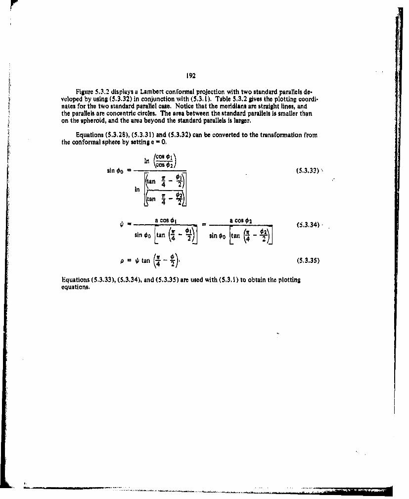
192

Figure 5.3.2 displays a Lambert conformal projection with two standard parallels de-vcloped by using (5.3.32) in conjunction with (5.3. 1). Table 5,3.2 gives the plotting coordi-nates for the two standard parallel case. Notice that the meridians are straight lines, andthe parallels are concentric circles, The area between the standard parallels is smaller thanon the spheroid, and the area beyond the standard parallels Is larger,

Equations (5.3.28), (5.3.31) and (5.3.32) can be converted to the transformation fromthe conformal sphere by setting e = 0,

I/Cos 01

sin o (5333)

tan 4-

p i tan ,,- ,(5,3.35)

Equations (5.3.33), (5.334), and (5.3.35) are used with (S.3) to obtain the plotting

equations.

rT

41

JIV

194

TaMe L..2 Lurn~t mflGnwmal Pret~domTWO stodud PwalIob.

Lanm~b cAoftmi, Two stuidad Nvdleb

Lotus Lorootudo* Xo*vo

Igo.Coco 3000000 w. e

15000 a1.5.0000 be.961 6221

30,0000 05.0000 as.1 1.1.8900

"k 30.0000 30.0000 2S27 20706

30500000 4500003 4010 to.t69

OsO.0OO 1'5.0000 1*0342.0

45.0000 30.0000 2.031 60

1.50130 ~ .0002.95S 3.02945sODO 50000 0613. 662

4booo0o 6000090 37

60.0000 960000 04000 4r, 131

60000150000 .soo 669 a9

b0.0000 3MOM0 le315 108

60.0000 4. .0000 1.915 *P

60.0000 6000000 2*4485*09

164i00a0000 DOM.300 o 5 -

75.0 1~0000 .~oo 329 08

7boo0oo 3000ooo osio? 60ce

7540000 ios.0000 .942 60730

Too.0000 60.0000 1.204 613

30 *D#u..03 2 0 *f

),00

195

5.4 Stereographic Projections 1201, 1221, 1231, 1241

The stereographic projections entail the transformation from the spheroid to the plane.Three variations of the stereographic projection will be derived. These are the polar, theoblique, and the equatorial.

The stereographic projection may be considered as a purely geometrical projection,This is illustrated best with the projection from the conformal sphere to the nane tangentat the pole. The geometry of this projection is given In Figure 5.4.1.

The plane is tangent to the sphere at the north pole, N. The rays emanate from thesouth pole, S. The principle of the stereographic projection requires that the projectionpoint be diametrically across frorh the point of tangency. A typical ray from S to a point Pon the earth is transformed to the position P' on the plane, Thus, the entire projection canbe derived by elementary trigonometry. The same is true for the spheroidal case, only thegeometry is considerably more messy.

The approach in this section is mathematical rather than geometrical. This approachbrings out the quality of conformality immediately, We will consider the plane as one of thelimiting forms of the cone, and then apply the equations already derived for the Lambertconformal projection with one standard parallel. This is done by letting the parallel oftangency for the spheroidal case shrink to a polar point of tangency in order to derive thepolar stereographic projection. To this end, let 00 " 90* in (5.3.19), (5.3.22), (5.3.14), and(5,3,21).

sin 0 1 (5,1)

(5,4.2)

P0 RpO cot 0

= a ,cot 0o (5.4.3)

and

(t )(I + esin .612

acot0o tan 05_ 'V( - e s n/ L

ta (W+ - (I 1

tan (I e sin ' a |

tai 5X .... i4 2/¢- - (5.4.4)

ta O

196

U.I.OMM f~rdw 181 OVO ic R!RIO

197

In (5.4.4), take the limit of

ton 0o

as 0o approaches 90* ,

. tan +o - L

4

L L[1 + tan 00/2'.t00 tan 0/ 2 tan Oo/2

L 0 +tano/2j 2

Substitute (5.4.5) into (5.4.4),

2a /I e esin

The Cartesian plotting coordinates for the polar stereographic projection arc

x -psinO 4(5.4.7)

y - -p s coi.

Equations (5.4,7) are evaluated using (5.4.3) and (5.4.6).

Equation (5.4.7) can be converted into a transformation from the conformal sphere tothe plane by letting ea 0. Then

p - 2a1 tan W ) (5.4.8)

Substitute (5.4.3) and (5,4.8) into (5.4,7).

x - 2atan - si S,4)

y - -2a tan - cos X

Figure 5.4,2 gives an example of the polar stereographic projection. Note that themeridlans are straight lines converging on the pole. and the parallels are concentric circlescentered on tle pole, The spacing between the parallels Increases as one goes towards thleequator, Table 5.4.1 gives the plotting coordinates,

198

le

PFpu 5.42 Pghv uitMmspb pv~de.

199

Table 5.4. 1. ft~morm" hleP*sld P"I OW.6qq..ginhoe Pv1jb.Uo, PsI. Cm

640000 064801 1107146 cases0.1006 150000 18.300 3*316.0000 30.0011 116410 4170.0606 '.sMON Moo, as."I$*lose 606000 6.31 Itself0;,0000 790060 $also 1261pS000000 90000 -01908 124711.

1560088 0.060 9.771, 00061160006 15.0000 9.1.39 tells15.06000 30.0006 06.1 1.6411.0000 15.003 6.910 6.916is's0 00 0 * 0.0000 4.*66 6.1.31.0005 71.00001 loose 9..3915000 9060000 mo600 997733101 0606 7.34 6000310000 1540003 7.111. 1.9630.0000 30.000 6.176 1666310.0001 451.600 $.360 votes8000 60.000 31.403 A.3730006 75*6010 14916 76114.30.1O00 90.0630 Moose 7.31515.0000 0.00leo0 5.291 060665000 1545418 5.111,450003 30.0660 . 456 t46.

'.5.3000 450016 1.71.1 3.71115.0006 0100 1.669 1.5625.00006 ?98006 1.149 5.111

15.0000 960010 &*oil 16291,4.0000 0.6016416 0.060606.0000 1560431 1.810 $so?6406001 30.001 a 096 r 1.71160.00061 400.00 20613 l.e43160001 6000600 1.713 3.96766.0000 75*0608 .0667 3.316$0.0066 90.0060 -0600 3.1.26J1,60006 06006 1.465 loo0375.6000 1540060 10627 04,4679.6006 Moose6 1.1.59 .613ri.6600 '.5.006 19191 1.1917161000 60.0008 .31.3 1.1.997164005 941.08 .1.36 101?79901600 1040366 MOM3 1.0660909000 0.06661 ago$$ 6.0096000 15.0066 moose m.o"

$$*fees6 $000100 MOM6 .0060

96.0636 10.04413 .0 wool@

Oo ho Ntk*0' '03m "Mefnn

200

The oblique case for the stereographic transformation from the conformal sphere tothe plane may be obtained by applying the transformation formulas of Section 2. 10. Thelatitude and longitude of the pole of the auxiliary coordinate system is #p and p, respec-tively. Write (5.4.9) as

x *2a tan Z~-4 sin a(5.4,10)

y~~ ( .u-jta(-)cosf

Then. from Section 2. 10.

a tan sin (X - p)}

It " sin {sinOn + os cosop coi(X- .p)}. (5.4,12)

Equations (5.4.10), (5.4.1 1), and (S.4.12) will then produce rid such as the one InFigure 5.4,3, The only straight line In this projection is the central meridian. Table 5.4,2Is tho plotting table for Op w 45.

The equatorial oase follows when Op - 00 in (.4.I 1) and (5.4.12). These equationssimplify to give

a ta ,in (X- XI t(.4.13)

Ih - sin ' (col 0 coo(X. -A )} .)

Figure 5.4.4 shows an equatorial stereographic projection. The equator and centralmeridian are the only straight lines on the grid. The other lines are arcs of ellipses. Theplottlnl coordinates are in Table 5.4.3.

The stereographic projection can also be derived for a transformation from the con-formal sphere by a process similar to that introduced for the gnomonic. azimuthal equi-distant and orthographic projections of Chapter 6.

_____________ ,I.

203

rr

A

B II'I

j

202

TabbL .2.IN ltmrpe sPraJ9lm., ObNqueStevopahIG Pig)" on, Obliqe cm

40:000 901

00000 70.0000 6100l I520.0000 4*00is?60t504000 0G0000 4090 wtl0.0 a000 1;40000 1071 -103001.s000 0 3060000 271 e

45.0008 3.416

too.0000 70.0010?1II M B:00I 00000030#0000 1540000 .4MOM00 30.0000 IS932 01619?30.0000 "SeO0G0G 40.S? 41690.M0.0000 Oofod'oo 5.064 f30.0000 7300004 7.ll? W.AJ.30.0000 1040000 .0 3:332'.5.0000 040040 04000 d'.5.0000 105.000 1.277 a11'..OCOOo 400000 3441 100

.4be0000 600000 4*464' 10422165.04000 75.0000 54.11.1 t9 61'5.0000 '1000000 6,,013 4639?60630000 0.600 Ogl0$ 1.0?,b0.0000 1560000 0645 10766b*4000o 30010 1.60? ID.056600.0000 45*0000 24*21 2.1.01600.0000 600600 3.067 301016600,0000 79.0000 $.bib 3*lftl00.0000 90.GUOO 3.056 4094?50.a000 0.0000 0.060V #a17600000 i~s0060 .1.19 3.1.7271.0000 M0.00 66 3e633Y5.0000 4.5.0603 Lola$ 3.396b0.000 0 00.0000 1411 4.113M5.0000a 79.0000 1.51.3 4.6

a .000 98.0000 1.962 .1??90.0000 045ooo ago0g.IP90.0000 iv.eou .6 0,11 e4f916.0000 30.0000 aso00 1624i490.0000 49.0061 "sol0 .744944.001 00000 fit010 9.614900006 7500000 64040 b*14960000 90.0011 Wool$ so01 p, I

09 Or Xo Me0 *ogu **t,

203

Id.

Flpav 14.4 $sWFUU*N p*.osm', aetoud am

204

Table 5.4.&. Stesreorepte Proectin, Uquatoial Cms.

Sterowphic Projection, Equatorial Coo.1atituds* Loneltuds y.004000 0.0000 as 000 Q#onO0.0000 06~0000 t e W9 0o aao06000a 30,0000 30,4 0. 000Of.0000 4i,0000 5.284 0. 0000. 0000 '.O*J000 906 0.000D.o 00 0 .0.0000 t2$?51 0. 000

L5600 GOOD0 0.M v000 toU79lbe Ouuo isle 000 l.ob401 a0 00O 30.0000 3039% 1 SOP

M .0000 6000000 at9V 226IS 0 0 0 150000 9..122 as bi.1ibe uQ q060000 12.322 60

30. 000') 1-3.0000 1.6? 'o?

30.0000 MUDDOO 39.06 6IM000"50000 8.4%a 5.210

30o'0000 ')0O0000 1100'.&$?'.6.000 7100o00 0.000 52301.0000 3000000 IL.77 5.6'

45s.0000 60.00aCa 00040 1714

45600090 7%00000 7.565 766V4"3Qo91.0000 9.023 4P

60.0000 0.0000 04 uOO 6t606000aosca I it.00 .13 00ba0 o0 a 30.0010 2.22578Vboo.0000 4q 0 0 0a 36413? 6 41IA2600.0000 6900000 4v ol asidboo JOOO 7'360900 IetP 00blis 0000 9000900 6.17 a1,o0'.??'dSOO 0.0q0000 0.040647176.0000 15.0000 .*664 9.6'WFT a 00 11.0000 1*348 lot asoHE a0000 4.5.0030 L6471 10641b?50 a ag 60.0000 2*332 1069t0?SS.0000 7960000 of 6 1 6 1-75 6. 0900000 goioo so31 M2.322900 0 U0 0.0000 0. 000 12.75?54060000 00500 .5000 12675?9boo0od 30*0000 as.OD000?z9060000 '.5.0000 -. 000 tsq90.00 go0d.0060G -. 000 12o0gb90.0000 7400000 -. ,000 1,vt90.0000 90.0000 -.000 tpe T'6

00 it O o e Dor 0.gu. *Qhs

Chapter 6

CONVENTIONAL PROJECTIONS

Conventional projections are those which are neither equal area nor conformal. As wasmentioned in Chapter 1, this is not a derogatory term, The conventional projections wereproduced in order to preserve some special quality which is more important to a particularcartographer than equal area or conformality, or to present a projection which is eithermathematically or graphically simple. Since the category of conventional is a catch .-all, itis to be expected that there iq a wide variety in this class of projections. This Is true, Someof these are really of historical interest. Some are simply convenient. Others have provedto be cartographic work-horses,

The most useful of the conventional projections are the gnomonic, the azimuthalequidistant, and the polyconlc, both regular and transverse, The simple geometrical projec-tions of the conical and cylindrical, as well as the orthographic projection of the engineer,are examples of strictly geometrical approaches to the problem. Of mainly historicalinterest, are the Van der Grinten, the plate carr6e, the carte parallelogrammatique, the Gall,the Murdoch, the Cassint, and the stereographic variations such as the Clarke, the James,and the La Hire. Finally, there are such mathematical endqvours as the globular,

Clearly, the conventional projections provide maps ranging from the most utilitarian tothe unique.

6.1 Gnomonic Projection 181, 1201

The gnomonic projection requires that the transformation of positions on the surfaceof the earth onto a plane be based upon a projection point at the center of the earth. Thename comes from a gnome's-eye view of the world. The gnomonic projection can be apurely geometrical construction. However, we shall use spherical trigonometry to obtainthe oblique gnomonic projection, Then, the two limiting cases of the projection, the polarand the equatorial, will be obtained by particularizing the oblique case,

Figure 6.1 I portrays the geometry required for deriving the oblique gnomonic projec-tion, Let a plane be tangent to the sphere at po'nt 0, whose coordinates are (00. NO). TheCartesian axes on the plane are such that x is east, and y is north. Let an arbitrary point P,with coordinates (0, X) be projected onto the planL, to become P', with mapping coordinates(x, y),

Define an auxiliary angle, 0, between the radius vectors CO and CP. From the figure

OP' = a tan (6.1.1).

205

206

PI.

Firgw. 0.1.1. Goonwvy.fur the oblique gnomonic projection

207

On the mapping plane, define the second auxiliary angle, 0, which orients OP' withrespect to the x-axis.

xL a OP' Cos 0 (6.1,2)Substitute (6.1. 1) into (6.1.2).

x a tan ,P cosn 0

* sPCome (613Cosn~

Also,

y OP'sin 0 (6.1.4)

Substitute (6. 1. 1) into (6.1.4).

y = a tan ~'sin 0

a sin~ sinG 0615

It is now necessary to find and 0 In te~rms of 0. 00, , and X0. From Figure 6.1. .1,by the use of the law of sines

sin 0,- )0 ) si(96-0sin /i sin (90* -

Con 0

sin 0I com 0 *sin (X- X0 ) cos~ (6.1.6)

Apply the law of cosines.

Cos Pcos (90 -$0 ) Cos (90 0 -)

+ sin (900 - 00 ) sin (90* - 0) cosn (X - Xo)

sin 00 sin0+ cos 00 Cos 0Cos X - X0 ) (6.1.7)

Apply equation (2.10.6)

sin ~,cosn (900 - 0) sin (900 - On) cosn (900 -

-Con (90o - 00)+ sin (900 - 0) Con X - O

208

sin ,isinG CO coo sin

suin 0 s0 c~o(X -X0) (6.1.8)

Substitute (6,1.6), and (6.1.7) Into (6.1.3), and (6.1.7) and (6. 1.8) into (6, 1.5).

aS con 0 sin (X -NO

X sin 00 sin0+ Cos 00 Cos0 Cos (X- Xo

YEaS~cosOO sino-sinoo cos~cos(?X-X 0 )I 619S sin 00 sin 0+ cos 00 cos 0coso.- ) (6.1.9)

Equations (6.1.9) are the plotting ev~ations for the oblique gnomonic projection, Thegrid resulting from a selection of 0 - 45 , and X0 0* Is given as Figure 6.1.2. In thisprojection, all the meridians, and t~ie equator are straight lines, since they are great circles.An arbitrary great circle distance between points A and C, on the figure, is also a straightline. The loxodrome between these same two points appears as a curved line, CompareFigure 6.1.2 to Figure 5. 1.2 for the equatorial Mercator, in which the situation Is reversed.Table 6. 1-1 has the plotting coordinates.

To find the gnomonic polar projection, It is necessary to let 0 * 90' In (6.1,9).

aScos 0 sin (X - XO)X sin 0

-aS cot~o 0 n( O

as cot 0coou(X -XO) (..

A polar gnomonic grid Is given In Figure 6.1.3, and based on (6,1.10) and (6.1.11). Inthis case, all meridians again are straight lines. The parallels are concentric circles, whosespacing Increases as the latitude decreases. Thus, the distortion becomes extreme as theequator is approached. The equator Itself can never be portrayed on the gnomonic polarprojection, since a ray from the center of the earth to any point on the equator will beparallel to the projection plane. Table 6.1.2 is the plotting table for the polar projection.

4

209

Figw.s 6.1.2. Ohjiqvs gnomonic ~o*t~n

210

TAB. 6.1.1. mnsme~io Poola. OMNI wn.

1560000 060000 0.000 -. 6

1560000 1960000 14892 -3*00

15.0000 30,0090 3.97? -34,364lbs a0Do0 40sOIOO 6.51 .7

30.10000 90090 0.000 -1.70To3000015.0000 1.413 -1.600

M O M00 300000 3.125:1 0730.0000 W,.OO 0 a 0645.0000 0.0000 000.000 S

4500015.0000 10160 .111

45.0000 30.0000 247.5'..00045.0010 3.736 1609

60.0000 I0.0000 0.000 1 * 7

60.0000 3040010 1065 160116

7500000 15.0000 .497 3.055

*79.0003 30.0000 .981 3,9767500000 4560610 1&43? 4o346

211

pion, CIAL Pone vemnie pigdw

212

Td"e 6.1.2 GammSUII PVI~jNVA, Ps. cm.

Gnm tIPd Pr~bOmn

30a.0000 0.0000 0.000 buS Od.S30*0040 04.0000 2.699 -10667t30.0000 30.0000 6521' -9696730.0000 45.0000 7.812 -'7.81230.00000 6860000 9056? -9a524.30.0000 7660000 10.671 -2.859M0O00 90.0000 11.0047 .000'5.0000 Q,0000 0.000 .-box?$1.1.0000 15.0000 1.u1 -6.16111145.0000 30.0010 3*189 -06 52.'.b.0000 4500030 4.515 401'..0 000 60.0000 $.52'. -3.109'.5.0000 7500000 6.161 16,'5.0000 9000003G .378 *.00600600 0.0000 0.000 p360260.00080 15.0600 s953 -;So so60.0000 300060 106161 -3.1696000000 '.5000 2.60'. -2.604.60.0000 6000030 3.189 -1*60160.0000 750000 30557 693

f60.0000 9006030 3.662 as 0s075.0300 000008 $G0of -1.7097560000 1540001 o441! -1.691Y560006 30*0080 .35'. -1.1.8071.6000 45.0910 late$ -1.2047560000 6000008 104$9 0.69175.0030 75.0600 16651 -.41.27560001 9000061 10,? oi-wa0 0090.00000 0.0030 00006w -0 t090.0000 15.0030 Wool0 -oC o940600 30000 Wolof00 -0 096.0008 '.5.0000 "6000 -.0(09060000 60000 60000 we0009G0.000 7500008 -00 e0 to0(960600 900000 00 slowe000

00 a *DsPm140 a O

. ........

213

The equatorial 8nomonio projection is obtained from (6.1.9) by utt n0 0 0.

aS Cosn si ( - 4)Cos - Cos 0X - Xo)

a- tan (X- -

'in o asin ! (6.1.12)

Fliure 6.1.4 lives the equatorial gnomonc projection based on (6.1.12). Asan, only themerddiats and the equator are strailht Une. The plotting coordinates are in Table 6,1.3,

P .1.4. eNmenle pr*edm, equewenl -

!1

, i4

."i. . . U '

214

afinmuil Aqmt PUM f

0.0000 0.0000 011010 000000.0000 1500000 1.709 0.000000000 30*0000 342 0:.000

g000 40000 :Mo oIs* 00 000000 0 0 t1'09

1960000 159008 L6709 ISM0Lb 0 000 30.00M 36682 1.9711540000 *., '.1000 0376 2.41730o000G 060080 0.0000 vM30.0000 15.0083 1.709 366230.0000 M0090 3.602 4.25230.0000 45O0008 6.370 Be too456.0000 090190 lo0se 6.374i4b.0000 15.0030 16109 600345.0000 30.00090 SOW0 7.36545.0000 45.0410 0.3?0 9.020

he if ##Mn

213

6.2 Azimuthal Equldistant ProJection 181, 1201

The azimuthal equidistant proJection (also called Postel's projection) is another projec-don directly from the earth onto a plane. The projection law in this case is that the distanceand bearing from the origin of the plotting surface to any other point must be true. Thus,all great circles through the origin are lines of true length.

Figure 6.2.1 shows the geometry for the oblique azimuthal equidistant projection.Again, the plane is tangent to the spherical earth at the mapping origin, 0. The coordinatesof the origin are (00, X0). An arbitrary point P on the sphere has coordinates (0, X.). Again,the auxiliary angle between the radius vectors CO and CP is . by the definition of the lawof the equidistant transformation

Op, " so (6.2.1)

x "OP, Cos 01* OP os Gl(6.2.2)

y * OP sin 0J

Substitute (6.2.1 ) into (6,2.2).x -0 aCos O0

x~a~osO1 (6.2.3)y -a sin J,

The value of is found from (6.1.7).

S cor t (sin 0o sin €

+ cos 0o cos 0 os OX - )) (6.2.4)

Since 0 is restricted to the range from 0 to 180'. i is uniquely defined, Then, sin ' isavailable Immdiately. Fquations (6.1,6) and (6.1.7) can then be used to obtain 0.

sin (h - >'o) coscos 0 - sin 0 (6.2.5)

cos so sin 0 - sin 0o cos 0 cos O, - ),6.sin

Equations (6.2.4), (6.2.5), (6.2.6) and (6.2.3), with the introduction of the scale factor,a, are used to produce an oblique azimuthal equidistant grid. Such a grid appears in Figure(6.2.2). Only the central meridian is a straight line, All other meridians, the parallels, andthe equator appear as curves of varying degres or complexity. However, any straight lineruled on the map, from the origin to any arbitrary point will be true length, and trueazimuth. The azimuthal equidistant projection has seen much modem usc as rocket andmisile firing charts, and air route planning charts. Table 6.2.1 gives the plotting coordinates.

.... .. .... .. ..... .............. ..... .. .. ... .."... ....... .. .... ...... ...... .- .... ..

216

Al

217

Figum 6.2.2. OWIqus euimutha equidletNt pm)ojetos

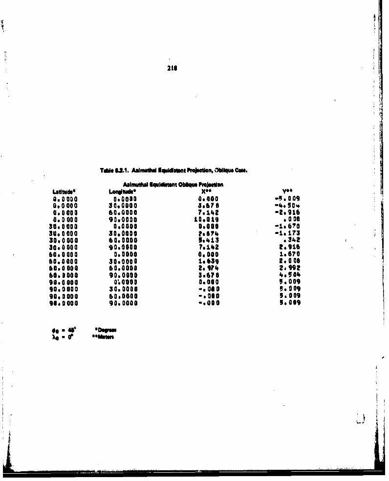
218

TW* U.I. Auimuthd Equliesnt P *auo n, Nbllqu Case.

Animutbe lUquldlut Oblique PimguilnLatituds* LOW&#l# ade.860000 0.0000 00000-.o040000 30.0000 Sob?$ -4*50'*0.0000 6000000 ?s.142 -2.9160.0000 9000008 10.019 600030.0000 0.,0000 0.000 -1.6703040000 M0O00 2*674 -1.17330.0000 60.0000 5.1413 .34230.0000 90.0000 ?o.142 2.91660.0000 040000 0.000 1.67060.0000 30.0000 19639 2.00060.0000 60.0000 2.9?'. 2,A99260.0000 90.000 3*6704S090.0000 0.0000s 0.300 9.0099000000000 MOMsoDI 5000990.0000 60000 000 w O 5600990.0000 90.0000 000 56009

219

In order to obtain the polar azlinuthal equidistant projection, let 00u 900 in (6.2.4),(6.2.5), and (6,2.6). We then have

*cor'l (Bin ~)(6.2.7) 1r

Cosn ~sin

uCos (f/2 O)

(6.2.8)

Substitute (6.2.8) into (6.2.5) and (6.2,6).

Cs0-sin (X - %0) Cos~coG sin (w/2 -)

-sin 0, -X0) (6.2.9)

sinG0 Co - O 5Cos (X x0)

sin (w/2 -)

-Cos (X - %'o) (6.2.10)

Equations (6.2.3), (6.2.7), (6.2.9) and (6.2. 10), with the inclusion of the scale factor,S, give the plotting equations used to develop a grid much as Figure 6,2.3. In this figure, allthe meridians are straight lines 0, true length, and the parallels are concentric circles, equallyspaced, The coordinates for the polar case are in Table 6.2.2.

The equatorial azimuthal equidistant projection Is obtained by substituting 00 I 00into (6.2.4) and (6.2.6).

Coe (CON 0Cos (X--X)J (6.2.11)

s8 s in 0 (6, 12)

The plotting equations are then obtained firom (6.2.3), (6.2.5). (6.2.11) and (6.2.12), withthe aid of the scale factor, S.

220

21i

0

Figure 6.2.3. Polar paimuthul equidistmnt projeution

221

TOM&=.22 Asmudhal Equldlitant Po*cUoi Paoar ~m.Asirnwthal Eqcuidstant Polar P.*c on

Latitude* Lonsitudo X**YO060000 0.0000 0.000 -1O.019060000 30.0000 5.009 -8067?0.0000 60,0000 8.6?' -5-00906000,0 90.0000 10.019 6 000

30.0000 0000011 0.000 -6.067930.0000 30.0002 3,34.0 -5.761.30.0000 60.0000 5.7,8 -3.34030.0000 90.0000 6.679 .00060.0000 0.0003 0.000 -3.34060.0000 30.0000 16670 -2.6926060000 60.0000 20812 -1.67060.0000 90.0000 30339 M,00090.0000 060000 0.000 -. 00090.0000 30,00Ga go00 a co90.0000 60.0000 -. 000 -0 CO90.0000 9000009 -0000 -. CO

00

WOh - 0911mrs

.................

222

6.3 Orthographic Projection 1201, 1221

The orthographic projection is yet another means of portraying the sphere upon theplane by a direct transformation. This is another projection that can be developed by apurely graphical means. In the orthographic projection, the perspective point is placed atinfinity. The projection rays fall perpendicularly upon the tangent mapping plane, afterintersecting the sphere, The geometry of this projection is shown in Figure 6.3.1 for theoblique case. Only a hemisphere or less can be portrayed on this projection.

Again, the auxiliary angle, 0, between CO and CP, and the auxiliary angle, 0, on themapping plane are needed. From the figure

OP' 0 as sin 0 (6,3.1)

x a OP' cos 6.3,2)

y OP' sinG J

Substitute (6.3,1) into (6.3.2)

x aS in cos } (6.3.3)t,;,:~ aS sin 0 sin #J

where a is the scale factor.

Equation (6.1.7) again gives

r s cos "1 (sin 00 sin 0 + coso0 coscos (X - e)) (6,3.4)

with sin @ readily available, since 0 < 4 < 90. From (6.1.6) and (6.1.8)

G taf[cos 0 sin ) -sin )0 cos 0 co (- ) (6.3.5)Lsin (X, - Xo) cos

Equations (6.3.3), (6.3.4), and (6.3.5) give the oblique orthographic projection.

The polar orthographic projection can be obtained from the oblique projection byletting Oo w 900 in (6,3.4) and (6.3.5).

0 w cos- (sin 0) (6.3.6)- cos (X - Xo) (

_ sin XO) J (63.7)

Equations (6.3.3), (6.3.6), and (6.3.7) yield a grid such as the one in Figure 6.3,2. Themeridians are straight lines, and the parallels are concentric circles. As the equator isapproached the parallel circles are compresed together, and distortion becomes extreme.The plotting coordinates are in Table 6.3. 1.

223

Figure 6.3.1. ometry of the ON1qe ocflo,Whle eetoe

224

P~g. ± ,rol.m PO paim*I

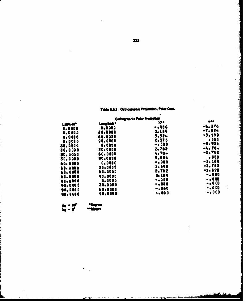
225

TeI. 031 . Onhnaphio PO s, Pe C.

LUmido Lae40*d X00

0.0000 0.000 we300 c6360.0000 MO3. 4189o000000 60.0030 9992' 43.1890.,000 90. 000 6,378 ,00o

30. 0,0000 -.000 5.32%300000 3000 2.76! -4.7630.0000 60.0000 4.764 -2.'623090000 9000000 g092 .0006004000 060010 =G000 -3*169

600000 30.0000 9lo$ -2076260.0000 60,0000 2.762 -109,60.0000 90.0000 39069 -.000

90.0000 000000 -O00 -, 00090.00000 30,0000 -.000 aOCO9060000 60.0000 ".0oo W.000908440 90.0000 -. 000 -000

**momu

ii*1

226

An equatorial orthographic projection Is liven by Figure 6.3.3. This type of projectionwas used to produce the first of the Lunar maps. The grid is obtained by letting 0o a 00 in(6.3.4) and (6.3.5). This is another limiting case of the oblique projection.

il -Cos ", [Cos 0Cos (X - Xo)] (6.3.8)

Sr ta tan' tn,] (6.3.9)

Equations (6.3.8) and (6.3.9) are then used with (6.3.3) to produce the required Op'd, In

the figure, the central meridian and the equator are the only straight lines. Notice, again,from the figure that distortion becomes extreme at the marlins of the map. Plottingcoordinates are in Table 6.3.2.

J.I '

is

227

Pilum, 623 Otwpe. sque"mial pmjuutos

tIon

22

I' IboIqu d I olag" MI Gmupqow Pf.m I*w cm.

C~d WP MGIOMBmI PNONton

O0O0 0$6000 .0o0 0000.0000 30,0000 3,69 D 0000040000 6000000 5o524 0.0000.0000 t0 0000 6,376 O.000

3000000 0,0000 .000 3010930.0000 $0o0000 to7 2 3.18930o0000 6000000 4,7il4 3,10930.0000 90o0000 5652'. 31696000000 00030 0000 5*9146000000 30o0000 tl*o9 1,l246000000 6000000 2.?62 So P.Oso0000 Oo 0000 30t85 1.92'.90,0000 060009 O000 6.3709000000 J090008 0000 60378900000 6000000 o000 Go,37690.0000 90.0000 0000 -0 376

sopseo " " *Dom

229

6.4 Simple, Conical Projetions 181, 1221

The simple conical projctions to be considered in this auction ane the one and twostandard parallel, and the perspective cases. AD of thene are basically graphical projections.

The geometry for the simple conical projection, with one standard parallel, Is dip.played in Figure 6.4. 1. The cone Is tangent to the sphere at the latitude 00, with centralmeridian at longitude ).This is displayed In section, with the cone tangent at point 0. Theconstant of the cone, from Section 1.6, is

0 cdsn 0O (6.4.1)

From the figure

PO a cot 00 (6.4.2)To obtain the spacing of the parallels, let the central meridian be divided truly. Thus,

with the help of (6.4.2)

P PO(* ) (6.4.3)

From (6,4.1)

ON CQ -)vj) (6.4.4)

Substitute (6.4.1) into (6.4.4).

0 (k- X) si Oo(6.4.5)

The absciss is, from (6,4,2) and (6.4.3)

x aSlcot 00 - (0 - 00)) sin IX - XO) sin 001 (6.4.6)

The ordinate is

Y Ws~cot 00 - [cot 00 -(0 -00 )1 cot~ I- ho) sin 00 ) (6.4.7)

where S Is the scale factor.

The grid for this projction is given in Figure 6.4.2 for~ 00 456 and h 0. AN ofthe meridians are straight lines, and the parallels are concentrc circles, equally weced. Thisgrid has frequently been used In atlases. Table 6.4.1 give the plotting coordinu~mL

The simple conical construction for the two standard parallels case follows fromFigure 6.4.3. The cone is defined to have true length standard parallels at #1 and 02. with#3 > 01 . From the equal spacing criterion along the central meridian

. . .. . ... .

2 230

00A

Plgws GAI. Ow o g o ol~ smW ii.. i mim gan wih a es Nhndod psind1N

231

Fipam UA2. Simple sone i welen, wtUh om I- t iu paradW

232

u.00U0 0.0O0s~o Qua 20096 4*

0aa4j 40.u 0 I*121, *I4e235

0.0000 .060 0 0 0, b*004 -3208Ih9664~o040 7o683 me2.0

060000 Tt.a1a000 9.%3226.7u.U000 90.00~0 0.204.s.2

a a0 0 9000400 -30340

1~0~ ~0040 t.789 -3&174%

150:0400 3.51.8 -2.881Selj4-1.879Lis0000 30.00 bo2 -.795

U0 0a0 0 6C000 6550%3

Su0000 9.00 .1 0040530*0000 - .oaoo 0.0 4.040SO

3060000 70.0000 2.430 t432

4000 9060000 4.303 1.S70

44000 4430 600Sc

306.600e36 291153.

8s0.00a0a0 7500000 $0029 3@54U60060 00000 ISM

11946046710 0

00 ) 3MO *74 S

4boODO 2*42 237?60*0000 2.190

233

A2 A'

Figure 6.4.. Gomstry far th Miimple sodullProjotionvith two standard parallels

234

PI .P 2 =a(02 0.1) (6.4)

From the similar trianglos in Figure 6.4.3

p1 a Cos 01

P~2 a COS 02

cob 01

Substitute (6.4.9) into (6.4.8). P ~

P1 a(2-1

COS 0

A radius vector to an arbitrary point P' of latitude 0 on the central meridian is, withthe requirement of equal spacing applied,

Substitute (6.4.10) into (6.4.11)

req ire en ofth cicl ofS 02 ( 0 )1 (6.4.12)

The next step Is to find a constant of the cone for this configuration. From the

requremnt f te crcl ofparallel to be true leatth at 01.

2va~~ cos 01o2flp

C1 W os0 (6.4.13)P1I

235

Substitute (6.4. 10) into (6.4.13)

a Cos0

C0S 02

Cosi 0050

02 01

We now have the equations (6.4.12) and (6.4.14) for a polar representution of the mappoint. The next stop Is to obtain the Cartesian plotting equations. Thea. are

C02-01x as

02-0

yma~o 02 i

X (I -Cvos I()X-% 0 )c 1 ) (6.4.16~)

Equations (6.4,14),O(64,1), and (6.4.15) yield the grid of Figure 6.4.4. Again, themeridians are straight lines, and the parallels are equally spaced concentric circles. Thisprojection has been used quite often for atlas maps whore it is not necessary to have eitherconfortnality or equal area. The plotting coordinates are in Table 6.4.1.

The geometry for the conical perspective projection is shown in Figure 6.4,5. The coneis tangent at latitude 00, and the central meridian has longitude X0

The constant of the cone, and the radius of the parallel circle of tangency are given by(6.4. 1) and (6,4.2), respectively. From the figure, the distance to an arbitrary latitude is

pop0 -atan(0-0o) (6.4.17)

We now have the polar coordinates for this projection. The Cartesian coordinates, using(6.4.1), (6.4.2), and (6.4.17) ire

236

Fiques RAA. Wn*W smill p,*odm with Io jgtnw" poulhls

r T AV tl'!

* 237

TAW. "J. Slems aomwedpk*ahm TWO- taddPmmh.

BImpe Cmmu TWO Sundmal Pv~bLottus'Lorit~ds* X* V.

15.0a QeSO0000, -to.070 4t 5 a0C 10a00 1:.742 -1.510

15.0,000 3.00000 3o426 11560000 46 0 a0 0 4o995 0426310 .60a0Do 606003,0 :.9882

30.0000o O.OV0000 .0030.,0000 1540,000 1.'438 .132t.,a 00 10000 2.828 6132330.0000 40iol 4.124 to.16110,0000 60*000P s .261 2, 02446-0000 aio I 0.000 Goo0 1.0704f.oQoo '16.0.000 1*134 1§77445.0000 30.00040 2. 230 of.083

400060.6000 4. 165 3o, 66600000e 0.0000 A.000 3o,3406040000 is 0.00 0 .:830 3.41660,10000 10*0000 1.633 3.64260.00000 '.5.00 2.381 ... 01060.10090 6040030 3o049 10715.10aco 0.00000 0,1000 5.0097500000 1560000 .1926 $s0ts?500000 30*0010 in 03S so20175.0000 .5.00300 L.509 164367SO0000 6000000 1.933 so.790

238

00I

Pkgw GAAL Ow-~ wo v Ij oo"pss i

239

* as [cot 0 - tan(**)

X (I -Cal (%-) sin ol) (6.4.19)

where 5 i the scale factor.

Equations (6.18) and (6.4.19) give the grid of Figure 6.4.6. The parallelq areconcentric circles, and the meridians are straight lines. The spacing of the parallels increasesIn either direction from the standard parallel. Thus, distortion Increases Significantly as onemoves north or south of the circle of tangency. This projection has been used for purelyillustratlvi atimes.

240

Pionr U4. PWngmsvs amu" p -1 Who

241

6.5 Polyconic Projection 111, 1251

H The polyconic projection Is a modified conical projection based on a variation of thesimple conical projection. The euence of the variation is that every parallel is a standardparallel, and there are an infinity of tanpnt cones.

First, it is necessary to derive the polar coordinates. The central meridian is true length,hand h l longitude X0 . Choose some latitude 0 as the extremity of the map, and the origin

of the coordinate system. Then, the distance along the meridian for a spherical earth isdm!I a(4 -*0) '(6,5,1)

From (1.6. 1), the radius to the point of tangency for an arbitrary latitude*, or thefirst polar coordinate, is

PM a cot (6..2)

and the constant of the cone is, from (1.6.4)

c u sine (6,,3)

The second polar coordinate is, from (6.5.3)

0 •(X, -Xo) sin (6.5.4)

The Cartesian mapping equations are

x ap sin 9

y d +p(I -cosO)}

Substituting (6.5.1), (6.5.2), and (6,5.4) into (6.5,5),

y aaS (0-0 0 (6.5.6)

+ cot 0 (1 - cos (X - o)) sin1

where S is the scale factor.

Figure 6.5. IIt the regular polyconic projection. The central meridian and the equatorare the only straight lines. All other meridians are curves. The central meridian, theequator and all parallels are true length. Thus, the distortion occurs in angles, areas, andmeridianal length for all meridians except for the central meridian. The polyconic projec-tion has beetn used quite often in atlas and road maps, and its wide acceptance has justifiedIts existence. A projection table for the polyconic projection is given in Table 6.5. 1.

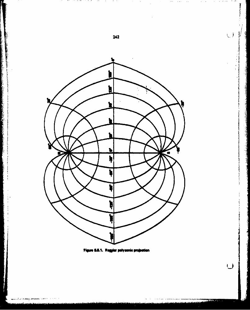
242 ~ F' ~x

j :3

4I -

II~; t I,

'It

-I2

I

P1gm SIl. Regi. plymnie pvujhalmn

U

Loom#* Xe. voo000001 0.000 00000 00000

00000 30.00030 36 dbo a 0000.0000 P600.00S 669 0. 000960000 9O0400 1040149 0.00000.00000 12006098 13#319 0.0000005000 101 0 16.690 0.0000'000000 MeOM*s 20*034 0.000

30&0000 0aa0a 0.000 3.34.030.0000 30.0000 20609 .0163060000 60.00050 6.51. .6130.0000 90.0000 7.612 0857938.10 13JL0.00 96867 0.66330.0000 15o000 140061 to.1163000000 1400000 1116017 L46 38760.0000 044010 00040 6679

6*0030.0010 1.613 ?0061tJ1.60 04002900 86.093

6090000 4960000 3.631 9.816040000 120.60019 3o.5?. lie theb0.0000 19000000 24629 it.712460.0000 180.0000 is.lei$ t1.7139000000 000040 00000 100 t90.0000 30.0000 0001 1090119840000 9000000 -000 10. 01990.0000 '4060000 MO00 10.019900300 120.000ft Gas000 10.0199040010 190.0000 -OO0 180.01990.600040 1A0.0000 .000 100 19

es ocmv #*n MuN

244

The transVers POlyconc CiAN follow$ from applying the rotation formulas of Section2. 10 to the plotting equations for the regular case. Write (6.5.6) as

x = S cot hsin (a - *0 sin h)

ymaS (h-ho(65)

+ both [I -OB [(a - 0)sn h1])

where h, , a, and asar measured in the auxiliary coordinate Aystem, and S is the scaleIfotor.

The rotation formulas, from (2.10.4), (2. 10.,5), and (2.10.6)o for the transverse case,with 0, are

sh .Cos 0COB (X- N)

cos a cos h *sine 658

tan si*.n (X~-?~ cot* JEquations (6.5.7) and (6.5.8) are used to deriv, grids such as the one in Figure 6.512

The transverse polyconic projection has also enjoyed wide acceptance in atlas and roadmaps.

Air

245

6.6 Simple Cylindrical Projections 1221

Two simple cylindrical projections will be considered, These are the perspective andthe Miller, In both cans, the sphere is transformed to the intermediate developable surface,the cylinder.

The perspective projection is a graphical representation.

Figure 6.6.1 shows the grid of the cylindrical perspective projection. The abscissa ofthe plotting equations is simply

x aS(,- )0) (6.6.1)

where s iN the scale factor, and 4 is the longitude of the central meridian. The ordinatefollows from consideration of the figure

y aStan (6.6.2)

Then, (6,6.1) and (6-6.2) are evaluated to obtain the grid, Distortion becomes veryreat as higher latitudes are reached. Thus, this projection has served In the role of an

illustration.

The Miller projection cabs for the equator to be 4a in length, and the meridian to be wsin length, Thus, the meridians am true, but the equator is compressed. The total area ofthe map Is 402, which is, by design, equal to the total area of the sphere. The plottingequations are simply

x-2 (X ()-%0)

(6.6.3)

where X0 Is the longitude of the central meridian, and X. NO, and # are in radians. Again, SIs the scale factor.

The Mid resulting from (6.6.3)1 Is shown in FIgure 6.6.2. In general It Is better to con.sider this projection as conventional rather than equal area. The distortion at middlelatitudes is less than In the equal area cylindrical, but it is greater at the equator. A plottingtable Is included as Table 6.6, 1.

246

------ - -

------ - -

- - - i ~ - A

~ mm - - mm -

mm - - - - -

~ - - - - mmm

- - - -

- mm - - - - -

- - - mm~ - - mm -

- -- -

mm - .mmm~. - - -

- --- - a -- -

PIpi. 6.6.1. P.ups.~v. oyIIndvIuI ~JutionIi

,, I,,,'

247

I

b _ h _- U

p- - m

- - - - V-

- U- ~ U-. -

- U- - -

- U-

U- U- U- U- ~

- U- ~ - U- -

- -- ---

U- - - U- U-

U- - ~- -- - *1 -

U- - U- mI ~Piguig 66.2. MIIIgr gylindulul p.ojmtlon

A

II

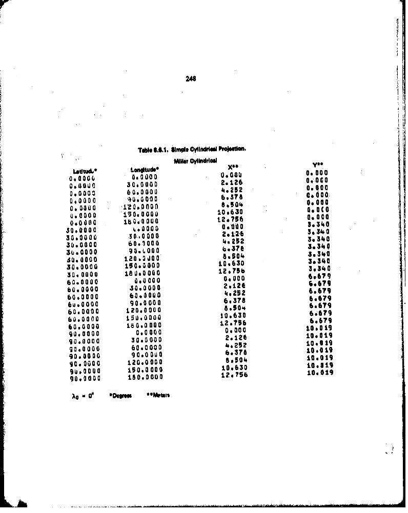
248N

Table 0... UImple Cyllndries Pvoojnf.

Millet OyllndrledLsaltu& Lanltde*

o.0oo0.0000000 000000.04O30000261,26 0t..00

0.0000 ±20.0000 oo50 000

0*0000 A O.0 0 1063 0.C000O 0.00 1.5 00000

30,000 0 At Q0OO30.0000 30-10000 2 s.2b2 3.340

30000 60.1000 4*272 U.340

30.0000 90.i4O00* 8.504134

30.0000 to 0.000 a10,630 3.3140

30s.0000 180.0000 12 s?5b 393140

6000000 00a0 00000 07

60.000 30.0002.126 6.679

b0.000O0.00 49.252 6.679

6u00 00 90.0000 60376 6.679

60.0000 120.0000 8650~4 60679

60.0000 150.0000 10.630 6.679

60.0000 18000000 ±2.756 60*679900000 OGOODDOUG10.019

90.0000 30.0000 2.12e 100019

9000000 60.0000 4.252 1,1

9060000 90.0090 60378 10.019

90.0000 120.0000 665014 10.019

9u.0000 150.0000 10.630 10.319

90.0000 180.0000 12.756 10.019

AO 0 *Drm "Wten

249

6.7 Plate Curre6

The Plate Carr6e is a simple cylindrical projection with the equator as the standardparallel defined by a simple mathematical rule.

The meridians are true length straight lines, parallel to each other. The meridians aredivided as on the sphere, so the parallels are their true distance apart. The parallels and theequator are also straight lines, perpendicular to the meridians. The equator is also dividedas on the sphere.

The result of this Is the square gid of Figure 6.7. 1. The plotting equations which

produce this rid are

x a aS(%,- Xo) (6.7,1)

y a aso

where X0 is the longitude of the central meridian and S is the scale factor, The angles 0and 0 are in radians.

The distortion in length is extreme along the parallels, The poles, which are points inreality, arc represented as straight lines. The projection pretends at neither conformality norequivalence of area. It does serve as a reasonable diagrammatric representation of data, andis found in many technical reports where no greater cartographic sophistication is required,The Plate carr6e is a map done on standard graph paper.

30"

-l80 -5 0 - - -- - -- W -

230

-6.7.1. Iste o-rra proataon40

,, , i ,-.. - - a ....... i'- -......i - --' .. ~

250

6.8 Carte Pamtllelogrammatlque

The carte parallelogrammatique, or die reckteckise plattkarte, has a fancy name for asimple projection. It is essentially a variation for the plate carr6e, In which two standardparallels, equally spaced around the equator, are taken as true length. The meridians orealso true length. The plotting equations, In which 0( is the latitude of the standard parallels,and X0 is the longitude of the central meridian, are,

x s coo 00'(W - %0)(681y- aS

in which 0, X, and X?. are in radians, and S Is the scale factor.

.A grid developed from (.6.8.1) is given In Figure 6.8.1. This projction has seen somelimited use in atlases. -It was developed as a means of reducing some of the distortioninherent in the plate carr6e. The area between the standard parallels Is smaller 'and thatpoleward from each standard parallel is larger than on the earth.

- -3

0

Figure Car1 Ote panuIeuoauarmueique projeslon

251

6.9 Globular Projection 181, 122)

Thv globular projection Is a convential means of portraying a hemisphere within acircle. In this projection, the central mieridian, With longitude X.0, and one halt of theequator are disaters of the circle. The central meridian and the equtof ore 'divided truly.

Define a typical cirals of parallel of latitude,, ThWis shown in Fillgut 6.9.1. Let dbe the distance tram the'equator to'the specified latitude tlonguthe central meridian. Let cbe the chord length, and h be tha distance from the circular arc to the chordo Lat p be thepolar radius vector.

the distance along the central meridian, between the equator, and 'the circle of latitude

dwROa (6,.1)

From the figure

c U24 Cos (619.2)

hwa sin 0- aO (6,9.3)

From the geometry of the circular segment

c 0 %4-h~- h)(6.9.4)

Substitute (6.9.2), and (6.9.3) into (6.9.4), and re-arrange, to obtain the first polar coordi-

nate, p.

C- 4h(2p -h)

2p -h *

2p I h +

.1 -FaGi. -0 442 C082 12 ~4u (sin-)J

sil 0 + JOS (6.9.5)

The sveond polar coordinate, 0, follows from the Seometry of the circular segment,also.

252

d

Pimw, GAI. Gusmb v l do WP - p mie eln

253

Substitute (6.9.2) and (6.9.3) Into (6.9.6)

0 2tan-, 2a cos 0a(sin*

*2 tan- (6.9.7)Lain 0-O

The parallels are divided equally, Thus, a second auxiliar angle /ican be defined bythe projection

Substitute (6,9.8) into (6.9.7).

2(k Xo)tan(6.9.9)W~Q ' \sin 01

The cartesian plotting equations are

sin ~(6.9.10)

Substitute (6.9.1), (6.9.5) and (6.9.9) into (6.9. 10).

m.jAW sino~-O

X siI( )tn 2 cos S(6..11

xl Co 2[ X))tal- cs (6.9,12)

where S is the scale factor,

254 .)

Equations (6.9.11) and (6.9.12) produced the pid in Figure 6.9.2. The globular projecmtion has been used for atla maps.

so]OrI

-W r w w

P1W.w~w~. u upAi

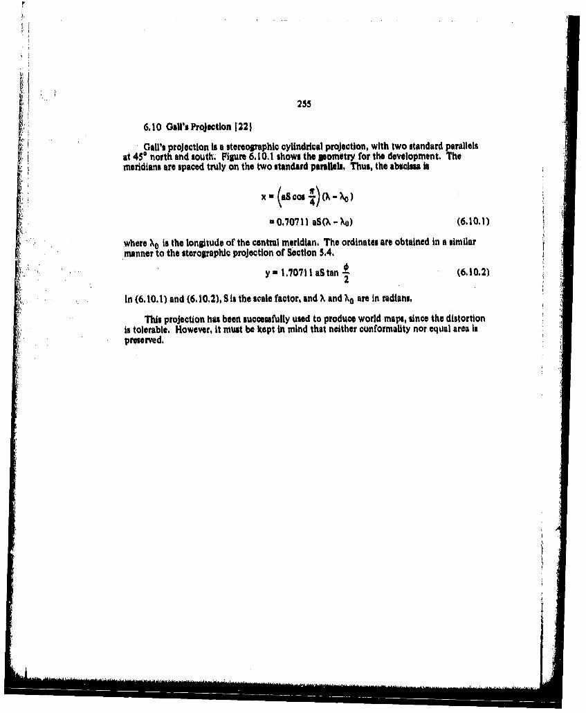
255

6.10 Gall's Projection 1221

Gall's projection is a stereographic cylindrical projection, with two standard parallelsat 4SO north and south. Figure 6. 10.1 shows the pometry for the development. Themeridians are spaced truly on the two standard parallels. Thus, the absoiss is

xa(aScg (-

*O,70711 aS0,-Xo) (6.10.1)

where kn Is the longitude of the central meridian. The ordinates are obtained In a similar

y a 1.70711 aS tan 2 (6,10.2)

In (6. 10. 1) and (6,10.2), Sis the scale factor, and X and ho are in radians.

This projection has been successfully used to produce world maps, since the distortionis tolerable. However, it must be kept in mind that neither conformality nor equal area ispreserved,

256

.4f

Rpm o~l.(Wlpi olso

257

6.11 Van dor Gifnten Projection 1221

The Van der Gtinten projection contains the complete sphere within a crble. Thisprojection has seen some use in atlas and National Geographic Society maps, While it doesnot pretend to display conformality or equal area, it does present a pleasing representationof the earth's surface. There is neither the east west extension in higher latitudes that ischaracteristic of the Mercator, nor the extreme compression in these areas, as shown in thesinusoldal or Mollwoido.

Figure 6.1 1. Ives the geometry of the projection. The equator is divided equally,and is represented by the line VQ. The line NS is the central meridian, which Is also dividedequally.

Consider a purely graphical construction of this projection. Join N and V. Locate anarbitrary latitude A' on NO, where

OA' NO w/2

',2NO (6.11.)

Draw AA' parallel to VQ. The Intersection of AA' with NV is B. Join 9 and Q. The inter-section of BQ and NO defines the point C'. Draw CC' parallel to VQ. Point C constitutes,one of the necessary points of the projection. Its symmetric Image about NO is a secondsuch point. C" connect A and Q. AQ Intersects NO at D. This is the third point necessaryto completely define a circle of parallel.

A circular arc, whose radius Is uniquely defined by the location of points C, D, and C",is drawn to obtain a circle of parallel.

Meridians are also circular arcs. These are fit through the poles and the equatorialpoint for the particul~r longitude. From the central meridian, of longitude X0, the point onthe equator is

d-VO (6.11.2)

The usual means of constructing a map using this projection is to inscribe the grid, andthen plot points on this grid as functions of and X.

LW

258

PipmO .11.1. Van der Galntmn'spasujaon

.. .............

259

6.12 Murdoch's Projection 1221

Murdoch's projection has been used in atlases, It is a secant projection, but differsfrom the simple conic with two standard parallels. There are three variations of this projec-tion, but only one of these variations will be derived from Figure 6.12. 1.

In the first variation, the parallels are spaced their true distance apart on the centralmeridian, with longitude 0, The constant of the cone is

/1 + 2c in 2(612,1)

where 01 is the lower standard parallel, and 02 Is the upper standard parallel.

From the conditions of equal spacing

2sin( 02-0CB a j (6.122)

The middle latitude is01 + 03;

- a (6,12,3)

The radius of the middle parallel is

TB CB cot i (6,12.4)

The radius of the lower standard parallel Is

PI *TB +( -0 1 ) (6.12.5)

Thus, the first polar coordinate is

p =p - a( -01) (6.12.6)

Substitute (6.12.2), (6.12.3), (6,12,4), and (6,12.5) into (6,12,6),

102 -01~s in 01 02

P { 8 2-*t cot 0) (6.12.7)02 01

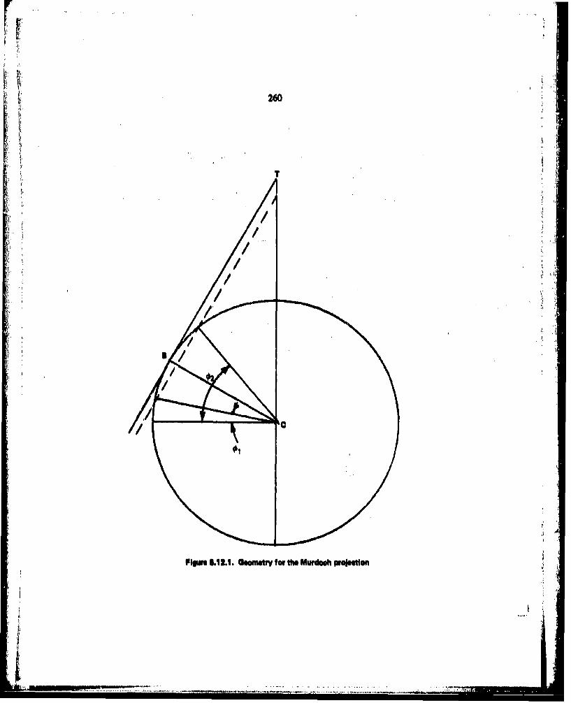
260

T

Pion M2.1. Geowetr for the Murdoebp.l o

261

The second polar coordinate is

0 =(-o)C (6.12.8)

Substitute (6.12.1) Into (6.1 2.8).

0- (h - o)sin ( / (6.12.9)

The cartesian plotting coordinates are

x= wp sin 01S(6,12,10)

y" (PI -p0 - Cos 0)]S

Equations (6,12.), (6,12.7), (6.12,9) and (6,12, 10) product the desired grid, where Sis the scale factor,

L . ...... ....-- .-." . .. .... -i- ..... .......... .. .. ...-"...T T '

r

262

[l 6.13 Stereograpbic Variations 1221

Several variations of the stereographic projection have been developed to reducedistortion in regions of particular interest, These are the James, the La Hire, and the Clarke.All of these ate geometric perspective projections, and can easily be obtained by an altera-tion of the stereographic projection of the sphere. Figure 6.13.1 shows the location of theprojection points for a polar projections of these variations as compared to those of thegnornonlc and the stereographic. La Hire took the projection point as 1.71 times the

* radius of the earth, James used 1,367 times the radius, and Clarke's value varied between1.35 and 1.65 times the radius. We will consider a derivation of the plottig equations fora polar projection.

From Figure 6.13.2,

tan -a(l + c')

p = a(l + c') tan , (6.13.1)

It Is now necessary to relate and 0.

AB a sin (90* - 0)

t a cos A (6,13.2)

an I • Cos (900 - 0) + c'}

AB (6.133)

a (sin 0+ c')

Substitute (6,13.2) into (6,13.3)

t a costan = a(sin 0 + c')

sin + c ' (,34)

Substitute (. 13.4) into (6.13.1).

a + C') cosP= Bil +6, 13.5); sil q) + L

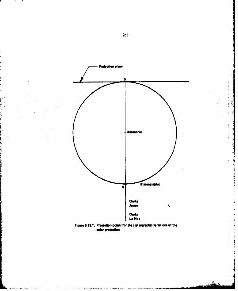
263

Projection pliane

N

Gnomonic

Corks

James

Clarke

La Hire

Figure 6.13.1. Projection points for the seteogrephic vegritiom of thepolar projection

264

FIir 6.1i;2. Geomatr for the steorepgapil va#Itne

isj

- 265

The Cartesian plotting equations follow from (6.13.S)

sin a(+c's o~-~

XSO +') Cotosn,-

where Sis thesale factor, and chis Siven by Table 6.13. 1.

This series of projections has had some utility in geodetic mapping.

Table 6.13.1. Values ef e'for t Urnwetwo of fi.

Name G

Clarke I.*6Jam"s 1.367Clarki 1.66La H Ire 1.1,

. ... .....

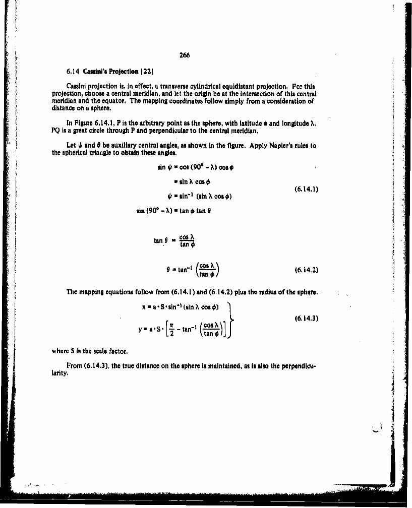
266

6.14 Cassini's Projection 1221

Cassini projection is, in effect, a transverse cylindrical equidistant projection. For thisprojection, choose a central meridian, and let the origin be at the intersection of this centralmeridian and the equator. The mapping coordinates follow simply from a consideration ofdistance on a sphere.

In Figure 6.14.1, P is the arbitrary point as the sphere, with latitude 0 and longitude X.PQ is a great circle through P and perpendicular to the central meridian.

Let 0 and 0 be auxiliary central angles, as shown in the figure, Apply Napier's rules tothe spherical triangle to obtain these angles.

sin 0 a Cos (90* - X) Cos €,-sin X cos os

(6.14.1)=sin " (ain X cot 0)

sin (90* - X) a tan tan 0

tan 0 - -tan

09 tan"1 (Cos X (6.14-2)tan 0-

The mapping equations follow from (6.14.1) and (6.14.2) plus the radius of the sphere.

x a S sin "1 (sin X cosO)

(6.14.3)YN rS 1-a-I lcos "

where S is the scale factor.From (6.14.3). the true distance on the sphere is maintained, as is also the perpendicu-

larity.

I:

i ~~ ........ I.II.I.

267

Pp.6.14.1. Geomety fw do CIpejellA

Chapter 7

THEORY OF DISTORTIONS

Distortion Is the cartographic bane, This was mentioned in Chapter 1. No matter whattechnique or algorithm Is used, distortion will occur in length, angle or area, or in a combi-nation of these. Throughout Chapters 4, 5, and 6, it was pointed out where distortions dooccur for particular projection, but this was treated only qualitatively, This brief chapterwill deal with the general theory of distortion in maps in a quantitative way. Formulas willbe developed to quantify the distortions in length, angle, and area. Then, these generalitieswill be applied to the most frequently used equal area, conformal, and conventional projec.tions,. Thus, we will have suggested a numerical means of assessing the acceptability of amap for a particular application, Finally, some of the different classes of maps will be com-pared In a qualitative manner.

71 Distortion in Length 1101. 1201

In order to describe distortion in length, we will consider a two dimensional plottingsurface, and derive terms for distortion along the parallels and meridians, as compared totrue distance along a sphere or spheroid, The derivation begins with the first fundamentalforms of the earth and the plotting surface, The ratio of these fundamental forms Is definedto be m, From (2.3.3)

n2 * E(do)2 + 2 Fdo dX + G(dX)2 (7,11)

e(dO)2 + 2 f do dX + g(dX)2

where the capital letters refer to the mapping surface, and the lower case, to the sphere orspheroid. Since we are dealing exclusively in orthogonal systems for the mapping surfateand the earth, the substitution of F m fa 0 into (7, 1. 1) yields

m2 a E(dO)2 + G(d )2 (7.1.2)e(do)2 + g(dX)2

The distortion along the parametric 0-curve, or meridian, where dX 0 0, is, from (7,1.2).

mm - (7,1,3)

und the distortion along the parametric X-curve, perpendicular to the meridian, where do •0.13

268

*1

269

InP (7.1.4)

These distortion. in distance will be applied to particular projections in Sections 7.4,

7.S. aidd 7.6. True length corresponds to m. mm M 1.

7.2 Distortions In angles I10 1, (201

Figure 7.2,.1 a is needed for the derivation of the angular distortion, Again, from thefirst fundamental for the model of the earth

(d$)2 we(dO)2 + 2f do d + 8(dA)2. (7.2.1)

The angle between the parametric -,and A-.curves intersecting at point P is

+ (7.2.2)

Consider the differential parallelogram to be sufficiently small in area, so that It can betreated as a plane. Then, the law of cosines applies.

(ds)2 *e(do)2 + g(dX.)2

+ 2 veeSd dcooAw (7.2.3)

Equating (7,2.1) and (7,2,3)

Also,

sin w *(7.2.S)

Since we will deal with orthogonal systems. r. 0, and from (7.2.4) and (7.2,5)

Cosw W 0show *I

Thus, from (7.2.2)

a + W /2 (7.2.6)

.~~' .. ~, .. .. ..

270

a)* Earth

A

AA

271

From the figure

Cos a %/- dl

dXsi g (7.2.7)

Consider now, Figure 7.2. 1b. where an infinitesimal part of the projection surface isshown at point V, orresponding to point P on the earth. From the figure, for the orthog-onal mapping surface,

coo A-~'

si A (7.2.8)

Expand

sin (A - a) in A co aot

- cos A sin a (7.2.9)

Substitute (7.2.7) and (7.2.8) Into (7.2.9).

sin (A -a) ,%;a Xd VS

- NCO- - vT, d (7.2.10)

Substitute (7.1 .3) and (7.1.4) into (7.2.10).

sin (A -a) u (mi -m tr) d~ dX~(..1

In a similar expansion,

sin(A +a) (mp +mm) d d (7.2.12)

Re-arrange (7.2,11) and (7.2.12), and equate

sin (A - a) M sin (A + a) (7.2.13)Mp + nim

272

Equation (7.2.13) is another transcendental heast, For a constant mp and mm it canbe solved by the Newton-Raphaon method. [141 Write (7.2.13) as

f(a) 0

*~~M sinAt (A + am)min (A m- cI(- MR (7.2.14)

The derivatdve'of (7.2.14)1.s

*Cos (A- a) - 0 o (A - a) (7.2.15)

The Newton-Raphson scheme for the solution of (7.13)1is then

f* An (7.2.16)

UU

sin (An a - ni mm ) sin (An + a) (..

coo (An -a) -( m m ) coos(An +a)

As an Initialization, let A0 a. This iteration Is rapidly convergent, and easily computerized.

This technique will be applied to the equal anea, and the conventional projections. Aswill be seen in Section 7.6, (7.2.13) has a unique solution for conformal projection.

7.3 Distortion in Area 1101, 1201

The are& on the map is, from (2.3.13)

Am fE 2(7.3.1)

and the area on the model of the earth Is

A / 2-- (7.3.2)

The distortion of ares, is hereby defined to be

273

DA - Am/A.

=E -F (7.3.3)V e_-fl

Since the systems are orthogonal, F = f a 0 can be substituted into (7.3,3),DA = .__ (7.3.4)

V e3

Substitute (7.1,3) and (1,4) into (7.3.4),

DA " mp mm (7.3.5)

Now we are in a position to consider these distortions in terms of selected projections,In what follows, the distortions will be derived for polar and regular cases. They applyequally for the oblique, transverse, and equatorial cases. The only difference is that a issubstituted for X, and h Is substituted fore,

7,4 Distortion in Equal Area Projections 1201

Equal area projections, by their definition, have no distortion in area in the mapping

transformation, Thus, ftom (7.3.5)

DA mp mm

(7.4,1)

It is seen from (7.4, 1 ) that mp and mm are the reciprocals of each other. We will now con.sider the more important equal area projections of Chapter 4, the Albers conical, theLambert polar azimuthal, and the cylindrical, The distortions in length and angle, at anarbitrary point, will be derived. In the case of distortions in length, only one of the dis-tortion factors need, to be derived. Equation (7.4, 1) is then used to find the seond one.Thus, in all cases, the easier of the two will be chosen for the derivation, and the secondwill be its reciprocal, All cases will be derived by considering the authalic sphere of Section4.1.

Consider first the conical projcction with one standard parallel, the first of the Albersprojections, From (7,1.3), (4.2.1), (4,21), and (4.2,5)

mm"

'2

274

Rc os (7.4.2)

Substitute (4.2.15) and (4.2.19) into (7,4,2).

sino 00 /1 + sin 2 0o - 2sin* sin 00

R coo s

, pirl 0n o- 2 siln 0.sin 0o" COS *s (7.4.3)Cos,

From (7,4, )

mp Col (7"'4,,

I + sin2 0 - 2 sin, cos ;0'

It is obvious from (74.3) and (7,4.4) that an expansion in scale in one direction is offset bya contraction in the direction orthogonal to It,

Consider next the case of the two standard parallel Albers projection. From (4,2.6),(4.2.32) and (7.4.2)

MM (si n1 +sin02) 2 + 02 (sin 2 - sin (74.)2R cos / 2 sin 0 +sin 2

From (4.2.33)

(sin 01 + sin 2) /4R2 cos2 +4R2 (sin 02 - sin 0)mm 2R Cos 0 Vsin 01 +sin 02

+ (sin 01 + sin02) (sin.02 - sin 0) ('7.4.6)coa,

Then, from (7.4.1)

mp n / cO. 2 . (7,4.7)m os2 0+(sin'1+ sin 2 )(sin*02 - sinO)

Nuxt, we shall consider the polar azimuthal, or Lambert, prujection. In this CUse,sin 00 1, is substituted Into (7.4.2)

M n (7.4.8)

275

Substitute (4.3.2) into (7,4.8)=RJ :2 '(1 - -sin

K com 0 ..

V (/2I - sin ) (7.4.9)cos ,

From (7,4,1)

0 I (7.4.10)

The cylindrical equal area projection was treated In Section 4,5. From (7,1,3),(4.5.2), and an application of the fundamenthl transformation matrix

-e

VR 2 cos2

L (7.4,.11)

From (74 )

mo a cos (7,4.12)

Note that the four sets of distortion factors, (7,4,3) and (7.4.4), (7.4,6) and (7,4,7),(7,4.9) and (7,4,10), and (74,I 1) and (7.4.12) are all independent of longitude. Thus, inthese cases, distortion in length if a function of latitude alone.

In order to find distortion in angles, substitute (7.4,1) Into (7.2.13).

sin (A - t) " sin (A -a)

ling2- I\sin ( A - 0)al I __ si n ( A + ,a) (7.4.13 )

Equation (7,4.13) can now be solved for constant mn by the Iteration method of Section7,2,

*1 -- U

276

Frm'hapter 5, It is recalied that conformal projections are characterized by the

7ac 5 t stotoinC frmlroetos11

for an orthogonal system. Thus, from (7, 1 3) and (7.1 .4), at eyery point

This rI.lationship makes the work involvmd inI any derivation of linear distortions ealsier,

since only one ratio or thle first fundamlenltal qlUantities nee~ds to IV evalted. III tis sec-

tion. the piolar stercograplik, the Lanmhert con formal with one and two standard parallels,

anld thlt Mercator projection will be considered, These distortions will he based onl thespheroid as thv earth surfau.

[or the Lambert conformal projection with one standard parallel. 1,181ing (7,1.4)

(7.5,3)

Substitute (5,.2) and (5,.3). arnd apply the fundamental transformaution niatfix to2

pC )

=R 1 Cos~ (7.5.4)

Substitute (5.14) andI (5,3,21) into (7.5.4).

iii~+ o t

x (1 4i 0 i

-Q esill

{ t ............ ............. .l (. ..s. . .

277

For the two standard parallul case, the distortion inI length Is obtained In a mannersimilar to thle one standard parallel ease. F'romi (7,5.4)

~~ (7.5.6i)

Fkiuatlon ( 7.5,6) is then evultutted with the aid of' (5. .28), (5.3.3 1) and (5,.332).

[ror the stereographic polur projection, the litieur distortion along the puramectriccurves may he found by considering t!!(. plane and the spherold. Fromi the polar Coordinatesof' the mnapping 1111111

G p.

I or the spheroid,qauinl

g = oS2 (7.5.8)

Substituting (7,5.7) bind (7 .S) Into (7.5.1)

SubStitutC (5.4,() into (7.5.9) m 1 o~(,,)

ii tanl

v Qlei~ 2 + 7..0

Asa 11in1l CI(tor-t InI this Sectloii, We Will conISidci theQ regullr Mercator pr(oiection,Agatin, the spheri 1haS the first I'l iliIIenttil I Lquan1tity

g = ~ Cosi 7.1

Vol. (le plotting surlacc

U a a2 (.,

SutbIs tt iut v(7,-1.) 11 nd (,5.) 1) 1nto (7. 5,1)

O.S 0RI) Co 0rJ(,,3

278

Cosider thle linear distortions giiven inl (7.5.5), (7,5,6). (7.5. 10), and (7.,13). Again,All 01' these eqautiolls (lependI only onl latitude. In tiny practial evalluatiOnl 0l' the.si dis-tortionls, it Is suil'Ticion t to treat thle 0,11-111 as a sphere, rather than as a spheroid, This is dom,by letting V =(0 ill the ~qluatilils It0t tile distor-tiIll Th eqItiitions9 then1 reudUce to easil1y

For the distortion Inl anlgle at a pohint, substitute (7,S.2) into (7.2,13) *sil(A - a) slA a

A (V (().

A ='(7-1.14)

[ha k, , atithe properties oI' the coil formlalI projCtion is that angles 111-e preser-ved In thle

tranlst'ornliaionl

7.6 D~istortions Iii Conventional ProJections IllI.1I1201

it ticeIlie most im portll t Conven I11 llanI rjectionlS Will be conlsiderQd, These arethe aon~~tic (le a~'nt~t ha -qilal, aind thle polyconic. In these pro ections,

Ill 4, 11MI ndt itl - illi Since I here ex ists nio sim iple relatlion betweenl the two dis.tort ils ill lvigc i'l h parametric cuimes, I snecessary to solve tor btIlowever,basic dbiiosmake thssimple in many eases.

C'onsider lrxt thle polar glilnotlic ptqoektioil, liom th10 geom1try Ohf 1the Vase Filie:

R tahn 6i dXR sinl 6

II

For the distortionl pe1i'ldicili' to thle meridian

till)~(7,2

true r tyhe liioI1,0n.1 l ii 111 pola projection, the distance aloing the menld nns Is

Trhe dIsta nec along tilt parallels Oil the. 1111p, lis Comp ared to those Oil tilt sphiere follows friomthle g~eometry of' a circular segment,

Z2 i7/2 -

TIhe lust pro ectil to he consideredf Is the regular polymcnic. Bly the ussum pt ions Ii.

ip celuded Ii the durivtli of the projection

The d istortioni along the mnerli ans is, withou)Lt pron t, gjVven by

II + C~*LoS.2 N~Ii e6

lor thle giloinloiic uind LIV.ilItIlial Veclildistaltl pi'IectloI01S, the linear diStolrtion isindepenldenlt of' lonlgitude,. lowevei, the distortion Ill thle meridian lakne Iom thle polyconileks 0 I'nCtln Or both htititudeI anld lonlgitudeIC

D~istortion Ill angles at it point in aISt be1 iawid by the numerILicIa l tie 0i'0(72,17).

7.7 Qtnilitn five Comparisons 19 , .1221I

While a nulltialvil approach Is certa11Y inl ui(Il liative comparisons of' the variusprojections tirc also usvrtltd This svet on will corn pare suelecd liiIiIIIat hl world, Cylinadrical,and colii l proictilils.

IFigLIr 7,7.1 compures five of' the liinatll polmr projections: thle equal areau thleequidistant, the artho~graphic, the stereographic, and thle gnomonic. Begin ning with tileIart hiogra 1hi C. there is at teady graldationl or parallel spaicing. endling With lthe gliollillic.The ortihograpic projection so lI'er distortion Lis the equautor is aipproachled, The parallelsONc unequa11.1lly S111ce1.l Mnd tireC bunched together~l Close to tile equalltor, The convergencee Of *

thle parallels is not as sever ir]' theV eq111ua l rea 10 proectio, rue eq allistilant pr1o-ject Ion halsequally Spiaced partil Ics 1s,The ste rogra i ic anld gnuaio oik projec tions I mav at diverge e Otfthe Concentric parallels ats thle equator Is approachled. The distori'ton In thle gnlonlonlic laice -thoul Is more severe, and tile equaltor itself' Canl ne0vr he port rallyed.

280

Storeographic 0 ~ 311 3 60' Gnomonic

Orthographic

Figure 7,71. Comparison of azimuthal projections

............. iN

281

In FigUroe 7,7.2. One quaI'drant of' thre equal area world maps of' the same scale isplotted. mhe sinusoi provection results in at pointed figure. Hlowever, the Mollweidc Is a Ismooth curve, The parabolic projection is in hetwieen the two in terms of' distortion, Notealso, there is ai variation in the spacing of the parallels.

InI Figure 7.7.3 Is at comparison of the Mercator, the Plate Cursh, -and thle cylindricalequafll area. The Plteo Car~e has equal spacing along the meridian, The spacinig for the

Mercator increases ats higher latitudes tire reached, This Is reversed in the equal areai cylin-ciricul. Hlere, the spacing decreases ait higher latitudes.

Three conicail projections of' one standard parallel are compared In Figure 7,7A4 1These tire the equal area, the perspective, and the Larnbvrt conformal. In the equal areaprojection, the parallel9 aire closer Lit higher latitudes, and farther at lower latitude. In theLambert conl'ormai, the spacing diverges north and 80outh of the standard parallel, hut inI agradual way, InI the perspective projection, the divergence Is for more severe.

!i .

i~i ",32

I I'

// / Ii

Ii/ l ii

'1' II

/1I I

'I / "1 iiIt / 'I

I" II

i lhlP~ure 7,7,2, Compalsofi of equall IOTe I world ma, .

L. 2 .I

283

.33

Fiur 7,._Cm aiofcyidia rjcin

AI

.........

294

yo1

LLu

illsreor 111 Lt er t I) CONCLUSIONI

Thisreprt lli utellple tobring togvee inl ColC (locullil t a fair-ly coinpleI etS of'mapl projection ecluttions. To this eld, it wais necessury to define the problem. Lind to intro-duce the terminology of' mapping. Then, the basic tranisformattions of' mapping were dle'rived, The model of' thle earthi, with the current valuecs ol' Its parameters were then needed.Next, the three classs of map proIlcetions: equall area. Coilforml 1. aind convenltional, wereConsidered 0one by one0, F or Vault class. it nuimiber of' projeoction Schemes were investigulted,F~inailly, at moi)11 ofmnmrically vailuating distortion was given. Thlis has beenI anl introduc-tion to the theory of map projections.

l-iowCvve. of liii more utility to the uisers or mis is thle priletice oft, mtip pro~ectionh.Tihus, inl almost Lill eases, thle final1 result Is expreQsSed inlana cillWirtei ma~pping voordi-mites. The form a ilas t'or thle most5 uIseful or' these pioiect lols wervemiibedded Iiii LI orn palerprogiain , anld it vane I y of' plotting t11b11S were gene0rated,

TIhe level of, ma1 thle ilatie's cosenl ror thle (Ieriva t lonls was5 consistent Wil lith (VStrictIntention of obtaininog usable cartesialn plotting equailltionis. Previous paiicuails hlave 4ti '-fered from one or thle other of' two Opposite ex trenivs, Manly presenit thle pro ect ionl Withlittle or nio derivation, aind In tend to hollow min~lly La graphicail Lipproich. Inl these, thleSpheroid Is not considered. The opposite aipproach Is one of' nititthinatical elegince. The%milk( durivailionl Is followed inl It nunmher of' wys thatI suem to thrive onl complexity. Inlthiis report, thle ckAlCept.S of1 dl ftereutiaL geomotry Were Iim posed as the an ify ing principles,Ill mlost ow."s. 11lie derivations WeOe reltively Clean1 111l straighit-forward. Ill soic oitherccosvs, such its t lie Pa~rabol iv projection, It was nveessairy i() use it uiniq ue method. Still, the

derivultioiis reillilned uitilitarianl,

datta pinlts f'or thle gra I icules which appeari as figures Inl (ha ptors 4,5, Mind () Secon1d, t hoSeplotting I ablvs which ar: generii I. andi depenid onI no Staindard pit ial d. cll he lised to prloducLea uslible grill for Liny applicatilon.,T tIi ser chin choose Is central ilieridiaLn, and plot fromlIlicie. Slinm scale depends On i aIiiultiphiloativo f1ctor% it user canl apply all enginleer's scalec toenlairge or con tract thle gr'id to Is own slieci tiletionH. F'lially, the plotting Lillevs. hothItho1se I!0ner1l an1d p1,irticula, Can1 serve1 L-i sLi Li clieck It' lie prepares a mapping compuiter

lhrSit of' 11l1, it C1iii he uIOIse LIM stanid iilono prograimi to piOdLICIC dl~tiiti 01tS. I loNweci'. LillyLiSer can11 dIiscard the calling proramn MAP, and Lidaipt, Willii Is own linkagm~ 11he SHimoutinesPOINT, G RID,) A UTIIALI, (ON FRMI anitd the I'rkiectl tout ines, 0r% he calli go onle stepl

farther, aud use anly or' all ot the p~rojectionl SL1brO.tines~ by themselves Inl his own programIn'Thus. tilt programl elil bie l15tctul. In thle future, to those who nntp by hand, use at igital/aag plotter' 01r use a CRTl tot c0ni po te graphics.

[he chapter ott distortion gives at alivirical meanls of estimauting the amlounit of' dis-tartilon ill a partleu~tlt area of a map. A911in, the methods otf differential guomeitry gave atunlified approach to this ill most cases. lIn the remnaining casecs, It was nveessary to use atbrate forcev approach to compare the length onl the map) to the length on at sphevre orspheroid.

Associated with the theory and practice of map projections Is thll philosophy of'usingmap11 prqloctionls c:orrectly 'The rutle, of coarse, Is to Choose a system that miliilizes dis-tortiatn to anl avcptable level In the region of Initerest,

T'he precept f'ot choosing the correct map foi, the(. required job. Is helped by the up-patenlt 11,tuarat adapitabilliy of types ofl' projections to certain areas of the earth. Bly consult-jag (t h ptojoc I onl tahles aid the tiga t'es, It Is senthat the azlinithal polar projectiobus Cailieasgily, an1d Witlli m111iti a distortiotn, handle areas immediately adjuteen to the earth s

* poles Likewise. tlite cyIlindrical projietions aire ntu al for tilie regionis above and below the* eOq tito t, [he ateas ait mlid-ltt tades ate Conveni etntly span neld by conical project Ions at onie

or Iwo st andard platallols. Recall that Inl these projections, distortion Is, not at function ofk iglide Thuts. rl a conflatital representIation of' tite world, a natural set Is the M erca torh1e l t e 00, luiali de. at La abet coil forinal ram ± 30' to ±60V, antd tile polar steteographic

* ~'totnl ±00" to ±00', F or anl eqnat atrea a pproacti, thle satme regions can lie covered b'y anl eqaltiat'ea cylinldricail. anil Albers, and thie Lamibert aizimuthal, respectively,

11' thereV is a deCsire- 10 1IC tl la entire spherei ot a hem isphlete oil at mlap, thle potyconliv.or t he world statistical m1apls are the best approach. I lowever, one mu Lst leartn to ivv withte exessive distortion, or use interrupted variations, Note thalt Onlly ttai'l ar70a and0 Coll-

Volitional ptrojections Canl bie used ror al map of the entire earth. FIxtreme distortions at theperiphery at'cotilornial protections will not permit this,

Speeiftic aplplicationls have Called for thte u til izattiotn of specific projections. Air andseal navigationl have requatred thle Mercaltor with Iile IOXoLI101W oic, ad thle gnomon I11c, With Ii legirea t cirete aver t' ltendd distances. talte 1-1VItIdlite d ista aces, suich as at numibet' of, states orless, h~as fallenl ill ttie ptrovince of' tite palycanic and thle Lamnbert cotntormal. It botht atfthese prqlectins, excessive distort ion is not evidelt, Surlveyinlg systMItav t1iade use1,1 atO 1thev lTransverse Mercator and tam ibert Cotntormat ail large se he maps. Ilet'e thle Carvatatetit' ttie tuvridlans and~ pua uttlc arc not noticeablte It, one neceds true distance and azimathutls'romti fixed pain1t to anyV~lr wl hetcilte world, tile ob11lue azimuital equidistat all Ilae-conliodilte, F or' large scale Imaps, atnd telat ively short distances, Liy of the conf'ormal I mapls.and also Bontne, catn be Used tar relatively goad approximations of d ista ne aid azi mu thu.

Promu tile plot tin tahibles, and the0 tigUtt'S, It is atitta1rellt tha1t Lit large! settle, thalt IS. oversittaft areas. anld Ill regions at' titlniuiuat distoi'tion, tilt otf thle prloctions appr'oacht the squaresluldt rectanigles of thle Plate C arr~e at lte Carte Imutelgatialae ixet where tuetlilancotivergeuiceQ Is excessive. This Is tile realsoti thtit tile grid system is useful oil latrge scale lillps.

r

287

Besides the use of natural and specialized projections, a number of variations oreavailable by rotating the azimuthal plane, or the equatorial cylinder to cover areas of specificinterest. Again, the plotting tables, and the subsequent figures indicate there are limitedareas in each of these where distortion is minimized,

Thus, mau projections provide a variety of methods of transforming from an undulatingearth to a flat piece of paper, and obtaining, In the end, a fairly reliable representation.

--...... .~

,"M

B:IBLIOGRAPlHY

I. AdLms, 0, S., G('neral Theory o ,'olycoplv Projections, Special Publication 57, U. S.Coast and Geodetic Survey, 1934

2. Attmas, 0. S., ;eneral 7'he1wor oflqttlhialent Projections, Special Publication 236, U. S.Coist and Geodetic Survey, 1945

3. Adler, C. F., Modern Geometry, McGraw-1 IIi, 19584, llker, R, M. L., and Makenison, M, W., An Introduction to Astrodynamles, Academic

Press, 1 9605, Bomlford, G., Geodesy, Oxford, 19626. Churchill, R, V., Brown, J. W., Verhey, R. F,, Comhplex Variables and Applications,

McGraw-Hill, 19607. Davies, R. H., Foote, V. S., Kelly, J. E., Stureving. Theory) and Practice, McGraw-iill.

I )668. l)etz, C', I1., and Adams, 0. S,, El'lenCnts ofMalp Projc'ctk1, Special Publication 68,

U. S, (oast and Geodetic Survey, 19449. I)eetz, C. HI, Cartogral)hlv, a Relew and Guide, Special Publication 205, U. S, Coast

and Geodetic Survey, 196210). Gioetz, A,, Introdiction to Dflifren(ial Geometry, Addison-Wesley, 1970II. Grant, II. V,, Pra'tical Descriptive Geontriv, MQGray-lillI, 196512. I lershey, A. V., The Plotting o fAlaps ot a CR PriTnter, NW. Report No, 1844, June

1)63. U, S. Naval Weupons Lah oratory13, .ll'rshey, A. V., /"OR TRAN i I Prograntning ]hi' Cartography and Ti'pograp/i, NWL

'l'vchnical Report TR-2339, September 1969, U, S, Naval Weapons Laboratory14, I lildehrand. V. IB,, hitroduction to Numerical A nal.sis, McGraw-Hill, 1956i5. Mcllryde, F. W., and Thomas, 11, I)., .'qltal A rea Pro/ectlo sif'or lVorld Statistical Maps,

Speciall Publication 245, U, S. Coast and Geodetic Survey, I 1149I6. M iddlemliss, R, R., Murks, J, I.,, Smurt, . R. Analytlc Geometry, McGraw-lHill, 194517. Minor, I), C',, and Ielleney, F . C., College Gonmerr , 'Prentice-Hall, 197218. Morfitt, V, I1., and Bouchurd, I1., Surl'ecvihg, In text, 197519. Murdlocl-, i), C,, Linear Algebra, Wiley, 197020. RiehurduLIs, P., and Adler, R. K., Map ProleCtIoINs for Geodesists, ('artogralters, and

;eographers, North I lolland, 197221,. Seppelln, T. 0., "The Department of l)efense World Geodetic System, 1972," The

(anadiani Strreyor. 28(5), 496-506, Dec, 197422, Steers, .1, A,, .Introdution to M/e Study 0! Aap Projections, University or London,

19 223, 'honias., . I),, C(onfOrildl Protections /it Gcodes'. aIM Carhoj.,'rai hy, Special l'ublica-

tloii 251. U, S. Coast and Geodetic Survey, 195224, Wagner, K. I1., Kartograph.'sche Netzcnwiurf, Iiilitraphisches Institut Leipzig,

January, 197225, 'lef/'s lor a PoIl, conif Projection o'aps, Special Publication 2, U, S. Coust and

GCodetic Survey, 19462811

• " . .. ... . . - - :,". 'e ' !,; , ' " " _ . , w

Appendix A.

PROGRAM MAP

Program MAPI Is at means of generating cartesian mapping coordinates from the geodeticlatitude and longitude otf the spherojid.

Two basic options are available: w1ected points or a complete grid, If the point optionIs selected, a series of cards will be read, and then the desired transformation will be made.This is done by subroUtineC POINT. If a grid is required, this grid, at regular intervals, Isgenerated. This Is accomplished by subroutine GRID. Thus, POINT and GRID ate tile con1-trol Subroutines of the program,

Trwenty of the most useful of the map projections have been Included In this program.To facilitate their use, two auxiliary subroutines are needed, These are AUTHAL, andCONFRM. AUTIIAL converts from geodvtic to authalic latitude for equal area projections.CONFRM transform.% from the spheroid to produce conformal latitude and longitude onthe confornmal sphere.

The following plotting subroutines aire Included In this program. A reference is givento the section In which each set of plotting equations Is derived.

Suhrnvfliiu Projectkw scto

EQARAZ E~qual urea azimuthal 4.3IiARCN I Hilual area conical, one standard parallel 4.2LARCN2 Equal area conical, two standard parallels 4,2hQA RCL I qual arca cylindrical 4.5B3ONNE B~onne 4.4PARAB Parabolic 4.8SINUS SinuLsoidal 4.,MOLLW Mollweide 4.7HIAMMFR Ilumner--Altoff 4,9MLRC Mercator 5,2STEREO Stercographic 5.4LAMIR I Lambert conformal, one Standard parallel 5,3LAMB1R2 Lambert conformal, two standard parallels 5.3(iNOM Gnomonic 6.,AZ EQUI) AZImu1Lthal equidistanlt o~,2ORTI 10 Orthographic 6.3

SIMCN I Simple conical, one standard parallel (1.4

289)

I"

290

Stdm , l llne Projection Se'ctiol

SIMCN " Simple conical, two standard purallels 0.4SIMCL Simple cylindrical, Miller 6,6IOLY Polyconl ti,5

Figure A, I, I shows the flow chart for the program, and the logical docision points.'he Iinput requi'enlcnts Lnd options, and the output are outlined in the paragraphs thtitfollow,

The Input I. accomplished by five, or more cards. The format of these cards Is nowdetailed,

First curd (lormnt SA 10)'T( IL 1, 8) Title or the case.

Second calid (lorma 21tI 0.4)A SUlliullilor axis Of the spheroiL (meters)Sleccentricity of the spheroid

Third V:aid F ,or'mat . S )N CASI:-() ( asves to follow

S1 Last caseNI'R(.1lI= Iiaul areaztilinmtthal

- 1(i lal area conlcal, one standard purallel-3 I- liall area conical, two standard parallels=4 Iqual urea cylindrical

Ionnemi liParaholilm7 Siknusoldal

MollweldoI hlni11er-. Aitol'

=10 Morcator= I I StereographIc= 12 LtllUmbert con forml, one standard parallel= 13 t.imert conrormal, two standlrd parallels=14 Gnomoulic= I5 Azim.iihail equidistant= I10 Orth ograich=17 Simple conicil, one itandird parullel- I 8 Simlle conical, two standard parllels= I () Simlle conlical, Miller'

NPHOIJ20 PolyconicNPNT=0 Genrte points

I (;vneratc grid '

NCON=0 I)o Iot US the Lonlormal sphere=1 (mvrt from the spheroid to tile conirormil sphere

NALTI 1=0 I)o not use the authali' spliere=I Convert from Ih splierold to the authall sphere

I

291

Fourth card (Format 4F9,4,E 14.8)PHIO Latitude of the origin, the pole of the auxiliary system, or the parallel

of tangency (degrees)LAMO Longitude of the origin, or the pole of the auxiliary system (degrees)PI Lower standard parallel (degrees)P2 Higher standard parallel (degrees)SC Scale factor

Fifth (and following) cards for POINTPHI Latitude of point (degrees)LAM Longitude of point (degrees)NCARD.O Points to follow

-1 Last point

Fifth card for GRIDPHI First latitude for grid (degrees)LAM First longitude for grid (degrees)DPHI Increment of latitude (degrees)DLAM Increment of longitude of grid (degrees)NPHI Number of latitude pointsNLAM Number of longitude points

The output of the program is the same for both POINT and GRID,

PHI Latitude of point (degrees)LAM Longitude of point (degrees)X x-plotting coordinate (meters)Y y-plotting voordinate (meters)

The printout of the calling program, the control subroutines, the auxiliary routines,

and the mapping routines are attached, The output of this program Is the plotting tables ofChapters 4, 5, and 6,

-.1

I- ~ A .

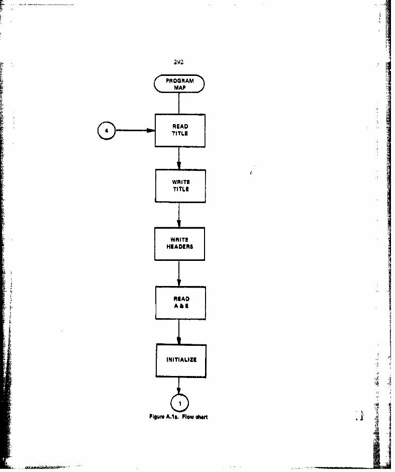
292

PROGRAM

READ

TNITLIE

WRITE-

Tiur IT.LowE ar

293

READ P1110LAMO, P1

Pz, Sc

CONVERTPROM DEGREES

TO RADIANS

READCONTROL

CARDS

Figure A.1b. Flow chart

SUSHOUTlNN

POINT

IIA.P I7 LAM,

W~~ieARD lw hr

CONVIRT7

NAUTH~~ AUHA

IPHIhi,-Tu -

<. 0

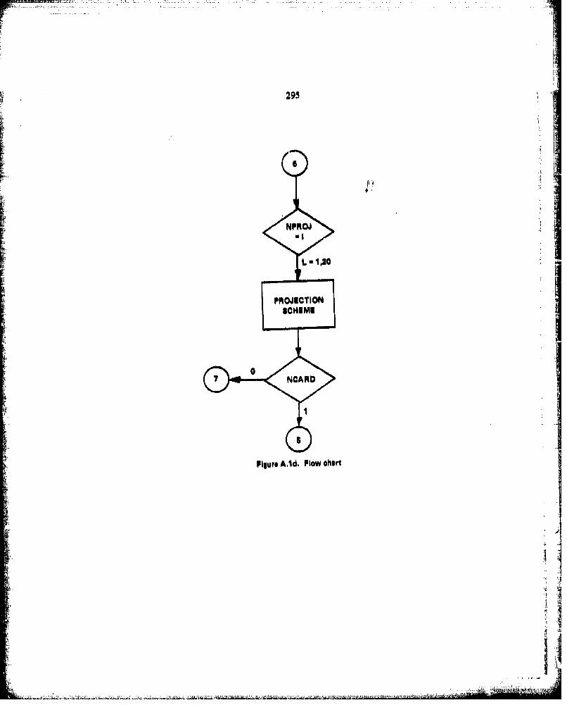
295

$CHIME

Figure kid, Flow chert

296-

3

ORID

SRAD PHI,LAM, OPHI,

CLAM, NPHI,At NLAM

FiueAUT. Plow Aari

SINNING

0Iv.-.".................................................................... -.- i

297

NPROJ

PROJECTION

INCREMINTPHI LAM

LAII

Plpm .1f.Plowaha1

..............

299

PROGRAM m~p COO MEO FTIN V3@0*PJS OCPTai I I

PR04RAMM MAPL llNPUTpOUTPUT9TAPEbsZNPUTs TAPE~uOUTPUfliEAL LAt*~,LAMO~,LAMO

COMMCNiNOUT/PgII~,LAMqM, y

1. F EAO(5j,2) T ItT 29T 39 T4 TO 9T6,TT vTS2 F3UMAT (6A 10

WRITE (up 31LO 3 FOUMAT(IMII

W-71TE (ut,.d TI ,TaT3,T..,TBTb, U ,T

102 O;t'1AT (CX ,6LATITUOCX9HLONGTUO~t$,LM~1HIoiHViM)

I FOqMATt2FiOmfl

ILSAMCNI~~PHOLAOPiP,

26 loPHa.$mP~/RT ULA MCI0mLtiRTOr PHI20uiPRTOkk.A0(f9!) NGASENPROJNPNTNGCNNAUTH

' FONMA1(515h1F(hPhT.sA.iJ CALL GRIOINC(ONiNAUTHiNPROJ)lFlNiPN7.LtJs) GO TO 6CALL FOIN'TMNoNAUTHNPROJ)

b IF(NCAEE~st) GO 10 1is bTCP

ENI

Z

299

Ow kT Iii F~l 11 CJC 6aoO FTN V.3,O-P.380 OPTl it

oRUTN PO~INT (NcON0IAUrHsNFROJ)KEi.L i..MLM.LAMOLAMORLAMTILAMOTCOICNCN1siA, ~,SHZCiLMMOR, ARCPI, PHi ,PH2,RTDC0MMCNlINOUTPIkLAM~,xY

IUS Keu0(6,iO'. PH~lLAMNCARO

LkIM~aLAMIRTO

IF(N^Ufl#Ew,1) OALL AUTHAL(PHIZpPHIZT)IF(NCCN.*.Osi) CALL CONFRMIPhlRPH1TLAM,LAMTLAMOT)lF(NAUTH,..W2..OR*NGONs(A. 1) PNIR*PHITJ.F(hNO.N.lU. LAOIRBLAF'TlFMNUON.Q.i) LAMOARLAMOT

1 CAL.L EQAF AZ ti,2g) Mai

G~O TO to$2 6LL emRCNI

20 GO TO 10!4 aALL 10ARCL

CsO TO 106

CALL PARAS60 TO lot,~. .

7 UA66 SIN4US60 TO 101i

3 L#LL MI.Li.W39(60 TO 105

9) 1 4L HAMME1%40 To 2.O6

10 tA0LL MERCcoo TO too *

LL. CALL STEoLO TO LO

12 QALL LAM13RI(O To ±L)5

LJ CAL.L LAMS8ia 1(.0 to too

1.CALL G NI'6.0 TO ia

la. CZALL A.L8UiOGO TO Los

*0 Lo C&ALL ORTHOCiO TO 10

it LALL SIMCNI(j0 To IOa

18 CALL S:MCN250 GO TO M0

L, -1 L4L SIMOL

20CALL POL Y

05 106 FORMAT4Z4V~sF9.41927k?,7i2m3))

SUBROUiTINE FOINT 000 6600 FTS' Y3*0-P.180 OPTuI IL

IF(NCARqO*EQ~il GO TO 103RETURN

L.4,

mo .iTV

3011SUdRjUfINE GRlJ CDC 6EGO FTtN V3*U-P38J OPT=1i 11.

4kRQUJTlN4 G~l0,(hCNNAUTH#NF'ROJ)REAL LAMLAMRLAMOPLAMORPLAMTpLAMOTpLAMOCOMMON/CNSIT/AESPH1ORLAMOCRRRCPIFH1,PHaRTOCOMMCN/INOUT/PMZR0LAM~sX'Y

S READ(SvI0O PMILAM9DPHI9,ULAMvNPHINLAM103 FORMAT (4 (F1O.4)p2I5)

PHIREPHI/RTOUPHI~3GPHI/RTUOLAM~sOLA M/RTO

±0 L)0 104. I1,NPHIt i4~zLAM/RTD

IF(NAUTH*EU#I) CALL AUTHAL(PHI,PHI4T)IF(NCON*EQ.±) CALL CONFRM(PIRPP'ITLAMRLAMTLAMOT)

IF(NOCNE~e 11 LAMINuLAMTIF(NCC~sE0.i) LAMO~mLAMOTGOTO,,,',,,,,,O1,113l4116118

ICALL EUARAZ lg,20)tNPRO420 Go TO 105

2GALL EARCN1GO TO 10 S

3 CALL EARCN2GO 70 1LU5

25 4 CALL EGARCLGO TO 1O5

CALL WONNEIo CALL P4RA 8

so 40 TO 105?' GALL SINUb

GO TO 105d CALL MCLLW

GO To iOb

9 CAL.L HAMMERIGO TO 105

10 GALL M RCGO TO LOS

11. CALL STEREOGO TO Lob

U~ CALL LAMBRIGO TO 105

13 G;ALL LAMBR2GO TO 105

t41 CALL GNOMGO TO 105

if CALL AZEQUDGO TO 105

16 CALL ORTHOso GO TO L0S

17 CALL SIMONiGO to 105

1.8 CALL SIMCN2GO TO LU&

so L9 CALL STMC L

302

SUaROUTINE GIDt CDC 6400 FTth M3O-P38a OPTmlIJ1

GO TO 106k, ~20 LAL POLY

Lai PH Ion RTo* PHIRL AMc~.RTCILAMR

00WRITE(ttiM6 PHZLILAM09XY*106 FORMAT(Z19XvF9*4),aI7X9Fl2*3))

W0 LAMFRuLAMR+ULAHR10k. PHIRoPHIR+DPHIR

RET URNt'

ENO

303

SUBROUTINE C 04FR M GOO 6,100 FTI V3@0-P.360 OPT8I

S U tiOUTI NE COFMPIoH~ M#ATLMTREA~L LAMRoL.At"RLAMToLAHOT

$NP0*SlN(P1IOR)4NP02zkjNPQSNP0CSPOaCOs (PehZOR)

KPOxA/6QRT(1.-E2SNPO2)

6xSQTil+E2*CSPO4M&(LE2))LA MT=*LA MRL AM CTmiLAM OR5.NPoSIN(PHIR)

FA~t2:ALOG(PZ/4..4PHlR/aO)

PTzATAN (TNPT)PHIT&264PT-PI/2vRETURNEN

SUBROUTINE AUTHAL CDC 6600 FTNi V3*0-P360 OPTu1

SUaROUTIN9 AUThAL (PHI AtP MIT)REehL LANORCOMMOINCNSTIA oft SoPH IOR9LAM OR 9At RCoPlo FMItFH2RTOE2aE*E

b L'.E2*E2It I.6uE2*E4

SNPm I N(P HIR)SNP28SNP*SNP,SNP4PSNPZ*SNP 2

±0 SNP66SNP2*SNP4FAC±.1.* .66667E2*SNP2.6E4SNP4..5?42*Z6*SNPGFA2u1~oI,4. E+b*4eS126ESNPT=SNP#FACIIFAC2PHIT=ASZNISNPTI

±5 RuASRT(iE2441g*.I66667#E2*64E4*571428*ECl)RETURNENO

305

susROOU1Z!E E Q 4R AZ Coc GEoa F~TN V3,0OP3$O OPTNI

SUJROUTINE LOARAZ

/A,, ,PH ICR LAflORR RC ,PPM 1, PHIRTO

rommCN/I NOUT/PHZR, LAMRXYLFtpM1OQRoL~.s1.b

2Q?) Go TO I.FA(mSQRT(2#4lsSINfPHIR)))XmR*4FAO*&OS (LAMR-LAMOR)YwR*S*FAO#$IN( LAMR.LA94OR)KETURN

~SNPSSIN(PHIR)GSPaCOS(PHIR)t .NP0USIM PHIOR)CSF~aCOS (PHI0R)

4N SICS( IAMR-6A0R

IF(PMZRLe..O~ANO*PHIRLE,,0OO±) ALFBPI/Ze

xFiPI0R.L.Eo,OO01.ANPHRLge *000) Go TO 2

ALFoATAN24SNLP (CSP0.SNP/CSP-SNFP0CSLI)2 kH SQRT(2.*(1*SNPOSNPOiCSPC5POCSLI)

20 )ImRSRH*SIN(ALF)

E.NO

SUBROUTINE EARCN1 CDC 6600 PiN V3*0-P3$0 OPT01 -

SUBROQUTINE EARCNIREAL Li4MRPJ.AMORCOMMNNCNST/ACSPH1Z0RLAMCRP RRCPZPM1,PF12,RTDCOf'it4N/NOUT/PH2R9LAMR.K, YSN9POsSZN(PHIZOR)RHQuR*SQRT(1.4SNPO*SNFO-2.*SNPO*SIN(PHIR) I/SIPCXaSiORH04S1N ((LAMR-.A MORI *SNPO II 'rS*(RTAN(PHZOR)-RH0O1COS((LAMR-LAMOR) 'SNPC))RETURN J

10 END

SU8ROWTINE EARGN2 000 6e00 FTN V3**-P38O OPI.±SUbROUTINE EARCN2REAL LAMRLAIIORCOtlNON/CNST/AESPHICR, LAMOR, ftCPI ,PH1,PH2,RTOUOIINON/ NOUUPHZR9LAMR9X9Y

5 SNi~srN(PHI)SN2uSIN(P4ZSMaGOSIPHI)OS28COS(PH2)

Lo ~ RHO22.*RCS21 (SNi+SN2)FACIu.5' (RHOL4RH02)

FA03ud."o(LAMft-LAMCR)0 CSN14#SN2)FAC'.uSQRT (KHO±lftOi+FAC2)

YaSf(FAC1'FAC4*CDSIFAC3))

3O0

SUBRtOUTINE EQAROL CDCOGQ eaTN V3*0-P380 OPTuI. I

SUdROUTINE EQARCL2R'EAL LAIIRLAMOftCOD4MCNICNST/A ,ESPHIXoLAMORRRCPPP1PH2,RTD AGOMNlIZNOlUTPHIR, LAMA9XvV

5 XsR*S*(LAMiR*LAM0R)

RETURN

4

A

4'IM

I.......

309

UdROUTINE LONNL GOC b(00 FTS V3aQ-P380 OPTNI

SUtuROUTINE 6ONNEREAL LAMR9LAMORGOMMCNONSNT/A ,E,5PHIOI~,LAM0I~PRCPtHPHPRT0COMt4CN/1NOUTIPHItLAMRo~tYRHOOW~C0$ IPNHO)/SIN (PHIOR)

YaS(RM0O.I)#QCS((LAMRI.AMR)'COIPi4ZR)9R#RHQ))tK TUR N

~EN

/ I

SUBROUTINE PARAB C00 6600 FIN V3.*P360 OPTal

SUBROUTINE PARABREAL LAMRLAMORCOMMONICNST/lAo K#SvFPIOR9LAMORsRKCt I *PHI9P41RTOC Ot*ONdi NOUT/PhIR PLANO tX iYu * 4SNPI~lRETURNE NO

SudRQUTINE SZNUb C0C 6muu F1N v3I.O-P3so OPTNI.

bWBRQUTINE SINUSREAL LAtIROLAMOR

CC9MCNO'ZNOUVTPMZRoLAIIRSX96 XuRS* (LAMiR-LAMOR)*CO$PHlIR)

V a fk 5PH IRI RE~T URN

E~NO

I.

IEi312

SU JOUTIAE MO06LW C00 6600 FTIN V3*O-P380 OPTaI.

SU6ROUTINE MOLLWREAL LAMRILAMORCOMMICN/CNSTIA ,E,5,PNZO~LAMORRokftCPPN1PH2,RTOCOMMONINOUTIPtIZRLAMA, X,

WSN&'JtPHIR)

I THToTHT*OTHT

Xa (LAMR-LAMQR) P**OSTTIF(ABS(PHIR~)oGtvI.582Q?) KinD.

REUR

LN.1

313

SUd6IOUTIN4i Al 4ML R COG 6600 FTN VaoO-P340 CPTuI.

L~JuROUTINE HAMMER

COMMC~~WCNSITVA ,E,$,PNQRLAMORI#RCPZ, PNIPH2,RTOCPOMMCN/I N0UTIPIILAMRq, V

b IF(AdStAN(PHIR)).LE..OOQIJ ALFmPIV2.1F(A85(TAN(PmIA))sLa*G.OQ) GO TO IALFUAAN24b.N((LAM-LAIQR/2.) TANIP'HZR))IKOaS~r,T(2.9tLoaCCS(HIZR)4COS((LAMR-LAMOI2.o))

VaAPSPrH0'0Q ( ALF)I

1 -

314

bU~jfoUTINE MeI~c CO~OPNV.PS P

WaROUT1NE 14ERGREAL LAMRsLAMQRc~omMON#CNST/AiioPItAMR9RtIFl)ZRTCOM4MCNeZNQUT/PHIR9A'~$9 V

SNPm ISIN(PHAiA)

F A(;Z*TAN (PZ/.,* % PHZR/2 I

LO YsA*SALOGIAI*AZ2)

CSP~kCoS (PhI!R)c.~POscos(PHL.OR)SN CBSZN CP HLU R)iNLE.SIN(LAMROLA40R)C0i6uCM 1AKA-LAOR)IFAFPHZCULi.oOC00) GO TO 2

Ai.FnATAN2 (SNLo (SNPOLk;SL-CSPO4SNP/CSP))

V&A*S*4ALOG1FAG)/2*

2 Xma6*S*ATA1421SNL* SNPICSPI

RETLURN

'SN

315

SUdROUTINE LAM4~R1 COC 6600 FTIh V3oO-P36D CPTouI.

S06~ROUTINE LAMORLkEAL LAMR#LAMORL.CMMCN/CNST/AESPHZORgLAMQI~9 RpRCIPlpPH~gPH2,NTOC0M'MCN/INOUTIPHIRvLAM~vXvYSNPuSINIPIIR)5t4P~mZN (FHZOR)jkP~uA/5QFT( .-E*E*SNPO*SNP0)kH4aRPO*COS(PHI0R) /SNPO

THI. (LAMR-LAMORI*SNPOi.O F ACIaT AN (PZI4 o PHIR/2.

FA(02v TAN (PIJ'. o-PHIORt2 vF AC~a ( (I m 4SNP) I *- E 4SNP 1 * (E/2* IFAC'.. I(1.+E*SNPO)/(1,-64'SNPOI) ) IE/2.)RH~uRHCO* IPACi*FACJ/FAC2#PAC4)'4 SNPO

Is )XuS* (iHC451N(T HT IYtuS* (RHOO-RHO*COS (TI4T IRET URN~ENO

~,,----....,MAI%

316

SU OUT IiL L A ' t2 000 600 FT- VSoO-P360 OlPTxi.1

ioUcROUTINE LAMSR2EA6 LAMRtLAMOiR

COMMCN/I NOUT/PHIR9,LAMR#XOY5 $NPrnSIN(PHiIRJ

SNPIaSIN (Pi)bN02aINO(H2h .

CSPI*COS (Phi)(AP2suS I(PH?)

'10 KP.AISQRT(1.-E*E*SNPI*SNPlJRP~xA/SQRT (1.-E*E*SNP24 SNP2)

FAG~mTAN (P1/to -PM2/2*.

FAC~mANPI/(V P.2P/R2CP2

NifJOFAC5/ALOG (FAC1#FAU;3/FACU/FAGi.),'Slaln2I*CSPI/ (SNPC*FACL*FAC3)THT& (LAMR-LAMOR) *SNPO

RH1.RPI*CSPi/SNPO 41E20)XaS*RHU*SiJ (TlT)YR$* IrqHI-RHU*COS (THiT)RETURN

25 LNU

317

*SL3bROUTINE SRkO CiJC bO FTK V3*0 P 380 0 PTalI

SUQ;ROUTINE STEREOREAL-LAMRoLA40OR

COMMCN/I NQUT/PHZR, LAMRX, YSNPuSIN(PIIIF(FMZCRs.LE~.I.5620F) GO TO I

FAC2u'fAN(P/4e-PHIR/j2a)

X=RHO41COS (THTI F

15 1 CSP=CCL(PH~IKI)SNPOsSIN (PHiIOR)LSt'ORCO'L(PHIOR)C~S 6*0CS ( L~'mR-LAMOR)SNLaSIN( LAMR-LAMOR)

0,, T. URNE4NL

SIB.

SvJ8rOUTINE GNOM COO *000 FTN V3.0-Paso OPTS11 I,

SUBROUTINE GNOMREAL LAMRoLAMORQQANNN/CN-/0A E*5v-OHZCR9LAMOR#R,9RCPoPHI PH29ATDCbA14C N/ I N OUTO'P H IR L A MR p pbNO"UM ~PHI R)CSP*obS(P441R)CSFOuCOS (.PAIRbNL96ZNIAMR LAmoR)

L.0 OSLaC4OS(L.AMR-L.AMOR)Xa**SON/SP*SPG P*$'GLYm**CP*N,-NOCPC*l (SP*N*SOCPCI).

61RET 'JOkLNO

f

&MON

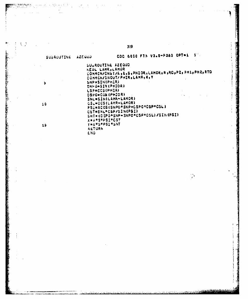
.... .4.

319

SUURO)UTINE. AZFWUJJ C0C 6100 FYN% y3*0-P360 oplul i

WwROUTINE. AZEQUOKEAL LAMRoLAMQRuOM.CN/CNbTA~,SPHIORLAMORRRCDPt9PM1.PTCQMMCNI1NOUT/ PHt~oLAM~, K,SNP-ISIN(PHIR)SNHQ&SJN (PtiIOR)o.SPCCS(PHIRk)

SNLOSZN(LAMk-"LAMOR)la0 C3,.uCCS(IAM-LAMOR)

PSJIACOS(SNPO*SNP4GSPO'CSP*CSLI

SNT. (C SPO*SNPiSNPOCSP*CSL) /SIh (PSI)XBA*SPSI*CSTYaA*S*PSI*SNT

RETUR

320

SUdROUTINE ORTHO COC 6900 Fin V30IP350o ur;3a. I

PEAL LAMRoLAI'IORCOMMCN#CINST/A,~,SPIORLA'OftRfCPI.PM19PI12,RTOCQD'It4N/NOUT/PI{RLAMRX, V

0 SNPoSZN(PNHft)CSP&COS (PHIR)SNPOsSIN (PHIOR)GSPOnCOS (PallOR)SNL~ASItILAMR-I.AMOR)

10 0SL8CQ~lLAMR-LAMOR)lF(A8StPHlOR)*LE.oOG10) GO TO IPS IuACCS (SNPO*SNP4CSPO*CSP*CSL)THImATAN2((CSPO*SNP-SHPO4CSP*CSL),(SNL*CSP)I$N~uSIN (PSI)XmA9S*$NS.ECOS(THT)YsSSN*l(TNTlRETURN

I PSI*ACOS(C'aP*CSL)5NSzSlN(PSl)

20 lF(Ad5(SNLlsLE.t1001) THToPZI2*lF(A8S(SNi.sLE..oOO1) GO TO 2THTmATAN2(TAN(PHZA) ,SNL)

2 XuA*S*SNS*CCS(THTIVf A*S*46S~IN (TNT)

25 kETURNEND

I 321

SUi$ROUTZN4 9.MGNI 000 6400 FTK V3*0-P380 OTI)

SUdRtOUTINE SIMNNPIAL LAtiRILAMOR

RETURN $SIt4IP14%CR)I I

END

U4

tI

322

SUMRUTINE SZMCN2 CDC bbaa FTN V3*0-P380 OPTa I

aw SUUROUTINE SIMCN26,EAL LAPIRLAMORrCOMMONIICNSTiAtEsPMIORLAMOR,~RCPiPiItPH2,RTDC 0M M 0N /I NOU TIP HI R LAM R X, V

I i SplacOs(PHII1

GlSPC 02)/(PHfoP2i

RH$Iu(PH2-PM1)/ t1.-CSP2/GSPi)

toX.A*S 4 RHO 4 SIN ((LAMR-LAMOR) MCl)VaA'S*(RHI1RHO*COS ((LAMR-LAMOR)*C1 I)RETURhENLJ

323

SUdROUTINE SIMOL CDC 6100 FTh V3*O-P3SO PMl I

4UBROUTINE SIMCL

CONiMCN/CNSTIAE, 5,PHZCR ,LAMOCRAIfCP! ,FfrlPN2,RIDCOMMCNNOUTP4IRpLARoxty

b XzA*(LAMRLAMO)'PI*2VSA*S*PHIRRETUR'NEND

A i

4 ;V) 44

324

SUcsRJTINE POi..V COO 600 FTN V3@O-P360 OPTuI

SUAG~UTINE POLYREAL LAtIRLAMORCOOMlCNlNST/AESPHIQRLAMO~, ARCPZ, PH1,PH1,NTOCQMMW~Z NOUTlPIRvLAMR9XsgY

5 IF(PHI4RoNE*Q.l GO TO I

XAA*S* (LAMR-LAM4ORIRETURN

10 SNPoSIN(PHIR)SNi..SZN( (LAAR-LAMOR)*SNP)GSLuCCQ( L.MR-LAM0R)*SNPIX aA 6S 4CS P 0SNL ISN PYaA*S* (PH ZK-PHXORCSPO(1.-CSL I /SNP)

15 RETURNE.NO

Appendix A.2

ANCILLARY PROGRAMS

alFour ancillry programs were required to generate thle tables or Chapter 3. These are IGEOCEN, CUR VA, MERID, and CIRCLE. These programs are Included In this appendix.

In ll f te pogams DLHI s tleinurement iii latitude In radians, and DLPHID Is theofteeprograms have thle constants ortl G-2spheroidInlddnthm

GEOCEN gives geocentric latitude us a function of geodetic latitude, and geodeticlatittude as a function of geocontric latitude. CURVA calculates tile radii of curvature in-themneridianal plane, and perpendiculnr to the muoridianal plane, in it function of thle geodeticlatitude. MERID produces thie distance along the mieridionial ellipse correspondinig to V' ofare as a function of geodetic latitude, Finally, CIRCLE gives the distance iilonyigit circle (it'parallel corresponding to I' or tire as a function of geodetic latituide.

J

jiI

326

PROGRAM GUFVA COG 0600 FTN V3*0-P

PROGRAM CUqRA(INwUTt0UTFUT1POINT I

I FORMAT(1HI

5 A063780659PHIUO.PiHT0D111OLPH Iao.0 72O65OLPH!O .5.

lUE2 sE'FACuLs-E200 a I1919SNsSIN MP141)SN2aSN 'SN

IS RPOA/SQRT(1..-E2*SN2)

PRINT 3,PHlOoRPRM3 FORMAT (5XP6sI,5X9F9 40,9.0

PIsIPHI+DLPHI20 1 PHI~aPHIO.DLPHID

ST OP

... ... - -. M

327

PROGRAM GEOCEN 000 b600 FTN Y3*0-P38

PROGRAM GEOCEN(INPU1~,OUTPJT)PHIaiiPHIOU40

F. Em l, Sidir 5 OELPHIs.W2665

FA~u5QRT (L.-E*E)PRINT 3

5 FOIRMATU.H11

TPPuFACTAN (PHZ)TPaTAN(PHII/FACPPLREATANfrPP)*57.zgssP0mA TAN UP )*5?s2956

5 PRZNT &*PHIOPPOPH1DPO2 FORMAT 12XFb*295XsFB o v 6 X 9F 0 v2 9 9x $ a 4

Pt4Z~uPHIU.CJLPHDI, PHaPH+DLPHI w

20 ENO

q 1

328

PROGRAM MERI D COO 6600 FTN V390-P

PUR3~AM MERZO U.NPUTsQUTPJT)

#F~m35#*v6/30?2s

30 t INLO19

20 PHMfvPZ.1.I.5444IE-04K SN2o'"(OS(PH12+PHZ1)*SIN('MZ2-PHNZ±))

)UAUt(PH2PimC2SN23SNCFIMSN6)25 OR14T 31 PH13PO,

4.3 FO*4Ar (5X9F.Qs5XF9v3)PHZ'RHI0L PHIt

2 PNI3nPHIO*0LPHIDST OP

329

P R RA M CIRCLE 000 6600 FTN V3eQ-P3$k

PROGRAM CIRCLE (INPUTCUTPUT)

Au6378165.I3LA'2 .94i86SE-4

B PHImO.PHI~xO.

PRINT i10 1 FORMATU1H11

00 a Zul,9SNPmSZNIP41)SN2sSNP*SNPOnAk'DLAM4COS(PHZI SQRT11 ii." 'SN21PRINT 3, PH1OD

3 FORMAT MoF6 2 P5,F9, 31PI4IaPHZ *OLPHZ

a Pt4Z~uPHID4OLPMlW

20 ENO

DISTRIB~UTION

I )Vele I.OCUMCenttiOnl Center(am er1oli StationAkxandria, VA 22314 (2

Dofeinse Printing ServiceWashington Navy YardWashington, D 07

Library of CongressWashington, D)C -20540ATT"IN: Oift and I xchango Di'vision (4)

lDefenge Mapping AgencyWasington, D)C 20360

Defense Mapping Agency To'(pographic CenterWashington, DC 20315

DuComoas Ma pping Agoncy Aerospace ConterSt. L.o1s, MO) 63118

lOee m Mapping Agency H]ydrographlc Center.Washiington, DC 20390

Englncerlng Topographic LuboratoryFt Bolvoir, VA 22060

Notional COcounic and Atmospheric Adin.National (.)can SarveyRockvlle, MD) 20850

Vpi & skiFISM Dept (Dr, L Merrovitch)tBlockiburg, VA 24060 (4)

_W,1

... ....................... .................... ------------

DK-1O0 (20)

DN-80 (2)DN-8J (I'oarson) (45)DX-21 (2)DX-222 (6)DX-4ODX-43 (Aids) 4

"Mm1