properties, estimation and application to financial …
TRANSCRIPT

Advances and Applications in Statistics
© 2021 Pushpa Publishing House, Prayagraj, India
http://www.pphmj.com
http://dx.doi.org/10.17654/AS071010055
Volume 71, Number 1, 2021, Pages 55-84 ISSN: 0972-3617
Received: March 17, 2021; Revised: April 22, 2021; Accepted: October 10, 2021
2020 Mathematics Subject Classification: 62P05.
Keywords and phrases: modified Bessel function of the third kind, generalized inverse
Gaussian distribution, generalized hyperbolic distribution, EM-algorithm.
∗Corresponding author
Published Online: November 16, 2021
PROPERTIES, ESTIMATION AND APPLICATION
TO FINANCIAL DATA FOR GENERALIZED
HYPERBOLIC DISTRIBUTION WHEN
THE INDEX PARAMETER IS 2
3−
Calvin B. Maina1,*
, Patrick G. O. Weke2, Carolyne A. Ogutu
2 and
Joseph A. M. Ottieno2
1Department of Mathematics and Actuarial Science
Kisii University
P. O. Box 408-40200, Kenya
e-mail: [email protected]
2School of Mathematics
University of Nairobi
Kenya
Abstract
Generalized Hyperbolic Distribution (GHD) arises as a normal
variance-mean mixture with Generalized Inverse Gaussian (GIG) as
the mixing distribution. The GHD nests a number of distributions
obtained as special and limiting cases. In literature, however, Normal
Inverse Gaussian (NIG) and Variance-Gamma (VG) are the most
commonly used special and limiting cases, respectively, in analyzing
C. B. Maina, P. G. O. Weke, C. A. Ogutu and J. A. M. Ottieno 56
financial data. The objective of this paper is to derive another special
case of the GHD, obtain its properties, estimate its parameters and
then apply it to some financial data. The properties are determined by
first expressing them in terms of the corresponding properties of the
mixing distribution. The maximum likelihood estimates are obtained
using the Expectation-Maximization (EM) algorithm which overcomes
numerical difficulties occurring when standard numerical techniques
are used. An application to a dataset concerning the Range Resource
Corporation (RRC) is given. It is shown that the proposed model
captures the skewness and excess kurtosis exhibited by the data. The
maximum likelihood estimates are shown to be obtained easily by the
EM-algorithm.
1. Introduction
A normal distribution has two parameters: the location parameter
representing the mean and the scale parameter representing the variance. For
a continuous mixture, we can fix the mean and vary the variance and vice-
versa. Barndorff-Nielsen [2] introduced a normal mixture where the mean is
a linear function of a varying variance. This is called a normal variance-
mean mixture. When the mixing distribution is Generalized Inverse Gaussian
(GIG), then the mixture is called Generalized Hyperbolic Distribution
(GHD) which nests a number of distributions obtained as special and
limiting cases. Special cases are obtained when the index parameter λ takes
specific values. When ,1=λ we obtain the hyperbolic distribution which
was the first special case used in financial modelling (Eberlein and Keller
[4]). Later on, Barndorff-Nielsen [2] introduced the case when 2
1−=λ
which is the Normal Inverse Gaussian (NIG) distribution. The NIG has been
extensively studied in finance because of its analytical tractability property.
Prause [7] mentioned the case when 2
3−=λ and obtained the mean and
variance and no further work has been done. It is the objective of this
paper to study this special case in detail. The specific objective is to
construct, obtain properties, estimate parameters and apply the model to

Properties, Estimation and Application to Financial Data … 57
Range Resource Corporation financial data. The Maximum Likelihood (ML)
parameter estimates are obtained via the EM-algorithm.
This paper is organized as follows. In Section 2, we have definitions and
properties of modified Bessel function of the third kind. Section 3 deals with
the generalized inverse Gaussian distribution with its special case. Section 4
covers the mixed model and its properties. Parameter estimation based on the
EM-algorithm is covered in Section 5. Data analysis is performed in Section
6 and the conclusion is provided in Section 7.
2. Modified Bessel Function of the Third Kind
The most important mathematical tool used for this work is the modified
Bessel function of the third kind. Its definitions and properties are given in
this section. For more detailed study, see Abramowitz and Stegun [1].
Definition 1 and its properties
Modified Bessel function of the third kind of index λ evaluated at ω
denoted by ( )ωλK is defined by
( ) ∫∞ −λ
λ
+ω−=ω
0
1 .1
2exp
2
1dx
xxxK (1)
An alternative form of Definition 1 is
( ) ∫∞ −λ−
λλ
ω−−
ω=ω
0
21
4exp
22
1dt
tttK (2)
which is obtained by letting .2t
xω=
Some properties are as follows.
Property 2.1 (Symmetry)
( ) ( ).ω=ω λ−λ KK (3)

C. B. Maina, P. G. O. Weke, C. A. Ogutu and J. A. M. Ottieno 58
Property 2.2 (Derivative I)
( ) ( ) ( )[ ].2
111 ω+ω−=ωω∂
∂−λ+λλ KKK (4)
Property 2.3 (Derivative II)
( ) ( ) ( ).1 ω−ωωλ=ωω∂
∂+λλλ KKK (5)
Property 2.4 (Recursive relation)
( ) ( ) ( ).211 ω−ω=ωω
λ−λ+λλ KKK (6)
Definition 2 and its properties
( ) ( )∫∞ ω−−λ
λλ −
+λΓ
Γ
ω=ω
12
12 .1
2
1
2
1
2dtetK
t (7)
This can also be expressed in summation form as given below:
Proposition 1.
(a)
( ) ( )∑∞
=
−ω−λ ω
+λΓ
++λΓ
−+λΓ
+λΓ
ωπ=ω
0
2
2
1
2
1
2
1!
2
1
2i
ii
ii
eK (8)
( )
ω
+λΓ
−+λΓ
++λΓ
+λΓ
+ωπ= ∑
∞
=
−ω−
1
2
2
1
2
1
2
1!
2
1
12
i
ii
ii
e (9)
which can further be expressed as
(b)
( ) [ ( ) ]( )
.8!
1241
21 1
22
ωΓ−−γ+ω
π=ω ∑∏∞
= =
ω−λ
i
n
in
n
ieK (10)
Properties, Estimation and Application to Financial Data … 59
Proof.
( ) ( )∫∞ ω−−λ
λλ −
+λΓ
Γ
ω=ω
12
12 .1
2
1
2
1
2dtetK
t
Let ( ).1−ω= ty Then
( ) ( ) ( )∑∞
=
−ω−λλλ
λλλ
++λΓω
−λω
ω
+λΓ
Γω
ω=ω0
2
12
2
122
1
2
2
2
1
2
1
22
2
i
ii
ieK
( )
ω
−+λΓ
++λΓ
+ωπ= ∑
∞−λ
=
−ω−
1
2
2
1!
2
1
12
i
i
ii
i
e
( )( ) ( )
ω
−+λΓ
++λΓ
+ω−λ+ω
π= ∑∞
=
−ω−
2
2
2
2
1!
2
1
8!1
141
2i
i
ii
i
e
( )( )
( ) ( )( )
ω−λ−λ+ω
−λ+ωπ= ω−
2
222
8!2
9414
8!1
141
2e
( )
ω
−+λΓ
++λΓ
+∑∞
=
−
3
2
2
1!
2
1
i
i
ii
i
( )( )
( )( )( )
ω−λ−λ+
ω−λ+
ωπ= ω−
2
222
8!2
9414
8!1
141
2e
( ) ( ) ( )( )
( )
ω
−+λΓ
++λΓ
+ω
−λ−λ−λ+ ∑∞
=
−
33
222
2
2
1!
2
1
8!3
2549414
i
i
ii
i
C. B. Maina, P. G. O. Weke, C. A. Ogutu and J. A. M. Ottieno 60
( )( )
( ( ) )( )
ω−−λ+
ω−λ+
ωπ= ∏
=
ω−2
12
222
8!2
124
8!1
141
2k
ke
( ( ) )( )
( ( ) )( )∏ ∏
= = ω−−λ+
ω−−λ+
3
1
4
14
22
3
22
8!4
124
8!3
124
k k
kk
( ) ,2
2
1!
2
1
5
ω
−+λΓ
++λΓ
+∑∞
=
−
i
i
ii
i
and therefore
( ) ( ( ) )( )
.8!
1241
21 1
22
ω−−λ+ω
π=ω ∑∏∞
= =
ω−λ
i
i
ki
i
keK
Corollary 2.1. For positive integers ,1,2
1 −=−λ nn
(a)
( ) ( )( ) ( ) .2
!!
!1
212
1
ω−
++ωπ=ω ∑
=
−ω−+
n
i
i
n ini
ineK (11)
(b)
( ) ( )( ) ( ) .2
!1!
!11
2
1
12
1
ω−−
−++ωπ=ω ∑
−
=
−ω−−
n
i
i
n ini
ineK (12)
Corollary 2.2. When ...,,3,2,1=n we have
(a) ( ) ( ) ,2
2
1
2
1ω−
− ωπ=ω=ω eKK (13)
(b) ( ) ( ) ,1
12
2
3
2
3
ω+ωπ=ω=ω ω−
−eKK (14)
(c) ( ) ( ) ,33
12 2
2
5
2
5
ω+ω+ω
π=ω=ω ω−−
eKK (15)

Properties, Estimation and Application to Financial Data … 61
(d) ( ) ( ) ,15156
12 32
2
7
2
7
ω+
ω+ω+ω
π=ω=ω ω−−
eKK (16)
(e) ( ) ( ) ,1051054510
12 432
2
7
2
7
ω+
ω+
ω+ω+ω
π=ω=ω ω−−
eKK (17)
(f) ( ) ( ) .94594542010515
12 5432
2
9
2
9
ω+
ω+
ω+
ω+ω+ω
π=ω=ω ω−−
eKK (18)
3. Special Case of Generalized Inverse Gaussian Distribution
In this section, we derive the distribution of ( )γδλ ,,GIG and deduce
the special case when .2
3−=λ
Proposition 2. The distribution of ( )γδλ ,,GIG is given by:
( ) ( ) .2
1exp
22
21
γ+δ−δγ
δγ=
λ
−λλz
zK
zzg (19)
Hence, for ,2
3−=λ
( )( )
( ) .2
1expexp
12
22
2
53
γ+δ−δγ
δγ+πδ=
−z
zzzg (20)
Proof. From equation (1),
( ) ∫∞ −λ
λ
+ω−=ω
0
1 .1
2exp
2
1dx
xxxK
Using the parametrization δγ=ω and the transformation ,zx δγ= we
obtain
( ) ,2
1exp
2
1
0
22
1
∫∞ −λ
λλ
γ+δ−
δγ=δγ dzz
zzK

C. B. Maina, P. G. O. Weke, C. A. Ogutu and J. A. M. Ottieno 62
( )∫∞
λ
−λλ
γ+δ−δγ
δγ=
0
221
.2
1exp
21 dzz
zK
z
Thus
( ) ( )
γ+δ−δγ
δγ=
λ
−λλz
zK
zzg
221
2
1exp
2
is a pdf known as the generalized inverse Gaussian distribution.
When ,2
3−=λ using equation (12), we have
( ) ( )
γ+δ−δγ
δγ=
−
−−−z
zK
zzg
22
2
3
12
3
2
3
2
1exp
2
γ+δ−
δγ+δγπ
δγ=
δγ−
−−z
ze
z 222
5
2
3
2
1exp
11
22
( ).
2
1exp
12
22
2
53
γ+δ−
δγ+πδ= δγ−
zz
ez
Proposition 3. (a) The rth moment of the ( )γδλ ,,GIG distribution is
given by
( ) ( )( ) .δγ
δγ
γδ=
λ+λ
K
KZE r
rr (21)
(b) When ,2
3−=λ
( ) ,1
2
δγ+δ=ZE (22)
( )( )
,1
2
3
δγ+γδ=Zvar (23)
( ) ( )( )
,1
3133
362533
3δγ+γ
γδ−γδ−δγ+δ=µ Z (24)

Properties, Estimation and Application to Financial Data … 63
( )( )
.1
31231545
343625
4δγ+γ
δ+γδ+γδ+γδ=µ Z (25)
Proof. For part (b), we have
Mean
( )( )
( )δγ
δγ
γδ=
2
3
2
1
K
K
ZE
.1
2
δγ+δ=
Variance
( ) ( ) ( )2
43
11 δγ+δ−δγ+γ
δ=Zvar
( ).
12
3
δγ+γδ=
Third Central Moment
( )( ) ( )3
6
2
5
3
3
31
2
1
33
δγ+δ+
δγ+γδ−
γδ=µ Z
( )( )
.1
3133
362533
δγ+γγδ−γδ−δγ+δ=
Fourth Central Moment
( )
( ) ( )( ) ( )
( )45
5847325
33425
41
31614
133
δγ+γγδ−δγ+γδ+δγ+γδ−
δγ+δ+γδ+γδ
=µ Z
( ).
1
31231545
343625
δγ+γδ+γδ+γδ+γδ=

C. B. Maina, P. G. O. Weke, C. A. Ogutu and J. A. M. Ottieno 64
4. Proposed Mixed Models
In this section, we construct the normal variance-mean mixture when the
mixing distribution is .,,2
3
γδ−GIG Then we obtain the properties of the
mixed model. The construction can be made through the following:
Proposition 4. If the conditional distribution ( )zzNZX ,~ β+µ and
,,,2
3~
γδ−GIGZ then the mixed model is given by
( ) ( ) ( ) ( ) ( ( ) )( )
,1
expexp
22
2
1
21222
β−αδ+π
αδφφββµ−β−αδδα=−
xKxxxf (26)
where
( ) ( ) .1 22 δµ−+=φ xx (27)
Proof.
( )( )( )
( )∫∞ β+µ−−
π=
0
2
1 2
2
1dzzge
zxf z
zx
( ) ( )
( )δγ+πδγδ=
µ−β
12
exp3 xe
( ) ( )( )∫
∞ −
γ+βδ+µ−+γ+β−×
0 22
22223 .
1
2exp dz
z
xzz
Let
( )( )
.22
22
tx
zγ+β
δ−µ−=

Properties, Estimation and Application to Financial Data … 65
Then
( ) ( ) ( )
( )( )
( ) 22
223
12
exp
δ+µ−γ+β
δγ+πδγδ=
µ−β
x
exf
x
( ) ( )∫
∞ −
+×δ+µ−γ+β×
0
22223 1
2exp dt
tt
xt
( ) ( )
( )( )
( ) 22
223
1
exp
δ+µ−γ+β
δγ+πδγδ=
µ−β
x
ex
( ( ) ( ) ).22222 δ+µ−γ+β× − xK
Write .222 γ+β=α Then
( ) ( ) ( ) ( ) ( ( ) )( )
,1
expexp
22
2
1
21222
β−αδ+π
αδφφββµ−β−αδδα=−
xKxxxf
( ) ( ).1
2
2
δµ−+=φ x
x
One of the attractive features of constructing a distribution by mixing
is that the properties of the mixed model are expressed in terms of the
properties of the mixing distribution. When ( ),~ ZNZX β+µ we have the
following.
Proposition 5.
( ) ,2
2
+β= µ t
tMetM Zt
X (28)
( ) ( ),ZEXE β+µ= (29)
( ) ( ) ( ),2ZvarZEXvar β+= (30)
( ) ( ) ( ),3 33
3 ZZvarX µβ+β=µ (31)
( ) ( ) ( ) [ ] ( ) [ ].366 223
24
44 ZEZvarZEZZX +β+µβ+µβ=µ (32)
C. B. Maina, P. G. O. Weke, C. A. Ogutu and J. A. M. Ottieno 66
Proof.
Part 1.
( ) ( ) ( )∫ ∫∞ ∞
∞−β+µ=
0,; dzzdxfzzxfetM ZN
txX
( )∫∞µ
+β=
0
2
2exp dzzfz
tte Z
t
.2
2
+β= µ t
tMe Zt
Part 2.
( ) ( )
µ+
+β=
+β
µ
+β
µZ
tt
tZ
tt
tIX eEeZetEetM
22
22
[ ] ( )0IXMXE =
[ ]ZEβ+µ=
which can be obtained using conditional expectation approach given by
[ ] ( )ZXEEXE =
[ ]ZE β+µ=
[ ].ZEβ+µ=
Part 3.
( ) ( ) ( )
+βµ+
+β=
+β
µ
+β
µZ
tt
tZ
tt
tIIX ZetEeZetEetM
22
22
( ) .222
22
+βµ+
µ+
+β
µ
+β
µZ
tt
tZ
tt
tZetEeeEe

Properties, Estimation and Application to Financial Data … 67
Therefore,
( ) [ ] [ ] [ ] [ ]( )2222 2 XEZEZEZEXvar β+µ−µβ+β+µ+=
[ ] [ [ ] ( ) ]222ZEZEZE −β+=
[ ] ( ).2ZvarZE β+=
By the conditional expectation approach, we have
( ) ( ) ( )ZXvarEZXEvarXvar +=
( ) ( )ZvarZE β+µ+=
( ) ( ).2ZvarZE β+=
Part 4.
( ) ( [ ] [ ] ) ( [ ] [ ] [ ] [ ] )3233223 233 ZEZEZEZEZEZEX +−β+−β=µ
( ) ( )ZZvar 333 µβ+β=
( ) ( )
µ+
+βµ=
+β
µ
+β
µZ
tt
tZ
tt
tIIIX ZeEeeZtEetM
2222
22
33
( ) ( )
+βµ+
+β+
+β
µ
+β
µZ
tt
t
tt
tZetEeZeZtEe
2222
22
33
( ) ,23233
22
µ+
+β+
+β
µ
+β
µZ
tt
tZ
tt
teEeeZtEe
( ) [ ] [ ] [ ]ZEZEXEMIIIX µ+µβ+µ== 330 2233
[ ] [ ] [ ]3322 33 ZEZEZE β+βµ+β+

C. B. Maina, P. G. O. Weke, C. A. Ogutu and J. A. M. Ottieno 68
( ) ( ) ( [ ] [ ] [ ]) [ ]( )ZEZEZEZEXEXE β+µµβ+β+µ+= 22222
[ ] [ ] [ ] [ ]22223 2 ZEZEZEZE β+βµ+µβ+µ+µ=
[ ] [ ] [ ] [ ] ,222232
ZEZEZEZE µβ+β+βµ+
[ ] [ ] ( ) [ ] .333322233
ZEZEZEXE β+µβ+βµ+µ=
Therefore,
( ) ( [ ] [ ] ) ( [ ] [ ] [ ] [ ] )3233223 233 ZEZEZEZEZEZEX +−β+−β=µ
( ) ( ).3 33
ZZvar µβ+β=
Part 5.
( ) ( )
+βµ=
+β
µZ
tt
tIVX eZtEetM
2222
2
3
( ) ( )
+β++βµ+
+β
+β
µZ
ttZ
tt
teZteZtEe
22233
22
23
( )
×+βµ+
µ+
+β
µ
+β
µZ
tt
tZ
tt
teZtEeZeEe
2222
22
33
( )
+βµ+
+β
µZ
tt
teZtEe
22
2
( )
++β+
+β
+β
µZ
ttZ
tt
teZeZtEe
22232
22
3
Properties, Estimation and Application to Financial Data … 69
( )
+βµ+
+β
µZ
tt
tZetEe
23
2
3
( )
+×+βµ+
+β
+β
µZ
ttZ
tt
tZeeZtEe
22222
22
3
( )
+βµ+
+β
µZ
tt
teZtEe
233
2
( ) ( )
+β++β+
+β
+β
µZ
ttZ
tt
teZteZtEe
232244
22
3
( ) .2324
22
+βµ+
µ+
+β
µ
+β
µZ
tt
tZ
tt
tZetEeeEe
Therefore,
[ ] [ ] [ ] [ ] [ ]233222344 12464 ZEZEZEZEXE µβ+µβ+βµ+βµ+µ=
[ ] [ ] [ ] [ ]442322 366 ZEZEZEZE β++β+µ+
since
( ) [ ( )( ) ]44 XEXEX −=µ
[ ] [ ] [ ] [ ] [ ] ( )[ ] ,36442234
XEXEXEXEXEXE −+−=
where
( ) ( ) [ ]( ) ( [ ] [ ] [ ]22233 333 ZEZEZEZEXEXE β+µ+µβ+µβ+µ=
[ ] [ ])3323 ZEZE β+βµ+

C. B. Maina, P. G. O. Weke, C. A. Ogutu and J. A. M. Ottieno 70
[ ] [ ] [ ] [ ]ZEZEZEZE βµ+µβ+µ+βµ+µ= 3222224 3333
[ ] [ ] [ ] [ ] [ ]223333 33 ZEZEZEZEZE µβ+µβ+βµ+µβ+
[ ] [ ] [ ] [ ] [ ],33 3422222ZEZEZEZEZE β+βµ+β+
( ) ( ) [ ] [ ] [ ] [ ]23222422222 ZEZEZEZEXEXE µ+βµ+βµ+µ+µ=
[ ] [ ] [ ] [ ] [ ]ZEZEZEZEZE23323 2222 µβ+βµ+µβ+βµ+
[ ] [ ] [ ]222322224 ZEZEZE βµ+β+βµ+
[ ] [ ] [ ] ,233224
ZEZEZE µβ+β+
[ ] [ ]( ) [ ] [ ]222344464 ZEZEZEXE β+µ+βµ+µ=β+µ=
[ ] [ ] .44433
ZEZE β+µβ+
Therefore,
( ) [ [ ] [ ] [ ] [ ] [ ] [ ] ]4223444 364 ZEZEZEZEZEZEX −+−β=µ
[ [ ] [ ] [ ] [ ] ]3232 236 ZEZEZEZE +−β+
[ ][ [ ] [ ] ] [ ].36 2222ZEZEZEZE +−β+
Finally,
( ) ( ) ( ) [ ] ( ) [ ]223
24
44 366 ZEZvarZEZZX +β+µβ+µβ=µ
which completes the proof.
Corollary 4.1. When ,,,2
3~
γδ−GIGZ we have
(1) ( ) ,1
2
δγ+βδ+µ=XE
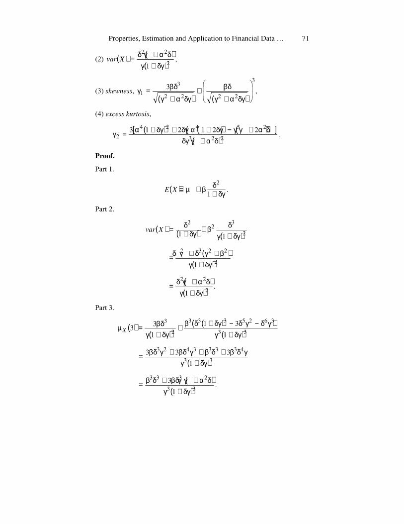
Properties, Estimation and Application to Financial Data … 71
(2) ( ) ( )( )
,1
2
22
δγ+γδα+γδ=Xvar
(3) skewness, ( ) ( )
,3
3
2222
3
1
δγα+γ
βδ+δγα+γ
βδ=γ
(4) excess kurtosis,
[ ( ) ( ( ) ( ))]( )
.221213
223
23424
2δα+γδγ
δα+γγ−δγ+αδγ+δγ+α=γ
Proof.
Part 1.
( ) .1
2
δγ+δβ+µ=XE
Part 2.
( ) ( ) ( )2
32
2
11 δγ+γδβ+δγ+
δ=Xvar
( )( )2
2232
1 δγ+γβ+γδ+γδ=
( )( )
.1
2
22
δγ+γδα+γδ=
Part 3.
( )( )
( ( ) )( )33
3625333
2
3
1
31
1
33
δγ+γγδ−γδ−δγ+δβ+
δγ+γβδ=µX
( )33
43333423
1
333
δγ+γγδβ+δβ+γβδ+γβδ=
( )( )
.1
333
2333
δγ+γδα+γγβδ+δβ=

C. B. Maina, P. G. O. Weke, C. A. Ogutu and J. A. M. Ottieno 72
Therefore, denoting skewness by ,1γ we get
( )
( )( )2
3
2
31
X
X
µ
µ=γ
( )( )
( )2
323
32
3
33
43333423 1
1
333
δα+γδ
δγ+γ×δγ+γ
γδβ+δβ+γβδ+γβδ=
( )
( )2
322
332233
δγα+γ
δβ+δγα+γβδ=
( ) ( ).
33
2222
3
δγα+γ
βδ+δγα+γ
βδ=
Part 4. Note that
( )( )45
3436254
41
312315
δγ+γδ+γδ+γδ+γδβ=µ X
( )( ) ( ) ( )δγ+γ
δ+δγ+γ
δβ+δγ+γ
γδ−γδ−δγ+δβ+1
31
61
316
3
3
52
33
3625332
( )( )
( )45
332222322
332334
1
3416
1453
δγ+γγδ+γδ+γδ+δγ+δγβ+
+δγ+γδ+γδδβ
=
( )( )
.1
331345
332243
δγ+γγδ+γδ+δγ+γδ+
Hence, the kurtosis is given by
( )( )( )
( ) ( )( )
δγ+γγδ+γδ+δγ+δγβ++δγ+γδ+γδδβ=
µµ
45
3322322332334
22
4
1
44161453
X
X
( )( )
( )( )
.1
1
3313224
42
45
332243
δα+γδδγ+γ×
δγ+γγδ+γδ+δγ+γδ+

Properties, Estimation and Application to Financial Data … 73
Writing
,222 γ+δ=α
,2 42244 γ+γβ+β=α
we have
( ) .222 73532334624225223 γδ+γδβ+γδβ+γβ+γδβ+δγ=δα+γδγ
Denoting excess kurtosis by ,2γ we obtain
[]
( )223
6254422
322244224
226
82453
δα+γδγγδ+δγ+γ+γδβ+
δγβ+γβ+β+δγβ+γδβ
=γ
[ ( ) ]( )223
42232422424 442413
δα+γδγγδβ+δγβ+δγβ+γδβ+δγ+α=
[ ( ) ( ( ) ( ))]( )
.221213
223
23424
δα+γδγδα+γγ−δγ+αδγ+δγ+α=
Table 1. A summary of the theoretical property of the proposed mixed
model
Item Description Expression
1 ( )XE δγ+
βδ+µ1
2
2 ( )Xvar ( )( )2
22
1 δγ+γδα+γδ
3 Skewness, 1γ
( ) ( )
3
2222
33
δγα+γ
βδ+δγα+γ
βδ
4 Excess kurtosis, 2γ [ ( ) ( ( ) ( ))]
( )223
23424 221213
δα+γδγδα+γγ−δγ+αδγ+δγ+α

C. B. Maina, P. G. O. Weke, C. A. Ogutu and J. A. M. Ottieno 74
5. Parameter Estimation
Parametric methods commonly used in statistical inference are Method
of Moments (MoM) and Maximum Likelihood (ML) method. However,
these methods have some limitations. Equations obtained by these methods
require complex numerical techniques to solve in cases where the parameters
are hard to separate.
Alternative simple methods have been sought. One such method is
the EM-algorithm which was introduced by Dempster et al. [3] for ML
estimation for data containing missing values or data that can be considered
as producing missing values. Karlis [5] pointed out that the mixing operation
can be considered responsible for producing missing data. The statistical
beauty of the EM-algorithm is that it estimates the unobserved values using
the posterior expectations.
It becomes easier if we exploit the normal variance mean structure of the
GHD through this algorithm. Assume that true data are made of observed
part X and unobserved part Z. This then ensures that the log likelihood of the
complete data ( ),, ii zx ni ...,,3,2,1= factorizes into two parts (Kostas
[6]). The EM-algorithm consists of two main steps: the maximization step
which optimizes the log likelihood with respect to the parameters and the
expectation step which estimates the unobserved values using the posterior
expectations. This implies that the joint density of X and Z is given by:
( ) ( ) ( )., zgzxfzxf =
Therefore, the likelihood function for the joint data becomes:
( ) ( ) ( )∏ ∏= =
=µδβαn
i
n
i
iii zfzxfL
1 1
,,,
and the log likelihood
( ) ( ) ( )∑ ∑= =
+=µδβαn
i
n
i
iii zfzxfl
1 1
loglog,,,
( ) ( ).,, 21 γδ+βµ= ll

Properties, Estimation and Application to Financial Data … 75
For these models,
( ) ( ) ( )∑ ∑
= =
β−µ−−−π−=βµn
i
n
ii
ii z
zxz
nl
1 1
2
1 .2
1log
2
12log
2, (33)
M-step
In this step, the log likelihood of the conditional distribution is optimized
with respect to its parameters :, βµ
( ) ( ),,
1
1 ∑=
β−µ−=βµβ∂∂ n
i
ii zxl
( ) ( )∑=
β−µ−=βµµ∂∂ n
ii
ii
z
zxl
1
1 .,
Equating these equations to zero and solving simultaneously, we obtain
∑
∑ ∑
=
= =
−
−=β
n
i i
n
i
n
i ii
i
zzn
zx
z
x
1
1 1
1
1
ˆ
and hence
.ˆ zx β−=µ
Therefore, at the kth iteration of the algorithm, the estimates for β and µ are
given by
( ) ,1
1
ˆ
1
1 11
∑
∑ ∑
=
= =+
−
−=β
n
i i
n
i
n
i ii
i
k
zzn
zx
z
x
(34)
( ) ( ) .ˆ 11zx
kk ++ β−=µ (35)
The case when
γδ− ,,
2
3~Z
The log likelihood of the mixing distribution ( )γδ,2l is also optimized
with respect to δ and γ as:

C. B. Maina, P. G. O. Weke, C. A. Ogutu and J. A. M. Ottieno 76
( ) ( ) ( )∑=
δγ+−−π−δ=γδn
i
i nzn
nl
1
2 1loglog2
52log
2log3, (36)
,2
1
1
22
∑=
γ+δ−δγ+
n
i
ii
zz
n (37)
the derivative of which with respect to γ is
( ) ( ) ,1
,
1
2 ∑=
γ−δγ+δ−δ=γδγ∂
∂ n
i
izn
nl
and that with respect to δ is
( ) ( ) .1
1
3,
1
2 ∑=
δ−γ+δγ+γ−δ=γδδ∂
∂ n
iiz
nnn
l
Equating the first equation to zero and simplifying, we obtain
,ˆ2
z
z
δ−δ=γ
where ∑ == n
i izn
z1
.1
Substituting for γ in the second equation and
simplifying, we obtain
( ) .01
13
11
1
2
1
1
1
2
∑∑∑
∑∑
==
=−
=
= =δ−
δ
−δ+δγ+
δ
−δ−δ
n
ii
n
i i
n
i i
n
i i
n
i i
zz
znn
z
znn
n
Note that
.1
1
2
∑ =
δ=δγ+n
i iz
n
Hence
.01
1
2
1
2
1 1
24 ∑ ∑∑ ∑= == =
=
+δ+
−δ
n
i
n
i
ii
n
i
n
ii
i zznz
zn

Properties, Estimation and Application to Financial Data … 77
Letting ,2δ=t we obtain the quadratic equation
,01
2
11
2
1 1
2 =
+
+
− ∑∑∑ ∑
=== =
n
i
i
n
i
i
n
i
n
ii
i ztzntz
zn
where
a
acbbt
2
42 −±−=
with
,1
1 1
2 ∑ ∑= =
−=n
i
n
ii
i zzna
,
1
∑=
=n
i
iznb
.
2
1
= ∑
=
n
i
izc
Since ,t=δ at the kth iteration of the algorithm, the estimates for δ and γ
are, respectively,
( ) ,1t
k =δ +
( ) ( ( ) )( ) .
1
211
z
zk
kk
+
++
δ−δ=γ
These estimates involve computation of unknown values for random
variables: ,Z { }niZi ...,,2,1, = and { }....,,2,1,1niZi =− Estimation of
the values of these random variables amounts to performing the E-step.
E-step
The estimation of the random variables: ,Z { }niZi ...,,2,1, = and
{ }niZi ...,,2,1,1 =− is achieved by computing the posterior expectation
for ( )iii xXZE = and ( )iii xXZE =−1 using posterior distribution.

C. B. Maina, P. G. O. Weke, C. A. Ogutu and J. A. M. Ottieno 78
One attractive and useful feature of the GIG distribution in the mixing
mechanism is its conjugate for the normal distribution. That is, given
a conditional distribution ( )zzNZX ,~ β+µ and the mixing/prior
distribution to be ( ),,,~ γδλGIGZ the posterior distribution is
( ) ,,,2
1~
22
αµ−+δ−λ xGIGXZ
where .22 γ+β=α It can easily be shown that the moments around the
origin of the ( )γδλ ,,GIG distribution are given by
( ) ( )( )δγ
δγ
γδ=
λ+λ
K
KZE r
rr
and this formula holds for negative values of r, i.e., for inverse moments
too. When mixing with
γδ− ,,
2
3~ GIGZ posterior distribution becomes
( ( ) ).,,2~22 αµ−+δ− xGIGZ The required posterior expectations can
be computed as:
( ) ( ) ( ( ) )( ( ) )
,22
2
221
22
µ−+δα
µ−+δαα
µ−+δ==xK
xKxxXZE
( )( )
( ( ) )( ( ) )
.22
2
223
22
1
µ−+δα
µ−+δα
µ−+δ
α==−
−−
xK
xK
x
xXZE
These posterior expectations can now be used to compute the parameter
estimates via the EM-algorithm for maximum likelihood estimation
of the parameters for the proposed mixed model distribution. Let is denote
( ( ) )kiii xXZE θ= , and iw denote ( ( ) ),,1 k
iii xXZE θ=− where ( )kθ
denote the kth iteration values of the .,,2
3
γδ−GIG Then

Properties, Estimation and Application to Financial Data … 79
( ) ( )( )( )
( ( ) ( ) ( )( ) )
( ( ) ( ) ( )( ) ),
2
1
2
2
1
12
1
ikkk
ikkk
ki
kk
i
xK
xKxs
φδα
φδααφδ=
( ) ( )( )
( ( ) ( ) ( )( ) )
( ( ) ( ) ( )( ) ),
2
1
2
2
1
3
2
1
ikkk
ikkk
ikk
k
i
xK
xK
x
w
φδα
φδα
φδ
α=
−
−
for ni ...,,2,1= and ( )( ) ( ( ) )( ( ) )
.12
2
k
kk x
xδ
µ−+=φ
Pseudo values calculated at the E-step can now be used to update the
other parameters as follows:
( ) ,ˆ 1t
k =δ +
( ) ( ( ) )( ) ,
ˆ
ˆˆ
1
211
M
Mk
kk
+
++
δ−δ=γ
( ) ,ˆ
1
1 11
∑∑ ∑
=
= =+
−
−=β
n
i i
n
i
n
i iiik
wsn
wxwx
( ) ( ) ,ˆˆ 11sx
kk ++ β−=µ
( ) ( ( ) ) ( ( ) ) .ˆˆˆ 21211 +++ β+γ=α kkk
The EM-algorithm converges to the maximum if the initial values are in
the admissible range.
The likelihood for the model is
( ) ( ) ( )βµ−δγ+δ+α+δγ+−π−=µβδα nnnnnxl loglog21loglog,,,;
( ) ( ( ) )∑ ∑ ∑= = =
αδφ+φ−β+n
i
n
i
n
i
iii xKxx
1 1 1
2
1
2 .log

C. B. Maina, P. G. O. Weke, C. A. Ogutu and J. A. M. Ottieno 80
Denote by ( )kl the log likelihood after k iterations. We stop iterating
when ( ( ) ( ) ) ( ) ,1tollll
kkk <− + where tol is the chosen tolerance level
( ).10.,e.g 6− Clearly, the criteria used for terminating the algorithm were
based on the relative change of the log likelihood.
Remark. Since the method of moment estimates is difficult to obtain
directly, we suggest to use the moment estimates for NIG as initial values as
presented by Karlis [5] formulation. Where iteration stops unexpectedly, a
slight modification of the parameters will suffice.
For NIG, the moments are:
,ˆ9
ˆˆ4ˆ9
ˆˆ
3,
3
ˆˆ,ˆˆ
ˆˆ,ˆ
ˆˆˆ
2
4221
2
2
21
22
32
αγγ+α
γδ=γγγ=β
γ+βγ=δ
γδβ−=µ sss
x
where x is the sample mean, 2s is the sample variance, while
23231 µµ=γ
and ,32242 −µµ=γ with ( )∑ =
− −=µ n
i
kik xxn
11 , i.e., the sample
skewness and kurtosis, respectively.
Therefore, it can be easily shown that:
( ).
53
3ˆ
212 γ−γ
=γs
The other parameters can be obtained sequentially by substituting the
value of .γ̂
6. Application
For data analysis, we consider Range Resource Corporation (RRC). The
historical weekly prices considered are from 3/01/2000 to 1/07/2013. RRC is
one of the top gainers in the energy sector. It is an independent oil and gas
exploration and production company based in Fort Worth, Texas. Range
is best known for its pioneering of the Devonian-aged Marcellus Shale in

Properties, Estimation and Application to Financial Data … 81
Pennsylvania, which is now the most productive natural gas field in the
United States. Range has over 1 billion USD invested in Southwestern
Pennsylvania, while it also has operations in the Southwestern United States.
Founded in 1976, the current President and Chief Executive Officer is
Jeffrey L. Ventura.
Return for the dataset. Let ( )tP denote the price process of a security
at time t, in particular of a stock. In order to allow comparison of
investments in different securities, we investigate the rates of return defined
by
.loglog 1−−= ttt PPX
Figure 1. Histogram of the weekly log-returns of RRC, for the period
2000-2013 (702 observations).
The reason for this is that the return over n periods, for example n days,
is then just the sum
.loglog 11121 −−+−+++ −=++++ tntntttt PPXXXX ⋯

C. B. Maina, P. G. O. Weke, C. A. Ogutu and J. A. M. Ottieno 82
Figure 2. Fitting proposed model to RRC weekly returns.
We observe that
.784721.2,1890753.0,824736.2,2333151.0 21 =γ−=γ== sx
Therefore, the moment estimates for the NIG distribution are:
,950864.2ˆ,02456226.0ˆ,3714399.0ˆ =δ−=β=γ
.4284473.0ˆ,3722511.0ˆ =µ=α
Proposed model. The table shows Starting values and EM parameter
estimates for the Proposed model at different tolerance levels. The log
likelihood value and the number of iterations are also given. The
monotonicity property of the EM-algorithm can be seen from the table.

Properties, Estimation and Application to Financial Data … 83
Table 2. Parameter estimates at different tolerance level
Parameter Starting values ( )510−=tolEM ( )610−=tolEM ( )810−=tolEM
α̂ 0.3722511 0.277191 0.2777899 0.2778586
β̂ –0.02456226 –0.0323062 –0.03234023 –0.03234413
δ̂ 2.950864 4.095578 4.098373 4.098694
µ̂ 0.4284473 0.4880231 0.4882531 0.4882795
Log likelihood –1695.205 –1695.459 –1695.488
No. of iteration 104 147 235
AIC 3398.41 3398.918 3398.976
7. Conclusion
This special case of the GHD fits the Range Resource Corporation
weekly returns quite well. It was able to capture the skewness and
excess kurtosis inherent in the data. The algorithm proposed was easily
programmable and straightforward. This special case is thus a competitive
model in statistical modelling of financial data.
Figure 3. Q-Q plot for proposed model.

C. B. Maina, P. G. O. Weke, C. A. Ogutu and J. A. M. Ottieno 84
Acknowledgment
The authors gratefully acknowledge the financial support from Kisii
University.
Also, the authors thank the referees deeply for every careful reading of
the manuscript and valuable suggestions that improved the paper.
References
[1] M. Abramowitz and I. A. Stegun, Handbook of Mathematical Function, Dover,
New York, 1972.
[2] O. Barndorff-Nielsen, Exponentially decreasing distributions for the logarithm of
particle size, Proc. R. Soc. Lond. A 353 (1977), 409-419.
[3] A. P. Dempster, N. M. Laird and D. Rubin, Maximum likelihood from incomplete
data using the EM algorithm, J. Roy. Statist. Soc. Ser. B 39 (1977), 1-38.
[4] E. Eberlein and U. Keller, Hyberbolic distributions in finance, Bernoulli
1(3) (1995), 281-299.
[5] D. Karlis, An EM type algorithm for maximum likelihood estimation of the
normal-inverse Gaussian distribution, Statist. Probab. Lett. 57 (2002), 43-52.
[6] F. Kostas, Tests of fit for symmetric variance gamma distributions, 15th European
Young Statisticians Meeting, 2007.
[7] K. Prause, Modelling financial data using generalized hyperbolic distributions,
FDM Preprint 48, University of Freiburg, 1999.