pspice for filters and transmission...
TRANSCRIPT

MOBK064-FM MOBKXXX-Sample.cls March 27, 2007 15:41
PSpice for Filters andTransmission Lines
MOBK064-FM MOBKXXX-Sample.cls March 27, 2007 15:41
Copyright © 2007 by Morgan & Claypool
All rights reserved. No part of this publication may be reproduced, stored in a retrieval system, or transmitted inany form or by any means—electronic, mechanical, photocopy, recording, or any other except for brief quotationsin printed reviews, without the prior permission of the publisher.
PSpice for Filters and Transmission Lines
Paul Tobin
www.morganclaypool.com
ISBN: 1598291580 paperbackISBN: 9781598291582 paperback
ISBN: 1598291599 ebookISBN: 9781598291599 ebook
DOI: 10.2200/S00069ED1V01Y200611DCS008
A Publication in the Morgan & Claypool Publishers series
SYNTHESIS LECTURES ON DIGITAL CIRCUITS AND SYSTEMS #8
Lecture #8Series Editor: Mitchell A. Thornton, Southern Methodist University
Library of Congress Cataloging-in-Publication Data
Series ISSN: 1932-3166 printSeries ISSN: 1932-3174 electronic
First Edition
10 9 8 7 6 5 4 3 2 1

MOBK064-FM MOBKXXX-Sample.cls March 27, 2007 15:41
PSpice for Filters andTransmission LinesPaul TobinSchool of Electronic and Communications EngineeringDublin Institute of TechnologyIreland
SYNTHESIS LECTURES ON DIGITAL CIRCUITS AND SYSTEMS #8
M&C M o r g a n & C l a y p o o l P u b l i s h e r s
ABSTRACTIn this book, PSpice for Filters and Transmission Lines, we examine a range of active and passivefilters where each design is simulated using the latest Cadence Orcad V10.5 PSpice capturesoftware. These filters cannot match the very high order digital signal processing (DSP) filtersconsidered in PSpice for Digital Signal Processing, but nevertheless these filters have many uses.The active filters considered were designed using Butterworth and Chebychev approximationloss functions rather than using the ‘cookbook approach’ so that the final design will meet agiven specification in an exacting manner. Switched-capacitor filter circuits are examined andhere we see how useful PSpice/Probe is in demonstrating how these filters, filter, as it were.Two-port networks are discussed as an introduction to transmission lines and, using a series ofproblems, we demonstrate quarter-wave and single-stub matching. The concept of timedomain reflectrometry as a fault location tool on transmission lines is then examined. In the lastchapter we discuss the technique of importing and exporting speech signals into a PSpiceschematic using a tailored-made program Wav2ascii. This is a novel technique that greatlyextends the simulation boundaries of PSpice. Various digital circuits are also examined at theend of this chapter to demonstrate the use of the bus structure and other
KEYWORDSPassive filters, Bode plotting, Active filter design, Multiple feedback active filter, Biquad activefilter, Monte Carlo analysis, Two-Port networks, z-parameters.
iv

MOBK064-FM MOBKXXX-Sample.cls March 27, 2007 15:41
I dedicate this book to my wife and friend, Marie andsons Lee, Roy, Scott and Keith and my parents
(Eddie and Roseanne), sisters, Sylvia,Madeleine, Jean, and brother, Ted.

MOBK064-FM MOBKXXX-Sample.cls March 27, 2007 15:41

MOBK064-FM MOBKXXX-Sample.cls March 27, 2007 15:41
vii
ContentsPreface . . . . . . . . . . . . . . . . . . . . . . . . . . . . . . . . . . . . . . . . . . . . . . . . . . . . . . . . . . . . . . . . . . . . . . . xi
1. Passive Filters and Bode Plotting . . . . . . . . . . . . . . . . . . . . . . . . . . . . . . . . . . . . . . . . . . . . . . . 11.1 Filter Types . . . . . . . . . . . . . . . . . . . . . . . . . . . . . . . . . . . . . . . . . . . . . . . . . . . . . . . . . . . . . . 11.2 Decibels . . . . . . . . . . . . . . . . . . . . . . . . . . . . . . . . . . . . . . . . . . . . . . . . . . . . . . . . . . . . . . . . . 1
1.2.1 The Cut-Off Frequency . . . . . . . . . . . . . . . . . . . . . . . . . . . . . . . . . . . . . . . . . . . 21.2.2 Filter Specification . . . . . . . . . . . . . . . . . . . . . . . . . . . . . . . . . . . . . . . . . . . . . . . . 3
1.3 Transfer Function: First-Order Low-Pass C R Filter . . . . . . . . . . . . . . . . . . . . . . . . . 51.3.1 Bode Plotting . . . . . . . . . . . . . . . . . . . . . . . . . . . . . . . . . . . . . . . . . . . . . . . . . . . . 61.3.2 Low-Pass CR Filter Phase Response . . . . . . . . . . . . . . . . . . . . . . . . . . . . . . . . 9
1.4 Markers . . . . . . . . . . . . . . . . . . . . . . . . . . . . . . . . . . . . . . . . . . . . . . . . . . . . . . . . . . . . . . . . 101.4.1 Cut-Off Frequency and Roll-Off Rate . . . . . . . . . . . . . . . . . . . . . . . . . . . . . 11
1.5 Asymptotic Filter Response Plotting Using an Ftable Part . . . . . . . . . . . . . . . . . . . 111.6 High-Pass CR Filter . . . . . . . . . . . . . . . . . . . . . . . . . . . . . . . . . . . . . . . . . . . . . . . . . . . . 12
1.6.1 Phase Response Measurement . . . . . . . . . . . . . . . . . . . . . . . . . . . . . . . . . . . . 131.7 Group Delay . . . . . . . . . . . . . . . . . . . . . . . . . . . . . . . . . . . . . . . . . . . . . . . . . . . . . . . . . . . .161.8 Modified Low-Pass Filter . . . . . . . . . . . . . . . . . . . . . . . . . . . . . . . . . . . . . . . . . . . . . . . . 18
1.8.1 Modified High-Pass Filter . . . . . . . . . . . . . . . . . . . . . . . . . . . . . . . . . . . . . . . . 191.8.2 Voltage-Controlled Low-Pass and High-Pass Filters . . . . . . . . . . . . . . . . 21
1.9 Nichols Chart and a Lag Network . . . . . . . . . . . . . . . . . . . . . . . . . . . . . . . . . . . . . . . . 221.10 Exercises . . . . . . . . . . . . . . . . . . . . . . . . . . . . . . . . . . . . . . . . . . . . . . . . . . . . . . . . . . . . . . . 23
2. Loss Functions and Active Filter Design . . . . . . . . . . . . . . . . . . . . . . . . . . . . . . . . . . . . . . . 272.1 Approximation Loss Functions . . . . . . . . . . . . . . . . . . . . . . . . . . . . . . . . . . . . . . . . . . . 272.2 Butterworth Approximating Function . . . . . . . . . . . . . . . . . . . . . . . . . . . . . . . . . . . . . 27
2.2.1 The Frequency Scaling Factor and Filter Order . . . . . . . . . . . . . . . . . . . . . 282.3 Butterworth Tables . . . . . . . . . . . . . . . . . . . . . . . . . . . . . . . . . . . . . . . . . . . . . . . . . . . . . . 292.4 Chebychev Approximating Functions . . . . . . . . . . . . . . . . . . . . . . . . . . . . . . . . . . . . . 29
2.4.1 Chebychev Tables . . . . . . . . . . . . . . . . . . . . . . . . . . . . . . . . . . . . . . . . . . . . . . . 312.4.2 Ripple Factor and Chebychev Order . . . . . . . . . . . . . . . . . . . . . . . . . . . . . . . 312.4.3 Plotting Chebychev and Butterworth Function . . . . . . . . . . . . . . . . . . . . . 33
2.5 Amplitude Response for a First-Order Active Low-Pass Filter . . . . . . . . . . . . . . . 34
MOBK064-FM MOBKXXX-Sample.cls March 27, 2007 15:41
viii PSPICE FOR FILTERS AND TRANSMISSION LINES
2.6 Exercises . . . . . . . . . . . . . . . . . . . . . . . . . . . . . . . . . . . . . . . . . . . . . . . . . . . . . . . . . . . . . . . 35
3. Voltage-Controlled Voltage Source Active Filters . . . . . . . . . . . . . . . . . . . . . . . . . . . . . . 393.1 Filter Types . . . . . . . . . . . . . . . . . . . . . . . . . . . . . . . . . . . . . . . . . . . . . . . . . . . . . . . . . . . . 393.2 Voltage-Controlled Voltage Source Filters (VCVS). . . . . . . . . . . . . . . . . . . . . . . . .41
3.2.1 Sallen and Key Low-Pass Active Filter . . . . . . . . . . . . . . . . . . . . . . . . . . . . . 423.2.2 Example . . . . . . . . . . . . . . . . . . . . . . . . . . . . . . . . . . . . . . . . . . . . . . . . . . . . . . . . 443.2.3 Sallen and Key Low-Pass Filter Impulse Response . . . . . . . . . . . . . . . . . . 46
3.3 Filter Amplitude Response . . . . . . . . . . . . . . . . . . . . . . . . . . . . . . . . . . . . . . . . . . . . . . . 483.3.1 Solution . . . . . . . . . . . . . . . . . . . . . . . . . . . . . . . . . . . . . . . . . . . . . . . . . . . . . . . . 48
3.4 Butterworth Third Order Active High-Pass Filter . . . . . . . . . . . . . . . . . . . . . . . . . . 503.4.1 The second-order transfer function . . . . . . . . . . . . . . . . . . . . . . . . . . . . . . . . 51
3.5 Exercises . . . . . . . . . . . . . . . . . . . . . . . . . . . . . . . . . . . . . . . . . . . . . . . . . . . . . . . . . . . . . . . 52
4. Infinite Gain Multiple Feedback Active Filters . . . . . . . . . . . . . . . . . . . . . . . . . . . . . . . . . 574.1 Multiple Feedback Active Filters . . . . . . . . . . . . . . . . . . . . . . . . . . . . . . . . . . . . . . . . . 574.2 Simulation from a Netlist . . . . . . . . . . . . . . . . . . . . . . . . . . . . . . . . . . . . . . . . . . . . . . . . 574.3 Chebychev IGMF Bandpass Filter . . . . . . . . . . . . . . . . . . . . . . . . . . . . . . . . . . . . . . . . 57
4.3.1 Expressions for Q and BW . . . . . . . . . . . . . . . . . . . . . . . . . . . . . . . . . . . . . . . 604.4 Chebychev Bandpass Active Filter . . . . . . . . . . . . . . . . . . . . . . . . . . . . . . . . . . . . . . . . 624.5 Example 2 . . . . . . . . . . . . . . . . . . . . . . . . . . . . . . . . . . . . . . . . . . . . . . . . . . . . . . . . . . . . . . 64
4.5.1 Low-Pass Frequency Response . . . . . . . . . . . . . . . . . . . . . . . . . . . . . . . . . . . . 664.6 Exercises . . . . . . . . . . . . . . . . . . . . . . . . . . . . . . . . . . . . . . . . . . . . . . . . . . . . . . . . . . . . . . . 67
5. Biquadratic Filters and Monte-Carlo Analysis . . . . . . . . . . . . . . . . . . . . . . . . . . . . . . . . . . 695.1 Biquad Active Filter . . . . . . . . . . . . . . . . . . . . . . . . . . . . . . . . . . . . . . . . . . . . . . . . . . . . . 69
5.1.1 The Biquad Bandpass Transfer Function . . . . . . . . . . . . . . . . . . . . . . . . . . . 695.1.2 Equal Value Component . . . . . . . . . . . . . . . . . . . . . . . . . . . . . . . . . . . . . . . . . 72
5.2 State-Variable Filter . . . . . . . . . . . . . . . . . . . . . . . . . . . . . . . . . . . . . . . . . . . . . . . . . . . . . 725.2.1 Bandpass Frequency Response . . . . . . . . . . . . . . . . . . . . . . . . . . . . . . . . . . . . 74
5.3 Monte Carlo Analysis and Histograms . . . . . . . . . . . . . . . . . . . . . . . . . . . . . . . . . . . . 755.3.1 Sixth-Order LPF Active Filter . . . . . . . . . . . . . . . . . . . . . . . . . . . . . . . . . . . . 755.3.2 Component Tolerance . . . . . . . . . . . . . . . . . . . . . . . . . . . . . . . . . . . . . . . . . . . 77
5.4 Performance Histograms . . . . . . . . . . . . . . . . . . . . . . . . . . . . . . . . . . . . . . . . . . . . . . . . . 785.5 Exercises . . . . . . . . . . . . . . . . . . . . . . . . . . . . . . . . . . . . . . . . . . . . . . . . . . . . . . . . . . . . . . . 81
6. Switched-Capacitor Filter Circuits . . . . . . . . . . . . . . . . . . . . . . . . . . . . . . . . . . . . . . . . . . . . 876.1 Electronic Integration . . . . . . . . . . . . . . . . . . . . . . . . . . . . . . . . . . . . . . . . . . . . . . . . . . . 87
6.1.1 Active Integration . . . . . . . . . . . . . . . . . . . . . . . . . . . . . . . . . . . . . . . . . . . . . . . 87
MOBK064-FM MOBKXXX-Sample.cls March 27, 2007 15:41
PSPICE FOR FILTERS AND TRANSMISSION LINES ix
6.1.2 Active Leaky Integrator . . . . . . . . . . . . . . . . . . . . . . . . . . . . . . . . . . . . . . . . . . 896.2 Switched-Capacitor Circuits . . . . . . . . . . . . . . . . . . . . . . . . . . . . . . . . . . . . . . . . . . . . . 90
6.2.1 Switched-Capacitor Low-Pass Filter Step Response . . . . . . . . . . . . . . . . . 916.2.2 Switched Capacitor Integrator . . . . . . . . . . . . . . . . . . . . . . . . . . . . . . . . . . . . 93
6.3 Electronic Differentiation . . . . . . . . . . . . . . . . . . . . . . . . . . . . . . . . . . . . . . . . . . . . . . . . 956.4 Exercises . . . . . . . . . . . . . . . . . . . . . . . . . . . . . . . . . . . . . . . . . . . . . . . . . . . . . . . . . . . . . . . 96
7. Two-Port Networks and Transmission Lines . . . . . . . . . . . . . . . . . . . . . . . . . . . . . . . . . . . 997.1 Two-Port Networks . . . . . . . . . . . . . . . . . . . . . . . . . . . . . . . . . . . . . . . . . . . . . . . . . . . . . 997.2 The z-Parameters . . . . . . . . . . . . . . . . . . . . . . . . . . . . . . . . . . . . . . . . . . . . . . . . . . . . . . . 99
7.2.1 Z-Equivalent Circuit . . . . . . . . . . . . . . . . . . . . . . . . . . . . . . . . . . . . . . . . . . . .1007.2.2 Current Gain. . . . . . . . . . . . . . . . . . . . . . . . . . . . . . . . . . . . . . . . . . . . . . . . . . .1017.2.3 The Output Impedance . . . . . . . . . . . . . . . . . . . . . . . . . . . . . . . . . . . . . . . . . 1027.2.4 Input Impedance . . . . . . . . . . . . . . . . . . . . . . . . . . . . . . . . . . . . . . . . . . . . . . . 1037.2.5 The Voltage Gain . . . . . . . . . . . . . . . . . . . . . . . . . . . . . . . . . . . . . . . . . . . . . . 103
7.3 Symmetrical and Unbalanced Networks . . . . . . . . . . . . . . . . . . . . . . . . . . . . . . . . . . 1037.3.1 Asymmetrical Networks and Image Impedances . . . . . . . . . . . . . . . . . . . 104
7.4 Two-Port Resistive T-Attenuators . . . . . . . . . . . . . . . . . . . . . . . . . . . . . . . . . . . . . . . 1057.5 Transmission Line Model . . . . . . . . . . . . . . . . . . . . . . . . . . . . . . . . . . . . . . . . . . . . . . .107
7.5.1 Forward and Backward Waves . . . . . . . . . . . . . . . . . . . . . . . . . . . . . . . . . . . 1077.5.2 Characteristic Impedance . . . . . . . . . . . . . . . . . . . . . . . . . . . . . . . . . . . . . . . . 107
7.6 Transmission Line Types . . . . . . . . . . . . . . . . . . . . . . . . . . . . . . . . . . . . . . . . . . . . . . . 1087.6.1 Lossless Transmission Line Parameters . . . . . . . . . . . . . . . . . . . . . . . . . . . 109
7.7 Lossy Transmission Line Parameters . . . . . . . . . . . . . . . . . . . . . . . . . . . . . . . . . . . . . 1107.8 Voltage Standing Wave Ratio (VSWR) . . . . . . . . . . . . . . . . . . . . . . . . . . . . . . . . . . 1127.9 Input Impedence of a Transmission Line . . . . . . . . . . . . . . . . . . . . . . . . . . . . . . . . . 112
7.9.1 Solution . . . . . . . . . . . . . . . . . . . . . . . . . . . . . . . . . . . . . . . . . . . . . . . . . . . . . . . 1127.10 Quarter-Wave Transmission Line Matching . . . . . . . . . . . . . . . . . . . . . . . . . . . . . . 113
7.10.1 Solution . . . . . . . . . . . . . . . . . . . . . . . . . . . . . . . . . . . . . . . . . . . . . . . . . . . . . . . 1147.11 Single-Stub Matching . . . . . . . . . . . . . . . . . . . . . . . . . . . . . . . . . . . . . . . . . . . . . . . . . . 115
7.11.1 Problem 1. . . . . . . . . . . . . . . . . . . . . . . . . . . . . . . . . . . . . . . . . . . . . . . . . . . . . .1157.11.2 Solution . . . . . . . . . . . . . . . . . . . . . . . . . . . . . . . . . . . . . . . . . . . . . . . . . . . . . . . 116
7.12 Time Domain Reflectrometry . . . . . . . . . . . . . . . . . . . . . . . . . . . . . . . . . . . . . . . . . . . 1207.12.1 The Lattice/Bounce Diagram . . . . . . . . . . . . . . . . . . . . . . . . . . . . . . . . . . . . 121
7.13 TDR for Fault Location on Transmission Lines . . . . . . . . . . . . . . . . . . . . . . . . . . .1217.14 Standing Waves on a Transmission Line . . . . . . . . . . . . . . . . . . . . . . . . . . . . . . . . . 1217.15 Exercises . . . . . . . . . . . . . . . . . . . . . . . . . . . . . . . . . . . . . . . . . . . . . . . . . . . . . . . . . . . . . . 124
MOBK064-FM MOBKXXX-Sample.cls March 27, 2007 15:41
x PSPICE FOR FILTERS AND TRANSMISSION LINES
8. Importing and Exporting Speech Signals . . . . . . . . . . . . . . . . . . . . . . . . . . . . . . . . . . . . . 1278.1 Logic Gates . . . . . . . . . . . . . . . . . . . . . . . . . . . . . . . . . . . . . . . . . . . . . . . . . . . . . . . . . . . 1278.2 Busses and Multiplex Circuits . . . . . . . . . . . . . . . . . . . . . . . . . . . . . . . . . . . . . . . . . . . 1278.3 Random Access Memory . . . . . . . . . . . . . . . . . . . . . . . . . . . . . . . . . . . . . . . . . . . . . . . 1298.4 Digital Comparator . . . . . . . . . . . . . . . . . . . . . . . . . . . . . . . . . . . . . . . . . . . . . . . . . . . . 1328.5 Seven-Segment Display . . . . . . . . . . . . . . . . . . . . . . . . . . . . . . . . . . . . . . . . . . . . . . . . .1328.6 Signal Sources . . . . . . . . . . . . . . . . . . . . . . . . . . . . . . . . . . . . . . . . . . . . . . . . . . . . . . . . . 1338.7 Function Generator . . . . . . . . . . . . . . . . . . . . . . . . . . . . . . . . . . . . . . . . . . . . . . . . . . . . 1348.8 Importing Speech . . . . . . . . . . . . . . . . . . . . . . . . . . . . . . . . . . . . . . . . . . . . . . . . . . . . . . 135
8.8.1 Wav2Ascii . . . . . . . . . . . . . . . . . . . . . . . . . . . . . . . . . . . . . . . . . . . . . . . . . . . . . 1358.8.2 Import a Speech File into a Schematic . . . . . . . . . . . . . . . . . . . . . . . . . . . . 1368.8.3 Reverberation/Echo. . . . . . . . . . . . . . . . . . . . . . . . . . . . . . . . . . . . . . . . . . . . .137
8.9 Recording a WAV File . . . . . . . . . . . . . . . . . . . . . . . . . . . . . . . . . . . . . . . . . . . . . . . . . 1398.9.1 Matlab Code . . . . . . . . . . . . . . . . . . . . . . . . . . . . . . . . . . . . . . . . . . . . . . . . . . . 1418.9.2 Exporting Speech . . . . . . . . . . . . . . . . . . . . . . . . . . . . . . . . . . . . . . . . . . . . . . . 142
8.10 Exercises . . . . . . . . . . . . . . . . . . . . . . . . . . . . . . . . . . . . . . . . . . . . . . . . . . . . . . . . . . . . . . 143Appendix A: References . . . . . . . . . . . . . . . . . . . . . . . . . . . . . . . . . . . . . . . . . . . . . . . . 145
Index . . . . . . . . . . . . . . . . . . . . . . . . . . . . . . . . . . . . . . . . . . . . . . . . . . . . . . . . . . . . . . . . . . . . . . . 147
Author Biography . . . . . . . . . . . . . . . . . . . . . . . . . . . . . . . . . . . . . . . . . . . . . . . . . . . . . . . . . . . 151

MOBK064-FM MOBKXXX-Sample.cls March 27, 2007 15:41
xi
PrefaceIn book 1, PSpice for Circuit Theory and Electronic Devices, we explain in detail the operationalprocedures for the new version of PSpice (10.5) but I include here a very quick explanation ofthe project management procedure that must be followed in order to carry out even a simplesimulation task. Before each simulation session, it is necessary to create a project file usingthe procedure shown in Figure 1. This will not be mentioned each time we consider a newschematic as it becomes tedious for the reader seeing the same statement “Create a project calledFigure 1-008.opj etc” before each experiment. After selecting Capture CIS from the Windowsstart menu, select the small folded white sheet icon at the top left hand corner of the display asshown.
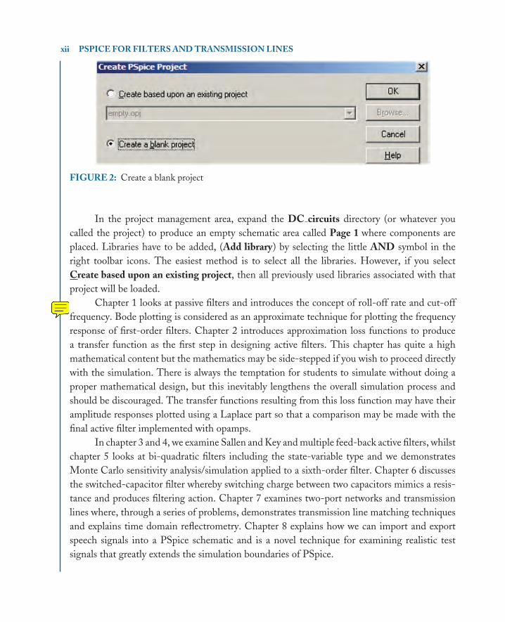
Enter a suitable name in the Name box and select Analog or Mixed A/D and specify aLocation for the file. Press OK and a further menu will appear so tick Create a blank projectas shown in Figure 2.
FIGURE 1: Creating new project file
MOBK064-FM MOBKXXX-Sample.cls March 27, 2007 15:41
xii PSPICE FOR FILTERS AND TRANSMISSION LINES
FIGURE 2: Create a blank project
In the project management area, expand the DC circuits directory (or whatever youcalled the project) to produce an empty schematic area called Page 1 where components areplaced. Libraries have to be added, (Add library) by selecting the little AND symbol in theright toolbar icons. The easiest method is to select all the libraries. However, if you selectCreate based upon an existing project, then all previously used libraries associated with thatproject will be loaded.
Chapter 1 looks at passive filters and introduces the concept of roll-off rate and cut-offfrequency. Bode plotting is considered as an approximate technique for plotting the frequencyresponse of first-order filters. Chapter 2 introduces approximation loss functions to producea transfer function as the first step in designing active filters. This chapter has quite a highmathematical content but the mathematics may be side-stepped if you wish to proceed directlywith the simulation. There is always the temptation for students to simulate without doing aproper mathematical design, but this inevitably lengthens the overall simulation process andshould be discouraged. The transfer functions resulting from this loss function may have theiramplitude responses plotted using a Laplace part so that a comparison may be made with thefinal active filter implemented with opamps.
In chapter 3 and 4, we examine Sallen and Key and multiple feed-back active filters, whilstchapter 5 looks at bi-quadratic filters including the state-variable type and we demonstratesMonte Carlo sensitivity analysis/simulation applied to a sixth-order filter. Chapter 6 discussesthe switched-capacitor filter whereby switching charge between two capacitors mimics a resis-tance and produces filtering action. Chapter 7 examines two-port networks and transmissionlines where, through a series of problems, demonstrates transmission line matching techniquesand explains time domain reflectrometry. Chapter 8 explains how we can import and exportspeech signals into a PSpice schematic and is a novel technique for examining realistic testsignals that greatly extends the simulation boundaries of PSpice.

MOBK064-FM MOBKXXX-Sample.cls March 27, 2007 15:41
PREFACE xiii
ACKNOWLEDGMENTSAnyone who has written a textbook knows that a successful product relies on lots of peoplenot directly involved. I would like to thank a retired head of our department, Bart O’Connorwhose lectures I had the pleasure of attending all those years ago on transmission line theory.Thanks to my son, Lee Tobin, who wrote a very useful program ‘Wav2ASCII’ for creatingASCII speech files for processing in PSpice and subsequently playing back the processed fileafter simulation. This small program really extends the simulation boundaries of PSpice greatly.Lastly, thanks to Dr Mike Murphy, Director of Engineering, Dublin Institute of Technology(DIT) for his interest and encouragement in my PSpice books.

MOBK064-FM MOBKXXX-Sample.cls March 27, 2007 15:41

book Mobk064 March 27, 2007 15:49
1
C H A P T E R 1
Passive Filters and Bode Plotting
1.1 FILTER TYPESFilters are used to modify the frequency spectrum of signals and the five basic filter types are:
� Low-pass . . . . . . . . . passes low frequencies but attenuates high frequencies,� High-pass . . . . . . . . . passes high frequencies but attenuates low frequencies� Bandpass. . . . . . . . . passes a band of frequencies and attenuates frequencies outside that
band� Bandstop. . . . . . . . . attenuates a band of frequencies but passes all other frequencies
outside this band� All-pass . . . . . . . . . not really a filter but used to modify the phase response
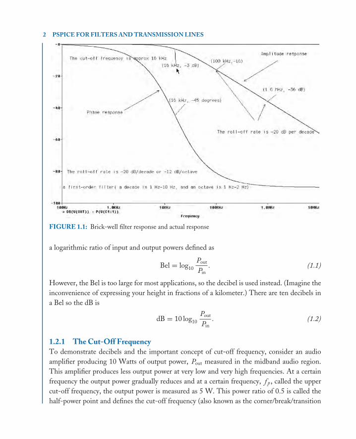
An ideal “brick-wall” low-pass filter response is shown superimposed on a “real” low-passfilter response in Fig. 1.1. What this brick-wall filter does is to pass all frequencies up to acertain frequency called the cut-off frequency ωp , where the subscript stands for passband (alsocalled ωc = 2π fc , the subscript stands for cut-off frequency), and then infinitely attenuate allfrequencies past this value. A real low-pass filter response, however, passes all frequencies withvery little attenuation from DC up to ωp but gradually attenuates signals above this frequency. Ina simple CR low-pass filter response, the signal is gradually attenuated from DC but, because ofthe way capacitive reactance changes with frequency, the attenuation does not become apparentuntil we approach the cut-off frequency. At low frequencies the output signal is in step withthe input signal, i.e., no phase difference between them, but at high frequencies, the outputlags behind the input by ninety degrees, i.e., −90◦, i.e., there is a delay between them.
1.2 DECIBELSThe decibel is the normal unit of measurement in filter design. The logarithmic nature of thehuman ear response thus makes the dB a natural choice for tone control filters such as thebass/treble filters in audio amplifiers. We must consider the Bel as the fundamental unit and is
book Mobk064 March 27, 2007 15:49
2 PSPICE FOR FILTERS AND TRANSMISSION LINES
FIGURE 1.1: Brick-well filter response and actual response
a logarithmic ratio of input and output powers defined as
Bel = log10Pout
Pin. (1.1)
However, the Bel is too large for most applications, so the decibel is used instead. (Imagine theinconvenience of expressing your height in fractions of a kilometer.) There are ten decibels ina Bel so the dB is
dB = 10 log10Pout
Pin. (1.2)
1.2.1 The Cut-Off FrequencyTo demonstrate decibels and the important concept of cut-off frequency, consider an audioamplifier producing 10 Watts of output power, Pout measured in the midband audio region.This amplifier produces less output power at very low and very high frequencies. At a certainfrequency the output power gradually reduces and at a certain frequency, f p , called the uppercut-off frequency, the output power is measured as 5 W. This power ratio of 0.5 is called thehalf-power point and defines the cut-off frequency (also known as the corner/break/transition
book Mobk064 March 27, 2007 15:49
PASSIVE FILTERS AND BODE PLOTTING 3
frequency). The ratio of the power at f p to the power delivered over the passband frequencyrange can be expressed as
dB = 10 log10Pout
Pin= 10 log10
510
= 10 log10 0.5 = −3.01 dB ≈ −3 dB. (1.3)
This particular attenuation is called the passband edge frequency attenuation Amax (ex-plained later). We may express each power component in (1.3) as V2/R, thus the ratio indB is
dB = 10 log10V 2
out/Rout
V 2in/Rin
. (1.4)
Maximum power transfer between a source and a load is desirable in electronic systems [1]. Ex-amples are: a microphone 50 k� source impedance connected to an amplifier input impedanceof 50 k�, a TV whose input impedance of 75 � is connected to a transmission line whosecharacteristic impedance is 75 �, phone handset impedance (300 �) to the transmission linecharacteristic impedance (300 �), etc. In these examples, we see that when the source resistanceis equal to a load resistance, (1.4) is simplified:
dB = 10 log10
(Vout
Vin
)2
= 20 logVout
Vin. (1.5)
A power halving is −3 dB but we wish to see what this is in terms of a voltage ratio.This is calculated by taking the antilog of (1.5) as a log(−3/20) = 0.707 = 1/
√2. The pass-
band region, DC to f p , in a low-pass filter amplitude response, is constant, with little or noattenuation up to the cut-off frequency. When the resistance is equal to the reactance thenthis frequency makes the transfer function Vout/Vin equal to TF = 1/
√2 = 0.707. However,
the passband gain may not always be 1, so care has to be exercised. For example, the passbandgain could be 4, hence the transfer function would be TF = 4/
√2. Note, however, a voltage
doubling in dB is 20 log10 2 = 6 dB.
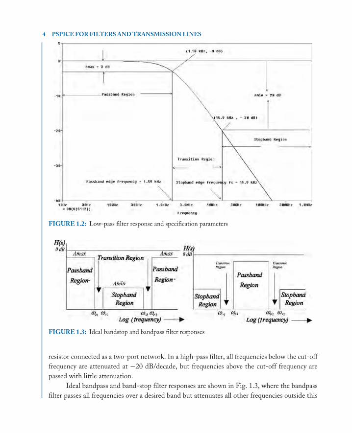
1.2.2 Filter SpecificationA low-pass filter specification includes the passband edge frequency attenuation Amax in dB.This is the attenuation a signal will experience at the passband edge frequency f p , in a simpleCR filter. The attenuation at the stopband edge frequency, fs , is Amin, which, for the first-orderCR filter, is −20 dB. These parameters are all shown on the low-pass filter response shown inFig. 1.2. The parameters are the same for a high-pass filter but a mirror image of the low-passfilter. The transition region between the passband and stopband regions reduces in width whenthe filter order is increased. For example, a first-order filter is achieved using a capacitor and
book Mobk064 March 27, 2007 15:49
4 PSPICE FOR FILTERS AND TRANSMISSION LINES
FIGURE 1.2: Low-pass filter response and specification parameters
FIGURE 1.3: Ideal bandstop and bandpass filter responses
resistor connected as a two-port network. In a high-pass filter, all frequencies below the cut-offfrequency are attenuated at −20 dB/decade, but frequencies above the cut-off frequency arepassed with little attenuation.
Ideal bandpass and band-stop filter responses are shown in Fig. 1.3, where the bandpassfilter passes all frequencies over a desired band but attenuates all other frequencies outside this
book Mobk064 March 27, 2007 15:49
PASSIVE FILTERS AND BODE PLOTTING 5
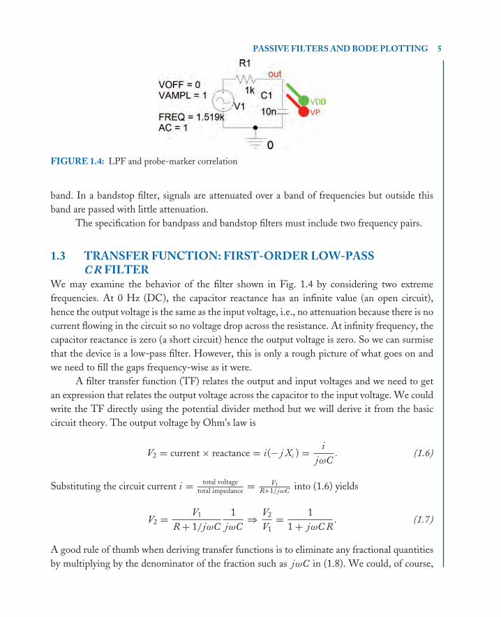
FIGURE 1.4: LPF and probe-marker correlation
band. In a bandstop filter, signals are attenuated over a band of frequencies but outside thisband are passed with little attenuation.
The specification for bandpass and bandstop filters must include two frequency pairs.
1.3 TRANSFER FUNCTION: FIRST-ORDER LOW-PASSC R FILTER
We may examine the behavior of the filter shown in Fig. 1.4 by considering two extremefrequencies. At 0 Hz (DC), the capacitor reactance has an infinite value (an open circuit),hence the output voltage is the same as the input voltage, i.e., no attenuation because there is nocurrent flowing in the circuit so no voltage drop across the resistance. At infinity frequency, thecapacitor reactance is zero (a short circuit) hence the output voltage is zero. So we can surmisethat the device is a low-pass filter. However, this is only a rough picture of what goes on andwe need to fill the gaps frequency-wise as it were.
A filter transfer function (TF) relates the output and input voltages and we need to getan expression that relates the output voltage across the capacitor to the input voltage. We couldwrite the TF directly using the potential divider method but we will derive it from the basiccircuit theory. The output voltage by Ohm’s law is
V2 = current × reactance = i(− j Xc ) = ijωC
. (1.6)
Substituting the circuit current i = total voltagetotal impedance = V1
R+1/jωC into (1.6) yields
V2 = V1
R + 1/jωC1
jωC⇒ V2
V1= 1
1 + jωC R. (1.7)
A good rule of thumb when deriving transfer functions is to eliminate any fractional quantitiesby multiplying by the denominator of the fraction such as jωC in (1.8). We could, of course,

book Mobk064 March 27, 2007 15:49
6 PSPICE FOR FILTERS AND TRANSMISSION LINES
have written this transfer function by applying the voltage divider rule as:
H(s ) = V2
V1= 1/jωC
R + 1/jωC× jωC
jωC= 1
1 + jωC R= 1
1 + j2π f C R= 1
1 + jω/ωp. (1.8)
Here 1/C R is the cut-off frequency ωp . So when ω = ωp the TF = 1/(1 + j1) ⇒ |TF| =1/
√2 = 0.707. A complex number, Z = R + j X, has a magnitude and phase defined as Z =√
R2 + X2∠ tan−1(X/R). Thus, the LPF transfer function 1/(1 + jωC R) has a magnitude1/
√12 + ω2C2 R2, unity gain at DC (the passband region) and the phase response plotted using
θ = − tan−1 ωC R. We already introduced the important concept of cut-off frequency when weconsidered the power relationships in the previous section but another visit should reinforce thisimportant concept. This special frequency occurs where the real part of the transfer functionequals the imaginary part. To obtain an expression for ωp , we equate the TF magnitude to1/
√2 = 0.707. Thus, we may write
|TF| = Vo
Vin= 1√
1 + ω2C2 R2= passband gain√
2= 1√
2⇒
√1 + ω2C2 R2 =
√2. (1.9)
Squaring both sides ω2C2 R2 + 1 = 2 ⇒ ω2C2 R2 = 1 yields the cut-off frequency, in radiansper second, as
ω = 1/C R = ωp . (1.10)
The subscript tells us that at this frequency, the output signal power is reduced by 3 dB (or thevoltage reduced to 0.707 Vin). The cut-off frequency in Hz is ωp/2π , so the cut-off frequencyfor C = 10 nF and R = 10 k� is
f p = 12πC R
= 12π
(10 × 10−9
) (10 × 103
) = 1.59 kHz. (1.11)
1.3.1 Bode PlottingBode plotting (Hendrik Bode—1905–1982) is a useful graphical method for plotting theapproximate filter amplitude and phase responses. We do this by splitting the magnitude ofthe TF into smaller parts containing terms of the form 1 ± jω/ωp and plotting each TF partusing straight-line segments. The complete frequency response is then obtained by adding theindividual responses together. The TF is manipulated into a form (1 ± jω/ωp) by makingthe real part of the complex number one. This is done by dividing every term in the transferfunction by the real part of the complex number. We then get the magnitude of each part of theTF and express it in dB so that we can perform Bode analysis using straight-line or asymptotic
book Mobk064 March 27, 2007 15:49
PASSIVE FILTERS AND BODE PLOTTING 7
FIGURE 1.5: Part (a)
line segments. The transfer function in polar form is
TF = 11 + jω/ωp
= 11 + j f/ f p
⇒ |TF| = 1[1 + ( f/ f p)2]1/2
∠ − tan−1( f/ f p). (1.12)
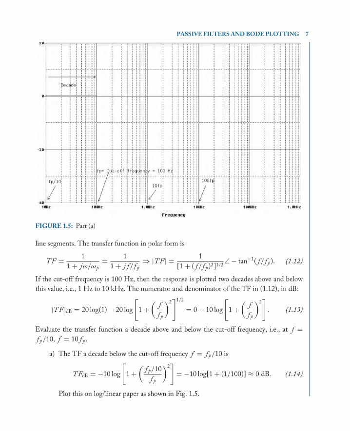
If the cut-off frequency is 100 Hz, then the response is plotted two decades above and belowthis value, i.e., 1 Hz to 10 kHz. The numerator and denominator of the TF in (1.12), in dB:
|TF|dB = 20 log(1) − 20 log
[1 +
(ff p
)2]1/2
= 0 − 10 log
[1 +
(ff p
)2]
. (1.13)
Evaluate the transfer function a decade above and below the cut-off frequency, i.e., at f =f p/10, f = 10 f p .
a) The TF a decade below the cut-off frequency f = f p/10 is
TFdB = −10 log
[1 +
(f p/10
f p
)2]
= −10 log[1 + (1/100)] ≈ 0 dB. (1.14)
Plot this on log/linear paper as shown in Fig. 1.5.
book Mobk064 March 27, 2007 15:49
8 PSPICE FOR FILTERS AND TRANSMISSION LINES
FIGURE 1.6: Part (a) + part (b)
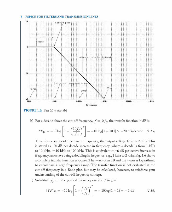
b) For a decade above the cut-off frequency, f =10 f p , the transfer function in dB is
TFdB = −10 log
[1 +
(10 f p
f p
)2]
= −10 log[1 + 100] ≈ −20 dB/decade. (1.15)
Thus, for every decade increase in frequency, the output voltage falls by 20 dB. Thisis stated as –20 dB per decade increase in frequency, where a decade is from 1 kHzto 10 kHz, or 10 kHz to 100 kHz. This is equivalent to –6 dB per octave increase infrequency, an octave being a doubling in frequency, e.g., 1 kHz to 2 kHz. Fig. 1.6 showsa complete transfer function response. The y-axis is in dB and the x-axis is logarithmicto encompass a large frequency range. The transfer function is not evaluated at thecut-off frequency in a Bode plot, but may be calculated, however, to reinforce yourunderstanding of the cut-off frequency concept.
c) Substitute f p into the general frequency variable f to give
|TF|dB = −10 log
[1 +
(f p
f p
)2]
= − 10 log[1 + 1) = − 3 dB. (1.16)

book Mobk064 March 27, 2007 15:49
PASSIVE FILTERS AND BODE PLOTTING 9
FIGURE 1.7: Asymptotic and actual phase response
The complete asymptotic response is obtained by adding the straight-line (Bode)responses together.The filter order (the number of poles—more about this later) determines the roll-offrate in the transition region, i.e., a first-order has a roll-off rate of −20 dB/decade,a second-order is −40 dB/decade, etc. Active filters considered in later chapters haveorders that rarely exceed 10, but digital filters can have very high orders [ref: 2].
1.3.2 Low-Pass CR Filter Phase ResponseWe need to plot the TF phase response as well as the magnitude part using the same Bodetechnique. The phase part of the transfer function is
TF(θ ) = − tan−1( f/ f p). (1.17)
We may plot the approximate phase response by considering the value of the phase a decadeabove and below the cut-off frequency as before, i.e., f = f p/10, and f = 10 f p . For example,
� At f = f p/10, the phase is φ = − tan−1( f p/10 f p) = − tan−1 0.1 ≈ 0◦
� At f = f p , the phase φ = − tan−1 f p/ f p = − tan−1 1 = −45◦
� At f =10 f p , the phase is φ = − tan−1(10 f p/ f p) = − tan−1 10 = −90◦.
The actual and asymptotic phase responses are shown in Fig. 1.7.
book Mobk064 March 27, 2007 15:49
10 PSPICE FOR FILTERS AND TRANSMISSION LINES
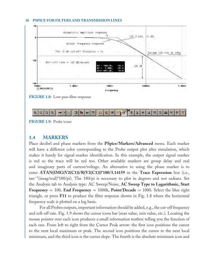
FIGURE 1.8: Low-pass filter response
FIGURE 1.9: Probe icons
1.4 MARKERSPlace decibel and phase markers from the PSpice/Markers/Advanced menu. Each markerwill have a different color corresponding to the Probe output plot after simulation, whichmakes it handy for signal-marker identification. In this example, the output signal markeris red so the trace will be red too. Other available markers are group delay and realand imaginary parts of current/voltage. An alternative to using the phase marker is toenter ATAN(IMG(V2(C1))/R(V2(C1)))*180/3.14159 in the Trace Expression box (i.e.,tan−1(imag/real)*180/pi). The 180/pi is necessary to plot in degrees and not radians. Setthe Analysis tab to Analysis type: AC Sweep/Noise, AC Sweep Type to Logarithmic, StartFrequency = 100, End Frequency = 1000k, Point/Decade = 1000. Select the blue righttriangle, or press F11 to produce the filter response shown in Fig. 1.8 where the horizontalfrequency scale is plotted on a log basis.
For all Probes outputs, important information should be added, e.g., the cut-off frequencyand roll-off rate. Fig. 1.9 shows the cursor icons bar (max value, min value, etc.). Locating themouse pointer over each icon produces a small information textbox telling you the function ofeach one. From left to right from the Cursor Peak arrow: the first icon positions the cursorto the next local maximum or peak. The second icon positions the cursor to the next localminimum, and the third icon is the cursor slope. The fourth is the absolute minimum icon and

book Mobk064 March 27, 2007 15:49
PASSIVE FILTERS AND BODE PLOTTING 11
FIGURE 1.10: “search for min”
the next icon measures the cursor maximum. Pressing will place x and y axis values at thecursor location.
Other icons are: Log x-axis, Fast Fourier Transform FFT, Performance Analysis, Logy-axis, Add Trace, Evaluate Function, and Add Text. The search command (shortcut altTCS) is used to position the cursor at a specific place along a trace. The syntax is: Search[direction] [/start point/] [#consecutive points#] [(range x[,range y])]. Use the F1 button forfurther information on this topic. Turn on the cursor icon and select Trace/Cursor/Searchcommands menu to bring up Fig. 1.10 which shows the search command “search for min”entered in order to move the cursor to the minimum point on the response curve.
The icons at the start are the icons for examining in detail sections of the plot. Press thethird icon from the left and then using the left mouse button expand a section of the plot.
1.4.1 Cut-Off Frequency and Roll-Off RateTwo important things to measure from the frequency response are: (1) The roll-off rate—thisis measured using two cursors separated a decade apart on the linear portion of the response(e.g., 10 kHz to 100 kHz but not on the curved portion of the response). Alternatively, you maymeasure it over an octave (e.g., 2 kHz to 4 kHz). (2) The cut-off frequency—use a single cursorto read the frequency where the output is down by 3 dB from the maximum value (midbandor passband region). The passband gain is generally 0 dB for passive networks, but it may benonzero for active networks which have gain. In that case read the frequency at the point wherethe level is 3 dB below the maximum passband gain.
1.5 ASYMPTOTIC FILTER RESPONSE PLOTTING USING ANFTABLE PART
Fig. 1.11 shows an FTABLE part used to produce a low-pass filter response in Bode asymptoticform, where the cut-off frequency is 1.59 kHz.
Select the FTABLE part and enter the table of values into the columns as shown inFig. 1.12.

book Mobk064 March 27, 2007 15:49
12 PSPICE FOR FILTERS AND TRANSMISSION LINES
FIGURE 1.11: Using the Ftable part to plot a Bode response
FIGURE 1.12: Enter the FTABLE values
From the Analysis Setup, select AC Sweep and then Decade, Point/Decade = 10,001,Start Frequency = 1, and End Frequency = 10 Meg. Press F11 to simulate and plot theasymptotic amplitude response shown in Fig. 1.13.
The Ftable values are entered in magnitude/ phase domain (R I=) or complex numberdomain (R I=YES) form. The values are interpolated and converted to dB, and the phasein degrees. Frequency components outside the table range have zero dB level and imposeupper and lower limits on the output. The DELAY attribute increases the group delay of thefrequency table and is useful if an FTABLE part generates a noncausality warning messageduring a transient analysis. If such is the case, then the delay value is assigned to the DELAYattribute.
1.6 HIGH-PASS CR FILTERThe high-pass filter in Fig. 1.14 has a 1 V input signal applied using a VSIN generator part.Place a Net alias name vout on the output wire segment when selected (or place a Portleft taginstead) and attach voltage markers as shown.
Applying the potential the divider gives the transfer function as
V2
V1= R
R + 1/jωC
/RR
= 11 − j/ωC R
= 11 − j f p/ f
. (1.18)

book Mobk064 March 27, 2007 15:49
PASSIVE FILTERS AND BODE PLOTTING 13
FIGURE 1.13: The FTABLE frequency response
FIGURE 1.14: High-pass CR first-order filter
The cut-off frequency ωp = 1/C R ⇒ f p = 1/2πC R = 1.59 kHz and the magnitude of thetransfer function in dB is
|TF|d B = −10 log[1 + ( f p/ f )2]. (1.19)
At ω = ωp/10, the magnitude of the transfer function is |TF|d B = −10 log[101] ≈ −20dB.Similarly, a decade above the cut-off frequency f = 10 f p makes the transfer function mag-nitude |TF|d B = −10 log[1 + 1/101] ≈ 0 dB. Plot the straight-line approximate amplituderesponse.
1.6.1 Phase Response MeasurementAn expression for the transfer function phase is φ = tan−1( f p/ f ). Remember − tan−1(−x) =tan−1 x. At f = f p/10, the phase angle is φ = tan−1(10 f/ f p) = tan−1 10 = +90◦. At f =f p , the phase is φ = tan−1( f p/ f p) = tan−1 1 = +45◦. At ω = 10ωp , the phase angle is
book Mobk064 March 27, 2007 15:49
14 PSPICE FOR FILTERS AND TRANSMISSION LINES
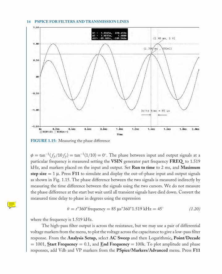
FIGURE 1.15: Measuring the phase difference
φ = tan−1( f p/10 f p) = tan−1(1/10) = 0◦. The phase between input and output signals at aparticular frequency is measured setting the VSIN generator part frequency FREQ to 1.519kHz, and markers placed on the input and output. Set Run to time to 2 ms, and Maximumstep size = 1 µ. Press F11 to simulate and display the out-of-phase input and output signalsas shown in Fig. 1.15. The phase difference between the two signals is measured indirectly bymeasuring the time difference between the signals using the two cursors. We do not measurethe phase difference at the start but wait until all transient signals have died down. Convert themeasured time delay to phase in degrees using the expression
θ = t∗360∗frequency = 85 µs∗360∗1.519 kHz = 45◦ (1.20)
where the frequency is 1.519 kHz.The high-pass filter output is across the resistance, but we may use a pair of differential
voltage markers from the menu, to plot the voltage across the capacitance to give a low-pass filterresponse. From the Analysis Setup, select AC Sweep and then Logarithmic, Point/Decade= 1001, Start Frequency = 0.1, and End Frequency = 100k. To plot amplitude and phaseresponses, add Vdb and VP markers from the PSpice/Markers/Advanced menu. Press F11

book Mobk064 March 27, 2007 15:49
PASSIVE FILTERS AND BODE PLOTTING 15
FIGURE 1.16: Using the measurement menu
FIGURE 1.17: Phase response
to simulate. We will now measure the high pass cut-off frequency using an inbuilt function.Selecting Trace/Evaluate measurement produces the menu shown in Fig. 1.16.
Select Cutoff Highpass 3dB(1) from the right list and substitute the output voltagevariable V(vout) from the left list of variables into the function as shown (i.e., replace 1 withV(vout)) to give an accurate value for the cut-off frequency. Fig. 1.17 shows the phase response
book Mobk064 March 27, 2007 15:49
16 PSPICE FOR FILTERS AND TRANSMISSION LINES
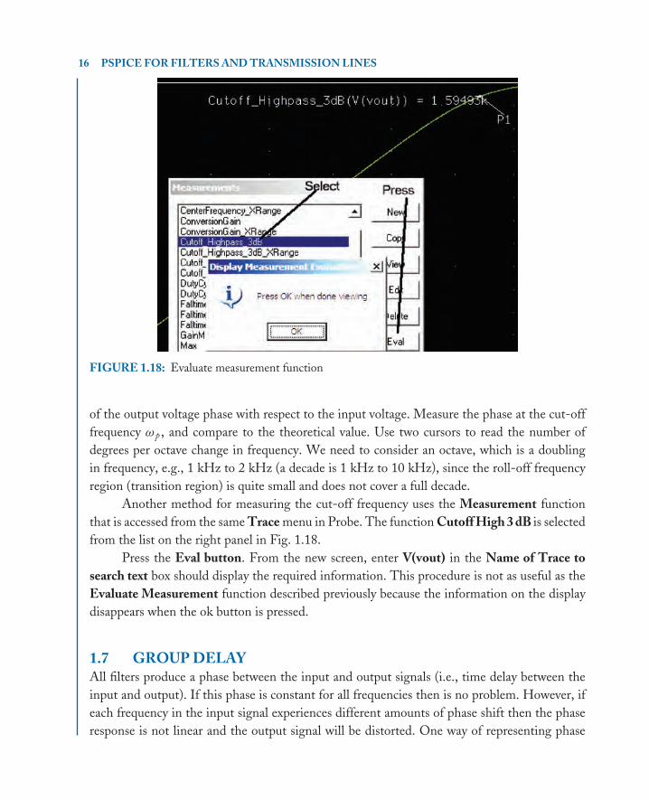
FIGURE 1.18: Evaluate measurement function
of the output voltage phase with respect to the input voltage. Measure the phase at the cut-offfrequency ω p , and compare to the theoretical value. Use two cursors to read the number ofdegrees per octave change in frequency. We need to consider an octave, which is a doublingin frequency, e.g., 1 kHz to 2 kHz (a decade is 1 kHz to 10 kHz), since the roll-off frequencyregion (transition region) is quite small and does not cover a full decade.
Another method for measuring the cut-off frequency uses the Measurement functionthat is accessed from the same Trace menu in Probe. The function Cutoff High 3 dB is selectedfrom the list on the right panel in Fig. 1.18.
Press the Eval button. From the new screen, enter V(vout) in the Name of Trace tosearch text box should display the required information. This procedure is not as useful as theEvaluate Measurement function described previously because the information on the displaydisappears when the ok button is pressed.
1.7 GROUP DELAYAll filters produce a phase between the input and output signals (i.e., time delay between theinput and output). If this phase is constant for all frequencies then is no problem. However, ifeach frequency in the input signal experiences different amounts of phase shift then the phaseresponse is not linear and the output signal will be distorted. One way of representing phase
book Mobk064 March 27, 2007 15:49
PASSIVE FILTERS AND BODE PLOTTING 17
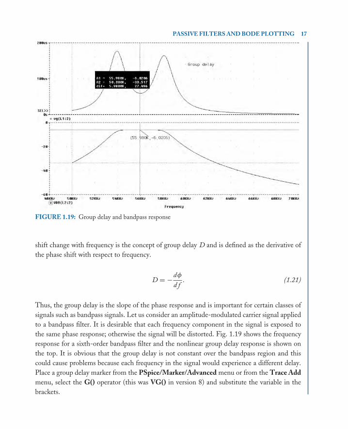
FIGURE 1.19: Group delay and bandpass response
shift change with frequency is the concept of group delay D and is defined as the derivative ofthe phase shift with respect to frequency.
D = −dφ
d f. (1.21)
Thus, the group delay is the slope of the phase response and is important for certain classes ofsignals such as bandpass signals. Let us consider an amplitude-modulated carrier signal appliedto a bandpass filter. It is desirable that each frequency component in the signal is exposed tothe same phase response; otherwise the signal will be distorted. Fig. 1.19 shows the frequencyresponse for a sixth-order bandpass filter and the nonlinear group delay response is shown onthe top. It is obvious that the group delay is not constant over the bandpass region and thiscould cause problems because each frequency in the signal would experience a different delay.Place a group delay marker from the PSpice/Marker/Advanced menu or from the Trace Addmenu, select the G() operator (this was VG() in version 8) and substitute the variable in thebrackets.

book Mobk064 March 27, 2007 15:49
18 PSPICE FOR FILTERS AND TRANSMISSION LINES
FIGURE 1.20: Modified low-pass CR filter
1.8 MODIFIED LOW-PASS FILTERThe modified low-pass filter (MLPF) is used in phase locked loops to provide a constantattenuation at high frequencies, unlike the LPF, which falls off at –20 dB for every decadeincrease in frequency. It also speeds up the response of the PLL compared to an uncompensatedPLL. For the MLPF in Fig. 1.20, obtain:
� The amplitude and phase response,� The two break frequencies,� The constant attenuation factor in dB, and
What is the total phase at the first cut-off frequency?The numerator and denominator of the transfer function are multiplied by jωC:
TF = V 2V 1
= R2 + 1/jωCR1 + R2 + 1/jωC
(jωCjωC
)= 1 + jωC R2
1 + jωC(R1 + R2)= 1 + jω/ωp1
1 + jω/ωp2. (1.22)
The two cut-off frequencies are ωp1 = 1/C R2 rs−1 and ωp2 = 1/C(R1 + R2) rs−1, whereωp1 > ωp2. Express (1.22) in magnitude and phase form as
|TF| =√
1 + (ω/ωp1)2√1 + (ω/ωp2)2
∠[
tan−1(
ω
ωp1
)− tan−1
(ω
ωp2
)]. (1.23)
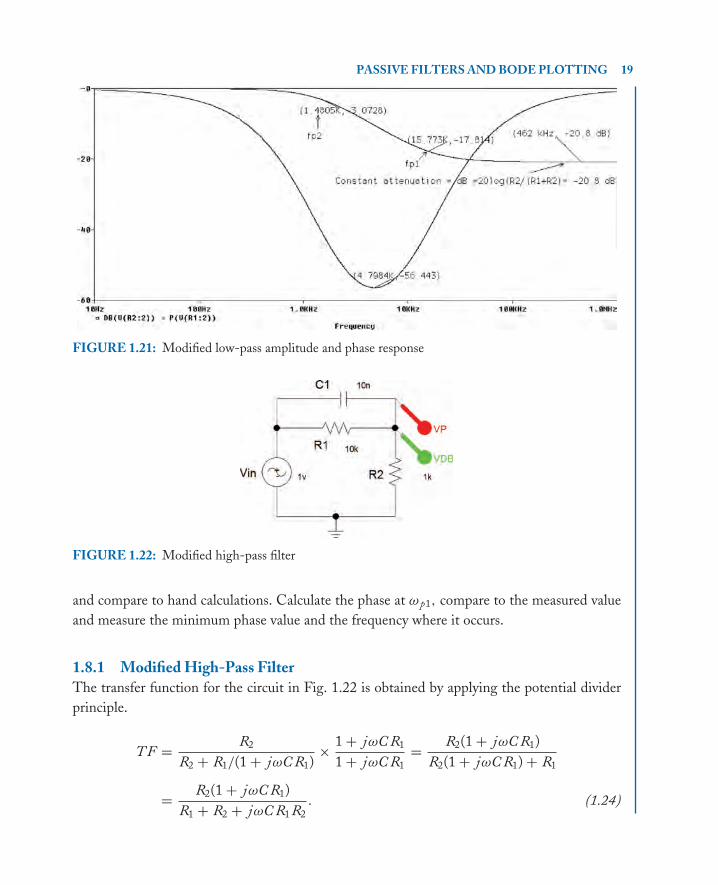
From the Analysis menu, select AC Sweep and Logarithmic, Point/Decade = 1001, StartFrequency = 10, and End Frequency=100 k. Press F11 to simulate and plot the amplitude andphase responses shown in Fig. 1.21. Measure the constant attenuation 20 log[R2/(R1 + R2)]
book Mobk064 March 27, 2007 15:49
PASSIVE FILTERS AND BODE PLOTTING 19
FIGURE 1.21: Modified low-pass amplitude and phase response
FIGURE 1.22: Modified high-pass filter
and compare to hand calculations. Calculate the phase at ω p1, compare to the measured valueand measure the minimum phase value and the frequency where it occurs.
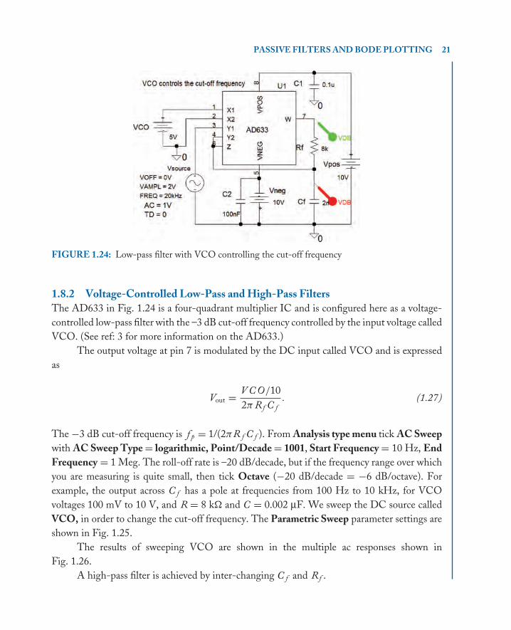
1.8.1 Modified High-Pass FilterThe transfer function for the circuit in Fig. 1.22 is obtained by applying the potential dividerprinciple.
TF = R2
R2 + R1/(1 + jωC R1)× 1 + jωC R1
1 + jωC R1= R2(1 + jωC R1)
R2(1 + jωC R1) + R1
= R2(1 + jωC R1)R1 + R2 + jωC R1 R2
. (1.24)

book Mobk064 March 27, 2007 15:49
20 PSPICE FOR FILTERS AND TRANSMISSION LINES
FIGURE 1.23: Modified high-pass filter phase and amplitude response
Dividing above and below by (R1 + R2) makes the denominator real part one (A require-ment for Bode plotting).
TF =(
R2
R1 + R2
)(1 + jωC R1)
1 + jωC(R2 R1)/(R1 + R2)= R2
R1 + R2
(1 + jω
/ωp1
1 + jω/ωp2
). (1.25)
The cut-off frequencies are: f p1 = 1/2πC R1 Hz and f p2 = 1/2πC(R1 R2)/(R1 + R2)Hz.Thus, the TF has a zero at ω p1 and a pole at ω p2. The transfer function in magnitude andphase is
|TF| = R2
R1 + R2
√1 + (ω/ωp1)2√1 + (ω/ωp2)2
∠[tan−1(ω/ωp1) − tan−1(ω/ωp2)]. (1.26)
The TF magnitude part is expressed in decibels as
|TF| = 20 logR2
R1 + R2+ 10 log
[1 +
(ω
ωp1
)2]
− 10 log
[1 +
(ω
ωp2
)2]
.
From the Analysis Setup, select AC Sweep and Logarithmic, Point/Decade = 1001, StartFrequency = 10, and End Frequency=10meg. Press F11 to simulate and obtain the amplitudeand phase response for the modified high-pass filter (MHPF) as shown in Fig. 1.23.
Measure the constant attenuation factor 20 log(R2/(R1 + R2)) and phase at the cut-frequency ω p1 and compare to the values by a calculator. Measure the maximum phase valueand the frequency where it occurs.
book Mobk064 March 27, 2007 15:49
PASSIVE FILTERS AND BODE PLOTTING 21
FIGURE 1.24: Low-pass filter with VCO controlling the cut-off frequency
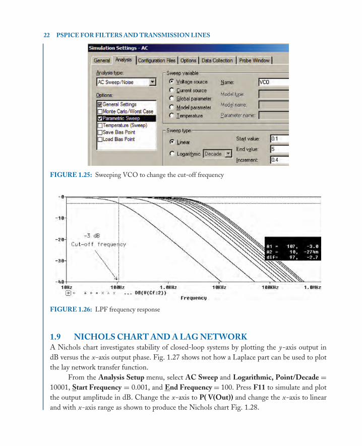
1.8.2 Voltage-Controlled Low-Pass and High-Pass FiltersThe AD633 in Fig. 1.24 is a four-quadrant multiplier IC and is configured here as a voltage-controlled low-pass filter with the –3 dB cut-off frequency controlled by the input voltage calledVCO. (See ref: 3 for more information on the AD633.)
The output voltage at pin 7 is modulated by the DC input called VCO and is expressedas
Vout = V C O/102π Rf C f
. (1.27)
The −3 dB cut-off frequency is f p = 1/(2πR f C f ). From Analysis type menu tick AC Sweepwith AC Sweep Type = logarithmic, Point/Decade = 1001, Start Frequency = 10 Hz, EndFrequency = 1 Meg. The roll-off rate is –20 dB/decade, but if the frequency range over whichyou are measuring is quite small, then tick Octave (−20 dB/decade = −6 dB/octave). Forexample, the output across C f has a pole at frequencies from 100 Hz to 10 kHz, for VCOvoltages 100 mV to 10 V, and R = 8 k� and C = 0.002 µF. We sweep the DC source calledVCO, in order to change the cut-off frequency. The Parametric Sweep parameter settings areshown in Fig. 1.25.
The results of sweeping VCO are shown in the multiple ac responses shown inFig. 1.26.
A high-pass filter is achieved by inter-changing C f and Rf .
book Mobk064 March 27, 2007 15:49
22 PSPICE FOR FILTERS AND TRANSMISSION LINES
FIGURE 1.25: Sweeping VCO to change the cut-off frequency
FIGURE 1.26: LPF frequency response
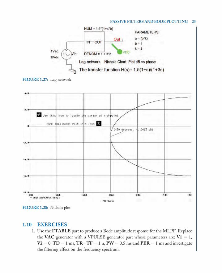
1.9 NICHOLS CHART AND A LAG NETWORKA Nichols chart investigates stability of closed-loop systems by plotting the y-axis output indB versus the x-axis output phase. Fig. 1.27 shows not how a Laplace part can be used to plotthe lay network transfer function.
From the Analysis Setup menu, select AC Sweep and Logarithmic, Point/Decade =10001, Start Frequency = 0.001, and End Frequency = 100. Press F11 to simulate and plotthe output amplitude in dB. Change the x-axis to P( V(Out)) and change the x-axis to linearand with x-axis range as shown to produce the Nichols chart Fig. 1.28.
book Mobk064 March 27, 2007 15:49
PASSIVE FILTERS AND BODE PLOTTING 23
FIGURE 1.27: Lag network
FIGURE 1.28: Nichols plot
1.10 EXERCISES1. Use the FTABLE part to produce a Bode amplitude response for the MLPF. Replace
the VAC generator with a VPULSE generator part whose parameters are: V1 = 1,V2 = 0, TD = 1 ms, TR=TF = 1 n, PW = 0.5 ms and PER = 1 ms and investigatethe filtering effect on the frequency spectrum.
book Mobk064 March 27, 2007 15:49
24 PSPICE FOR FILTERS AND TRANSMISSION LINES
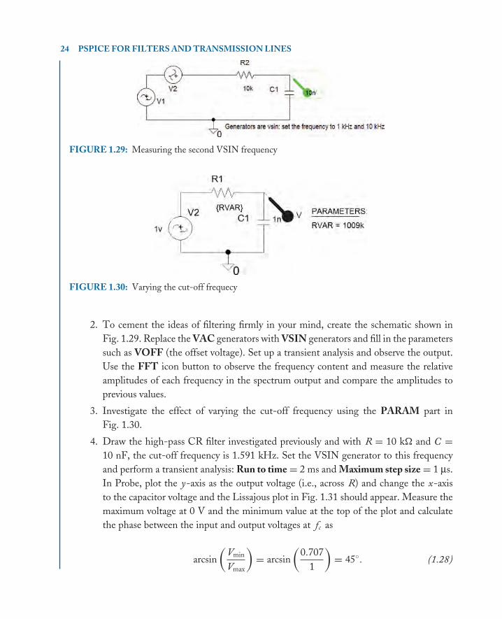
FIGURE 1.29: Measuring the second VSIN frequency
FIGURE 1.30: Varying the cut-off frequecy
2. To cement the ideas of filtering firmly in your mind, create the schematic shown inFig. 1.29. Replace the VAC generators with VSIN generators and fill in the parameterssuch as VOFF (the offset voltage). Set up a transient analysis and observe the output.Use the FFT icon button to observe the frequency content and measure the relativeamplitudes of each frequency in the spectrum output and compare the amplitudes toprevious values.
3. Investigate the effect of varying the cut-off frequency using the PARAM part inFig. 1.30.
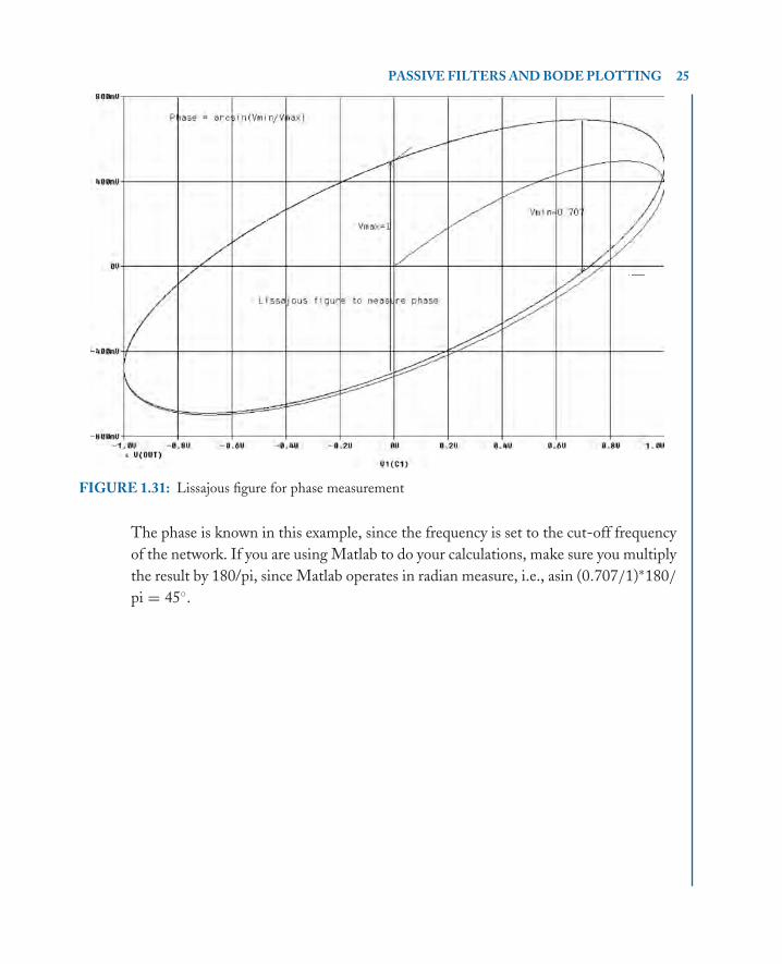
4. Draw the high-pass CR filter investigated previously and with R = 10 k� and C =10 nF, the cut-off frequency is 1.591 kHz. Set the VSIN generator to this frequencyand perform a transient analysis: Run to time = 2 ms and Maximum step size = 1 µs.In Probe, plot the y-axis as the output voltage (i.e., across R) and change the x-axisto the capacitor voltage and the Lissajous plot in Fig. 1.31 should appear. Measure themaximum voltage at 0 V and the minimum value at the top of the plot and calculatethe phase between the input and output voltages at fc as
arcsin(
Vmin
Vmax
)= arcsin
(0.707
1
)= 45◦. (1.28)
book Mobk064 March 27, 2007 15:49
PASSIVE FILTERS AND BODE PLOTTING 25
FIGURE 1.31: Lissajous figure for phase measurement
The phase is known in this example, since the frequency is set to the cut-off frequencyof the network. If you are using Matlab to do your calculations, make sure you multiplythe result by 180/pi, since Matlab operates in radian measure, i.e., asin (0.707/1)∗180/
pi = 45◦.

book Mobk064 March 27, 2007 15:49
book Mobk064 March 27, 2007 15:49
27
C H A P T E R 2
Loss Functions and ActiveFilter Design
2.1 APPROXIMATION LOSS FUNCTIONSActive filters use capacitors, resistors, and op-amps (in general, inductors are not used as theytend to be large at low frequencies and also radiate magnetic fields). They also require DCpower supplies and have a frequency range limited by the quality of the operational amplifierused. To design these filters, we carry out a mathematical analysis that uses approximation lossfunctions A($), which when inverted produce a filter transfer function H($), i.e.,
H($) = 1A($)
. (2.1)
This inversion turns an all-zero function into an all-pole transfer function. Popular approxi-mation loss functions are:
� Bessel,� Butterworth,� Chebychev, and� Elliptical
2.2 BUTTERWORTH APPROXIMATING FUNCTIONA low-pass Butterworth approximation loss function, in magnitude squared form, is
∣∣A( jω)∣∣2 = 1 + ∣∣F( jω)
∣∣2. (2.2)
where the maximally-flat Butterworth characteristic function is defined as∣∣F( jω)
∣∣ = ε(ω/ωp)n. (2.3)
Epsilon is a function that allows Amax to be adjusted to a value less than −3 dB but moreabout that later. Substituting (2.3) into (2.2) yields an expression for the magnitude of the loss

book Mobk064 March 27, 2007 15:49
28 PSPICE FOR FILTERS AND TRANSMISSION LINES
function∣∣A( jω)
∣∣ = [1 + ε2(ω/ωp)2n]1/2
. (2.4)
The loss function attenuation in the passband region 0 < ω < ωp is called Amax and theattenuation in the stopband region ω ≥ ωs is Amin; expressed in dB as
A( jω) = 20 log∣∣A( jω)
∣∣ dB. (2.5)
2.2.1 The Frequency Scaling Factor and Filter OrderTo obtain an expression for the frequency scaling factor ε we must substitute ω = ω p into (2.4).
A(ω)∣∣ω=ωp
= Amax = 10 log10[1 + ε2(ωp/ωp)2n ⇒ Amax
= 10 log10[1 + ε2] ⇒ ε =√
100.1Amax − 1. (2.6)
For example, when Amax is equal to 1 dB, then the frequency correction factor ε is equal to0.508 but when Amax = 3 dB, a popular choice, then ε is 1. The attenuation at the stopbandedge frequency ωs is Amin,
A(ω)∣∣ω=ωs
= Amin = 10 log10[1 + ε2(ωs /ωp)2n] ⇒ 0.1Amin
= log10[1 + ε2(ωs /ωp)2n]. (2.7)
Taking anti-logs of both sides
1 + ε2(ωs /ωp)2n = 100.1Amin ⇒ (ωs /ωp)2n = 100.1Amin − 1ε2
. (2.8)
Or substituting for ε2 = 100.1Amax − 1 from (2.6) yields
(ωs /ωp)2n = 100.1Amin − 1100.1Amax − 1
. (2.9)
This yields an expression for the order of the loss function n by taking logs of both sides of(2.9) as
n =log10
[100.1Amin −1100.1Amax −1
]2 log10(ωs /ωp)
. (2.10)
We then go to the Butterworth loss function tables and select the desired loss function. Wemust invert and denormalize the chosen function to produce the required transfer function andat our required cut-off frequency f p . For example, a first-order normalized Butterworth lossfunction is 1 + $, where $ is the normalized complex frequency variable. Invert and denormalize
book Mobk064 March 27, 2007 15:49
LOSS FUNCTIONS AND ACTIVE FILTER DESIGN 29
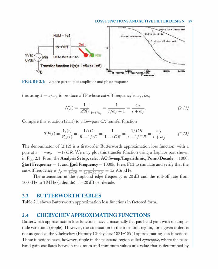
FIGURE 2.1: Laplace part to plot amplitude and phase response
this using $ = s /ωp to produce a TF whose cut-off frequency is ω p , i.e.,
H(s ) = 1A($)
∣∣∣∣$=S/ωp
= 1s /ωp + 1
= ωp
s + ωp. (2.11)
Compare this equation (2.11) to a low-pass CR transfer function
TF(s ) = Vo (s )Vin(s )
= 1/s CR + 1/s C
= 11 + s C R
= 1/C Rs + 1/C R
= ωp
s + ωp. (2.12)
The denominator of (2.12) is a first-order Butterworth approximation loss function, with apole at s = −ωp = −1/C R. We may plot this transfer function using a Laplace part shownin Fig. 2.1. From the Analysis Setup, select AC Sweep/Logarithmic, Point/Decade = 1000,Start Frequency = 1, and End Frequency = 1000k. Press F11 to simulate and verify that thecut-off frequency is f p = 1
2πC R = 12π10×10−9103 = 15.916 kHz.
The attenuation at the stopband edge frequency is 20 dB and the roll-off rate from100 kHz to 1 MHz (a decade) is −20 dB per decade.
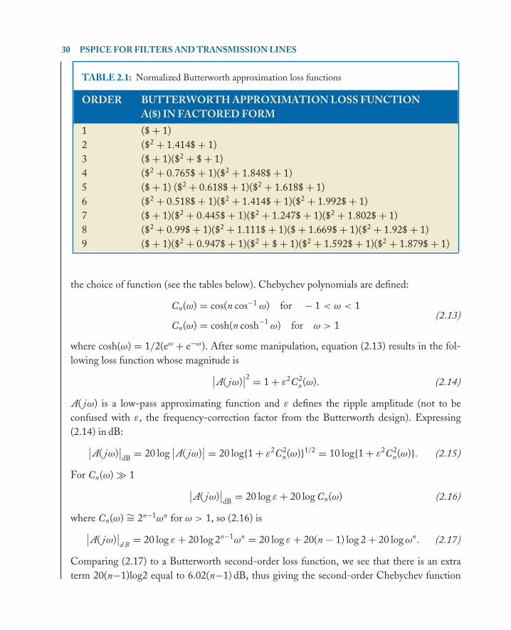
2.3 BUTTERWORTH TABLESTable 2.1 shows Butterworth approximation loss functions in factored form.
2.4 CHEBYCHEV APPROXIMATING FUNCTIONSButterworth approximation loss functions have a maximally flat passband gain with no ampli-tude variations (ripple). However, the attenuation in the transition region, for a given order, isnot as good as the Chebychev (Pafnuty Chebychev 1821–1894) approximating loss functions.These functions have, however, ripple in the passband region called equiripple, where the pass-band gain oscillates between maximum and minimum values at a value that is determined by
book Mobk064 March 27, 2007 15:49
30 PSPICE FOR FILTERS AND TRANSMISSION LINES
TABLE 2.1: Normalized Butterworth approximation loss functions
ORDER BUTTERWORTH APPROXIMATION LOSS FUNCTIONA($) IN FACTORED FORM
1 ($ + 1)2 ($2 + 1.414$ + 1)3 ($ + 1)($2 + $ + 1)4 ($2 + 0.765$ + 1)($2 + 1.848$ + 1)5 ($ + 1) ($2 + 0.618$ + 1)($2 + 1.618$ + 1)6 ($2 + 0.518$ + 1)($2 + 1.414$ + 1)($2 + 1.992$ + 1)7 ($ + 1)($2 + 0.445$ + 1)($2 + 1.247$ + 1)($2 + 1.802$ + 1)8 ($2 + 0.99$ + 1)($2 + 1.111$ + 1)($ + 1.669$ + 1)($2 + 1.92$ + 1)9 ($ + 1)($2 + 0.947$ + 1)($2 + $ + 1)($2 + 1.592$ + 1)($2 + 1.879$ + 1)
the choice of function (see the tables below). Chebychev polynomials are defined:
Cn(ω) = cos(n cos−1 ω) for − 1 < ω < 1
Cn(ω) = cosh(n cosh−1ω) for ω > 1
(2.13)
where cosh(ω) = 1/2(eω + e−ω). After some manipulation, equation (2.13) results in the fol-lowing loss function whose magnitude is
∣∣A( jω)∣∣2 = 1 + ε2C2
n(ω). (2.14)
A( jω) is a low-pass approximating function and ε defines the ripple amplitude (not to beconfused with ε, the frequency-correction factor from the Butterworth design). Expressing(2.14) in dB:
∣∣A( jω)∣∣dB = 20 log
∣∣A( jω)∣∣ = 20 log{1 + ε2C2
n(ω)}1/2 = 10 log{1 + ε2C2n(ω)}. (2.15)
For Cn(ω) � 1∣∣A( jω)
∣∣dB = 20 log ε + 20 log Cn(ω) (2.16)
where Cn(ω) ∼= 2n−1ωn for ω > 1, so (2.16) is∣∣A( jω)
∣∣d B = 20 log ε + 20 log 2n−1ωn = 20 log ε + 20(n − 1) log 2 + 20 log ωn. (2.17)
Comparing (2.17) to a Butterworth second-order loss function, we see that there is an extraterm 20(n−1)log2 equal to 6.02(n−1) dB, thus giving the second-order Chebychev function
book Mobk064 March 27, 2007 15:49
LOSS FUNCTIONS AND ACTIVE FILTER DESIGN 31
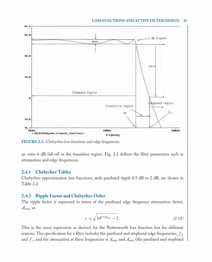
FIGURE 2.2: Chebychev loss functions and edge frequencies
an extra 6 dB fall-off in the transition region. Fig. 2.2 defines the filter parameters such asattenuation and edge frequencies.
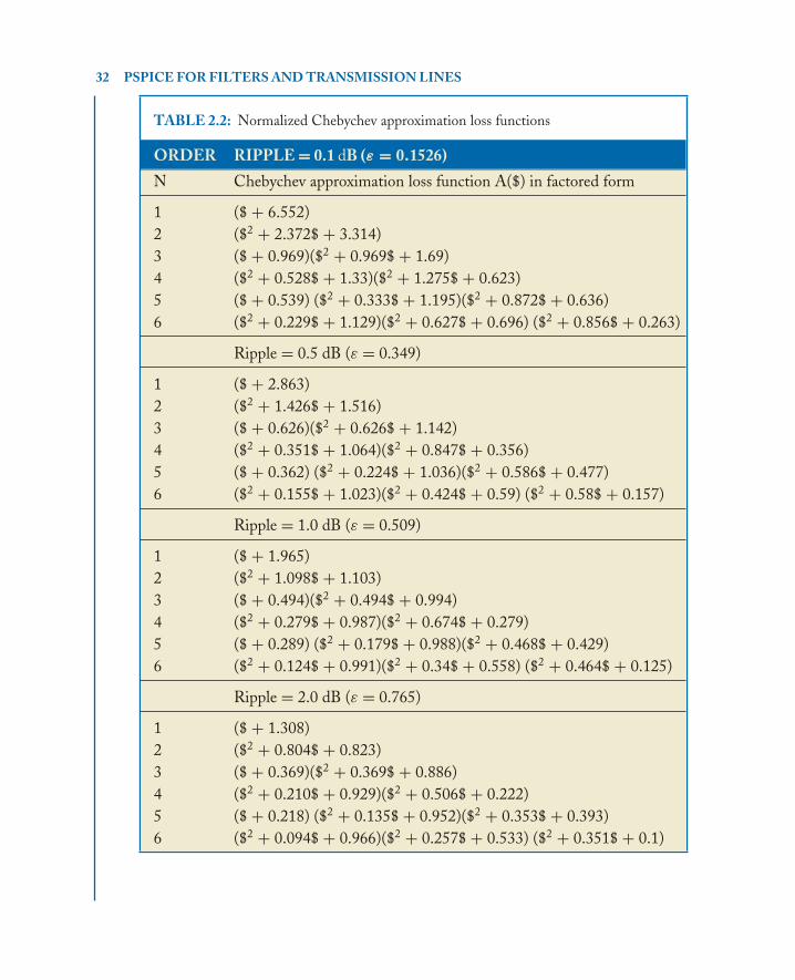
2.4.1 Chebychev TablesChebychev approximation loss functions, with passband ripple 0.5 dB to 2 dB, are shown inTable 2.2.
2.4.2 Ripple Factor and Chebychev OrderThe ripple factor is expressed in terms of the passband edge frequency attenuation factor,Amax, as
ε =√
100.1Amax − 1. (2.18)
This is the same expression as derived for the Butterworth loss function but for differentreasons. The specification for a filter includes the passband and stopband edge frequencies, f p
and f s , and the attenuation at these frequencies is Amax and Amin (the passband and stopband
book Mobk064 March 27, 2007 15:49
32 PSPICE FOR FILTERS AND TRANSMISSION LINES
TABLE 2.2: Normalized Chebychev approximation loss functions
ORDER RIPPLE = 0.1 dB (ε = 0.1526)
N Chebychev approximation loss function A($) in factored form
1 ($ + 6.552)2 ($2 + 2.372$ + 3.314)3 ($ + 0.969)($2 + 0.969$ + 1.69)4 ($2 + 0.528$ + 1.33)($2 + 1.275$ + 0.623)5 ($ + 0.539) ($2 + 0.333$ + 1.195)($2 + 0.872$ + 0.636)6 ($2 + 0.229$ + 1.129)($2 + 0.627$ + 0.696) ($2 + 0.856$ + 0.263)
Ripple = 0.5 dB (ε = 0.349)
1 ($ + 2.863)2 ($2 + 1.426$ + 1.516)3 ($ + 0.626)($2 + 0.626$ + 1.142)4 ($2 + 0.351$ + 1.064)($2 + 0.847$ + 0.356)5 ($ + 0.362) ($2 + 0.224$ + 1.036)($2 + 0.586$ + 0.477)6 ($2 + 0.155$ + 1.023)($2 + 0.424$ + 0.59) ($2 + 0.58$ + 0.157)
Ripple = 1.0 dB (ε = 0.509)
1 ($ + 1.965)2 ($2 + 1.098$ + 1.103)3 ($ + 0.494)($2 + 0.494$ + 0.994)4 ($2 + 0.279$ + 0.987)($2 + 0.674$ + 0.279)5 ($ + 0.289) ($2 + 0.179$ + 0.988)($2 + 0.468$ + 0.429)6 ($2 + 0.124$ + 0.991)($2 + 0.34$ + 0.558) ($2 + 0.464$ + 0.125)
Ripple = 2.0 dB (ε = 0.765)
1 ($ + 1.308)2 ($2 + 0.804$ + 0.823)3 ($ + 0.369)($2 + 0.369$ + 0.886)4 ($2 + 0.210$ + 0.929)($2 + 0.506$ + 0.222)5 ($ + 0.218) ($2 + 0.135$ + 0.952)($2 + 0.353$ + 0.393)6 ($2 + 0.094$ + 0.966)($2 + 0.257$ + 0.533) ($2 + 0.351$ + 0.1)

book Mobk064 March 27, 2007 15:49
LOSS FUNCTIONS AND ACTIVE FILTER DESIGN 33
FIGURE 2.3: Laplace part for plotting transfer functions
attenuation figures respectively). At ω = ωs , the attenuation is
A(ω)∣∣ω=ωs
= Amin = 10 log[1 + ε2C2n(ωs /ωp)] ⇒ 0.1Amin
= log[1 + ε2C2n(ωs /ωp)]. (2.19)
Using this result and the ripple factor, it can be shown that the loss function order is determinedas
n =cosh−1
[100.1Amin −1100.1Amax −1
]1/2
cosh−1(�s ). (2.20)
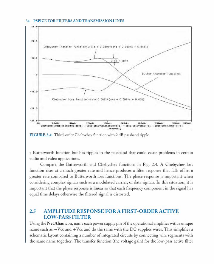
2.4.3 Plotting Chebychev and Butterworth FunctionWe will use Laplace parts in Fig. 2.3 to plot and compare loss and transfer functions. Athird-order Chebychev loss function ($ + 0.369)*($*$ + 0.369*$ + 0.886) is entered in theDENOM of the Laplace part and in the NUM part of a second Laplace part. This will displaya Chebychev loss function and transfer function. Similarly, enter the second-order Butterworthloss function ($*$ + 1.414*$ + 1) in the NUM entry of the last Laplace part.
From the Analysis Setup, select AC Sweep, Logarithmic, Point/Decade = 1001, StartFrequency = 0.01, and End Frequency = 10. Press F11 to simulate. The frequency responseof a Chebychev loss function and its inverse are plotted in Fig. 2.4, and shows a 2 dB ripplein the passband region. A Chebychev transfer function has a steeper roll-off rate compared to
book Mobk064 March 27, 2007 15:49
34 PSPICE FOR FILTERS AND TRANSMISSION LINES
FIGURE 2.4: Third-order Chebychev function with 2 dB passband ripple
a Butterworth function but has ripples in the passband that could cause problems in certainaudio and video applications.
Compare the Butterworth and Chebychev functions in Fig. 2.4. A Chebychev lossfunction rises at a much greater rate and hence produces a filter response that falls off at agreater rate compared to Butterworth loss functions. The phase response is important whenconsidering complex signals such as a modulated carrier, or data signals. In this situation, it isimportant that the phase response is linear so that each frequency component in the signal hasequal time delays otherwise the filtered signal is distorted.
2.5 AMPLITUDE RESPONSE FOR A FIRST-ORDER ACTIVELOW-PASS FILTER
Using the Net Alias icon, name each power supply pin of the operational amplifier with a uniquename such as −Vcc and +Vcc and do the same with the DC supplies wires. This simplifies aschematic layout containing a number of integrated circuits by connecting wire segments withthe same name together. The transfer function (the voltage gain) for the low-pass active filter

book Mobk064 March 27, 2007 15:49
LOSS FUNCTIONS AND ACTIVE FILTER DESIGN 35
FIGURE 2.5: First-order active filter
in Fig. 2.5 is
Av = Vout
Vin= Z2
Z1= R2
1 + jωC R2/R1. (2.21)
The gain in the magnitude form is
|Av| = R2
R1
1[1 + (2π f C R2)2]0.5
= R2
R1
1[1 + (ω/ωp)2]0.5
. (2.22)
The cut-off frequency is ωp = 1/C R2 rs−1. Set Run to time to 2 ms and Maximum step sizeto 400 ns. Press F11 to simulate and display the antiphase input and output signals shown inFig. 2.6.
Change the capacitance to 10 nF and observe the effect on the waveforms.Change the marker to VdB. From the Analysis Setup menu, select AC Sweep/Decade,
Point/Decade = 1001, Start Frequency = 10, and End Frequency = 100k. Simulate withF11 to produce the frequency response for R2 = 10 k� in Fig. 2.7 and resimulate forR2 = 20 k�.
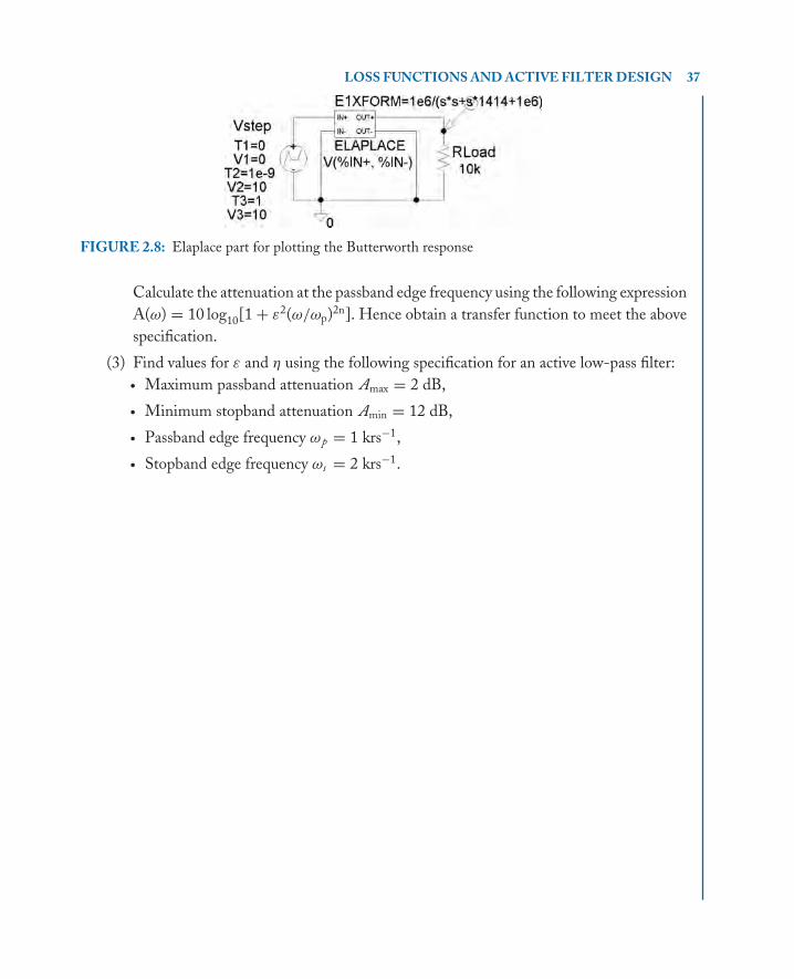
2.6 EXERCISES(1) Investigate the ELAPLACE part for plotting the step response of a second-order
Butterworth transfer function shown in Fig. 2.8. Substitute VAC for VPWL and plotthe frequency response.
book Mobk064 March 27, 2007 15:49
36 PSPICE FOR FILTERS AND TRANSMISSION LINES
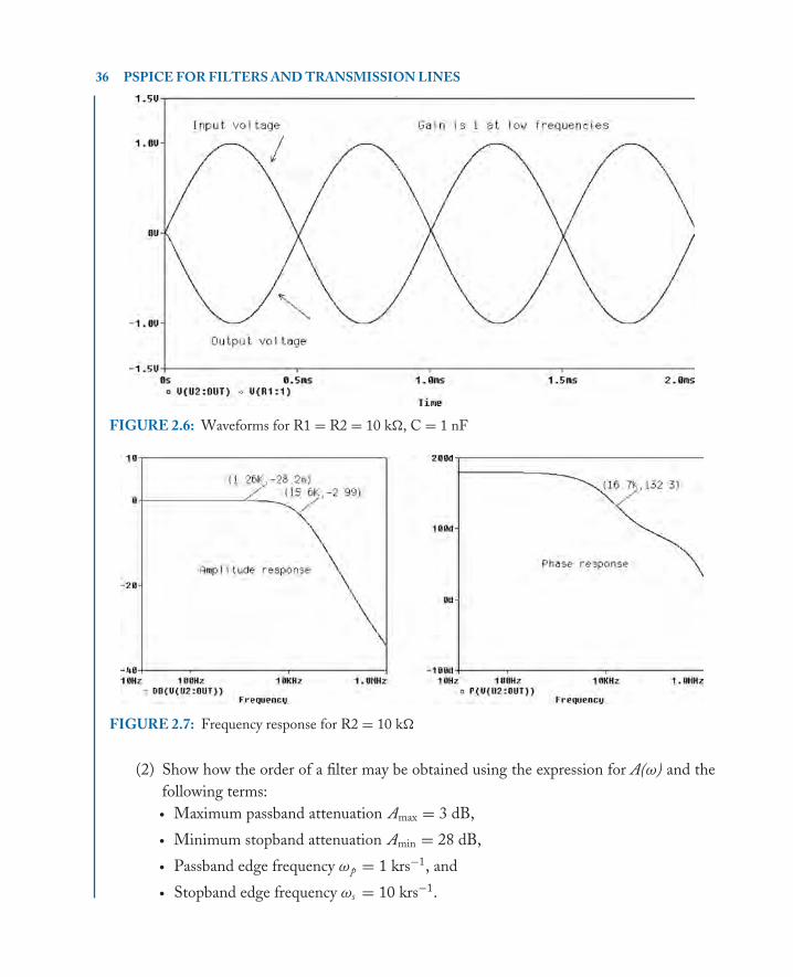
FIGURE 2.6: Waveforms for R1 = R2 = 10 k�, C = 1 nF
FIGURE 2.7: Frequency response for R2 = 10 k�
(2) Show how the order of a filter may be obtained using the expression for A(ω) and thefollowing terms:� Maximum passband attenuation Amax = 3 dB,� Minimum stopband attenuation Amin = 28 dB,� Passband edge frequency ωp = 1 krs−1, and� Stopband edge frequency ωs = 10 krs−1.
book Mobk064 March 27, 2007 15:49
LOSS FUNCTIONS AND ACTIVE FILTER DESIGN 37
FIGURE 2.8: Elaplace part for plotting the Butterworth response
Calculate the attenuation at the passband edge frequency using the following expressionA(ω) = 10 log10[1 + ε2(ω/ωp)2n]. Hence obtain a transfer function to meet the abovespecification.
(3) Find values for ε and η using the following specification for an active low-pass filter:� Maximum passband attenuation Amax = 2 dB,� Minimum stopband attenuation Amin = 12 dB,� Passband edge frequency ωp = 1 krs−1,� Stopband edge frequency ωs = 2 krs−1.

book Mobk064 March 27, 2007 15:49

book Mobk064 March 27, 2007 15:49
39
C H A P T E R 3
Voltage-Controlled Voltage SourceActive Filters
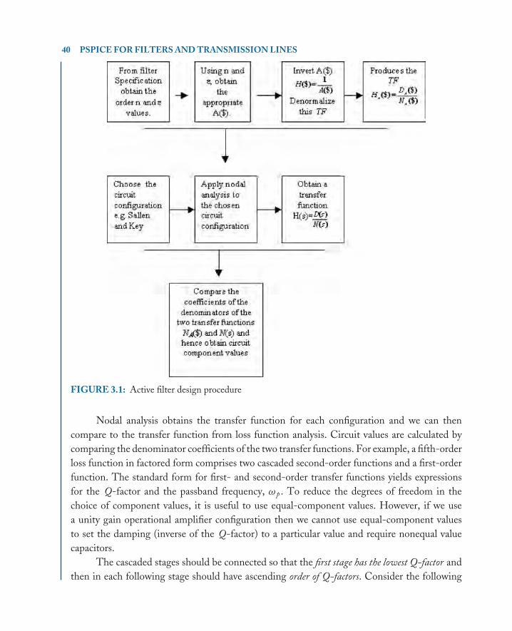
3.1 FILTER TYPESThe procedure for designing active filters to meet a specification is shown in Fig. 3.1. Thefirst four blocks explain how a transfer function is obtained using a specification to select asuitable loss function. The next three blocks show how a second transfer function is obtainedfor a second-order Sallen and Key (or an infinite gain multiple feedback) active filter circuitto implement the first TF derived from loss function analysis. The last block explains howthe comparison between the two transfer function coefficients gives component values for theactive filter.
Many circuit configurations exist for implementing transfer functions from loss functionanalysis. The following circuit configurations are used in the next few chapters:
� Sallen and Key voltage controlled voltage source (VCVS),� Multiple feedback, infinite gain multiple feedback (IGMF),� Biquadratic and state-variable types
We may achieve up to tenth-order filters by cascading first- and second-order types stages.However, identical stages are rarely cascaded as it produces a poor frequency response
at the cut-off frequency as shown in Fig. 3.2. For example, cascading two identical second-order filters produces a fourth-order filter with the attenuation at the cut-off frequency of −6dB, and not −3 dB. A better technique is to design each stage with different Q factors. Wewill investigate voltage-controlled voltage source (VCVS) and infinite gain multiple feedback(IGMF) filter types. These have high input and low output impedances and so may be cascadedwithout any loading problems. We can produce higher-order filters without the need forbuffering between each stage. These two types have high Q-factor sensitivities which is ameasure of the effect on the response when circuit component values deviate from their statedmanufactured value. This is called tolerance and is investigated using the Monte Carlo/Worstcase facility in Probe.
book Mobk064 March 27, 2007 15:49
40 PSPICE FOR FILTERS AND TRANSMISSION LINES
FIGURE 3.1: Active filter design procedure
Nodal analysis obtains the transfer function for each configuration and we can thencompare to the transfer function from loss function analysis. Circuit values are calculated bycomparing the denominator coefficients of the two transfer functions. For example, a fifth-orderloss function in factored form comprises two cascaded second-order functions and a first-orderfunction. The standard form for first- and second-order transfer functions yields expressionsfor the Q-factor and the passband frequency, ω p . To reduce the degrees of freedom in thechoice of component values, it is useful to use equal-component values. However, if we usea unity gain operational amplifier configuration then we cannot use equal-component valuesto set the damping (inverse of the Q-factor) to a particular value and require nonequal valuecapacitors.
The cascaded stages should be connected so that the first stage has the lowest Q-factor andthen in each following stage should have ascending order of Q-factors. Consider the following
book Mobk064 March 27, 2007 15:49
VOLTAGE-CONTROLLED VOLTAGE SOURCE ACTIVE FILTERS 41
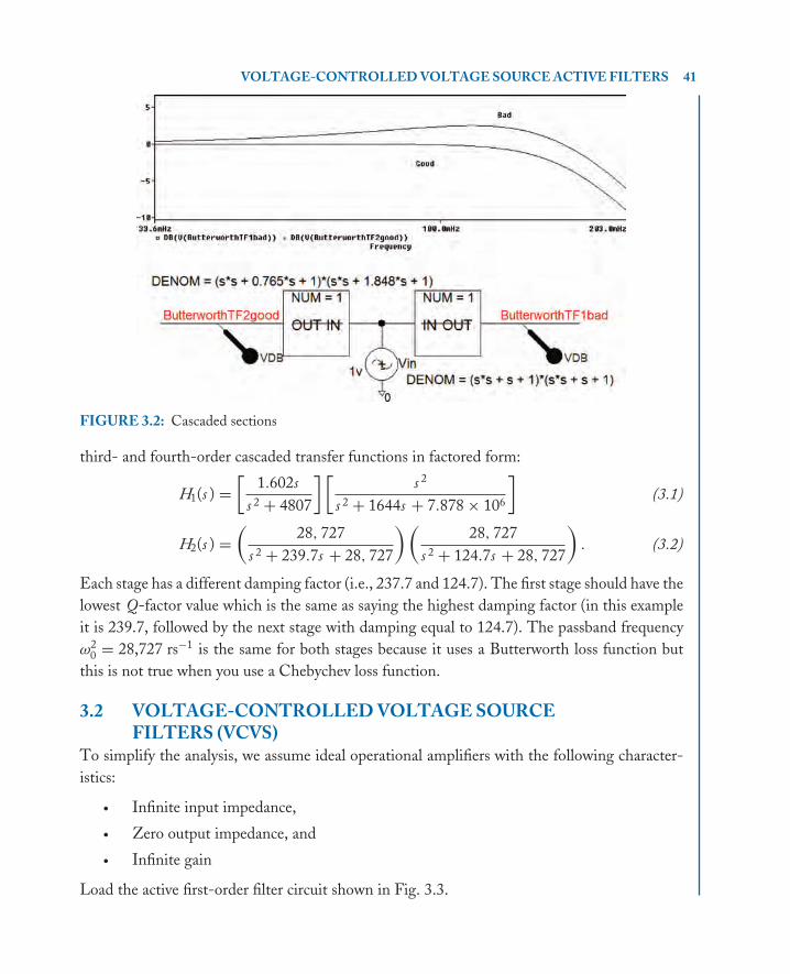
FIGURE 3.2: Cascaded sections
third- and fourth-order cascaded transfer functions in factored form:
H1(s ) =[
1.602ss 2 + 4807
] [s 2
s 2 + 1644s + 7.878 × 10⁶
](3.1)
H2(s ) =(
28, 727s 2 + 239.7s + 28, 727
) (28, 727
s 2 + 124.7s + 28, 727
). (3.2)
Each stage has a different damping factor (i.e., 237.7 and 124.7). The first stage should have thelowest Q-factor value which is the same as saying the highest damping factor (in this exampleit is 239.7, followed by the next stage with damping equal to 124.7). The passband frequencyω2
0 = 28,727 rs−1 is the same for both stages because it uses a Butterworth loss function butthis is not true when you use a Chebychev loss function.
3.2 VOLTAGE-CONTROLLED VOLTAGE SOURCEFILTERS (VCVS)
To simplify the analysis, we assume ideal operational amplifiers with the following character-istics:
� Infinite input impedance,� Zero output impedance, and� Infinite gain
Load the active first-order filter circuit shown in Fig. 3.3.
book Mobk064 March 27, 2007 15:49
42 PSPICE FOR FILTERS AND TRANSMISSION LINES
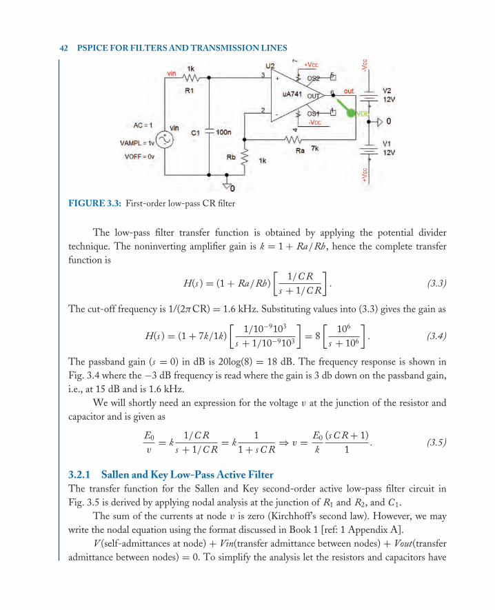
FIGURE 3.3: First-order low-pass CR filter
The low-pass filter transfer function is obtained by applying the potential dividertechnique. The noninverting amplifier gain is k = 1 + Ra/Rb, hence the complete transferfunction is
H(s ) = (1 + Ra/Rb)[
1/C Rs + 1/C R
]. (3.3)
The cut-off frequency is 1/(2πCR) = 1.6 kHz. Substituting values into (3.3) gives the gain as
H(s ) = (1 + 7k/1k)[
1/10−9103
s + 1/10−9103
]= 8
[106
s + 106
]. (3.4)
The passband gain (s = 0) in dB is 20log(8) = 18 dB. The frequency response is shown inFig. 3.4 where the −3 dB frequency is read where the gain is 3 db down on the passband gain,i.e., at 15 dB and is 1.6 kHz.
We will shortly need an expression for the voltage v at the junction of the resistor andcapacitor and is given as
E0
v= k
1/C Rs + 1/C R
= k1
1 + s C R⇒ v = E0
k(s C R + 1)
1. (3.5)
3.2.1 Sallen and Key Low-Pass Active FilterThe transfer function for the Sallen and Key second-order active low-pass filter circuit inFig. 3.5 is derived by applying nodal analysis at the junction of R1 and R2, and C1.
The sum of the currents at node v is zero (Kirchhoff’s second law). However, we maywrite the nodal equation using the format discussed in Book 1 [ref: 1 Appendix A].
V (self-admittances at node) + Vin(transfer admittance between nodes) + Vout(transferadmittance between nodes) = 0. To simplify the analysis let the resistors and capacitors have

book Mobk064 March 27, 2007 15:49
VOLTAGE-CONTROLLED VOLTAGE SOURCE ACTIVE FILTERS 43
FIGURE 3.4: Amplitude response
FIGURE 3.5: Sallen and Key active second-order LPF
equal values so:
v
[1R
+ 1R
+ s C]
− Ei
R− E0
k R− s C E0 = 0. (3.6)
Substitute for v from (3.5) into (3.6) and rearrange
E0(1 + s C R)
k
[2R
+ s C]
− Ei
R− E0
k R− s C E0 = 0. (3.7)
book Mobk064 March 27, 2007 15:49
44 PSPICE FOR FILTERS AND TRANSMISSION LINES
Divide across by E0
(1 + s C R)k
[2R
+ s C]
− Ei
E0 R− 1
k R− s C = 0. (3.8)
Multiply by kR
Ei
E0k = (1 + s C R)(1 + s C R) − 1 − s C Rk = 1 + 3s C R + 1
+ s 2C2 R2 − 1 − s C Rk. (3.9)
Invert (3.9)
E0
Ei= k
s 2C2 R2 + s (3C R − C Rk) + 1. (3.10)
Dividing above and below by the coefficient of s 2, i.e., C2R2 yields
E0
Ei= k 1
C2 R2
s 2 + s (3−k)C R + 1
C2 R2
. (3.11)
Equating the denominator coefficients to the standard form yields
ω0 = 1C R
(3.12)
ω0
Q= (3 − k)
C R⇒ Q = 1
3 − k. (3.13)
The passband gain is obtained by letting all s terms = 0, i.e., G(0) = k.
3.2.2 ExampleAn active low-pass filter is required to meet the following specification:
� The maximum passband loss Amax = 0.5 dB� The minimum stopband loss Amin = 12 dB� The passband edge frequency ωp = 100 rs−1( f p = ωp/2π = 15.9 Hz)� The stopband edge frequency ωs = 400 rs−1
Obtain a Butterworth transfer function and components for a Sallen and Key active filter circuitto meet the above specification. The filter order is calculated as
n =log10
[100.1Amin −1100.1Amax −1
]2 log10(ωs /ωp)
=log10
[100.1×12−1100.1×0.5−1
]2 log10(400/100)
= 1.7 ≈ 2. (3.14)
book Mobk064 March 27, 2007 15:49
VOLTAGE-CONTROLLED VOLTAGE SOURCE ACTIVE FILTERS 45
There are two zeros in a second-order loss function with an angle between them equal to360/2n = 90◦, hence the angle from the real axis and the first zero is 45◦, so the first zero is
s 1 = cos 135 + j sin 135 = −0.707 + j0.707. (3.15)
The second zero is
s 2 = −0.707 − j0.707. (3.16)
The required loss function is thus
A($) = ($ − s 1)($ − s 2) = [$ − (−0.707 + j0.707)][$ − (−0.707 − j0.707)] (3.17)
A($) = ($ + 0.707 + j0.707)($ + 0.707 − j0.707) = $2 + 1.414$ + 1. (3.18)
Denormalize the loss function by replacing $ with s ε1/n/ωp , where the frequency-correctionfactor is ε =
√(100.1.Amax − 1) =
√(100.1×0.5 − 1) = 0.35, so $ is
$ = s0.351/2
100= s
0.59100
. (3.19)
Substitute (3.19) into the second-order inverted loss function to denormalize it:
H(s ) = 1(s 0.59
100
)2+ 1.414
(s 0.59
100
)+ 1
) = 10000s 20.592 + 141.4 × 0.59s + 10000
= 28727s 2 + 239.7s + 28727
. (3.20)
Compare the coefficients of (3.20) to the standard second-order form:
E0
Ei= kω2
p
s 2 + s ω/Q + ω2p
= k/C2 R2
s 2 + s (3 − k)/C R + 1/C2 R2= k∗28727
s 2 + 239.7s + 28727. (3.21)
We have included a gain k to make the passband gain the same in both transfer functions. LetR = 10 k�.
ω2c = 28727 = 1/(C R)2 ⇒ ωc = 169.5 r s −1. (3.22)
This ωc is not the same as ωp from the specification, so we introduce a frequency correctionfactor, ε (required when Amax is less than 3 dB). This factor shifts the passband edge frequency,ωp = 100 rs−1, up to the new cut-off frequency ωc = 169.5 rs−1 ( f c = ωc /2π = 26.97 Hz).At this frequency the attenuation is 3 dB down on the passband gain. (The attenuation atω p = 100 rs−1 is 0.5 dB.) The passband gain k = 20 log(1 + Ra/Rb) = 4 dB, so the gain atω p is (4 − 0.5) dB = 3.5 dB, and at ωc , the gain (4 − 3) = 1 dB. Let R =10 k� to yield
book Mobk064 March 27, 2007 15:49
46 PSPICE FOR FILTERS AND TRANSMISSION LINES
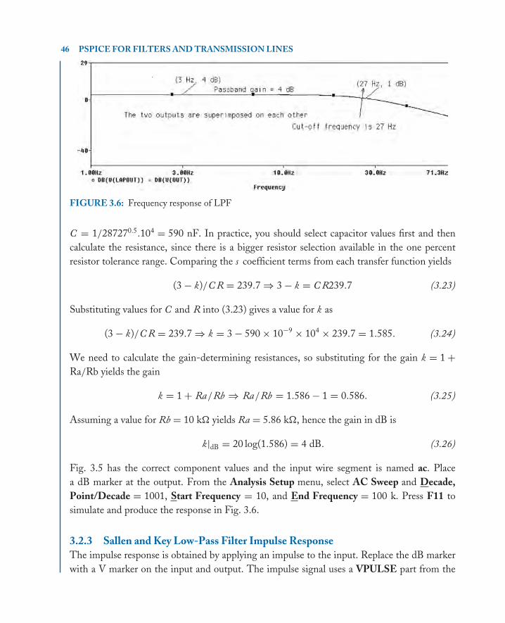
FIGURE 3.6: Frequency response of LPF
C = 1/287270.5.104 = 590 nF. In practice, you should select capacitor values first and thencalculate the resistance, since there is a bigger resistor selection available in the one percentresistor tolerance range. Comparing the s coefficient terms from each transfer function yields
(3 − k)/C R = 239.7 ⇒ 3 − k = C R239.7 (3.23)
Substituting values for C and R into (3.23) gives a value for k as
(3 − k)/C R = 239.7 ⇒ k = 3 − 590 × 10−9 × 104 × 239.7 = 1.585. (3.24)
We need to calculate the gain-determining resistances, so substituting for the gain k = 1 +Ra/Rb yields the gain
k = 1 + Ra/Rb ⇒ Ra/Rb = 1.586 − 1 = 0.586. (3.25)
Assuming a value for Rb = 10 k� yields Ra = 5.86 k�, hence the gain in dB is
k|dB = 20 log(1.586) = 4 dB. (3.26)
Fig. 3.5 has the correct component values and the input wire segment is named ac. Placea dB marker at the output. From the Analysis Setup menu, select AC Sweep and Decade,Point/Decade = 1001, Start Frequency = 10, and End Frequency = 100 k. Press F11 tosimulate and produce the response in Fig. 3.6.
3.2.3 Sallen and Key Low-Pass Filter Impulse ResponseThe impulse response is obtained by applying an impulse to the input. Replace the dB markerwith a V marker on the input and output. The impulse signal uses a VPULSE part from the

book Mobk064 March 27, 2007 15:49
VOLTAGE-CONTROLLED VOLTAGE SOURCE ACTIVE FILTERS 47
FIGURE 3.7: The input impulse function
source library with parameters:
� DC = 0 (offset)� AC = 1 (amplitude)� V1 = 0 (space value)� V2 = 1 (mark value)� TD = 0 s (delay)� TR = 1 µs (rise time)� TF = 1 µs (Fall time)� PW = 10 µs (pulse width----make it short to mimic an ideal impulse)� PER = 1 s (period-----make it very large to create the illusion of only one impulse)
Change Ra to 19 k� to decrease the damping and observe the decaying oscillatory output.The transient setup parameters are: Output File Options/Print values in the output file = 20ns, Run to time = 0.05 s and Maximum step size = 1 µs. Press F11 to produce the impulsein Fig. 3.7.
The impulse spectrum is obtained by selecting the FFT icon. The impulse spectrum is asinc-shaped function sinx/x but PSpice displays absolute values only. Measure the frequency atthe minimum points and determine the relationship between this frequency and the pulse width.You may display both the pulse and its spectrum (time and frequency domain) simultaneously,by selecting Plot/Unsynchronize X-Axis from the Probe screen. Separate the two displayed
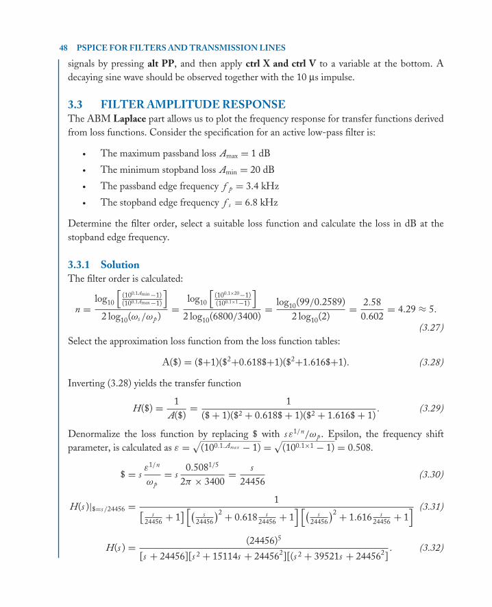
book Mobk064 March 27, 2007 15:49
48 PSPICE FOR FILTERS AND TRANSMISSION LINES
signals by pressing alt PP, and then apply ctrl X and ctrl V to a variable at the bottom. Adecaying sine wave should be observed together with the 10 µs impulse.
3.3 FILTER AMPLITUDE RESPONSEThe ABM Laplace part allows us to plot the frequency response for transfer functions derivedfrom loss functions. Consider the specification for an active low-pass filter is:
� The maximum passband loss Amax = 1 dB� The minimum stopband loss Amin = 20 dB� The passband edge frequency f p = 3.4 kHz� The stopband edge frequency f s = 6.8 kHz
Determine the filter order, select a suitable loss function and calculate the loss in dB at thestopband edge frequency.
3.3.1 SolutionThe filter order is calculated:
n =log10
[(100.1Amin −1)(100.1Amax −1)
]2 log10(ωs /ωp)
=log10
[(100.1×20−1)(100.1×1−1)
]2 log10(6800/3400)
= log10(99/0.2589)2 log10(2)
= 2.580.602
= 4.29 ≈ 5.
(3.27)Select the approximation loss function from the loss function tables:
A($) = ($+1)($2+0.618$+1)($2+1.616$+1). (3.28)
Inverting (3.28) yields the transfer function
H($) = 1A($)
= 1($ + 1)($2 + 0.618$ + 1)($2 + 1.616$ + 1)
. (3.29)
Denormalize the loss function by replacing $ with s ε1/n/ωp . Epsilon, the frequency shiftparameter, is calculated as ε =
√(100.1.Amax − 1) =
√(100.1×1 − 1) = 0.508.
$ = sε1/n
ωp= s
0.5081/5
2π × 3400= s
24456(3.30)
H(s )|$=s /24456 = 1[ s24456 + 1
] [( s24456
)2 + 0.618 s24456 + 1
] [( s24456
)2 + 1.616 s24456 + 1
] (3.31)
H(s ) = (24456)5
[s + 24456][s 2 + 15114s + 244562][(s 2 + 39521s + 244562]. (3.32)

book Mobk064 March 27, 2007 15:49
VOLTAGE-CONTROLLED VOLTAGE SOURCE ACTIVE FILTERS 49
FIGURE 3.8: The ABM Laplace part
Select the Laplace part and enter 8.7484e21 in the NUMerator and enter the denominator inthe DENOM box.
H(s ) = 8.7484e21(s + 24456)∗(s ∗s + 15114∗s + 24456∗∗2)∗(s ∗s + 39530∗s + 24456∗∗2)
. (3.33)
Figure 3.8 shows the transfer function in the ABM Laplace part with the output wire segmentcalled vout and with a dB marker attached. To square a function, enter s *s , or s **2 but youmay also use PWRS(s, 2) as an alternative. This is useful when large powers of s are involved,i.e., PWRS(s, 6) for s 6.
Always use round brackets (square brackets are not allowed) to ensure that the totaldenominator is divided into the numerator. Be careful about multiplication and always use *between brackets, variables and numbers, e.g., (s + 2)∗(s + 1), and 15.91e3*s . The attenuationat the stopband edge frequency is
A(s ) = 10 log10
[1 + ε2
(ω
ωp
)2n]
. (3.34)
The attenuation for n = 5
A(s ) = 10 log10[1 + 0.259(2)10] = 24.5 dB. (3.35)
We must express the transfer function in factored form because we wish to implement eachfactor using individually designed stages. From the Analysis Setup, select AC Sweep, andLogarithmic, Point/Decade = 1001, Start Frequency = 10, and End Frequency = 100k.Press F11 to simulate and plot the fifth-order Butterworth transfer function amplitude response

book Mobk064 March 27, 2007 15:49
50 PSPICE FOR FILTERS AND TRANSMISSION LINES
FIGURE 3.9: Amplitude response
as shown in Fig. 3.9. You may use the Evaluate Measurement Function to check if thespecification is met.
3.4 BUTTERWORTH THIRD ORDER ACTIVEHIGH-PASS FILTER
Obtain a Butterworth high-pass transfer function to meet the following specification:
� The maximum passband loss Amax = 3 dB� The minimum stopband loss Amin = 28 dB� The passband edge frequency ω p = 6000 rs−1
� The stopband edge frequency ωs = 2000 rs−1
Calculate component values for the third-order active filter circuit in Fig. 3.10 to implementthis transfer function.
Let R = 20 k�. The frequency correction factor is one since Amax is −3 dB, or calculatedas
ε =√
(100.1×Amax − 1) =√
(100.1×3 − 1) = 0.9976 ≈ 1. (3.36)
The filter order is calculated as
n =log10
[(100.1Amin −1)(100.1Amax −1)
2 log10(ωs /ωp)=
log10
[(100.1×28−1)(100.1×3−1)
2 log10(6000/2000)= 2.93 ≈ 3. (3.37)