QM/MM Calculations and Applications to Biophysics

QM/MM Calculations and Applications to Biophysics

Marcus Elstner

Physical and Theoretical Chemistry, Technical University of Braunschweig

Proteins, DNA, lipidsProteins, DNA, lipids

N

Computational challengeComputational challenge

~ 1.000-10.000 atoms in protein

~ ns molecular dynamics simulation

(MD, umbrella sampling)

- chemical reactions: proton transfer

- treatment of excited states

QM

Computational problem I: number of atomsComputational problem I: number of atoms

chemical reaction which needs QM treatment

immediate environment: electrostatic and steric interactions

solution, membrane: polarization and structural effects on protein and reaction!

10.000... - several 100.000 atoms

Computational problem II: sampling with MDComputational problem II: sampling with MD

flexibility: not one global minimum

conformational entropy

solvent relaxation

ps – ns timescale (timestep ~ 1fs)

(folding anyway out of reach!)

Optimal setupOptimal setup

ProteinMembrane: = 10 Membrane: = 10

active

Water: = 80

Water: = 80

= 20

= 20

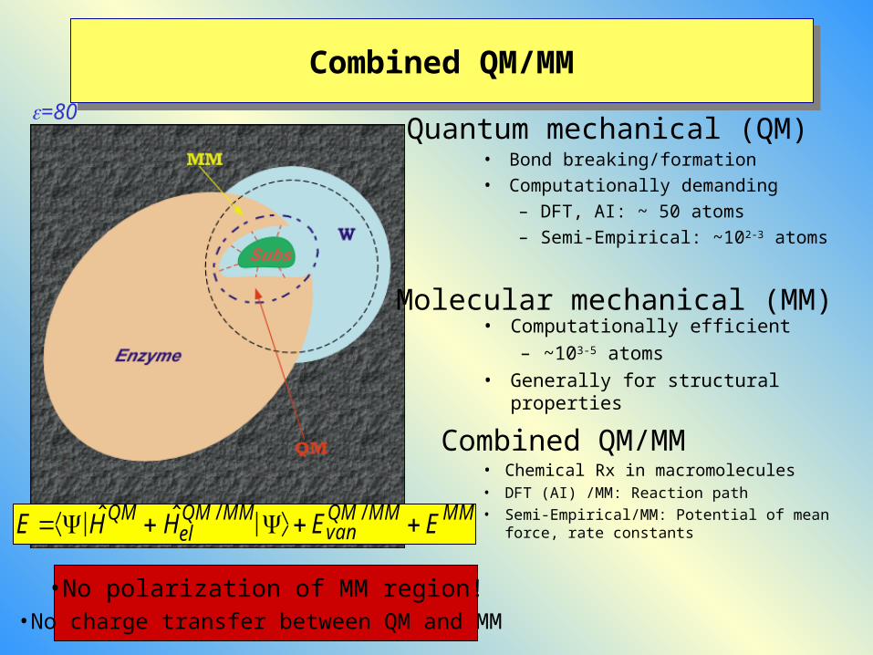
Combined QM/MMCombined QM/MM

=80

• Computationally efficient

– ~103-5 atoms

• Generally for structural properties

• Bond breaking/formation

• Computationally demanding

– DFT, AI: ~ 50 atoms

– Semi-Empirical: ~102-3 atoms

Quantum mechanical (QM)

Molecular mechanical (MM)

Combined QM/MM• Chemical Rx in macromolecules• DFT (AI) /MM: Reaction path • Semi-Empirical/MM: Potential of mean

force, rate constants

E ˆ H QM ˆ H elQM / MM Evan

QM / MM E MM

•No polarization of MM region!•No charge transfer between QM and MM

Combined QM/MMCombined QM/MM

1976 Warshel and Levitt

1986 Singh and Kollman

1990 Field, Bash and KarplusQM • Semi-empirical• quantum chemistry packages: DFT, HF, MP2, LMP2• DFT plane wave codes: CPMD

MM• CHARMM, AMBER, GROMOS, SIGMA,TINKER, ...

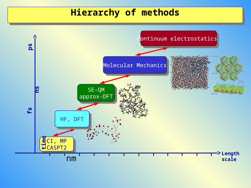
Hierarchy of methodsHierarchy of methods

CI, MPCASPT2

CI, MPCASPT2

Length scale

Continuum electrostatics Continuum electrostatics

Molecular MechanicsMolecular Mechanics

f

s

ps

ns

t i

me

SE-QMapprox-DFT

SE-QMapprox-DFT

HF, DFTHF, DFT

nm

Empirical Force Fields: Molecular Mechanics MM

Empirical Force Fields: Molecular Mechanics MM

models protein + DNA structures quite well

Problem:

- polarization

- charge transfer

- not reactiv in general

ji

ij

ji

ji

ji

ji

ji

ji

ji

dihedrals

N

n impropers

n

bonds anglesb

Dr

qq

rr

knkkbbkV

,,

6

,

,

12

,

,

,

1

2

0

)(2

0

2

0

4

(cos1

kb

k

k

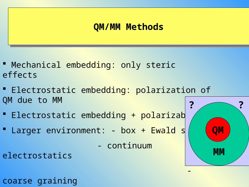
QM/MM MethodsQM/MM Methods

Mechanical embedding: only steric effects

Electrostatic embedding: polarization of QM due to MM

Electrostatic embedding + polarizable MM

Larger environment: - box + Ewald summ.

- continuum electrostatics

- coarse grainingMM

QM

? ?

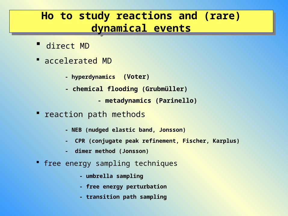
Ho to study reactions and (rare) dynamical eventsHo to study reactions and (rare) dynamical events

direct MD

accelerated MD

- hyperdynamics (Voter)

- chemical flooding (Grubmüller)

- metadynamics (Parinello)

reaction path methods

- NEB (nudged elastic band, Jonsson)

- CPR (conjugate peak refinement, Fischer, Karplus)

- dimer method (Jonsson)

free energy sampling techniques

- umbrella sampling

- free energy perturbation

- transition path sampling

Ho to study reactions and (rare) dynamical eventsHo to study reactions and (rare) dynamical events

accelerated MD

- metadynamics

reaction path methods- CPR

free energy sampling techniques

- umbrella sampling

QM/MM MethodsQM/MM Methods

Subtractive vs. additive modelsSubtractive vs. additive models

- subtractive: several layers: QM-MM

doublecounting on the regions is subtracted

- additive: different methods in different regions +

interaction between the regions

MM

QM

Additive QM/MMAdditive QM/MM

total energy QM= +

QM+

MM

MM

interaction

Subtractive QM/MM: ONIOM Morokuma and co.: GAUSSIAN

Subtractive QM/MM: ONIOM Morokuma and co.: GAUSSIAN

total energy

QM

MM=

-+ MM

The ONIOM Method (an ONION-like method)First LayerBond-formation/breaking takes place. Use the "High level" (H) method.

Second LayerElectronic effect on the first layer. Use the "Medium level" (M) method.

Third LayerEnvironmental effects on the first layer. Use the "Low level" (L) method.

Sm

all

Mo

del

S

yste

m (

SM

)

Inte

rmed

iate

M

od

el S

yste

m (

IM)

Rea

l S

yste

m (

R)

Example: The binding energy of 3C-C 3HPE)

C C

Hexaphenylethane

C

(HPE)

2

Triphenylmethyl radical

(TPMR)

ONIOM: 16.4 kcal/mol

from S. Irle

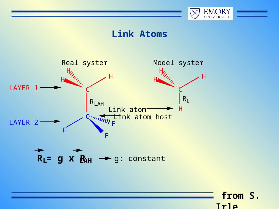
Link Atoms

C

C

FF

F

HHH

C

H

HHH

Link atomLink atom host

RL = g x RLAH

RLAH

LAYER 1

LAYER 2

Real system Model system

RL

g: constant

from S. Irle

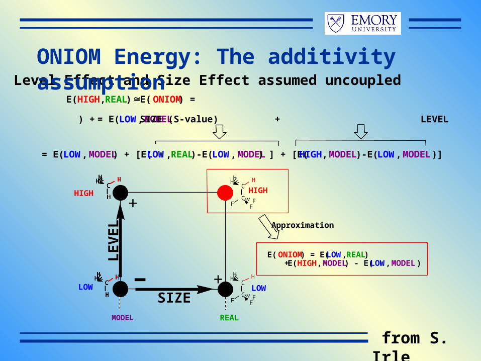
E(ONIOM) = E(LOW,REAL) + E(HIGH,MODEL) - E(LOW,MODEL)

C

CF F

F

HHH

C

CF F

F

HHH

C

H

HHH

C

H

HHH

C

H

HHH

C

H

HHH

C

H

HHH

C

H

HHH

C

H

HHH

C

H

HHH

C

H

HHH

C

H

HHH

C

H

HHH

C

H

H

HIGH HIGHHH

LOW LOW

SIZE

LE

VE

LE(HIGH,REAL) E(ONIOM) =

= E(LOW,MODEL) + SIZE (S-value) + LEVEL

Level Effect and Size Effect assumed uncoupled

Approximation

+

+-MODEL REAL

= E(LOW,MODEL) + [E(LOW,REAL)-E(LOW,MODEL) ] + [E(HIGH,MODEL)-E(LOW,MODEL)]

ONIOM Energy: The additivity assumption

from S. Irle

Choice of combination of levels is critical

S(ubstituent)-Value test: Does the low level work?

MODEL REAL

S(LOW)

LE

VE

L

SIZE

S(HIGH)If S(HIGH) = S(LOW)

E(ONIOM) = E( HIGH,REAL)

LOW

HIGH

Low level describes substituent effect as good as high level does!

Must be as close to zero as possible

S(HIGH) - S(LOW)

Combinations can be investigated using the S-Value test

Several E(HIGH,REAL) calculations necessary

S(LEVEL) = E(LEVEL,REAL) - E(LEVEL,MODEL)

from S. Irle

ONIOM Potential Energy Surface and PropertiesONIOM energy E(ONIOM, Real) = E(Low,Real) + E(High,Model) - E(Low,Model)

Potential energy surface well defined, and also derivatives are available.

ONIOM gradient G(ONIOM, Real) = G(Low,Real) + G(High,Model) x J - E(Low,Model) x J

J = (Real coord.)/ (Model coord.) is the Jacobian that converts the model system coordinate to the real system coordinate

ONIOM Hessian H(ONIOM,Real) = H(Low,Real) + JT x H(High,Model) x J - JT x H(Low,Model) x J

Scale each Hessian by s(Low)**2 or s(High)**2 to get scaled H(ONIOM)

ONIOM density (ONIOM, Real) = (Low,Real) + (High,Model) - (Low,Model)

ONIOM properties < o (ONIOM, Real)> = < o (Low,Real) > + < o (High,Model) > - < o (Low,Model) >

from S. Irle

Three-layer ONIOM (ONIOM3)

SIZE

LE

VE

L

MODEL REALINTERMEDIATE

LOW

MEDIUM

HIGH

E(ONIOM)= E(LOW,REAL)

- E(MEDIUM,MODEL)

+ E(HIGH,MODEL)

+ E(MEDIUM,INTERMEDIATE)

- E(LOW,INTERMEDIATE) +

+

+-

-MO:MO:MOMO:MO:MM

Target

from S. Irle

Additive QM/MM: linkingAdditive QM/MM: linking

Additive QM/MMAdditive QM/MM

total energy QM= +

QM+

MM

MM

interaction

/ˆ ˆ ˆ ˆ

QM MM QM MMH H H H

M

coorMMQM

M

M

M

M

Mi M M

M

iM

MMMQM H

R

B

R

A

R

qZ

r

qH

,

.int/612

, ,/

ˆˆ

Additive QM/MM: Additive QM/MM:

Elecrostatic mechanical embedding

Combined QM/MMCombined QM/MM

Amaro , Field , Chem Acc. 2003Bonds:

a) take force field terms

b) - link atom

- pseudo atoms

- frontier bonds

Nonbonding:

- VdW

- electrostatics

M

coorMMQM

M

M

M

M

Mi M M

M

iM

MMMQM H

R

B

R

A

R

qZ

r

qH

,

.int/612

, ,/

ˆˆ

Combined QM/MMCombined QM/MM

Reuter et al, JPCA 2000

Bonds:

a)

from force field

Combined QM/MM: link atomCombined QM/MM: link atom

Amaro & Field , T. Chem Acc. 2003

a) constrain or not?

(artificial forces)

relevant for MD

b) Electrostatics

- LA included – excluded

(include!)

- QM-MM:

exclude MM-host

exclude MM-hostgroup

- DFT, HF: gaussian broadening of MM point charges, pseudopotentails (e spill out)

Combined QM/MM: frozen orbitalsCombined QM/MM: frozen orbitals

Warshel, Levitt 1976

Rivail + co. 1996-2002

Gao et al 1998

M

coorMMQM

M

M

M

M

Mi M M

M

iM

MMMQM H

R

B

R

A

R

qZ

r

qH

,

.int/612

, ,/

ˆˆ

Reuter et al, JPCA 2000

Combined QM/MM: PseudoatomsCombined QM/MM: Pseudoatoms

Amaro & Field ,T Chem Acc. 2003

Pseudobond- connection atom

Zhang, Lee, Yang, JCP 110, 46

Antes&Thiel, JPCA 103 9290

No link atom: parametrize C H2 as pseudoatom

X

M

coorMMQM

M

M

M

M

Mi M M

M

iM

MMMQM H

R

B

R

A

R

qZ

r

qH

,

.int/612

, ,/

ˆˆ

Nonbonding terms:

VdW

- take from force field

- reoptimize for QM level

Coulomb:

which charges?

M

coorMMQM

M

M

M

M

Mi M M

M

iM

MMMQM H

R

B

R

A

R

qZ

r

qH

,

.int/612

, ,/

ˆˆ

Combined QM/MMCombined QM/MM

Amaro & Field ,T Chem Acc. 2003

Tests:

- C-C bond lengths, vib. frequencies

- C-C torsional barrier

- H-bonding complexes

- proton affinities, deprotonation

energies

Combined QM/MMCombined QM/MM

Subtractive vs. additive QM/MMSubtractive vs. additive QM/MM

- parametrization of methods for all regions required

e.g. MM for Ligands

SE for metals

+ QM/QM/MM conceptionally simple and applicable

Local Orbital vs. plane wave approaches:Local Orbital vs. plane wave approaches:

PW implementations

(most implementations in LCAO)

- periodic boundary conditions and large box! lots of empty space in unit cell

- hybride functionals have better accuracy: B3LYP, PBE0 etc.

+ no BSSE

+ parallelization (e.g. DNA with ~1000 Atoms)

• QM and MM accuracy

• QM/MM coupling

• model setup: solvent, restraints

• PES vs. FES: importance of sampling

All these factors CAN introduce errors in similar magnitude

ProblemsProblems

Modelling StratgiesModelling Stratgies

How much can we treat ? =How much can we afford

How much can we treat ? =How much can we afford

ProteinMembrane: = 4 Membrane: = 4

active

Water: = 80

Water: = 80

= 20

= 20

How to model the environmentHow to model the environment

1) Only QM (implicit solvent)

2) QM/MM w/wo MM polarization

3) Truncated systems and charge scaling

System in water with periodic boundary conditions: pbc and Ewald summation

Truncated system and implicit solvent models

How much can we treat ? =How much can we afford

How much can we treat ? =How much can we afford

Don‘t have or don‘t trust QM/MM or too complicated Only active site models

= ??

active

How much can we treat ? =How much can we afford

How much can we treat ? =How much can we afford

Protein

active

Small protein

Simple QM/MM: - fix most of the protein

- neglect polarization of environment

• solvation charge scaling

• freezing vs. stochastic boundary

• size of movable MM?

• size of QM?

First approximations: First approximations:

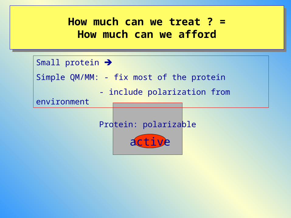
How much can we treat ? =How much can we afford

How much can we treat ? =How much can we afford

Protein: polarizable

active

Small protein

Simple QM/MM: - fix most of the protein

- include polarization from environment

Absolute excitation energies

S1 excitation energy (eV)

exp TD-B3LYP1

TD-DFTB

OM2/

CIS

CASSCF2 OM2/

MRCI

SORCI

vacuum 2.42 2.14 2.34 2.86 2.13 1.86

bR (QM:RET) 2.18

2.53 2.21 2.54 3.94 2.53 2.341Vreven[2003] 2 Hayashi[2000]

• TDDFT nearly zero

• CIS shifts still too small ~50%

• SORCI, CASPT2

• OM2/MRCI compares very well

0.1 0.2 1.0 0.5

Polarizable force field for environment

• MM charges

• MM polarization

RESP charges for residues in gas phase

atomic polarizabilities: = E

Polarization red shift of about 0.1 eV:

How much can we treat ? =How much can we afford

How much can we treat ? =How much can we afford

Explicit Watermolecules

pbc

Protein

active

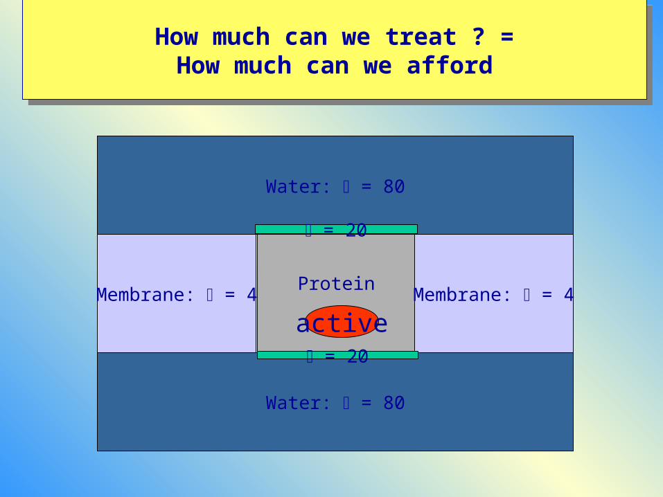
How much can we treat ? =How much can we afford

How much can we treat ? =How much can we afford

ProteinMembrane: = 4 Membrane: = 4

active

Water: = 80

Water: = 80

= 20

= 20

Ion channelsIon channels

Membrane: = 4 Membrane: = 4

Water: = 80

Water: = 80

Explicit water

Explicit water

Implicit solvent: Generalized Solvent Boundary Potential (GSBP, B. Roux)

Implicit solvent: Generalized Solvent Boundary Potential (GSBP, B. Roux)

•Drawback of conventional implicit solvation: e.g. specific water molecules important

•Compromise: 2 layers, one explicit solvent layer before implicit solvation model.

• inner region: MD, geomopt

• outer region: fixed QM/MM

explicit MM

implicit

GSBPGSBP

Solvation free energy of point charges

rf s v

GSBPGSBP

Depends on inner coordinates!

Basis set expansion of inner density calculate reaction field for basis set

QM/MM DFTB implementation by Cui group (Madison)

Water structure in AquaporinWater structure in Aquaporin

Water structure only in agreement with full solvent simulations when GSBP is used!

-differences in protein

conformations

Problems with the PES: CPR, NEB etc.Problems with the PES: CPR, NEB etc.

Zhang et al JPCB 107 (2003) 44459

- differences in protein conformations

(starting the reaction path calculation)

- problems along the reaction pathway

* flipping of water molecules

* size of movable MM region

different H-bonding pattern

average over these effects:

potential of mean force/free energy

Problems with the PES: complex energy landscape

Problems with the PES: complex energy landscape

Ion channelsIon channels