Quantum perceptron over a field and neural network architecture selectionin a quantum computer

Adenilton Jose da Silvaa,b, Teresa Bernarda Ludermirb, Wilson Rosa de Oliveiraa

aDepartamento de Estatıstica e InformaticaUniversidade Federal Rural de Pernambuco

bCentro de Informatica, Universidade Federal de PernambucoRecife, Pernambuco, Brasil

Abstract

In this work, we propose a quantum neural network named quantum perceptron over a field (QPF). Quantumcomputers are not yet a reality and the models and algorithms proposed in this work cannot be simulatedin actual (or classical) computers. QPF is a direct generalization of a classical perceptron and solves somedrawbacks found in previous models of quantum perceptrons. We also present a learning algorithm namedSuperposition based Architecture Learning algorithm (SAL) that optimizes the neural network weights andarchitectures. SAL searches for the best architecture in a finite set of neural network architectures withlinear time over the number of patterns in the training set. SAL is the first learning algorithm to determineneural network architectures in polynomial time. This speedup is obtained by the use of quantum parallelismand a non-linear quantum operator.

Keywords: Quantum neural networks, Quantum computing, Neural networks

1. Introduction

The size of computer components reduces each year and quantum effects have to be eventually consideredin computation with future hardware. The theoretical possibility of quantum computing initiated withBenioff [1] and Feynman [2] and the formalization of the first quantum computing model was proposed byDeutsch in 1985 [3]. The main advantage of quantum computing over classical computing is the use of aprinciple called superposition which allied with the linearity of the operators allows for a powerful form ofparallelism to develop algorithms more efficient than the known classical ones. For instance, the Grover’ssearch algorithm [4] and Shor’s factoring algorithm [5] overcome any known classical algorithm.

Quantum computing has recently been used in the development of new machine learning techniques asquantum decision trees [6], artificial neural networks [7, 8, 9], associative memory [10, 11], and inspired thedevelopment of novel evolutionary algorithms for continuous optimization problems [12, 13]. There is anincreasing interest in quantum machine learning and in the quantum neural network area [14]. This paperproposes a quantum neural network named Quantum Perceptron over a Field (QPF) and investigates the useof quantum computing techniques to design a learning algorithm for neural networks. Empirical evaluationof QPF and its learning algorithm needs of a quantum computer with thousands of qubits. Such quantumcomputer is not available nowadays and an empirical analysis of the QPF and its learning algorithm is notpossible with current technology.

Artificial neural networks are a universal model of computation [15] and have several applications inreal life problems. For instance, in the solution of combinatorial optimization problems [16], pattern recog-nition [17], but have some problems as the lack of an algorithm to determine optimal architectures [18],memory capacity and high cost learning algorithms [19].

∗A. J. da SilvaEmail address: adenilton.silva@ufrpe.br (Adenilton Jose da Silva)

Preprint submitted to Neural Networks November 28, 2015

arX

iv:1

602.

0070

9v1

[qu

ant-

ph]

29

Jan

2016

Notions of Quantum Neural Networks have been put forward since the nineties [20], but a precisedefinition of what is a quantum neural network that integrates neural computation and quantum computationis a non-trivial open problem [14]. To date, the proposed models in the literature are really just quantuminspired in the sense that despite using a quantum representation of data and quantum operators, in away or another some quantum principles are violated usually during training. Weights adjustments needmeasurements (observation) and updates.

Research in quantum neural computing is unrelated, as stated in [14]:

“QNN research remains an exotic conglomeration of different ideas under the umbrella of quan-tum information”.

and there is no consensus of what are the components of a quantum neural network. Several modelsof quantum neural networks have been proposed and they present different conceptual models. In somemodels a quantum neural network is described as a physical device [7]; as a model only inspired in quantumcomputing [21]; or as a mathematical model that explores quantum computing principles [22, 8, 9, 23]. Wefollow the last approach and assume that our quantum neural network model would be implemented in aquantum computer that follows the quantum principles as e.g. described in [24]. We assume that our modelsare implemented in the quantum circuit model of Quantum Computing [24].

Some advantages of quantum neural models over the classical models are the exponential gain in memorycapacity [25], quantum neurons can solve nonlinearly separable problems [22], and a nonlinear quantumlearning algorithm with polynomial time over the number of patterns in the data set is presented in [8].However, these quantum neural models cannot be viewed as a direct generalization of a classical neuralnetwork and have some limitations presented in Section 4. Quantum computing simulation has exponentialcost in relation to the number of qubits. Experiments with benchmarks and real problems are not possiblebecause of the number of qubits necessary to simulate a quantum neural network.

The use of artificial neural networks to solve a problem requires considerable time for choosing parametersand neural network architecture [26]. The architecture design is extremely important in neural networkapplications because a neural network with a simple architecture may not be capable of performing thetask. On the other hand, a complex architecture can overfit the training data [18]. The definition ofan algorithm to determine (in a finite set of architectures) the best neural network architecture (minimalarchitecture for a given learning task that can learn the training dataset) efficiently is an open problem. Theobjective of this paper is to show that with the supposition of non-linear quantum computing [8, 27, 28] wecan determine an architecture that can learn the training data in linear time with relation to the number ofpatterns in the training set. To achieve this objective, we propose a quantum neural network that respectthe principles of quantum computation, neural computing and generalizes the classical perceptron. Theproposed neuron works as a classical perceptron when the weights are in the computational basis, but asquantum perceptron when the weights are in superposition. We propose a neural network learning algorithmwhich uses a non-linear quantum operator [8, 28] to perform a global search in the space of weights andarchitecture of a neural network. The proposed learning algorithm is the first quantum algorithm performingthis kind of optimization in polynomial time and presents a framework to develop linear quantum learningalgorithms to find near optimal neural network architectures.

The remainder of this paper is divided into 6 Sections. In Section 2 we describe models that are outof the scope of this work. In Section 3 we present preliminary concepts of quantum computing necessaryto understand this work. In Section 4 we present related works. Section 5 presents main results of thispaper. We define the new model of a quantum neuron named quantum perceptron over a field that respectprinciples of quantum and neural computing. Also in Section 5 we propose a quantum learning algorithmfor neural networks that determines a neural network architecture that can learn the train set with somedesired accuracy. Section 6 presents a discussion. Finally, Section 7 is the conclusion.

2. Out of scope

Quantum computing and neural networks are multidisciplinary research fields. In this way, the quantumneural computing research is also multidisciplinary and concepts from physics, mathematics and computer

2

science are used. Probably because of this multidisciplinary characteristic there are completely differentconcepts named quantum neural networks. In this Section, we point some models that are out of the scopeof this work.

2.1. Quantum inspired neural networks

Neural networks whose definition is based on quantum computation, but that works in a classical com-puter as in [21, 29, 30] are named in this work as Quantum Inspired Neural Networks. Quantum inspiredneural networks are not real quantum models. Quantum inspired models are classical neural networks thatare inspired in quantum computing exactly as there are combinatorial optimization methods inspired in antcolony or bird swarm.

In [21] a complex neural network named qubit neural network whose neurons acts in the phase of theinput values is proposed. The qubit neural network has its functionality based in quantum operation, butit is a classical model and can be efficiently simulated in a classical computer.

Another quantum inspired models is defined in [31] where the activation function is a linear combinationof sigmoid functions. This linear combination of activation functions is inspired in the concept of quantumsuperposition, but these models can be efficiently simulated by a classical computer.

Quantum inspiration can bring useful new ideas and techniques for neural network models and learningalgorithms design. However, quantum inspired neural networks are out of the scope of this work.

2.2. Physical device quantum neural networks

Devices that implement a quantum neural network are proposed in [7, 32]. In this work, these models arenamed physical device quantum neural network. The main problem of this kind of proposal is the hardwaredependence. Scalable quantum computers are not yet a reality and when someone build a quantum computerwe do not know which hardware will be used.

In [7] a quantum neural network is represented by the architecture of a double slit experiment whereinput patterns are represented by photons, neurons are represented by slits, weights are represented bywaves and screen represents output neurons. In [32] a quantum neural network is represented by a quantumdot molecule evolving in real time. Neurons are represented by states of molecules, weights are the numberof excitations that are optically controlled, inputs are the initial state of the quantum dot molecules andoutputs are the final state of the dot molecules.

Physical device quantum neural networks are real quantum models. This kind of quantum neural net-works needs of specific hardware and is out of the scope of this work.

2.3. Quantum inspired algorithms

In this work algorithms whose development uses ideas from quantum computing, but run in a classicalcomputer are named quantum inspired algorithms. For instance, there are several quantum inspired evo-lutionary algorithm proposed in literature [33, 34, 35, 36, 37, 38]. This kind of algorithm uses quantuminspiration to define better classical algorithms, but intrinsic quantum properties are not used. Quantuminspired algorithms are out of the scope of this work.

3. Quantum computing

In this Section, we perform a simple presentation of quantum computing with the necessary conceptsto understand the following sections. As in theoretical classical computing we are not interested in howto store or physically represent a quantum bit. Our approach is a mathematical. We deal with how wecan abstractly compute with quantum bits or design abstract quantum circuits and models. We take as aguiding principle that when a universal quantum computer will be at our disposal, we could implement theproposed quantum neural models.

3

We define a quantum bit as unit complex bi-dimensional vector in the vector space C2. In the quantumcomputing literature a vector is represented by the Diracs notation |·〉. The computational basis is the set{|0〉, |1〉}, where the vectors |0〉 and |1〉 can be represented as in Equation (1).

|0〉 =

[10

]and |1〉 =

[01

](1)

A quantum bit |ψ〉, qubit, is a vector in C2 that has a unit length as described in Equation (2), where|α|2 + |β|2 = 1, α, β ∈ C.

|ψ〉 = α|0〉+ β|1〉 (2)

While in classical computing there are only two possible bits, 0 or 1, in quantum computing there arean infinitely many quantum bits, a quantum bit can be a linear combination (or superposition) of |0〉 and|1〉. The inner product of two qubits |ψ〉 and |θ〉 is denoted as 〈ψ|θ〉 and the symbol 〈ψ| is the transposeconjugate of the vector |ψ〉.

Tensor product ⊗ is used to define multi-qubit systems. On the vectors, if |ψ〉 = α0|0〉 + α1|1〉 and|φ〉 = β0|0〉 + β1|1〉, then the tensor product |ψ〉 ⊗ |φ〉 is equal to the vector |ψφ〉 = |ψ〉 ⊗ |φ〉 = (α0|0〉 +α1|1〉) ⊗ (β0|0〉 + β1|1〉) = α0β0|00〉 + α0β1|01〉 + α1β0|10〉 + α1β1|11〉. Quantum states representing nqubits are in a 2n dimensional complex vector space. On the spaces, let X ⊂ V and X′ ⊂ V′ be basis ofrespectively vector spaces V and V′. The tensor product V⊗V′ is the vector space obtained from the basis{|b〉 ⊗ |b′〉; |b〉 ∈ X and |b′〉 ∈ X′}. The symbol V⊗n represents a tensor product V⊗ · · · ⊗ V with n factors.

Quantum operators over n qubits are represented by 2n × 2n unitary matrices. An n × n matrix U isunitary if UU† = U†U = I, where U† is the transpose conjugate of U. For instance, identity I, the flip X,and the Hadamard H operators are important quantum operators over one qubit and they are described inEquation (3).

I =

[1 00 1

]X =

[0 11 0

]H = 1√

2

[1 11 −1

](3)

The operator described in Equation (4) is the controlled not operator CNot, that flips the second qubit ifthe first (the controlled qubit) is the state |1〉.

CNot =

1 0 0 00 1 0 00 0 0 10 0 1 0

(4)

Parallelism is one of the most important properties of quantum computation used in this paper. Iff : Bm → Bn is a Boolean function, B = {0, 1}, one can define a quantum operator

Uf :(C2)⊗n+m → (

C2)⊗n+m

, (5)

asUf |x, y〉 = |x, y ⊕ f(x)〉,

where ⊕ is the bitwise xor, such that the value of f(x) can be recovered as

Uf |x, 0〉 = |x, f(x)〉.

The operator Uf is sometimes called the quantum oracle for f . Parallelism occurs when one applies theoperator Uf to a state in superposition as e.g. described in Equation (6).

Uf

(n∑i=0

|xi, 0〉

)=

n∑i=0

|xi, f(xi)〉 (6)

The meaning of Equation (6) is that if one applies operator Uf to a state in superposition, by linearity, thevalue of f(xi), will be calculated for each i simultaneously with only one single application of the quantumoperator Uf .

4

With quantum parallelism one can imagine that if a problem can be described with a Boolean function fthen it can be solved instantaneously. The problem is that one cannot direct access the values in a quantumsuperposition. In quantum computation a measurement returns a more limited value. The measurement ofa quantum state |ψ〉 =

∑ni=1 αi|xi〉 in superposition will return xi with probability |αi|2. With this result

the state |ψ〉 collapses to state |xi〉, i.e., after the measurement |ψ〉 = |xi〉.

4. Related works

Quantum neural computation research started in the nineties [20], and the models (such as e.g. in [7,8, 22, 39, 9, 40, 41, 42]) are yet unrelated. We identify two types of quantum neural networks: 1) modelsdescribed mathematically to work on a quantum computer (as in [39, 40, 22, 8, 43, 9, 44, 45]); 2) modelsdescribed by a quantum physical device (as in [7, 32]). In the following subsections we describe some modelsof quantum neural networks.

4.1. qANN

Altaisky [39] proposed a quantum perceptron (qANN). The qANN N is described as in Equation (7),

|y〉 = F

n∑j=1

wj |xj〉 (7)

where F is a quantum operator over 1 qubit representing the activation function, wj is a quantum operatorover a single qubit representing the j-th weight of the neuron and |xj〉 is one qubit representing the inputassociated with wj .

The qANN is one of the first models of quantum neural networks. It suggests a way to implement theactivation function that is applied (and detailed) for instance in [8].

It was not described in [39] how one can implement Equation (7). An algorithm to put patterns insuperposition is necessary. For instance, the storage algorithm of a quantum associative memory [25] canbe used to create the output of the qANN. But this kind of algorithm works only with orthonormal states,as shown in Proposition 4.1.

Proposition 4.1. Let |ψ〉 and |θ〉 be two qubits with probability amplitudes in R, if 1√2

(|ψ〉+ |θ〉) is a unit

vector then |ψ〉 and |θ〉 are orthogonal vectors.

Proof Let |ψ〉 and |θ〉 be qubits and suppose that 1√2

(|ψ〉+ |θ〉) is a unit vector. Under these conditions

1

2(|ψ〉+ |θ〉, |ψ〉+ |θ〉) = 1⇒

1

2(〈ψ|ψ〉+ 〈ψ|θ〉+ 〈θ|ψ〉+ 〈θ|θ〉) = 1

Qubits are unit vectors, then1

2(2 + 2 〈ψ|θ〉) = 1 (8)

and |ψ〉 and |θ〉 must be orthogonal vectors.

A learning rule for the qANN has been proposed and it is shown that the learning rule drives theperceptron to the desired state |d〉 [39] in the particular case described in Equation (9) where is supposedthat F = I. But this learning rule does not preserve unitary operators [9].

wj(t+ 1) = wj(t) + η (|d〉 − |y(t)〉) 〈xj | (9)

In [44] a quantum perceptron named Autonomous Quantum Perceptron Neural Network (AQPNN) isproposed. This model has a learning algorithm that can learn a problem in a small number of iterationswhen compared with qANN and these weights are represented in a quantum operator as the qANN weights.

5

4.2. qMPN

Proposition 4.1 shows that with the supposition of unitary evolution, qANN with more than one inputis not a well defined quantum operator. Zhou and Ding proposed a new kind of quantum perceptron [22]which they called as quantum M-P neural network (qMPN). The weights of qMPN are stored in a singlesquared matrix W that represents a quantum operator. We can see the qMPN as a generalized single weightqANN, where the weight is a quantum operator over any number of qubits. The qMPN is described inEquation (10), where |x〉 is an input with n qubits, W is a quantum operator over n qubits and |y〉 is theoutput.

|y〉 = W |x〉 (10)

They also proposed a quantum learning algorithm for the new model. The learning algorithm for qMPNis described in Algorithm 1. The weights update rule of Algorithm 1 is described in Equation (11),

wt+1ij = wtij + η (|d〉i − |y〉i) |x〉j (11)

where wij are the entries of the matrix W and η is a learning rate.

Algorithm 1 Learning algorithm qMPN

1: Let W (0) be a weight matrix2: Given a set of quantum examples in the form (|x〉, |d〉), where |x〉 is an input and |d〉 is the desired

output3: Calculate |y〉 = W (t)|x〉, where t is the iteration number4: Update the weights following the learning rule described in Equation (11).5: Repeat steps 3 and 4 until a stop criterion is met.

The qMPN model has several limitations in respect to the principles of quantum computing. qMPN isequivalent to a single layer neural network and its learning algorithm leads to non unitary neurons as shownin [46].

4.3. Neural network with quantum architecture

In the last subsections the neural network weights are represented by quantum operators and the inputsare represented by qubits. In the classical case, inputs and free parameters are real numbers. So one canconsider to use qubits to represent inputs and weights. This idea was used, for instance, in [40, 8]. In [40]a detailed description of the quantum neural network is not presented.

In [8] a Neural Network with Quantum Architecture (NNQA) based on a complex valued neural networknamed qubit neural network [21] is proposed. Qubit neural network is not a quantum neural network beingjust inspired in quantum computing. Unlike previous models [39, 22], NNQA uses fixed quantum operatorsand the neural network configuration is represented by a string of qubits. This approach is very similar tothe classical case, where the neural network configuration for a given architecture is a string of bits.

Non-linear activation functions are included in NNQA in the following way. Firstly is performed adiscretization of the input and output space, the scalars are represented by Boolean values. In doing so aneuron is just a Boolean function f and the quantum oracle operator for f , Uf , is used to implement thefunction f acting on the computational basis.

In the NNQA all the data are quantized with Nq bits. A synapses of the NNQA is a Boolean functionf0 : B2Nq → BNq . A synapses of the NNQA is a Boolean function described in Equation (12).

z = arctan

(sin(y) + sin(θ)

cos(y) + cos(θ)

)(12)

6

The values y and θ are angles in the range [−π/2, π/2] representing the argument of a complex num-ber, which are quantized as described in Equation (13). The representation of the angle β is the binaryrepresentation of the integer k.

β = π

(−0.5 +

k

2Nq − 1

), k = 0, 1, · · · , 2Nq − 1 (13)

Proposition 4.2. The set F = {βk|βk = π · (−0.5+ k/(2Nq − 1)), k = 0, · · · , 2Nq − 1

}with canonical ad-

dition and multiplication is not a field.

Proof We will only show that the additive neutral element is not in the set. Suppose that 0 ∈ F . So,

π ·(−0.5 +

k

2Nq − 1

)= 0⇒ −0.5 +

k

2Nq − 1= 0

⇒ k

2Nq − 1= 0.5⇒ k = (2Nq − 1) ·

(−1

2

)Nq is a positive integer, and 2Nq−1 is an odd positive integer, then (2Nq−1) ·

(− 1

2

)/∈ Z which contradicts

the assumption that k ∈ Z and so F is not a field since 0 /∈ F .

From Proposition 4.2 we conclude that the we cannot directly lift the operators and algorithms fromclassical neural networks to NNQA. In a weighted neural network inputs and parameters are rational, realor complex numbers and the set of possible weights of NNQA under operations defined in NNQA neuron isnot a field.

5. Quantum neuron

5.1. Towards a quantum perceptron over a field

In Definition 5.1 and Definition 5.1 we have, respectively, an artificial neuron and a classical neuralnetwork as in [47]. Weights and inputs in classical artificial neural networks normally are in the set of real(or complex) numbers.

Definition An artificial neuron is described by the Equation (14), where x1, x2, · · · , xk are input signalsand w1, w2, · · · , wk are weights of the synaptic links, f(·) is a nonlinear activation function, and y is theoutput signal of the neuron.

y = f

m∑j=0

wjxj

(14)

In both qANN and qMPN artificial neurons, weights and inputs are in different sets (respectively inquantum operators and qubits) while weights and inputs in a classical perceptron are elements of the samefield. The NNQA model defines an artificial neuron where weights and inputs are strings of qubits. Theneuron is based on a complex valued network and does not exactly follow Definition 5.1. The main problemin NNQA is that the inputs and weights do not form a field with sum and multiplication values as we show inProposition 4.2. There is no guarantee that the set of discretized parameters is closed under the operationsbetween qubits.

Other models of neural networks where inputs and parameters are qubits were presented in [48, 49, 9].These models are a generalization of weightless neural network models, whose definitions are not similar toDefinition 5.1.

Definition A neural network is a directed graph consisting of nodes with interconnecting synaptic andactivation links, and is characterized by four properties [47]:

7

1. Each neuron is represented by a set of linear synaptic links, an externally applied bias, and a possibilitynon-linear activation link. The bias is represented by a synaptic link connected to an input fixed at+1.

2. The synaptic links of a neuron weight their respective input signals.

3. The weighted sum of the input signals defines the induced local field of the neuron in question.

4. The activation link squashes the induced local field of the neuron to produce an output.

The architecture of NNQA can be viewed as a directed graph consisting of nodes with interconnectingsynaptic and activation links as stated in Definition 5.1. The NNQA does not follow all properties of a neuralnetwork (mainly because it is based in the qubit NN), but it is one of the first quantum neural networks withweights and a well defined architecture. The main characteristics of the NNQA are that inputs and weightsare represented by a string of qubits, and network follows a unitary evolution. Based on these characteristicswe will propose the quantum perceptron over a field.

5.2. Neuron operations

We propose a quantum perceptron with the following properties: it can be trained with a quantumor classical algorithm, we can put all neural networks for a given architecture in superposition, and if theweights are in the computational basis the quantum perceptron acts like the classical perceptron. One of thedifficulties to define a quantum perceptron is that the set of n-dimensional qubits, sum and (tensor) productoperators do not form a field (as shown in Proposition 5.1). Therefore, the first step in the definition of thequantum perceptron is to define a new appropriate sum and multiplication of qubits.

Proposition 5.1. The set of qubits under sum + of qubits and tensor product ⊗ is not a field.

Proof The null vector has norm 0 and is not a valid qubit. Under + operator the null vector is unique, sothere is not a null vector in the set of qubits. Then we cannot use + operator to define a field in the set ofqubits.

Tensor product between two qubits results in a compound system with two qubits. So the space of qubitsis not closed under the ⊗ operator and we cannot use ⊗ operator to define a field in the set of qubits.

We will define unitary operators to perform sum ⊕ and product � of qubits based in the field operations.Then we will use these new operators to define a quantum neuron. Let F (⊕,�) be a finite field. We canassociate the values a ∈ F to vectors (or qubits) |a〉 in a basis of a vector space V. If F has n elements thevector space will have dimension n.

Product operation � in F can be used to define a new product between vectors in V. Let |a〉 and |b〉 bequbits associated with scalars a and b, we define |a〉�|b〉 = |a� b〉 such that |a� b〉 is related with the scalara � b. This product send basis elements to basis elements, so we can define a linear operator P : V3 → V3

as in Equation (15).

P|a〉|b〉|c〉 = |a〉|b〉|c⊕ (a� b)〉 (15)

We show in Proposition 5.2 that the P operator is unitary, therefore P is a valid quantum operator.

Proposition 5.2. P is a unitary operator.

Proof Let B = {|a1〉, |a2〉, · · · , |an〉} be a computational basis of a vector space V, where we associate|ai〉 with the element ai of the finite field F (⊕,�). The set B3 = {|ai〉|aj〉|ak〉} with 1 ≤ i, j, k ≤ n is acomputational basis of vector space V3. We will show that P sends elements of basis B3 in distinct elementsof basis B3.

P sends vectors in base B3 to vectors in base B3. Let a, b, c in B. P|a〉|b〉|c〉 = |a〉|b〉|c⊕ (a� b)〉.Operators ⊕ and � are well defined, then |c⊕ (a� b)〉 ∈ B and |a〉|b〉|c⊕ (a� b)〉 ∈ B3.

8

P is injective. Let a, b, c, a1, b1, c1 ∈ F such that P|a〉|b〉|c〉 = P|a1〉|b1〉|c1〉 . By the definition of operatorP a = a1 and b = b1 . When we apply the operator we get |a〉|b〉|c⊕ (a� b)〉 = |a〉|b〉|c1 ⊕ (a� b)〉. Thenc1 ⊕ (a� b) = c⊕ (a� b) . By the field properties we get c1 = c.

An operator over a vector space is unitary if and only if the operator sends some orthonormal basisto some orthonormal basis [50]. As P is injective and sends vectors in base B3 to vectors in base B3, weconclude that P is an unitary operator.

With a similar construction, we can use the sum operation ⊕ in F to define a unitary sum operatorS : V3 → V3. Let |a〉 and |b〉 be qubits associated with scalars a and b, we define |a〉 ⊕ |b〉 = |a⊕ b〉 suchthat |a⊕ b〉 is related with the scalar a⊕ b. We define the unitary quantum operator S in Equation (16).

S|a〉|b〉|c〉 = |a〉|b〉|c⊕ (a⊕ b)〉 (16)

We denote product and sum of vectors over F by |a〉 � |b〉 = |a� b〉 and |a〉 ⊕ |b〉 = |a⊕ b〉 to represent,respectively, P|a〉|b〉|0〉 = |a〉|b〉|a� b〉 and S|a〉|b〉|0〉 = |a〉|b〉|a⊕ b〉.

5.3. Quantum perceptron over a field

Using S and P operators we can define a quantum perceptron analogously as the classical one. Inputs|xi〉, weights |wi〉 and output |y〉 will be unit vectors (or qubits) in V representing scalars in a field F .Equation (17) describes the proposed quantum perceptron.

|y〉 =

n⊕i=1

|xi〉 � |wi〉 (17)

If the field F is the set of rational numbers, then Definition 5.1 without activation function f correspond toDefinition 17 when inputs, and weights are in the computational basis.

The definition in Equation (17) hides several ancillary qubits. The complete configuration of a quantumperceptron is given by the state |ψ〉 described in Equation (18),

|ψ〉 = |x1, · · · , xn, w1, · · · , wn,p1, · · · , pn, s2, · · · , sn−1, y〉

(18)

where |x〉 = |x1, · · · , xn〉 is the input quantum register, |w〉 = |w1, · · · , wn〉 is the weight quantum register,|p〉 = |p1, · · · , pn〉 is an ancillary quantum register used to store the products |xi � wi〉, |s〉 = |s2, · · · , sn−1〉 isan ancillary quantum register used to store sums, and |y〉 is the output quantum register. From Equation (18)one can see that to put several or all possible neural networks in superposition one can simply put the weightquantum register in superposition. Then a single quantum neuron can be in a superposition of severalneurons simultaneously.

A quantum perceptron over a finite d-dimensional field and with n inputs needs (4n − 1) · d quantumbits to perform its computation. There are n quantum registers to store inputs xi, n quantum registers tostore weights wi, n quantum registers pi to store the products wi � xi, n− 2 quantum registers |si〉 to store

sums∑ik=1 pi and one quantum register to store the output |y〉 =

∑nk=1 pi.

We show now a neuron with 2 inputs to illustrate the workings of the quantum neuron. SupposeF = Z2 = {0, 1}. As the field has only two elements we need only two orthonormal quantum states torepresent the scalars. We choose the canonical ones 0↔ |0〉 and 1↔ |1〉.

Now we define sum ⊕ and multiplication � operators based on the sum and multiplication in Z2. The

9

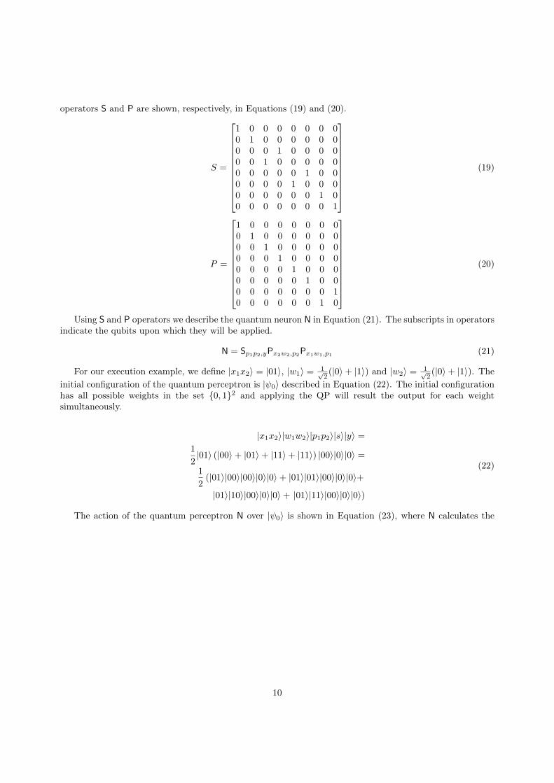
operators S and P are shown, respectively, in Equations (19) and (20).

S =

1 0 0 0 0 0 0 00 1 0 0 0 0 0 00 0 0 1 0 0 0 00 0 1 0 0 0 0 00 0 0 0 0 1 0 00 0 0 0 1 0 0 00 0 0 0 0 0 1 00 0 0 0 0 0 0 1

(19)

P =

1 0 0 0 0 0 0 00 1 0 0 0 0 0 00 0 1 0 0 0 0 00 0 0 1 0 0 0 00 0 0 0 1 0 0 00 0 0 0 0 1 0 00 0 0 0 0 0 0 10 0 0 0 0 0 1 0

(20)

Using S and P operators we describe the quantum neuron N in Equation (21). The subscripts in operatorsindicate the qubits upon which they will be applied.

N = Sp1p2,yPx2w2,p2Px1w1,p1 (21)

For our execution example, we define |x1x2〉 = |01〉, |w1〉 = 1√2(|0〉+ |1〉) and |w2〉 = 1√

2(|0〉+ |1〉). The

initial configuration of the quantum perceptron is |ψ0〉 described in Equation (22). The initial configurationhas all possible weights in the set {0, 1}2 and applying the QP will result the output for each weightsimultaneously.

|x1x2〉|w1w2〉|p1p2〉|s〉|y〉 =

1

2|01〉 (|00〉+ |01〉+ |11〉+ |11〉) |00〉|0〉|0〉 =

1

2(|01〉|00〉|00〉|0〉|0〉+ |01〉|01〉|00〉|0〉|0〉+

|01〉|10〉|00〉|0〉|0〉+ |01〉|11〉|00〉|0〉|0〉)

(22)

The action of the quantum perceptron N over |ψ0〉 is shown in Equation (23), where N calculates the

10

x1

x2

x3

∑

∑

∑

∑

∑

w11

w 12

w13

w21

w22

w 23

w31

w32

w33

w14

w24

w34

w15

w25

w 35

y1

y2

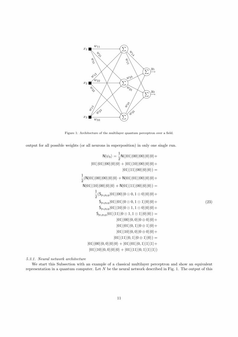
Figure 1: Architecture of the multilayer quantum perceptron over a field.

output for all possible weights (or all neurons in superposition) in only one single run.

N|ψ0〉 =1

2N(|01〉|00〉|00〉|0〉|0〉+

|01〉|01〉|00〉|0〉|0〉+ |01〉|10〉|00〉|0〉|0〉+|01〉|11〉|00〉|0〉|0〉) =

1

2(N|01〉|00〉|00〉|0〉|0〉+ N|01〉|01〉|00〉|0〉|0〉+

N|01〉|10〉|00〉|0〉|0〉+ N|01〉|11〉|00〉|0〉|0〉) =

1

2(Sp1p2y|01〉|00〉|0� 0, 1� 0〉|0〉|0〉+

Sp1p2y|01〉|01〉|0� 0, 1� 1〉|0〉|0〉+Sp1p2y|01〉|10〉|0� 1, 1� 0〉|0〉|0〉+

Sp1p2y|01〉|11〉|0� 1, 1� 1〉|0〉|0〉) =

|01〉|00〉|0, 0〉|0⊕ 0〉|0〉+|01〉|01〉|0, 1〉|0⊕ 1〉|0〉+|01〉|10〉|0, 0〉|0⊕ 0〉|0〉+|01〉|11〉|0, 1〉|0⊕ 1〉|0〉) =

|01〉|00〉|0, 0〉|0〉|0〉+ |01〉|01〉|0, 1〉|1〉|1〉+|01〉|10〉|0, 0〉|0〉|0〉+ |01〉|11〉|0, 1〉|1〉|1〉)

(23)

5.3.1. Neural network architecture

We start this Subsection with an example of a classical multilayer perceptron and show an equivalentrepresentation in a quantum computer. Let N be the neural network described in Fig. 1. The output of this

11

network can be calculated as y = L2 ·L1 ·x using the three matrices L1, L2 and x described in Equation (24).

L1 =

w11 w12 w13

w21 w22 w23

w31 w32 w33

,L2 =

[w14 w24 w34

w15 w25 w35

], x =

x1x2x3

(24)

Weights, inputs and outputs in a classical neural network are real numbers. Here we suppose finitememory and we use elements of a finite field (F,⊕,�) to represent the neural network parameters. Wecan define a quantum operator M3×3,3×1 that multiplies a 3 × 3 matrix with a 3 × 1 matrix. If L1 · x =[o1 o2 o3

]twe define the action of M3×3,3×1 in Equation (25), where wi = wi1, wi2, wi3.

M3×3,3×1|w1, w2, w3, x1, x2, x3, 0, 0, 0〉 =

|w1, w2, w3, x1, x2, x3, o1, o2, o3〉(25)

Each layer of the quantum perceptron over a field can be represented by an arbitrary matrix as inEquation (26),

M2×3,3×1M3×3,3×1|L2〉|L1〉|x〉|000〉|00〉 (26)

where M3×3,3×1 acts on |L1〉, |x〉 with output in register initialized with |000〉; and M2×3,3×1 acts on |L2〉,the output of the first operation, and the last quantum register. This matrix approach can be used torepresent any feed-forward multilayer quantum perceptron over a field with any number of layers.

We suppose here that the training set and desired output are composed of classical data and that thedata run forward. The supposition of classical desired output will allow us to superpose neural networkconfigurations with its performance, as we will see in the next section.

5.3.2. Learning algorithm

In this Subsection, we present a learning algorithm that effectively uses quantum superposition to traina quantum perceptron over a field. Algorithms based on superposition have been proposed previouslyin [8, 27, 51]. In these papers, a non-linear quantum operator proposed in [28], is used in the learningprocess. In [8] performances of neural networks in superposition are entangled with its representation. Anon-linear algorithm is used to recover a neural network configuration with performance greater than a giventhreshold θ. A non-linear algorithm is used to recover the best neural network configuration. In [27] thenonlinear quantum operator is used in the learning process of a neurofuzzy network. In [51] a quantumassociative neural network is proposed where a non-linear quantum circuit is used to increase the patternrecalling speed.

We propose a variant of the learning algorithm proposed in [8]. The proposed quantum algorithm isnamed Superposition based Architecture Learning (SAL) algorithm. In the SAL algorithm the superpositionof neural networks will store its performance entangled with its representation, as in [8]. Later we will usea non-linear quantum operator to recover the architecture and weights of the neural network configurationwith best performance.

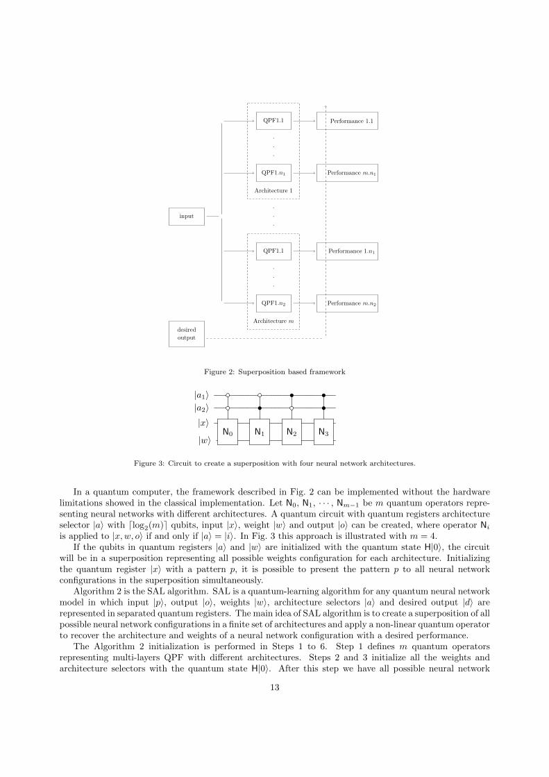
In the classical computing paradigm, the idea of presenting an input pattern to all possible neuralnetworks architectures is impracticable. To perform this idea classically one will need to create severalcopies of the neural network (one for each configuration and architecture) to receive all the inputs andcompute in parallel the corresponding outputs. After calculating the output of each pattern for each neuralnetwork configuration, one can search the neural configuration with best performance. Yet classically theidea of SAL learning is presented in Fig. 2. For some neural network architectures, all the patterns in thetraining set P = {p1, p2, · · · , pk} are presented to each of the neural network configurations. Outputs arecalculated and then one can search the best neural network parameters.

12

QPF1.1

.

.

.

QPF1.n1

Architecture 1

.

.

.

QPF1.1

.

.

.

QPF1.n2

Architecture m

input

desired

output

Performance 1.1

Performance m.n1

Performance 1.n1

Performance m.n2

Figure 2: Superposition based framework

|a1〉 • •|a2〉 • •|x〉

N0 N1 N2 N3|w〉

Figure 3: Circuit to create a superposition with four neural network architectures.

In a quantum computer, the framework described in Fig. 2 can be implemented without the hardwarelimitations showed in the classical implementation. Let N0, N1, · · · , Nm−1 be m quantum operators repre-senting neural networks with different architectures. A quantum circuit with quantum registers architectureselector |a〉 with dlog2(m)e qubits, input |x〉, weight |w〉 and output |o〉 can be created, where operator Niis applied to |x,w, o〉 if and only if |a〉 = |i〉. In Fig. 3 this approach is illustrated with m = 4.

If the qubits in quantum registers |a〉 and |w〉 are initialized with the quantum state H|0〉, the circuitwill be in a superposition representing all possible weights configuration for each architecture. Initializingthe quantum register |x〉 with a pattern p, it is possible to present the pattern p to all neural networkconfigurations in the superposition simultaneously.

Algorithm 2 is the SAL algorithm. SAL is a quantum-learning algorithm for any quantum neural networkmodel in which input |p〉, output |o〉, weights |w〉, architecture selectors |a〉 and desired output |d〉 arerepresented in separated quantum registers. The main idea of SAL algorithm is to create a superposition of allpossible neural network configurations in a finite set of architectures and apply a non-linear quantum operatorto recover the architecture and weights of a neural network configuration with a desired performance.

The Algorithm 2 initialization is performed in Steps 1 to 6. Step 1 defines m quantum operatorsrepresenting multi-layers QPF with different architectures. Steps 2 and 3 initialize all the weights andarchitecture selectors with the quantum state H|0〉. After this step we have all possible neural network

13

configurations for the given architectures in superposition. In Steps 5 and 6 quantum registers performanceand objective are initialized respectively, with the quantum states |0〉n and |0〉.

The for loop starting in Step 7 is repeated for each pattern p of the data set. Step 8 initializes quantumregisters p, o and d respectively with a pattern |p〉, state |0〉 and its desired output |d〉. Step 9 presents thepattern to the neural networks, and the outputs are calculated. In this moment, the pattern is present toall neural networks configurations, because the weights and architecture selectors quantum registers are in asuperposition of all possible weights and architectures. In Steps 10 to 12, it is verified for each configurationin the superposition if the desired output |d〉 is equal to the calculated output |o〉. If they match, is addedthe value 1 for the performance quantum register. Step 13 is performed to allow the initialization of thenext for loop.

|a〉|w〉|performance〉|objective〉 =∑w∈W,a∈A

|a〉|w〉|performance(w)〉|0〉 (27)

After the execution of the for loop, the state of quantum registers weights w, architecture selectors a,performance and objective can be described as in Equation (27), where A is the set of architectures and Wis the set of all possible weights.

Algorithm 2 SAL

1: Let N0, N1, · · · , Nm be quantum operators representing multi-layers QPF with different architectures.2: Create a quantum circuit where the i-th network acts if and only if |a〉 = |i〉.3: Initialize all weights quantum registers with the quantum state H|0〉.4: Initialize all architecture quantum registers with quantum state H|0〉.5: Initialize a quantum register |performance〉 with the state |0〉n.6: Initialize a quantum register |objective〉 with the state |0〉.7: for each pattern p and desired output d in the training set do8: Initialize the register p, o , d with the quantum state |p, 0, d〉.9: Calculate N|p〉 to calculate network output in register |o〉.

10: if |o〉 = |d〉 then11: Add 1 to the register |performance〉12: end if13: Calculate N−1|p〉 to restore |o〉.14: end for15: Perform a non-linear quantum search to recover a neural network configuration and architecture with

desired performance.

Steps 1 to 14 of Algorithm 2 can be performed using only linear quantum operators. In Step 15 a non-linear quantum operator NQ proposed in [28] will be used. Action of NQ is described in Equation (28) if atleast one |ci〉 is equal to |1〉 otherwise its action is described in Equation (29).

NQ

(∑i

|ψi〉|ci〉

)=

(∑i

|ψi〉

)|1〉 (28)

NQ

(∑i

|ψi〉|ci〉

)=

(∑i

|ψi〉

)|0〉 (29)

The non-linear search used in Step 15 is described in Algorithm 3. The for loop in Step 1 of Algorithm 3indicates that the actions need to be repeated for each quantum bit in the architecture and weights quantumregisters. Steps 3 to 5 set the objective quantum register |o〉 to |1〉 if the performance quantum register p

14

is greater than a given threshold θ. After this operation the state of quantum registers a, w and o can bedescribed as in Equation (30). ∑

w∈(P (a,w)<θ),|b〉6=|i〉

|a〉|w〉|0〉+∑

w∈(P (a,w)≥θ),|b〉=|i〉

|a〉|w〉|1〉 (30)

Now that quantum register objective is set to 1 in the desired configurations, it is possible to perform aquantum search to increase the probability amplitude of the best configurations.

Algorithm 3 Non-linear quantum search

1: for each quantum bit |b〉 in quantum registers |a〉|w〉 do2: for i = 0 to 1 do3: if |b〉 = |i〉 and |p〉 > θ then4: Set |o〉 to |1〉5: end if6: Apply NQ to |o〉7: if |o〉 = |1〉 then8: Apply Xi · NQ to qubit |b〉9: Apply X to |o〉

10: end if11: end for12: end for

Step 6 applies NQ to quantum register |o〉. If there is at least one configuration with |b〉 = |i〉 then theaction of NQ will set |o〉 to |1〉. In this case, Steps 7 to 10 set qubit |b〉 from a superposed state to thecomputational basis state |i〉.

Algorithm 3 performs an exhaustive non-linear quantum search in the architecture and weights space.If there is a neural network configuration with the desired performance in initial superposition, the searchwill return one of these configurations. Otherwise the algorithm does not change the initial superpositionand the procedure can be repeated with another performance threshold.

The computational cost of Steps 1 and 2 of SAL is O(m) and depends on the number of neural networksarchitectures. Steps 3 to 6 has computational cost O(m+nw), where nw is the number of qubits to representthe weights. The for starting in Step 7 will be executed p times and each inner line has constant cost. Step15 is detailed in Algorithm 3. Steps 3 to 9 of Algorithm 3 have constant computational cost and it will berepeated 2 · (m+ nw) times. The overall cost of the SAL algorithm is O(p+m+nw) where p is the numberof patterns in the training set.

6. Discussion

Classical neural networks have limitations, such as i) the lack of an algorithm to determine optimalarchitectures, ii) memory capacity and iii) high cost learning algorithms. In this paper, we investigate howto use quantum computing to deal with limitation iii). To achieve this objective, we define a quantum neuralnetwork model named quantum perceptron over a field QPF and a nonlinear quantum learning algorithmthat performs an exhaustive search in the space of weights and architectures.

We have shown that previous models of quantum perceptron cannot be viewed as a direct quantizationof the classical perceptron. In other models of quantum neural networks weights and inputs are representedby a string of qubits, but the set of all possible inputs and weights with inner neuron operations does notform a field and there is no guarantee that they are well defined operations. To define QPF we proposequantum operators to perform addition and multiplication such that the qubits in a computational basisform a field with these operations. QPF is the unique neuron with these properties. We claim that QPF canbe viewed as a direct quantization of a classical perceptron, since when the qubits are in the computational

15

Figure 4: Relation between the number of qubits n and size of quantum operators with matricial representation in R2n×2n

using standard C++ floating point precision

basis the QPF acts exactly as a classical perceptron. In this way, theoretical results obtained for the classicalperceptron remains valid to QPF.

There is a lack of learning algorithms to find the optimal architecture of a neural network to solve agiven problem. Methods for searching near optimal architecture use heuristics and perform local search inthe space of architectures as eg. trough evolutionary algorithms or meta-learning. We propose an algorithmthat solves this open problem using a nonlinear quantum search algorithm based on the learning algorithmof the NNQA. The proposed learning algorithm, named SAL, performs a non-linear exhaustive search in thespace of architecture and weights and finds the best architecture (in a set of previously defined architectures)in linear time in relation to the number of patterns in the training set. SAL uses quantum superpositionto allow initialization of all possible architectures and weights in a way that the architecture search is notbiased by a choice of weights configuration. The desired architecture and weight configuration is obtained bythe application of the nonlinear search algorithm and we can use the obtained neural network as a classicalneural network. The QPF and SAL algorithm extend our theoretical knowledge in learning in quantumneural networks.

Quantum computing is still a theoretical possibility with no actual computer, an empirical evaluation ofthe QPF in real world problems is not yet possible, “quantum computing is far from actual application [8]”.Studies necessary to investigate the generalization capabilities of SAL algorithm through a cross-validationprocedure cannot be accomplished with actual technology.

The simulation of the learning algorithm on a classical computer is also not possible due to the exponentialgrowth of the memory required to represent quantum operators and quantum bits in a classical computer.Fig. 4 illustrates the relationship between the number of qubits and the size of memory used to represent aquantum operator.

To illustrate the impossibility of carrying out empirical analyses of Algorithm 2 let us consider thenumber of qubits necessary to represent a perceptron to learn the Iris dataset[52]. Let N be a quantumperceptron over a n-dimensional field F , then each attribute of the dataset and each weight of the networkwill be represented by n quantum bits. Iris database has 4 real entries, then the perceptron will have 4weights. Excluding auxiliary quantum registers, weights and inputs will be represented by 8n quantum bits.An operator on 8n quantum bits will be represented by a matrix 28n × 28n. The number of bytes requiredto represent a 28n × 28n real matrix using the standard C++ floating point data type is f(n) = 4 · (28n)2.Note that using only three quantum bits to represent the weights and input data the memory required forsimulation is 1024 terabytes. Thus the (quantum or classical) simulation of the learning algorithm in realor synthetic problems is not possible with the current technology.

The multilayer QPF is a generalization of a multilayer classical perceptron and their generalizationcapabilities are at least equal. There is an increasing investment in quantum computing by several companiesand research institutions to create a general-purpose quantum computer and it is necessary to be prepared

16

to exploit quantum computing power to develop our knowledge in quantum algorithms and models.If there are two or more architectures with desired performance in the training set, Algorithm 3 will

choose the architecture represented (or addressed) by the string of qubits with more 0s. This informationallows the use of SAL to select the minimal architecture that can learn the training set.

Nonlinear quantum mechanics has been studied since the eighties [53] and several neural networks modelsand learning algorithms used nonlinear quantum computing [54, 8, 27, 51], but the physical realizability ofnonlinear quantum computing is still controversial [28, 55]. A linear version of SAL needs investigation. Themain difficulty is that before step 15 the total probability amplitude of desired configurations is exponentiallysmaller than the probability amplitude of undesired configurations. This is an open problem and it may besolved performing some iterations of classical learning in the states in the superposition before performingthe recovery of the best architecture.

7. Conclusion

We have analysed some models of quantum perceptrons and verified that some of previously definedquantum neural network models in the literature does not respect the principles of quantum computing.Based on this analysis, we presented a new quantum perceptron named quantum perceptron over a field(QPF). The QPF differs from previous models of quantum neural networks since it can be viewed as a directgeneralization of the classical perceptron and can be trained by a quantum learning algorithm.

We have also defined the architecture of a multilayer QPF and a learning algorithm named Superpositionbased Architecture Learning algorithm (SAL) that performs a non-linear search in the neural networkparameters and the architecture space simultaneously. SAL is based on previous learning algorithms. Themain difference of our learning algorithm is the ability to perform a global search in the space of weightsand architecture with linear cost in the number of patterns in the training set and in the number of bitsused to represent the neural network. The principle of superposition and a nonlinear quantum operator areused to allow this speedup.

The final step of Algorithm 2 is a non-linear search in the architecture and weights space. In this step,free parameters will collapse to a basis state not in superposition. One possible future work is to analysehow one can use the neural network with weights in superposition. In this way, one could take advantage ofsuperposition in a trained neural network.

Acknowledgments

This work is supported by research grants from CNPq, CAPES and FACEPE (Brazilian research agencies).We would like to thank the anonymous reviewers for their valuable comments and suggestions to improvethe quality of the paper.

References

References

[1] P. Benioff, The computer as a physical system: A microscopic quantum mechanical hamiltonian model of computers asrepresented by turing machines, Journal of Statistical Physics 22 (5) (1980) 563–591.

[2] R. Feynman, Simulating physics with computers, International Journal of Theoretical Physics 21 (1982) 467–488.[3] D. Deutsch, Quantum theory, the church-turing principle and the universal quantum computer, Proceedings of the Royal

Society of London. A. Mathematical and Physical Sciences 400 (1818) (1985) 97–117.[4] L. K. Grover, Quantum mechanics helps in searching for a needle in a haystack, Phys. Rev. Lett. 79 (1997) 325–328.[5] P. W. Shor, Polynomial-time algorithms for prime factorization and discrete logarithms on a quantum computer, SIAM

Journal on Computing 26 (5) (1997) 1484–1509.[6] E. Farhi, S. Gutmann, Quantum computation and decision trees, Phys. Rev. A 58 (1998) 915–928.[7] A. Narayanan, T. Menneer, Quantum artificial neural networks architectures and components, Information Sciences 128 (3-

4) (2000) 231–255.[8] M. Panella, G. Martinelli, Neural networks with quantum architecture and quantum learning, International Journal of

Circuit Theory and Applications 39 (1) (2011) 61–77.

17

[9] A. J. da Silva, W. R. de Oliveira, T. B. Ludermir, Classical and superposed learning for quantum weightless neuralnetworks, Neurocomputing 75 (1) (2012) 52 – 60.

[10] D. Ventura, T. Martinez, Quantum associative memory, Information Sciences 124 (1-4) (2000) 273 – 296.[11] C. A. Trugenberger, Probabilistic quantum memories, Phys. Rev. Lett. 87 (6) (2001) 067901.[12] W.-Y. Hsu, Application of quantum-behaved particle swarm optimization to motor imagery eeg classification., Interna-

tional journal of neural systems 23 (6) (2013) 1350026.[13] H. Duan, C. Xu, Z.-H. Xing, A hybrid artificial bee colony optimization and quantum evolutionary algorithm for continuous

optimization problems, International Journal of Neural Systems 20 (1) (2010) 39–50.[14] M. Schuld, I. Sinayskiy, F. Petruccione, The quest for a quantum neural network, Quantum Information Processing 13 (11)

(2014) 2567–2586.[15] J. Cabessa, H. T. Siegelmann, The super-turing computational power of plastic recurrent neural networks, International

Journal of Neural Systems 24 (08) (2014) 1450029.[16] G. Zhang, H. Rong, F. Neri, M. J. Prez-Jimnez, An optimization spiking neural p system for approximately solving

combinatorial optimization problems, International Journal of Neural Systems 24 (05) (2014) 1440006.[17] M. Gonzlez, D. Dominguez, F. B. Rodrguez, . Snchez, Retrieval of noisy fingerprint patterns using metric attractor

networks, International Journal of Neural Systems 24 (07) (2014) 1450025.[18] A. Yamazaki, T. B. Ludermir, Neural network training with global optimization techniques, International Journal of

Neural Systems 13 (02) (2003) 77–86.[19] H. Beigy, M. R. Meybodi, Backpropagation algorithm adaptation parameters using learning automata, International

Journal of Neural Systems 11 (03) (2001) 219–228.[20] S. C. Kak, On quantum neural computing, Information Sciences 83 (3) (1995) 143–160.[21] N. Kouda, N. Matsui, H. Nishimura, F. Peper, Qubit neural network and its learning efficiency, Neural Comput. Appl.

14 (2) (2005) 114–121.[22] R. Zhou, Q. Ding, Quantum m-p neural network, International Journal of Theoretical Physics 46 (2007) 3209–3215.[23] M. Schuld, I. Sinayskiy, F. Petruccione, Quantum walks on graphs representing the firing patterns of a quantum neural

network, Physical Review A - Atomic, Molecular, and Optical Physics 89 (3) (2014) 032333.[24] M. A. Nielsen, I. L. Chuang, Quantum Computation and Quantum Information, Cambridge University Press, 2000.[25] C. A. Trugenberger, Quantum pattern recognition, Quantum Information Processing 1 (2002) 471–493.[26] L. M. Almeida, T. B. Ludermir, A multi-objective memetic and hybrid methodology for optimizing the parameters and

performance of artificial neural networks, Neurocomputing 73 (79) (2010) 1438 – 1450.[27] M. Panella, G. Martinelli, Neurofuzzy networks with nonlinear quantum learning, Fuzzy Systems, IEEE Transactions on

17 (3) (2009) 698–710.[28] D. S. Abrams, S. Lloyd, Nonlinear quantum mechanics implies polynomial-time solution for np-complete and p problems,

Phys. Rev. Lett. 81 (18) (1998) 3992–3995.[29] R. Zhou, L. Qin, N. Jiang, Quantum perceptron network, in: Artificial Neural NetworksICANN 2006, Vol. 4131, 2006,

pp. 651–657.[30] P. Li, H. Xiao, F. Shang, X. Tong, X. Li, M. Cao, A hybrid quantum-inspired neural networks with sequence inputs,

Neurocomputing 117 (2013) 81 – 90.[31] J. Zhou, Q. Gan, A. Krzyak, C. Y. Suen, Recognition of handwritten numerals by quantum neural network with fuzzy

features, International Journal on Document Analysis and Recognition 2 (1) (1999) 30–36.[32] E. C. Behrman, L. R. Nash, J. E. Steck, V. G. Chandrashekar, S. R. Skinner, Simulations of quantum neural networks,

Information Sciences 128 (3-4) (2000) 257–269.[33] N. Kasabov, H. N. A. Hamed, Quantum-inspired particle swarm optimisation for integrated feature and parameter opti-

misation of evolving spiking neural networks, International Journal of Artificial Intelligence 7 (A11) (2011) 114–124.[34] M. D. Platel, S. Schliebs, N. Kasabov, Quantum-inspired evolutionary algorithm: a multimodel eda, Evolutionary Com-

putation, IEEE Transactions on 13 (6) (2009) 1218–1232.[35] K.-H. Han, J.-H. Kim, Quantum-inspired evolutionary algorithm for a class of combinatorial optimization, Evolutionary

Computation, IEEE Transactions on 6 (6) (2002) 580–593.[36] S. S. Tirumala, G. Chen, S. Pang, Quantum inspired evolutionary algorithm by representing candidate solution as normal

distribution, in: Neural Information Processing, 2014, pp. 308–316.[37] G. Strachan, A. Koshiyama, D. Dias, M. Vellasco, M. Pacheco, Quantum-inspired multi-gene linear genetic programming

model for regression problems, in: Intelligent Systems (BRACIS), 2014 Brazilian Conference on, 2014, pp. 152–157.doi:10.1109/BRACIS.2014.37.

[38] A. da Cruz, M. Vellasco, M. Pacheco, Quantum-inspired evolutionary algorithm for numerical optimization, in: Evolu-tionary Computation, 2006. CEC 2006. IEEE Congress on, 2006, pp. 2630–2637.

[39] M. V. Altaisky, Quantum neural network, Technical report, Joint Institute for Nuclear Research, Russia (2001).[40] B. Ricks, D. Ventura, Training a quantum neural network, in: Advances in Neural Information Processing Systems,

Cambridge, MA, 2004.[41] C.-Y. Liu, C. Chen, C.-T. Chang, L.-M. Shih, Single-hidden-layer feed-forward quantum neural network based on grover

learning, Neural Networks 45 (0) (2013) 144 – 150.[42] D. Anguita, S. Ridella, F. Rivieccio, R. Zunino, Quantum optimization for training support vector machines, Neural

Networks 16 (56) (2003) 763 – 770.[43] H. Xuan, Research on quantum adaptive resonance theory neural network, in: Electronic and Mechanical Engineering and

Information Technology (EMEIT), 2011 International Conference on, Vol. 8, 2011, pp. 3885–3888.[44] A. Sagheer, M. Zidan, Autonomous Quantum Perceptron Neural Network, arXiv preprint arXiv:1312.4149 (2013) 1–11.

18

[45] M. Siomau, A quantum model for autonomous learning automata, Quantum Information Processing 13 (5) (2014) 1211–1221.

[46] A. J. da Silva, W. R. de Oliveira, T. B. Ludermir, Comments on quantum m-p neural network, International Journal ofTheoretical Physics 54 (6) (2015) 1878–1881.

[47] S. Haykin, Neural Networks, Prentice Hall, 1999.[48] W. R. de Oliveira, A. J. da Silva, T. B. Ludermir, A. Leonel, W. Galindo, J. Pereira, Quantum logical neural networks,

in: Brazilian Symposium on Neural Networks, 2008, pp. 147 –152.[49] A. da Silva, T. Ludermir, W. Oliveira, Superposition based learning algorithm, in: Brazilian Symposium on Neural

Networks, 2010, pp. 1 – 6.[50] K. Hoffman, R. Kunze, Linear Algebra, Prentic-Hall, 1971.[51] R. Zhou, H. Wang, Q. Wu, Y. Shi, Quantum associative neural network with nonlinear search algorithm, International

Journal of Theoretical Physics 51 (3) (2012) 705–723.[52] M. Lichman, UCI machine learning repository (2013).

URL http://archive.ics.uci.edu/ml

[53] S. Weinberg, Precision tests of quantum mechanics, Phys. Rev. Lett. 62 (1989) 485–488.[54] S. Gupta, R. Zia, Quantum neural networks, Journal of Computer and System Sciences 63 (3) (2001) 355 – 383.[55] G. Svetlichny, Nonlinear quantum mechanics at the planck scale, International Journal of Theoretical Physics 44 (11)

(2005) 2051–2058.

19