r and rewards - soa
TRANSCRIPT

In This Issuepage
A 99-Year Prospective Test of anInterest-Rate Theoryby Daniel F. Case . . . . . . . . . . . 21
Actuarial Principles of Asset-Liability Management . . . . . . . . . . 2
Applying Insurance CompanyQuantitative Techniques forImproved Capital Budgetingby Tony Dardis and Andrew Berry 16
The Baby Boom, the Baby Bust, and Asset Marketsby Timothy Cogley and Heather Royer . . . . . . . . . . . . . 12
Call for Authors! . . . . . . . . . . . . . . . . 1
pageCapital Projects Working Party—
Recruitment Drive . . . . . . . . . . . 19Competing Education
by Zain Mohey-Deen . . . . . . . . . 31Fair Value Conference
by Shirley Hwei-Chung Shao . . . . 32It’s Time to Give More Focus to
Risk Controlby Patrick Reinkemeyer . . . . . . . . 20
October’s Market Demons: The ‘87Stock Market Crash andLikelihood of a Recurrenceby Vinod Chandrashekaran . . . . . . 3
pageReview of Financial Journals
Reviewed by Edwin A. Martin . . . 27Subjective Value at Risk
by Glyn Holton . . . . . . . . . . . . . 14Synthetic GIC and Guaranteed Separate
Account Model Regulationsby Victor Modugno . . . . . . . . . . . 1
Taking Stock: No Pain, No Gain, orWhat They Did Not Tell YouAbout Goldilocksby Nino Boezio . . . . . . . . . . . . . 11
What One Can Learn from the Bankof Canadaby Nino Boezio . . . . . . . . . . . . . 29
Synthetic GIC and Guaranteed Separate Account Model Regulations
RISKS and REWARDS
The Newsletter of the Investment Section of the Society of Actuaries NUMBER 31 OCTOBER 1998
Call for Authors! isks and Rewards needs yourRhelp. We have some ideas forfuture articles but are in dire needof authors. Some ideas we have
are:Review of Professor Richard Tha-ler’s speech (author of “The Win-ner’s Circle”) at the Investment Sec-tion breakfast at the Annual Meeting. If you are going to be at the break-fast, please volunteer.Financial Patents. There have beennew patents issued on financial top-ics, including one to an actuary andformer Section officer, MeyerMelnikoff. This article would dis-cuss financial patents in general andreview the specifics of one or morepatents. Richard Wendt, co-editor ofRisks and Rewards, has the patentdetails from the U.S. Patent Office. If you are interested in authoringsuch as an article, please contact Mr.Wendt at his Directory address.Review of Financial Economics, thenew text published by the ActuarialFoundation. Two articles would beappropriate to cover the breadth ofthis topic.If you would like to volunteer for one
of these topics, or have other ideas forarticles, please contact one of the co-edi-tors listed on page 2.
by Victor Modugno
wo new model regulations—one an accounting standard (SSAP 89),Tcovering synthetic GICs and the which governs accounting and reservingother guaranteed separate ac- for separate accounts. There is no ac-counts—are working their way counting standard for synthetics.
through the regulatory process. Both Industry groups developed initialwere on the agenda of the 1998 NAIC drafts of these model regulations based onsummer meeting held in Boston in June. existing separate account and syntheticA working group under the Life Insur- GIC regulations—New York Regulationance (A) Committee is developing the 128, California Insurance Code SectionsSynthetic GIC regulation. Action on 10506.4 and 10507, and Bulletins 95–8adapting a proposed model regulation was and 95–10. Reserves were based ondeferred until the fall meeting due to con- guaranteed values discounted at 1.05 oftroversy over several provisions in the treasury spot rates while market value oflatest draft. A working group under the assets were reduced by asset valuationAccounting Practices and Procedures reserve-based factors. The synthetic GIC(EX4) Task Force is developing the guar- regulation had several required contractanteed separate account regulation. A provisions, which seemed unusual be-revised model regulation was exposed for cause the purchasers of these contractscomment. Both regulations are available are large institutions that are representedon the NAIC web site (naic.org). The by attorneys and other experts. Mandatedweb site also has contact persons for com- contract provisions are not needed forments. consumer protection.
Most regulators in the working These drafts then went to the regula-groups and industry representatives of the tory task forces. There were several con-interested parties are the same for these ference calls and redrafts. Many of thetwo regulations. The main difference ideas developed by the synthetic groupbetween these two products is whether the were incorporated into the separate ac-assets subject to guarantees are held in a count regulation. The revised filing re-trust (synthetic GIC) or in an insurance quirements were of greatest concern tocompany separate account. The reason the industry group. In the for different working groups is that sepa-rate accounts are subject to continued on page 2, column 1

PAGE 2 RISKS AND REWARDS OCTOBER 1998
RISKS AND REWARDS
Issue Number 31 October 1998Published by the Investment Section of the Society of Actuaries
475 N. Martingale Road, Suite 800Schaumburg, IL 60173
Phone: 847–706–3500 Fax: 847–706–3599 World Wide Web: http://www.soa.orgThis newsletter is free to Section members. A subscription is $15.00 for nonmembers.
Current-year issues are available from the Communications Department.Back issues of Section newsletters have been placed in the Society library.
Photocopies of back issues may be requested for a nominal fee.Editor this issue:Nino J. BoezioMatheis Associates1099 Kingston RoadSuite 204Pickering, ON L1V 1B5CanadaPhone: 905–837–2600Fax: 905–837–2598Luke GirardLincoln Investment Mgmt. Phone: 219–455–4592Richard WendtTowers PerrinPhone: 215–246–6557Anthony DardisTillinghast-Towers PerrinPhone: 972–701–2739
Associate Editors:William Babcock, Finance and Investment JournalsEdwin Martin, Finance and Investment JournalsJoseph Koltisko, Insurance Company Finance and Investment TopicsGustave Lescouflair, Pension Plan Finance and Investment TopicsVic Modugno, Insurance Company Finance and Investment Topics
Investment Council:Joseph H. Tan, ChairpersonJosephine Elisabeth Marks, Vice-ChairChristian-Marc Panneton, TreasurerKlaus O. Shigley, SecretaryCouncil Members:Judy L. StrachanFrederick W. JacksonDavid X. LiFrancis P. SabatiniPeter D. Tilley
Expressions of opinion stated herein are, unless expressly stated to the contrary, not the opinion orposition of the Society of Actuaries, its Sections, its Committees, or the employers of the authors.The Society assumes no responsibility for statements made or opinions expressed in the articles,
criticisms, and discussions contained in this publication.
Copyright 1998 Society of ActuariesAll rights reserved. Printed in the United States of America.
Synthetic GICcontinued from page 1
original draft, a company would need to deregulation trend for sophisticated pur- the contract must be large, double-Aget approval of plan of operation in its chasers. Another area of comment was rated, and have appropriate staff to passdomiciliary state. So long as that state competition with banks. Banks in the the GIC manager’s due-diligence. Issuershad requirements similar to the model synthetic business can negotiate contracts who are allowed to bid are concernedregulation, other states would accept this with clients without getting advance ap- about protecting their capital and preserv-determination. Previously approved con- proval. Bank regulators focus on internal ing their high ratings from Moody’s andtract forms would be grandfathered. In risk management and controls of these S&P, which are needed to remain in thisthe latest draft, approval of the plan of and other businesses of the bank using business. They also have a group of ex-operation would be required in each state sophisticated value-at-risk measurements. perts in this field, including attorneys,in which the insurer wants to issue con- Others commented that only the domicili- investment professionals, and underwrit-tracts and grandfathering of existing con- ary state had all the information needed to ing and product experts. The potentialtracts is limited. assess solvency. State insurance depart- abuse of this product by a small-unrated
The synthetic GIC regulation was ments should use their limited resources insurer or unsophisticated buyer could befurther along in development and elicited where they can add the most value—in controlled through the financial qualifica-the most comments from industry repre- monitoring overall solvency of domestic tion requirements to issue or purchasesentatives prior to the Boston meeting. insurers and protecting unsophisticated these contracts.Most letters expressed concern about the consumers from abuses. Because of objections raised duringfiling requirements and the actuarial opin- Consider the typical separate account the Boston meeting, action on adoptingion and memorandum. A letter from the or synthetic GIC sale. A GIC manager, the synthetic GIC model regulation wasStable Value Association opposing the who specializes in purchasing these con- deferred until the next meeting. Mean-filing requirements indicated that buyers tracts, requests proposals for a large while an industry group is trying to orga-prefer efficient and effective regulation. 401k-plan client or a pool of smaller cli- nize united opposition to some of theAccording to that comment letter, these ents. This manager has investment pro- more burdensome requirements of theregulations are out of line with the current fessionals, credit analysts, and attorneys proposed regulations.free market, with substantial experience in these ar-
rangements. The insurer or bank issuing Victor Modugno, FSA, is Vice Presidentat Transamerica Asset Management inLos Angeles, California.
Actuarial Principles of Asset-Liability Management
he ALM Principles Task Force ofTthe SOA, chaired by MikeHughes, has completed a seconddraft version of Actuarial Princi-
ples of Asset-Liability Management. Thetask force welcomes your comments andsuggestions. The draft document can bedownloaded from the SOA HomePage/Libraries/Finance and Invest-ments/ALM Principles. You may alsorequest a hard copy by contacting CherieHarrold at 847–706–3598.
Please provide any comments or editson the draft Actuarial Principles of Asset-Liability Management to Kevin Long viae-mail at [email protected] or fax at847–706–3599.

Figure 1: Distribution function of the minimum outcome from N draws from a normal distribution
0.0
0.2
0.4
0.6
0.8
1.0
1.2
N=1
N=10
N=100
N=1000
OCTOBER 1998 RISKS AND REWARDS PAGE 3
October’s Market Demons: The ‘87 Stock MarketCrash and Like-lihood of a Re-currence by Vinod Chandrashekaran
Editor’s Note: The following article originally appeared in the Winter 1998 issueof The BARRA Newsletter, Horizon, andis reprinted here with permission.
onday, October 27, 1997, wit-Mnessed a drop of 554 points inthe Dow Jones Industrial Av-erage, the largest one-day
point drop in the history of the market.Dramatic as it was, this drop was only thetwelfth-largest fall in percentage terms.The largest percentage drop in the historyof the stock market occurred on Monday,October 19, 1987, when the S&P 500Index declined by 20.5%. The recentsharp movements witnessed in globalmarkets raise an important question:What is the likelihood of market crashes? This article seeks to provide an answer tothis and related questions by focusingmainly on the crash of October 1987. Specifically, we shall seek answers tothree questions:1. Given the history of market returns,
was the crash of ‘87 unusual?2. How do conditional variance models
(such as GARCH) behave aroundperiods of extreme moves in the mar-ket?
3. What is the impact of the crash onbacktesting and performance evalua-tion?
I. Was the Crash of ‘87 Unusual?
The average daily return and the standarddeviation of the daily return on the S&P500 Index over the last two decades havebeen about 0.066% and 0.96%, respec-tively. On October 19, 1987, the indexhad a return of 20.5%, which is approx-imately a 20-sigma event. If we make thesimplifying assumption that daily returnsfollow a lognormal distribution, then theprobability of observing a 20-sigma eventis approximately equal to 2.75 × 10 . 89
Based on this analysis, we would con-
clude that the crash of ‘87 was a rare and pendent draws from a normal distributionunusual event. with mean zero and standard deviation 1. Effects of Repeated Draws Define a new random variable Y as fol-from One Distribution lows: Y=min (X , ..., X ). Figure 1
graphs the cumulative distribution func-We can learn a bit more about the likeli-hood of a crash by taking a slightly differ-ent perspective. The return of 20.5%does not represent a single draw from alognormal distribution. The history ofpublicly available daily returns on theU.S. stock market goes back over 100years, and the random return on October19, 1987, represents but one of the over25,000 daily returns that have been ob-served over the last century. A more ap-propriate question to ask is: Given that wehave observed 100 years of returns, whatis the probability that one of the observedreturns is 20.5%? Since the return onthe S&P 500 Index on October 19, 1987,is the lowest on record, we can ask thisquestion slightly differently as well: Given that we have observed 100 years ofreturns, what is the probability that theminimum daily return we will observe is
20.5%?To see how much difference this per-
spective makes, let us consider a simpleexample. Let X1, ..., X denote N inde-N
1 N
tion of Y for N=1, 10, 100, 1000. As wewould intuitively expect, the figure showsthat the distribution of Y shifts to the leftas the value of N increases. Table 1 liststhe probability that Y is less than 2 (a2-sigma
continued on page 4, column 1
TABLE 1Probability That the Minimum Outcome from N Draws Is a 2-Sigma or a 3-Sigma Event
N (Y< 2) (Y< 3)Prob Prob
1 0.023 0.00110 0.214 0.013
100 0.911 0.1261000 1.000 0.741
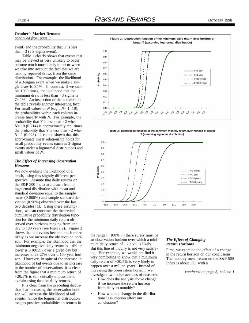
Figure 2: Distribution function of the minimum daily return over horizon of length T (assuming lognormal distribution)
0.0
0.1
0.2
0.3
0.4
0.5
0.6
0.7
0.8
0.9
1.0
-10.0 -9
.0-8
.0-7
.0-6
.0-5
.0-4
.0-3
.0-2
.0-1
.0 0.0 1.0 2.0 3.0 4.0 5.0 6.0 7.0 8.0 9.0
Pro
bab
ility
T=1 day
T=1 year
T=10 years
T=100 years
Figure 3: Distribution function of the minimum monthly return over horizon of length T (assuming lognomal distribution)
0.0
0.1
0.2
0.3
0.4
0.5
0.6
0.7
0.8
0.9
1.0
-25.0 -20.0 -15.0 -10.0 -5.0 0.0 5.0 10.0 15.0 20.0
Pro
bab
ility
T=1 month
T=1 year
T=10 years
T=100 years
PAGE 4 RISKS AND REWARDS OCTOBER 1998
October’s Market Demonscontinued from page 3
event) and the probability that Y is lessthan 3 (a 3-sigma event).
Table 1 clearly shows that events thatmay be viewed as very unlikely to occurbecome much more likely to occur whenwe take into account the fact that we aremaking repeated draws from the samedistribution. For example, the likelihoodof a 3-sigma event when we make a sin-gle draw is 0.1%. In contrast, if we sam-ple 1000 times, the likelihood that theminimum draw is less than 3 sigma is74.1%. An inspection of the numbers inthe table reveals another interesting fact:For small values of N (e.g., N=1, 10),the probabilities within each column in-crease linearly with N. For example, theprobability that Y is less than 2 whenN=10 (0.214) is approximately ten timesthe probability that Y is less than 2 whenN=1 (0.023). It can be shown that thisapproximate linear relationship holds forsmall probability events (such as 2-sigmaevents under a lognormal distribution) andsmall values of N.
The Effect of Increasing ObservationHorizonsWe now evaluate the likelihood of acrash, using this slightly different per-spective. Assume that daily returns onthe S&P 500 Index are drawn from alognormal distribution with mean andstandard deviation equal to the samplemean (0.066%) and sample standard de-viation (0.96%) observed over the lasttwo decades [1]. Using these assump-tions, we can construct the theoreticalcumulative probability distribution func-tion for the minimum daily return ob-served over horizons ranging from oneday to 100 years (see Figure 2). Figure 2shows that tail events become much morelikely as we increase the observation hori-zon. For example, the likelihood that theminimum negative daily return is 4% orlower is 0.0012% over a given day butincreases to 26.27% over a 100-year hori-zon. However, in spite of the increase inlikelihood of tail events due to an increasein the number of observations, it is clearfrom the figure that a minimum return of
20.5% is still virtually impossible toexplain using data on daily returns.
It is clear from the preceding discus-sion that increasing the observation hori-zon will increase the likelihood of tailevents. Since the lognormal distributionassigns positive probabilities to returns in
the range ( 100% ) there surely must bean observation horizon over which a mini- The Effect of Changing mum daily return of 20.5% is likely. Return HorizonsBut this line of inquiry is not very satisfy-ing. For example, we would not find itvery comforting to know that a minimumdaily return of 20.5% is very likely tohappen over a million years! Instead ofincreasing the observation horizon, weinvestigate two other avenues of research:
How does the analysis above changeif we increase the return horizonfrom daily to monthly?How would a change in the distribu-tional assumption affect ourconclusions?
First, we examine the effect of a changein the return horizon on our conclusions. The monthly mean return on the S&P 500Index is about 1%, with a
continued on page 5, column 1

Figure 4: Distribution function of the minimum daily return over horizon of length T (assuming t-distribution with 5 df)
0.0
0.1
0.2
0.3
0.4
0.5
0.6
0.7
0.8
0.9
1.0
-25.0 -20.0 -15.0 -10.0 -5.0 0.0 5.0 10.0 15.0 20.0
Pro
bab
ility T=1 day
T=1 year
T=10 years
T=100 years
Figure 5: Distribution function of the minimum daily return over horizon of length T (assuming t-distribution with 3 df)
0.0
0.1
0.2
0.3
0.4
0.5
0.6
0.7
0.8
0.9
1.0
-25.0 -20.0 -15.0 -10.0 -5.0 0.0 5.0 10.0 15.0 20.0
Pro
bab
ility T=1 day
T=1 year
T=10 years
T=100 years
vv 2
.
vv
v 2
½
vr
OCTOBER 1998 RISKS AND REWARDS PAGE 5
October’s Market Demonscontinued from page 4
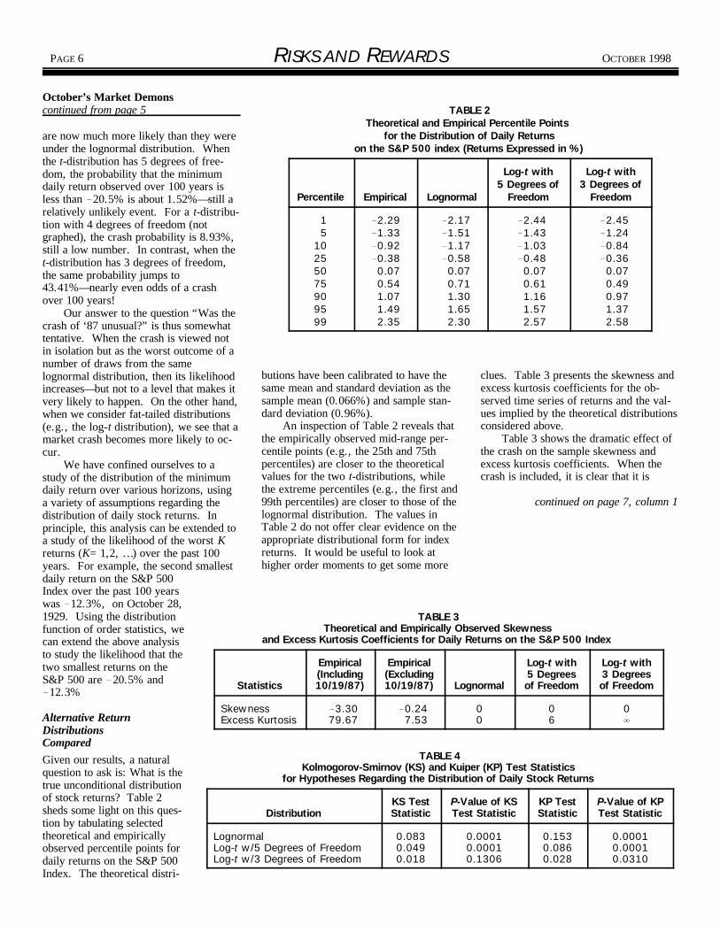
standard deviation of about 4%. Usingthese statistics, Figure 3 graphs the cumu-lative probability distribution function forthe minimum monthly return over obser-vation horizons ranging from one monthto 100 years. The probability that theminimum monthly return over a 100-yearobservation period is less than 21.5%(which was the return on the S&P 500Index over the month of October 1987) isapproximately 0.0067%. These numberssuggest that even when we look atmonthly returns, the market crash repre-sents a very unlikely event.
The Effect of Changing Distribution As-sumptionsNext we examine the effect of a change inthe distributional assumption on our re-sults. It is well-known that the uncondi-tional distribution of stock returns is char-acterized by the presence of fat tails. Adirect implication of this is that tail eventsare more likely than the lognormal distri-bution would predict. This line of inquiryhas a long history. Fama [2] concludedthat stock returns appeared to be drawnfrom a member of the stable Paretianfamily of distributions with infinite vari-ance. The normal distribution belongs tothe stable Paretian class and is the onlymember of this class with finite variance. Subsequent researchers have shown that ifthe time series of market returns is drawnfrom normal distributions withtime-varying variances, then the uncondi-tional distribution of market returnswould have fat tails.
One popular alternative to thelognormal assumption is to assume thatthe unconditional distribution of stockreturns is log-t. The log-t distributionarises when stock returns for each periodare lognormally distributed, with eachperiod’s variance being drawn from aninverted gamma distribution. If a randomvariable U has a log-t distribution with vdegrees of freedom, then log (U) t ,vwhere t follows a t-distribution with vvdegrees of freedom. The expected valueof log (U) is zero, and the variance of log(U) is equal to:
Let: .
Let r denote the log of 1 plus the rate of are infinite. (Note that in the latter casereturn on the market. The mean and the distribution has infinite kurtosis.)standard deviation of r are denoted by Figures 4 and 5 display the cumula-and respectively. tive probability distribution function for
In our study, we assume that: the minimum daily return for observation
.
follows a t-distribution with v degrees offreedom. We will present results for thecases v=5 and v=3. A point worth not-ing about t-distributions is that all evenmoments of orders equal to or greaterthan the v moment are infinite. So, forth
example, when v=5, even moments oforder 6 and above are infinite; and when
v=3, even moments of order 4 and above
horizons ranging from one day to 100years for v=5 and v=3, respectively. Anexamination of the graphs reveals that, asanticipated, tail events
continued on page 6, column 1
PAGE 6 RISKS AND REWARDS OCTOBER 1998
TABLE 2Theoretical and Empirical Percentile Points
for the Distribution of Daily Returnson the S&P 500 index (Returns Expressed in %)
Percentile Empirical Lognormal
Log-t with5 Degrees of
Freedom
Log-t with3 Degrees of
Freedom
15
10255075909599
2.291.330.920.380.070.541.071.492.35
2.171.511.170.580.070.711.301.652.30
2.441.431.030.480.070.611.161.572.57
2.451.240.840.360.070.490.971.372.58
TABLE 3Theoretical and Empirically Observed Skewness
and Excess Kurtosis Coefficients for Daily Returns on the S&P 500 Index
Statistics
Empirical(Including10/19/87)
Empirical(Excluding10/19/87) Lognormal
Log-t with5 Degreesof Freedom
Log-t with3 Degreesof Freedom
SkewnessExcess Kurtosis
3.3079.67
0.247.53
00
06
0
TABLE 4Kolmogorov-Smirnov (KS) and Kuiper (KP) Test Statistics
for Hypotheses Regarding the Distribution of Daily Stock Returns
DistributionKS TestStatistic
P-Value of KSTest Statistic
KP TestStatistic
P-Value of KPTest Statistic
LognormalLog-t w/5 Degrees of FreedomLog-t w/3 Degrees of Freedom
0.0830.0490.018
0.00010.00010.1306
0.1530.0860.028
0.00010.00010.0310
October’s Market Demonscontinued from page 5
are now much more likely than they wereunder the lognormal distribution. Whenthe t-distribution has 5 degrees of free-dom, the probability that the minimumdaily return observed over 100 years isless than 20.5% is about 1.52%—still arelatively unlikely event. For a t-distribu-tion with 4 degrees of freedom (notgraphed), the crash probability is 8.93%,still a low number. In contrast, when thet-distribution has 3 degrees of freedom,the same probability jumps to43.41%—nearly even odds of a crashover 100 years!
Our answer to the question “Was thecrash of ‘87 unusual?” is thus somewhattentative. When the crash is viewed notin isolation but as the worst outcome of anumber of draws from the samelognormal distribution, then its likelihoodincreases—but not to a level that makes itvery likely to happen. On the other hand,when we consider fat-tailed distributions(e.g., the log-t distribution), we see that amarket crash becomes more likely to oc-cur.
We have confined ourselves to astudy of the distribution of the minimumdaily return over various horizons, usinga variety of assumptions regarding thedistribution of daily stock returns. Inprinciple, this analysis can be extended toa study of the likelihood of the worst Kreturns (K=1,2, …) over the past 100years. For example, the second smallestdaily return on the S&P 500Index over the past 100 yearswas 12.3%, on October 28,1929. Using the distributionfunction of order statistics, wecan extend the above analysisto study the likelihood that thetwo smallest returns on theS&P 500 are 20.5% and
12.3%
Alternative Return Distributions ComparedGiven our results, a naturalquestion to ask is: What is thetrue unconditional distributionof stock returns? Table 2sheds some light on this ques-tion by tabulating selectedtheoretical and empiricallyobserved percentile points fordaily returns on the S&P 500Index. The theoretical distri-
butions have been calibrated to have the clues. Table 3 presents the skewness andsame mean and standard deviation as the excess kurtosis coefficients for the ob-sample mean (0.066%) and sample stan- served time series of returns and the val-dard deviation (0.96%). ues implied by the theoretical distributions
An inspection of Table 2 reveals that considered above.the empirically observed mid-range per- Table 3 shows the dramatic effect ofcentile points (e.g., the 25th and 75th the crash on the sample skewness andpercentiles) are closer to the theoretical excess kurtosis coefficients. When thevalues for the two t-distributions, while crash is included, it is clear that it is the extreme percentiles (e.g., the first and99th percentiles) are closer to those of the continued on page 7, column 1lognormal distribution. The values inTable 2 do not offer clear evidence on theappropriate distributional form for indexreturns. It would be useful to look athigher order moments to get some more

OCTOBER 1998 RISKS AND REWARDS PAGE 7
TABLE 5Daily GARCH-Forecast-Standardized Residuals
for the Days Surrounding the October 1987 Crash
Date
Return onS&P 500 Index
(%)
GARCH-PredictedStandard Deviation
(%)
GARCH-Forecast-Standardized
Residual
10/13/8710/14/8710/15/8710/16/8710/19/87
1.662.952.345.16
20.47
1.061.081.201.251.55
1.512.782.014.17
13.25
10/20/8710/21/8710/22/8710/23/8710/26/87
5.339.103.920.018.28
4.014.044.284.254.15
1.312.240.930.022.01
TABLE 6Monthly GARCH-Forecast-Standardized Residuals
for the Months Surrounding the Crash in October 1987
Month
Return onS&P 500 Index
(%)
GARCH-PredictedStandard Deviation
(%)
GARCH-Forecast-Standardized
Residual
September 1987October 1987November 1987December 1987
2.2021.528.167.35
4.364.347.416.93
0.755.201.250.91
October Market Demonscontinued from page 6
difficult to reconcile the sample higherorder moments with the theoretical mo-ments of any single distribution consid-ered above. On the other hand, when thecrash is excluded, the log-t distributionwith 5 degrees of freedom appears tohave predicted moments that match theempirically observed moments closely. However, since the crash did occur, it isdebatable whether it should be droppedfrom the analysis simply because it repre-sents an inconvenient data point!
We now turn to more formal tests ofthe distribution of daily stock re-turns—namely, the Kolmogorov- Smirnovtest and the Kuiper test. Table 4 presentsthe test statistics and the associated signif-icance levels.
The test statistics in Table 4 stronglyreject the null hypotheses that daily re-turns arise from a lognormal distributionor from a log-t distribution with 5 degreesof freedom. The null hypothesis of log-twith 3 degrees of freedom fails to be re-jected by both tests at the 1% level but isrejected by the Kuiper test at the 5%level. The results of the formal tests arethus consistent with our earlier findingsand strongly suggest that the uncondi-tional distribution of daily returns isfat-tailed with very large (possibly infi-nite) higher-order moments.
II. GARCH Forecasts AroundPeriods of Extreme MarketMovements
In Part I of this article we studied the un-conditional distribution of stock returnsover the last 100 years with special focuson the likelihood of a market crash. Ourconclusion was that a market crash hasnearly even odds of occurring over a pe-riod of 100 years if the unconditional dis-tribution of daily stock returns arisesfrom a fat-tailed distribution with verylarge (possibly infinite) higher-order mo-ments. It has been widely documentedthat such an unconditional distribution isconsistent with each period’s returns be-ing conditionally lognormally distributedwith time-varying conditional variances. In this section, we focus on a particularparameterization of the conditional vari-ance structure—namely, the GARCH(1,1) model—and study the behavior of
this model around periods of extreme had been about a week before themarket movements. crash.
GARCH Applied to October 1987To perform this study, we estimated sepa-rate GARCH(1,1) models using daily and ber 19, 1987, in contrast to themonthly returns on the S&P 500 Index. 20-sigma characterization of theThe daily model was estimated using re- crash using unconditional moments ofturns over the period March 1980 through the distribution of daily returns.September 1987 (1,906 days), and themonthly model used data from January1973 through September 1987 (177months). Table 5 presents theGARCH-forecast- standardized residuals and other numbersof interest for the days surrounding thecrash in October 1987. As the estimationperiod for the models excluded October1987, our reported results areout-of-sample.
Table 5 documents a number of in-teresting facts:
In response to sharp market moves inthe days immediately preceding thecrash, the GARCH forecast of thestandard deviation for October 19,1987, was about 50% higher than it
The crash return constitutes a13-sigma event relative to theGARCH forecast volatility for Octo-
After the crash, GARCH forecastvolatility rises to a level of over 4%per day, which causes many of thesharp post-crash market movementsto be classified as “normal” eventsthat are plausible even if daily returnsare conditionally lognormally distrib-uted.A look at the time series of GARCH
forecasts shows that the predicted volatil-ity continues to be very high for severalweeks after the crash. For example, thedaily GARCH forecast as of the end ofDecember 1987 (using data through De-cember 1987 to estimate
continued on page 8, column 1

Figure 6: S&P500 level and SPX-option-implied volatility over the last one year
13.0
14.0
15.0
16.0
17.0
18.0
19.0
20.0
21.0
22.0
7/1/96 8/1/96 9/1/96 10/1/96 11/1/96 12/1/96 1/1/97 2/1/97 3/1/97 4/1/97 5/1/97 6/1/97 7/1/97
Date
Imp
lied
vo
lati
lity
(SP
X o
pti
on
s)
600
650
700
750
800
850
900
S&
P50
0 le
vel
Implied volatility (SPX options)
S&P500 level
PAGE 8 RISKS AND REWARDS OCTOBER 1998
October Market Demonscontinued from page 7
the GARCH parameters) was 1.60%—anumber that is about 50% higher thanpre-crash forecasts. This is a manifesta-tion of the well-known high degree ofpersistence in daily GARCH forecasts. Table 6 shows GARCH-standardized re-siduals using the monthly GARCHmodel. The monthly GARCH forecastsalso rise sharply following the month ofthe crash and continue to remain high fora few months after the crash.
The fundamental intuition built intoGARCH models is the notion of volatilityclustering—i.e., periods of high volatilityare likely to be followed by more periodsof high volatility. If historical volatility islow, then GARCH models will continueto forecast low volatility. Although“outliers” are not ruled out even whenusing GARCH forecasts, the distinguish-ing feature of an accurate GARCH modelis that these outliers would be randomlydistributed in time, in contrast to the fore-casts of naïve models where outlierswould appear clustered together. Judgedby this metric, Tables 5 and 6 provideanecdotal evidence that, although thecrash itself appears as an outlier,GARCH models are at least partially suc-cessful in explaining the sharp movementsaround the period of the market crash.
Can We Predict an Abrupt Market Tran-sition?Since GARCH models use a weightedaverage of historical realized volatility topredict future volatility, in times of atransition from a low-volatility regime toa high-volatility regime the first few sharpmovements may appear as outliers thatare unanticipated by the GARCH model. An interesting question we might ask is:Are there other techniques that might beused to predict extreme market move-ments? This question is of clear interestin the current regime since popular debatein the weeks leading up to October 27,1997, centered on comparisons with Oc-tober 1987 and on the likelihood of an-other market crash.
One obvious answer is to look atS&P 500 Index option-implied volatilityforecasts. Figure 6 shows the time-seriesevolution of the S&P 500 Index level overthe past one year and the S&P 500 Index(SPX) option-implied volatility at the be-ginning of each month from July 1996through July 1997. The annualized aver-age implied volatility using near-term
(less than one month to maturity), In summary, our study of GARCH-near-the-money options has risen from standardized residuals around the periodapproximately 13.29% on July 1, 1996, of the crash of October 1987 shows that,to about 20.25% on July 1, 1997. Over while the crash itself was an outlier, mostthe same time period, the S&P 500 Index of the market volatility subsequent to thehas risen from 670 to 885. Somewhat crash can be fully accounted for usingsurprisingly, over a number of months GARCH forecasts. GARCH models use(e.g., May and June 1997) increases in the presence or absence of outliers to pre-the S&P 500 Index have been accompa- dict subsequent increases or decreases innied by increases in option-implied vola- volatility. Hence, while outliers may ex-tility, an observation which is at odds ist even when using GARCH forecasts,with the “leverage effect” (i.e., the usu- these outliers are likely to be randomlyally negative relationship between price dispersed through time. In the currentmovements and volatility). regime, we saw that option-implied vola-
One explanation for Figure 6 is that tility as of July 1, 1997, appeared to beoptions market participants expected the much higher than GARCH forecasts. S&P 500 Index to have higher short-term One explanation for this finding is thatvolatility in the coming weeks and options market participants expected tomonths. In contrast to the high implied see higher volatility in the comingvolatility forecasts, the conditional vari- weeks/months for the S&P 500 Index. ance prediction of GARCH models ranges Since the expected increase in volatilityfrom approximately 14.10% as of July 1, has been realized, we would expect that1996, to approximately 15.55% as of July GARCH forecasts will also respond.1, 1997. Since the sharp movements thatwere anticipated by options market partic-ipants were realized in October 1997, wewould expect that GARCH forecastswould have also risen subsequent to thefirst few sharp movements in the market.
Our study of option-implied volatilityover the past one year suggests that wecan incorporate “forward-looking” infor-mation in volatility forecasts by combin-ing option-implied volatility with GARCHforecasts. For example, we could esti-mate a GARCH model using op-tion-implied volatility as one of the vari-ables in the conditional variance equation. Studies by Day and Lewis [3] andLamoureux and Lastrapes [4] suggest thatthese two sources of information are com-plementary.
III. Impact of the Crash onBacktesting and PerformanceEvaluation
In the previous sections we have studiedissues relating to the likelihood of a crash(unconditional study) and the behavior ofGARCH forecasts of the S&P 500 Indexvolatility around the period of the crash(conditional study). In this section, weprovide some thoughts on
continued on page 9, column 1

Figure 7: Annualized Sharpe ratio for S&P500 index (over various horizons) including and excluding October 1987
0
0.2
0.4
0.6
0.8
1
1.2
1.4
1.6
01/1987-12/1987 01/1986-12/1990 01/1986-12/1995 01/1976-12/1995
Horizon
Annualized SR (including Oct 87)
Annualized SR (excluding Oct 87)
ˆ,B2,t
p,A,t
fB,t
2 BTˆ,B2,t
gB,t IC rB,t mB s 1 IC 2ut
OCTOBER 1998 RISKS AND REWARDS PAGE 9
October Market Demonscontinued from page 8
the influence of the crash on backtestinginvestment strategies and on performanceevaluation.
The Importance of Time Period ChoiceThe first point to note is that the time ho-rizon over which backtesting and/or per-formance evaluation are conducted willdetermine the extent to which excludingthe crash will affect the reported results. Figure 7 plots the ex-post Sharpe ratio onthe S&P 500 Index over horizons of 1, 5,10, and 20 years, including and excludingthe crash. As the horizon lengthens, wesee that the Sharpe ratio when the crash isincluded gradually approaches the Sharperatio excluding the crash. We shouldpoint out that because we need very largesample sizes to estimate mean returnsaccurately, the two sets of Sharpe ratiosare not statistically distinguishable fromone another (i.e., they are within twostandard errors of each other).
The second point is that excluding thecrash can have dramatic implications forthe profitability of certain types of strate-gies. For example, Sheikh [5] demon-strates that a strategy of buying the S&P500 Index plus writing out-of-the-moneyputs on the index was a profitable strategy(relative to buying the S&P 500 Index)over periods strictly before and strictlyafter the crash. The post-crash periodthat Sheikh studied was August 1988through February 1995. In contrast, asimilar strategy that was put in placestarting in September 1987 lagged thecumulative return on the S&P 500 Index,even after over seven years (as of Febru-ary 1995). In other words, the loss suf-fered in the month of the crash was morethan the gains made by the strategy overthe next seven years!
The third point is that it is a goodidea to run backtests over historical peri-ods that represent different regimes—e.g., bull and bear markets, periods oflow volatility and high volatility, etc. Figure 8 shows the cumulative return onthe S&P 500 Index over the 10-year pe-riod January 1987 through December1996. It is evident from the figure thatthere have not been too many badmonths, especially over the past fiveyears. The crash represents a useful ob-servation precisely because it was a par-ticularly bad month. Including this obser-vation in backtests serves as a check onthe robustness of proposed investment
strategies.
Should the Crash Be Included in Performance Studies?Finally, we consider performance evalua-tion in the presence of the crash. As theabove analysis of the Sharpe ratio sug-gests, the total risk/return picture, espe-cially over smaller horizons, differs sig-nificantly depending on whether or not thecrash is included in the sample. For anactive manager who is usually fully in-vested in equities, including the crashdoes not bias performance results sincethe active manager is evaluated based onhis or her active risk/return profile (i.e.,risk and return net of the market).
Let us consider the more difficultquestion of an active manager who aimsto achieve superior returns by forecastingthe returns on the S&P 500 Index (that is,by timing the market). Let r be theB,texcess return on the S&P 500 Index inperiod t and let denote the per-periodlong-run expected excess return on theindex. Each period, the market timer hasa forecast of the excess return on the in-dex over its long-run average. In sym-bols, for each period the market timer hasa forecast f of the value of r . LetB B,t B
denote the risk aversion coefficient ofBTthe investor for benchmark timing and let be the investor’s forecast of thevariance on the index over period t. Then, the optimal active beta position forthe investor is given by:
Grinold and Kahn [6] discuss the appro-priate objective function for an activemanager and derive the optimal activebeta policy stated above. We conducted asimulation study using the actual historyof realized market returns over the periodJanuary 1987 through December 1996. The market timer is assumed to makemonthly forecasts of the index return. Each month, the market timer receives asignal g as follows:B,t
IC = the information coefficient of themanager
m = the average excess return on theBindex over the 10-year sampleperiod
s = the sample standard deviation ofthe excess return on the index,and
u = a random number drawn from atdistribution with zero mean andunit standard deviation.
continued on page 10, column 1

Figure 8: Cumulative return on the S&P500 index since January 1st, 1987
0.5
1.0
1.5
2.0
2.5
3.0
3.5
4.0
4.5
Jan-87
Jul-87
Jan-88
Jul-88
Jan-89
Jul-89
Jan-90
Jul-90
Jan-91
Jul-91
Jan-92
Jul-92
Jan-93
Jul-93
Jan-94
Jul-94
Jan-95
Jul-95
Jan-96
Jul-96
Cumulative return on S&P500 index
ˆ,B2,t
fB,t E rB,t B gB,t (IC)gB,t
PAGE 10 RISKS AND REWARDS OCTOBER 1998
TABLE 7Ex-post Information Ratios (IR) for Market Timing
Over the Period January 1987 through December 1996(Average over 100 Simulations)
InformationCoefficient
Average Ex-post IR(including October 1987)
Average Ex-post IR(excluding October 1987)
0.050.100.15
0.1910.3960.467
0.1950.3770.448
October Market Demonscontinued from page 9
r = is set equal to the observed ex-B,tcess return on the S&P 500 In-dex in month t.
Given this signal, the manager con-structs an optimal forecast of the excessreturn on the index as follows:
For simplicity, we assume that theinvestor’s forecast of the variance of the
index return in month t, is equal tos for all months. For a given sequence2
of signal realizations, we can derive thecorresponding time series of active betapositions. Using the actual history ofmarket returns, we can then compute theex-post information ratio for the investor. We considered three different IC levels;0.05, 0.10, and 0.15. For each IC, weran 100 simulations of the entire 10-yearhistory from January 1987 through De-cember 1996. Table 7 reports the aver-age ex-post information ratios acrossthese simulations.
Table 7 shows that there are no sig-nificant differences between the two col-umns of information ratios. In otherwords, including the crash does not ap-pear to make a difference for the perfor-mance evaluation of a market timer.
SummaryIn this article, we have presented someperspectives on the crash of October1987. We found that the likelihood of amarket crash increases dramatically if theunconditional distribution of stock returnsis fat-tailed with very large (possibly infi-nite) higher-order moments. Our studyof GARCH forecasts showed that, withthe exception of the crash itself, theseforecasts were at least partially successfulin capturing sharp movements around theperiod of the crash. We found that op-
tion-implied volatility has increased dra- Index Options,” Journal of Econo-matically over the past one year, suggest- metrics, v.52, 1992, pp.267–287.ing that the market expects higher volatil-ity in the weeks/months ahead. Finally,we offered some thoughts on the impactof the crash on backtesting and perfor-mance evaluation. We showed via a sim-ulation study that including the month ofthe crash does not have a significant ef-fect on the ex-post information ratios of amarket timer.
End Notes1. Throughout this section, we assume
that the time series of daily returnsiid (independent and identically dis-tributed) draws from the specifiedunconditional distribution. In Part IIof this article we will explore thebehavior of conditional variancesaround the period of the crash.
2. Fama, Eugene F., “The Behavior ofStock Market Prices,” Journal ofBusiness, no. 38, 1995, pp.34–105.
3. Day, Theodore E. and Craig M.Lewis, “;Stock Market Volatility andthe Information Content of Stock
4. Lamoureux, Christopher and WilliamLastrapes, “Forecasting Stock ReturnVariance: Towards an Understandingof Stochastic Implied Volatility,” TheReview of Financial Studies, no. 6,1993, pp.293–326.
5. Sheikh, Aamir, “Portfolio Construc-tion with Derivatives,” BARRA’s19th Annual Equity Research Semi-nar, Pebble Beach, CA, June 11–14,1995.
6. Grinold, Richard C. and Ronald N.Kahn, Active Portfolio Management,Probus Publishing, Chicago, IL,1995.
Vinod Chandrashekaran is a Senior Con-sultant in the Research Group at BARRAInc. in Berkeley, California.

OCTOBER 1998 RISKS AND REWARDS PAGE 11
“The downfall of the Soviet Union in 1989 leadingto only one superpower, peace in the Middle East,positive demographics, and global capitalism mayhave lulled Joe and Lucy Public into believing thatnothing can go wrong.”
Taking Stock: No Pain No Gain, or What They Did Not Tell You about Goldilocks by Nino Boezio
f you haven’t heard it already, it’s When Goldilocks later awoke and saw the own destiny. For the latter, wealth gen-Itime that someone finally told you the first bear, she did not pay any attention to eration became the equivalent to investingcomplete story about Goldilocks and it. She was still hungry and thus went as much as one could in the stock market.the Three Bear Markets. back to eating soup, for now some of the The stock market, as it became in theGoldilocks is a soup connoisseur and hot ones cooled off (a buying opportu- 1920s (Japan in the 1980s), was increas-
loves to try various soups. The amount nity), not realizing that the circumstances ingly seen as the “no pain always gain”and variety of soups (equities) Goldilocks had now changed (Phase I of a bear mar- approach to increase one’s financial(today’s equity investors) eats depends on ket—denial). When the second bear ap- health. It would grant a person ultimatehow the temperature (the economy) of the pears (Phase II of a bear mar- financial independence (“deliverancesoup is—too hot, too cold, or just right. ket—realization), she may realize that from serfdom”) and allow one to retireThe soups overall were not much to her eating more soup in the presence of the early to a life of luxury. The downfall ofliking in the early 1990s because the tem- bears will put her in danger and her trepi- the Soviet Union in 1989 leading to onlyperature was “too cold” (recession), “too dation may result in her hunger being re- one superpower, peace in the Middlehot” in 1994 (economic overheating), but placed by hesitation and concern. She East, positive demographics, and global“just right“ in the last few years (hence will stop eating and the hot soups (equi- capitalism may have lulled Joe and Lucythe name Goldilocks economy). ties) will get even cooler (cheaper). Public into believing that nothing can go
While is search for soups, Goldilocks When the third bear appears (Phase III of wrong. Initially it was a good bet, untilhappened to enter into the lair of the bears a bear market— capitulation), she may too many began to believe it and drove
(overvaluation) but was not too concerned have not already done her harm, then they economy which potentially can suck upabout where she arrived. She had never probably will not do so and she should the excess supply of goods, the actions ofseen bears before and only heard rumors probably heat up the soups and start eat- this or that politician or leader, emergingof past rampages in foregone times. She ing once again. However, by then she Western Europe, or sometimes just sim-was told that bears these days are kept probably has run out and missed out on ply the use of money from one group toaway in zoos (the new era), and if one the soupfest (Phase I of a bull market) pay for the misgivings or “irrational exu-ever were to escape, the zookeepers that could ultimately ensue if she had only berance” of another group. As was(Alan Greenspan, the Fed, the stuck around longer. Or perhaps the pointed out in my article “It’s DifferentBundesbank, the International Monetary bears’ stove is broken (a depression) and This Time” in the March 1998 issue ofFund etc.) would quickly go after the bear she will not get a chance to eat more soup Risks and Rewards, traditional solutionsand put it back into captivity. Hence for a very long time. may not work this time, and the problemsthere was nothing to fear. She did not are substantially different than they ini-know that there were still bears running tially appear on the surface. It is nowfree. said that about 50% of the global econ-
The bears were not at home (lost all omy is in or on the verge of entering acredibility) when Goldilocks finally recession because of falling world de-showed up. Goldilocks, having tried the mand from the international financial cri-various soups, liked the ones that in her sis.opinion were not too hot or too cold, and It is sad to see a person’s hopesgorged herself. Needless to say, all that dashed or rattled as a result of any eating made her sleepy and she did nothear the rumblings outside (Asia, Russia, continued on page 28, column 1South America), sounds made by the re-turning bears. She went to sleep.
Since Goldilocks had never seen livebears, she did not know what to fear.
finally acknowledge valuations skyward all over the world.her plight and run for No one in the world communitycover (and will even wants to suffer pain, even though theirstart vomiting what behavior may at times create pain for oth-she has already ers and ultimately themselves. When theeaten), and all the pain comes, there is often a mad scramblesoups will become to find a “cure” rather than to accept thefreezingly cold. In hurt, learn from it, take the lumps, andthis latter phase, she move on. The cure in the economicshould probably real- world has become known as the Interna-ize that if the bears tional Monetary Fund, a strong U.S.
No Pain, No Gain: Understanding GoldilocksHumanity has been searching for the HolyGrail for thousands of years—in modern-day terminology this is called the “freelunch” (or should we call it the “freesoup”).
There has always been a quest by theaverage person to find the ultimate happi-ness in personal life, the perfect balancebetween recreation and work (for somethat would mean no work), and for suffi-cient wealth so that one may guide his
PAGE 12 RISKS AND REWARDS OCTOBER 1998
FIGURE 1Old-Age Dependency Ratio
in the United States
The Baby Boom, the Baby Bust, and Asset Markets by Timothy Cogley and Heather Royer
Editor’s Note: Reprinted from the these elements will be neces-Federal Reserve Bank of San Francisco sary to sustain the programs. Economic Letter, Number 98–20, June Because of doubts about26, 1998. The opinions expressed in this the future of Social Security, itarticle do not necessarily reflect the views may be prudent for householdsof the management of the Federal Reserve to prepare for retirement byBank of San Francisco, or of the Board of increasing their own personalGovernors of the Federal Reserve System. savings. Venti and Wise
n about 10 to 15 years, the first waveIof post-war baby boomers will beginto retire, and we will start to see alarge generational shift from young to
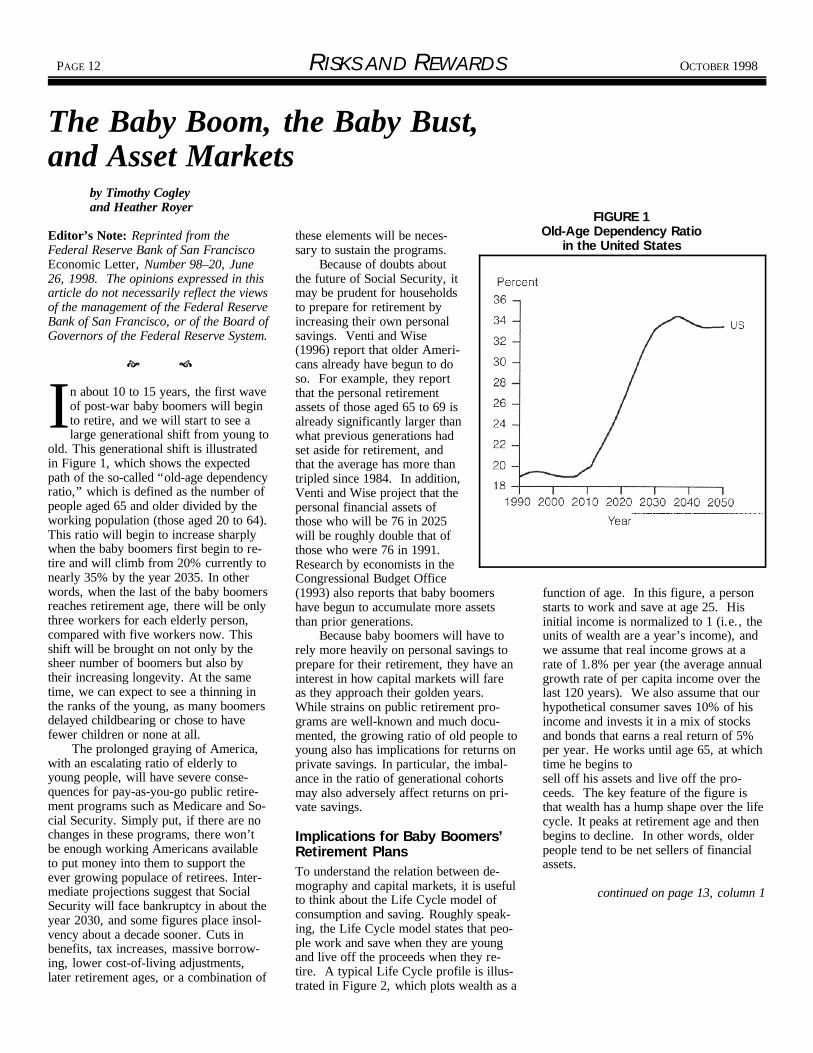
old. This generational shift is illustratedin Figure 1, which shows the expectedpath of the so-called “old-age dependencyratio,” which is defined as the number ofpeople aged 65 and older divided by theworking population (those aged 20 to 64). This ratio will begin to increase sharplywhen the baby boomers first begin to re-tire and will climb from 20% currently tonearly 35% by the year 2035. In otherwords, when the last of the baby boomersreaches retirement age, there will be onlythree workers for each elderly person,compared with five workers now. Thisshift will be brought on not only by thesheer number of boomers but also bytheir increasing longevity. At the sametime, we can expect to see a thinning inthe ranks of the young, as many boomersdelayed childbearing or chose to havefewer children or none at all.
The prolonged graying of America,with an escalating ratio of elderly toyoung people, will have severe conse-quences for pay-as-you-go public retire-ment programs such as Medicare and So-cial Security. Simply put, if there are nochanges in these programs, there won’tbe enough working Americans availableto put money into them to support theever growing populace of retirees. Inter-mediate projections suggest that SocialSecurity will face bankruptcy in about theyear 2030, and some figures place insol-vency about a decade sooner. Cuts inbenefits, tax increases, massive borrow-ing, lower cost-of-living adjustments,later retirement ages, or a combination of
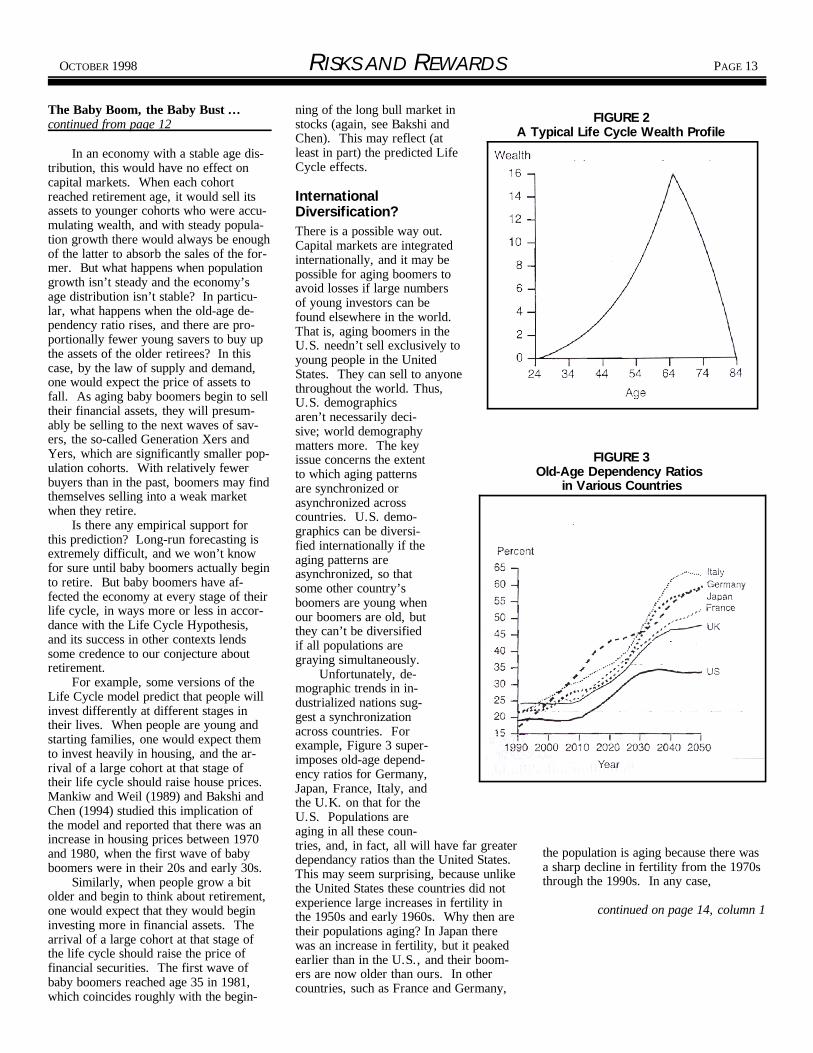
(1996) report that older Ameri-cans already have begun to doso. For example, they reportthat the personal retirementassets of those aged 65 to 69 isalready significantly larger thanwhat previous generations hadset aside for retirement, andthat the average has more thantripled since 1984. In addition,Venti and Wise project that thepersonal financial assets ofthose who will be 76 in 2025will be roughly double that ofthose who were 76 in 1991. Research by economists in theCongressional Budget Office(1993) also reports that baby boomers function of age. In this figure, a personhave begun to accumulate more assets starts to work and save at age 25. Histhan prior generations. initial income is normalized to 1 (i.e., the
Because baby boomers will have to units of wealth are a year’s income), andrely more heavily on personal savings to we assume that real income grows at aprepare for their retirement, they have an rate of 1.8% per year (the average annualinterest in how capital markets will fare growth rate of per capita income over theas they approach their golden years. last 120 years). We also assume that ourWhile strains on public retirement pro- hypothetical consumer saves 10% of hisgrams are well-known and much docu- income and invests it in a mix of stocksmented, the growing ratio of old people to and bonds that earns a real return of 5%young also has implications for returns on per year. He works until age 65, at whichprivate savings. In particular, the imbal- time he begins toance in the ratio of generational cohorts sell off his assets and live off the pro-may also adversely affect returns on pri- ceeds. The key feature of the figure isvate savings. that wealth has a hump shape over the life
Implications for Baby Boomers’Retirement PlansTo understand the relation between de-mography and capital markets, it is usefulto think about the Life Cycle model ofconsumption and saving. Roughly speak-ing, the Life Cycle model states that peo-ple work and save when they are youngand live off the proceeds when they re-tire. A typical Life Cycle profile is illus-trated in Figure 2, which plots wealth as a
cycle. It peaks at retirement age and thenbegins to decline. In other words, olderpeople tend to be net sellers of financialassets.
continued on page 13, column 1
OCTOBER 1998 RISKS AND REWARDS PAGE 13
FIGURE 2A Typical Life Cycle Wealth Profile
FIGURE 3Old-Age Dependency Ratios
in Various Countries
The Baby Boom, the Baby Bust ... ning of the long bull market incontinued from page 12 stocks (again, see Bakshi and
In an economy with a stable age dis-tribution, this would have no effect oncapital markets. When each cohortreached retirement age, it would sell itsassets to younger cohorts who were accu-mulating wealth, and with steady popula-tion growth there would always be enoughof the latter to absorb the sales of the for-mer. But what happens when populationgrowth isn’t steady and the economy’sage distribution isn’t stable? In particu-lar, what happens when the old-age de-pendency ratio rises, and there are pro-portionally fewer young savers to buy upthe assets of the older retirees? In thiscase, by the law of supply and demand,one would expect the price of assets tofall. As aging baby boomers begin to selltheir financial assets, they will presum-ably be selling to the next waves of sav-ers, the so-called Generation Xers andYers, which are significantly smaller pop-ulation cohorts. With relatively fewerbuyers than in the past, boomers may findthemselves selling into a weak marketwhen they retire.
Is there any empirical support forthis prediction? Long-run forecasting isextremely difficult, and we won’t knowfor sure until baby boomers actually beginto retire. But baby boomers have af-fected the economy at every stage of theirlife cycle, in ways more or less in accor-dance with the Life Cycle Hypothesis,and its success in other contexts lendssome credence to our conjecture aboutretirement.
For example, some versions of theLife Cycle model predict that people willinvest differently at different stages intheir lives. When people are young andstarting families, one would expect themto invest heavily in housing, and the ar-rival of a large cohort at that stage oftheir life cycle should raise house prices.Mankiw and Weil (1989) and Bakshi andChen (1994) studied this implication ofthe model and reported that there was anincrease in housing prices between 1970and 1980, when the first wave of babyboomers were in their 20s and early 30s.
Similarly, when people grow a bitolder and begin to think about retirement,one would expect that they would begininvesting more in financial assets. Thearrival of a large cohort at that stage ofthe life cycle should raise the price offinancial securities. The first wave ofbaby boomers reached age 35 in 1981,which coincides roughly with the begin-
Chen). This may reflect (atleast in part) the predicted LifeCycle effects.
International Diversification?There is a possible way out.Capital markets are integratedinternationally, and it may bepossible for aging boomers toavoid losses if large numbersof young investors can befound elsewhere in the world. That is, aging boomers in theU.S. needn’t sell exclusively toyoung people in the UnitedStates. They can sell to anyonethroughout the world. Thus,U.S. demographicsaren’t necessarily deci-sive; world demographymatters more. The keyissue concerns the extentto which aging patternsare synchronized orasynchronized acrosscountries. U.S. demo-graphics can be diversi-fied internationally if theaging patterns areasynchronized, so thatsome other country’sboomers are young whenour boomers are old, butthey can’t be diversifiedif all populations aregraying simultaneously.
Unfortunately, de-mographic trends in in-dustrialized nations sug-gest a synchronizationacross countries. Forexample, Figure 3 super-imposes old-age depend-ency ratios for Germany,Japan, France, Italy, andthe U.K. on that for theU.S. Populations areaging in all these coun-tries, and, in fact, all will have far greaterdependancy ratios than the United States. This may seem surprising, because unlikethe United States these countries did notexperience large increases in fertility inthe 1950s and early 1960s. Why then aretheir populations aging? In Japan therewas an increase in fertility, but it peakedearlier than in the U.S., and their boom-ers are now older than ours. In othercountries, such as France and Germany,
the population is aging because there wasa sharp decline in fertility from the 1970sthrough the 1990s. In any case,
continued on page 14, column 1
PAGE 14 RISKS AND REWARDS OCTOBER 1998
The Baby Boom, the Baby Bust ...continued from page 13
because the demographic profiles are syn- well, in ways we are just beginning tochronized, it seems unlikely that investors explore.in these countries will be net buyers ofcapital when aging Americans begin to Timothy Cogley, Senior Economistsell. If anything, this figure suggests that Heather Royer, Research Associateinternational linkages among developedcountries are likely to amplify life cycleeffects in the United States.
What about developing countries? Demographers project that their old-agedependency ratios will also rise, but ex-pect the increase to occur roughly 50years later than in the industrializedworld. Since their demographic profilesdiffer from the developed world’s, per-haps aging boomers in the latter can sellto younger boomers in the former. Butwill they have the means to buy? Capitaltends to be scarce in developing coun-tries, and unless they can grow rich in thenext 25 years, it seems unlikely that theywill be in a position to become net lendersto the developed world.
Other ConsiderationsThe looming crunch might be slightlyeased under several scenarios. For exam-ple, educated baby boomers may chooseto stay in their careers longer, workingpast the traditional age of retirement; theyneed not sell their assets if they earn steady paychecks. In addition, the periodover which the Baby Boom generation is 1994. “Baby Boom, Population Ag-expected to retire spans about 30 years. ing, and Capital Markets.” JournalCapital markets might have time to adjust of Business 67, pp. 165–202.to the gradual decline in supply of fundsfor capital investment. For example, ifGen-Xers, Yers, and Zers were to antici-pate further cuts in Social Security bene-fits, they might save a higher fraction oftheir incomes, and this would compensatefor the fact that there are relatively few ofthem. Despite such possibilities, thesurging old-age dependency ratio remainsa significant generational challenge, notjust for Social Security, but perhaps forprivate retirement plans as
REFERENCES
Bakshi, Gurdip S., and Zhiwu Chen.
Congressional Budget Office. 1993.“Baby Boomers in Retirement: AnEarly Perspective.”
Mankiw, N. Gregory, and David Weil.1989. “The Baby Boom, the BabyBust, and the Housing Market.” Re-gional Science and Urban Economics19, pp. 235–258.
Venti, Steven F., and David A. Wise.1996. “The Wealth of Cohorts: Re-tirement Saving and the ChangingAssets of Older Americans.” NBERWorking Paper No. 5609.
Subjective Value at Risk by Glyn Holton
Editor’s Note: The following article orig- If the VaR revolution is to succeed, it hind the screen, the man sees the result ofinally appeared in the August 1997 issue must be tempered by such concerns. Af- the die toss, but you have not yet seen it. of Financial Engineering News and is ter all, VaR is only a tool. All tools have In this example, the outcome is certain. reprinted with permission. limitations. For example, a hammer can It has already been determined. Uncer-
alue-at-Risk (VaR) is becomingVsomewhat of a revolution. Around the globe, organizationsare racing to implement the new
technology. Pundits propose extendingVaR to other risks, including credit riskand operational risk [1]. Some even sup-pose that all the risks of an organizationshould be summarized with a single riskmeasure [2].
It is the nature of revolutions thatthere be a backlash. One has begun. Critics suggest that VaR may be ineffec-tive for assessing risks other than marketrisks [3]—or that it fails even with marketrisk [4]. Others have noted disturbinginconsistencies between risk estimatesproduced by different implementations ofVaR [5].
drive nails, but it cannot drive screws. tainty exists only in your head—but theSaying that the hammer is limited is dif- risk is real until you see the die.ferent from saying it is flawed. Let’s try to quantify your risk in this
To understand the limits of VaR, we example. To characterize the risk, weneed to explore what it means to “quan- need to describe the uncertainty as well astify” risk. Let’s start by defining risk. your exposure to that uncertainty. Obvi-Risk is exposure to uncertainty. Accord- ously, your exposure is $100. That is theingly, risk has two components: (1) un- amount you stand to lose. But what iscertainty; and (2) exposure to that uncer- your uncertainty— what is the probabilitytainty. that you will lose $100?
A synonym for uncertainty is igno- If you say it is one chance in six, Irance. We face risk because we are igno- am sorry. You are wrong. I forgot torant about the future—after all, if we mention that the die is 10-sided. Thiswere omniscient, there would be no risk. illustrates an important point. WheneverBecause ignorance is a personal experi- we try to quantify risk, we are describingence, risk is necessarily subjective. our own understanding of a situation. When we put a number on risk, that num- Often, there will be aspects ber says as much about us—how little weknow—as it says about the world around continued on page 15, column 1us.
Suppose you are in a casino. A manrolls a die behind a screen. If the resultis a 6, you are going to lose $100. Be-

OCTOBER 1998 RISKS AND REWARDS PAGE 15
Subjective Value at Riskcontinued from page 14
of a situation that we are simply unaware her risk limit. She knows the markets would reduce the risk manager to being,of. It is one thing to not know the answer and is aware of a combination of market in effect, just another trader.to a question. It is another matter to not factors—perhaps central banks are inter- Instead, we implement an objectiveeven know the question exists. vening in the markets—that are going to benchmark for risk in the form of a VaR
Returning to our casino example, we drive the yen up in the short-term. She model. It may assume that market vari-still don’t know your probability of losing considers the position appropriate. ables are normally distributed despite$100. It is not one in ten. After all, the Her risk manager disagrees. He some observers preferring the lognormalman throwing the die may be cheating. doesn’t know about central bank inter- assumption. It may not capture marketWe are aware of the possibility, but it is vention—and he doesn’t care. All he leptokurtosis. It probably won’t under-difficult to place a number on that risk. knows is that the trader has exceeded her stand “sticky” volatilities. This is not
Would it help if I told you the man is limit, and he calls her on it. important.unshaven and smells of whiskey? Maybe Reviewing the VaR number that indi- If we have a perfect model, it wouldyour opinion would change if I told you cates her limit violation, the trader re- know everything there was to know aboutinstead that he is a kindly grandfather torts: “The model is wrong. I know the the markets. It would eliminate the needwearing a boy scout cap. Changing the markets. I know what the central banks for traders. We could trade the portfoliodescription may sway some peoples’ are doing. I’m on the phone with FX based upon the model—and we would beopinions. It may not sway others’. Risk professionals all day long. This VaR foolish not to.is subjective. model is just a bunch of formulas. It A VaR model, however, is limited
So what does this mean if we want to doesn’t know the yen is going up, but I because it is objective whereas risk takingmeasure the financial risks of an organi- do. There is zero risk in my long posi- is subjective. If we deny that subjectiv-zation? To find out, let’s look at how tion because any other market position, ity, we deny a role for human judgment. risks are quantified. It is a four-step pro- under these circumstances, would be ri- Rather than trade portfolios based upon acess: diculous.” model, we rely upon traders because we
Who is right, and who is wrong? believe they understand things the modelDefine the risk to be measuredAgree on a model for that riskSpecify a risk measure that is com-patible with that modelEstimate the value of that measureimplied by the model.For example, the process might be as
follows:Risk: market risk of a specified port-folioRisk model: market variables areassumed to be jointly normally dis-tributed with specified volatilities andcorrelationsRisk measure: one-day 90% VaRRisk estimate: achieved with MonteCarol simulation using 5,000 quasi-randomly generated scenarios.It is the second step of the process
that is pivotal. It is at this point that wetake the subjective notion risk and de-scribe it in an objective manner. How-ever, a group of individuals may agree ona model, but retain their own subjectiveopinions about the risk. In this sense, themodel does not make risk an objectivenotion, it merely makes the measure ofrisk an objective notion.
Let’s continue with the example ofmarket risk. Suppose a trading operationhas implemented the above VaR system. One day a trader takes on a sizable longposition in the Japanese yen, exceeding
The trader knows the markets. It’s her cannot.job. By the same token, what is the point This leaves us with two—potentiallyin having a risk manager who is going to inconsistent—market views: that of thebe overruled by every trader with a mar- model; and that of the traders.ket view? The question is: How can we use the
Some might perceive that the answer objective VaR model to manage the risk-is to build a better VaR model— one that taking process, but not place arbitrary—orsomehow captures the trader’s intuitive even dangerous—restrictions upon theunderstanding of central bank interven- activities of traders?tion. Others may cling to the existing The answer is risk limits. TheseVaR model, claiming that efficient mar- represent explicit authority for traders tokets and no-arbitrage conditions ensure its take positions that differ from the model’sultimate validity. perception of the markets. Risk limits
In fact, neither approach can possibly enable an organization to manage risk bywork. They both make a supposition that limiting traders to taking positions withinthere is a “right” model—if only we can a specified range. The role of the VaRidentify it. Markets, however, are too model is to objectively define what thatcomplex and ever-changing for any model range is. The trader’s role is to select theto fully describe. Selecting a model is a optimal position within the range.subjective process. In this context, VaR is just a tool for
Our FX trader and risk manager have delimiting a set of acceptable portfolios. a legitimate difference of opinion. To We can call it a “risk measure” if weresolve such a situation, we have to get like, but we don’t have to.beyond the simplistic notion that one is Like any tool, VaR has limitations. right and the other is wrong. I so doing, It will be useful for performing somewe must challenge the idea that every risk tasks, but not others. For example, otherhas a number—that there is a “right” possible applications of VaR model that will find that number, andother models are “wrong.” We must continued on page 16, column 1embrace the notion that risk is subjective.
We cannot manage market risk byhaving a risk manager forming—and thenenforcing—his own subjective opinionsabout the riskiness of a trader’s position. This would be unfair to the trader, and it
PAGE 16 RISKS AND REWARDS OCTOBER 1998
Applying Insurance CompanyQuantitative Techniques for Improved Capital Budgeting
Subjective Value at Riskcontinued from page 15
include determining capital requirements,capital allocation, or performance-basedcompensation.
Each process entails risk assessment. Accordingly, each is subjective. If wewish to apply the objective tool VaR toany of these, we must first ask what roleVaR is to play. In each case, somemechanism must be found that will enableVaR to support subjective human judg-ment—without replacing it. For marketrisk management, the answer was risklimits. For other possible applications,the question remains open.
Glyn Holton is an independent consultantbased in Boston and a frequent speaker atSOA meetings. He maintains an extensiveweb site at:http://www.contingencyanalysis.com
END NOTES
1. See the J.P. Morgan CreditMetricsTechnical Document and “VaR inOperation” by Duncan Wilson, Risk,December 1995.
2. See “CIBC Gets Commercial,” Risk,August 1996.
3. See “Modeling of Operations Risk,”by M. Yone, et al., in the FinancialRisk Management Discussion Group(March 1997).
4. See “The World According toNassim Taleb,” Derivatives Strategy,December/January 1997.
5. See “Value at Risk: Implementing aRisk Management Standard,” byChris Marshall and Michael Siegel,Journal of Derivatives, Spring 1997.
Financial Engineering News is a bi-monthly trade newspaper covering thediscipline of financial engineeringgenerally. Complimentary subscriptionsare available to qualified persons and maybe obtained from the publisher at 7843289th Place SE., Issaquah, WA 98027,USA or on-line athttp:\\www.fenews.com/subscriptions.
by Tony Dardisand Andrew Berry
he insurance industry has always • Starting a new business producingTused sophisticated quantitative goods or services, or a new producttechniques for appraising capital line in an existing businessinvestment. The same, however,
cannot always be said of other industries. In a 1994 study, the Confederation ofBritish Industry found that only about onequarter of manufacturing companies usequantitative methods to assess projectrisk, with the majority relying on subjec-tive judgment. It is generally thought thatmanufacturers in the United States havesimilarly been slow to adopt quantitativetechniques in appraising projects. So,could some of these insurance industrytechniques be applied to help organiza-tions in other fields? In particular, shouldconsideration be given to the use of thesetechniques for appraisals of capital pro-jects?
This article recognizes and acknowl-edges the work of both the U.K. Instituteof Actuaries and the Society of Actuariesin this area, in particular the importantpaper authored by a working party set upby the U.K. Institute entitled “CapitalProjects,” published in the British Actuar-ial Journal (Volume 1, Part II, 1995,pages 155–300). Many of the definitionsused in the introductory sections of whatfollows are taken directly from the Insti-tute paper. We take the discussion some-what further, however, in looking at someof the more state-of-the-art techniquescurrently in use today within the insur-ance industry. A similar SOA workingparty is in its formative stages in theUnited States.
We have defined a capital project inthe same fashion as the Institute workingparty, that is, “any project where the in-vestment has significant physical, social,or organizational consequences and is notmerely to secure a transfer of ownershipof an existing asset [such as portfolioinvestment].” This definition thereforeincludes such schemes as:• Physical construction, such as build-
ing a factory, bridge, or road
• Taking over and modernizing an ex-isting business or physical asset
• Developing a new asset for an exist-ing business
• Repairing or renewing an existingasset.
Current Capital Budgeting TechniquesCapital projects are most commonly eval-uated using pay-back period, net presentvalue, or internal rate of return. Again,using the Institute paper definitions:• Pay-back Period Technique: A pro-
ject is accepted if the number ofyears of projected cash flow requiredto return the initial investment is lessthan a pre-set maximum cut-off pe-riod (no account taken of the timevalue of money).
• Internal Rate of Return: Find theinterest rate (IRR) that equates thepresent value of expected future cashflows with initial costs and accept theproject if the IRR exceeds the oppor-tunity cost of capital.
• Net Present Value: Find the presentvalue (NPV) of the expected futurecash flows of a project discounted atthe opportunity cost of capital andaccept the project if the NPV isgreater than zero.IRR and NPV incorporate the time
value of money through discounting topresent values and try to incorporate thenotion of risk through the use of the rele-vant discount rate. Risk in this contextmeans that actual returns from the project(revenues less costs) may be
continued on page 17, column 1

OCTOBER 1998 RISKS AND REWARDS PAGE 17
“Where DFA is especially useful is in allowing theuser to build a sophisticated model thatincorporates the interrelationship betweenvariables.”
Quantitative Techniquescontinued from page 16
different than expected. This volatility of a risk profile similar to the industry competitor beats it to market. Similarly,returns will be different between different as a whole? an economic downturn could increaseprojects. financing costs in construction of a new
The relative riskiness of the project is sports stadium and reduce demand forincorporated into the discount rate by add- tickets. Other variables may be independ-ing a risk premium to the “risk-free” in- ent or act as natural hedges.terest rate as reflected by a Treasury bill. With faster computer run times, sim-This risk premium is necessary to com- ulation of potential net returns should bepensate investors for the risk they are easier. These techniques are being usedtaking by providing higher returns. The in insurance settings by actuaries andkey questions are how large should the could be adapted to capital budgeting. risk premium be and how do we calculate These simulation techniques makeit? The answer to these questions re- bottom-up risk profiling possible and rec-quires an assessment of the risks in the ognize the volatility of individual risk fac-project. In most cases this assessment is tors, their impact on returns, and the de-arbitrary. gree to which they are interrelated.
Rather than try to estimate the risk Covariance is not the only consider-costs inherent in a capital project, organi- ation in developing a project risk profile:zations will use their cost of capital (that investment decisions are not static. Inis, the rate at which they can raise capital) many cases, management has some op-as the discount rate. The reason for this tions over the future direction of the in-is that this is the rate of return that the vestment. It can abandon the project,financial markets require to compensate increase its investment, or have an optionthem for taking the risk of investing in the to revise the project at a later date. This
organization. This macro approach to us a great deal about our organization’sestimating risk premiums assumes that the susceptibility to a “disaster-type” situationfinancial markets are efficient in estimat- which may be hidden in normaling risk. Applying this rate to new capital mean/variance type analysis. DFA alsoprojects also assumes that the capital incorporates future management deci-project will have the exact same risk pro- sions, or options, by building certain de-file as the organization’s existing risk pro- cision rules into the simulation. For ex-file, an assumption that is clearly unreli- ample, if returns are below x, we aban-able for investments in new areas or oper- don the project, or if field trials show yations such as new product lines or major demand, we increase or reduce the invest-construction projects. In these situations, ment in launching a product. appropriate discount/cost of capital rates Where DFA is especially useful is inmay be obtained from two sources: allowing the user to build a sophisticated
model that incorporates the • Comparative Data. Use a cost ofcapital figure from a comparable or-ganization or project. For large capi-tal projects, comparable data simplyisn’t available. Projects such as Bos-ton’s Central Artery project are ofsuch a size and unique nature thatthere are no historical indicators oftheir risk profiles. Entering newmarkets also presents problems. Should a company with no expertisein a particular industry expect to have
• Subjectively apply a loading to theorganization’s own cost of capital. Launching new product lines or ac-quisitions may have a required dis-count rate above the organization’sexisting cost of capital, as both reve-nue and cost projections are subjectto volatility. Cost reduction projectsmay have a required discount ratebelow the existing cost of capital.Even incorporating appropriate risk
premiums, most NPV or IRR estimatesfocus on single deterministic point esti-mates for making investment decisions. A simple extension of this is to use somesort of scenario analysis to include a num-ber of different potential outcomes (forexample, optimistic, pessimistic and mostlikely). In the absence of any informationabout the probability of each scenario oc-curring, investments are chosen according
to some decision ruleswhich usually involveminimizing the possi-ble losses from thepessimistic scenarios.
Introducing Prob-ability DistributionsScenario analysis can
be extended to assign probability esti-mates against the different scenarios todevelop an expected outcome and stan-dard deviations for each result. Althoughscenario analysis begins to include proba-bility estimates, it is still a macro top-down approach to estimating risk. Ratherthan relying exclusively on this approach,an organization should also be building abottom-up risk profile. This will identifythe potential sources of risk (risk factors),the impact they will have on potentialcash flows, and develop a probability dis-tribution for each of the variables. Riskfactors can have an impact on both thecost and revenue side of the projectfinancials—demand is lower than ex-pected, project delays increase the cost ofthe initial investment, and so on. Someof these variables may be related. Forexample, a new product failing field trialsmay increase the R&D costs in launchingit, but it will also reduce the potentialsales revenues if the delay causes thecompany to miss a product season or a
situation calls for a dynamic analysis. Dynamic Financial Analysis (DFA)
is a sophisticated simulation model devel-oped in an insurance industry setting. Multiple scenarios are performed to ex-amine the fortunes of a company enablinga thorough understanding of the impact ofthe risks to which the organization is ex-posed. In particular, by looking at “ex-treme point” results, the analysis may tell
continued on page 18, column 1

Exhibit 1: Utility and the Efficient Frontier
IndifferenceCurves
Efficient Frontier
A
BC
Reward
Risk
A, B, C = Optimal strategiesor projects. Choose C becauseit has the highest utility as it is onthe furthest indifference curve from the origin.
PAGE 18 RISKS AND REWARDS OCTOBER 1998
TABLE 1
Returns(X)
Probability(p) pX pX 2
100%20%2%
10%18%
0.00010.00990.24000.50000.2500
0.010.1980.485.004.50
1.003.960.96
50.0081.00
1.0000 9.77 136.92
Mean = 9.77%Variance = 136.92 9.77 × 9.77 = 41.47%SD = 6.44%
Quantitative Techniquescontinued from page 17
interrelationship between variables. Amodel used for capital project purposescould incorporate a myriad of interrela-tionships.
As an extension of the DFA ap-proach, insurance practitioners are alsolooking at the banking concept of “value-at-risk” (VAR). The basic idea of VARis to look at the extreme points in a lossdistribution and to determine essentiallywhat is the most amount of money thatcan be lost. One definition might be“VAR is the maximum amount of moneyby which the value of my portfolio maydecline in the next week, or time t, with95% confidence.” Clearly, the tools ofDFA could be used to determine a valuefor VAR.
The DFA and VAR techniques couldbe of use in a construction project con-text. For example, consider a capitalconstruction project, requiring $100 up-front costs, which has an expected pay-back of approximately $110, but withsome uncertainty in this return. The dis-tribution of potential income is shownbelow. There is a small probability ofthere being a negative return, and an ex-tremely small probability of us losing allour money:
Income Probability
0 0.000180 0.0099
102 0.2400110 0.5000118 0.2500
The standard deviation of returnsdoes not really bring out the fact thatthere is a small possibility of a very largeloss as shown in Table 1.
DFA and VAR allow us to hone inon the extreme points and analyze furtherthe scenarios that produce large losses. Therefore, we could define the VAR asthe most amount (in money or percentageterms) that could possibly be lost, with a99% confidence level (that is, at the losslevel where cumulatively 99% of returnsare above). In this instance it would be20%. This then might be defined as ourlevel of “risk” for the project. We maythen say that this project has an expectedreturn of 9.77% with a risk level of
20%.
Choosing BetweenInvestments One of the problems withprobabilistic models is theinterpretation of the datafor decision making. Un-like the single determinis-tic point estimates, there isno simple decision rule. DFA tells us our expectedreturn is 9.77% with riskof –20%, but what is ittelling us to do? Shouldwe accept the project ornot? The answer is to es-tablish the expected “risk”and “return” of all possi-ble investment opportuni-ties open to us, and to see how the partic-ular project under consideration fits inwith this complete picture. This is essen-tially an extension of the Markowitz port-folio selection model, a “classical” con-cept in financial economics, and its by-product, the efficient frontier. The origi-nal Markowitz idea is that for a givenlevel of risk, defined as the standard devi-ation of “returns” on a portfolio of assets,there is a combination of assets that willmaximize expected return. The general-ized version of the Markowitz model isthat for any given level of risk, there is a
strategy, or project that will maximizereturn.
By plotting the risk/return point ofour construction project on a chart withall other potential investment opportuni-ties—including the risk free Treasury billreturn—we can see whether our projectfalls on the efficient frontier. If it does,then the project might be accepted; if not,then we might wish to look at other pro-ject opportunities.
One additional problem needs to beaddressed. Even if the project lies on
continued on page 19, column 1

OCTOBER 1998 RISKS AND REWARDS PAGE 19
Quantitative Techniquescontinued from page 18
the efficient frontier, the question remains practitioner wishes to test out (for exam- of the nature of the practitioner’s busi-as to whether the riskiness of the project ple, to test the introduction of a new prod- ness. For example, in the context ofis acceptable. In this respect, there is uct line or using a new marketing outlet). building a sports stadium with taxpayers’another curve that needs to be drawn, In this way, reward can be defined as any money, perhaps return needs to considerrepresenting the investor’s “utility.” If performance objective that is most rele- the many possible spin-off effects inthe project lies sufficiently close to the vant to the successful management of the terms of employment and other benefitsutility curve, then the project may be organization and is basically what we to the community; the risks might incor-deemed acceptable. wish to maximize. Risk then represents porate the potential collapse of neighbor-
The concepts involved in the above what we wish to minimize (or at least hoods and additional traffic congestion. discussion are illustrated graphically in control) and might be defined as the prob- In this way, the true impact to all stake-Exhibit 1. The utility curve is the most ability of insolvency over the next five holders of the organization can be consid-subjective element of all, and in practice years. Under the new definitions, strate- ered. For government-sponsored capitalmay indeed be assessed purely on the ba- gies that might previously have been projects these social costs and benefitssis of judgement. thought of as not-so-risky may have some can be as important as the financial mea-
Insurance practitioners have been element of risk that might concern us sures of risk and return.using the efficient frontier in the area of (Treasury bills, for example, may indeedasset-liability management for some years be quite “risky” in certain instances). Anthony Dardis, ASA, is with Tillinghast-now, particularly to assist in establishing In this way, the assessment of a capi- Towers Perrin in Dallas, Texas and a co-asset allocation in the context of a certain tal project need not just be in terms of editor of Risks and Rewards. Andrewliability profile. Moreover, the insurance expected returns and standard deviation of Berry is a Fellow of the Institute of Riskindustry has taken the whole process a returns, but may use much more sophisti- Management in the U.K. and is withfew steps further, defining an efficient cated definitions to really get to the heart Tillinghast-Towers Perrin in Boston,frontier as being any business strategy the Massachusetts.
Capital Projects Working Party—Recruitment Drive
he Society of Actuaries Finance Practice Area is in the • Identification of actuar-Tprocess of resurrecting the Capital Projects Working ies working in the capi-Party. Tony Dardis is acting as chairperson and is tal projects area inter-keen to hear from anyone who would like to join the views with those actu-
group. aries about the natureTony and Andrew Berry have an article “Applying Insur- of their work
ance Company Quantitative Techniques for Improved CapitalBudgeting” in this edition of Risks and Rewards that givessome background to the subject matter covered under thebanner of "capital projects." We think this is an excitingpotential growth area for actuaries in the United States.
The initial work of the group will focus on the followingareas:
• Making contact withthe business schoolsabout quantitativetechniques currently used by U.S. industry for capitalbudgeting purposes
• Preparation of a Capital Projects Specialty Guide, or read-ing list.If you are interested in joining Tony’s group, you can
contact him at 972–701–2739, 972–701–2575 (fax) [email protected] (e-mail).
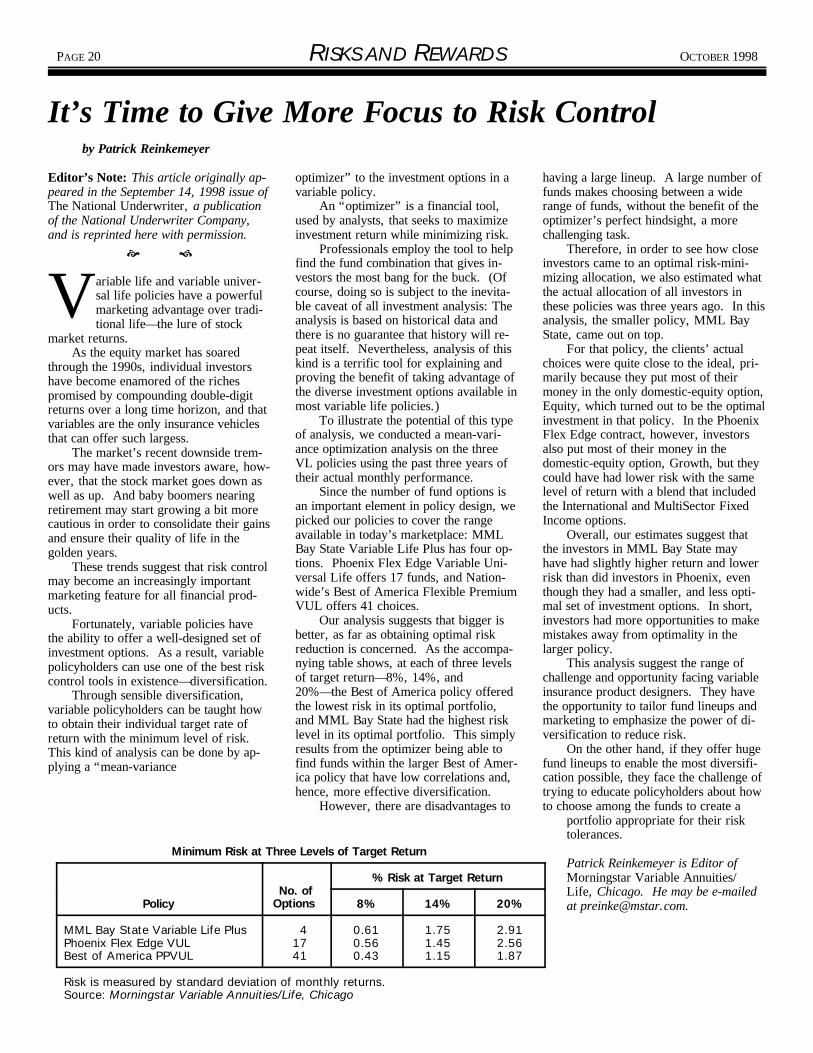
PAGE 20 RISKS AND REWARDS OCTOBER 1998
Minimum Risk at Three Levels of Target Return
No. ofOptions
% Risk at Target Return
Policy 8% 14% 20%
MML Bay State Variable Life PlusPhoenix Flex Edge VULBest of America PPVUL
41741
0.610.560.43
1.751.451.15
2.912.561.87
Risk is measured by standard deviation of monthly returns.Source: Morningstar Variable Annuities/Life, Chicago
It’s Time to Give More Focus to Risk Control by Patrick Reinkemeyer
Editor’s Note: This article originally ap- optimizer” to the investment options in a having a large lineup. A large number ofpeared in the September 14, 1998 issue of variable policy. funds makes choosing between a wideThe National Underwriter, a publication An “optimizer” is a financial tool, range of funds, without the benefit of theof the National Underwriter Company, used by analysts, that seeks to maximize optimizer’s perfect hindsight, a moreand is reprinted here with permission. investment return while minimizing risk. challenging task.
ariable life and variable univer-Vsal life policies have a powerfulmarketing advantage over tradi-tional life—the lure of stock
market returns.As the equity market has soared
through the 1990s, individual investorshave become enamored of the richespromised by compounding double-digitreturns over a long time horizon, and thatvariables are the only insurance vehiclesthat can offer such largess.
The market’s recent downside trem-ors may have made investors aware, how-ever, that the stock market goes down aswell as up. And baby boomers nearingretirement may start growing a bit morecautious in order to consolidate their gainsand ensure their quality of life in thegolden years.
These trends suggest that risk controlmay become an increasingly importantmarketing feature for all financial prod-ucts.
Fortunately, variable policies havethe ability to offer a well-designed set ofinvestment options. As a result, variablepolicyholders can use one of the best riskcontrol tools in existence—diversification.
Through sensible diversification,variable policyholders can be taught howto obtain their individual target rate ofreturn with the minimum level of risk. This kind of analysis can be done by ap-plying a “mean-variance
Professionals employ the tool to help Therefore, in order to see how closefind the fund combination that gives in- investors came to an optimal risk-mini-vestors the most bang for the buck. (Of mizing allocation, we also estimated whatcourse, doing so is subject to the inevita- the actual allocation of all investors inble caveat of all investment analysis: The these policies was three years ago. In thisanalysis is based on historical data and analysis, the smaller policy, MML Baythere is no guarantee that history will re- State, came out on top.peat itself. Nevertheless, analysis of this For that policy, the clients’ actualkind is a terrific tool for explaining and choices were quite close to the ideal, pri-proving the benefit of taking advantage of marily because they put most of theirthe diverse investment options available in money in the only domestic-equity option,most variable life policies.) Equity, which turned out to be the optimal
To illustrate the potential of this type investment in that policy. In the Phoenixof analysis, we conducted a mean-vari- Flex Edge contract, however, investorsance optimization analysis on the three also put most of their money in theVL policies using the past three years of domestic-equity option, Growth, but theytheir actual monthly performance. could have had lower risk with the same
Since the number of fund options is level of return with a blend that includedan important element in policy design, we the International and MultiSector Fixedpicked our policies to cover the range Income options.available in today’s marketplace: MML Overall, our estimates suggest thatBay State Variable Life Plus has four op- the investors in MML Bay State maytions. Phoenix Flex Edge Variable Uni- have had slightly higher return and lowerversal Life offers 17 funds, and Nation- risk than did investors in Phoenix, evenwide’s Best of America Flexible Premium though they had a smaller, and less opti-VUL offers 41 choices. mal set of investment options. In short,
Our analysis suggests that bigger is investors had more opportunities to makebetter, as far as obtaining optimal risk mistakes away from optimality in thereduction is concerned. As the accompa- larger policy.nying table shows, at each of three levels This analysis suggest the range ofof target return—8%, 14%, and challenge and opportunity facing variable20%—the Best of America policy offered insurance product designers. They havethe lowest risk in its optimal portfolio, the opportunity to tailor fund lineups andand MML Bay State had the highest risk marketing to emphasize the power of di-level in its optimal portfolio. This simply versification to reduce risk.results from the optimizer being able to On the other hand, if they offer hugefind funds within the larger Best of Amer- fund lineups to enable the most diversifi-ica policy that have low correlations and, cation possible, they face the challenge ofhence, more effective diversification. trying to educate policyholders about how
However, there are disadvantages to to choose among the funds to create aportfolio appropriate for their risktolerances.
Patrick Reinkemeyer is Editor ofMorningstar Variable Annuities/Life, Chicago. He may be e-mailedat [email protected].

OCTOBER 1998 RISKS AND REWARDS PAGE 21
A 99-Year Prospective Test of an Interest-Rate Theory by Daniel F. Case
Editor’s Note: This article describes a insurance companies published letters of capital) are not accompanied by corre-theory of long-term interest-rate trends from distinguished financiers on the fu- sponding increases in the demand for cap-that was propounded in 1899 by an actu- ture course of the interest rate. Those ital.ary, Charlton T. Lewis. The article then letters were almost unanimous, if I read Lewis also challenged, with respectpresents a preliminary examination of the matter correctly, in predicting further to long-term trends, the theory thathow well that theory stands up in the light decline in the interest rate, as it had been “abundance of money in itself makes in-of 20th-century experience. The purpose declining for some 30 years. The one terest low.”[7] To refute that theory heis to invite more thorough evaluation by man who stood out against that view was offered an example of a marked, sus-any experts who find the theory possibly Mr. Charlton T. Lewis, in his very schol- tained rise in interest rates following dra-useful. arly paper. Anyone interested in this sub- matic discoveries of gold in California
f one wishes to develop, interpret, orIevaluate a 100-year term structure ofinterest rates, one needs a notion ofhow interest rates may behave over
the next 100 years or so. In forming sucha notion one may take a look at the abilityof some theories, including perhaps somemathematical models, to explain interest-rate trends that have occurred in the past.
In addition to seeing how well a the-ory explains the past, it is helpful to seehow well it has predicted the future. Wecannot observe a l00-year future, ofcourse, in the case of theories that werepropounded only recently. In the case ofa theory that was published 100 yearsago, however, we can observe its predic-tive success over a period of 100 years.
This article will discuss a theory thatwas published in 1899. The approach ofthis paper will, accordingly, differ fromthat of a typical research paper. Ratherthan develop a theory on the basis of ob-served facts, this paper will briefly de-scribe the previously developed theoryand then discuss how well it appears tohave stood up since it was published. Fora better understanding of the theory thancan be gained from this paper, readerscan consult the 1899 paper.
The paper in question is “The Nor-mal Rate of Interest” by Charlton T.Lewis, a member of the Actuarial Societyof America [1]. That paper, besides pre-senting a theory, gave both a medium-term and a long-term prediction ofinterest-rate trends. The medium-termprediction was evaluated thus at a 1919meeting of the American Institute of Ac-tuaries:
You will perhaps recall that justabout 20 years ago, one of the large life
ject should certainly read and re-read that and Australia.paper. You know the facts are that Mr. Lewis analyzed interest-rate trends inLewis was right [2]. terms of forces of two types (not sharply
Lewis elaborated on (or clarified) his distinguishable from each other): “wave”theory a bit in a second paper, published forces, “which act within definite andin 1904 [3]. In addition to the two pa- often narrow limits of space or time,” andpers, the discussions of them, and the “tidal” forces, “which act for long peri-above-cited 1919 comments, extensive ods and upon the markets of thecomments on Lewis’ work were made at world.”[8] Among “wave” forces, hea 1920 meeting of the Actuarial Society mentioned government manipulations of[4]. There is a further brief reference the supply and value of money and “sub-dating from 1934 [5]. stitutes for money,” wars and rumors of
Materials and MethodsThe materials for this study are the twoLewis papers cited above (which will bebriefly summarized here) and someinterest-rate and other data from yearsfollowing their publication. The methodwill be first to compare Lewis’ interest-rate predictions with rates and trends sub-sequently experienced. Then a prelimi-nary test of the central assertion of Lewis’theory will be presented.
LEWIS’ THEORY
Lewis’ 1899 paper sets forth his theoryand contains his predictions. The theorypertains to long-terms trends and may besummed up by the following two sen-tences: “On the contrary, all experienceproves that the demand for capital findsits supreme stimulus in the expectation ofproductiveness. This expectation is ex-cited chiefly by discovery and inven-tion.”[6]
In the foregoing excerpt, “On thecontrary” refers to assertions by manyeconomists (six of whom Lewis named)that increased wealth and economic prog-ress of themselves lower interest rates. Lewis found no evidence, in the historicaltrends outlined in his paper, that increasesin wealth (bringing increases in the supply
wars, changes in government spending,seasonal demands for money or credit,and the like.
In order to identify the “tidal”forces, Lewis examined long-terminterest-rate trends during the 19th cen-tury in the light of economic develop-ments. He found that long periods ofrising interest rates were associated withperiods of discovery and invention, whilelong periods of falling interest rates wereassociated with relative stagnation. Hefound such periods, each 20 to 30 yearslong, alternating during the century. Heacknowledged that it might be impossibleto explain completely what caused “thealternations of enterprise and stagnation inthe world of industry and trade,” but,clearly, considered it possible to detectevidence of the beginning of a new cy-cle.[9]
Lewis had in mind a “normal” levelabout which interest rates oscillate underboth wave and tidal forces.
continued on page 22, column 1

PAGE 22 RISKS AND REWARDS OCTOBER 1998
A 99-Year Prospective Testcontinued from page 21
Following a discussion of capital transac- “The reason is that the de- age of interest realized by life insurancetions he wrote, “Since enterprise always mand is determined, not by the companies upon their invested as-stands ready to use capital productively, it experience of past productive- sets.”[16] He observed that a little moreis always willing to exchange for the capi- ness, but by the hope of future than 20 years previously that rate hadtal available at the earlier date a larger profit.”[13] been a full 6% and that it now appearedcapital of a later date, the addition being to have bottomed out at slightly belowlimited only by the expected increase of LEWIS’ PREDICTIONS 5%. He pointed out, in a footnote, thatvalue.”[10] Thus he related the normal the published rates included realized capi-rate of interest to the average rate of pro- tal gains and losses, which caused anductiveness of capital during a time inter- overstatement of the overall yield whenval. interest yields were falling and an under-
Some of Lewis’ discussion of the statement when they were rising. Heaverage rate of productiveness seems also, of course, pointed out that the pub-questionable and was challenged by one lished rates were portfolio, not new-or more discussants of his work. Lewis money, yields. He wrote:did not, however, use that aspect of histheory in arriving at his estimate of thenormal rate of interest. Before turning tothat estimate, however, let us look at twoelaborations, or clarifications, of the the-ory that appear in Lewis’ 1904 paper.
First, Lewis distinguished capitalfrom property. “Property consists of in-dividual things, each of which can be seenand handled, used and enjoyed; each withits own distinct features of utility. … Cap-ital consists of dollars or other ideal unitsof an infinite mass, every one of which isabsolutely identical with everyother.”[11]
Second, Lewis emphasized that theexpectation of productiveness of capital“rests upon the nature of man in a pro-gressive society, and not upon the natureof property. Were the spirit of enterprisedestroyed and the speculative hazards offortune ended, the demand for capital inindustry would be limited to the amountsneeded under old and tried methods ofproduction.”[12] Further:
“Economists have long per-ceived that periods of invention,discovery and enterprise arethose in which the demand forcapital is effective and interesthigh. But the connection be-tween the spirit of enterprise andthe increased demand has alwaysbeen sought in the slow processof absorbing capital in new en-terprises, converting the floatingsupply into fixed forms, and re-ducing the available stock in themarkets. In reality the connec-tion is far closer and the effectupon the rate of interest is muchquicker, than this process canexplain.
Lewis used a two-step procedure in devel-oping the medium-term prediction thatwon praise 20 years later. First, he pro-vided evidence that interest rates werebeginning to head upwards from a pre-sumed low point. He then wrote:
“The forces which have turnedthe great tidal movement areobvious, and are as wide as thecivilized world. Invention andenterprise have taken new lifeeverywhere. … The rapid devel-opment of steam navigation, ofrailway improvement, of shipcanals, of electrical art in a thou-sand forms, the increase ofbuildings, furnaces, mills, ma-chinery, the opening of new col-onies, in short, the conversion offloating into fixed capital, goeson at an accelerating pace. …Whenever hitherto such an epochof invention and enterprise haschecked a long-continued accu-mulation of idle capital andturned the great tidal wave ofinterest from ebb to flow, theprocess has been progressive formany years, and has continued mate of the normal interest rate by histo gain force and rapidity long selected measure. We may regard hisafter it had first become conspic- medium-term prediction as being that; inuous. the absence of war, the rate realized by
… If the world’s peace is life insurers on their invested assetsmaintained, there is not in pros- would rise to at least 5.4%.pect any check to the gradual Lewis acknowledged that further ex-rise of interest, at least until the amination was needed; he regarded hisaverage rate shall fully reflect conclusions as a “working hypothe-the average yield of productive sis.”[18]capital.”[14]
METHOD OF COMPARING PREDICTED WITHLewis then addressed the question ofwhat that average yield—the normal inter-est rate—is. He wrote: “The questionwhat that average yield is demands the tion will be compared with various pub-actuary’s methods applied to the data of lished rates of interest relating to the the economist. My object is to stimulateinquiry, not to dogmatize on its re- continued on page 23, column 1sults.”[15] What follows in Lewis’ paperwas, then, perhaps acknowledged by himto be only an expedient.
Lewis wrote: “There could be nobetter measure of the true normal yield ofinvested capital than the average percent-
“These considerations must betaken into account, and the effectof each estimated in detail toreach the true average rate ofinterest. Such an examinationwould probably prove that thetrue rate in 1897 was consider-ably below the apparent rate of4.92%, and possibly somewhatbelow 4.5%, but that the averagerate for the whole period of de-clining interest from 1872 to1897 was above 5.4%.
“It seems reasonable to be-lieve that this last-named aver-age, taken through a period ofdeclining rates, fairly representsthe permanent average incomefrom safe investments.” [17]We may regard 5.4% as Lewis’ esti-
ACTUAL
Lewis’ medium-term interest-rate predic-

OCTOBER 1998 RISKS AND REWARDS PAGE 23
A 99-Year Prospective Testcontinued from page 22
period 1899–1921. His estimate of the of expectation of productiveness. As in- years, the averages for five-year“permanent average income from safe dicated previously, Lewis asserted that periods are as follows:investments” will be compared with a 99- this expectation is excited chiefly by dis-year average taken from insurers’ portfo- covery and invention. Certainly, thelio yields during the period 1899– 1919 numbers of patents and trademarks issuedand Moody’s Aaa corporate bond yields each year, discussed later in this paper,during the period 1920–97. Lewis’ un- are at best a crude measure of the level ofderlying theory—that the primary “tidal” discovery and invention. The presentforce is the expectation of productive- writer, however, is not knowledgeable inness—will be tested by comparing year- the matters that would have to be ana-by-year new-money yields with the yearly lyzed in order to get a better measure. percent changes in the numbers of U.S. The writer hopes that any experts who arepatents and trademarks issued and in the interested in Lewis’ theory will look forgross domestic product, measured in con- ways to test it more soundly and thor-stant dollars. oughly.
DiscussionA good test of Lewis’ estimate of the“average yield of productive capital”might be a comparison of 5.4% with lifeinsurers’ average new-money investmentyields during the twentieth century. Asan approximation, portfolio yields mightbe used instead. Of course, it might bedifficult or impossible to ascertain pre-cisely how such published numbers werederived at each time during the century. Also, as the mix of investments in insur-ers’ portfolios changed over time, a his-tory of their overall yields might losemeaning as an indicator of interest-ratetrends. The corporate-bond yields usedin this article have the advantages of be-ing new-money rates and being, presum-ably, consistent from year to year.
As for Lewis’ theory, one may ask towhat extent Lewis’ 1899 predictions rep-resent an application of his theory assuch. His paper, presented in October1899, was evidently written that year. Bythat time, according to the paper, new-money interest rates had already started torise, and economic expansion was alreadywell underway. Presumably, the thencurrent period of discovery and inventionhad been going on for some time. Onemight say, therefore, that Lewis’ paper ineffect states that there was evidence that aperiod of discovery and invention hadbegun at some recent time and that histheory predicted that the period wouldcontinue for a good while longer andcarry with it a continuing rise in interestrates. When that period began, how itsbeginning might have been detected, andhow to determine whether it was still inprogress are not stated.
A good test of Lewis’ underlyingtheory would analyze trends in the level
The numbers on gross domesticproduct are included below as a possibleindication of the productiveness that mayhave been expected some years before. Gross domestic rather than gross nationalproduct is used because it focuses on cap-ital located in the U.S., rather than oncapital owned by U.S. interests.
By 1920 it was being suggested thatthere is a strong connection between infla-tion and interest rates. In a discussion ofLewis’ papers in 1920, R.W. Huntingtonremarked, “Mr. Lewis did not have in hismind any clear idea of inflation as a causeof increasing the interest rates.”[19] Lewis’ 1899 paper did mention inflation,as follows: “Each large issue of such cur-rency causes violent fluctuations, first fora very short time in rates of interest ontemporary loans, and then more lastinglyin the nominal prices of goods...”[20] The issuing of currency was classed byLewis as one type of wave force. Ac-cordingly, Lewis treated inflation as aproduct of a wave force. He may or maynot have regarded inflation as itself aforce that acts upon interest rates. In anycase, since he did not include inflation inhis discussion of tidal forces, the follow-ing tests of his predictions and theoryhave not been designed to reflect infla-tion.
ResultsLEWIS’ INTEREST-RATE PREDICTIONS
The following was stated by Douglas H.Rose in the 1920 discussion mentionedabove:
“The Spectator Company is inthe habit of publishing annuallyin its Year Book the rate of inter-est earned on mean investedfunds of a limited number of lifecompanies. Going back 40
1880–1884 5.50% 1885–1889 . . . . . . . . 5.37% 1890–1894 . . . . . . . . 5.15% 1895–1899 . . . . . . . . 4.88% 1900–1904 . . . . . . . . 4.66% 1905–1909 . . . . . . . . 4.77% 1910–1914 . . . . . . . . 4.80% 1915–1919 . . . . . . . . 4.87% [21]Yields on Moody’s Aaa-rated corpo-
rate bonds for the period 1919 (the earli-est year for which such a figure wasfound) through 1997 are shown in TableA.
We can calculate a 99-year averageinterest rate from the data shown aboveand in Table A by using for 1899 theSpectator Company’s number for1895–1899, using the 1900–1919 Specta-tor numbers as if they were new-moneyrates for those years, and using theMoody yields for the years 1920–97. Thejustification for using portfolio rates for1899-1919 is that new-money rates beganthat period somewhat below the portfoliolevel and ended the period somewhatabove it.
The resulting 99-year average is5.65%, a rate slightly above Lewis’ esti-mated normal interest rate of 5.4%. Itmust be noted again, of course, that theMoody yields do not represent the mea-sure that Lewis had in mind. Also, inter-est rates were considerably higher in 1997than in 1895–99. If interest rates do notdecline significantly during the 10 yearsfollowing 1997, an average over the years1909–2007 will be higher than the above5.65% average for 1899–1997.
The Moody’s Aaa yield for 1919, asshown in Table A, is 5.49%, while theinsurers’ portfolio yield for the years1915–19, shown above, is 4.87%. Inorder to guess what the insurers’ new-money yield was in 1919, we may notethat the yield on municipal high-gradebonds rose quite steadily from 3.12% in1900 (the earliest year for which such afigure was found) to
continued on page 24, column 1
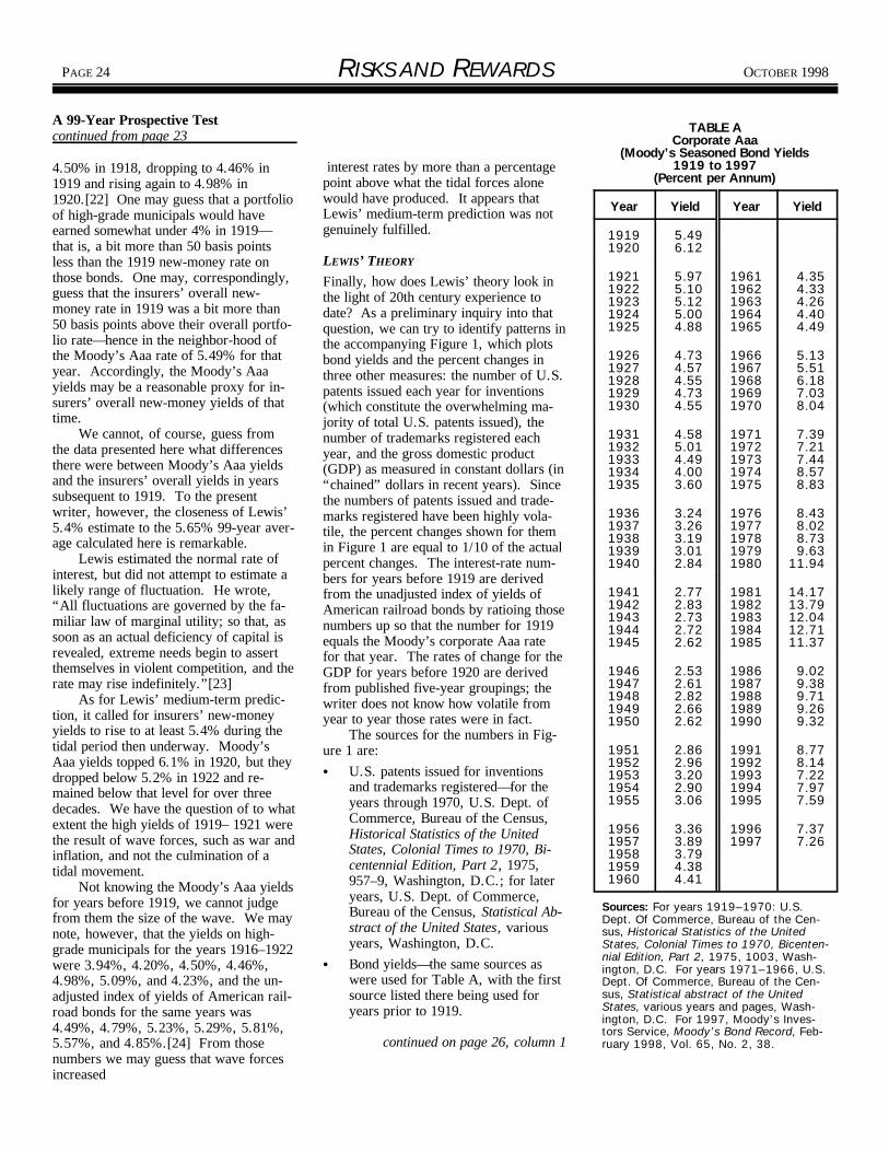
PAGE 24 RISKS AND REWARDS OCTOBER 1998
A 99-Year Prospective Testcontinued from page 23
4.50% in 1918, dropping to 4.46% in1919 and rising again to 4.98% in1920.[22] One may guess that a portfolioof high-grade municipals would haveearned somewhat under 4% in 1919—that is, a bit more than 50 basis pointsless than the 1919 new-money rate onthose bonds. One may, correspondingly,guess that the insurers’ overall new-money rate in 1919 was a bit more than50 basis points above their overall portfo-lio rate—hence in the neighbor-hood ofthe Moody’s Aaa rate of 5.49% for thatyear. Accordingly, the Moody’s Aaayields may be a reasonable proxy for in-surers’ overall new-money yields of thattime.
We cannot, of course, guess fromthe data presented here what differencesthere were between Moody’s Aaa yieldsand the insurers’ overall yields in yearssubsequent to 1919. To the presentwriter, however, the closeness of Lewis’5.4% estimate to the 5.65% 99-year aver-age calculated here is remarkable. Lewis estimated the normal rate ofinterest, but did not attempt to estimate alikely range of fluctuation. He wrote,“All fluctuations are governed by the fa-miliar law of marginal utility; so that, assoon as an actual deficiency of capital isrevealed, extreme needs begin to assertthemselves in violent competition, and therate may rise indefinitely.”[23]
As for Lewis’ medium-term predic-tion, it called for insurers’ new-moneyyields to rise to at least 5.4% during thetidal period then underway. Moody’sAaa yields topped 6.1% in 1920, but theydropped below 5.2% in 1922 and re-mained below that level for over threedecades. We have the question of to whatextent the high yields of 1919– 1921 werethe result of wave forces, such as war andinflation, and not the culmination of atidal movement.
Not knowing the Moody’s Aaa yieldsfor years before 1919, we cannot judgefrom them the size of the wave. We maynote, however, that the yields on high-grade municipals for the years 1916–1922were 3.94%, 4.20%, 4.50%, 4.46%,4.98%, 5.09%, and 4.23%, and the un-adjusted index of yields of American rail-road bonds for the same years was4.49%, 4.79%, 5.23%, 5.29%, 5.81%,5.57%, and 4.85%.[24] From thosenumbers we may guess that wave forcesincreased
interest rates by more than a percentagepoint above what the tidal forces alonewould have produced. It appears thatLewis’ medium-term prediction was notgenuinely fulfilled.
LEWIS’ THEORY
Finally, how does Lewis’ theory look inthe light of 20th century experience todate? As a preliminary inquiry into thatquestion, we can try to identify patterns inthe accompanying Figure 1, which plotsbond yields and the percent changes inthree other measures: the number of U.S.patents issued each year for inventions(which constitute the overwhelming ma-jority of total U.S. patents issued), thenumber of trademarks registered eachyear, and the gross domestic product(GDP) as measured in constant dollars (in“chained” dollars in recent years). Sincethe numbers of patents issued and trade-marks registered have been highly vola-tile, the percent changes shown for themin Figure 1 are equal to 1/10 of the actualpercent changes. The interest-rate num-bers for years before 1919 are derivedfrom the unadjusted index of yields ofAmerican railroad bonds by ratioing thosenumbers up so that the number for 1919equals the Moody’s corporate Aaa ratefor that year. The rates of change for theGDP for years before 1920 are derivedfrom published five-year groupings; thewriter does not know how volatile fromyear to year those rates were in fact.
The sources for the numbers in Fig-ure 1 are:
U.S. patents issued for inventionsand trademarks registered—for theyears through 1970, U.S. Dept. ofCommerce, Bureau of the Census,Historical Statistics of the UnitedStates, Colonial Times to 1970, Bi-centennial Edition, Part 2, 1975,957–9, Washington, D.C.; for lateryears, U.S. Dept. of Commerce,Bureau of the Census, Statistical Ab-stract of the United States, variousyears, Washington, D.C. Bond yields—the same sources aswere used for Table A, with the firstsource listed there being used foryears prior to 1919.
continued on page 26, column 1
TABLE ACorporate Aaa
(Moody’s Seasoned Bond Yields1919 to 1997
(Percent per Annum)
Year Yield Year Yield
1919 5.491920 6.12
1921 5.97 1961 4.351922 5.10 1962 4.331923 5.12 1963 4.261924 5.00 1964 4.401925 4.88 1965 4.49
1926 4.73 1966 5.131927 4.57 1967 5.511928 4.55 1968 6.181929 4.73 1969 7.031930 4.55 1970 8.04
1931 4.58 1971 7.391932 5.01 1972 7.211933 4.49 1973 7.441934 4.00 1974 8.571935 3.60 1975 8.83
1936 3.24 1976 8.431937 3.26 1977 8.021938 3.19 1978 8.731939 3.01 1979 9.631940 2.84 1980 11.94
1941 2.77 1981 14.171942 2.83 1982 13.791943 2.73 1983 12.041944 2.72 1984 12.711945 2.62 1985 11.37
1946 2.53 1986 9.021947 2.61 1987 9.381948 2.82 1988 9.711949 2.66 1989 9.261950 2.62 1990 9.32
1951 2.86 1991 8.771952 2.96 1992 8.141953 3.20 1993 7.221954 2.90 1994 7.971955 3.06 1995 7.59
1956 3.36 1996 7.371957 3.89 1997 7.261958 3.791959 4.381960 4.41
Sources: For years 1919–1970: U.S.Dept. Of Commerce, Bureau of the Cen-sus, Historical Statistics of the UnitedStates, Colonial Times to 1970, Bicenten-nial Edition, Part 2, 1975, 1003, Wash-ington, D.C. For years 1971–1966, U.S.Dept. Of Commerce, Bureau of the Cen-sus, Statistical abstract of the UnitedStates, various years and pages, Wash-ington, D.C. For 1997, Moody’s Inves-tors Service, Moody’s Bond Record, Feb-ruary 1998, Vol. 65, No. 2, 38.

Year90 95 0 5 10 15 20 25
-22-20-18-16-14-12-10-8-6-4-202468
101214161820
.1x Patents .1x TrademarksBond Yield GDP (Real)
Year26 30 35 40 45 50 55 60 65
-22-20-18-16-14-12-10-8-6-4-202468
101214161820
Year66 70 75 80 85 90 95 97
-22-20-18-16-14-12-10-8-6-4-202468
101214161820
OCTOBER 1998 RISKS AND REWARDS PAGE 25
FIGURE 1—Bond Yields vs. Changes in Other Measures
PAGE 26 RISKS AND REWARDS OCTOBER 1998
A 99-Year Prospective Testcontinued from page 24
GDP—for years through 1928, His- registrations). [27] That pattern seems to subsequent experience, to have cometorical Statistics of the United States, offer additional support. quite close to the mark. His medium-Colonial Times to 1970, Bicentennial Real GDP was highly volatile during term prediction regarding a tidal trendEdition, Part 1, 232; for the years most of the 1923–1951 period, and the beginning in about 1898 seems to have1929 through 1958, U.S. Dept. of present writer hazards no speculations been fulfilled with regard to its duration,Commerce, Bureau of Economic about it. but not genuinely with regard to the levelAnalysis, National Income and Prod- An upward interest-rate trend began it would reach.uct Accounts of the United States, in 1951 and lasted until about 1982. Both The present writer hopes that Lewis’Volume 1, 1929-58, 1993, 3, and patent issues for inventions and trademark papers will kindle an interest in furtherVolume 2, 1959–88, 1992, 4, Wash- registrations were on the upswing during investigations along the lines of his the-ington, D.C.; for subsequent years, that period. The patent issues increased ory, with modifications and/or refine-Statistical Abstract of the United from 43,040 in 1950 to 65,800 in 1981. ments as may appear appropriate in theStates, various years. Over the same period, trademark registra- light of 20th century experience and
tions increased from 16,817 to thought.We may first observe the risinginterest-rate trend heralded by Lewis,which lasted through 1920. We see thatin 1899 the levels of patent and trademarkapprovals improved slightly, and if theupsurge of trademark approvals in 1905and 1906 represented in part an effort toreduce a heavy backlog of applications,trademark activity must have been livelyduring the first few years of the century. A similar backlog of trademark applica-tions may have developed during WorldWar I. Overall, patent issues for inven-tions increased from 20,377 in 1898 to43,892 in 1916, and trademark registra-tions increased from 1,238 in 1898 to6,791 over the same period.[25] If patentand trademark approvals are a good indi-cation of the level of discovery and inven-tion and hence of expectations of produc-tiveness, that pattern offers support forLewis’ theory.
On the other hand, real GDP wasincreasing at a lower rate during the last15 years of Lewis’ upward tidal periodthan its rate for many years preceding1905. If that pattern reflects people’sexpectations of productiveness during theperiod of the interest-rate increase, it isevidence against Lewis’ theory.
A downward interest-rate trend beganin about 1922 and continued through1946. We see that patent approvals forinventions were relatively flat from 1921(37,798 issues) through 1941 (41,109issues),[26] decreasing from 1942through 1947, and then increasing fairlyvigorously in 1948–50. Presumably, thewar influenced the pattern from 1942–50. The long, rather flat period through 1941,however, seems to support Lewis’ theory. As for trademark activity, registrationscontinued to increase through 1923(14,834 registrations), were flat fromthen through 1930 (13,246 registrations),and then declined through 1941 (8,530
42,700.[28] Those patterns seem to sup-port Lewis’ theory quite strongly.
There were reasonably healthy in-creases in GDP during most of the1951–1982 period.
A downward interest-rate trend beganin about 1983 and may or may not be stillin progress as of 1998. The trend in pat-ents has been from 65,800 in 1981 to101,700 in 1994, and the trend in trade-marks over the same period has beenfrom 42,700 to 63,900.[29] Those pat-terns offer evidence against Lewis’ the-ory.
Also with respect to real GDP, thetrend from 1981 to 1996 looks not muchdifferent from the trend during the pre-ceding period.
ConclusionsThe present writer has not attempted athorough investigation of whether Lewis’interest-rate theory holds up under 20thcentury conditions. Preliminary findingsseem, however, somewhat encouraging. Interest rates (Moody’s Aaa corporatebond yields ) have continued to followLewis’ observed pattern of “tidal” trends. The lengths of those trends (excluding thedownward trend that began in 1982 or1983 and may or may not still be continu-ing) have been within or close to Lewis’observed 19th century lengths of 20–30years. As for Lewis’ theory that the pri-mary tidal force influencing interest ratesis the expectation of productiveness, theevidence shown in this paper with regardto patent and trademark approvals seemsto support the theory, in varying degrees,with regard to three of the four tidalinterest-rate trends discussed here, butdefinitely not with regard to the trend thatbegan in about 1983.
Lewis’ estimate of the normal rate ofinterest seems, on the basis of 99 years of
End Notes1. Lewis, Charlton T., “The Normal
Rate of Interest,” Actuarial Societyof America Papers and Transactions,1899–1900, Volume VI, Nos. 21,22, 23, and 24, pp. 158–171.
2. American Institute of Actuaries Re-cord, 1919, Volume VIII, pp.309–311.
3. Lewis, Charlton T., “Notes on aFactor, Hitherto Overlooked, of theRate of Interest,” Actuarial Societyof America Transactions, 1904, Vol-ume VIII, Nos. 31, 32, pp. 8–16.
4. “Abstract of Discussion of (‘SomeInfluences Affecting the InterestRate,’ by Wendell M. Strong),” Ac-tuarial Society of America Transac-tions, May 20 and 21, 1920, Vol.XXI, Part One, No. 63, pp.437–451.
5. American Institute of Actuaries Re-cord, 1934, Volume XXIII, p. 134.
6. Lewis, Charlton T., “The NormalRate of Interest,” op. cit., 165.
7. Ibid., 164.8. Ibid., 161.9. Ibid., 166.10. Ibid., 160.11. Lewis, Charlton T., “Notes on a
Factor, Hitherto Overlooked, of theRate of Interest,” op. cit, 9.
continued on page 27, column 1

OCTOBER 1998 RISKS AND REWARDS PAGE 27
A 99-Year Prospective Testcontinued from page 26
12. Ibid., 12. 20. Lewis, Charlton T., “The Normal 24. U.S. Dept. Of Commerce, Bureau ofRate of Interest,” op. cit., 161. the Census, Historical Statistics of13. Ibid., 15–16.
14. Lewis, Charlton T., “The NormalRate of Interest,” op. cit., 168.
15. Ibid., 169.16. Ibid., 169.17. Ibid., 170.18. Ibid., 171.19. “Abstract of Discussion of … (‘Some
Influences Affecting the InterestRate,’ by Wendell M. Strong),” op.cit., 441.
the United States, Colonial Times to21. “Abstract of Discussion of … (‘SomeInfluences Affecting the InterestRate,’ by Wendell M. Strong).” op.cit., 440.
22. U.S. Dept. Of Commerce, Bureau ofthe Census, Historical Statistics ofthe United States, Colonial Times to1970, Bicentennial Edition, Part 2,1975, 1003, Washington, D.C.
23. Lewis, Charlton T., “The NormalRate of Interest,” op. cit., 161.
1970, Bicentennial Edition, Part 2,op. cit., 1003.
25. Sources cited for Figure 1.26. Ibid.27. Ibid.28. Sources cited for Figure 1.29. Ibid.
Daniel F. Case, FSA, is a consulting ac-tuary in Rockville, Maryland.
Review of Financial Journals Reviewed by Edwin A. Martin
Term Structure and InterestRatesThe low Treasury rates and wideningspreads that we’ve experienced latelyhave many of us thinking about the yieldcurve. We reviewed several articles re-lated to interest rates and the yield curve.
“Recovery and Implied Default inBrady Bonds” by Karan Bhanot,Journal of Fixed Income, June1998The author demonstrates that implieddefault probabilities in Brady bondsare significantly higher than a zero-recovery model would suggest. Theanalysis has an impact on the valua-tion of spreads on foreign debt andduration calculations. The numericalexample on Argentine bonds supportsthe author’s conclusion.
“Term Premium Estimates fromZero-Coupon Bonds: New Evi-dence on the Expectations Hy-pothesis” by Upinder S. Dhillonand Dennis J. Lasser, Journal ofFixed Income, June 1998This article is very interesting be-cause of its inconsistency with priorresearch. The authors use zero-cou-pon Treasuries to provide strong evi-dence for liquidity premiums in theterm structure and show that the li-quidity premiums increase with ma-
turity. In additional, they find that Alistair Byrne, and Antti Ilmanen,current forward rates can be used to Financial Analysts Journal,forecast quarterly interest rates. May/June 1998
“Rewards to Extending Maturity”by Dale L. Domian, Terry S.Maness, and William Reichenstein,Journal of Portfolio Management,Spring 1998This article discusses the risks andbenefits of extending the maturity of over the study period.fixed-income investments to increaseyield as well as support for differentterm-structure theories and might beof use to actuaries developing interestrate crediting strategies.
“An Approach to Scenario Hedg-ing” by Charles F. Hill and SimonVaysman, Journal of PortfolioManagement, Winter 1998This article discusses a method ofoptimizing a bond portfolio versusfixed-rate liabilities using only ahandful of scenarios selected usingprincipal components analysis. Fac-tors are developed based on threeyield curve shape changes (shift,twist, and butterfly) and permutationsof those basic shape changes. Theyare used to optimize the portfoliowith better results than durationmatching or key-rate matching.
“What Really Happened to U.S.Bond Yields” by Peter Best,
The authors study the fixed-incomeyields over the last 15 years as wellas several explanatory factors: bondrisk premium, expected inflation, andreal short-term rates. The studyfinds that all three factors have con-tributed to the decline in interest rates
Equity-Indexed AnnuitiesTwo articles on option valuation may beof interest to those involved with equity-indexed annuities. The first is “A Fre-quency Distribution Method for ValuingAveraging Options,” ASTIN Bulletin, No-vember 1997. The author, Edwin H.Neave, finds pay-off frequency distribu-tions to value American and Europeanaveraging options. The author uses adiscrete time, recombining binomial assetprice process. Both geometric and arith-metic averaging options are analyzed.
The second article is “A Closed-Form Approximation for Valuing BasketOptions,” Journal of Derivatives,
continued on page 28, column 1
PAGE 28 RISKS AND REWARDS OCTOBER 1998
Review of Financial Journalscontinued from page 27
Summer 1998. The authors, Moshe Arye Spring 1998 Journal of Portfolio Manage- J.P. Morgan, purveyors of theMilevsky, and Steven E. Posner, demon- ment. Optimal value added is described RiskMetrics®, CreditMetrics® and relatedstrate a technique that approximates the as a function of a manager’s ratio of ac- software products have published refer-sum of the lognormals by an inverted tive return-to-risk as well as an investor’s ence material on its value-at-risk modelsgamma distribution. The results show risk tolerance. The article considers dif- on its web page at www.jpmorgan.com. that the use of the inverted gamma pro- ferent types of fixed-income strategies RiskMetrics® is a portfolio value-at-riskduces very reasonable valuations for and seeks to improve the odds of success model while CreditMetrics® is a credit-Asian and basket options. by taking more of “the right kind of risk based VAR model for bond portfo-
Actuaries interested in learning more risk.” The article discusses how some lios. J.P. Morgan started an on line mag-about low-discrepancy sequences as a market calls, such as interest rate bets, azine, the CreditMetrics® Monitor, whichmethod of reducing the number of simula- are difficult to apply successfully on a can be downloaded fromtions needed to accurately price financial frequent basis. www.jpmorgan.com/instruments might find value in “Low- RiskManagement/CreditMetrics/CreditMDiscrepancy Sequences: Monte Carlo etrics.htm. It includes an article on creditSimulation of Option Prices” by Silvio derivatives, a bank loan recovery study,Galanti and Alan Jung in the Fall 1997 and an article entitled “Uses and AbusesJournal of Derivatives. The authors ex- of Bond Default Rates” by Stephenplain the concept of low-discrepancy se- Kealhofer, Sherry Kwok and Wenlongquences and describe some of the popular Weng, that analyzes the statistical proper-algorithms in the context of valuing stock ties of default rates based on discreteoptions, as well as potential problems bond rating categories (AAA, AA, and sowith the technique. on) and compares them to a continuous
Portfolio ManagementAn interesting view of fixed-income port-folio risk and value-added return is found pages on risk management.in “Bond Managers Need to Take MoreRisk” by Ronald N. Kahn in the
Interesting Web PagesIn this section, we thought we might tryhighlighting a web page oriented towardrisk management. A site that would be ofinterest to actuaries interested in financialrisk management is the ContingencyAnalysis web site atwww.contingencyanalysis.com. The siteis an excellent source for information andpapers on risk analysis and has a helpfulglossary of terms, a list of publications onrisk management and links to other web
scale developed by the authors’ company.
Edwin A. Martin, FSA, is Asset/LiabilityStrategist at Aeltus Investment Manage-ment in Hartford, Connecticut.
Taking Stockcontinued from page 11
financial downturn as in one’s personal the pieces are on the table, and even so, become squeezed, leading to less invest-portfolio. It takes guts to follow the phi- one may only find only a few that fit to- ment and expansion down the road.losophy of investing for the long-term gether. Americans are probably willing towhen prices keep falling. Fundamental- tolerate greater imports as long as theists contend that securities’ prices are be- U.S. economy remains strong. But whencoming “quite attractive” while market the U.S. economy slows, we could betechnicians warn that stock markets (de- hearing calls for import “restrictions” andspite short-term blips) are headed much protection for U.S. workers from foreignlower, and the bear market will last until competition and trade, as we may recallat least the middle of 1999. Either way, occurred in the late 1980s. If history re-we must remember that the art of invest- peats itself, then we will all be in for aing is as much psychological as it is a very rough ride. And we may find thatfinancial decision. And there is no free capitalism, which has been fought for bylunch. Western powers so vehemently since
It takes pain to do the research, there World War II, will not be the economicwill always be mistakes, and it involves strategy of choice for many importantpatience. But there is also is no guaran- countries of the world because they havetee that certain results will always be now tried it and, for them, it does notachieved, even over the long-term. That work.is why many are stimulated by working inthe investment industry or studying the Nino Boezio, FSA, is a Principal atfinancial markets. It is a puzzle that has Matheis Associates Benefits Consultants,too many pieces, one never knows if all Inc., in Pickering, Ontario.
The End Of Globalization?It is peculiar that the 1920s was character-ized by inflating stock markets, deflation,and globalization. When financial mar-kets collapsed, globalization was replacedby protectionism and nationalism. Defla-tion was already being seen in our eco-nomic cycle in 1996 (a year before theAsian crisis) as commodity prices starteda downtrend. And despite strong U.S.growth, inflation measures continued toremain low, which bewildered officials atthe Federal Reserve. Perhaps like the1920s, we were already in a situation be-fore the problems surfaced in Asia, wheregains from production were outstrippingincreases in demand. When deflationoccurs, corporate earnings and profits

OCTOBER 1998 RISKS AND REWARDS PAGE 29
“When it was finally acknowledged that the funda-mentals of the Canadian economy had to bechanged and that currency free-fall was just asymptom, there were some offers to the Canadianpublic of all-round tax cuts to stimulate consumerdemand.”
What One Can Learn from the Bank of Canada by Nino Boezio
anada, like many countries, was funds rate was at 5.5% p.a.. This rate Rates Strengthen A Currency?” in theCconsidered to be a dramatically was lower because the Canadian economy Sept. 1994 issue of Risks and Rewards)rising star in early 1997. Even was still perceived to be in a much and that any attempt to prop up the dollarthough it, like most of the West- weaker state of growth than its U.S. by the Bank would be met by renewed
ern world, was a debt-laden country, it counterpart, and hence required more selling and even lower currency values,took major steps to cut spending and monetary stimulus. unless economic prospects were im-bring its fiscal house in order. And as When the Asian crisis took center proved. Also, the wisdom behind Bankwith most, falling interest rates helped stage in the fall of 1997, the Canadian intervention was increasingly coming un-alleviate its debt problem as less of its dollar began to sag and approached the der attack as outdated and inappropriatefiscal budget was required for debt fi- psychologically important level of 70¢ and thus the Bank was losing credibilitynancing. Canada, like Europe, was being U.S. Even though all other commodity- very quickly.seen as a late bloomer from the severe based currencies were suffering much It was also difficult for the Bank torecession of the early 1990s and, hence, it more (the Australian currency that was change its image. It would claim that ithad a lot of fast catching up to do to the initially higher in value to the U.S. dollar no longer cared or would let the currencyUnited States and the United Kingdom. than $Can but was now already trading in float more freely, but everyone knew thatEven though taxes were still high, this the 65¢ range) the Bank of Canada re- the Bank would try to strike periodicwas not seen as a major impediment in a fused to accept this worldwide phenomena blows to short-sellers. It was also ratherworld where Canadian industry and ex- and “drew a line inports would soon be in full gear. High the sand.”unemployment and weak consumer de- It first ap-mand in preceding years meant that wage proached the problempressures and inflation would not materi- by selling its foreignalize for a very long time. This combina- currency reserves totion of fundamentals overall suggested buy Canadian dollarsthat Canada would have economic growth which only providedpossibly higher than any of the other G-7 temporary relief. nations in the coming years. It was also Then by ill-advisedincreasingly being suggested that the Ca- advice from variousnadian dollar ($Can) could eventually rise economists who claimed that short-term confusing when the Canadian Prime Min-above 80¢ U.S. by 1998 or 1999. money rates were too low relative to that ister would claim that the falling dollar
The Asian crisis helped to change all of the U.S. and should be increased, the was good for the economy in that it wouldthat, as it has for most of the world. Bank raised its call money rate to 5%. It stimulate exports and thus no furtherEven though still in trade surplus, the is difficult to say whether this rate rise Bank intervention was necessary, only toCanadian surplus fell greatly because of slowed the Canadian economy down sig- find the Bank intervening a few daysfalling commodity demand. The funda- nificantly, but it can be noted that major later.mentals for Canadian companies no lon- gains in economic growth and declines in When it was finally acknowledgedger looked as good, particularly when unemployment halted soon after. This is that the fundamentals of the Canadianapproximately 40% of Canadian exports also somewhat puzzling considering that economy had to be changed and that cur-are commodity-related. the Canadian and U.S. economies have rency free-fall was just a symptom, there
Because fundamentals were no longer historically been closely-linked and tend were some offers to the Canadian publicas attractive (as can also be said for the to prosper and suffer together at a similar of all-round tax cuts to stimulate con-Asian and South American economies, magnitude. sumer demand. High taxes were an issueAustralia and Eastern Europe) less for- The currency eventually broke below of contention for years but it was sus-eign investment took place, leading to a 70¢ U.S. and the Bank was reluctant to pected that the Federal government wasfalling currency. And even though the raise rates further without endangering the partially unwilling to cut taxes (evenfalling currency was mainly tied to weak- economy. It spent billions of dollars in though it could afford to do so) because itening fundamentals (and strong funda- foreign reserves and used borrowing and wanted to give such “goodies” away in amentals underlying the U.S. dollar driv- the selling of securities to buy $Can, to future election year. As ing up that currency) the Bank of Canada little ultimate avail. Each successive in-tried to fix the problem through monetary tervention was also increasingly unsuc- continued on page 30, column 1mechanisms. cessful and currency speculators became
Short-term interest rates in Canada no longer afraid of the Bank. Currencywere much lower than that of the United traders began to realize that economicStates in early 1997. Call money was at fundamentals “rule” (one can read my3% p.a. whereas the equivalent U.S. Fed article “Does Raising Domestic Interest

PAGE 30 RISKS AND REWARDS OCTOBER 1998
Bank of Canadacontinued from page 29
a result, the government lost the initiative sponded to currency declines by interven- who had put up a discount rate to defendand was finding itself becoming reactive tion or interest rates, is learning that these a gold-exchange parity?) Yet such poli-rather than proactive to the currency cri- are only short-term solutions and are cies are the very ones being widely imple-sis. Unfortunately, economic confidence probably much more short-term than was mented today.”had been so badly shaken that such an the case in the past. The currency mar- A currency is only as strong as itsapproach would not likely produce too kets today are much larger and therefore economy even though there may bemuch in the way of positive results in the market forces will reward and punish its swings in the short term. If investorsnear-term. The tax-cut announcement players more swiftly. A financial body want to go there, businesses want to in-was met with a further decline in the cannot force a certain price or currency vest and sell there, people are buying$Can, which was a combination of scepti- level to be accepted without adverse con- there, and the tax and politic climate iscism, too-little-too-late, or just worries sequences elsewhere. Unfortunately, accommodating, then a strong currencyabout the prospects for further debt re- these should have been lessons learned will follow. That is why everyone at theduction if the tax cuts were made. It from bygone eras. As pointed out in time of this writing wants $US. Onlywould not be a quick fix. It also still has Grant’s Interest Rate Observer (August when the mood changes can the currencyto be realized that Canadian fundamen- 14, 1998, pg. 3) “raising interest rates experience a major shift in value againsttals, like those of most countries today, and tightening monetary growth in the other currencies. The only sign ofare largely affected by what is occurring face of an economic downturn are the strength in $Can (after it fell to 63 cents)in the global village and any attempt to very policies that the modern age was was apparently when commodity pricesdivorce an economy from such impacts is presumed to have outgrown (How many stabilized or moved up.difficult, if not impossible. of today’s policy makers read the history
SummaryHopefully the Bank of Canada, and anyother foreign central banks that have re-
of the Great Depression in graduate Nino Boezio, FSA, is a Principal atschool and shook their heads at the sheer Matheis Associates Benefits Consultants,blockheadedness of the central bankers Inc., in Pickering, Ontario.

OCTOBER 1998 RISKS AND REWARDS PAGE 31
“With the mushrooming of several financialmathematics programs at major universities,firms can now hire a person who requires sub-stantially less in-house ‘conversion.’ The pro-gram purports to train students to be “financialengineers’.”
Competing Education by Zain Mohey-Deen
o perform the complex quantita- have the distinct advantage of being able Technological initiatives being developedTtive analysis in pricing derivative to combine study of the theory with on- by the SOA will address some of theseproducts, investment and com- the-job practice if they work in the invest- concerns. For example, by posting ques-mercial banks have hired from the ment department of an insurance company tions on the web site, access to a larger
ranks of mathematicians, physicists and or are involved in asset/liability manage- group of students and practitioners is pos-actuaries—persons also deemed to be in- ment, pricing, or cash-flow testing for sible. The redesign of the examinationclined towards the investment field. The investment-oriented insurance products. system will also help bridge the gap—thecommercial and investment banks ascer- Even financial math programs with well- new Course Seven is an on-site intensivetained that these individuals had the nec- developed internship arrangements will seminar in modeling. There is a strongessary mathematical skill, and these banks not be able to match this traditional body of academic and practitioner actuar-later supplemented that ability with in- strength. Moreover, through job rota- ies that stand ready to provide this train-house training to “convert” these profes- tions, the actuary’s overall knowledge of ing. Some of the academic actuaries aresionals to the investment industry. With his financial institution is much broader— already on the faculty in financial maththe mushrooming of several financial actuaries know how the other areas in the programs.
mathematics programs at major universi- grams is the cost. In some cases tuition use of these courses to supplement tradi-ties, firms can now hire a person who for the program can be as high as tional continuing education. It may alsorequires substantially less in-house “con- $30,000. make sense to forge alliances with theseversion.” The programs purport to train On the other hand, the financial math institutions, particularly where there arestudents to be “financial engineers.” courses have a more interactive approach actuaries on faculty, to enhance our regu-Conversely, graduates of these programs in learning. The training is laboratory lar education effort. Some programs arehave skills which are attractive to the tra- intensive. Sophisticated software is offered by the mathematics department,ditional employers of actuaries. We licenced to these programs. In general, others within the business school or, inshould be aware of them as our potential students are less isolated and have a better some cases, the engineering school. Fi-competitors, primarily in our emerging opportunity to ask and resolve questions nancial Math programs are offered in thepractice areas, but eventually on our tra- by discussing with other students and fac- major cities in Canada and the U.S. Forditional turf. To start with, we should ulty. The nature of the field is such that those interested in investigating further, ahave a degree of familiarity with the aca- it is easier to develop an understanding of sample of the universities offering suchdemic programs in which they train. the material by “playing” with models. courses and their web sites is provided
There is substantial overlap between To some extent, these advantages can be below:the SOA Investment track syllabus and overcome by the use of technology. the curriculum for these courses. Stu-dents taking SOA courses
organization operate and The travel time involved in the SOAfit together. Beyond the examination system is another disadvan-mathematics of pricing, tage. On a full-time basis, a Master’s inthe actuary knows market- financial math can be obtained in nineing, underwriting, finan- months, and a part-timer could completecial reporting, administra- the course in anywhere from nine monthstion, and so on. The actu- to three years. Once again, the SOAary is a better rounded exam redesign may help overcome thisfinancial professional—at disadvantage.least as to insurance com- It is worthwhile for actuaries to havepanies. Another disadvan- some familiarity with these programs. Intage of these school pro- some cases actuaries may be able to make
Carnegie Mellon University fastweb.gsia.cmu.edu/MSCFColumbia University www.math.columbia.edu/department/masters_finance.shtmlCornell University www.orie.cornell.edu/meng/brochure/tables/financial1.htmlMIT web.mit.edu/sloan/wwwNew York University www.math.nyu.edu/programs/math_fin.htmlOregon Graduate Institute www.cse.ogi.edu/CompFin/University of Chicago finmath.uchicago.eduUniversity of Toronto www.math.toronto.edu/finance
Zain Mohey-Deen, FSA, is a Research Actuary on the Society of Actuaries’ staff in Schaumburg, Illinois.

PAGE 32 RISKS AND REWARDS OCTOBER 1998
Fair Value Conference by Shirley Hwei-Chung Shao
he Society of Actuaries and New (for example, earning emergence pat-TYork University join forces again! tern): These uses/needs can come fromA conference on “Fair Value of statutory regulators (for example, theInsurance Business” will be held Valuation Task Force work, dynamic sol-
on March 18 and 19, 1999 in New York vency analysis), GAAP, InternationalCity. Please mark your calendar and in- Accounting Standards Committee (IASC),form your colleagues in the financial the investment community (for example,management community of this event of rating agencies, analysts), and companythe year! We are also looking for papers management (asset liability management,to enrich this conference. risk management, performance measure-
The goal of the conference is to ex- ments, hedging strategies). Can the vari-tend and update the body of knowledge ous uses/needs be met using a single “fairfrom the first conference two years ago, value” framework?to highlight similarities in various theoret-ical developments, and to work towardsresolution of differences and implementa-tion issues. The scope of the conferencehas been broadened to address fair valua-tion efforts which consider insurancebusiness as an integrated whole.
This conference will:Provide an overview and comparisonof various theoretical developments liability side (which is intuitively uncom-
fortable).Provide an update on various effortsin accounting and management re-porting common ground on the following issues?Suggest how the various theories maybe applied to financial reporting and flows: What’s “free” and for whosemanagement uses in practice purpose is it “free”?Discuss implementation issues andpotential solutions. for mutual companies: Are they in-
deed “free” cash flows?A call for papers is being held inconjunction with the conference. The We hope for your participation in thisgoal of this call for papers is to promote conference, either as a paper presenter orfresh perspectives on this challenging an attendee, because we believe this to betopic, to provide a solid foundation for a very important issue for our professionthe conference, and to advance the state ple think of using this process only for to address. So, look up more informationof the art on insurance valuation. Papers interest rate sensitivity, it can be applied on papers on the web site and watch forshould discuss fair value accounting for to other risk drivers, for example, mortal- registration information in January. Weinsurance with respect to recent develop- ity. promise this conference to be thoughtments in accounting initiatives as well as provoking!management practices.
We would particularly would like to Shirley Hwei-Chung Shao, FSA, is Vicereceive papers on: President and Associate Actuary at theSummaries of the various uses and the Prudential Insurance Company in New-common and unique needs for each user ark, New Jersey, and Chairperson of the
Discount Rates. It seems that most theo-retical developments are variations of discounted cash-flow approaches. Inthese cases, what should be used as thediscount rate/curve (that is, what shouldbe the risk spread over then current Trea-suries)? It is particularly confusing on theliability side when the risk premiumswork in the opposite direction from the
Cash-Flow Components. Can we find
Free cash flows versus all cash
How to treat policyholder dividends
What to do when liabilities depend onasset performance (e.g., creditinginterest rate strategy, dividends)?
Stochastic Process. Although most peo-
How to develop a credible process(because it probably cannot be vali-dated in the market)? For example,how to derive the option value?
How to improve the speed of calcula-tion (for example, low frequencydistribution technology)?
Confidence Level. Should there be anymargins (or just expected value) built inthe fair values? The NAIC project refersto this at various points on the S curve(survivorship function). It attempts tofulfill multiple needs/uses under a singleframework by selecting different pointson the S curve. Liability Floor. Is it necessary to havecash values as the floor since we alreadyhave that in the statutory valuations? ForGAAP, some would say there is no suchfloor with the establishment of deferredacquisition costs. The cash-value floordoes not exist for most company manage-ment uses. Liability Selection. At the last confer-ence, FASB seemed to be interested inknowing whether all liabilities should be“fair valued” since it selected only certainassets (for example, available for publicsale) to be fair valued.
The call for papers also encouragesdiscussions beyond insurance liabilities,including interaction with assets and/orinsurance enterprise value. More infor-mation on the call for papers can be foundon the SOA web site aswww.soa.org\research\cfp2.html.
Financial Reporting Section Council.