r course overheads
TRANSCRIPT
8/6/2019 R Course Overheads
http://slidepdf.com/reader/full/r-course-overheads 1/49
A List of Topics
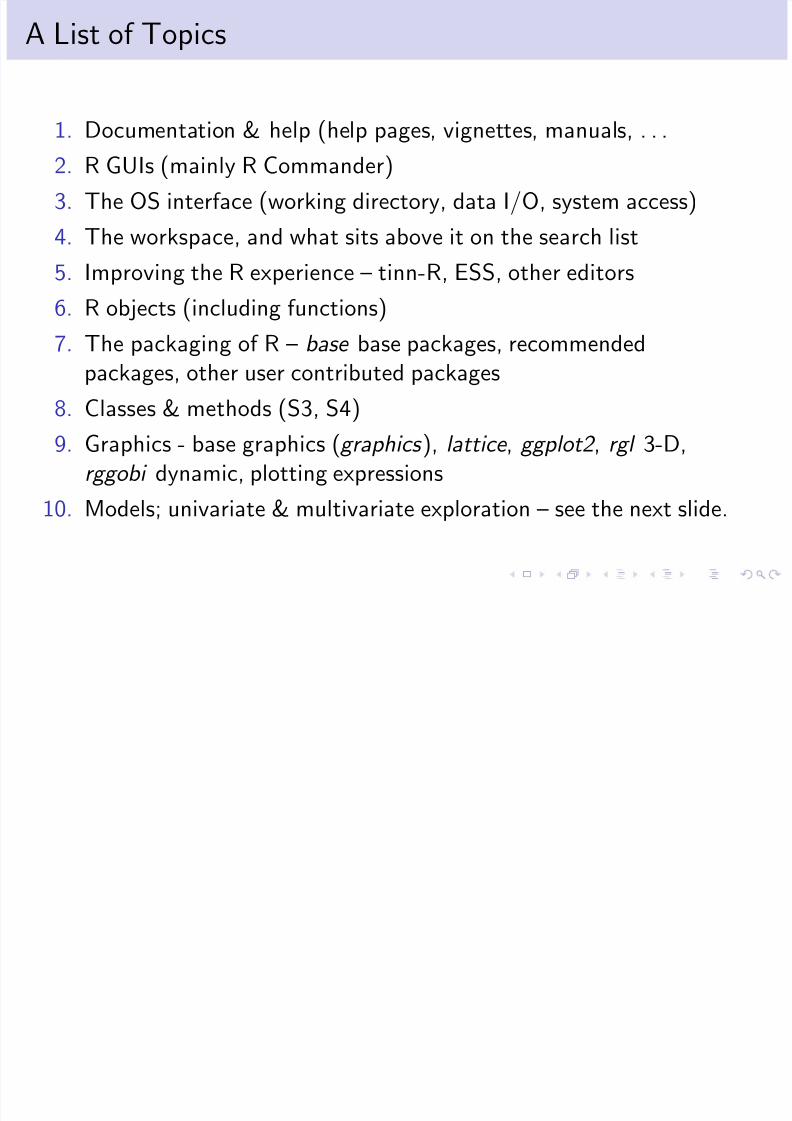
1. Documentation & help (help pages, vignettes, manuals, . . .2. R GUIs (mainly R Commander)
3. The OS interface (working directory, data I/O, system access)
4. The workspace, and what sits above it on the search list
5. Improving the R experience – tinn-R, ESS, other editors6. R objects (including functions)
7. The packaging of R – base base packages, recommendedpackages, other user contributed packages
8. Classes & methods (S3, S4)9. Graphics - base graphics (graphics ), lattice , ggplot2 , rgl 3-D,
rggobi dynamic, plotting expressions
10. Models; univariate & multivariate exploration – see the next slide.

8/6/2019 R Course Overheads
http://slidepdf.com/reader/full/r-course-overheads 2/49
Topics that may be discussed upon request
Package construction
Environments, manipulating language constructs, . . . Models
linear (NB, linear in the parameters) GLM multi-level time series classification
Multivariate exploration distance measures ordination

8/6/2019 R Course Overheads
http://slidepdf.com/reader/full/r-course-overheads 3/49
The R System:
R is currently the environment of choice for specialists who are implementing new methodology highly trained professional data analysts. increasingly, statistically skilled scientists.
It is designed for interactive use: the next step may depend onthe previous result.
Twice-yearly major releases bring improvements & new features. It can be remarkably efficient, even though:
data resides (mostly) in memory it is an interpreted language (but one command may start a
lengthy computation)
8/6/2019 R Course Overheads
http://slidepdf.com/reader/full/r-course-overheads 4/49
Web Sites
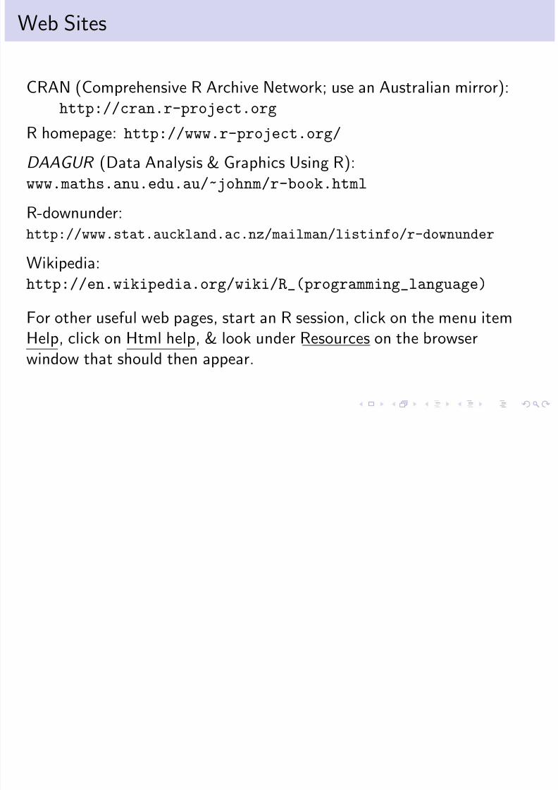
CRAN (Comprehensive R Archive Network; use an Australian mirror):http://cran.r-project.org
R homepage: http://www.r-project.org/
DAAGUR (Data Analysis & Graphics Using R):www.maths.anu.edu.au/
~johnm/r-book.html
R-downunder:http://www.stat.auckland.ac.nz/mailman/listinfo/r-downunder
Wikipedia:
http://en.wikipedia.org/wiki/R_(programming_language)
For other useful web pages, start an R session, click on the menu itemHelp, click on Html help, & look under Resources on the browserwindow that should then appear.
8/6/2019 R Course Overheads
http://slidepdf.com/reader/full/r-course-overheads 5/49
Packages (ss 1.2.2 & Secx 4.21 )
Under Windows & the MacOS X, with an internet connection,use the relevant R menu item to install packages.(usually easier than downloading, then installing).
Note the CRAN task views, which may help in locating packages.
Packages do most of R’s work. They make the system extendablewithout limit.
1Ch, Sec and ss refer to the 3rd edition of Data Analysis and Graphics Using R .
Chx, Secx and ssx refer to the Additional Notes that are available from mywebpage.
8/6/2019 R Course Overheads
http://slidepdf.com/reader/full/r-course-overheads 6/49
Command line calculations (ss 1.1.1)
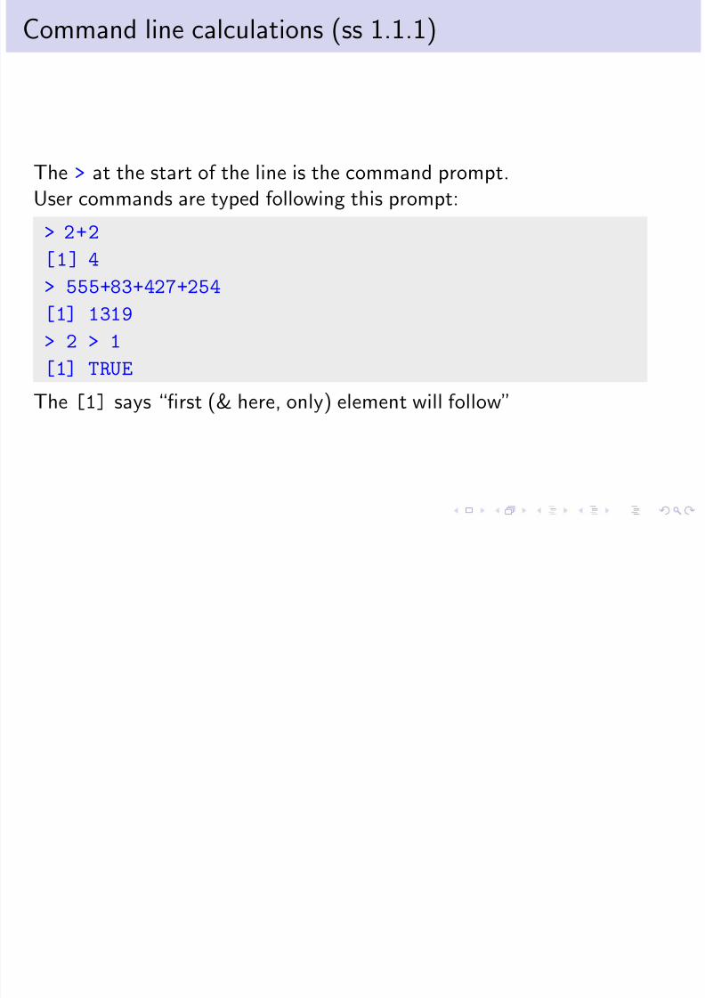
The > at the start of the line is the command prompt.User commands are typed following this prompt:
> 2+2
[1] 4
> 555+83+427+254
[1] 1319
> 2 > 1
[1] TRUE
The [1] says “first (& here, only) element will follow”

8/6/2019 R Course Overheads
http://slidepdf.com/reader/full/r-course-overheads 7/49
Syntax (ss 1.1.1)
Command End of line (providing command is complete) or ;
separator print(2+2); print(2+3)
Quitting To quit from R typeq() # NB q(), not q
Case matters volume is different from Volume
Assignment The assignment symbol is <-, e.g.volume <- c(351, 955, 662, 1203, 557)
# Store the column of numbers in volume
Comments Introduce with #
8/6/2019 R Course Overheads
http://slidepdf.com/reader/full/r-course-overheads 8/49
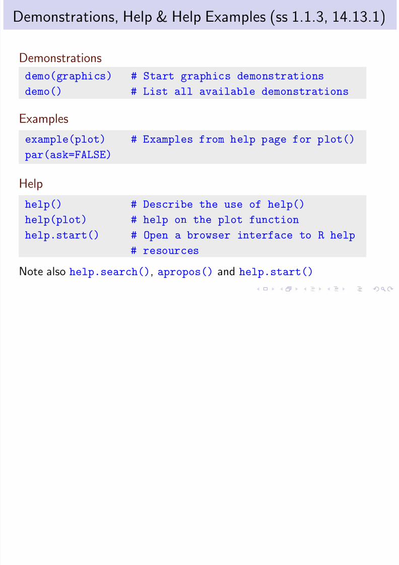
Demonstrations, Help & Help Examples (ss 1.1.3, 14.13.1)
Demonstrations
demo(graphics) # Start graphics demonstrations
demo() # List all available demonstrations
Examples
example(plot) # Examples from help page for plot()par(ask=FALSE)
Help
help() # Describe the use of help()help(plot) # help on the plot function
help.start() # Open a browser interface to R help
# resources
Note also help.search(), apropos() and help.start()

8/6/2019 R Course Overheads
http://slidepdf.com/reader/full/r-course-overheads 9/49
Utility Functions (ss 1.5.1)
Functions that act on the contents of the workspacels() # List contents of workspace
ls(pattern="cr") # List objects whose names include the
# character string "cr"
rm(x, y, z) # Remove x, y, and z from workspacerm(list=c("x", "y", "z")) # Alternative to rm(x, y, z)
rm(list=ls()) # Remove contents of workspace
Functions that access the working or other specified directory
## Functions that act on the working or other directory
dir() # List contents of working directory
file.show() # List file contents on screen.
8/6/2019 R Course Overheads
http://slidepdf.com/reader/full/r-course-overheads 10/49
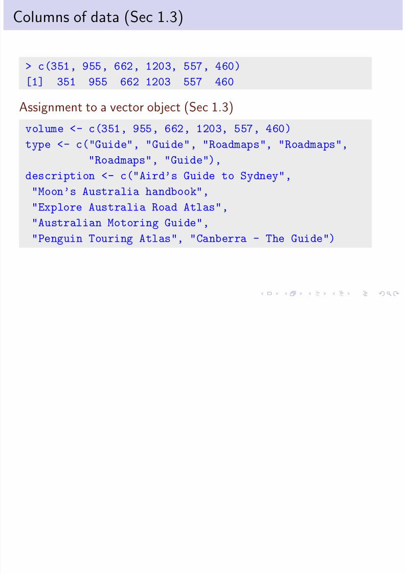
Columns of data (Sec 1.3)
> c(351, 955, 662, 1203, 557, 460)[1] 351 955 662 1203 557 460
Assignment to a vector object (Sec 1.3)
volume <- c(351, 955, 662, 1203, 557, 460)
type <- c("Guide", "Guide", "Roadmaps", "Roadmaps","Roadmaps", "Guide"),
description <- c("Aird’s Guide to Sydney",
"Moon’s Australia handbook",
"Explore Australia Road Atlas","Australian Motoring Guide",
"Penguin Touring Atlas", "Canberra - The Guide")

8/6/2019 R Course Overheads
http://slidepdf.com/reader/full/r-course-overheads 11/49
Data Frames – Lists of Columns (Sec 1.4)
thickness <- c(1.3, 3.9, 1.2, 2, 0.6, 1.5)
width <- c(11.3, 13.1, 20, 21.1, 25.8, 13.1)
height <- c(23.9, 18.7, 27.6, 28.5, 36, 23.4)
weight <- c(250, 840, 550, 1360, 640, 420)
## volume, type & description were input earlier?
This can get unmanageable (many objects). We might prefer:
travelbooks <- data.frame(
thickness = c(1.3, 3.9, 1.2, 2, 0.6, 1.5),
width = c(11.3, 13.1, 20, 21.1, 25.8, 13.1),
. . . .type = type # type was created earlier
row.names = description # description was created earli
)
Data frames offer a tidy way to supply data to modeling functions.
8/6/2019 R Course Overheads
http://slidepdf.com/reader/full/r-course-overheads 12/49
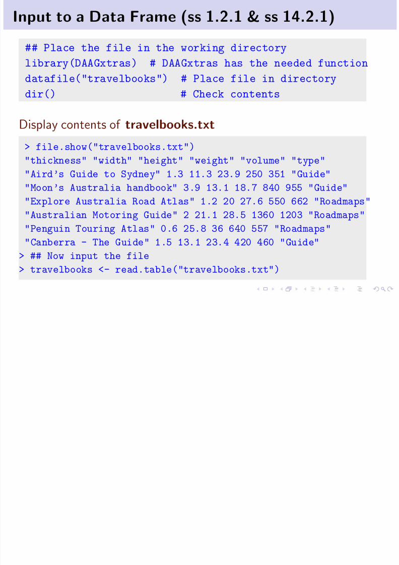
Input to a Data Frame (ss 1.2.1 & ss 14.2.1)
## Place the file in the working directory
library(DAAGxtras) # DAAGxtras has the needed function
datafile("travelbooks") # Place file in directory
dir() # Check contents
Display contents of travelbooks.txt
> file.show("travelbooks.txt")
"thickness" "width" "height" "weight" "volume" "type"
"Aird’s Guide to Sydney" 1.3 11.3 23.9 250 351 "Guide"
"Moon’s Australia handbook" 3.9 13.1 18.7 840 955 "Guide"
"Explore Australia Road Atlas" 1.2 20 27.6 550 662 "Roadmaps"
"Australian Motoring Guide" 2 21.1 28.5 1360 1203 "Roadmaps"
"Penguin Touring Atlas" 0.6 25.8 36 640 557 "Roadmaps"
"Canberra - The Guide" 1.5 13.1 23.4 420 460 "Guide"
> ## Now input the file
> travelbooks <- read.table("travelbooks.txt")
8/6/2019 R Course Overheads
http://slidepdf.com/reader/full/r-course-overheads 13/49
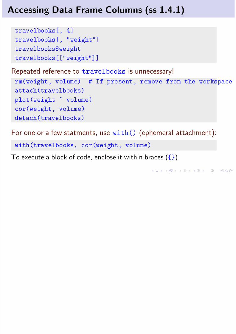
Accessing Data Frame Columns (ss 1.4.1)
travelbooks[, 4]
travelbooks[, "weight"]travelbooks$weight
travelbooks[["weight"]]
Repeated reference to travelbooks is unnecessary!
rm(weight, volume) # If present, remove from the workspaceattach(travelbooks)
plot(weight ~ volume)
cor(weight, volume)
detach(travelbooks)
For one or a few statments, use with() (ephemeral attachment):
with(travelbooks, cor(weight, volume)
To execute a block of code, enclose it within braces ({})

8/6/2019 R Course Overheads
http://slidepdf.com/reader/full/r-course-overheads 14/49
The Working Environment (ss 1.1.1, Sec 1.8 & ss 14.1.2
Working R will by default read files from this directory,
directory or write files to itObject A data structure or function that R recognizes
Functions, as well as data, exist as “objects”Note also, e.g., formula objects, expression objects, . . .
Workspace This is the user’s “database”, where the user can makeadditions or changes, or delete objects, as desired.Use ls() to list contents of current workspace.
read.table() Use to read data, from a file, into the workspace
Image files Use to store R objects, e.g., workspace contents.(The expected file extension is .RData or .rda)
save.image() Use to store all or some workspace contents.For safety, use from time to time in a session
Alternatively, use the relevant menu item.
8/6/2019 R Course Overheads
http://slidepdf.com/reader/full/r-course-overheads 15/49
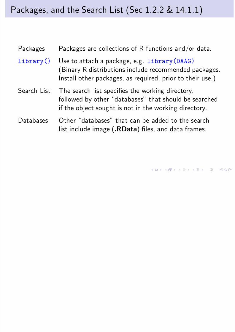
Packages, and the Search List (Sec 1.2.2 & 14.1.1)
Packages Packages are collections of R functions and/or data.
library() Use to attach a package, e.g. library(DAAG)
(Binary R distributions include recommended packages.Install other packages, as required, prior to their use.)
Search List The search list specifies the working directory,followed by other “databases” that should be searchedif the object sought is not in the working directory.
Databases Other “databases” that can be added to the searchlist include image (.RData) files, and data frames.
( )
8/6/2019 R Course Overheads
http://slidepdf.com/reader/full/r-course-overheads 16/49
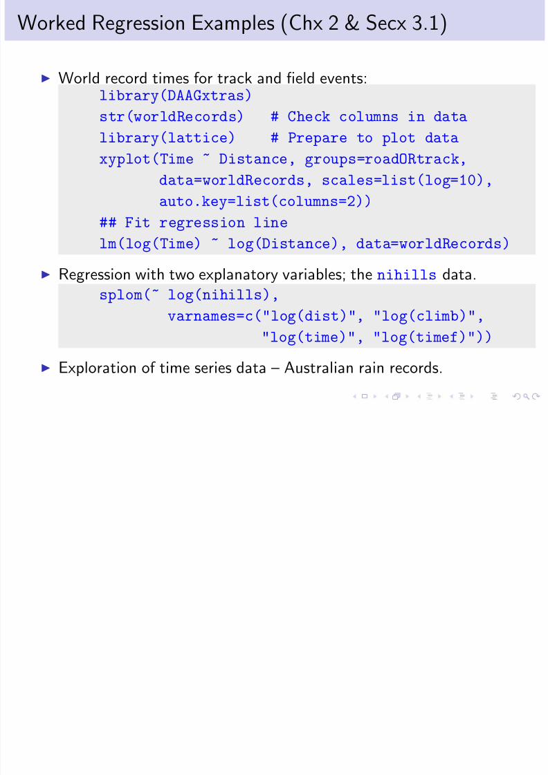
Worked Regression Examples (Chx 2 & Secx 3.1)
World record times for track and field events:
library(DAAGxtras)str(worldRecords) # Check columns in data
library(lattice) # Prepare to plot data
xyplot(Time ~ Distance, groups=roadORtrack,
data=worldRecords, scales=list(log=10),
auto.key=list(columns=2))
## Fit regression line
lm(log(Time) ~ log(Distance), data=worldRecords)
Regression with two explanatory variables; the nihills data.splom(~ log(nihills),
varnames=c("log(dist)", "log(climb)",
"log(time)", "log(timef)"))
Exploration of time series data – Australian rain records.
Diff f d bj
8/6/2019 R Course Overheads
http://slidepdf.com/reader/full/r-course-overheads 17/49
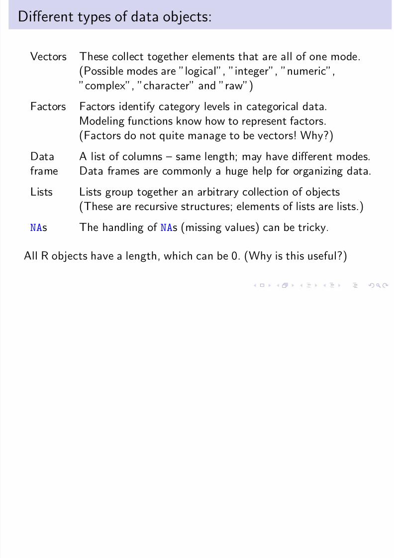
Different types of data objects:
Vectors These collect together elements that are all of one mode.
(Possible modes are ”logical”, ”integer”, ”numeric”,”complex”, ”character” and ”raw”)
Factors Factors identify category levels in categorical data.Modeling functions know how to represent factors.
(Factors do not quite manage to be vectors! Why?)Data A list of columns – same length; may have different modes.frame Data frames are commonly a huge help for organizing data.
Lists Lists group together an arbitrary collection of objects
(These are recursive structures; elements of lists are lists.)
NAs The handling of NAs (missing values) can be tricky.
All R objects have a length, which can be 0. (Why is this useful?)
V (S 1 3)
8/6/2019 R Course Overheads
http://slidepdf.com/reader/full/r-course-overheads 18/49
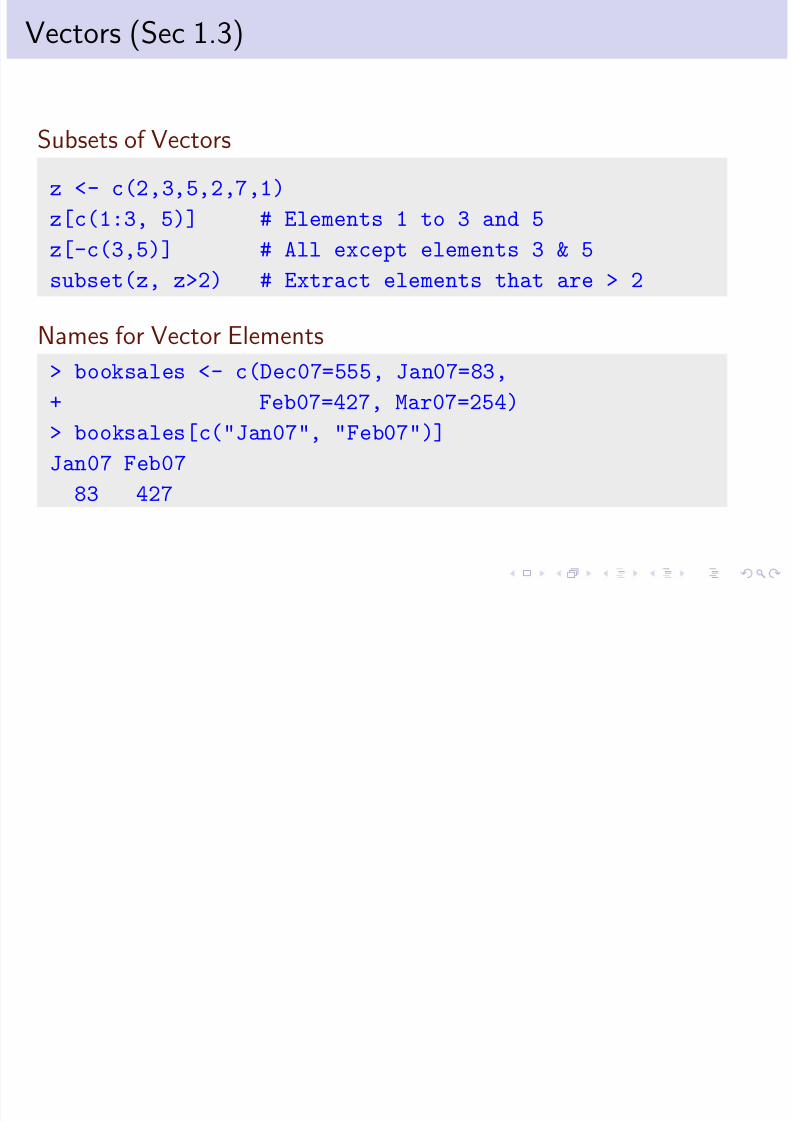
Vectors (Sec 1.3)
Subsets of Vectors
z <- c(2,3,5,2,7,1)
z[c(1:3, 5)] # Elements 1 to 3 and 5
z[-c(3,5)] # All except elements 3 & 5
subset(z, z>2) # Extract elements that are > 2
Names for Vector Elements
> booksales <- c(Dec07=555, Jan07=83,
+ Feb07=427, Mar07=254)
> booksales[c("Jan07", "Feb07")]
Jan07 Feb07
83 427
F ( 5 1 2)

8/6/2019 R Course Overheads
http://slidepdf.com/reader/full/r-course-overheads 19/49
Factors (ss 5.1.2)
Create a character vector
> field <- c("Med", "Lit", "Chem", "Med", "Med")> field
[1] "Med" "Lit" "Chem" "Med" "Med"
# Nobel winners: Katz, White, Comforth, Doherty, Marshall
From field, create the factor fieldfac> fieldfac <- factor(field)
> fieldfac
[1] Med Lit Chem Med Med
Levels: Chem Lit Med
> unclass(fieldfac)[ 1 ] 3 2 1 3 3
attr(,"levels")
[1] "Chem" "Lit" "Med"
Notice that, by default, the levels are taken in alphanumeric order.
Diff t Ki d f F ti (S 1 5 & 14 3)
8/6/2019 R Course Overheads
http://slidepdf.com/reader/full/r-course-overheads 20/49
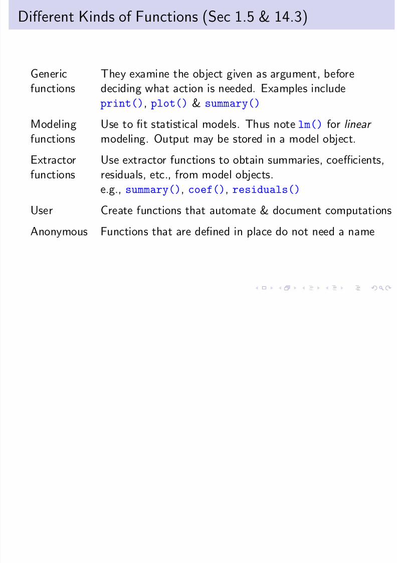
Different Kinds of Functions (Sec 1.5 & 14.3)
Generic They examine the object given as argument, beforefunctions deciding what action is needed. Examples include
print(), plot() & summary()
Modeling Use to fit statistical models. Thus note lm() for linear
functions modeling. Output may be stored in a model object.Extractor Use extractor functions to obtain summaries, coefficients,functions residuals, etc., from model objects.
e.g., summary(), coef(), residuals()
User Create functions that automate & document computations
Anonymous Functions that are defined in place do not need a name
V t U f l F ti
8/6/2019 R Course Overheads
http://slidepdf.com/reader/full/r-course-overheads 21/49
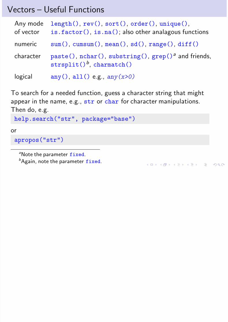
Vectors – Useful Functions
Any mode length(), rev(), sort(), order(), unique(),of vector is.factor(), is.na(); also other analagous functions
numeric sum(), cumsum(), mean(), sd(), range(), diff()
character paste(), nchar(), substring(), grep()a and friends,strsplit()b , charmatch()
logical any(), all() e.g., any(x>0)
To search for a needed function, guess a character string that mightappear in the name, e.g., str or char for character manipulations.Then do, e.g.
help.search("str", package="base")or
apropos("str")
aNote the parameter fixed.b Again, note the parameter fixed.
Functions that create vectors
8/6/2019 R Course Overheads
http://slidepdf.com/reader/full/r-course-overheads 22/49
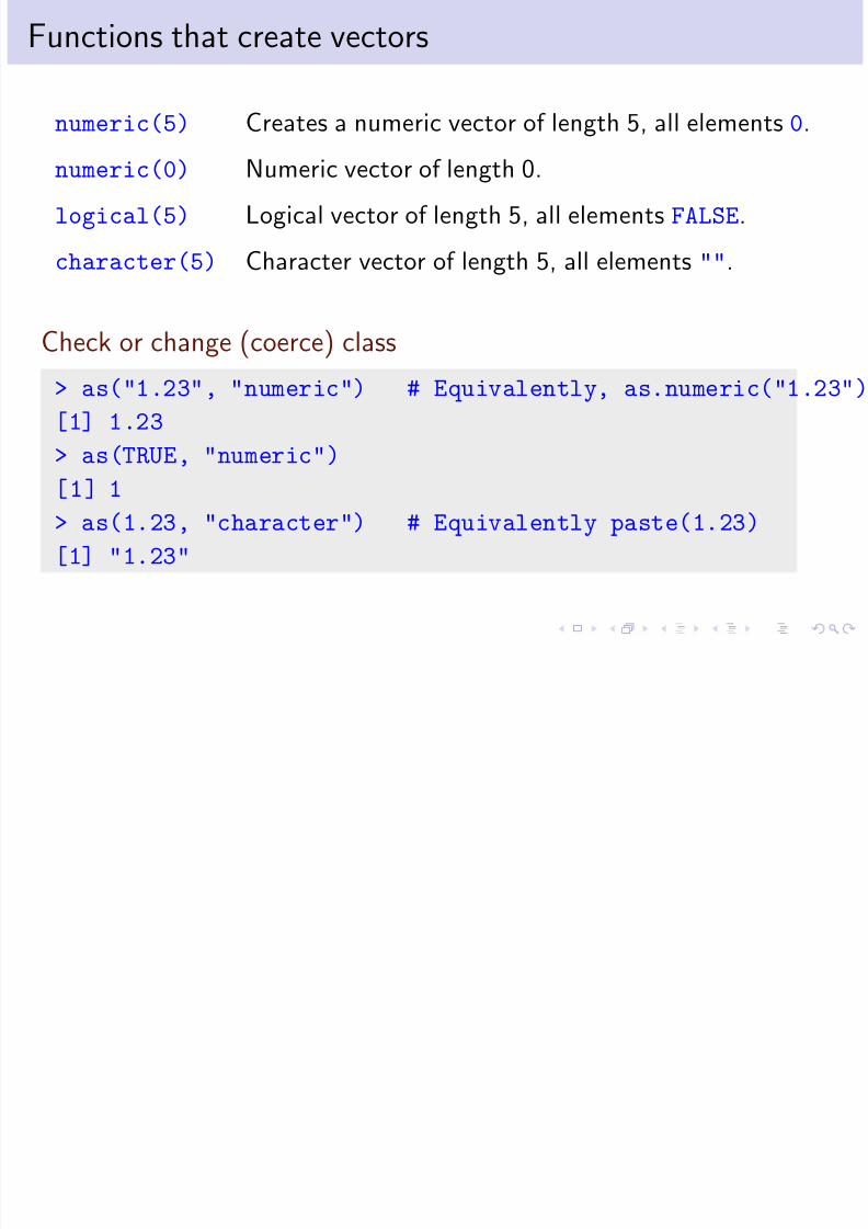
Functions that create vectors
numeric(5) Creates a numeric vector of length 5, all elements 0.
numeric(0) Numeric vector of length 0.
logical(5) Logical vector of length 5, all elements FALSE.
character(5) Character vector of length 5, all elements "".
Check or change (coerce) class
> as("1.23", "numeric") # Equivalently, as.numeric("1.23")
[1] 1.23
> as(TRUE, "numeric")[1] 1
> as(1.23, "character") # Equivalently paste(1.23)
[1] "1.23"
Functions that are useful with data frames (Sec 14 7)
8/6/2019 R Course Overheads
http://slidepdf.com/reader/full/r-course-overheads 23/49
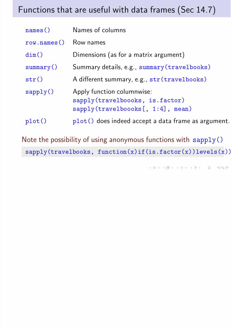
Functions that are useful with data frames (Sec 14.7)
names() Names of columns
row.names() Row names
dim() Dimensions (as for a matrix argument)
summary() Summary details, e.g., summary(travelbooks)
str() A different summary, e.g., str(travelbooks)sapply() Apply function columnwise:
sapply(travelboooks, is.factor)
sapply(travelboooks[, 1:4], mean)
plot() plot() does indeed accept a data frame as argument.
Note the possibility of using anonymous functions with sapply()
sapply(travelbooks, function(x)if(is.factor(x))levels(x))
User defined Functions (ss 14 3 3)
8/6/2019 R Course Overheads
http://slidepdf.com/reader/full/r-course-overheads 24/49
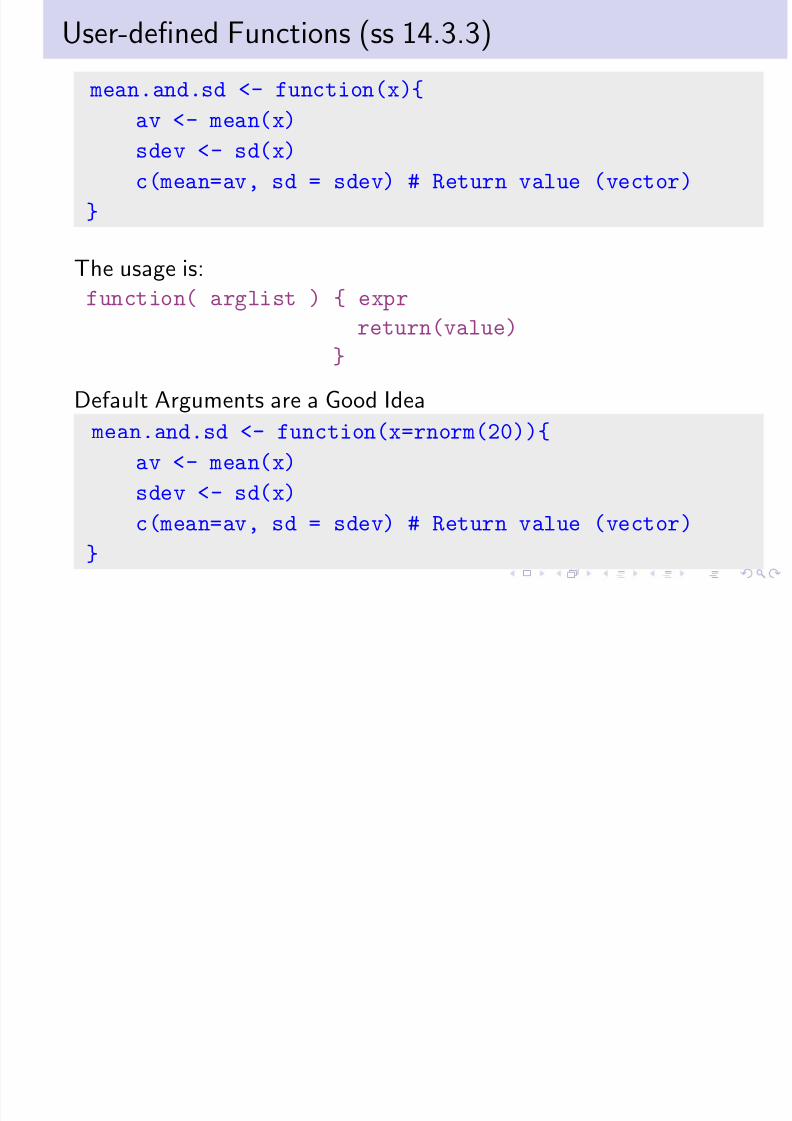
User-defined Functions (ss 14.3.3)
mean.and.sd <- function(x){
av <- mean(x)
sdev <- sd(x)c(mean=av, sd = sdev) # Return value (vector)
}
The usage is:function( arglist ) { expr
return(value)
}
Default Arguments are a Good Idea
mean.and.sd <- function(x=rnorm(20)){
av <- mean(x)
sdev <- sd(x)
c(mean=av, sd = sdev) # Return value (vector)
}
Tables and Cross tabulation (ss 5 4 4); table()
8/6/2019 R Course Overheads
http://slidepdf.com/reader/full/r-course-overheads 25/49
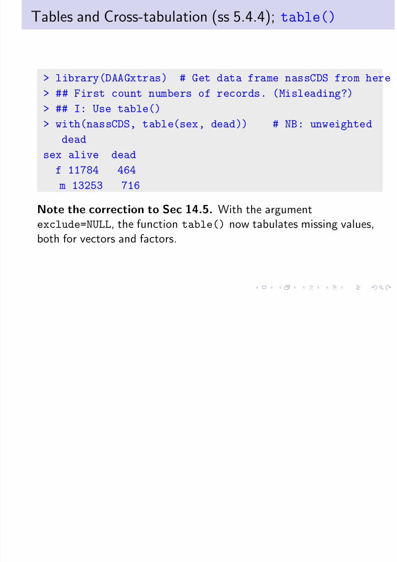
Tables and Cross-tabulation (ss 5.4.4); table()
> library(DAAGxtras) # Get data frame nassCDS from here
> ## First count numbers of records. (Misleading?)
> ## I: Use table()
> with(nassCDS, table(sex, dead)) # NB: unweighted
deadsex alive dead
f 11784 464
m 13253 716
Note the correction to Sec 14.5. With the argumentexclude=NULL, the function table() now tabulates missing values,both for vectors and factors.
Tables and Cross-tabulation (Sec 1 5 & ss 2 2 1 ):

8/6/2019 R Course Overheads
http://slidepdf.com/reader/full/r-course-overheads 26/49
Tables and Cross-tabulation (Sec 1.5 & ss 2.2.1 ):xtabs()
> ## II: Use xtabs()
> xtabs(~ sex + dead, data=nassCDS) # NB: unweighted
. . .
> ## Now weight records a/c 1/(sampling fraction)
> xtabs(weight ~ sex + dead, data=nassCDS)
dead
sex alive dead
f 5899999.64 25677.26 m 6167937.23 39917.87
Review & Additional Points

8/6/2019 R Course Overheads
http://slidepdf.com/reader/full/r-course-overheads 27/49
Review, & Additional Points
Vignettes (ss 14.13.1) are pdf files that accompany packages Saving into and retrieving objects from image files (Sec 1.8 & ss
14.1.2)
Attaching image files (Sec 14.1)
Matrices (5.3) Lists (ss 3.1.3 & Sec 14.7)
User functions (ss 1.5.3 & Sec 14.3)
Common sources of difficulty (5.6).
Next:
Base & Trellis Graphics
Base or “Traditional” Graphics (Sec 1 6 & 14 11)

8/6/2019 R Course Overheads
http://slidepdf.com/reader/full/r-course-overheads 28/49
Base or Traditional Graphics (Sec 1.6 & 14.11)
Base graphics comprises plot() and allied functions
Functions plot(), points(), lines(), text(), mtext(),axis(), identify() etc. form a suite
Choice: old plot(x, y) syntax vs newer plot(y ∼ x) formula syntax:
plot(x, y) with(women, plot(height, weight))
plot(y ∼ x) plot(weight ∼ height, data=women)
par(), etc Use to set parameters in base graphics (Sec 6.2)Some parameters must be set using par()
Specify others in function call. Or there may be a choice.
NB: Some base graphics functions do not take a data parameterOther (mostly 2-D) graphics:
(i) lattice (trellis) graphics, using the lattice package,and (ii) the low-level grid package on which lattice is built.
3-D Graphics: Note rgl , misc3d and tkrplot .
Lattice Graphics (Sec 1 7 & Secx 4 3)

8/6/2019 R Course Overheads
http://slidepdf.com/reader/full/r-course-overheads 29/49
Lattice Graphics (Sec 1.7 & Secx 4.3)
Lattice Lattice is a flavour of trellis graphics
(the S-PLUS flavour was the original implementation)Grid grid is a low-level graphics system. It was used to build lattice .
For grid , see Part II of Paul Murrell’s R Graphics
ggplot2 ggplot2 is an R implementation of Wilkinson’s
Grammar of Graphics . It has some nice features.Lattice Lattice is more structured, automated and stylized.vs base Much is done automatically, without user intervention.
Changes to the default style are harder than for base.
Lattice Lattice syntax is consistent and tightly regulatedsyntax For use of lattice, graphics formulae are mandatory.
latticist The latticist() function in the latticist package opensa simple GUI to the lattice & vcd packages.
Beer+Wine+Spirit, conditioning on Country

8/6/2019 R Course Overheads
http://slidepdf.com/reader/full/r-course-overheads 30/49
Beer Wine Spirit, conditioning on Country
A m o u n t c o n s u m e d ( p e r p e r s o n )
1
2
3
4
5
1998 2000 2002 2004 2006
q q q qq
q
q q q
Australia
1998 2000 2002 2004 2006
qq q
q q q q qq
NewZealand
Beer Spirit Wine
xyplot(Beer+Spirit+Wine ~ Year | Country, data=grog,
outer=FALSE, auto.key=list(columns=3))
NB: Code has been simplified; next slide has full details.
Beer+Wine+Spirit, conditioning on Country, with frills
8/6/2019 R Course Overheads
http://slidepdf.com/reader/full/r-course-overheads 31/49
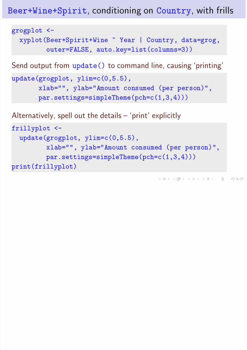
Beer Wine Spirit, conditioning on Country, with frills
grogplot <-
xyplot(Beer+Spirit+Wine ~ Year | Country, data=grog,
outer=FALSE, auto.key=list(columns=3))
Send output from update() to command line, causing ‘printing’
update(grogplot, ylim=c(0,5.5),
xlab="", ylab="Amount consumed (per person)",par.settings=simpleTheme(pch=c(1,3,4)))
Alternatively, spell out the details – ‘print’ explicitly
frillyplot <-update(grogplot, ylim=c(0,5.5),
xlab="", ylab="Amount consumed (per person)",
par.settings=simpleTheme(pch=c(1,3,4)))
print(frillyplot)
Simple Lattice Examples
8/6/2019 R Course Overheads
http://slidepdf.com/reader/full/r-course-overheads 32/49
p p
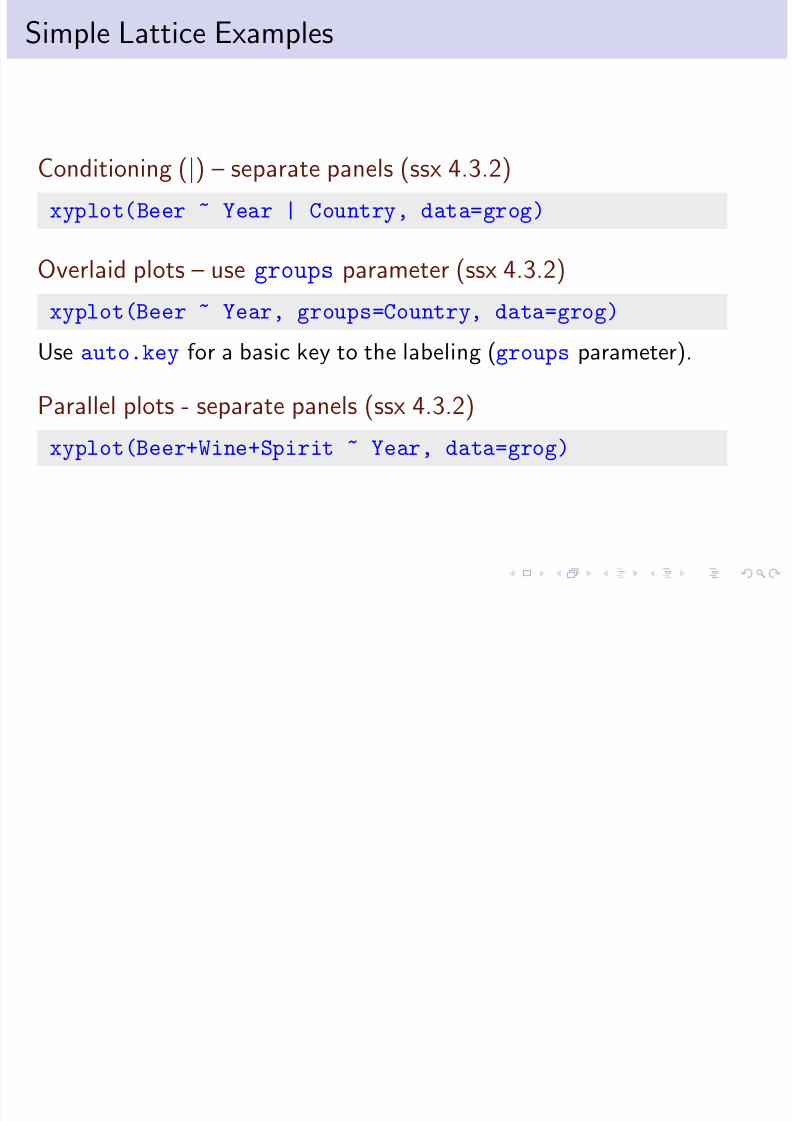
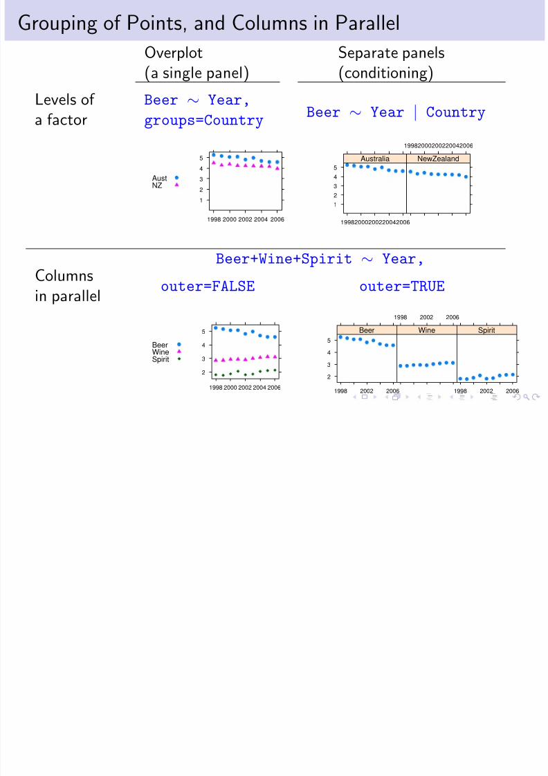
Conditioning (|) – separate panels (ssx 4.3.2)
xyplot(Beer ~ Year | Country, data=grog)
Overlaid plots – use groups parameter (ssx 4.3.2)
xyplot(Beer ~ Year, groups=Country, data=grog)
Use auto.key for a basic key to the labeling (groups parameter).
Parallel plots - separate panels (ssx 4.3.2)
xyplot(Beer+Wine+Spirit ~ Year, data=grog)
Grouping of Points, and Columns in Parallel
8/6/2019 R Course Overheads
http://slidepdf.com/reader/full/r-course-overheads 33/49
p g ,
Overplot(a single panel)
Separate panels(conditioning)
Levels of a factor
Beer ∼ Year,groups=Country
Beer ∼ Year | Country
1
2
3
4
5
1998 2000 2002 2004 2006
q q q qq
qq q q
Aust
NZ
q
12
3
4
5
19982000200220042006
q q q qq q
q q q
Australia
19982000200220042006
qq q q q q q q
q
NewZealand
Beer+Wine+Spirit ∼ Year,Columns
in parallel outer=FALSE outer=TRUE
2
3
4
5
1998 2000 2002 2004 2006
q q q qq
qq q q
BeerWineSpirit
q
2
3
4
5
1998 2002 2006
q q q qqqq q q
Beer
1998 2002 2006
q q q q q q q q q
Wine
1998 2002 2006
q q qqq q
q q q
Spirit
Lattice parameter settings
8/6/2019 R Course Overheads
http://slidepdf.com/reader/full/r-course-overheads 34/49
p g
1. The ‘theme’ determines point and line settings. Changes arereadily made using simpleTheme() (recent version of lattice ).
2. For axis, axis tick, tick label and axis label settings use theargument scales in the function call.
3. Lattice objects can be created, then updated – use update().
4. Note also the arguments layout (# rows × # columns × #pages) and aspect (aspect ratio).
5. The type argument can specify any combination of p (points), l
(lines), b (points & lines), r (regression lines) and smooth (asmooth curve). Set span to control the smoothness of any curve.
Use of simpleTheme() for Point & Line Settings
8/6/2019 R Course Overheads
http://slidepdf.com/reader/full/r-course-overheads 35/49
p g
First use simpleTheme() to create a “theme” with the new settings:
miscSettings <- simpleTheme(pch = 16, cex=1.25)
Alternatives are then:
(i) Supply the “theme” to par.settings in the function call.[This stores the settings with the object. These
stored settings over-ride the global settings at the time of printing.]xyplot(Beer ~ Year | Country, data=grog,
par.settings=miscSettings)
(ii) Supply the “theme” to trellis.par.set(), prior to plotting:
[Makes the change globally, until a new trellis device is opened]trellis.par.set(miscSettings)
xyplot(Beer ~ Year | Country, data=grog)
Axis, tick, tick label and axis label settings

8/6/2019 R Course Overheads
http://slidepdf.com/reader/full/r-course-overheads 36/49
jobplot <- xyplot(Ontario+BC ~ Date, data=jobs)
## Half-length ticks, each quarter, Label years, Add key
tpos <- seq(from=95, by=0.25, to=97)tlabs <- rep(c("Jan95", "", "Jan96", "", "Jan97"),
c(1,3,1,3,1))
update(jobplot, auto.key=list(columns=2), xlab="",
scales=list(tck=0.5, x=list(at=tpos, labels=tlabs)))
Date
O n t a r i o + B C
2000
3000
4000
5000
95.0 95.5 96.0 96.5 97.0
qqqqqqqqqqqqqqqqqqqqqqqq
qqqqqqqqqqqqqqqqqqqqqqqq
O n t a r i o +
B C
2000
3000
4000
5000
Jan95 Jan96 Jan97
q qqq qqq qqq qq qqq qqqqqq qq q
q qqq qqq qqq qq qqq qqq qqq qq q
Ontario BC q
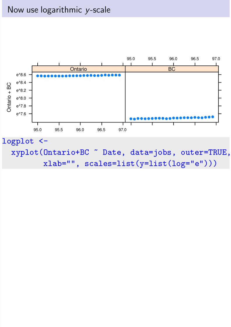
Now use logarithmic y -scale
8/6/2019 R Course Overheads
http://slidepdf.com/reader/full/r-course-overheads 37/49
O n t a r i o + B C
e^7.6
e^7.8
e^8.0
e^8.2
e^8.4
e^8.6
95.0 95.5 96.0 96.5 97.0
q q q q q q q q q q q q q q q q q q q q q q q q
Ontario
95.0 95.5 96.0 96.5 97.0
q q q q q q q q q q q q q q qq q q q q q q q q
BC
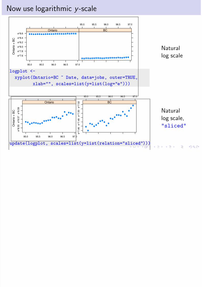
logplot <-xyplot(Ontario+BC ~ Date, data=jobs, outer=TRUE,
xlab="", scales=list(y=list(log="e")))
Naturallog scale
O n t a r i o + B C
e ^ 8 . 5
5
e ^ 8 . 5
7
e ^ 8 . 5 9
95.0 95.5 96.0 96.5 97.0
q q
qq q q q q
q
q qq q
q q qq q
q
q
q
q qq
Ontario
95.0 95.5 96.0 96.5 97.0
e ^ 7 . 4
6
e ^ 7 . 4
8
e ^ 7 . 5
0
e ^ 7 . 5
2
q
q
q
q qq
q
q
q q
q
q q q
q
q
q
q
BC
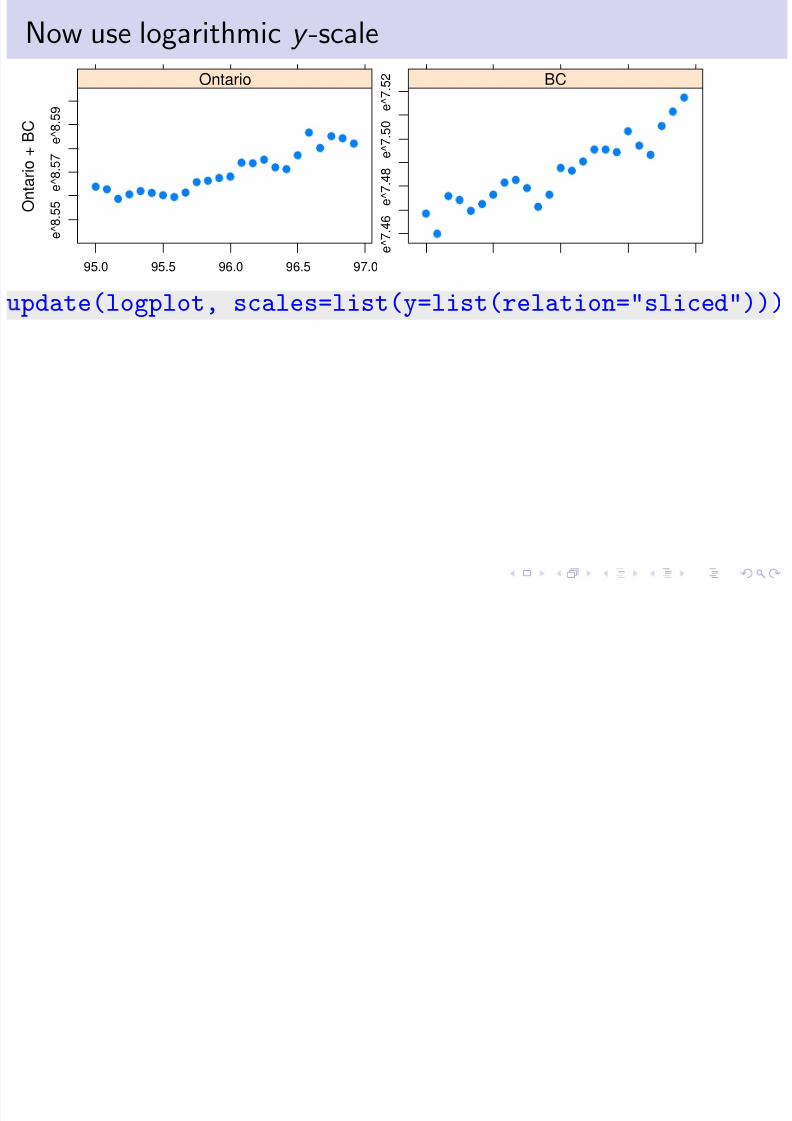
update(logplot, scales=list(y=list(relation="sliced")))
Naturallog scale,"sliced"
Now use logarithmic y -scale
8/6/2019 R Course Overheads
http://slidepdf.com/reader/full/r-course-overheads 38/49
O n t a r i o + B C
e^7.6
e^7.8
e^8.0
e^8.2
e^8.4
e^8.6
95.0 95.5 96.0 96.5 97.0
q q q q q q q q q q q q q q q q q q q q q q q q
Ontario
95.0 95.5 96.0 96.5 97.0
q q q q q q q q q q q q q q qq q q q q q q q q
BC
logplot <-
xyplot(Ontario+BC ~ Date, data=jobs, outer=TRUE,
xlab="", scales=list(y=list(log="e")))
Now use logarithmic y -scale
8/6/2019 R Course Overheads
http://slidepdf.com/reader/full/r-course-overheads 39/49
O n t a r i o +
B C
e ^ 8 . 5
5
e ^ 8 . 5
7
e ^ 8 . 5
9
95.0 95.5 96.0 96.5 97.0
q q
qq q q q q
q
q qq q
q q qq q
q
q
q
q qq
Ontario
e ^ 7 . 4
6
e ^ 7 . 4
8
e ^
7 . 5
0
e ^ 7 . 5
2
q
q
q
q qq
q
q
q q
qq q q
q
q
q
q
BC
pdate(logplot, scales=list(y=list(relation="sliced")))
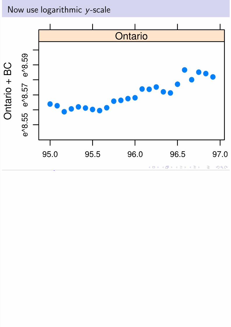
Now use logarithmic y -scale
8/6/2019 R Course Overheads
http://slidepdf.com/reader/full/r-course-overheads 40/49
O n t a r i o +
B C
e ^ 8 .
5 5
e ^ 8 . 5 7
e ^ 8 . 5
9
95.0 95.5 96.0 96.5 97.0
q q
qq q q q q
q
q qq q
q q qq q
q
q
q
q qq
Ontario
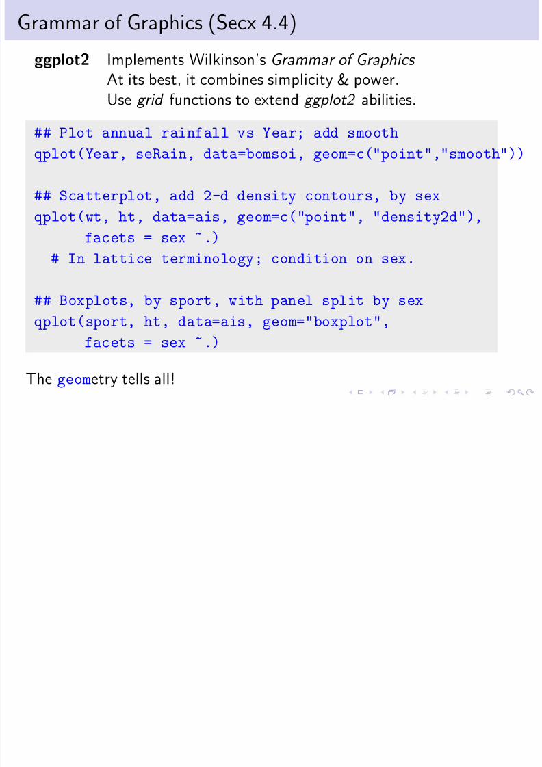
Grammar of Graphics (Secx 4.4)
8/6/2019 R Course Overheads
http://slidepdf.com/reader/full/r-course-overheads 41/49
ggplot2 Implements Wilkinson’s Grammar of Graphics
At its best, it combines simplicity & power.
Use grid functions to extend ggplot2 abilities.
## Plot annual rainfall vs Year; add smooth
qplot(Year, seRain, data=bomsoi, geom=c("point","smooth"))
## Scatterplot, add 2-d density contours, by sexqplot(wt, ht, data=ais, geom=c("point", "density2d"),
facets = sex ~.)
# In lattice terminology; condition on sex.
## Boxplots, by sport, with panel split by sex
qplot(sport, ht, data=ais, geom="boxplot",
facets = sex ~.)
The geometry tells all!
Linear Models, in the style of lm() (Ch 6 & Chx 3)

8/6/2019 R Course Overheads
http://slidepdf.com/reader/full/r-course-overheads 42/49
Linear model Any model that lm() will fit is a “linear” model.lm() can fit highly non-linear forms of response!
Diagnostic Use plot() with the model object as argument,plots to get a basic set of diagnostic plots.
termplot() If there are no interaction terms, use termplot() tovisualize the contributions of the different terms.
(Why are interactions a problem for lm()?)Factors In model terms, use factors to model qualitative effects.
Model How should coefficients be interpreted? Examine thematrices model matrix. (This is an especial issue for factors.)
GLMs Generalized Linear Models are an extension of linearmodels, commonly used for analyzing counts.
[NB: lm() assumes independently & identically distributed (iid) errors,perhaps after applying a weighting function.]
Models with Non-iid Errors (Ch 9 & Ch 10)
8/6/2019 R Course Overheads
http://slidepdf.com/reader/full/r-course-overheads 43/49
Error Term Errors do not have to be (and often are not) iidMulti-level Multi-level models are a (relatively) simple type of non-iidmodels model. Fit using lme() (nlme ) or lmer() (lme4 package).
Such models allow different errors of prediction, dependingon the intended prediction. (The error term does matter!)
aov models For suitably balanced designs, these give theinformation needed for a multi-level type of analysis.[See Chapters 4 & 7 of DAAGUR]
Time Points that are close together in time are likely to show aseries (usually, positive) correlation. R’s acf() and arima()
functions are highly useful tools for time series.
Multivariate Models and Methods (Ch 12)
8/6/2019 R Course Overheads
http://slidepdf.com/reader/full/r-course-overheads 44/49
Ordination Principal components, multi-dimensional scaling [D-Ch 12]
Multivariate distances – do variables have equal weight?Phylogenetics – distances are from evolutionary model.
2D or 3D Ordination may allow a low-dimensional view.views Which view is best, or which is the “right” view
NB: The “view” can be rotated arbitrarily.
Classification Linear Discriminant Analysis [D-Ch 12]: simple.methods Trees [D-Ch 11]: simple to fit; may be hard to interpret.
Random forests [Ch 11]: easy to fit, superior to trees?
Neural nets, SVMs: Watch for exaggerated claims!Classify, then A clear criterion determines the distance measure.ordinate Different classifications will give different axes (views).
Ordination (ss 12.1.2 & 12.1.3)
8/6/2019 R Course Overheads
http://slidepdf.com/reader/full/r-course-overheads 45/49
Road Distances example
Can we recover the geographical configuration?
Calculate distances from points in n-space
Is a “good”representation possible in dimension 2 or 3?
NB: How should variables be weighted? Equally?
Phylogenetics
Distances should reflect time from Last Common Ancestor!
C.f. the dist.dna() function in ape . Choose between:raw, JC69, K80 (default), F81, K81, F84, BH87, T92, TN93, GG95,logdet, & paralin.
Different models for evolutionary imply different distances.
There may not be a unique distance between two organisms.
Classification (Ch 11 & Sec 12.2)
8/6/2019 R Course Overheads
http://slidepdf.com/reader/full/r-course-overheads 46/49
Linear Methods (ss 12.2)
The notes have examples of the use of lda() and qda(), both fromthe MASS package.
Tree-based Methods (Ch 11)
These are about as non-parametric as is possible – a strong contrastwith lda() and qda(). The notes demonstrate the use of rpart()
which generates trees, and of randomForest() which generates
forests of trees. The functions take their names from the packages inwhich they are the main workhorses.
Key Language Ideas (Sec 14.8 & 14.9)
8/6/2019 R Course Overheads
http://slidepdf.com/reader/full/r-course-overheads 47/49
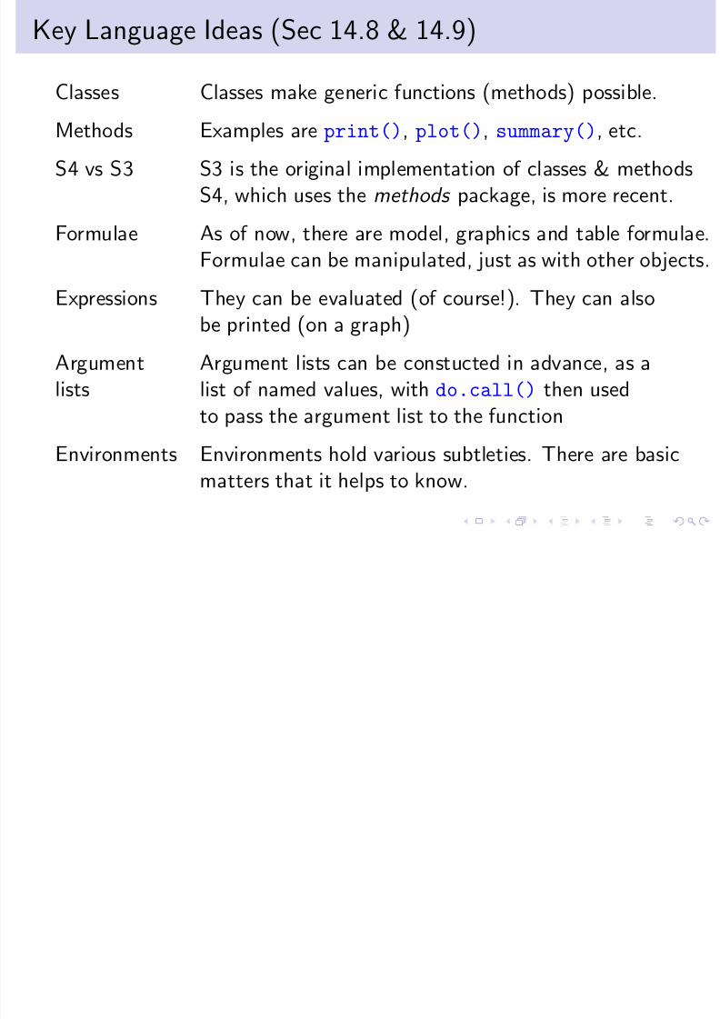
Classes Classes make generic functions (methods) possible.
Methods Examples are print(), plot(), summary(), etc.S4 vs S3 S3 is the original implementation of classes & methods
S4, which uses the methods package, is more recent.
Formulae As of now, there are model, graphics and table formulae.
Formulae can be manipulated, just as with other objects.Expressions They can be evaluated (of course!). They can also
be printed (on a graph)
Argument Argument lists can be constucted in advance, as a
lists list of named values, with do.call() then usedto pass the argument list to the function
Environments Environments hold various subtleties. There are basicmatters that it helps to know.
8/6/2019 R Course Overheads
http://slidepdf.com/reader/full/r-course-overheads 48/49
THE END
8/6/2019 R Course Overheads
http://slidepdf.com/reader/full/r-course-overheads 49/49
You may think that this is the end,
Well it is, but to prove we’re all liars,
We’re going to sing it again,
Only this time we’ll sing a little higher.
Actually, this is not the end, for there are many other analysis methodsand R packages to explore, even if not in this workshop!