Scho

olof

Mat

hem

atic

sU

nive

rsit

yof

Nai

robi

ISSN: 2410-1397

Master Project in Actuarial Science

RANGE-BASED APPROACH TO VOLATILITYMODELLING AND FORECASTING VALUE-AT-RISK

Research Report in Mathematics, Number 20, 2020

FRANCIS MAKORI NYAMACHE June 2020

Submi�ed to the School of Mathematics in partial fulfillment for a degree in Master of Science in Actuarial Science

Master Project in Actuarial Science University of NairobiJune 2020

RANGE-BASED APPROACH TO VOLATILITYMODELLING AND FORECASTING VALUE-AT-RISKResearch Report in Mathematics, Number 20, 2020

FRANCIS MAKORI NYAMACHE

School of MathematicsCollege of Biological and Physical sciencesChiromo, o� Riverside Drive30197-00100 Nairobi, Kenya

Master ThesisSubmi�ed to the School of Mathematics in partial fulfillment for a degree in Master of Science in Actuarial Science

Submi�ed to: The Graduate School, University of Nairobi, Kenya

ii

Abstract

The purpose of this thesis is to model and forecast value-at-risk based on range-measuring

rather than the commonly acknowledged volatility models that are based on closing prices.

The use of close-to-close prices in modelling and forecasting value-at-risk might not cap-

ture important intra-day information about the price movement. As a result, crucial price

movement information is lost and consequently the model becomes less e�cient. This

thesis recommends the inclusion or range-measuring, described as the di�erence between

the highest and lowest prices of an underlying stock within a time interval, a day, to com-

pute Value-at-Risk. The project uses data of an NSE-listed and trading company, SASN,

between November 2009 and November 2019 on which the predictability of range-based

and close-to-close estimates was established. It was observed that the values obtained

by range-based models were more accurate than when only the daily closing prices are

used. The range-based models successfully capture dynamics of the volatility and achieves

improve performance relative to the GARCH-type models. These �ndings are fairly con-

sistent and can be extended to applications like portfolio optimization.

Master Thesis in Mathematics at the University of Nairobi, Kenya.ISSN 2410-1397: Research Report in Mathematics©FRANCIS MAKORI NYAMACHE, 2020DISTRIBUTOR: School of Mathematics, University of Nairobi, Kenya

iv

Declaration and Approval

I the undersigned declare that this dissertation is my original work and to the best of my

knowledge, it has not been submitted in support of an award of a degree in any other

university or institution of learning.

Signature Date

Francis M. Nyamache

Reg No. I56/12745/2018

In my capacity as a supervisor of the candidate’s dissertation, I certify that this dissertation

has my approval for submission.

Signature Date

Prof. Philip Ngare

School of Mathematics,

University of Nairobi,

Box 30197, 00100 Nairobi, Kenya.

E-mail: pngare@uonbi.ac.ke

AcknowledgmentMy deepest gratitude to God for giving me strength, courage, knowledge, and wisdomto be able to get all that was needed for the completion of this program. He provided mewith all that I needed through supportive parents, mentors and friends. Completing theMasters program has been my greatest achievement towards achieving my professionalcareer. I greatly appreciate my supervisor Prof. Philip Ngare, whose contributionand constructive criticism helped me put more effort to make this work original. Myutmost regard goes to my parents who with great care, thoroughness and with sacrificelaid a foundation for my education. I am and will forever be grateful to my beginningteachers, mentors, and friends who encouraged and supported my journey this far, andmade this achievement possible.

Table of Contents

1 Introduction 1

1.1 Background of the Study . . . . . . . . . . . . . . . . . . . . . . . . 1

1.2 Justification of the Study . . . . . . . . . . . . . . . . . . . . . . . . 3

1.3 Statement of the Problem . . . . . . . . . . . . . . . . . . . . . . . . 3

1.4 Hypothesis of the Study . . . . . . . . . . . . . . . . . . . . . . . . . 4

1.5 Objectives of the study . . . . . . . . . . . . . . . . . . . . . . . . . 5

1.6 Significance of the Study . . . . . . . . . . . . . . . . . . . . . . . . 5

2 Literature Review 7

3 Methodology 12

3.1 Introduction . . . . . . . . . . . . . . . . . . . . . . . . . . . . . . . 12

3.2 GARCH and TARCH Models) . . . . . . . . . . . . . . . . . . . . . 13

3.3 Range-Based Volatility . . . . . . . . . . . . . . . . . . . . . . . . . 14

3.4 Evaluating the Volatility Forecast . . . . . . . . . . . . . . . . . . . . 16

3.5 Estimating and Validating Value-at-Risk . . . . . . . . . . . . . . . . 17

Acknowledgement v

Table of Contents vi

List of Tables viii

List of Figures ix

Declaration iv

List of Abbreviations and Acronyms xi

Abstract ii

4 Data Analysis and Results 21

4.1 Introduction . . . . . . . . . . . . . . . . . . . . . . . . . . . . . . . 21

4.2 Descriptive Statistics . . . . . . . . . . . . . . . . . . . . . . . . . . 21

4.3 MSE and QLIKE Loss Functions . . . . . . . . . . . . . . . . . . . . 27

4.4 Diebold-Mariano Test . . . . . . . . . . . . . . . . . . . . . . . . . . 27

4.5 Interpretation of Results . . . . . . . . . . . . . . . . . . . . . . . . 30

5 Conclusions and Recommendations 33

5.1 Conclusions . . . . . . . . . . . . . . . . . . . . . . . . . . . . . . . 33

5.2 Recommendations . . . . . . . . . . . . . . . . . . . . . . . . . . . 34

5.3 Room for Further Research . . . . . . . . . . . . . . . . . . . . . . . 34

References 35

Appendices 38

List of Tables

1.1 NSE-listed Company Data . . . . . . . . . . . . . . . . . . . . . . . 3

4.1 Descriptive Statistics SASN returns & Volatility . . . . . . . . . . . . 21

4.2 The Table details return and range-based volatility model estimates forSASINI, 2009-2019 . . . . . . . . . . . . . . . . . . . . . . . . . . . 26

4.3 At 5 % significance level. MSE & QLIKE assessment for volatilityforecasting, ranked from best-performing to least . . . . . . . . . . . 27

4.4 At 5% significance level. Diebold-Mariano Test for volatility forecasting 28

4.5 The Table details the Violation rate, ASMF, unconditional and condi-tional Likelihood ratio test . . . . . . . . . . . . . . . . . . . . . . . 28

List of Figures

4.2.1 The time series plot above shows clustering characteristics of returns.High in certain periods and low in certain periods, evolving over theperiod under study exhibiting a continuous manner and hence volatil-ity. Use of log returns will help achieve stationarity. . . . . . . . . . . 22

4.2.2 Ljung-Box Q Statistics ACF range series . . . . . . . . . . . . . . . . 23

4.2.3 SASN Range Series Returns . . . . . . . . . . . . . . . . . . . . . . 24

4.2.4 SASN Daily Series Returns . . . . . . . . . . . . . . . . . . . . . . . 24

4.2.5 SASN Close-to-Close Volatility Series Returns . . . . . . . . . . . . 25

4.2.6 SASN Garman Klass Volatility Series . . . . . . . . . . . . . . . . . 25

4.4.1 Actual & Forecasted Volatility Plot, RGARCH Model . . . . . . . . . 29

4.4.2 RGARCH Model fitting plots. Different gaphs we obtained for 4-yearsahead forecasts . . . . . . . . . . . . . . . . . . . . . . . . . . . . . 29

4.4.3 Comparison of 1-step-ahead volatility forecasts for the competing models 30

4.4.4 CARR Model, 1-step-ahead forecasts . . . . . . . . . . . . . . . . . 30

4.4.5 RGARCH Model, 1-step-ahead forecasts . . . . . . . . . . . . . . . . 31

List of Abbreviations and Acronyms

AIC Akaike Information Criterion

ASMF Average Square Magnitude function

BIC Bayes Information Criterion

CARR Conditional Autoregressive Range

CDF Cumulative distribution function

DCF Conditional Density Function

KCB Kenya Commercial Bank

GARCH Generalized Autoregressive Conditional Heteroscedasticity

ME Mean Error

MSE Mean-Square Error

NSENairobi Stock Exchange

RGARCH Range Generalized Autoregressive Conditional Heteroscedasticity

RTARCH Range Threshold Generalized Autoregressive Conditional Heteroscedastic-ity

TARCH Threshold Generalized Autoregressive Conditional Heteroscedasticity

QLIKE QLIKE Loss Function

SASN Sasini

VR Violation Ratio

Chapter 1

Introduction

1.1 Background of the Study

Volatility of assets plays a vital role in finance. As a measure of riskiness, volatilityis key in asset pricing, derivatives pricing, risk management, and portfolio manage-ment. A good understanding of return volatilities and accurate estimates are valuableto practitioners in the financial field as well as players in the financial field includingindependent investors and traders.

In the recent, a number of banks have collapsed in Kenya as well as retail companieswhich have significantly impacted the portfolio stability of investment banks and pri-vate investors. Poor risk management and lack of proper oversight, regulation, andassessment of the financial sector have been cited as among the major factors that con-tributed to the collapse of these banks. Gathaiya [2017] established that CBK had putmore focus on macro-prudential regulation that relates to factors affecting individualbanks while giving less focus on factors affecting stability of the entire financial sec-tor. Accurate volatility estimates are essential in the stability of financial institutionsespecially banks plagued with non-performing loans. For instance, Dubai Bank wasput under receivership because of its deteriorating cash reserve ratio Gathaiya [2017].

Due to such failures of investment banks and financial institutions, the need to modeland forecast volatility more accurately has risen gradually, with the aim that accuratevolatility estimates can help. The need for accurate volatility estimates has also grownas the financial markets around the world move towards deregulation and globaliza-tion. This includes entry into financial markets in developing countries and emergingmarkets especially by foreign investors who are much interested in the stability ofthe financial markets and the entire economy. The input into the global risk manage-

1

ment models has therefore continued to grow and the threat of global spillover effectsenlarges due to the use of inaccurate volatility estimates. Volatility quantifies the dis-persion of returns. However, volatility is time-varying and not easy to predict becausevolatility is not observable, and the volatility forecasts are affected by changing esti-mates of the levels of volatility at the time period.

Kenya as an emerging market has attracted significant attention from investors andconsequently practitioners and researchers in the financial field. Kenya’s stock in-dices have yielded high returns becoming appealing and decoupling in demand frominvestors. However, the returns are not consistent hence the need to establish a volatil-ity model that is appropriate for the Kenyan stock market. Kenya offers more excitinglong-term investment opportunities which encourages the analysis of stock market datawith the range-based models to establish whether the range-based model provides moreaccurate forecasts.

1.1.1 Risk Diversification

Geographic diversification of assets is an important requirement in minimizing riskexposure in stock portfolios or pension funds chou. The low correlation between theemerging markets and developed markets have attracted foreign investors to the emerg-ing markets Sharma et al. [2016]. The classical time series models such as the Gen-eralized Autoregressive Conditional Heteroscedasticity (GARCH) models, stochasticsvolatility models, and the implied volatility measures like realized volatility are com-monly used in forecasting volatility. GARCH-type models are used to model time-varying conditional volatility due to their simplicity and easy approach to estimationad flexibility in terms of volatility dynamics.

GARCH-type models are developed using data on closing prices, that is, the dailyreturns. This way, important information about intraday price movement might beneglected. For instance, if the closing price of two consecutive days is equal, thereturn is be zero. Howver, the changes in prices during the day might be explosive andthe typical GARCH model fails to capture this information. Also, the GARCH-typemodels are based on the moving averages with weights that decay gradually hence slowto adapt the changes in levels of volatility Sharma et al. [2016]. Some studies attemptto overcome this drawback using intraday GARCH models. A simpler approach tomodeling the intraday variation is the use of price range. Range is defined as thedifference between the highest and lowest prices over a given sampling interval suchas daily or weekly. This paper uses the day-to-day variability Sharma et al. [2016].The estimates obtained using range apporach are more effective compared to estimatesobtained using the close-to-close return approach.

2

1.2 Justification of the Study

Financial institutions including investment banks, individual and corporate investorsrely on volatility estimates to make investment decisions. Knowing the accuracy ora measure is crucial. For instance, they use Value-at-Risk to estimate the amount ofcash they require to reserve for covering potential losses. While the historical VaR isextremely simple to calculate and explain even to non-risk professionals, it comes withits shortcomings. Banks for instance combine portfolio sensitivity to market changesand probability of a given change in the market to measure market risk. This makesthe need for accurate estimates crucial. Any inaccuracies will imply that the institu-tion is not reserving sufficiently for potential losses. Currently, there is no study thathas covered range-based volatility and empirically tested using of an NSE-listed andtrading company data. This study attempts to fill up the research gap.

In the recent past, banks in Kenya has been put under receivership. [Gathaiya, 2017],established that poor risk management and poor financial sector oversight as amongthe major reasons contributing collapse of Banks such as Imperial Bank, Dubai Bank,and Chase Bank. A research is required to establish better and more accurate volatilitymeasures enabling players in the financial market have a better oversight and improvedrisk management strategies. This research, being the first of the kind in Kenya, will seta foundation for further research and give it the required attention.

Hence, evaluation of volatility using NSE-trading company data could provide an out-look of how the Indices and entire economy is performing. It will give an insight intofurther research and application of the volatility approach recommended in this paperto the entire market.

Table 1.1 shows details of the selected company, category as listed in the NSE, and thestock ticker:

No. Company Names and Stock Ticker Category1. Sasini Ltd (SASN) Agricultural

Table 1.1: NSE-listed Company Data

1.3 Statement of the Problem

Accurate volatility estimates are vital in financial applications such as portfolio opti-mization, derivatives and options pricing. The historical volatility estimators that arecommonly used are less accurate. While other markets, developed economies, havetested range-based models and forecasting on the stock prices, there is little researchon the same in emerging markets. The widely used and well-established return-based

3

volatility measured used in time series analysis such as development of GARCH-typemodels suffer inefficiency. The first challenge with historical models arises from thefact that volatility is not directly observable hence need to address the problem ofvolatility measurement.

Based on the price returns over several days, we obtain volatility of the stock returnswhich is typically defined as the squared returns or standard deviation of the returns.This approach only helps obtain the average volatility over the sampled time periodhence not sufficient since the volatility changes on daily basis. If close-to-close pricesare used to estimate volatility on daily basis, the estimate is referred to as the squareddaily return. Squared daily return is noisy. Since it is the only that we have, it is com-monly used in models such as GARCH-type in which the squared returns are used andprocessed by applying the moving average. If there is a high frequency of intraday datafor whole price process for the day, it is possible to estimate daily volatility. For mostfinancial data, the highest and lowest daily prices are available. Range-based volatil-ity estimation seeks to address the shortcomings of the squared return and standarddeviation approaches to estimating volatility.

The growing need for accurate volatility estimators, need for application on empiricaldata in emerging markets such as Kenya motivated the evaluation whether range pro-vides additional information to the volatility process helpful in improving forecastingcompared to the GARCH-type approaches. One benefit of utilizing the range approachis that the financial assets contain useful information about the movement of priceswithin a given time period whereas the use of squared return only include the closingprices. This is an important feature especially when the market experiences large priceswings Chou and Wang [2014]. The interest to study the application of range-basedapproach to volatility forecasting has grown tremendously in finance literature in de-veloped markets. However, the areas has not be widely explored in emerging markets.The linkages in markets may change due to a financial crisis and volatility is viewedas a vital channel for the changes. Because of market linkages, financial crises signif-icantly spread and impact financial economies on a global scale. We use the range-based volatility model introduced by Chou and Wang [2014] to evaluate changes involatility dependence structure.

1.4 Hypothesis of the Study

Return based volatility estimation uses the open, close and adjusted close prices tocalculate returns while range-based volatility approach uses the difference betweenhighest and lowest stock prices. The open close price can be very low and the open

4

price in the next trading day be high due to market conditions. However, if in theprevious trading day there was a price slump during the day, then there might be marketplayers who are significantly impacted if they transacted when the price was at a thelowest.

This study hypothesizes that range-based volatility approach can guard the marketplayers from such price slumps. Another null hypothesis is that range-based volatilityapproach gives a better estimate of volatility compared to return-based VaR approach.It is also hypothesized that range provides additional intraday information about themovements of stock prices during the day.

1.5 Objectives of the study

Majority of past research studies have focused on return-based volatility estimatorsevident from their wide application in the finance and investment field. For researchstudies involving range-based volatility approach, the researchers have focused on de-veloped markets such as Europe and America. Although emergent markets such asKenya present exciting long-term investment opportunities, there is no research thathas empirically tested the Kenyan stock market using the range-based volatility esti-mators.

1.5.1 General Objective

The general objective of this study is to test the range-based volatility estimation usingdata of a company listed and trading at the NSE.

1.5.2 Specific Objectives

The Specific objectives of this study are:

1. To test the accuracy of range-based volatility model in the Kenyan market byestablishing whether the approach provides additional information.

2. To assess which among the range-based models, RGARCH and CARR is betterthan the other.

1.6 Significance of the Study

This study uses data from the Kenyan stock market to assess the accuracy of range-based volatility models. An accurate measure of volatility will be significant to the

5

different stakeholders in the financial sector including savings and investment banksand institutions, traders in the stock market, and individual investors. The findingsof the study will not only be applicable to the stock exchange but also in the entirefinancial sector benefiting corporations as well as individuals.

With this study, practitioners in the financial sector can blend its concepts and find-ing with technology to further financial technology such as development of virtualinvestment advisors. The findings of the study will benefit practitioners in the financialsector. Banks and financial institutions will use the findings to develop improved riskmanagement strategies. With more accurate value at risk estimates, financial institu-tions such as banks will be able to allocate sufficient capital for reserves to cover forpotential losses.

6

Chapter 2

Literature Review

It is conventional that asset returns take a normal distribution. However, carrying outa joint multivariate distribution test gives misleading conclusion about the dependenceof assets. Because of the variations in behavior of assets returns during different peri-ods than normal periods, proper asset allocation and even hedging may not be enoughto protect asset returns against unexpected losses Li and Hong [2011]. Various re-searchers have studies extreme risks using different return-based volatility models forthe stock market while little research exists for range-based models in emerging mar-kets such as Kenya. Various research studies in range-based volatility models haveshown better performance than return-based models. Parkinson (1980) in his researchon measurement of errors in return-based volatility estimates established that the errorswere higher and hence yielded to inefficiency of the model. These findings supportedthe desire to investigate whether range provides additional information on price move-ments and how it can be applied in the Kenyan market. In another research conductedby Brandt and Jones [2002] to investigate ranged-based volatility approach to measur-ing volatility using stochastic models reported improved efficiency and robustness tomarket microstructure noise.

Andersen et al. [2003] conducted a research on modeling and forecasting realizedvolatility using high-frequency intraday data. The researchers developed links betweenrealized volatility and conditional variance with the aim of establishing whether themodels could predict volatility with higher accuracy and hence helpful in the currencyexchange market. By treating volatility as observed rather than latent, the approach fa-cilitated the modeling and forecasting with the use of simple methods that are based ondirectly observable variables Andersen et al. [2003]. Guided by the general theory forcontinuous-time arbitrage-free price processes, the researchers developed a forecast-ing framework for realized volatility and correlation. The study established that the

7

range-based framework produced successful volatility estimates and generally domi-nating the estimates from conventional GARCH and related approaches. Additionally,the forecasts were well-calibrated and associated with VaR for multivariate foreign ex-change applications. Volatility forecasts are not only useful in practical financial deci-sions but they extend beyond risk modeling and management into sport and derivativeasset prices Andersen et al. [2003]. The researchers recommended that further studiesexplore the gains achieved by simple volatility modeling and forecasting proceduresthat rely on range.

Research by Brandt and Jones [2006] supports the literature by Andersen et al. [2003].Brandt and Jones [2006] studying range-based exponential GARCH (EGARCH) estab-lished that the range-based model performed better compared to return-based EGARCHmodels for both in-sample and out-of-sample volatility estimates. In their research,Brandt and Jones combined two-factor EGARCH models with data on the range andused empirical analysis of SP 500 index to investigate model superiority based onefficiency of the forecasts. The researchers established that range incorporated in-formation into EGARCH models which significantly improved in-sample fit and theaccuracy of out-sample forecasts of the models. In a two-factor and fractionally in-tegrated EGARCH models, range incorporated volatility asymmetry that dominatedboth in-sample and out-of-sample forecasts. The research also established that log re-turns are more likely to give rise to biased estimates than log range returns becausereturn-based log has idiosyncratic noise.

In another research, Petneházi and Gáll [2019] studied how predictable the range-basedestimates could be. The results were compared against those obtained using close-to-close returns, commonly applicable in practice. Testing the models using Dow JonesIndustrial Average index, the researchers established that the direction of changes inthe estimates obtained using range-based models were more predictable than that of thereturn-based values. Petneházi and Gáll [2019] outlines known properties of volatil-ity which include persistence, mean reversion, asymmetric effect, and influence ofexogenous variables. According to these features of volatility, volatility should beforecastable. However, since it cannot be measured, developing reasonable proxies isthe best approach. Such proxies include the standard deviation of returns calculatedusing daily closing prices. However, following the daily closing prices, it is not possi-ble to tell the price movements during the day which are not captured by close prices.The Open, Close, High, and Low price data is readily available unlike high freqeuencydata such as minutely or hourly price quotes. Although finding accurate volatility es-timates using these daily values only is challenging it is important to ensure accurateestimates are obtained. In this research Petneházi and Gáll [2019] found it easier toobtain volatility estimates using the range-based approach than using close-to-close

8

approach.

Anderson et al. [2015] also studied range-based volatility approach to measure volatil-ity contagion in securitized real estate markets. The researchers used a time-varyingranged-based model to capture information about the dynamics of volatility in a secu-ritized real estate. Anderson et al. [2015] from the empirical analysis established thatit is possible that economic crisis in one market, adverse volatility spread and affectedlinked markets. Using copula functions and volatility model, the researchers were ableto explain the pattern of in the extreme tails of the distributions as related to establish-ing Value-at-Risk. Anderson et al. [2015] found out that there exist linkages betweenREIT markets worldwide. This implies that, REIT returns in one market such as Eu-rope can affect the REIT returns in the United States of America. Also, there is highcorrelation of the markets during downturn than up movement of prices and so returns.This enriches our study by showing that based on prior research findings, there is a waymarkets are related and hence just regional diversification is not enough to cushion as-sets and investments from risk. Another literature focuses on value of volatility timingin an economy using range-based approach. Chou [2005] used range-based volatilitymodel to investigate the economic value of volatility timing in a mean-variance frame-work. The researchers also compared the performance of return-based volatility modelin both in-sample and out-of-sample volatility timing strategies with the range-basedvolatility model. The CARR model was used with SP 500 data. The researchers con-cluded that the range-based approach had more economic value than the return-basedmodel approach. This supports previous research studies.

Another literature by Jinghong Shu and Jin Zhang focused on testing range estimatorsof historical volatility by incorporating daily trading range Shu and Zhang [2006]. Theresearchers computed the mean error (ME) which is the average difference betweenthe estimated variance and the actual variance. Mean-square Error (MSE) was alsocomputed which is the average of the squared error and the relative error which is thepercentage difference between the mean estimated variance and the true variance Shuand Zhang [2006]. Efficiency of the estimators was the concern of the researchers.Efficiency was calculated using Parkinson estimator in which it states that the largerthe ratio, the more efficient the estimator. Testing range-based models using data ofSP 500 index, the researchers established that range estimators performed well whenassets followed a continuous geometric Brownian motion. It was noted that, openingjump or a large drift led to differences in range estimators Shu and Zhang [2006].The researchers also established that range estimators are fairly robust toward effectsof non-market factors such as bid-ask bounce and asymmetric information of traders.This study extends the research by including empirical evidence from an emergingmarket.

9

Literature by Ripple and Moosa [2009] studying the effect of maturity, trading volume,and open interest on crude oil futures price range-based volatility supports the findingsby Shu and Zhang [2006] that range-based approach provides more efficient estimatescompared to historical volatility approach. Ripple and Moosa examined the factorsthat determined the futures prices volatility for crude oil using intraday range-basedapproach. The study used 131 contract-by-contract analysts and tested the model spec-ification stepwise using non-nested tests. The research established that sudden jumpsand drops in the price of assets and stock prices or currency pair price had significantimpact on the price movements Ripple and Moosa [2009]. For instance, a drop in priceshaped the trader’s opinion whether to keep their position open or closed. This affectedthe trade volumes as well as the behavior of other market participants. Incorporatingthe difference between highest and lowest price added crucial information helpful inpredicting volatility with a higher accuracy.

Akay et al. [2010] supports the findings of Shu and Zhang [2006] by developing arange-based volatility measure for federal fund market. The results showed that range-based models exhibited higher efficiency and were more robust to microstructure noise.Akay et al. [2010], examined the robustness of range estimators used and establishedthat the models were more robust supporting the findings by Parkinson [1980]. Theresearchers examined Parkinson’s range-based volatility estimate in the federal fundsmarket and compared it with return-based standard deviation. Range-based estimateswere more accurate in distinguishing liquidity crisis (simultaneous rise and drop inliquidity demand due to factors like negative market shocks) from normal daily trading.

Maciel and Ballini [2017] conducted a study on the accuracy of Value-at-Risk modeland forecasting with range-based models relying on the empirical data of SP 500 andIBOVESPA, U.S. and Brazilian economies. The researchers compared GARCH-typeapproaches and the Conditional autoregressive range (CARR) model. The out-of-sample results showed that range-based volatility models provided a more accurateVaR forecasts than GARCH models Maciel and Ballini [2017]. The researchers estab-lished that out-of-sample results indicated that range-based volatility models offeredadditional informational to the historical GARH and TARCH-type models. Addition-ally, the models achieved more accurate VaR forecasts when range was included as anexogenous variable in variance equation for both developed economies and developingeconomies.

The significance of this literature to our study is that it validates the research hypothesisby demonstrating that range adds additional information to volatility modeling. Theuse of Brazilian and American economies aims at demonstrating volatility contagionas well as applicability of range-based models in different economies. The differentliteratures have focused on studying range-based approach to estimating volatility in

10

established economies including China, United States of America, and Europe as wellas developing economy using Brazilian Stock market data. This research extends thestudy by modeling and forecasting volatility using the data of Sasini PLC. This helpsestablish if the range-based approach is more accurate than return-based approach toestimating volatility in developing economies. Most of the literature has focused ondeveloped markets while little attention given to emergent markets. Minimizing riskthrough regional diversification of assets cannot be fully achieved because risk in oneeconomic market affects returns in another market. This makes the study of volatility indeveloping economies important. This research contributes to the study of range-basedvolatility modeling by providing empirical analysis and evidence for the application ofrange in developing economies.

11

Chapter 3

Methodology

This section reviews the methods, data, and the performance measurements used in thestudy. The fundamental concepts of VaR modeling and forecasting are also discussed.It provides an overview of the historical approaches to volatility modeling, GARCHand TARCH-type models as well as range-based volatility, and the Conditional Au-toregressive (CARR) methodology.

3.1 Introduction

Volatility is widely applicable in the finance field. As a measure of riskiness, volatilityis a key factor in portfolio management, risk management, and option pricing. Volatil-ity quantifies the dispersion of returns. The volatility of assets varies with time. How-ever, volatility is not observable directly and needs to be estimated. Although pre-dictable, forecasting the future volatility levels is challenging. Daily returns based onclose to close has been widely accepted as the approach to estimating volatility bycomputing the dispersion of the returns. However, return-based has drawbacks includ-ing inaccuracy of volatility estimates. Range-based volatility approach aims to addressthe drawbacks of return-based models. Range is defined as the difference between thehighest and lowest market prices over a given sampling interval.

Rational investors do no prefer securities with higher volatility resulting in a positivelink between risk and the assetss performance in the future. Empirical evidence how-ever shows that there is a mix when establishing the relationship between volatility andfuture returns. When the volatility is high, the investors discount the stocks and focuson stocks with higher returns and promising higher returns in the future, at a givenvolatility levels.

12

3.2 GARCH and TARCH Models)

The simplest method for modeling returns is given by;

rt = σtεt (3.2.1)

where rt = ln(Pt)− ln(Pt−1) is the log return of the asset at the time t. Pt is the price ofthe asset at time t, while εt is independent and identically distributed. That is εt (0,1),it is a zero-mean noise. The assumption is thatεt is normal and σt is the volatility ofthe asset, and that it varies with time. That is, it does not assume constant volatility.The differences in σt specifications define the differences in volatility models.

Bollershev (1986) introduced the GARCH model to extend the CARR model pioneeredby Engle (1982). CARR model allows the inclusion of conditional variance in the vari-ance equation. GARCH is a widely applicable model in modeling volatility becauseit is flexible and accurate in modeling known properties of financial assets such asclustering and leptokurtosis.

A GARCH(p,q) model is defined as below;

rt = σtεt (3.2.2)

σ2t = ω +

p

∑i=1

αir2t−1 +

q

∑j=1

β jσ2t− j, (3.2.3)

whereby: ω > 0 is a constant and α is a coefficient that measures the short term effectof the εt on the conditional variance while β1 ≥ 0 is a coefficient that measures thelong-term effect on the conditional variance.

The Threshold ARCH (TARCH) model is an asymmetric approach developed assum-ing sudden changes in returns of assets leading to varying effects on conditional vari-ance. That is, the response of variance to positive and negative shocks in price isdifferent, thus the conclusion of the asymmetric impact. Glosten et al. [1993] defineTARCH(p,q) as

rt = σtεt (3.2.4)

σ2t = ω +

p

∑i=1

αir2t−1 +

q

∑j=1

β jσ2t− j +

p

∑i=1

γir2t−1It− (3.2.5)

where It−1 = 1 if rt−1 < 0 refers to negative effect and It−1 = 0 if rt−1 ≥ 0 refers topositive positive. Gamma parameter, γi measures the asymmetric effect or presence ofleverage. A positive gamma value indicates the presence of leverage effect and a value

13

of zero for gamma implies asymmetric effect.

3.3 Range-Based Volatility

Different range estimators are considered for modeling volatility. Parkinson [1980]proposed a range-based volatility estimator that includes open and close prices and notjust close to close prices. Parkinson [1980] proposed an improved estimator versionthat used High and Low to calculate range-based returns. This study used Garman-Klass range estimator because it describes the volatility dynamics and is a similarmeasure to CARR model.

3.3.1 Garman-Klass

The problem with Parkinson volatility estimate is that it fails to take into account theopening and closing price. Markets are most active during the open and close sessionshence failing to include this important information is a non-negligible drawback of themodel. At the opening and closing, market factors can contribute to high or low returnsdue to the number of market participants and number of trades being made. GarmanKlass volatility estimate incorporates intraday information. The Garmn Klass modelused for estimating range-based return seris is given by

σGK =

√1

2T

T

∑t=1

ln(Ht

Lt)2 − 2ln2−1

Tln(

Ct

Ot)2 (3.3.1)

Where: T is Number of days in the sample period Ot Opening price on day t

Ht High price on day t

Lt Low price on day t

Ct Close price on day t

This is calculated by starting with the scaling factor which equals to the number oftrading days in a year. This study used 252 trading days hence no needs for scalingbecause the number of trading days is equals to the sample size n, of trading days inthe year, N = n.

3.3.2 Range-Based GARCH (p,q,s)

Range is the difference between the highest and lowest prices. In this study, range isthe difference between the highest and lowest log prices of the stock. It is expressed

14

as Ht for the High price and Lt for the lowest price reached in a logarithm type for thetrading day t. Chou and Wang [2014] defines range of log returns as

rt = ln(Ht)− ln(Lt) (3.3.2)

Two types of range volatility models were used in which realized range was includes asan exogenous variable. Range variable was considered in the traditional GARCH andTARCH models to obtain RGARCH and RTARCH models respectively. The purposeis to establish if range provides additional relevant information to the volatility process,which can be helpful in obtaining better and accurate volatility forecast. The equationscan are rewritten below to denote the Range GARCH model (RGARCH)(p,q,s).

rt = σtεt , (3.3.3)

σ2t = ω +

p

∑i=1

αir2t−i +

q

∑j=1

β jσ2t− j +

s

∑k=1

ΘkR2t−k, (3.3.4)

where Θk, for k = 1 to s is the parameter that measures the effect of the additionalinformation provided by range to the volatility process.

3.3.3 Ranged-Based TARCH (p,q,s) Model

The Threshold ARCH model with range is denoted as RTARCH(p,q,s)

rt = σtεt (3.3.5)

RTARCH(p,q,s is defines as;

σ2t = ω +

p

∑i=1

αir2t−i +

q

∑j=1

β jσ2t− j +

p

∑i=1

γir2t−iIt−i +

s

∑k=1

ΘkR2t−k (3.3.6)

3.3.4 Conditional Autoregressive CARR(p,q)

The second class of range-based model used in this study is the CARR model sug-gested by Chou [2005]) which entails a special case of multiplicative error model(MEM), proposed by Engle [2002] and extended for GARCH approach. The mul-tiplicative error model is used to model non-negative valued processes like durationand realized volatility. Chou [2005] proposed focus on the price range process ratherthan log range. Conditional Autoregressive (CAR) models have been widely utilizedin analyzing spatial data in the finance field as models for both observable and latentvariables. The focus us to unveil and quantify how the quantities of interest change

15

with explanatory variables and detect clusters. This model is based on the concept thatthe probability of the predicted values at any given time are conditional on the level ofadjacent values. Chou [2005] defined price range, Rt , and the CARR(p,q) model as;

Rt = htεt , (3.3.7)

ht = ω +p

∑i=1

αiRt−i +q

∑j=1

β jht− j, (3.3.8)

Whereby ht which is the value of conditional range up to time t, and the error termεt takes a standard normal distribution. The density function f (∗) has a mean of 1.Ranged-based CARR approach uses price range (Rt) model process while GARCHmodels use asset returns (rt) to model conditional variance. The model has similar as-sumptions to those of GARCH apprpach in modeling of asset returns and also includetime-varying realized variance as an exogenous variable for distinguishing the models.

3.4 Evaluating the Volatility Forecast

The performance of the forecast is evaluated using statistical loss functions. Since truevolatility cannot be observed directly, bias may arise among the competing modelswhen estimating and forecasting volatility. the estimation. Maciel and Ballini [2017]compared different loss functions for volatility forecasting and established that meansquared error (MSE) and quasi-likelihood (QLIKE) loss functions cannot be easilyaffected by extreme values when estimating volatility hence the two loss functions canbe used to evaluate the models for volatility forecasts.

MSE symmetrically penalizes forecasting errors while QLIKE is asymmetric hencepenalizes under-estimation more than over-estimation. This makes the model moresuitable for use in areas such as risk management and forecasting Value-at-Risk whereunder-estimation can be costlier than over-overestimation Sharma et al. [2016]. MSEfunctions is defines as;

MSE = E(σ2t − σt) (3.4.1)

QLIKE Loss function is defined as

QLIKE = E(log(σ2t +σ2

t σ−2t where σ2

t is the forecasted variance and σ2t is the ac-

tual or observed variance. Based on the CARR model, σ2t = h2

t which is the realizedvariance and computed as,

16

σ2t = ∑

1∆j=1 r2

t+ j∗∆,∆,

where;rt,∆ = ln(Pt)− ln(Pt−∆) (3.4.2)

is defined as the sample of the delta-period return where delta can be equal to 1-minutequotations. This study uses 1-day quotations.

For both MSE and QLIKE functions, smaller values indicate higher accuracy of themodel. The forecasting measures that are widely applicable in practice do not revealwhich model is statistically accurate than the other. Additional testes are requiredto compared the competing volatility forecasting models to establish which model isbetter than the other in terms of accuracy. This study utilized the Diebold-Mariano(DM)Diebold and Mariano [1995] Statistic test to assess the null hypothesis of equalaccuracy in the forecasts between the competing models. It is assumed that the lossesarising in the models i and j are defined in Lit and L jt whereby;

Lt = σ2t − σ2

t

Diebold-Mariano test is used to verify the null hypothesis by testing the equal accuracyhypothesis for the models.

E(Lit) = E(L j

t )

The null hypothesis for equal accuracy of the models equation is defines as;

H0 : E(dt) = 0

The DM test is given by;

DM =d√

Var(d)(3.4.3)

whereby; d = T−1∑

Tj=1 dt+ j, T is refers to the total number of forecasts while d, and

Var(d is give by the HAC estimator. Diebold and Mariano (1995) established that thetest statistic assumes a standard normal distribution.

3.5 Estimating and Validating Value-at-Risk

Risk analysis is utilized in the assessment of the performance of the estimates. Differ-ent forecasting methods are assessed for efficiency using an economic criteria. Value-at-Risk (VaR) measure is used to determine the possible market risk value of a financialasset that will be lost over a given time horizon h, at a given significance level αV aR. Itcan also be used to determine the market value loss on an asset which is not expectedto be exceeded with probability 1−αV aR.

17

VaR is defined as;

Pr(rt+h ≤ VaRαV aRt+h ) = 1 − αVaR Here, α

−thVaR quantile of the conditional distribution

of returns is the Value-at-Risk. It is described as VaRαVaR

t+h = CDF−1(αV aR). TheConditional Density Function DCF(∗) refers to the cumulative distribution functionand CDF−1(∗) is the inverse. This study considers the time period h = 1 which is thedaily frequency because daily time-periods give the greatest practical interest for theKenyan Stock Market.

The parametric VaR at time t +1 is defined as;

VaRαV aRt+1 = σt+1CDF−1

z (αV aR)

where; σt+1 refers to the predicted volatility at time t+1 which can easily be extractedfrom the model by finding sigma in fitted values. CDF−1

z (αV aR) refers to the criticalvalue obtained from the normal distribution table at α-confidence level. VaRαV aR

t+1 =

σt+1CDF−1z (αV aR) was obtained using return-based volatility models TARCH and

GARCH. Volatility range as an exogenous variable for the models RGARCH andRTARCH models was obtained.

Historical simulation was used to perform non-parametric VaR estimates. The histori-cal VaR estimation focuses on developing a cumulative distribution function (CDF) forasset returns over time. Historical simulation does not take a particular distribution forthe asset returns unlike in the parametric VaR models. Additionally, the assumption isthat the returns of assets is independent and identically-distributed, a claim which theuse of data and analysis refutes by showing that the returns are not independent andalso exhibit patterns like clustering. Historical simulation approach assigns all returnsequal weights throughout the period under consideration. As a result, it requires assess-ing the VaR forecasts for accuracy. The Violation ratio (VR) and the average squaremagnitude function are used to assess the performance of VaR forecasting models. Vi-olation Ratio is defined as the percentage difference in exceedance. That is, how higherthe actual losses or actual VaR was compared to the maximum estimated loss or VaR.This is defined as;

V R =1T

∑Tt=1 δt

whereby: δt = 1 for tt < VaRt and δ = 0 for rt ≥ VaRt . When VaRt is the one-step-ahead forecasted VaR for day t, and T is the total number of observations in the sample.In this study, T is 20 and 100. Note that a lower VR does not always imply better per-formance. A violation of αV aR% is expected if the confidence level used in estimatingVaR is (1−αV aR)% If the Volatility Ratio VR is lower or greater than the violation,αV aR%, it implied that the VaR has been overestimated or underestimated which in-fers low accuracy in the model which could result in practical implications. . Forinstance, investors or practitioners can change their investment positions based on VaR

18

alert-based strategies.

3.5.1 Average Square Magnitude Function (ASMF)

The ASMF function takes into account the amount of possible default to measure thecost of exception in the model. It measures the impact of the exceptions on the accuracyof the model. ASMF is computed as;

ASMF =1ϑ

ϑ

∑t=1

ξt . (3.5.1)

ϑ is the number of exceptions model in the model. ξt = (rt −VaRt)2 when rt < VaRt

and ξt = 0 for rt ≥VaRt

ASMF makes it possible to distinguish between models that exhibit similar or identicalrates. Lower values of ASMF and VR imply higher accuracy of the forecasting modelbecause VaR estimates the potential loss. The accuracy of VaR is significant in makingfinancial and investment decisions. Statistical tests are required to verify the validityof VaR estimates because VaR estimation makes restrictive assumptions.

The measures used are Unconditional and conditional average tests. Kupiec [1995]suggested the used of unconditional coverage test LRuc to evaluate the statistical con-sistency of unconditional coverage rate at level of confidence that the VaR model pre-scribes. This study prescribes α = 1%.

The failure probability is hypothesized for each trial (pi) that is equal to the probabilityspecified by the model, (αV aR).

A failure occurs when the forecasted VaR is less that the realized loss hence it cannotcover it. The test statistics for the unconditional coverage LR Test is given by;

LRuc =−2ln[α

f orecatVaR

(1−αVaR)T− f (π) f (1− (π))T− f ] χ21 (3.5.2)

whereby; π = f/T , which is the failure rate. αV aR is the maximum likelihood esti-mate and f = ∑

Tt=1 δt defines a Bernoulli r.v representing the number of violations for

the observations, T. The number of violations is tested against the hypothesis that thefailure rate is not equal to αV aR enabling the verification whether the observed viola-tion rate is statistically consistent with the level of significance defined earlier for themodel.

The unconditional coverage likelihood ratio (LRuc)can only reject a model if it overes-timates or understimates the actual VaR but it cannot determine if the exceptions in themodel are distributed randomly. It is important for the exceptions in the model when

19

estimating VaR not to be correlated over time. The conditional coverage test (LRcc)

evaluates the serial independence of donditional average in the models. Coverage testconsiders a quantile-of-loss VaR measure and defines the exceedance process It , whereIt is 0 if the actual loss is less than or equal to the VaR estimate, and It is 1 if the actualloss exceeds VaR estimate.

20

Chapter 4

Data Analysis and Results

4.1 Introduction

We consider the highest, lowest, opening and closing daily prices of an NSE-listedand trading company for the period 2009 to 2019. Realized volatility is used as anunbiased estimator that is also more efficient compared to squared return when the logprices follow Brownian Motion. Realized volatility is defined as the sum of squaredhigh-frequency returns with a day. It provides mode information while avoiding dataanalysis complication.

4.2 Descriptive Statistics

The Table 4.1 details the descriptive statistics for SASN for the 10-year period. Thisincludes close-to-close returns, range-based returns, Parkinson volatility, and GarmanKlass volatility.

Statistics Close-Close Range-Based Parkinson Garman-KlassMin. -0.2029408 0.00000 0.00000 0.000000

1st Qu. -0.0155954 0.01242 0.00746 0.006323Median 0.0000000 0.03050 0.01832 0.016932Mean 0.0003366 0.03634 0.02182 0.020967

3rd Qu. 0.0176773 0.05260 0.03159 0.030110Max. 0.2271197 0.18648 0.11199 0.124373

Standard deviation 0.03528 0.03072 0.01845 0.01921Skewness 0.0637107 1.015109 1.015109 1.252754Kurtosis 2.771516 1.037721 1.037721 1.73966

Table 4.1: Descriptive Statistics SASN returns & Volatility

The mean for close-to-close approach is around zero while the range-based return is

21

Figure 4.2.1: The time series plot above shows clustering characteristics of returns.High in certain periods and low in certain periods, evolving over the period understudy exhibiting a continuous manner and hence volatility. Use of log returns will helpachieve stationarity.

0.03. The mean for both Parkinson and Garman Klass volatilities is almost equal,0.02182 and 0.020967 respectively. The standard deviation for close-to-close returnsand range-based returns is around 0.03 with range-based approach having a slightlylower standard deviation. The kurtosis and skewness are positive indicating a leptokur-tic distribution. Leptokurtic distribution is crucial in VaR forecasting and modeling be-cause it gives up to three Kurtosis Degiannakis and Livada [2013]. The positive skewand positive mean value imply positive expected returns with positive surprises on theupside. The reason for the positive skew can be due to high trading activities at theopen and close of trading days. There is a higher probability of extreme outlier values,stock prices. This can be attributed to the jumps at the open and close. For instance,during the open, more traders participate and when it is near close, depending on theperformance of the market. If the traders in the market experienced low prices, theywould want to close their positions so that they do not suffer further losses. Similarly,if in the previous day the market was performing poorly, the traders will cautiouslyenter positions at the open of the succeeding day.

For the volatility range series, they have mean value of about 3 percent, 2 percent and2 percent respectively. However, the volatility ranges exhibited higher kurtosis andskewness compared to the return series. This is expected when measuring variance.

From the ACF tests, it is observed that the plot decays to zero meaning that the shockaffects the process permanently.

Observing the autocorrelation functions (ACFs) and the Ljung-Box Q statistics for

22

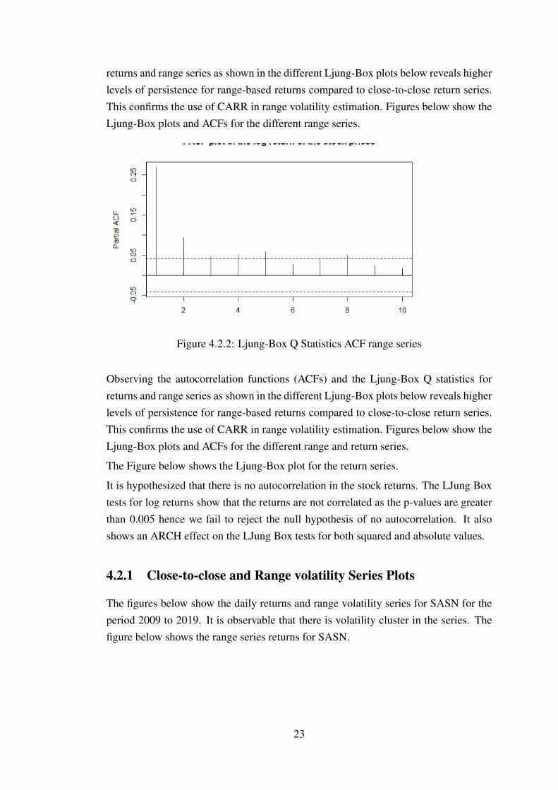
returns and range series as shown in the different Ljung-Box plots below reveals higherlevels of persistence for range-based returns compared to close-to-close return series.This confirms the use of CARR in range volatility estimation. Figures below show theLjung-Box plots and ACFs for the different range series.

Figure 4.2.2: Ljung-Box Q Statistics ACF range series

Observing the autocorrelation functions (ACFs) and the Ljung-Box Q statistics forreturns and range series as shown in the different Ljung-Box plots below reveals higherlevels of persistence for range-based returns compared to close-to-close return series.This confirms the use of CARR in range volatility estimation. Figures below show theLjung-Box plots and ACFs for the different range and return series.

The Figure below shows the Ljung-Box plot for the return series.

It is hypothesized that there is no autocorrelation in the stock returns. The LJung Boxtests for log returns show that the returns are not correlated as the p-values are greaterthan 0.005 hence we fail to reject the null hypothesis of no autocorrelation. It alsoshows an ARCH effect on the LJung Box tests for both squared and absolute values.

4.2.1 Close-to-close and Range volatility Series Plots

The figures below show the daily returns and range volatility series for SASN for theperiod 2009 to 2019. It is observable that there is volatility cluster in the series. Thefigure below shows the range series returns for SASN.

23

Figure 4.2.3: SASN Range Series Returns

Figure 4.2.4: SASN Daily Series Returns

The figure below shows the close-to-close volatility series for SASN.

24

Figure 4.2.5: SASN Close-to-Close Volatility Series Returns

The figure below shows the Garman Klass Volatility series for SASN

Figure 4.2.6: SASN Garman Klass Volatility Series

All the series return plots show clustering.

4.2.2 GARCH-type Modeling

In GARCH and TARCH modeling, the number of lags are p and q, while CARR hasthree lags, p, q, and s. The Range GARCH and Range TARCH models also have p,q, and s. The model estimates were carried out with the consideration of p = q =

s = 1 thus obtaining improved accuracy and fewer number of parameters. We can test

25

Parameter RGARCH GARCH CARR (1,1) TARCH(1,1) RTARCH(1,1)ω -0.00018 0.00023 0.00039 -0.000221 0.00083α 0.163041 0.239382 0.57226 -0.53658 0.17597β 0.62931 0.584423 0.48479 0.52402 0.73334γ 0.02905 0.12321θ 0.002 - - - 0.0016

LogLikelihood 5760.99 5396.59 5497.209 5545.72 5814.203AIC -4.2964 -4.0243 -4.0980 -4.1342 -4.3346BIC -4.2832 -4.0111 -4.0804 -4.1166 -4.3282

Table 4.2: The Table details return and range-based volatility model estimates forSASINI, 2009-2019

the different models for validity based on the parameter estimates. For TARCH andRTARCH models, they had an α +γ greater than zero and p−value = 0.05 for testingstatistical significance. γ is greater than 0 hence show of leverage effect. α + β isgreater than 0 hence volatility persistence which can be confirmed from the return andrange-series plots.

The Table 4.2 shows the estimates for return and range-based volatility models forSASN. The ω value in each model is significant hence appropriate to conclude that themodels are affected by news.

From the parameter estimates in Table 4.2, it is only the asymmetric models TARCHand RTARCH which do not exhibit effect of past squared returns from the α . It is neg-atively related to volatility while in the symmetric models GARCH, RGARCH, andCARR α is positive indicative positive relation to volatility. The value of β for theRange CARR model is the lowest compared to the other models. This indicates shortterm memory in its volatility process compared to the other models. RTARCH hasthe longest memory in its volatility process. In the models, γ measures the leverageeffect. A value of γ that is greater than 0 indicates that leverage effect exists while aγ value not equal to zero indicates asymmetry Maciel and Ballini [2017]. Leverageeffects means that the volatility of the assets respond to negative and positive returns.The Θ parameter in the RTARCH and RGARCH models show that the models providemore information to volatility modeling for SASN stock than the other models. Thisanswers the research hypothesis whether range provides more information to volatil-ity modeling than using historical approach. Akaike Information Criterion (AIC) andBayesian Information Criterion are used to assess simplicity of the models Degian-nakis and Livada [2013]. Lower AIC and BIC values indicate that the model is thebest-performing volatility compared to the others based on the two criteria. In theanalysis from the table results, RTARCH model had the lowest AIC and BIC, and thenRGARCH model.

26

Models MSE QLIKECARR(1,1) 0.000103 -7.5378

RTARCH (1,1,1) 0.0009398 -7.00708RGARCH(1,1,1) 0.0009496 -7.0218

TARCH (1,1) 0.0009704 -GARCH (1,1) 0.000917398 -6.69765

Table 4.3: At 5 % significance level. MSE & QLIKE assessment for volatility fore-casting, ranked from best-performing to least

4.3 MSE and QLIKE Loss Functions

The performance of the volatility models is assessed using MSE and QLIKE loss func-tion. Realized volatility calculated using 1-day quotations of SASN data was used inwhich the period 2009 to 2014 was take as the out-of-sample volatility forecasting. Thelast observation was removed to ensure all observations are of the same size. MSE andQLIKE loss functions for the 4 models was computers. Lower MSE and QLIKE val-ues indicate higher performance of the model. From the analysis, range-based models,RGARCH, CARR, and RTARCH provided lower QLIKE and MSE values comparedto their counterparts in which close-to-close returns approach was followed, GARCHand TARCCH models. This observation was expected because standard GARCH-typemodels have limited information which includes only the daily returns. TARCH modelhad the highest loss function values while CARR outperformed RGARCH based onMSE and QLIKE criteria. TARCH and RTACH models was best-performing volatil-ity forecast compared to GARCH and RGARCH. However, RGARCH and RTARCHmodels provided crucial information to the process of volatility because they per-formed better in forecasts than GARCH and TARCH. Based on QLIKE and MSEvalues, CARR model gave the best results, that is low loss function values.

From the analysis, CARR model was the best-performing in overall because it had thelowest MSE and QLIKE Loss functions. RGARCH, RTARCH and CARR performedbetter than TARCH and GARCH as seen by the MSE and QLIKE valuess.

4.4 Diebold-Mariano Test

Diebold-Mariano test was conducted to assess the equivalence of accuracy of the dif-ferent model pairs. The DM tests are statistically significant at 5% for CARR Modelwhen compared with the critical value of 1.96. α = 0.05 is divided by two because thetest is two sided hence the upper is 0.975. Based on DM test, CARR model outper-forms GARCH model. The improved performance of CARR model may be attributedto the fact that it uses range instead of return-based volatility like GARCH models.

27

Models TARCH RGARCH RTARCH CARRGARCH 0.42802 -6.8313 -6.5644 -6.9087TARCH - - -6.7111 -6.9879

RGARCH - - -3.9096 -8.3576RTARCH - - - -8.0802

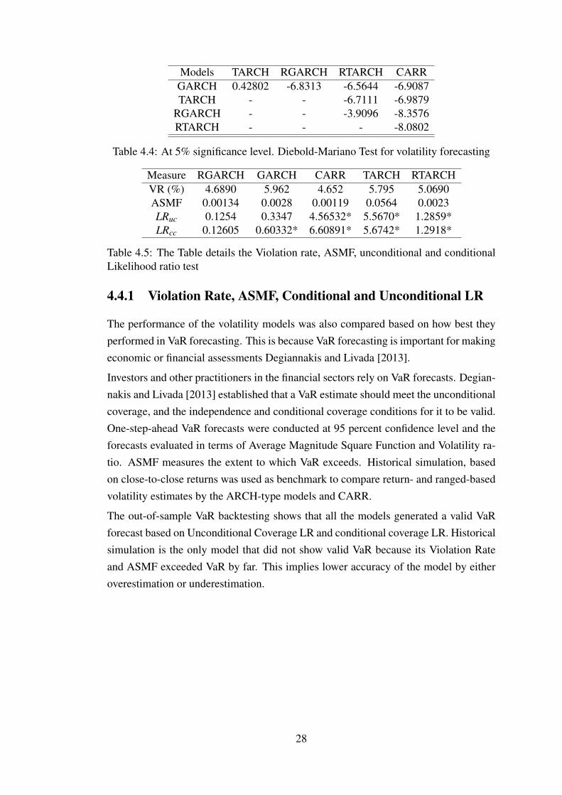
Table 4.4: At 5% significance level. Diebold-Mariano Test for volatility forecasting

Measure RGARCH GARCH CARR TARCH RTARCHVR (%) 4.6890 5.962 4.652 5.795 5.0690ASMF 0.00134 0.0028 0.00119 0.0564 0.0023LRuc 0.1254 0.3347 4.56532* 5.5670* 1.2859*LRcc 0.12605 0.60332* 6.60891* 5.6742* 1.2918*

Table 4.5: The Table details the Violation rate, ASMF, unconditional and conditionalLikelihood ratio test

4.4.1 Violation Rate, ASMF, Conditional and Unconditional LR

The performance of the volatility models was also compared based on how best theyperformed in VaR forecasting. This is because VaR forecasting is important for makingeconomic or financial assessments Degiannakis and Livada [2013].

Investors and other practitioners in the financial sectors rely on VaR forecasts. Degian-nakis and Livada [2013] established that a VaR estimate should meet the unconditionalcoverage, and the independence and conditional coverage conditions for it to be valid.One-step-ahead VaR forecasts were conducted at 95 percent confidence level and theforecasts evaluated in terms of Average Magnitude Square Function and Volatility ra-tio. ASMF measures the extent to which VaR exceeds. Historical simulation, basedon close-to-close returns was used as benchmark to compare return- and ranged-basedvolatility estimates by the ARCH-type models and CARR.

The out-of-sample VaR backtesting shows that all the models generated a valid VaRforecast based on Unconditional Coverage LR and conditional coverage LR. Historicalsimulation is the only model that did not show valid VaR because its Violation Rateand ASMF exceeded VaR by far. This implies lower accuracy of the model by eitheroverestimation or underestimation.

28

Figure 4.4.1: Actual & Forecasted Volatility Plot, RGARCH Model

The 1-step-ahead volatility forecast using RGARCH shows that the volatility forecastswere slightly lower than the actual.

Figure 4.4.2: RGARCH Model fitting plots. Different gaphs we obtained for 4-yearsahead forecasts

The plots for testing for normalitty, autocorrelation ACF, news impact curve,and skew-ness.

The graph below shows the volatility forecasts fore the competing models.

Range-based volatility models such as had lower violation rates and ASMF loss func-tion values. According to the coverage tests, CARR has significantly lower failurerate. This implies that the model overestimated VaR values. The practical implication

29

Figure 4.4.3: Comparison of 1-step-ahead volatility forecasts for the competing models

Figure 4.4.4: CARR Model, 1-step-ahead forecasts

of this results is that the risk-averse investors may end up taking unnecessary position.RTARCH and RGARCH more accurately estimated VaR at the 5% expected failurerate. These models also exhibit improved VaR forecasts hence higher accuracy com-pared to GARCH and TARCH models. We can conclude that range provided additionalinformation which improved the models.

The plot below shows the VaR forecasts for CARR Model

The plot below shows the VaR forecasts with RGARCH Model

4.5 Interpretation of Results

The Range-based CARR model proved to be the most efficient volatility in general.Also, RGARCH model performed better than the other GARCH-type and TARCH

30

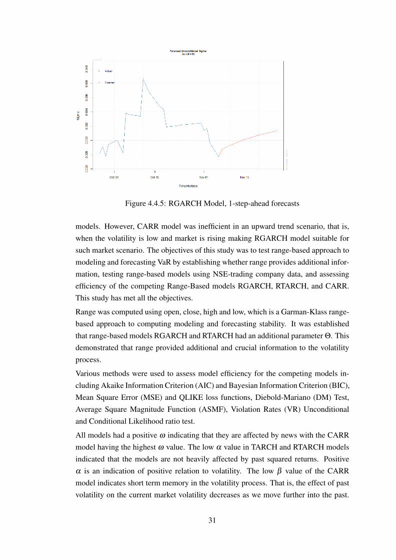
Figure 4.4.5: RGARCH Model, 1-step-ahead forecasts

models. However, CARR model was inefficient in an upward trend scenario, that is,when the volatility is low and market is rising making RGARCH model suitable forsuch market scenario. The objectives of this study was to test range-based approach tomodeling and forecasting VaR by establishing whether range provides additional infor-mation, testing range-based models using NSE-trading company data, and assessingefficiency of the competing Range-Based models RGARCH, RTARCH, and CARR.This study has met all the objectives.

Range was computed using open, close, high and low, which is a Garman-Klass range-based approach to computing modeling and forecasting stability. It was establishedthat range-based models RGARCH and RTARCH had an additional parameter Θ. Thisdemonstrated that range provided additional and crucial information to the volatilityprocess.

Various methods were used to assess model efficiency for the competing models in-cluding Akaike Information Criterion (AIC) and Bayesian Information Criterion (BIC),Mean Square Error (MSE) and QLIKE loss functions, Diebold-Mariano (DM) Test,Average Square Magnitude Function (ASMF), Violation Rates (VR) Unconditionaland Conditional Likelihood ratio test.

All models had a positive ω indicating that they are affected by news with the CARRmodel having the highest ω value. The low α value in TARCH and RTARCH modelsindicated that the models are not heavily affected by past squared returns. Positiveα is an indication of positive relation to volatility. The low β value of the CARRmodel indicates short term memory in the volatility process. That is, the effect of pastvolatility on the current market volatility decreases as we move further into the past.

31

Volatility a hundred days ago has lesser influence on today’s volatility than volatilityfrom 50 or lesser time period.

Minimum AIC and BIC values are used as selection criteria. Models with high log-likelihood have low AIC values hence superior goodness-of-fit. AIC assesses themodel that adequately describes an unknown while BIC is used to find the true modelamong the competing volatility models.

QLIKE and MSE are selected because they are robust loss functions, hence less af-fected by the most extreme observations in the sample. MSE loss function relies onthe usual forecast error (σ)2−h. Lower MSE and QLIKE values imply a better model.From Table 4.3, the MSE and QLIKE loss values were obtained at 5 percent confidencelevel. It was observed that CARR model had the lowest MSE and QLIKE values fol-lowed by RTARCH and RGARCH models with GARCH model performing least.

The DM test assess equivalence of accuracy among competing models. At 5 percentlevel of significance, CARR model was observed to have the lowest DM statistic valuescompared with corresponding model pairs. Violation rates, ASMF and Conditional andunconditional likelihood ratio tests were carried out on the competing models based onthe one-step-ahead VaR forecasts. Range-based volatility models had lower violationand ASMF values indicating lower failure r ates hence better performance. ASMFmeasures VaR exceedance, that is how far the forecasts exceeded realized VaR. At95 percent confidence level, range-based models perform better than close-to-closereturn-based models. CARR model outperforms the other RGARCH models based onmost of the measures for selecting suitable model.

32

Chapter 5

Conclusions and Recommendations

5.1 Conclusions

Based on the various model valuation criteria, the criteria indicate that forecasting errorof CARR (1,1) is low than that of GARCH (1,1). The conclusion is that CARR modeloutperforms the GARCH model. The range-based models, RGARCH, RTARCH, andCARR support Chou [2005] proposition that the range provides more information thanreturn. CARR (1,1) provides a sharper volatility forecasts than range-based GARCHand TARCH models.

The goal of this study was to provide a simple and highly effective approach for fore-casting the volatility of returns by using range rather than the daily returns. It wasthe study’s objective to determine the research hypothesis whether range and the pricemovements during the day affect the returns and hence use of range-based volatilityapproach to model and forecast volatility. Also, the aim was to establish applicabilityof the method by conducting empirical analysis of an NSE-listed and trading company,SASN.

On empirical analysis, it was established that using information contained in range sig-nificantly improves the accuracy of the volatility estimates. GARCH model performsbetter than CARR model when the volatilities are lower and the market is rising basedon symmetric and asymmetric error statistics. Therefore, in downward trend, volatilityis higher and the CARR model is more appropriate hence preferable.

However, in upward trend, it is crucial to use all daily information. That is, open, high,low, and close to determine and efficient volatility measure because using only openingand closing prices may wrongly conclude the volatility estimate. We can conclude thatrange-based volatility estimates provide additional information to forecasting volatilityhence more accurate than return-based volatility estimates.

33

5.2 Recommendations

5.3 Room for Further Research

The results are not highly optimized and stand for purposes of comparison. Achiev-ing higher accuracy could require large input data. Future research should explore thedegree of accuracy to which the volatility estimates can be forecasted with large datainput. We only used the daily price range data to make forecasts of a day ahead and thishas its shortcomings which include the small data set used for making relatively longperiod forecasts. It would be worth to explore the predictability of realized volatili-ties obtained from intraday data. This study recommends further research to includelong-term forecasting models, address volatility patterns such as crisis scenarios andapplication to trading strategies.

34

References

Ozgur Ozzy Akay, Mark D. Griffiths, and Drew B. Winters. On the robustness ofrange-based volatility estimators. Journal of Financial Research, 2010.

Torben G. Andersen, Tim Bollerslev, Francis X. Diebold, and Paul Labys. Modelingand forecasting realized volatility. Econometrica, 71:579–625, 03 2003. doi: 10.1111/1468-0262.00418.

Randy I. Anderson, Yi-Chi Chen, and Li-Min Wang. A range-based volatility approachto measuring volatility contagion in securitized real estate markets. Economic Mod-

elling, 45:223–235, 02 2015. doi: 10.1016/j.econmod.2014.10.058.

Noureddine Benlagha and Sana Chargui. Range-based and garch volatility estimation:Evidence from the french asset market. Global Finance Journal, 32:149–165, 022017. doi: 10.1016/j.gfj.2016.04.001.

Benjamin M. Blau and Ryan J. Whitby. Range-based volatility, expected stock returns,and the low volatility anomaly. PLOS ONE, 12, 11 2017. doi: 10.1371/journal.pone.0188517.

Michael W Brandt and Christopher S Jones. Volatility forecasting with range-basedegarch models. Journal of Business and Economic Statistics, 2002.

Michael W Brandt and Christopher S Jones. Volatility forecasting with range-basedegarch models. Journal of Business & Economic Statistics, 24:470–486, 10 2006.doi: 10.1198/073500106000000206.

Heng-Chih Chou and David K. Wang. Estimation of tail-related value-at-risk mea-sures: Range-based extreme value approach. Quantitative Finance, 14:293–304, 092014. doi: 10.1080/14697688.2013.819113.

Ray Yeu-Tien Chou. Forecasting financial volatilities with extreme values: The con-ditional autoregressive range (carr) model. Journal of Money, Credit, and Banking,37:561–582, 2005. doi: 10.1353/mcb.2005.0027.

35

Ray Yeutien Chou and Nathan Liu. The economic value of volatility timing usinga range-based volatility model. Journal of Economic Dynamics and Control, 34:2288–2301, 11 2010. doi: 10.1016/j.jedc.2010.05.010.

Ray Yeutien Chou, Chun-Chou Wu, and Nathan Liu. Forecasting time-varyingcovariance with a range-based dynamic conditional correlation model. Review

of Quantitative Finance and Accounting, 33:327–345, 03 2009. doi: 10.1007/s11156-009-0113-3.

Ray Yeutien Chou, Hengchih Chou, and Nathan Liu. Range volatility: A review ofmodels and empirical studies. Handbook of Financial Econometrics and Statistics,pages 2029–2050, 08 2014. doi: 10.1007/978-1-4614-7750-1_74.

Stavros Degiannakis and Alexandra Livada. Realized volatility or price range: Evi-dence from a discrete simulation of the continuous time diffusion process. Economic

Modelling, 30:212–216, 01 2013. doi: 10.1016/j.econmod.2012.09.027.

Francis X. Diebold and Roberto S. Mariano. Comparing predictive accuracy. Journal

of Business & Economic Statistics, 13:253–263, 07 1995. doi: 10.1080/07350015.1995.10524599.

Robert Engle. New frontiers for arch models. Journal of Applied Econometrics, 17(5):425–446, 2002.

Mark B. Garman and Michael J. Klass. On the estimation of security price volatilitiesfrom historical data. The Journal of Business, 53:67, 01 1980. doi: 10.1086/296072.

Robert Gathaiya. Analysis of issues affecting collapsed banks in kenya from year 2015to 2016. International Journal of Management and Business Studies, 2017.

Lawrence R Glosten, Ravi Jagannathan, and David E Runkle. On the relation betweenthe expected value and the volatility of the nominal excess return on stocks. The

journal of finance, 48(5):1779–1801, 1993.

Paul Kupiec. Techniques for verifying the accuracy of risk measurement models. The

J. of Derivatives, 3(2), 1995.

Hongquan Li and Yongmiao Hong. Financial volatility forecasting with range-basedautoregressive volatility model. Finance Research Letters, 8:69–76, 06 2011. doi:10.1016/j.frl.2010.12.002.

Leandro dos Santos Maciel and Rosangela Ballini. Value-at-risk modeling and fore-casting with range-based volatility models: empirical evidence. Revista Contabili-

dade & Finanças, 28:361–376, 12 2017. doi: 10.1590/1808-057x201704140.

36

Michael Parkinson. The extreme value method for estimating the variance of the rateof return. The Journal of Business, 53:61, 01 1980. doi: 10.1086/296071. URLhttps://www.cmegroup.com/trading/fx/files/michael_parkinson.pdf.

Andrew J. Patton. Volatility forecast comparison using imperfect volatility proxies.Journal of Econometrics, 160:246–256, 01 2011. doi: 10.1016/j.jeconom.2010.03.034.

Gábor Petneházi and József Gáll. Exploring the predictability of range-based volatil-ity estimators using recurrent neural networks. Intelligent Systems in Accounting,

Finance and Management, 26(3):109–116, 2019.

Ronald D. Ripple and Imad A. Moosa. The effect of maturity, trading volume, and openinterest on crude oil futures price range-based volatility. Global Finance Journal,20:209–219, 2009. doi: 10.1016/j.gfj.2009.06.001.

Prateek Sharma et al. Forecasting stock market volatility using realized garch model:International evidence. The Quarterly Review of Economics and Finance, 59:222–230, 2016.

Jinghong Shu and Jin E. Zhang. Testing range estimators of historical volatility. Jour-

nal of Futures Markets, 26:297–313, 2006. doi: 10.1002/fut.20197.

37

38

R Notebook

library(quantmod)

## Loading required package: xts

## Loading required package: zoo

#### Attaching package: 'zoo'

## The following objects are masked from 'package:base':#### as.Date, as.Date.numeric

## Loading required package: TTR

## Registered S3 method overwritten by 'quantmod':## method from## as.zoo.data.frame zoo

## Version 0.4-0 included new data defaults. See ?getSymbols.library(xts)library(rvest)

## Loading required package: xml2library(tidyverse)

## v ggplot2 3.3.2 v purrr 0.3.4## v tibble 3.0.3 v dplyr 1.0.0## v tidyr 1.1.0 v stringr 1.4.0## v readr 1.3.1 v forcats 0.5.0

library(stringr)library(forcats)library(lubridate)

#### Attaching package: 'lubridate'

## The following objects are masked from 'package:base':#### date, intersect, setdiff, union

1

## -- Conflicts ---------------------------------------------------## x dplyr::filter() masks stats::filter()## x dplyr::first() masks xts::first()## x readr::guess_encoding() masks rvest::guess_encoding()## x dplyr::lag() masks stats::lag()## x dplyr::last() masks xts::last()## x purrr::pluck() masks rvest::pluck()

library(plotly)

#### Attaching package: 'plotly'

## The following object is masked from 'package:ggplot2':#### last_plot

## The following object is masked from 'package:stats':#### filter

## The following object is masked from 'package:graphics':#### layoutlibrary(dplyr)library(PerformanceAnalytics)

#### Attaching package: 'PerformanceAnalytics'

## The following object is masked from 'package:graphics':#### legendlibrary(quantmod)library(rugarch)

## Loading required package: parallel

#### Attaching package: 'rugarch'

## The following object is masked from 'package:purrr':#### reduce

## The following object is masked from 'package:stats':#### sigmalibrary(rmgarch)

#### Attaching package: 'rmgarch'

## The following objects are masked from 'package:dplyr':#### first, last

## The following objects are masked from 'package:xts':#### first, lastlibrary(ggfortify)library(changepoint)

2

#### Attaching package: 'changepoint'

## The following object is masked from 'package:rugarch':#### likelihoodlibrary(strucchange)

## Loading required package: sandwich

#### Attaching package: 'strucchange'

## The following object is masked from 'package:stringr':#### boundarylibrary(ggpmisc)library(ModelMetrics)

#### Attaching package: 'ModelMetrics'

## The following object is masked from 'package:base':#### kappalibrary(pastecs)

#### Attaching package: 'pastecs'

## The following objects are masked from 'package:rmgarch':#### first, last

## The following objects are masked from 'package:dplyr':#### first, last

## The following object is masked from 'package:tidyr':#### extract

## The following objects are masked from 'package:xts':#### first, lastlibrary(MCS)library(MatrixCorrelation)

#### Attaching package: 'MatrixCorrelation'

## The following object is masked from 'package:TTR':#### SMIlibrary(multDM)

3

#Upload Datasetwd("C:/Users/USER/Desktop/Resources Project")mydata <-read.csv("mydata1.csv")attach(mydata)#plot Range Returnsplot.ts(mydata$SASN.RANGE.Returns,ylab="Range-Based Returns")

Time

Ran

ge−

Bas

ed R

etur

ns

0 500 1000 1500 2000 2500

0.00

0.05

0.10

0.15

# plot close-close returnsplot.ts(SASN.Return.based,col="Blue", ylab="Daily Returns")

4

Time

Dai

ly R

etur

ns

0 500 1000 1500 2000 2500

−0.

2−

0.1

0.0

0.1

0.2

# plot Parkinson Volatilityplot.ts(mydata$Parkinson,col="Blue",ylab="Volatility")

5

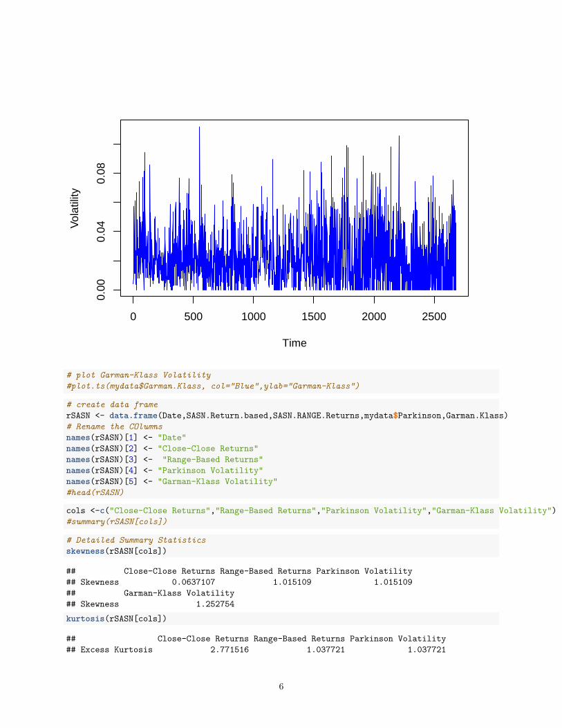
Time

Vol

atili

ty

0 500 1000 1500 2000 2500

0.00

0.04

0.08

# plot Garman-Klass Volatility#plot.ts(mydata$Garman.Klass, col="Blue",ylab="Garman-Klass")

# create data framerSASN <- data.frame(Date,SASN.Return.based,SASN.RANGE.Returns,mydata$Parkinson,Garman.Klass)# Rename the COlumnsnames(rSASN)[1] <- "Date"names(rSASN)[2] <- "Close-Close Returns"names(rSASN)[3] <- "Range-Based Returns"names(rSASN)[4] <- "Parkinson Volatility"names(rSASN)[5] <- "Garman-Klass Volatility"#head(rSASN)

cols <-c("Close-Close Returns","Range-Based Returns","Parkinson Volatility","Garman-Klass Volatility")#summary(rSASN[cols])

# Detailed Summary Statisticsskewness(rSASN[cols])

## Close-Close Returns Range-Based Returns Parkinson Volatility## Skewness 0.0637107 1.015109 1.015109## Garman-Klass Volatility## Skewness 1.252754kurtosis(rSASN[cols])

## Close-Close Returns Range-Based Returns Parkinson Volatility## Excess Kurtosis 2.771516 1.037721 1.037721

6

## Garman-Klass Volatility## Excess Kurtosis 1.73966# Descriptive Statistics#stat.desc(rSASN[cols], norm = "TRUE")

#Plot Time Series Returns and Volatility with date a-axisplot.ts(rSASN$`Close-Close Returns`,col="Blue",ylab="")

Time

0 500 1000 1500 2000 2500

−0.

2−

0.1

0.0

0.1

0.2

Box.test(rSASN$`Close-Close Returns`, type="Ljung-Box")

#### Box-Ljung test#### data: rSASN$`Close-Close Returns`## X-squared = 123.21, df = 1, p-value < 2.2e-16acf(rSASN$`Close-Close Returns`)

7

0 5 10 15 20 25 30 35

−0.

20.

20.

40.

60.

81.

0

Lag

AC

FSeries rSASN$`Close−Close Returns`

Box.test(rSASN$`Range-Based Returns`, type="Ljung-Box")

#### Box-Ljung test#### data: rSASN$`Range-Based Returns`## X-squared = 286.43, df = 1, p-value < 2.2e-16acf(rSASN$`Range-Based Returns`)

8

0 5 10 15 20 25 30 35

0.0

0.2

0.4

0.6

0.8

1.0

Lag

AC

FSeries rSASN$`Range−Based Returns`

Box.test(rSASN$`Parkinson Volatility`, type="Ljung-Box")

#### Box-Ljung test#### data: rSASN$`Parkinson Volatility`## X-squared = 286.43, df = 1, p-value < 2.2e-16acf(rSASN$`Parkinson Volatility`)

9

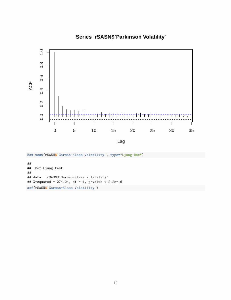
0 5 10 15 20 25 30 35

0.0

0.2

0.4

0.6

0.8

1.0

Lag

AC

FSeries rSASN$`Parkinson Volatility`

Box.test(rSASN$`Garman-Klass Volatility`, type="Ljung-Box")

#### Box-Ljung test#### data: rSASN$`Garman-Klass Volatility`## X-squared = 274.04, df = 1, p-value < 2.2e-16acf(rSASN$`Garman-Klass Volatility`)

10

0 5 10 15 20 25 30 35

0.0

0.2

0.4

0.6

0.8

1.0

Lag

AC

FSeries rSASN$`Garman−Klass Volatility`

# Assign model to standard specification, Range GARCH(1,1)ug_spec = ugarchspec()# GARCH Estimation using SASN datasasn_ugfit = ugarchfit(spec = ug_spec, data = SASN.RANGE.Returns)#sasn_ugfit

plot(sasn_ugfit, which = "all")

#### please wait...calculating quantiles...

11

1970 1974

0.00

Series with 2 Conditional SD Superimposed

Time

Ret

urns

GA

RC

H m

odel

: s

GA

RC

H

1970 1974

0.00

Series with with 1% VaR Limits

Time

Ret

urns

GA

RC

H m

odel

: sG

AR

CH

1970 1974

0.00

Conditional SD (vs |returns|)

Time

Vol

atili

ty

GA

RC

H m

odel

: s

GA

RC

H

1 8 17 27

ACF of Observations

lag

AC

F

0.0 GA

RC

H m

odel

: s

GA

RC

H

1 8 17 27

ACF of Squared Observations

lag

AC

F

0.0 GA

RC

H m

odel

: s

GA

RC

H

1 8 17 27

ACF of Absolute Observations

lag

AC

F

0.0 GA

RC

H m

odel

: s

GA

RC

H

−34 −9 9 27

Cross−Correlations of Squared vs Actual Observations

lag

AC

F

0.0

1.0

GA

RC

H m

odel

: s

GA

RC

H

Empirical Density of Standardized Residuals

zseries

Pro

babi

lity

−2 2 4 6

0.0

0.6 Median: −0.14 | Mean: 0.017

GA

RC

H m

odel

: s

GA

RC

H

normal Densitynorm (0,1) Fitted Density

−3 0 2

−2

4

norm − QQ Plot

Theoretical Quantiles

Sam

ple

Qua

ntile

s

GA

RC

H m

odel

: s

GA

RC

H

1 8 17 27

ACF of Standardized Residuals

lag

AC

F

−0.

04 GA

RC

H m

odel

: s

GA

RC

H

1 8 17 27

ACF of Squared Standardized Residuals

lag

AC

F

−0.

04 GA

RC

H m

odel

: s

GA

RC

H

−0.06 0.00 0.06

0.00

07

News Impact Curve

εt−1

σ t2

GA

RC

H m

odel

: s

GA

RC

H

# Check Elementspaste("Elements in the @model slot")

## [1] "Elements in the @model slot"#names(sasn_ugfit@model)#names(sasn_ugfit@fit)

# Extract estimated coefficients#sasn_ugfit@fit$coef

sasn_var <- sasn_ugfit@fit$var # Assign estimated conditional variancessasn_res2 <- (sasn_ugfit@fit$residuals)^2 # assign the estimated squared residuals#plot squared residuals and conditional varianceplot(sasn_res2, type = "l",col="Red",xlab="Index", ylab ="Residuals & Variance")lines(sasn_var, col = "blue")

12

0 500 1000 1500 2000 2500

0.00

00.

010

0.02

0

Index

Res

idua

ls &

Var

ianc

e

# Forecast conditional volatility or square root of conditional variance, for 2678sasn_predict <- ugarchforecast(sasn_ugfit, n.ahead = 100)#sasn_predict

Sasn_spredict <- sasn_predict@forecast$sigmaFor#plot(Sasn_spredict, type = "l",main = "1-step-ahead Volatility Forecast",ylab="Volatility Forecast")

# plot sigma squaredsasn_pred1<-ts(sasn_ugfit@fit$sigma^2)#plot.ts(sasn_pred1,col="Blue",ylab="Variance")

ug_spec = ugarchspec()# GARCH Estimation using SASN data, Historicalsasn_ugfit_h <- ugarchfit(spec = ug_spec, data = SASN.Return.based)# plot fitted valuessasn_predf<-sasn_ugfit@fit$fitted.values#plot.ts(sasn_predf, col="Blue",ylab="")

# Plot the fprrecasts with the last 100 observations in the estimation.# Last 100 observations in variancesasn_var1 <- c(tail(sasn_var,100),rep(NA,10))# Get last 100 observations of residual valuessasn_res2t <- c(tail(sasn_res2,100),rep(NA,10))# Assign predicted valuesSasn_spredict <- c(rep(NA,100),(Sasn_spredict)^2)# Display the observationsplot(sasn_res2t, type = "l",ylab="Volatility")

13

lines(Sasn_spredict, col = "Red")# 100 days, 1-step-ahead volatilitylines(sasn_var1, col = "green")legend("topleft", legend=c("Observed","Forecast"), col=c("Green","Black"),lty=1:2,cex = 0.8)

0 20 40 60 80 100

0.00

00.

002

0.00

4

Index

Vol

atili

ty

ObservedForecast

Determining MSE and QLIKE for GARCH Model Abovesasn_range.retuns <-SASN.RANGE.Returns#str(sasn_range.retuns)sasn_range.predict<-ugarchboot(sasn_ugfit, n.ahead = 2679,method=c("Partial","Full")[1])#str(sasn_range.predict)#str(sasn_range.retuns)r.mse<-mse(rSASN$`Range-Based Returns`,sasn_ugfit@fit$sigma)#mse(rSASN$`Range-Based Returns`,ugfit@fit$sigma)# install.packages("MCS")r.qlike<- LossVol(rSASN$`Range-Based Returns`,sasn_ugfit@fit$sigma,which="QLIKE")r_qlike<-r.qlike[1]# length(Garman.Klass)# length(ugfit@fit$sigma)Loss.Functions<-data.frame(r.mse,r_qlike)names(Loss.Functions)[1] <- "MSE"names(Loss.Functions)[2] <- "QLIKE"#Loss.Functions

# computing Ratio Volatilityrgarch.RV<-RV( sasn_ugfit@fit$fitted.values,sasn_ugfit@fit$sigma)#rgarch.RV

14

ESTIMATING USING GARCH with Historical Return# Assign model to standard specification, GARCH(1,1)ug_spec = ugarchspec()# GARCH Estimation using SASN data, Historicalsasn_ugfit_h <- ugarchfit(spec = ug_spec, data = SASN.Return.based)#sasn_ugfit_h

#for the sasn_ugfit_h Model that uses historical returnssasn_var.h <- sasn_ugfit_h@fit$var # Assign estimated conditional variancessasn_res2.h <- (sasn_ugfit_h@fit$residuals)^2 # assign the estimated squared residuals#plot squared residuals and conditional varianceplot(sasn_res2.h, type = "l",col="Red",xlab="Index", ylab ="Residuals & Variance")lines(sasn_var.h, col = "blue")

0 500 1000 1500 2000 2500

0.00

0.02

0.04

0.06

Index

Res

idua

ls &

Var

ianc

e

USING GARCH(1,1,1) CARR ModelgarchMod_t <- ugarchspec(

variance.model=list(model="fGARCH",garchOrder=c(1,1),submodel="APARCH"),

mean.model=list(armaOrder=c(0,0),include.mean=TRUE,archm=TRUE,archpow=2),

distribution.model="std")

15

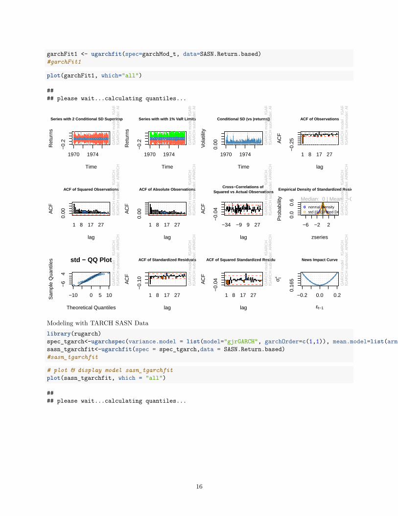
garchFit1 <- ugarchfit(spec=garchMod_t, data=SASN.Return.based)#garchFit1

plot(garchFit1, which="all")

#### please wait...calculating quantiles...

1970 1974

−0.

2

Series with 2 Conditional SD Superimposed

Time

Ret

urns

GA

RC

H m

odel

: fG

AR

CH

fGA

RC

H s

ubm

odel

: APA

RC

H

1970 1974

−0.

2

Series with with 1% VaR Limits

Time

Ret

urns

GA

RC

H m

odel

: fG

AR

CH

fGA

RC

H s

ubm

odel

: APA

RC

H

1970 1974

0.00

Conditional SD (vs |returns|)

Time

Vol

atili

ty

GA

RC

H m

odel

: fG

AR

CH

fGA

RC

H s

ubm

odel

: APA

RC

H

1 8 17 27

ACF of Observations

lag

AC

F

−0.

25 GA

RC

H m

odel

: fG

AR

CH

fGA

RC

H s

ubm

odel

: APA

RC

H

1 8 17 27

ACF of Squared Observations

lag

AC

F

0.00 GA

RC

H m

odel

: fG

AR

CH

fGA

RC

H s

ubm

odel

: APA

RC

H

1 8 17 27

ACF of Absolute Observations

lag

AC

F

0.00 GA

RC

H m

odel

: fG

AR

CH

fGA

RC

H s

ubm

odel

: APA

RC

H

−34 −9 9 27

Cross−Correlations of Squared vs Actual Observations

lag

AC

F

−0.

04 GA

RC

H m

odel

: fG

AR

CH

fGA

RC

H s

ubm

odel

: APA

RC

H

Empirical Density of Standardized Residuals

zseries

Pro

babi

lity

−6 −2 2

0.0

0.6 Median: 0 | Mean: −0.0175

GA

RC

H m

odel

: fG

AR

CH

fGA

RC

H s

ubm

odel

: APA

RC

H

normal Densitystd (0,1) Fitted Density

−10 0 5 10

−6

4

std − QQ Plot

Theoretical Quantiles

Sam

ple

Qua

ntile

s

GA

RC

H m

odel

: fG

AR

CH

fGA

RC

H s

ubm

odel

: APA

RC

H

1 8 17 27

ACF of Standardized Residuals

lag

AC

F

−0.

10

GA

RC

H m

odel

: fG

AR

CH

fGA

RC

H s

ubm

odel

: APA

RC

H

1 8 17 27

ACF of Squared Standardized Residuals

lag

AC

F

−0.

04 GA

RC

H m

odel

: fG

AR

CH

fGA

RC

H s

ubm

odel

: APA

RC

H

−0.2 0.0 0.20.

165

News Impact Curve

εt−1

σ t2

GA

RC

H m

odel

: fG

AR

CH

fGA

RC

H s

ubm

odel

: APA

RC

H

Modeling with TARCH SASN Datalibrary(rugarch)spec_tgarch<-ugarchspec(variance.model = list(model="gjrGARCH", garchOrder=c(1,1)), mean.model=list(armaOrder=c(2,0)),distribution.model="std")sasn_tgarchfit<-ugarchfit(spec = spec_tgarch,data = SASN.Return.based)#sasn_tgarchfit

# plot & display model sasn_tgarchfitplot(sasn_tgarchfit, which = "all")

#### please wait...calculating quantiles...

16

1970 1974

−0.

2Series with 2 Conditional SD Superimposed

Time

Ret

urns

GA

RC

H m

odel

: g

jrGA

RC

H

1970 1974

−0.

2

Series with with 1% VaR Limits

Time

Ret

urns

GA

RC

H m

odel

: gj

rGA

RC

H

1970 1974

0.00

Conditional SD (vs |returns|)

Time

Vol

atili

ty

GA

RC

H m

odel

: g

jrGA

RC

H

1 8 17 27

ACF of Observations

lag

AC

F

−0.

25 GA

RC

H m

odel

: g

jrGA

RC

H

1 8 17 27

ACF of Squared Observations

lag

AC

F

0.00 GA

RC

H m

odel

: g

jrGA

RC

H

1 8 17 27

ACF of Absolute Observations

lag

AC

F

0.00 GA

RC

H m

odel

: g

jrGA

RC

H

−34 −9 9 27

Cross−Correlations of Squared vs Actual Observations

lag

AC

F

−0.

04 GA

RC

H m

odel

: g

jrGA

RC

H

Empirical Density of Standardized Residuals

zseries

Pro

babi

lity

−8 −4 0 4

0.0

0.6 Median: 0 | Mean: −0.00599

GA

RC

H m

odel

: g

jrGA

RC

H

normal Densitystd (0,1) Fitted Density

−10 0 5 10

−8

2

std − QQ Plot

Theoretical Quantiles

Sam

ple

Qua

ntile

s

GA

RC

H m

odel

: g

jrGA

RC

H

1 8 17 27

ACF of Standardized Residuals

lag

AC

F

−0.

04

GA

RC

H m

odel

: g

jrGA

RC

H

1 8 17 27

ACF of Squared Standardized Residuals

lag

AC

F

−0.

04 GA

RC

H m

odel

: g

jrGA

RC

H

−0.2 0.0 0.2

0.12

0

News Impact Curve

εt−1

σ t2

GA

RC

H m

odel

: g

jrGA

RC

H

Modeling RTARCH# Using Range-basedsasn_tgarchfit.range<-ugarchfit(spec = spec_tgarch,data = SASN.RANGE.Returns)#sasn_tgarchfit.range

# plot RTARCH Range-based modelplot(sasn_tgarchfit.range,which="all")

#### please wait...calculating quantiles...

17

1970 1974

0.00

Series with 2 Conditional SD Superimposed

Time

Ret

urns

GA

RC

H m

odel

: g

jrGA

RC

H

1970 1974

0.00

Series with with 1% VaR Limits

Time

Ret

urns

GA

RC

H m

odel

: gj

rGA

RC

H

1970 1974

0.00

Conditional SD (vs |returns|)

Time

Vol

atili

ty

GA

RC

H m

odel

: g

jrGA

RC

H

1 8 17 27

ACF of Observations

lag

AC

F

0.0 GA

RC

H m

odel

: g

jrGA

RC

H

1 8 17 27

ACF of Squared Observations

lag

AC

F

0.0 GA

RC

H m

odel

: g

jrGA

RC

H

1 8 17 27

ACF of Absolute Observations

lag

AC

F

0.0 GA

RC

H m

odel

: g

jrGA

RC

H

−34 −9 9 27

Cross−Correlations of Squared vs Actual Observations

lag

AC

F

0.0

1.0

GA

RC

H m

odel

: g

jrGA

RC

H

Empirical Density of Standardized Residuals

zseries

Pro

babi

lity

−2 2 4 6

0.0

0.6 Median: −0.04 | Mean: 0.106

GA

RC

H m

odel

: g

jrGA

RC

H

normal Densitystd (0,1) Fitted Density

−4 0 4

−2

6

std − QQ Plot

Theoretical Quantiles

Sam

ple

Qua

ntile

s

GA

RC

H m

odel

: g

jrGA

RC

H

1 8 17 27

ACF of Standardized Residuals

lag

AC

F

−0.

04 GA

RC

H m

odel

: g

jrGA

RC

H

1 8 17 27

ACF of Squared Standardized Residuals

lag

AC

F

−0.

04 GA

RC

H m

odel

: g

jrGA

RC

H

−0.06 0.00 0.06

0.00

10

News Impact Curve

εt−1

σ t2

GA

RC

H m

odel

: g

jrGA

RC

H

tgarch.forecast<-sasn_tgarchfit.range@fit$residualstarch.forecast<-sasn_tgarchfit@fit$residualsrgarch.forecast<-sasn_ugfit@fit$residualsgarch.forecast<-sasn_ugfit_h@fit$residualscarr.forecast<-garchFit1@fit$residuals

# Computing Average Square Magnitude Function (ASMF)rgarch.ASMF<-sum(sasn_ugfit@fit$residuals)rgarch.ASMF

## [1] 2.048433#computing RV and ASMF for GARCH Modelgarch.RV<-RV(rSASN$`Range-Based Returns`,sasn_ugfit_h@fit$sigma)garch.ASMF<-sum(sasn_ugfit_h@fit$se.coef)

18

rgarch.mse<-mse(rSASN$`Range-Based Returns`,sasn_ugfit@fit$sigma)rgarch.qlike<- LossVol(rSASN$`Range-Based Returns`,sasn_ugfit@fit$sigma,which="QLIKE")garch.mse<-mse(rSASN$`Range-Based Returns`,sasn_ugfit_h@fit$sigma)garch.qlike<-LossVol(rSASN$`Range-Based Returns`,sasn_ugfit_h@fit$sigma,which="QLIKE")tarch.mse<-mse(rSASN$`Range-Based Returns`,sasn_tgarchfit@fit$sigma)tarch.qlike<-LossVol(rSASN$`Range-Based Returns`,sasn_tgarchfit@fit$sigma,which="QLIKE")rtarch.mse<-mse(rSASN$`Range-Based Returns`,sasn_tgarchfit.range@fit$sigma)rtarch.qlike<-LossVol(rSASN$`Range-Based Returns`,sasn_tgarchfit.range@fit$sigma,which="QLIKE")carr.mse<-mse(rSASN$`Range-Based Returns`,garchFit1@fit$sigma)carr.qlike<-LossVol(rSASN$`Range-Based Returns`,garchFit1@fit$sigma,which="QLIKE")#All.LossFunctions<-data.frame(rgarch.mse,rgarch.qlike,garch.mse,garch.qlike,tarch.mse,tarch.qlike,rtarch.mse,rtarch.qlike,carr.mse,carr.qlike)#All.LossFunctions

#garch.RV#garch.ASMF#computing RV and ASMF For CARR modelcarr.RV<-RV(rSASN$`Range-Based Returns`,garchFit1@fit$sigma)carr.ASMF<-sum(garchFit1@fit$se.coef)#carr.RV#carr.ASMF# computing RV and ASMF for TARCHtarch.Rv<-RV(rSASN$`Range-Based Returns`,sasn_tgarchfit@fit$sigma)tarch.ASMF<-sum(sasn_tgarchfit@fit$se.coef)#tarch.Rv#tarch.ASMF#computing RV and ASMF for RTARCHrtarch.RV <-RV(rSASN$`Range-Based Returns`,sasn_tgarchfit.range@fit$sigma)rtarch.ASMF <- sum(sasn_tgarchfit.range@fit$se.coef)#rtarch.RV#rtarch.ASMF

Determining Diebold-Mariano#install.packages("multDM")#GARCH vs TARCH#garch.tarch<-dm.test(garch.forecast,tarch.forecast,h=1)#garch.tarchDM.test(garch.forecast,tarch.forecast,rSASN$`Range-Based Returns`,loss.type = "SE",h=1)

#### Diebold-Mariano test#### data: garch.forecast and tarch.forecast and rSASN$`Range-Based Returns`## statistic = -6.6657, forecast horizon = 1, p-value = 2.634e-11## alternative hypothesis: Forecast f1 and f2 have different accuracy.

19

#GARCH vs RGARCHgarch.rgarch<-DM.test(garch.forecast,rgarch.forecast,rSASN$`Range-Based Returns`,loss.type = "SE",h=1)#garch.rgarch#GARCH vs RTARChgarch.rtarch<-DM.test(garch.forecast,tgarch.forecast,rSASN$`Range-Based Returns`,loss.type = "SE",h=1)#garch.rtarch#GARCH vs CARRgarch.carr <- DM.test(garch.forecast,carr.forecast,rSASN$`Range-Based Returns`,loss.type = "SE",h=1)#garch.carr#TARCH vs RGARCHtarch.rgarch <-DM.test(tarch.forecast,rgarch.forecast,rSASN$`Range-Based Returns`,loss.type = "SE",h=1)#tarch.rgarch#TARCH vs RTARCHtarch.rtarch<-DM.test(tarch.forecast,tgarch.forecast,rSASN$`Range-Based Returns`,loss.type = "SE",h=1)#tarch.rtarch#RGARCH vs RTARCHrgarch.rtarch<-DM.test(rgarch.forecast,tgarch.forecast,rSASN$`Range-Based Returns`,loss.type = "SE",h=1)#rgarch.rtarch#RGARCH vs CARRrgarch.carr<-DM.test(rgarch.forecast,carr.forecast,rSASN$`Range-Based Returns`,loss.type = "SE",h=1)#rgarch.carr#RTARCH vs CARRrtarch.carr<-DM.test(tgarch.forecast,carr.forecast,rSASN$`Range-Based Returns`,loss.type = "SE",h=1)#rtarch.carr

20

Appendices

R Codes

library(stringr)library(forcats)library(lubridate)

#### Attaching package: 'lubridate'

## The following objects are masked from 'package:base':#### date, intersect, setdiff, union

1

39

R Notebook