R&D White Paper

WHP 001

April 2001

The calibration of VHF/UHF field strength measuring equipment

J. Middleton

Research & Development

BRITISH BROADCASTING CORPORATION

© BBC 2001. All rights reserved.

BBC Research & Development White Paper 001

The calibration of VHF/UHF field strength measuring equipment

J. Middleton

Abstract

Field strength measurement equipment, from the antenna to the receiver, must be calibrated before it is used for field work and this document describes how it is done at BBC R&D. A similar document was produced many years ago but, whilst the principles remain the same, the application and presentation needed updating owing to changes in the equipment now used.

Key words: VHF/UHF field strength, calibration

© BBC 2001. All rights reserved. Except as provided below, no part of this document may be reproduced in any material form (including photocopying or storing it in any medium by electronic means) without the prior written permission of BBC Research & Development except in accordance with the provisions of the (UK) Copyright, Designs and Patents Act 1988.

The BBC grants permission to individuals and organisations to make copies of the entire document (including this copyright notice) for their own internal use. No copies of this document may be published, distributed or made available to third parties whether by paper, electronic or other means without the BBC's prior written permission. Where necessary, third parties should be directed to the relevant page on BBC's website at http://www.bbc.co.uk/rd/pubs/whp for a copy of this document.

White Papers are distributed freely on request.

Authorisation of the Head of Research is required for publication.

BBC Research & Development White Paper WHP 001

The Calibration of VHF/UHF Field Strength

Measuring Equipment

Spectrum Planning Group

J. Middleton Contents 1 Introduction 2 General principles 2.1 Field strength 2.2 The measuring receiver

2.3 The antenna factor 2.4 Generating a standard field

3 Calibration procedures 3.1 Receiver checks 3.2 Measurement of feeder loss

3.3 Field calibration 3.4 Quick inspections

4 Conclusions 5 References Appendix 1 Calculating the K Factor Appendix 2 The voltage induced in a half-wave dipole Appendix 3 Free space field strength Appendix 4 Antenna calibration – The Ground Reflection Method Appendix 5 Antenna calibration - The UHF Diffraction Screen Method

© BBC 2001. All rights reserved.

1

1. Introduction This document describes the principles and practical details for calibrating equipment used for making VHF and UHF field strength measurements. However, it must be stressed that a wider knowledge of radio wave propagation effects and the characteristics of the equipment used are important to ensure the validity of subsequent measurements. The theoretical bases of the methods used have been presented as simply as possible to ensure ease of application and will provide a guide to certain important aspects of propagation although, for comprehensive analyses, it will be necessary to refer to the more extensive works which are available [1], [2].

The object of calibrating measuring equipment is not only to ensure that the accuracy lies within acceptable limits but also to establish whether any incipient faults or deficiencies occur when the equipment is used under actual working conditions. Careful attention should therefore be given to both the results obtained and to the performance of the equipment used during the calibration process. 2. General principles

2.1 Field strength

The term “field strength” refers to the intensity of either the electric or magnetic field components of electromagnetic radiation. The field strength of a uniform electric field is defined, in the MKS system, as being the potential difference existing in space between two points, 1 metre apart in the direction of the electric component of the radiation. It can be measured by placing an antenna, of known length, parallel to the electric component and measuring the voltage developed across its terminals.

The value of this voltage depends upon the “effective length” of the antenna. At VHF and UHF, the resonant half-wave dipole is normally used as the standard of reference. Its effective length can be shown to be λ/π (see Appendix 2). Hence the voltage at the terminals of a half-wave dipole, when in an electric field of strength e volts/metre, is given by:

πλev =

where λ is the wavelength in metres. In practice, a half-wave dipole is rarely used for measuring the field strength of radio and television transmissions since it lacks good directional properties and therefore responds to indirect signals. At VHF a dipole and reflector may be used and at higher frequencies multi-element arrays are used but, whatever the antenna, it is normal practice to express its gain relative to a half-wave dipole (i.e. in dBd). It is usual to express field strength in decibels relative to 1 µV/m (i.e. in dBµV/m).

2.2 The measuring receiver

A field strength measuring receiver is essentially a tuneable voltmeter. It enables the level of the RF signal, generated by an antenna, to be measured when tuned to the frequency of that signal. This level may be displayed on the receiver’s meter or conveyed via a suitable data link to a computer. The normal units of measurement are dB relative to 1 µV (dBµV), and the input impedance of the receiver is usually 50Ω although receivers with 75Ω are

2

occasionally used. A conversion factor must be used relate the voltage indicated by the receiver to the field strength at the antenna.

2.3 The Antenna Factor

The voltage at the receiver is related to the field strength at the antenna by a number of clearly defined factors, collectively known as the “antenna factor” or “K factor”. The elements of this antenna factor are the effective antenna length (see Appendix 2), antenna gain, feeder loss, and impedance and unit conversion factors.

Thus Field Strength = Receiver Voltage + K.

As shown in Appendix 1, the K factor of an antenna system is given by:

32- f 0+G-L = K Log2 dB

where L is the feeder loss in dB, G is the antenna gain in dBd, f is the frequency in MHz and the characteristic impedance of the system is 50Ω. The K factor should also be determined experimentally in order to check the correct operation and accuracy of the measuring system. To do this it is necessary to provide a standard field of known intensity. The antenna can then be placed in this field and the reading on the receiver noted. The difference in dB between the value of the standard field strength and the receiver indication is the K factor.

2.4 Generating a standard field

In practice, the difficulty lies in knowing with sufficient accuracy the strength of the standard field since, at VHF and UHF, reflections from the ground and surrounding obstacles can affect the field strength at the receiving antenna in a complex manner. The accuracy and reliability with which a physical quantity can be determined increases with the simplicity of the method. Experimental conditions are therefore chosen so that relatively simple analyses, based on easily measured parameters, are valid.

The field strength produced by an antenna radiating in free space is inversely proportional to distance (see Appendix 3), due simply to the spread of energy with increasing distance. Although this condition cannot readily be achieved, the “free space” field concept is a convenient basis for further discussion.

Two methods are used for obtaining a standard field, the Ground Reflection method, which is more appropriate at VHF (Appendix 4) and the Diffraction Screen method, which is used at UHF (Appendix 5). This variation of methods is analogous to the conditions occurring in practice for broadcast reception where, at VHF, the field strength values obtained are often determined to a considerable degree by the presence of ground reflections. At UHF this factor is less quantifiable due to the presence of obstacles and surface roughness.

Whichever method is used the objective is the same, to determine by practical experiment the K factor of the antenna system. The result obtained is then compared with the theoretical value calculated as described in Section 2.3. There should be close agreement between them, i.e. the difference between the practical K factor, and the theoretical K factor should not be greater than 1 dB.

3

3. The Calibration Procedure 3.1 Receiver checks A field strength measuring receiver is designed to indicate the level of the RF voltage applied to its input when tuned to the frequency of that signal. Such receivers can be configured in many different ways and the user must be certain that the receiver is set up appropriately for the type of signal to be measured. For example, when measuring analogue television signals, the vision carrier is normally used. If using the Rohde & Schwarz ESVB receiver, the bandwidth should be set to 300 kHz and the level detector set to Peak. Table 1 shows the settings to be used for other types of signal. Other receiver makes will have similar features but may differ in the number of options available.

Table 1 Typical receiver settings

Signaltype

Rx bandwidth(kHz)

Detectortype

Analogue TV 300 PeakFM radio 120 AverageDigital radio 1500 RMS

If the receiver is software controlled, the setting up should occur automatically when the logging software is started. However, it is up to the user to make certain that the configuration is correct. The level measuring capability of the receiver should be checked using a signal generator whose output has been confirmed using a power meter. A signal at the appropriate frequency is fed to the receiver and the indicated level compared with that at the input. Account must be taken of the loss of the connecting feeder. The levels used should be comparable to those that will be encountered during field work. This will highlight any problems that may arise through overloading or being too close to the receiver noise floor. 3.2 Measurement of feeder loss The measuring antenna is connected to the receiver through a length of suitable feeder. The loss of this feeder at the measurement frequencies must be known since feeder loss is one of the components of the K factor (see Section 2.3). Similarly, if antenna switches or pre-amplifiers are used, their loss/gain must be included. Feeder loss is most easily measured by substitution using a signal generator and a power meter or measuring receiver. 3.3 Field calibration

If the feeder loss has been measured and the receiving antenna gain is known then the K factor can be calculated using the equation given in Section 2.3. However, the antenna gain may be different from the expected value through damage or corrosion so, in addition to calculating the theoretical K factor, it should also be determined by direct measurement. If this is within 1 dB of the theoretical value then it can be assumed that the measuring system is functioning satisfactorily.

4

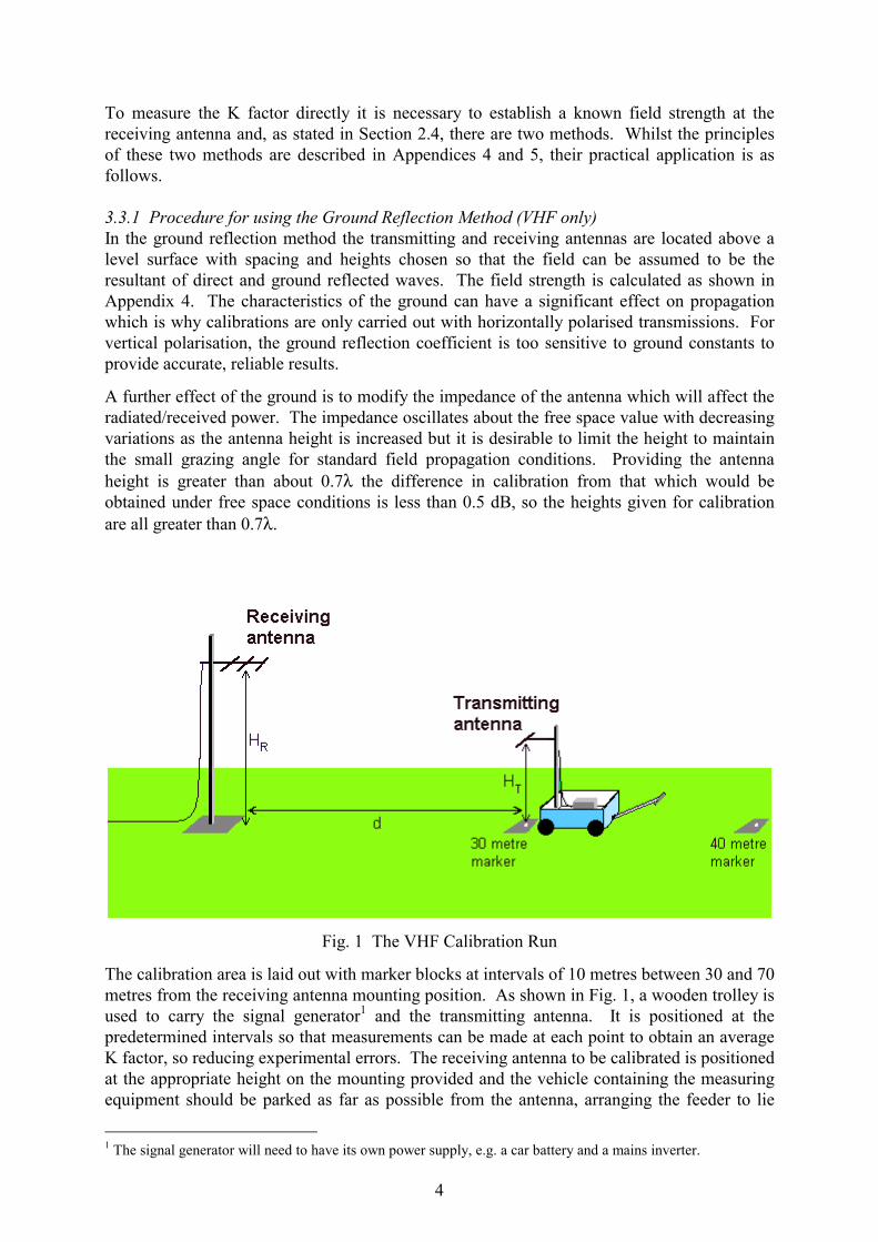
To measure the K factor directly it is necessary to establish a known field strength at the receiving antenna and, as stated in Section 2.4, there are two methods. Whilst the principles of these two methods are described in Appendices 4 and 5, their practical application is as follows. 3.3.1 Procedure for using the Ground Reflection Method (VHF only) In the ground reflection method the transmitting and receiving antennas are located above a level surface with spacing and heights chosen so that the field can be assumed to be the resultant of direct and ground reflected waves. The field strength is calculated as shown in Appendix 4. The characteristics of the ground can have a significant effect on propagation which is why calibrations are only carried out with horizontally polarised transmissions. For vertical polarisation, the ground reflection coefficient is too sensitive to ground constants to provide accurate, reliable results.

A further effect of the ground is to modify the impedance of the antenna which will affect the radiated/received power. The impedance oscillates about the free space value with decreasing variations as the antenna height is increased but it is desirable to limit the height to maintain the small grazing angle for standard field propagation conditions. Providing the antenna height is greater than about 0.7λ the difference in calibration from that which would be obtained under free space conditions is less than 0.5 dB, so the heights given for calibration are all greater than 0.7λ.

Fig. 1 The VHF Calibration Run

The calibration area is laid out with marker blocks at intervals of 10 metres between 30 and 70 metres from the receiving antenna mounting position. As shown in Fig. 1, a wooden trolley is used to carry the signal generator1 and the transmitting antenna. It is positioned at the predetermined intervals so that measurements can be made at each point to obtain an average K factor, so reducing experimental errors. The receiving antenna to be calibrated is positioned at the appropriate height on the mounting provided and the vehicle containing the measuring equipment should be parked as far as possible from the antenna, arranging the feeder to lie

1 The signal generator will need to have its own power supply, e.g. a car battery and a mains inverter.

5

behind the antenna as shown, to avoid distorting the field pattern. The signal generator should be switched on and allowed to stabilise and, before connecting the transmitter feeder, the required output power into a 50Ω load should be checked.

The transmitting trolley is then positioned at each point on the run and the receiver indication, VR noted at each position. The trolley should be positioned so that the active element of the antenna coincides with the appropriate ground marker as shown in Fig. 1. The voltage VR is subtracted from the theoretical field strength EH, calculated as shown in Appendix 4 for the appropriate heights and distance. The program 2rayCalc.exe facilitates this process.2 The K factor is then given by:

K = EH - VR

To minimise errors, the final K factor is obtained by averaging the individual values measured along the run. If this is within 1 dB of the theoretical K factor, calculated according to the equation given in Section 2.3, then the measuring setup under test has been validated.

With careful and systematic operating it should be possible to obtain the tolerance accuracy of ± l dB without undue difficulty. 3.3.2 Field calibration using the Diffraction Screen Method (UHF only)

The receiving antenna, mounted on the survey vehicle’s pneumatic mast, is located over the reference point associated with the diffraction screen as shown in Fig. 2. The system will work satisfactorily with either horizontal or vertical polarisation but the polarisation of the transmitting and receiving antennas must match. If necessary, the transmitting antenna can be rotated through 90° by operating a lever at the base of the tower.

Fig. 2 Layout of the diffraction screen facility

The signal generator is switched on and allowed to stabilise. Before connecting the transmitter feeder, the output power into a 50Ω load should be checked.

2 When using this program, the correct ERP must be entered, taking account of the gain of the transmitting antenna and the attenuation of the connecting feeder.

6

The hydraulic mast is then operated to raise the receiving antenna slowly. The receiver will indicate a steady rise in field strength up to a maximum value followed by a steady fall and the field strength will continue to oscillate in this way as the antenna rises to the limit of its travel. The distance between consecutive peaks varies with frequency, there being three full oscillations at 700 MHz as the antenna rises to 10 metres but only two at 500 MHz. Fig. 3 shows a typical field strength variation.

Fig. 3 Field strength variation at 756 MHz

The values of the second maximum and minimum are noted and the mean calculated. This mean value, VR is the receiver indication corresponding to the free space field strength, E0 obtained from Table A5.2 in Appendix 5. These field strength values assume a signal generator output of 0 dBm.

The practical K factor is then given by: K = Eo - VR

If this is within 1 dB of the theoretical K factor, calculated according to the equation given in Section 2.3, then the setup under test has been validated. 3.4 Quick inspections If a new antenna is being used for the first time, or if there is any doubt concerning an existing antenna system, a full calibration should always be carried out. In fact, ideally, antenna calibrations should be carried out prior to every survey. However the process is time consuming and it is not always realistic to do this. As an alternative, the performance of an antenna can be quickly assessed by connecting it to a network analyser. This will show if there are any frequency dependant mis-matches caused, for example, by corroded or damaged elements. The antenna should be mounted on a tripod, as shown in Fig. 4, pointing away from any adjacent structures, and connected with a short (3 metres) feeder.

7

Fig. 4 Testing the antenna using a network analyser

The network analyser should be set to display reflection coefficient. For the Chelton log-periodic antenna, if the reflection coefficient is well below 20% over the frequency range being used, then it can be safely assumed that the antenna performance will be as expected, i.e. the gain figures that were last used can still be considered valid. If the reflection coefficient goes above 20% then there is likely to be a problem. N.B. This measurement does not give gain information. Fig. 5a and Fig. 5b show reflection coefficient plots for valid and faulty antennas respectively. These were log-periodic antennas and, in the case of the faulty antenna, the problem was due to a loose element.

Fig. 5a Typical reflection coefficient plot Fig. 5b Typical reflection coefficient plot

for a for a valid antenna for a faulty antenna For other types of antenna, the minimum reflection coefficient may be different so the appropriate manufacturer’s specification should be consulted. Another point worth remembering for log-periodic antennas is that, over a period of time, corrosion can occur at the feed point. This is normally inaccessible and not easy to see but it can easily be checked by measuring the input resistance of the antenna. With no corrosion, the DC resistance should be zero.

4. Conclusions This document describes the principles and practice of calibrating VHF and UHF field strength measuring equipment. The essential idea is to confirm that the K figure used in

8

practice is within 1 dB of the theoretical value. It is no good assuming manufacturer’s values for the antenna gain and feeder loss and simply relying on the theoretical K figure. Antenna gains change with age due to corrosion or structural damage. Similarly, feeders and connectors can become damaged with use. Only by carrying out the above procedures can users have confidence in what they are measuring during a survey. 5. References 1. Hall, M. P. M., Barclay, L. W. and Hewitt, M. T., 1996. Propagation of radiowaves. The

Institution of Electrical Engineers, London. 2. Jordan, E. C., 1950. Electromagnetic waves and radiating systems. New Jersey, Prentice

Hall.

9

Appendix 1

Calculating the theoretical K Factor If we consider a half-wave dipole in an electric field of e volts/metre the voltage induced across the terminals of this dipole is e.λ/π volts (see Fig. A1a). The derivation of this voltage is given in Appendix 2. The equivalent circuit of such an antenna, terminated in a load resistance RL is shown in Fig. A1b where RA is the radiation resistance of the antenna.

Fig. A1a Fig. A1b The voltage across the load, vL is given by:

It is usual to express field strength in dBµV/m hence:

where VL = 20 Log vL and E = 20 Log e If the load is matched to the antenna, i.e. RA = RL then:

The radiation resistance of a dipole approximates to 73Ω in free space, even at 10m AGL for VHF and UHF. However, receivers normally standardise their input impedance to 50Ω so that impedance conversion is necessary to obtain maximum power transfer from antenna to measuring receiver. This is done with a matching transformer, usually in the form of a balun

R+R

R e = vLA

LL π

λ V

)RR+(1 20 - 20 + E = V

L

AL LogLog

πλ dBµV/m

6 - 20 + E = V L πλLog dBµV

10

since most receivers have an unbalanced input. The equivalent circuit of a 50Ω dipole is shown in Fig. A2a with a further simplification in Fig. A2b.

Fig. A2a Fig. A2b When such an antenna is terminated with 50Ω then the voltage across the load is given by:

6 - 10 + 20 + E = V7350LogLog

πλ dBµV

which reduces to:

7.6 - 20 + E = VπλLog dBµV

If the antenna in use has a gain G dB relative to a λ/2 dipole and is connected to the receiver through a feeder with a loss L dB then the equation becomes:

7.6 - 20 + L -G + E = VπλLog dBµV

This can be re-written as:

32 - f 20+G - L + V = E Log dBµV/m

where f is the frequency in MHz. The sum of the terms to the right of V is the antenna factor, i.e. the number of decibels which must be added to the receiver voltage to give the equivalent field strength. Hence, for a 50Ω system3, the K factor is given by:

32- f 0+G-L = K Log2 dB

3 Occasionally, equipment is encountered which has a characteristic impedance of 75Ω. In this case the equation becomes: K = L – G + 20 Log f – 33.7

11

Appendix 2

The voltage induced in a half-wave dipole

The effective area of an antenna is given by g 4

2

πλ m2

where g is the antenna gain relative to an isotropic source. If the antenna is placed in a field whose power density is s watts/m2 the power extracted by the antenna is given by:

g 4

s p2

πλ= watts

A plane wave in free space with a field strength of e volts/metre has a power density given by:

120

e s2

π= watts/m2

Hence the power received by the antenna is:

480

g e p 2

22

πλ= watts

The impedance of a λ/2 dipole in free space is 73Ω. When connected to a matched load this power will be developed in the load and the equivalent open-circuit emf, voc is related to the received power by:

73.4

v p oc2

= watts

Hence, for a half-wave dipole (g = 1.64), the open-circuit emf, voc can be defined in terms of field strength e by combining these two power relationships to give:

e voc πλ= volts

The ratio λ/π is called the effective length of the antenna.

12

Appendix 3

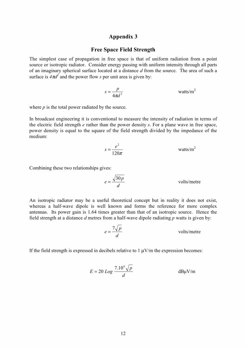
Free Space Field Strength The simplest case of propagation in free space is that of uniform radiation from a point source or isotropic radiator. Consider energy passing with uniform intensity through all parts of an imaginary spherical surface located at a distance d from the source. The area of such a surface is 4πd2 and the power flow s per unit area is given by:

24 dps

π= watts/m2

where p is the total power radiated by the source. In broadcast engineering it is conventional to measure the intensity of radiation in terms of the electric field strength e rather than the power density s. For a plane wave in free space, power density is equal to the square of the field strength divided by the impedance of the medium:

π120

2es = watts/m2

Combining these two relationships gives:

d

pe

30= volts/metre

An isotropic radiator may be a useful theoretical concept but in reality it does not exist, whereas a half-wave dipole is well known and forms the reference for more complex antennas. Its power gain is 1.64 times greater than that of an isotropic source. Hence the field strength at a distance d metres from a half-wave dipole radiating p watts is given by:

d

pe

7= volts/metre

If the field strength is expressed in decibels relative to 1 µV/m the expression becomes:

d

pLogE

610.720= dBµV/m

13

Appendix 4

Antenna Calibration The Ground-Reflection Method

This calibration method is applicable over the frequency range 45 – 250 MHz. The principle involves positioning the transmitting and receiving antennas above a flat ground plane clear of any surrounding objects. Under these conditions the field strength at the receiving antenna may be represented by:

e = eo [ 1 + ρ exp jθ + . . . . . . . . . . . . . . . . .]

Direct Reflected Surface wave, Induction field and wave wave secondary ground effects

where

eo is the field that would exist in free space ρ is the reflection coefficient of the ground plane θ is the phase difference due to the difference in path length of the direct and ground reflected waves

The reflection coefficient of the ground is a complex function depending on the electrical constants of the ground and the polarisation and angle of incidence of the wave. For a horizontally polarised wave at small grazing angles, the reflection coefficient for most ground conditions approximates to -1, i.e. the reflected wave is equal in magnitude to the incident wave but undergoes a phase change of 180° on reflection. The surface wave component can be neglected at heights of the order of a wavelength or more.

Providing the antennas are spaced by more than a few wavelengths the induction field effects can also be neglected and, for these conditions, the field is simply the resultant of the direct and ground reflected waves and can be calculated as follows.

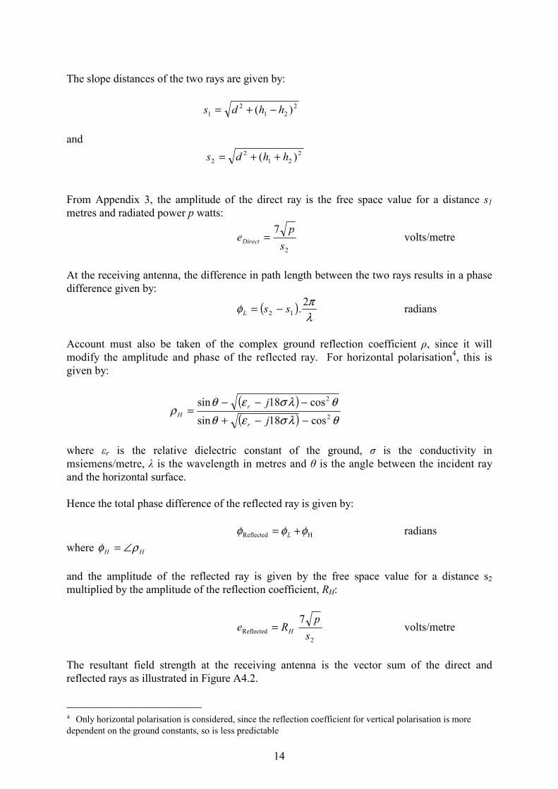
Figure A4.1 shows the path geometry for the direct and reflected rays between transmitting and receiving antennas.

T

θh2

h1 R

s1

s2

d

Fig. A4.1

14

The slope distances of the two rays are given by: 2

212

1 )( hhds −+= and 2

212

2 )( hhds ++= From Appendix 3, the amplitude of the direct ray is the free space value for a distance s1 metres and radiated power p watts:

2

7s

peDirect = volts/metre

At the receiving antenna, the difference in path length between the two rays results in a phase difference given by:

( )λπφ 2.12 ssL −= radians

Account must also be taken of the complex ground reflection coefficient ρ, since it will modify the amplitude and phase of the reflected ray. For horizontal polarisation4, this is given by:

( )( ) θλσεθ

θλσεθρ

2

2

cos18sincos18sin

−−+−−−

=jj

r

rH

where εr is the relative dielectric constant of the ground, σ is the conductivity in msiemens/metre, λ is the wavelength in metres and θ is the angle between the incident ray and the horizontal surface. Hence the total phase difference of the reflected ray is given by: HReflected φφφ += L radians where HH ρφ ∠= and the amplitude of the reflected ray is given by the free space value for a distance s2 multiplied by the amplitude of the reflection coefficient, RH:

2

Reflected

7s

pRe H= volts/metre

The resultant field strength at the receiving antenna is the vector sum of the direct and reflected rays as illustrated in Figure A4.2.

4 Only horizontal polarisation is considered, since the reflection coefficient for vertical polarisation is more dependent on the ground constants, so is less predictable

15

φReflected

e Reflected

e Resultant

e Direct

Fig. A4.2

The foregoing calculations do not lend themselves to pocket calculator processing and a small program, 2RayCalc.exe, has been written to facilitate the calculation of the relevant field strengths when using the Calibration Run. The program runs under windows and has a graphical display, shown in Fig. A4.3, which helps to visualise the expected variation in level along the run. It calculates both the horizontally and vertically polarised field strengths as well as the free space values. With the Calibration Run method, only the horizontally polarised field strength is measured but the program can be used for simulating other situations where direct and ground/sea reflected signals interact (e.g. tidal fading).

Fig. A4.3 2RayCalc.exe display

16

Fig. A4.4 shows a comparison between the predicted horizontally polarised field strength and measurements made using a λ/2 dipole at 30, 40, 50, 60 and 70 metres along the Calibration Run. Using these measured results, the average gain of the dipole was calculated to be -0.6 dBd. The expected gain of a λ/2 dipole is 0 dBd but the antenna used had 75/50Ω balun and a short connecting feeder and the combined loss was about 0.5 dB.

70

80

90

100

20 30 40 50 60 70 80Distance, metres

Fiel

d st

reng

th, d

B µµ µµV/

m

Theoretical field strength

Measured field strength

Frequency: 222 MHzERP: 12.5 dBmHt: 2.3 metresHr: 3.0 metresεr: 4ρ: 10 mS/m

Fig. A4.4 Measured and theoretical field strength variation at 222 MHz

For maximum accuracy, it is best to adjust the height parameters so that a field strength maximum occurs along the run, as opposed to a field strength minimum. The values used will be frequency dependent and Table A4.1 gives suggested heights to use for frequencies in Bands I to III.

Table A4.1 Typical parameters and field strengths associated

with the Ground Reflection Method

Freq (MHz) ERP (dBm) Ht (m) Hr (m) d (m) Eh (dBuV/m)50.0 13.0 10.0 5.0 30.0 94.5

40.0 91.850.0 89.160.0 86.670.0 84.4

100.0 13.0 10.0 3.0 30.0 93.840.0 92.350.0 90.160.0 87.970.0 86.2

200.0 13.0 5.0 3.0 30.0 94.140.0 92.950.0 90.760.0 88.470.0 86.2

17

Appendix 5

Antenna Calibration The Diffraction Screen Method

At UHF, the Ground Reflection method is less reliable. At these shorter wavelengths, errors due to inaccuracies in positioning the antenna or unevenness of the ground are more likely to become significant, and it is preferable to use a method which eliminates ground reflections. This can be achieved by using a vertical wire mesh screen between the transmitting and receiving antennas. The screen, which is opaque at UHF, cuts out ground reflections and causes the direct signal to be diffracted over its upper edge. This sets up a standing wave pattern such that the field strength varies with height as shown in Fig. A5.1. The field obtained behind a screen can be calculated by classical theory for diffraction over a knife edge, but for the purposes of antenna calibration this is not necessary.

In the region where the direct path is optically clear of the obstacle, the field fluctuates in an oscillatory manner and, as the clearance is increased, the field strength approaches the free space value. For example, the mean of the first maximum and minimum values is within 1 dB of the free space value, but the mean of the second maximum and minimum values is within 0.2 dB of it. In practice, the mean of the second maximum and minimum values can be taken as being representative of the free space field strength at the receiving site. The value of this free space field is easily calculated from the distance between the transmitting and receiving antennas and the ERP using the equation given in Appendix 3.

Fig. A5.1 Field strength variation behind a diffraction screen

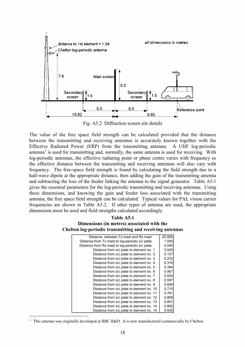
The appropriate conditions can be readily achieved at UHF using reasonable physical dimensions for the screen. This method is less applicable to VHF because a very large screen would be required. The layout and dimensions are shown in Fig. A5.2. The smaller secondary screens located either side of the main screen are to reduce the effect of ground reflections.

18

Fig. A5.2 Diffraction screen site details

The value of the free space field strength can be calculated provided that the distance between the transmitting and receiving antennas is accurately known together with the Effective Radiated Power (ERP) from the transmitting antenna. A UHF log-periodic antenna5 is used for transmitting and, normally, the same antenna is used for receiving. With log-periodic antennas, the effective radiating point or phase centre varies with frequency so the effective distance between the transmitting and receiving antennas will also vary with frequency. The free-space field strength is found by calculating the field strength due to a half-wave dipole at the appropriate distance, then adding the gain of the transmitting antenna and subtracting the loss of the feeder linking the antenna to the signal generator. Table A5.1 gives the essential parameters for the log-periodic transmitting and receiving antennas. Using these dimensions, and knowing the gain and feeder loss associated with the transmitting antenna, the free space field strength can be calculated. Typical values for PAL vision carrier frequencies are shown in Table A5.2. If other types of antenna are used, the appropriate dimensions must be used and field strengths calculated accordingly.

Table A5.1 Dimensions (in metres) associated with the

Chelton log-periodic transmitting and receiving antennas Distance between Tx mast and Rx mast 20.850

Distance from Tx mast to log-periodic s/c plate 1.000Distance from Rx mast to log-periodic s/c plate 0.040

Distance from s/c plate to element no. 1 0.040Distance from s/c plate to element no. 2 0.137Distance from s/c plate to element no. 3 0.232Distance from s/c plate to element no. 4 0.316Distance from s/c plate to element no. 5 0.394Distance from s/c plate to element no. 6 0.467Distance from s/c plate to element no. 7 0.534Distance from s/c plate to element no. 8 0.597Distance from s/c plate to element no. 9 0.656Distance from s/c plate to element no. 10 0.710Distance from s/c plate to element no. 11 0.761Distance from s/c plate to element no. 12 0.808Distance from s/c plate to element no. 13 0.851Distance from s/c plate to element no. 14 0.892Distance from s/c plate to element no. 15 0.930

5 This antenna was originally developed at BBC R&D. It is now manufactured commercially by Chelton.

19

Table A5.2 Parameters and field strengths

associated with the diffraction screen

Channel

PAL vision carrier

frequency (MHz)

Feeder loss (dB)

Cheltonlog-periodic gain (dBd)

Distance between phase centres (metres)

Free space field strength1

(dBµV/m) 21 471.25 1.87 8.05 19.25 87.422 479.25 1.88 8.08 19.22 87.423 487.25 1.90 8.10 19.18 87.424 495.25 1.91 8.10 19.16 87.425 503.25 1.93 8.10 19.13 87.426 511.25 1.95 8.10 19.10 87.427 519.25 1.98 8.10 19.06 87.428 527.25 1.99 8.10 19.03 87.429 535.25 2.00 8.11 19.00 87.430 543.25 2.02 8.12 18.97 87.431 551.25 2.05 8.15 18.95 87.432 559.25 2.08 8.18 18.92 87.533 567.25 2.10 8.20 18.89 87.534 575.25 2.10 8.20 18.86 87.535 583.25 2.11 8.20 18.84 87.536 591.25 2.12 8.20 18.80 87.537 599.25 2.14 8.20 18.78 87.538 607.25 2.15 8.20 18.75 87.539 615.25 2.16 8.21 18.72 87.540 623.25 2.18 8.22 18.70 87.541 631.25 2.20 8.25 18.68 87.542 639.25 2.21 8.27 18.65 87.543 647.25 2.24 8.30 18.62 87.644 655.25 2.25 8.30 18.60 87.645 663.25 2.25 8.30 18.59 87.646 671.25 2.26 8.30 18.58 87.647 679.25 2.28 8.30 18.55 87.648 687.25 2.30 8.30 18.53 87.549 695.25 2.30 8.30 18.51 87.650 703.25 2.30 8.28 18.49 87.551 711.25 2.31 8.20 18.48 87.552 719.25 2.32 8.10 18.45 87.453 727.25 2.35 8.02 18.43 87.354 735.25 2.37 7.95 18.42 87.255 743.25 2.40 7.86 18.40 87.156 751.25 2.40 7.80 18.39 87.057 759.25 2.41 7.80 18.37 87.058 767.25 2.42 7.80 18.35 87.059 775.25 2.45 7.80 18.33 87.060 783.25 2.46 7.80 18.32 87.061 791.25 2.49 7.80 18.30 87.062 799.25 2.50 7.80 18.29 87.063 807.25 2.51 7.80 18.28 87.064 815.25 2.52 7.80 18.26 87.065 823.25 2.53 7.80 18.25 86.966 831.25 2.55 7.80 18.22 86.967 839.25 2.58 7.80 18.21 86.968 847.25 2.60 7.80 18.20 86.9

1 for a signal generator output of 0 dBm