NASA/TM-2006-213678

Reconfigurable Control with Neural Network Augmentation for a Modified F-15 Aircraft

John J. Burken and Peggy Williams-HayesNASA Dryden Flight Research CenterEdwards, California

John T. KaneshigeNASA Ames Research CenterMoffett Field, California

Susan J. StachowiakNASA Johnson Space CenterHouston, Texas

April 2006

https://ntrs.nasa.gov/search.jsp?R=20060018301 2018-07-27T00:19:13+00:00Z

NASA STI Program ... in ProfileSince its founding, NASA has been dedicated to the advancement of aeronautics and space science. The NASA scientific and technical information (STI) program plays a key part in helping NASA maintain this important role.

The NASA STI program is operated under the auspices of the Agency Chief Information Officer. It collects, organizes, provides for archiving, and disseminates NASA’s STI. The NASA STI program provides access to the NASA Aeronautics and Space Database and its public interface, the NASA Technical Report Server, thus providing one of the largest collections of aeronautical and space science STI in the world. Results are published in both non-NASA channels and by NASA in the NASA STI Report Series, which includes the following report types:

TECHNICAL PUBLICATION. Reports of completed research or a major significant phase of research that present the results of NASA programs and include extensive data or theoretical analysis. Includes compilations of significant scientific and technical data and information deemed to be of continuing reference value. NASA counterpart of peer- reviewed formal professional papers but has less stringent limitations on manuscript length and extent of graphic presentations.

TECHNICAL MEMORANDUM. Scientific and technical findings that are preliminary or of specialized interest, e.g., quick release reports, working papers, and bibliographies that contain minimal annotation. Does not contain extensive analysis.

CONTRACTOR REPORT. Scientific and technical findings by NASA-sponsored contractors and grantees.

•

•

•

CONFERENCE PUBLICATION. Collected papers from scientific and technical conferences, symposia, seminars, or other meetings sponsored or cosponsored by NASA.

SPECIAL PUBLICATION. Scientific, technical, or historical information from NASA programs, projects, and missions, often concerned with subjects having substantial public interest.

TECHNICAL TRANSLATION. English- language translations of foreign scientific

and technical material pertinent to NASA’s mission.

Specialized services also include creating custom thesauri, building customized databases, and organizing and publishing research results.

For more information about the NASA STI program, see the following:

Access the NASA STI program home page at http://www.sti.nasa.gov.

E-mail your question via the Internet to help@sti.nasa.gov.

Fax your question to the NASA STI Help Desk at (301) 621-0134.

Phone the NASA STI Help Desk at (301) 621-0390.

Write to: NASA STI Help Desk NASA Center for AeroSpace Information 7121 Standard Drive Hanover, MD 21076-1320

•

•

•

•

•

•

•

NASA/TM-2006-213678

Reconfigurable Control with Neural Network Augmentation for a Modified F-15 Aircraft

John J. Burken and Peggy Williams-HayesNASA Dryden Flight Research CenterEdwards, California

John T. KaneshigeNASA Ames Research CenterMoffett Field, California

Susan J. StachowiakNASA Johnson Space CenterHouston, Texas

April 2006

National Aeronautics andSpace Administration

Dryden Flight Research CenterEdwards, California 93523-0273

NOTICEUse of trade names or names of manufacturers in this document does not constitute an official endorsement of such products or manufacturers, either expressed or implied, by the National Aeronautics and Space Administration.

Available from the following:

NASA Center for AeroSpace Information National Technical Information Service 7121 Standard Drive 5285 Port Royal RoadHanover, MD 21076-1320 Springfield, VA 22161-2171(301) 621-0390 (703) 605-6000

ABSTRACT

Description of the performance of a simplified dynamic inversion controller with neural network augmentation follows. Simulation studies focus on the results with and without neural network adaptation through the use of an F-15 aircraft simulator that has been modified to include canards. Simulated control law performance with a surface failure, in addition to an aerodynamic failure, is presented. The aircraft, with adaptation, attempts to minimize the inertial cross-coupling effect of the failure (a control derivative anomaly associated with a jammed control surface). The dynamic inversion controller calculates necessary surface commands to achieve desired rates. The dynamic inversion controller uses approximate short period and roll axis dynamics. The yaw axis controller is a sideslip rate command system. Methods are described to reduce the cross-coupling effect and maintain adequate tracking errors for control surface failures. The aerodynamic failure destabilizes the pitching moment due to angle of attack. The results show that control of the aircraft with the neural networks is easier (more damped) than without the neural networks. Simulation results show neural network augmentation of the controller improves performance with aerodynamic and control surface failures in terms of tracking error and cross-coupling reduction.

NOMENCLATURE

A state

ay lateral acceleration, ft/sec2

B control

Ba neural network basis function

C neural network input (roll, pitch, and yaw axis)

Cmα pitching moment due to α , 1/deg

dap roll stick input, in

deg degree

dep pitch stick input, in

drp rudder pedal input, in

dt change in time, sec

e x− exponential function

G adaptation gain

Gen 2 generation 2

i integral

2

IFCS Intelligent Flight Control System

K constant gain

K pi constant integral roll gain, deg/deg/sec

K qi constant integral pitch gain, deg/deg/sec

K ped pilot pedal gain, deg/in

K pp constant proportional roll gain, deg/sec

K qp constant proportional pitch gain, deg/sec

Kzp proportional gain, deg

Kzi integral gain, deg

L neural network error-modification damping term

L1 rolling moment, ft-lbf

Lα lift curve slope, rad/sec

M1 pitching moment, ft-lbf

NN neural network

ny lateral acceleration, g

nz normal acceleration, g

p body axis roll rate, deg/sec

p body axis roll acceleration, deg/sec

p proportional

PI proportional and integral

q pitch rate, deg/sec

q pitch acceleration, deg/sec2

r yaw rate, deg/sec

s Laplace operator

sec second

T transpose

U controller command

3

Uerr neural network error compensation terms

Vt total velocity, ft/sec

W neural network weights

W rate of change in the neural network weights

x vector of aircraft states

x rate of change of the state x

z p, q, or r variable

6-DOF six-degree-of-freedom

α angle of attack, deg

β angle of sideslip, deg

β time rate of change of angle of sideslip, deg/sec

δa roll axis surface deflection, deg

δe pitch axis surface deflection, deg

ζsp short period damping, rad/sec

θ pitch angle, deg

τr rise time, sec

φ bank angle, deg

ωsp short period frequency, rad/sec

Subscripts

ad adaptation

c command

dd direct derivative

err error

est estimate

int integrator

k step frame

lat lateral

4

lon longitudinal

ref reference

sp short period

INTRODUCTION

The objective of the NASA Intelligent Flight Control System (IFCS) program is to develop and flight-test schemes that enhance control during primary control surface failures or aerodynamic changes resulting from failures or modeling errors. The first flight phase, known as generation one (Gen 1), required aerodynamic parameter identification and is not discussed in this report (please see reference 1 for a discussion on the Gen 1 flight phase). The second flight phase, known as generation two (Gen 2), evaluates a neural flight control system that can provide adaptive control without explicit parameter identification. The Gen 2 approach does not require information on the nature or the extent of the failure, knowledge of the control surface positions, or information on aerodynamic failures or unmodeled parameters. The Gen 2 tracking controller adds direct adaptive neural network signals to the control law (references 2 – 6). These neural networks are used to generate command augmentation signals to compensate for errors caused by unmodeled dynamics, including dynamics resulting from damage or failure. Flight demonstration began in early 2006 on the NASA F-15 aircraft (originally built by McDonnell Douglas Aircraft Company, now The Boeing Phantom Works, St. Louis, Missouri), tail number 837. The F-15 six-degree-of-freedom (6-DOF) simulator that was used in the evaluation test compared stabilator and canard failure compensation with the neural network algorithm. A canard failure emulates a change in pitching moment due to angle of attack, Cmα , and is considered an aerodynamic malfunction caused by modeling errors or damage. This type of failure is discussed in a subsequent section of this report entitled, “Simulation Results,” “ A Matrix Failure (Aerodynamic Failure).”

The specific objectives of Gen 2 are to (1) implement and fly a direct adaptive neural network–based flight controller, (2) demonstrate the ability of the system to adapt to simulated system failures by suppressing transients associated with the failure, (3) reestablish sufficient control and handling of the vehicle for safe recovery, and (4) provide flight experience for the development of verification and validation processes for flight-critical neural network software.

DESCRIPTION OF THE RESEARCH VEHICLE

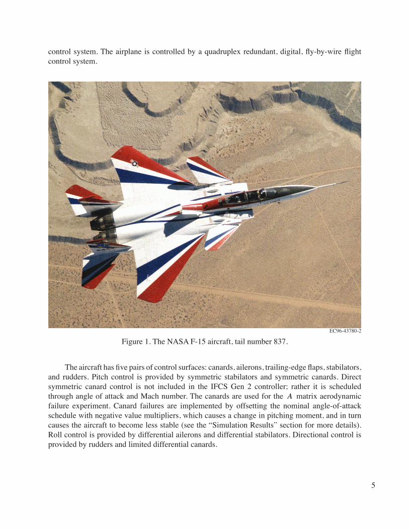
A preproduction F-15B aircraft, which has been highly modified to support various test programs, is used in this research project. The most visible modification is the addition of a set of canards near the pilot station (figure 1). The canards are a set of modified horizontal stabilators from an F-18 aircraft (originally built by McDonnell Douglas Aircraft Company, now The Boeing Phantom Works, St. Louis, Missouri). The propulsion system consists of two F100-PW-229 engines (Pratt & Whitney, West Palm Beach, Florida), each equipped with an axisymmetric thrust-vectoring pitch-yaw balance beam nozzle (ref. 1). The thrust-vectoring feature is not used in the Gen 2 controller, and the canards are not used for direct longitudinal control in the Gen 2

5

control system. The airplane is controlled by a quadruplex redundant, digital, fly-by-wire flight control system.

Figure 1. The NASA F-15 aircraft, tail number 837.

The aircraft has five pairs of control surfaces: canards, ailerons, trailing-edge flaps, stabilators, and rudders. Pitch control is provided by symmetric stabilators and symmetric canards. Direct symmetric canard control is not included in the IFCS Gen 2 controller; rather it is scheduled through angle of attack and Mach number. The canards are used for the A matrix aerodynamic failure experiment. Canard failures are implemented by offsetting the nominal angle-of-attack schedule with negative value multipliers, which causes a change in pitching moment, and in turn causes the aircraft to become less stable (see the “Simulation Results” section for more details). Roll control is provided by differential ailerons and differential stabilators. Directional control is provided by rudders and limited differential canards.

EC96-43780-2

6

DESCRIPTION OF THE GENERATION 2 CONTROLLER

The general control scheme of the Gen 2 controller is based on an adaptive neural controller that cancels errors associated with the dynamic inversion of the model. Initially, constant values of aerodynamic stability and control derivatives for a fixed condition in the flight envelope are used for model inversion. In addition, desired handling qualities are achieved with low-order reference models, which are based on pilot preferences (reference 7). The yaw axis controller is not a reference-based controller, but rather a classical yaw system. Figure 2 shows the Gen 2 control structure that uses a direct adaptive control method. The yaw axis controller, which has an adaptation signal added to the classical yaw command, is discussed in a subsequent section of this report entitled, “Classical Yaw Axis Controller” (see figure 3).

prefqref

perrqerr

UpddUqdd

U = B–1(x – Ax)

UpadUqadUrad

pcqc UReference

modelsPI-error

compensator

Error-based inputs for controller adaption

Error-based adaption law

State-based inputs for A matrix failures

Control-based inputs for B matrix failures

Dynamicinverse and

β

Virtual actuator commands

Sensors

060020

+

–

+

+•• •

•

pref

qref•

•

+

–

On-line learningnetworks

Pilotinputs

Figure 2. Generation 2 architecture in which the inversion is applied to the B matrix.

rerrKped10

s+10 ++ +

+

–

Pilotpedal,

drp

060021Washout

filter

Yawcommand

Yaw axisneural network

signal Urad

ny feedback

ss+0.5 K β

Kny

β••

Figure 3. Yaw axis controller with neural network summing point.

7

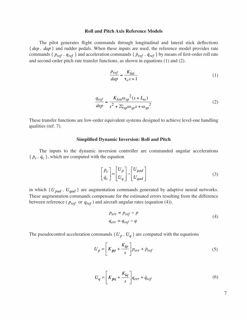
Roll and Pitch Axis Reference Models

The pilot generates flight commands through longitudinal and lateral stick deflections { dep , dap } and rudder pedals. When these inputs are used, the reference model provides rate commands { pref , qref } and acceleration commands { pref , qref } by means of first-order roll rate and second-order pitch rate transfer functions, as shown in equations (1) and (2).

pdap

Ks

ref lat

r=

+τ 1

qdep

K s L

s sref lon sp

sp sp sp=

+

+ +

ω

ζ ω ω

α2

2 22

( )

These transfer functions are low-order equivalent systems designed to achieve level-one handling qualities (ref. 7).

Simplified Dynamic Inversion: Roll and Pitch

The inputs to the dynamic inversion controller are commanded angular accelerations { pc , qc }, which are computed with the equation

pc

qc

⎡

⎣⎢

⎤

⎦⎥ =

Up

Uq

⎡

⎣⎢⎢

⎤

⎦⎥⎥−Upad

Uqad

⎡

⎣⎢⎢

⎤

⎦⎥⎥

in which {U pad , Uqad } are augmentation commands generated by adaptive neural networks. These augmentation commands compensate for the estimated errors resulting from the difference between reference ( pref or qref ) and aircraft angular rates (equation (4)).

p p p

q q qerr ref

err ref

= −

= −

The pseudocontrol acceleration commands {U p , Uq } are computed with the equations

Up = K pp +Kip

s

⎡

⎣⎢

⎤

⎦⎥ perr + pref

Uq = K pq +Kiq

s

⎡

⎣⎢

⎤

⎦⎥qerr + qref

(1)

(2)

(3)

(4)

(5)

(6)

8

in which K p and Ki are proportional and integral constants, respectively, for each axis. Figure 2 shows the computation process for the pseudocontrol acceleration commands. The simplified dynamic inversion algorithm inverts a B matrix with states for modeling the short period and roll modes. To protect against a poorly ranked B matrix, the inversion is generated by a pseudoinverse (equation (7)).

BB B B

B B

T T

T− =

∗ ∗

∗1 Adjoint

Determinant( )( )

The inversion is used to determine necessary control surface deflections {δa , δe }. Control surface commands {δac

, δec} are obtained with the equation

δacδec

⎡

⎣⎢⎢

⎤

⎦⎥⎥= B

−1 pc − L1qc − M1

⎡

⎣⎢

⎤

⎦⎥

in which B is the state space system control matrix and the terms { pc − L1 , qc − M1} are the differences between input acceleration commands and actual plant acceleration contributions { L1, M1 }. These plant contributions are calculated from the appropriate states for modeling the short period and roll mode dynamics.

Classical Yaw Axis Controller

The original research controller was a simplified dynamic inversion controller used for all three control axes: roll, pitch, and yaw. The proportional and integral (PI) gains of this controller were tuned to achieve linear stability robustness and aeroservoelastic (ASE) mode attenuation for the nominal (no-failure) case. When the original dynamic inverse controller was tested with locked stabilator failure simulations, significant lateral acceleration, ny , and angle-of-sideslip, β , excursions resulting from lateral stick inputs were noted. Angle-of-sideslip excursions also were noted with pitch stick input (pitch-yaw cross-coupling). For no-failure cases, pilots typically prefer very little yaw with a roll input.

Subsequent redesigns of the simplified dynamic controller with or without neural networks were not able to modify this behavior, and pilots continued to provide negative comments from simulation sessions. Therefore, to reduce the lateral accelerations and sideslip excursions, the original research controller was modified so that the lateral and directional axes would be decoupled. This modification was accomplished through the use of a sideslip angle rate of change term, β , as the primary feedback, which produced a classical controller for the yaw axis, while the original dynamic inversion controller was still used for the pitch and roll axes.

(7)

(8)

9

The final research controller thus is a hybrid controller that uses a simplified dynamic inversion in the longitudinal and lateral axes and a classical controller in the directional axis. This modification was necessary to obtain reasonable flying qualities in the presence of a simulated failure and remain within a limited project schedule. The β command system does not require angle of sideslip in the relationship. Although sideslip can be measured with a vane or inertial navigation system (INS), β should not be derived by differentiating sideslip. Because the sideslip signal is noisy and differentiating, it would amplify the noise (reference 8). Instead, β can be calculated from measurable parameters and sensors by means of equation (9).

β = psin(α) − r cos(α) +g

Vtcos(θ)sin(φ) +

ay

Vt

Figure 3 shows the yaw axis controller. The directional yaw controller includes a washout filter on β and is summed with a proportional gain, Kny , on ny . As the figure shows, the yaw axis neural network contribution is summed with the yaw command after the β PI controller.

Adaptive Neural Network

The purpose of the neural network system is to accommodate large errors that are not anticipated in the nominal control law design phase. In a failed flight condition or configuration ( A or B matrix), errors will develop that are larger than expected. The adaptive neural network operates in conjunction with the error of the control system. By recognizing patterns in the behavior of the error, the neural networks can learn to remove the error biases through control augmentation commands (fig. 2).

The adaptation signal attempts to remove errors in the neural flight control system to improve handling qualities in the presence of unknown failures. The neural network that provides this online adaptation scheme is known as “sigma pi.” Figure 4 depicts a simple single hidden layer sigma pi network. The name “sigma pi” is derived from the underlying equations of the network that sum ( • ) the products (≠ ) of the inputs to the neural network with their associated weights. The weights of the neural network, W , are determined by a training algorithm, also known as an adaptation or learning rule. Learning involves adjusting these weights so that the network has a valid relationship between the inputs and outputs, and in turn, minimizes the error.

Because a neural network is designed to recognize patterns between inputs and errors, the selected inputs must provide enough coverage for the network to be able to capture the behavior of the error. If too many inputs exist, however, the neural network may not be able to adapt quickly enough for practical application. Although the adaptation gain can be used to increase the rate of adaptation, it can cause large transients in the neural network outputs when it becomes too big. These transients are caused by spikes and sometimes sign changes in the network weights, which are often encountered before the network converges to a learned state.

(9)

10

060022

1

Uad

Uad is the NN output to roll,pitch, and yaw axis:Upad, Uqad, and Urad

W0

W1

W2

W3

W4

x1

x2

x3

π

Σπ

π

π

π

1 neuron with 3 inputs and a bias:

Uad = W01 + W1x1 + W2x2 +W3x3 + W4x1x3

f(x) = –––––––(1–e–x)(1+e–x)

Figure 4. Simple sigma pi neural network structure ( • = sum, ≠ = product).

With piloted aircraft, the neural network must be capable of adapting quickly enough to assist pilots in controlling a damaged aircraft; however, the neural network also should avoid transients that could overload the structure and interfere with the pilot’s ability to control the aircraft. As a result of these constraints, input selection becomes a critical factor for successful implementation of a neural network–based flight control system. The input categories used in this study are aircraft modeling, bias, cross-coupling, and acceleration.

Aircraft Modeling Inputs

The estimated angle-of-attack and sideslip inputs originally were included to capture aircraft modeling effects. For this evaluation, however, the sideslip input was removed, because it did not appear to have a significant effect. Furthermore, previous studies have shown that caution must be used when incorporating aircraft attitude inputs such as pitch and bank angles. In some cases, these inputs did not receive sufficient excitation for effective pattern recognition until various maneuvers were initiated. This problem was especially apparent in cases involving failures in which the network learned to adapt primarily during straight and level flight. When a maneuver eventually was performed, the transients often were disconcerting to pilots, because they thought that the network already had learned to handle the failure. Although the network weights eventually converged again, the transients continued to occur at the critical moment of maneuver execution.

11

Bias Inputs

Bias inputs provide a dual purpose. In terms of sigma pi neural networks, a bias within each input category ensures that each input is represented in the vector of basis functions after the nested Kronecker product. In addition, one of the basis functions becomes the product of the biases. The purpose of this bias term is to compensate for out-of-trim conditions caused by damage or failures. For example, in the case of an offset right stabilator failure, the integrators in both the pitch and roll axes must build up to compensate for the offset. Provided that the integrated error remains nonzero, it will have an effect on the adaptation law and cause the weights to adapt. As a result, the purpose of the bias term is to drive the integrated error back down to zero in the event of out-of-trim conditions.

Cross-Coupling Inputs

The purpose of cross-coupling inputs is to allow the neural networks to learn how one axis may affect another axis. Although one of the functions of dynamic inversion is to decouple the axes, coupling can be reintroduced by events such as control surface failures. For example, in the case of a right stabilator failure, longitudinal stick commands can induce roll. Similarly, lateral stick commands can induce pitch.

To capture control-induced cross-coupling effects, off-axis angular acceleration commands were incorporated as neural network inputs. These acceleration commands excluded the neural adaptive augmentation term to avoid cross-coupled adaptive feedback. Squashing functions were used to normalize the acceleration inputs.

Acceleration Inputs

During a failure, the flight control surface can introduce out-of-trim conditions and also can affect the overall control power of the vehicle. With a right stabilator failure, only the left stabilator remains available for longitudinal control. As a result, more left stabilator deflection is necessary to achieve the same angular acceleration. The acceleration inputs were represented by the on-axis acceleration commands, Udd . Remember that the Udd is the PI controller signal that originates from the compensator.

Application of the Adaptive Neural Network

The adaptive neural network implemented for the flight test is divided into three separate networks, one each for the pitch, roll, and yaw axes. Inputs to the network consist of control commands, sensor feedback, and bias terms. The number of inputs to each individual neural network vary; the roll axis uses six, the pitch axis uses seven, and the yaw axis uses ten. Table 1 presents the inputs for each neural network. The output of each neural network is an angular acceleration command that augments the control signal from the research controller for each axis. To couple the three networks, pitch information is included in the roll and yaw neural networks, and some roll axis signals are included in the pitch and yaw neural networks.

12

Table 1. Neural network input elements (see symbol C in equation (10)).

Roll axis network Pitch axis network Yaw axis network

pUdd , roll control direct derivative signal

qUdd , pitch control direct derivative signal

dap, roll stick

perr , roll control error qerr , pitch control error dep, pitch stick

perrint , roll integrator error qerrint , pitch integrator error drp, rudder pedal

qUdd , pitch control direct derivative signal

pUdd , roll control direct derivative signal

βest , angle of sideslip rate estimate

rUdd , yaw control direct derivative signal

rUdd , yaw control direct derivative signal

φ , bank angle, rad

pbias , roll axis bias α , angle of attack, rad rUdd , yaw control direct derivative signal

qbias , pitch axis biaspUdd , roll control direct

derivative signal

qUdd , pitch control direct derivative signal

rad k( )−1 , yaw axis neural network output delayed

one frame

rbias , yaw axis bias

The neural network output, Uad , is the control augmentation command comprised of three components: roll, pitch, and yaw (U pad , Uqad , Urad ). This neural network output is computed with equation (10) (see fig. 2).

U W B CadT

a=

The vector of basis function, Ba , is computed from the inputs in each signal input category by means of a product. Table 1 shows the input vector, C . The network weights, W , are computed by an adaptation law, which includes an adaptation gain, G , and an error-modification term, L . The error-modification term helps contain the parameter growth of the weights and can be considered a damping term. The final adaptation law is

W = −G UerrBa + LUerrW( )dt

(10)

(11)

13

in which W is the weight increment for the current time step; W is the weight from the previous time-step; dt is the time-step, which is 0.0125 seconds (80 Hz); G is the adaptation gain, which is sometimes called the learning rate; and Uerr is the error compensation. This weight calculation is currently implemented in the Gen 2 system.

The squashing function used to normalize inputs to the neural network is a sigmoid function and has the form (also shown in fig. 4)

f x e ex x( ) ( ) / ( )= − +− −1 1

This squashing function is used on all the neural network inputs listed in table 1.

The adaptation law is computed as a function of the PI controller gains and tracking error ( perr , qerr , and rerr equated to err in equation (13)).

U Kz err Kz errerr = +≡i p

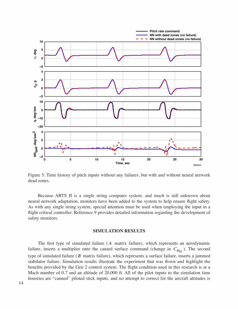
This computation allows the neural networks to work in conjunction with the dynamic inversion PI controllers. Furthermore, because the adaptation gain can be used to specify the overall rate of adaptation, the adaptation law gains can be viewed as specifying the relative rates of adaptation. Concerning the dead zones applied to the error compensation, to keep the neural network from constantly adapting to small errors, dead zones are included on all three axes. The dead zones were applied to the Uerr signals and size was determined by means of the 6-DOF simulators. Figure 5 shows a time history of pitch inputs without any failures but with and without the neural network dead zones. Note that the pitch rate response is the same with or without dead zones but the pitch neural network output keeps growing without dead zones because of small errors in the pitch command system.

Flight Control Computer and Airborne Research Test System II

The flight control system algorithms (control laws) reside in the flight control computer (FCC), but the adaptive neural networks reside in a single string research computer where information is passed over a 1553 data bus. The research computer is called the Airborne Research Test System II (ARTS II), but the bus information is not instantaneously transferred from the FCC and ARTS II and back again. Frame delays are the result of computational requirements of the control algorithms, neural network algorithms, signal lineup on the 1553 data bus, and other asynchronous tasks. The delay was determined to be 0.05 seconds, which is four frame delays. When these neural network algorithms (or other neural network algorithms) are embedded into a production quadruplex redundant, digital, fly-by-wire flight control system, this delay does not exist. The neural network sensor inputs are quadruplex redundant and thus ensure a high degree of redundancy.

(12)

(13)

14

−5

0

5

10

α,d

eg

−2

0

2

4

n z,g

−20

−10

0

10

q,de

g/se

c

0 5 10 15Time, sec

060023

20 25 30−2

0

2

4

NN

qad,

deg/

sec2

Pitch rate commandNN with dead zones (no failure)NN without dead zones (no failure)

Figure 5. Time history of pitch inputs without any failures, but with and without neural network dead zones.

Because ARTS II is a single string computer system, and much is still unknown about neural network adaptation, monitors have been added to the system to help ensure flight safety. As with any single string system, special attention must be used when employing the input in a flight critical controller. Reference 9 provides detailed information regarding the development of safety monitors.

SIMULATION RESULTS

The first type of simulated failure ( A matrix failure), which represents an aerodynamic failure, inserts a multiplier onto the canard surface command (change in Cmα ). The second type of simulated failure ( B matrix failure), which represents a surface failure, inserts a jammed stabilator failure. Simulation results illustrate the experiment that was flown and highlight the benefits provided by the Gen 2 control system. The flight condition used in this research is at a Mach number of 0.7 and an altitude of 20,000 ft. All of the pilot inputs to the simulation time histories are “canned” piloted stick inputs, and no attempt to correct for the aircraft attitudes is

15

added to the piloted inputs. This “canned” pilot input method was used only for comparison purposes and is not intended for flight test at this point in time. Because the controller is a rate command system, attitudes such as bank angle, φ , are used only for comparison and disturbance rejection trade-off studies. For instance, when a failure is imparted on the aircraft and the resulting attitudes change minimally, the control system is considered to have good robustness properties.

A Matrix Failure (Aerodynamic Failure)

The first case is an A matrix failure imposed on both the left and right canards, with a multiplier of – 0.5 on the nominal angle-of-attack schedule. This failure forces the canards to a less stable configuration. Figure 6 shows a 30-second time history with three longitudinal pilot stick inputs and a failure imposed at 11 seconds. In the first 10 seconds a normal response demonstrates how the pitch rate follows the commanded pitch rate (represented by the solid black line). The blue lines in fig. 6, which represent the aircraft response when the neural network is inactive, show that after the failure is inserted, the aircraft is stable but experiences two or three overshoots. When the neural network is active (represented by the red lines in fig. 6), the response is better damped and the commanded pitch rate is followed more closely than when the neural network is inactive. By the third pilot input, the neural network response is very close to the commanded pitch rate (represented by the solid black line). The lateral-directional states shown in figure 7 indicate that no changes were caused by the canard failure. This result is expected, because the failure is a purely longitudinal case and has no impact on the lateral-directional axis. Figure 8 shows the neural network contribution to the roll, pitch, and yaw axes in which NN pad , NNqad , and NNrad are the three neural network signal commands. The adaptation activates at 11 seconds (the time at which the failure is imposed) and only the pitch neural network reacts to the failure. All three neural networks are engaged but only the pitch neural network reacts to the error, because all of the error is in the pitch channel. The results demonstrate that with this type of failure the neural networks help with tracking and damping.

Note that a dead zone that allows for small errors without neural network adaptation is included in the neural network design. This dead zone is important, because it keeps the neural networks from constantly changing for small errors.

16

−20

0

20

−10

0

10

−50

0

50

−1

0

1

dap,

in.

dep,

in.

0 5 10 15Time, sec

20 25 30060024

−2

0

2

Pitch rate commandNN offNN on

α,d

egn z

,gq,

deg/

sec

Figure 6. Time history of longitudinal aircraft states of an A matrix canard failure at 11 seconds (multiplier = – 0.5).

17

−1

0

1

p,de

g/se

c

−1

0

1

r,de

g/se

c

−1

0

1

φ,de

g

−1

0

1

β,de

gda

p, in

.

0 5 10 15Time, sec

20 25

060025

30−1

0

1

NN offNN on

Figure 7. Time history of lateral-directional aircraft states of an A matrix canard failure at 11 seconds (multiplier = – 0.5).

18

−1.0

−0.5

0

0.5

1.0N

Npa

d, d

eg/s

ec2

NN offNN on

−100

−50

0

50

100

NN

qad,

deg

/sec

2

5 10 15Time, sec

20 25 30060026

−1.0

−0.5

0

0

0.5

1.0

NN

rad,

deg

/sec

2

Figure 8. Time history of neural network activity of an A matrix canard failure at 11 seconds (multiplier = – 0.5).

B Matrix Failure (Control Surface Failure)

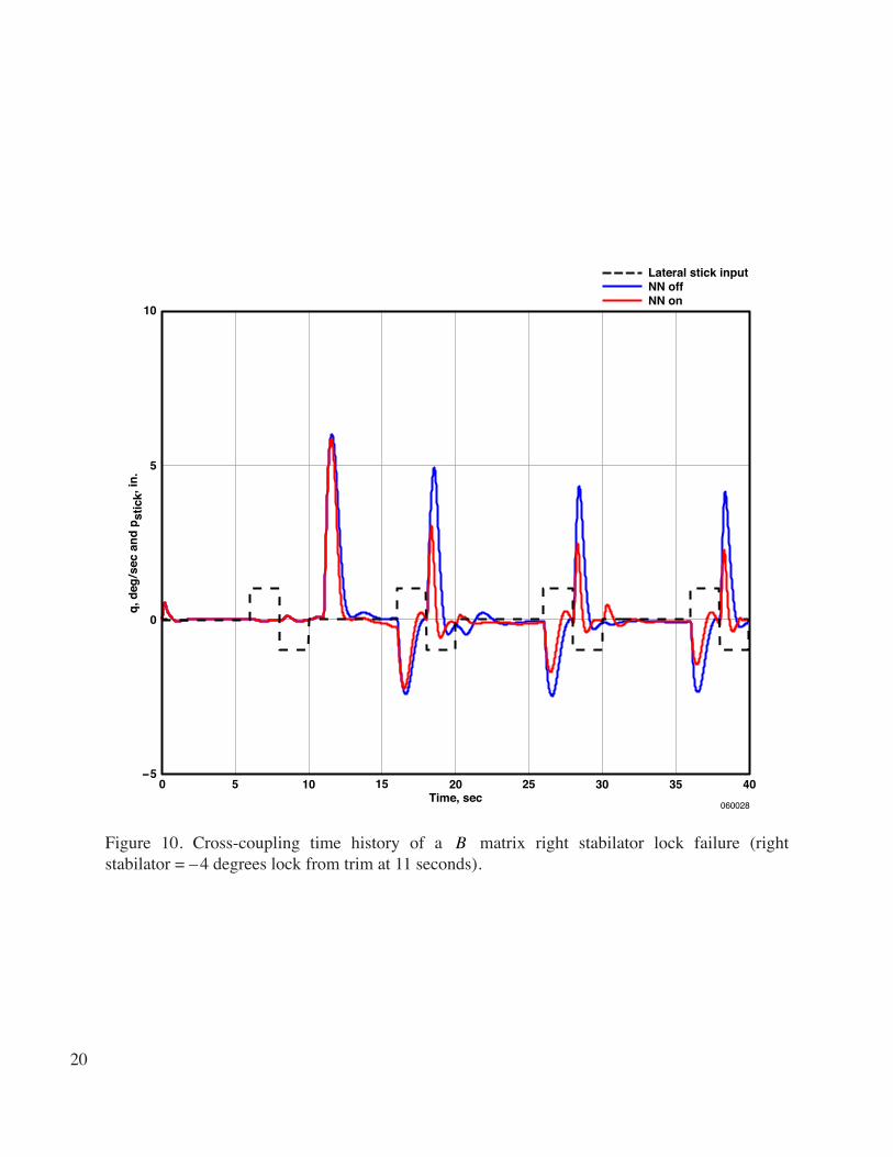
The second case is a B matrix failure, involving a – 4-degree lock from trim, which is imposed on the right stabilator 11 seconds into the simulation run. Figure 9 shows a 40-second time history in which lateral pilot stick inputs are commanded. During the first 10 seconds the pitch rate does not move with the lateral pilot input. This situation is preferred; roll inputs should have little or no impact on longitudinal states. When the stabilator failure is injected at 11 seconds, note that transients occur in angle of attack, normal acceleration, and pitch rate. Initially cross-coupling reduces minimally when the neural networks are active, compared to when the neural networks are inactive, as shown in fig. 9 (see angle of attack and normal acceleration time histories). As the “canned” pilot input resumes at 16 seconds, the neural networks continue to adapt and show improvement over the nonadaptive case. The amount of normal acceleration disturbance during a roll command is approximately 40-percent less when the neural networks are active. Figure 10 shows pitch rate, q , plotted over with the pilot roll stick (represented by the black dashed line). Before the failure very little pitch rate and normal acceleration excursion occur with the roll inputs (first roll doublet). As the neural networks become a significant influence, cross-coupling decreases as the roll stick doublets continue with time.

19

0

5

−2

0

2

−10

0

10

−2

0

2

0 10 15 20Time, sec

25 30 35 40

060027

−1

0

1

5

Zero commandNN offNN on

α,d

egn z

,gq,

deg/

sec

dep,

in.

dap,

in.

Figure 9. Time history of longitudinal aircraft states of a B matrix right stabilator lock failure (right stabilator = – 4 degrees lock from trim at 11 seconds).

20

0 5 10 15 20Time, sec

25 30 35 40060028

−5

0

5

10

q, d

eg/s

ec a

nd p

stic

k, in

.

Lateral stick inputNN offNN on

Figure 10. Cross-coupling time history of a B matrix right stabilator lock failure (right stabilator = – 4 degrees lock from trim at 11 seconds).

21

Figure 11 shows the lateral-directional states from the roll inputs. As previously noted, the inputs are “canned” and no other pilot commands are injected to level the aircraft after the failure. Note that the yaw rate, bank angle, and sideslip excursions are lower when the neural networks are active than when the neural networks are inactive. The roll axis is a roll rate command system (represented by the black solid line on the top plot). During the first commanded doublet no failure occurs and the tracking is good for both cases (neural networks inactive and active). After the failure is activated, the tracking is somewhat better when the neural networks are active than when they are inactive.

−50

0

50

p,de

g/se

c

Roll rate commandNN offNN on

−10

0

10

r,de

g/se

c

−200

0

200

φ,de

g

−2

0

2

β,de

g

0 5 10 15 20Time, sec

25 30 35 40060029

−2

0

2

dap,

in.

Figure 11. Time history of lateral-directional aircraft states of a B matrix right stabilator lock failure (right stabilator = – 4 degrees lock from trim at 11 seconds).

22

Figure 12 shows the neural network contribution commands to the roll, pitch, and yaw axes ( NN pad , NNqad , and NNrad ). An abundance of cross-coupling occurs with this failure, which causes all three neural networks to become active.

0

50

100

150

200

NN

pad,

deg

/sec

2

NN offNN on

0

20

40

60

80

NN

qad,

deg

/sec

2

0 5 10 15 20Time, sec

25 30 35 40060030

−0.03

−0.02

−0.01

0

NN

rad,

deg

/sec

2

Figure 12. Time history of neural network activity of a B matrix right stabilator lock failure (right stabilator = – 4 degrees lock from trim at 11 seconds).

Statistical Method Evaluation Approach

Statistical methods provide another approach for comparing the potential improvements attained from using an adaptive system. The simulator can provide perfect repeatable doublets for the pilot inputs, thus back-to-back comparisons of results with and without neural networks are possible. A pilot is not able to consistently apply the same inputs, however, so performance comparison becomes difficult. When a statistical-based evaluation approach is used, determination of a better (lower error) tracking controller is possible. The tracking errors for the roll, pitch, and yaw axes should be lower with adaptation than without adaptation. The performance of the two controllers (with neural networks inactive and active) has been evaluated by means of trajectory tracking parameters, such as mean and standard deviation of roll rate error, pitch rate error, and yaw axis error. Other evaluation parameters include control surface activity such as surface

23

deflections of canards, stabilators, rudders, and ailerons (ref. 8), and pilot work load such as longitudinal stick, lateral stick, pedal, and throttles. Table 2 lists the values for the trajectory tracking performance parameters. Figure 13 shows the error squared for each axis with the same maneuver as that presented in figs. 9 –12. Figure 13 and table 2 demonstrate a reduction in error and an improvement in tracking, by as much as 50 percent, when the neural networks are active compared to when the neural networks are inactive.

Table 2. Trajectory tracking parameters (deg/sec) of a B matrix right stabilator lock failure.

Parameterperr

(mean)perr

(standard deviation)

qerr (mean)

qerr (standard deviation)

rerr (mean)

rerr (standard deviation)

NN off 7.0667 8.1920 1.1957 1.7549 0.0100 0.0083NN on 3.5455 5.3980 0.6500 1.2814 0.0069 0.0054Tracking error reduction, percent

50.2 34.0 45.6 27.0 29.0 35.0

24

0

500

1000

NN offNN on

0

10

20

30

40

0 5 10 15 20 25 30 35 40060031Time, sec

3 x 10–3

2

1

0

p err

2, d

eg2 /s

ec2

q err

2, d

eg2 /s

ec2

r err

2, d

eg2 /s

ec2

Figure 13. Error squared statistical method approach; time history of a B matrix right stabilator lock failure (right stabilator = – 4 degrees lock from trim at 11 seconds).

SUMMARY OF RESULTS

Simulation results have been presented of a neural network adaptive controller that compensates for errors resulting from aerodynamic and control surface failures. This hybrid controller uses simplified dynamic inversion control for the pitch and roll axes and a classical sideslip rate controller for the yaw axis. The neural network is an on-line direct adaptive algorithm that attempts to drive the error between the reference model and commanded state to zero. An aerodynamic failure and jammed control surface failure have been demonstrated. In both failure cases the controller with neural network augmentation demonstrated improvements compared to the nonadaptive controller without neural network augmentation.

During the aerodynamic failure, the neural networks improved the damping and tracking. During the jammed control surface failure, the neural networks reduced cross-coupling by 40 percent, enabling the pilot to fly to the desired trajectory with fewer tracking errors. The neural networks reduced the tracking errors between 27 and 50 percent.

25

REFERENCES

Williams-Hayes, Peggy S., Selected Flight Test Results for Online Learning Neural Network-Based Flight Control System, NASA/TM-2004-212857, 2004.

Williams-Hayes, Peggy S., Flight Test Implementation of a Second Generation Intelligent Flight Control System, NASA/TM-2005-213669, 2005.

Calise, A. J., S. Lee, and M. Sharma, “Direct Adaptive Reconfigurable Control of a Tailless Fighter Aircraft,” AIAA-98-4108, Aug. 1998.

Rysdyk, Rolf T. and Anthony J. Calise, “Fault Tolerant Flight Control Via Adaptive Neural Network Augmentation,” AIAA-98-4483, Aug. 1998.

Perhinschi, Mario G., Marcello R. Napolitano, Giampiero Campa, Brad Seanor, Srikanth Gururajan, and Gu Yu, “Design and Flight Testing of Intelligent Flight Control Laws for the WVU YF-22 Model Aircraft,” AIAA-2005-6445, Aug. 2005.

Kaneshige, John, John Bull, and Joseph J. Totah, “Generic Neural Flight Control and Autopilot System,” AIAA-2000-4281, Aug. 2000.

Flying Qualities of Piloted Vehicles, U.S. Department of Defense, MIL-STD-1797, March 31, 1987.

Blakelock, John H., Automatic Control of Aircraft and Missiles, 2nd edition, John Wiley & Sons, Inc., New York, 1991.

Perhinschi, Mario G., Marcello R. Napolitano, Giampiero Campa, Heather E. Burke, Richard R. Larson, John Burken, and Mario L. Fravolini, “Design and Testing of a Safety Monitor Scheme on the NASA Gen 2 IFCS F-15 Flight Simulator,” AIAA-2004-6284, Sept. 2004.

1.

2.

3.

4.

5.

6.

7.

8.

9.