recovery of galilean invariance in thermal lattice boltzmann models

8/10/2019 Recovery of Galilean Invariance in Thermal Lattice Boltzmann Models

http://slidepdf.com/reader/full/recovery-of-galilean-invariance-in-thermal-lattice-boltzmann-models 1/15

February 18, 2014 14:52 WSPC/INSTRUCTION FILEArbitrary˙Prandtl˙Number˙2

Recovery of Galilean Invariance in Thermal Lattice Boltzmann Models

for Arbitrary Prandtl Number

Hudong Chen, Pradeep Gopalakrishnan, Raoyang Zhang

Exa Corporation, 55 Network Drive, Burlington, MA 01803

In this paper, we demonstrate a set of fundamental conditions required for the formula-tion of a thermohydrodynamic lattice Boltzmann model at an arbitrary Prandtl number.A specific collision operator form is then proposed that is in compliance with these con-ditions. It admits two independent relaxation times, one for viscosity and another forthermal conductivity. But more importantly, the resulting thermohydrodynamic equa-tions based on such a collision operator form is theoretically shown to remove the wellknown non-Galilean invariant artifact at non-unity Prandtl numbers in previous thermallattice Boltzmann models with multiple relaxation times.

Keywords : lattice Boltzmann methods, thermohydrodynamics, Prandtl number

1. Introduction

Lattice Boltzmann Methods (LBM) has been matured as an advantageous method

for computational fluid dynamics during past three decades1,2

. A lattice Boltzmannsystem can be understood as a mathematical model involving a system of many

particles, similar to that of the classical Boltzmann kinetic theory but involving

only a discrete set of particle velocity values. There are two fundamental dynam-

ical processes in a lattice Boltzmann model, namely, advection and collision. The

collision allows particles to interact locally and to relax to a desired equilibrium

distribution. The most popular model used for the collision process is the so called

BGK operator involving only a single relaxation time parameter3,4,5,6. Although the

BGK has enjoyed many advantages and successes, one of the apparent drawbacks

is that all its transport coefficients, such as viscosity and thermal conductivity, are

equal (subject to a constant scaling factor), resulting in unit Prandtl number. There

have been various attempts in the past to extend the collision process by introduc-

ing more than one tunable relaxation parameter7,8,9 in a generic linearized collision

matrix form1,10. However, the outcome have been a mixed one. These extensions

are able to allow a variable Prandtl number, however they all suffer from generating

a spurious non-Galilean invariant term (proportional to Mach number) whenever

Prandtl number is not unity. Obviously such a spurious term is neither present in

the physical thermohydrodynamics11, nor in the lattice Boltzmann models with the

BGK collision operator.

In this paper we analytically describe the underlying origin of the problem that

has plagued existing lattice Boltzmann models with multiple relaxation times8.

1




2

Furthermore, we present a new theoretical procedure for formulating a collision

operator that avoids such a problem. Consequently, the resulting thermohydrody-

namic system with an an arbitrary Prandtl number will not contain aforementioned

non-Galilean invariant artifact. The theoretical framework of the new formulation

is based on projecting the collision operator onto an orthogonal moment basis of

Hermite tensor polynomials, according to that presented in previous studies13,15,8.

However, unlike its predecessors in which the collision operator realizes moment

fluxes in the absolute reference frame (i.e., a reference frame in which the lattice

is at rest), the new formulation enforces conditions on moment fluxes in a relative

reference frame with respect to the local fluid velocity16,17. Most distinctly, the new

formulation ensures the non-equilibrium moment flux for thermal energy (temper-

ature) in the relative reference frame as an eingen-vector of the collision operator.

Collision operators constructed in accordance to these conditions will not suffer

from the aforementioned non-Galilean artifact. In particular, an explicit analytical

form of such a collision operator based on leading order Hermite polynomials is

proposed that admits two independently controllable parameters, one for viscosity

and another for thermal diffusivity8. We analytically show that the correct ther-

mohydrodynamic equations are obtained for an arbitrary Prandtl number without

the previously known spurious term. In addition, a numerical verification analysis

is carried out for a simple benchmark case to demonstrate the consequence.

2. Some Basics on a Collision Process

A standard lattice Boltzmann equation (LBE) is conventionally expressed in the

form below18,1,2,

f i(x + ci, t + 1) = f i(x, t) + Ωi(x, t) (1)

where f i(x, t) is the particle distribution function for velocity value ci at (x, t).

Here the so called lattice units convention is adopted in which ∆ t = ∆x = 1. The

fundamental hydrodynamic (conserved) moments are constructed out of f i(x, t) by

summing over all the particle discrete velocity values ci, i = 0, . . . , b,i

f i(x, t) = ρ(x, t)

i

cif i(x, t) = ρ(x, t)u(x, t)i

eif i(x, t) = 1

2ρ(x, t)(u2(x, t) + DT (x, t)) (2)

where ei ≡ 12c2i , and constant D is the dimension of particle velocity space (de-

pending on the choice of a lattice type). Macroscopic quantities ρ(x, t), u(x, t), and

T (x, t) denote mass density, fluid velocity and temperature at ( x, t) in a fluid sys-

tem, respectively. In eqn.(1), Ωi represents a collision process among particles. For

a lattice Boltzmann model with thermodynamic degree of freedom, conservation of




3

energy is imposed along with that for mass and momentum, so that,i

χiΩi = 0 (3)

where χi = 1, ci, or ei. (Note that we only considered particle kinetic energy for an

ideal gas system). In addition to obeying the conservation laws, a collision process

drives a lattice Boltzmann system to a desired local equilibrium at some appropriate

relaxation rate(s). Symbolically,

Ωi : f i(x, t) → f eqi (x, t), i = 0, . . . , b

where f eqi (x, t) denotes the local equilibrium distribution function, and it gives

the same values as f i(x, t) for the three conserved hydrodynamic moments, eqn.(2).Most commonly the equilibrium distribution f eqi (x, t) is given as a polynomial func-

tion of ρ(x, t), u(x, t) and T (x, t)6,7,13,20. Without affecting the discussions there-

after and for simplicity, we choose the following explicit form

f eqi = ρwi[1 + ci · u

T +

(ci · u)2

2T 2 − u2

2T

+ (ci · u)3

6T 3 − (ci · u)u2

2T 2

+ (ci · u)4

24T 4 − (ci · u)2u2

4T 3 +

u4

8T 2 + · · · ] (4)

which can be understood as an expansion of the asympototic exponential form7,20,

f eqi = ρwi exp

− (ci − u)2

2T

(5)

where wi ≡ wi exp(ei/T ). In the above, the weighting factor wi satisfies a set of

generic conditions on moment tensors (valid for all lattice types and lattice Boltz-

mann models)20,21,

i

wi ci . . . ci n

=

T n2 ∆n, n = 2, 4, ...., 2N

0, n = odd integers(6)

where ∆n is the n-th order Kronecker delta function tensor (see 19,20). For recovering

correct thermohydrodynamics, N ≥

4, and terms up to O(u4) in eqn.(4) need to be

retained13,14.

For a fluid in the Newtonian flow regime in which deviations from local equilib-

rium are small, one may formally represent Ωi in a linearized form1,

Ωi =j

M ij(f j(x, t) − f eqj (x, t)) (7)

where M ij is the collision matrix. To define a fully closed mathematical description,

an explicit form for M ij must be provided that satisfy some essential properties,

such as conservation laws, symmetry, as well as relaxation to the equilibrium. The




4

simplest of such an explicit form of the collision matrix is the so called “BGK”

model3,4,5,6

M ij = −1

τ δ ij (8)

where δ ij is a standard Kronecker delta function. Here the scalar τ is the only

relaxation time responsible for all transport coefficients. Obviously the resulting

Prandtl number P r (≡ µc p/k) is unity.

One of the earliest attempts to construct an explicit collision operator for a vari-

able Prandtl number was made nearly two decades ago7, in that a set of fundamental

conditions was presented in terms of the following eigen-value relations,

i

ciciM ij = − 1

τ µ cjcji

eiciM ij = − 1

τ kejcj (9)

corresponding to the moments of fluid momentum and energy fluxes, respectively.

Obviously these eigen-value relations are trivially satisfied by the BGK collision

model and τ µ = τ k = τ . It is a straightforward algebra to show that the resulting

viscosity and the thermal conductivity are directly related to these two eigen values,

µ =

τ µ − 1

2

ρT , k =

τ k − 1

2

c pρT (10)

where c p ≡

(D + 2)/2. The ratio of viscosity and thermal conductivity defines the

so called Prandtl number,

P r ≡ c pµ/k =

τ µ − 1

2

/

τ k − 1

2

More recently the eigen-value based concept was made more theoretically system-

atic through expansions in moment space spanned by the Hermite polynomials8,15,

briefly described below

j

M ij(f j − f eqj ) = −wi

N n=2

1

τ nn!H(n)(ξi)a(n)

a(n)(x, t) =

jH(n)(ξj)(f j(x, t) − f eqj (x, t)) (11)

where ξi ≡ ci/√

T , and H(n) is the standard n-th order (“discretized”) Hermite

polynomial16,17,12,13. Notice that the summation in eqn.(11) starts from n = 2

because of the conservation laws. A more explicit expression of eqn.(11) for terms

up to N = 3 is given below,j

M ij(f j − f eqj ) = −wi[ 1

2τ µT

ciαciβ

T − δ αβ

Π

+ 1

6τ kT 2

ciαciβciγ

T − ciαδ βγ − ciβδ αγ − ciγ δ αβ

Q] (12)




5

with

Π(x, t) ≡j

cjcj(f j(x, t) − f eqj (x, t))

Q(x, t) ≡j

cjcjcj(f j(x, t) − f eqj (x, t)) (13)

being the non-equilibrium momentum and energy flux tensors, respectively. The

sign “” in eqn.(12) is a short notation for the contraction operation between

two tensors into a scalar. Note in eqn.(12), we have renamed τ 2 to τ µ and τ 3 toτ k because of their direct connections to viscosity and thermal conductivity. Due

to orthogonality of the Hermite polynomials, collision matrix in eqn.(12) (and in

eqn.(11)) fully satisfies the eigen-value relations eqn.(9), so that it directly leads to

the resulting eqn.(10) for transport coefficients8. It is worth mentioning that the

first part in eqn.(12), associated with the momentum flux tensor was discovered

earlier22,23.

The theoretical analysis and the results presented above are clear and generally

applicable for all conventional lattice Boltzmann models. However, there has been

one well known problem as pointed out in the previous section, the collision mod-

els with multiple relaxation times formulated in this existing framework contain a

spurious non-Galilean invariant term in the resulting energy equation whenever the

Prandtl number is not unity.

3. Recovering Galilean Invariance in A Collision Process

As we shall explain in this section, the root cause of the non-Galilean invariance

problem is the representation of the collision operator based on the velocity moments

in the absolute reference frame. From the continuum kinetic theory11, we know that

the fundamental hydrodynamic quantities are related to the conserved moments

defined in the relative reference frame with respect to the local fluid velocity u(x, t).

For instance, the temperature is a local root-mean-square of the particle relative

velocity values,

T (x, t) = 2

D(v − u(x, t))2, u(x, t) = v

This in turn indicates that their corresponding moment fluxes must also be in

accordance to the relative reference frame representation16,17. Therefore, the central

task in formulating a “hydrodynamically correct” collision operator in the lattice

Boltzmann models is to comply with such a fundamental requirement.




6

3.1. Basic Properties in Relative Reference Frame

The non-equilibrium momentum and energy tensor fluxes in the relative reference

frame are defined as,

Π(x, t) ≡j

cj cj(f j(x, t) − f eqj (x, t))

Q(x, t) ≡j

cj cj cj(f j(x, t) − f eqj (x, t)) (14)

where cj(x, t) ≡ cj−u(x, t) is the relative particle velocity with respect to the local

fluid velocity u(x, t). The energy flux vector in the relative reference frame is thus

obtained from contracting the 3rd order tensor Q(x, t):

q

α(x, t) ≡ 1

2Q

αββ (x, t)

=j

ej cj,α(f j(x, t) − f eqj (x, t)) (15)

where ej ≡ 12 c2j . In the above equation, Greek indices denote tensor components

in Cartesian coordinates, and the summation convention is adopted for repeated

Greek indices.

Due to the conservation laws, we easily see that the two non-equilibrium mo-

mentum fluxes (eqn.(13) and eqn.(14)) from the absolute and the relative reference

frames are identical. In order words, the non-equilibrium momentum flux is invariant

no matter it is in the absolute or the relative reference frame.

Π(x, t) = Π(x, t)

In contrast, however, the non-equilibrium energy flux vectors in the two reference

frames are different, and are related according to

q(x, t) = q(x, t) − u(x, t) · Π(x, t) (16)

where

q(x, t) =j

ejcj(f j(x, t) − f eqj (x, t))

is the familiar non-equilibrium energy flux vector in the absolute reference frame.

This non-invariance in non-equilibrium energy flux between the absolute and relative

frames is the leading cause for the non-Galilean invariance artifact in resultingthermohydrodynamics for a non-unity Prandtl number.

For recovering the right thermohydrodynamics from a lattice Boltzmann model

with a variable Prandtl number, the key step is to construct a collision operator

which ensures the conservation laws as well as thermohydrodynamic fluxes in the

relative reference frame. A set of fundamental conditions required for such a collision

operator is given below, i

χiΩi = 0 (17)




7

where χi = 1, ci, or ei, andi

ciciΩi = − 1

τ µΠ = − 1

τ µΠ

i

eiciΩi = − 1

τ kq = − 1

τ k[q − u ·Π] (18)

Clearly, eqn.(17) is automatically satisfied by a lattice Boltzmann model (eqn.(3)).

On the contrary, eqn.(18) is not at all guaranteed from its counter part in the

absolute reference frame. In fact, one can verify that a collision operator admitting

the original absolute reference frame based eigen-value relations, eqn.(9), leads to a

different result for energy flux below,i

eiciΩi = − 1

τ kq +

1

τ µu · Π (19)

Recall eqn.(16), we see that the eqn.(19) is not equal to eqn.(18) unless τ µ = τ k. Also

we can realize that the BGK collision operator trivially satisfies all these moment

conditions in both reference frames.

Fundamental conditions, eqn.(18), can also be casted in the form of the collision

matrix M ij , for momentum and energy fluxes in the relative reference frame into

the following eigen-value relations (as compared to eqn.(9))

iciciM ij = − 1

τ µcj cj

i

eiciM ij = − 1τ k

ej cj (20)

formally understood to be valid when projected onto the space spanned by f j −f eqj .

In compliance with the relations in eqns.(17-18), we construct a collision oper-

ator, for example, with the following explicit form:j

M ij(f j − f eqj ) = −wi[ 1

2τ µT

ciαciβ

T − δ αβ

Π

+ 1

6τ kT 2 ciαciβciγ

T − ciαδ βγ − ciβδ αγ − ciγ δ αβ

W] (21)

Notice that the above collision form is identical to the previous form, eqn.(12),except that the 3rd order moment tensor Q(x, t) is replaced by W(x, t). The

symmetric 3rd order moment tensor W (x, t) is defined as,

W

αβγ ≡ Q

αβγ + h [uαΠ

βγ + uβΠ

γα + uγ Π

αβ ] (22)

where the scalar h = 2τ kτ µ− 1

. Using the fundamental lattice isotropy condi-

tions eqn.(6), the proof for eqn.(21) satisfying the conditions eqns.(17)-(18) (and

eqn.(20)) is a straightforward algebra, and is not presented here. One essential fea-

ture to be mentioned about the new collision operator is that, unlike the standard




8

Hermite moment expansion in eqn.(11) (and in eqn.(12)), the exact parity between

each Hermite basis function H(n) and its coefficient a(n) (moment of the same H(n))

is no longer held by eqn.(21). The new coefficient is a function that also includes

appropriate other (lower order) Hermite moments. Recovery of the correct thermo-

hydrodynamics for arbitrary Prandtl numbers by the new collision operator form is

theoretically shown in Appendix A.

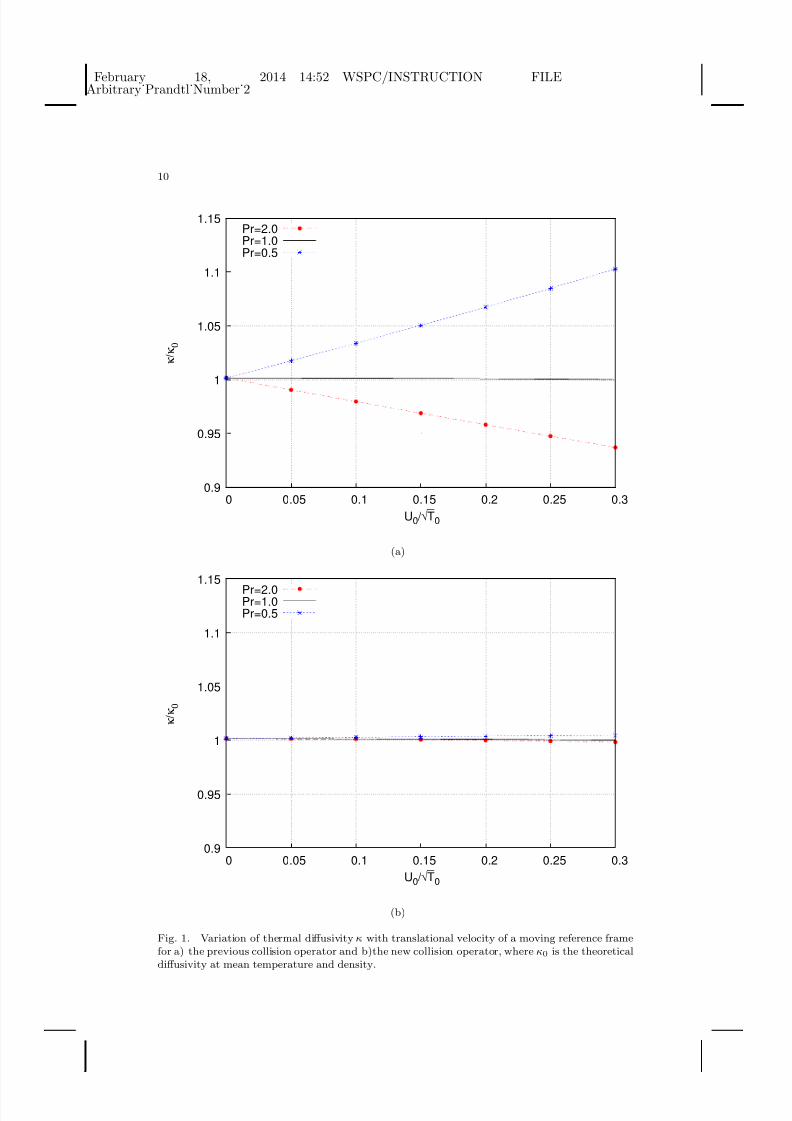
3.2. Numerical Verification

The new theoretical formulation addresses thermal fluid flows in general. But in or-

der to demonstrate the consequence, we have performed a numerical simulation of

representative case in the linearized hydrodynamic regime using a two-dimensional37 speed lattice model8, corresponding to a ninth-order accurate Gauss-Hermite

Quadrature. We have employed fourth order Hermite expansion of Maxwellian dis-

tribution for equilibrium13,8 for accurate thermohydrodynamic representation. We

perform a simple flow simulation with the following initial conditions,

ux = 0

uy = U 0 + δU 0sin(nx)

T = T 0 + δT 0sin(nx)

ρ = ρ0 [1 − (δT 0/T 0)sin(nx)] ; n = 2π/Lx (23)

A sinusoidal perturbation is given to the temperature on top of the lattice tem-

perature T 0 = 0.697953322019683, which satisfies the isotropy condition given byeqn.(6). An inverse perturbation is given to the density to maintain the pressure

(ρT ) approximately constant to avoid any acoustic modes. In order to exemplify the

difference between the two collision models, we introduce a translational velocity

U 0 (constant in space and time) to mimic a flow in a moving reference frame. A

velocity shear is also added, which will result in non-zero momentum flux tensor Π .

The amplitude of the perturbations are kept at δT 0 = 0.001, and δU 0 = 0.001. The

mean density ρ0 is kept at one. All simulations are carried out in one dimensional

grid, Lx = 100, Ly = 1, as there are no variations along the y-axis. Under such

an initial condition the temperature diffusion of the perturbation follows a simple

exponential decay,

T (t) = T 0 + δT 0e−κ0n2

t; (24)

where κ0 is the thermal diffusivity at mean temperature and density,

κ0 = k

ρ0c p=

τ k − 1

2

T 0

Obviously, such a decay rate for a Galilean invariant model should be independent

of the translational velocity value U 0.

The simulations are carried out for different Prandtl numbers and transla-

tional velocity values for both previous collision model8, eqn.(12), and current




9

collision model eqn.(21). For convenience, a small fixed viscosity value, µ =

0.00697953322019683, corresponding to τ µ = 0.51 is used for all the simulations.

Different thermal diffusivity values are chosen to get the Prandtl number values

ranging from 0.5 to 2.0. Figure 1 shows the ratio of the resulting thermal diffusiv-

ity from the simulation to the theoretical diffusivity κ0, for different translational

velocity values. One can see that the previous collision model exhibits an apparent

non-Galilean invariant behavior in thermal diffusivity at non-unity Prandtl num-

bers, while the new model largely removes this error. We have verified that the

remaining error is in part related to a lack of isotropy in the lattice velocity set

higher than ninth order quadrature.

4. Discussion

In this paper, we present a theoretical framework for formulating lattice Boltzmann

models resulting in the correct thermohydrodynamic equations with an arbitrary

Prandtl number. Unlike the previous approaches, lattice Boltzmann models derived

under the new framework do not suffer from the well-known non-Galilean invariant

artifact when Prandtl number is not unity. The critical difference of the present

approach from previous ones is that the collision operator complies with a set of

fundamental conditions pertaining to thermohydrodynamic fluxes (eqn.(18)) in the

relative reference frame. A new explicit form of the collision operator is expressed

that is generally applicable for a class of lattice Boltzmann velocity types. The

latter are those that sufficiently meet the generic set of moment isotropy conditions,eqn.(6). It is important to point out that the non-Galilean invariance problem is

not only a symptom of the specific Hermite expansion based formulations (e.g.,

eqn.(11) or eqn.(12)). Except BGK, this problem has been prevalent among most

lattice Boltzmann models having multiple relaxation times in their collision process.

The use of moments in the relative reference frame was previously proposed for

formulating certain isothermal “MRT” type of LBM models25,26. Recovery of correct

thermohydrodynamics at arbitrary Prandtl numbers has not been met in previous

LBM models.

A few fronts in thermohydrodynamics may be expanded to beyond the current

framework of collision operator representation. First of all, some potential energy

or internal degrees of freedom may be incorporated so that the specific heat val-

ues are not restricted to the dimensions of lattices used2,27. Care must be taken,

however, in order to ensure the Galilean invariance via a proper Hermite expansion

remains to be preserved (see a related discussion in the paragraph below). Another

extension is pertaining to boundary conditions, to ensure consistency with a thermo-

hydrodynamic system with non-unity Prandtl numbers. Indeed, a (soild) boundary

should also bear a Prandtl number effect in its thermodynamics (equilibrium and

non-equilibrium) as well as the boundary momentum and heat fluxes. On the other

hand, unlike collisions in a fluid flow domain, the issue of a relative reference frame

may not arise if the boundary is stationary (i.e., u = 0 at wall), and it may also




10

0.9

0.95

1

1.05

1.1

1.15

0 0.05 0.1 0.15 0.2 0.25 0.3

κ / κ 0

U0 / √ T

0

Pr=2.0

Pr=1.0

Pr=0.5

(a)

0.9

0.95

1

1.05

1.1

1.15

0 0.05 0.1 0.15 0.2 0.25 0.3

κ / κ 0

U0 / √ T

0

Pr=2.0Pr=1.0

Pr=0.5

(b)

Fig. 1. Variation of thermal diffusivity κ with translational velocity of a moving reference framefor a) the previous collision operator and b)the new collision operator, where κ0 is the theoreticaldiffusivity at mean temperature and density.




11

seem straightforward conceptually (albeit pontentially algebraically involved) for

a moving boundary with a prescribed velocity. Another important point that de-

serves further investigations in the future: The current framework only addresses the

Prandtl number related Galilean invariance issue associated with the pre-existing

inadequate formulation of collision operators8. With the new collision operator form,

the correct full thermohydrodynamic equations are analytically shown to be recov-

ered as long as a sufficient order isotropy (quadrature) (of ninth order or higher) is

applied (see Appendix). Unfortunately, though significantly reduced, the Galilean

invariance artifact is still conspicuously observed numerically at finite translational

velocity values in the resulting thermal diffusivity at non-unity Prandtl numbers,

via the thermal decay test case in the previous section. Though simple, it needs to

be said that that the thermal decay problem is known to be far more non-trivial

and delicate than that for a transverse shear fluid velocity11. Nonetheless, such an

observed small residual error (∼ 0.1%) in thermal diffusivity in our numerical tests

requires more understanding in the future. One reason we know is that the higher

order Hermite polynomials and lattice isotropy beyound those for deriving the ther-

mal diffusion term are exhibiting an higher impact at non-unity Prandtl numbers.

This has been directly verified by either reducing or increasing quadrature orders

in a lattice velocity set used in the test. On the other hand, one needs to find the

theoretical origin of such an increased sensitivity at non-unity Prandtl numbers.

Borrowing from the notion of gauge transformation, one may notice that the

explicit collision operator form eqn.(21) presented in the preceding section is not

unique for satisfying the set of conditions eqns.(17)-(18). For instance, more termsof higher order Hermite tensors may be added, similar to terms in eqn.(11) but not

in eqn.(12). Obviously, due to the orthogonality property of Hermite tensor polyno-

mials, additional terms corresponding to higher order Hermite tensor polynomials

will not alter the results for the lower order ones13,8. In particular, adding terms

with Hermite tensor polynomials of order higher than 3 to the collision expression

eqn.(21) will not change its property in regard to the conditions eqns.(17)-(18).

Furthermore, such a systematic procedure of adding terms of higher order Hermite

tensor polynomials can also be used to extend the conditions of eqns.(17)-(18) be-

yond the second and the third order moments. The key realization in formulating a

collision operator via the Hermite expansion framework is to relax the parity con-

straints between each Hermite basis function and its coefficient, so that the latter

includes not only the moment of its own Hermite function but also appropriate mo-

ments from the lower order Hermite functions, as a result of particle velocity in the

relative reference frame. Collision operators satisfying an extended set of moment

conditions may be relevant for fluid flows in broader regimes including complex and

non-Newtonian fluid physics.




12

Appendix A. Deriving Thermohydrodynamic Equations

To demonstrate that the new fundamental conditions eqns.(17) - (18) (or eqn.(20))

give rise to the correct thermohydrodynamic equations with a variable Prandtl

number, we give a brief derivation below.

Expanding eqn.(1) in Taylor series in powers of spatial and time derivatives and

neglecting terms beyond the 2nd order, we have

[∂ t + ci · ∇ + 1

2(∂ t + ci · ∇)2]f i(x, t) ≈ Ωi(x, t) (A.1)

We then apply the standard multiple scale expansion procedure for time and spatial

scales as well as for the distribution function24,18,

∂ t = ∂ t0 + 2∂ t1 , ∇ = ∇f i = f eqi + f (1)i + 2f (2)i + · · · (A.2)

where denotes a small parameter. The higher order parts of the distribution func-

tion (f (n), n ≥ 1) represent deviations from local equilibrium of various degrees,

and having vanishing contributions to the conserved quantities,i

χif (n)i = 0 , n ≥ 1 (A.3)

with χi = 1, ci, or ei. Separating terms according to powers of , so the following

set of hierarchical relations results

Ωi(f eq, x, t) = 0

(∂ t0 + ci · ∇)f eqi =j

M ijf (1)j

∂ t1f eqi + 1

2(∂ t0 + ci · ∇)2f eqi + (∂ t0 + ci · ∇)f

(1)i =

j

M ijf (2)j (A.4)

The first equation in eqn.(A.4) above is trivially satisfied with a matrix opera-

tor representation. We can then take summations of the conserved moments χi.

In particular, from the second equation in eqn.(A.4) and applying the eigen-value

relations, eqn.(20), we get

i

cicif (1)i = − τ µ

icici(∂ t0 + ci · ∇)f

eqi

i

eicif (1)i = − τ k

i

eici(∂ t0 + ci · ∇)f eqi

+ (τ k − τ µ)i

cici(∂ t0 + ci · ∇)f eqi (A.5)

Notice the term proportional to (τ k − τ µ) in the second equation above would be

missing if the absolute reference frame based collision form, eqn.(11), or the eigen-

value relations eqn.(9), were used instead.




13

After recombining terms of all orders, we get the overall set of equations for the

conserved moments,

∂ tρ + ∇ · (ρu) = 0

∂ t(ρu) + ∇ · [Π(0) + Π(1)] = 0

∂ t(ρ[D

2 T +

1

2u2]) + ∇ · [q(0) + q(1)] = 0 (A.6)

where the momentum and energy fluxes of different orders are dependent solely on

the equilibrium distribution function,

Π(0) ≡i cicif eqi

q(0) ≡i

eicif eqi

Π(1) ≡ −(τ µ − 1

2)i

cici(∂ t0 + ci · ∇)f eqi

q(1) ≡ −(τ k − 1

2)i

eici(∂ t0 + ci · ∇)f eqi

+(1 − τ k − 12

τ µ − 12

)u · Π(1) (A.7)

Once again, the term proportional to u ·Π(1) in the resulting q(1) expression above

would be missing if an absolute reference frame based formulation were used.The remaining derivations on

i cici(∂ t0 +ci ·∇)f eqi and

i eici(∂ t0 +ci ·∇)f eqi

are straightforward, since they no longer rely on properties of a collision operator

and only depend on the form of the equilibrium distribution and its spatial and time

derivatives (in the leading order). Using the 4th order form, eqn.(4), for f eqi (x, t)

and applying the generic lattice isotropy conditions, eqn.(6), up to N = 4, we obtaini

cici(∂ t0 + ci · ∇)f eqi = ρT [2Λ − 2

DI∇ · u]

i

eici(∂ t0 + ci · ∇)f eqi = D + 2

2 ρT ∇T + u · ρT [2Λ − 2

DI∇ · u] (A.8)

where the 2nd rank tensor Λ in a component form is Λαβ ≡ 12 [∂ αuβ + ∂ βuα] being

the rate of strain tensor. Combining all the results above, we arrive at the final

forms for the hydrodynamic fluxes,

Π(0) = ρuu + ρT I

q(0) = D + 2

2 ρT u +

1

2ρu2u

Π(1) = −µ[2Λ − 2

DI∇ · u]

q(1) = −k∇T + u ·Π(1) (A.9)




14

with µ ≡ (τ µ − 12

)ρT and k ≡ (τ k − 12

)D+22

ρT being the resulting viscosity and

thermal conductivity, respectively. Eqns.(A.9) are the same as that of the thermo-

hydrodynamics of a Newtonian physical fluid. It is worthwhile to verify that collision

operators such as eqn.(11) obeying eqn.(9) would lead to an incorrect form for the

non-equilibrium energy flux below,

q(1) = −k∇T + 1

P ru · Π(1) (A.10)

As a consequence, it would result in a wrong temperature equation with an addi-

tional spurious non-Galilean invariant term proportional to (1 − 1Pr

).

References

1. R. Benzi, S. Succi, and M. Vergassola, The lattice Boltzmann equation: theory and

applications , Phys. Rep. 222, 145-197 (1992).2. S. Chen and G. Doolen, Lattice Boltzmann method for fluid flows , Annu. Rev. Fluid

Mech. 30, 329-364 (1998).3. P. Bhatnagar, E. Gross, and M. Krook, A model for collision processes in gases. I.

Small amplitude processes in charged and neutral one-component systems , Phys. Rev.94 (3), 511 (1954).

4. S. Chen, H. Chen, D. Martinez, and W. Matthaeus, Lattice Boltzmann model for sim-

ulation of magnetohydrodynamics , Phys. Rev. Lett. 67, 3776-3779 (1991).5. H. Chen, S. Chen, and W. Matthaeus, Recovery of the Navier-Stokes equations using

a lattice-gas Boltzmann method , Phys.Rev. A 45, 5339-5342 (1992).6. Y. Qian, D. D’Humieres, and P. Lallemand, Lattice BGK models for Navier-Stokes

equation , Europhys. Lett. 17, 479-484 (1992).7. H. Chen, C. Teixeira, and K. Molvig, Digital physics approach to computational fluid

dynamics: Some basic theoretical features , Intl. J. Mod. Phys. C 9 (8), 675 (1997).8. X. Shan, and H. Chen, A general multiple-relaxation-time Boltzmann collision model ,

International Journal of Modern Physics C 18, 635 (2007).9. C. Thantanapally, S. Singh, S. Succi, and S. Ansumali, Quasiequilibrium lattice Boltz-

mann models with tunable Prandtl number for incompressible hydrodynamics , Interna-tional Journal of Modern Physics C 24 (12), 1340004 (2013).

10. F. Higuera, S. Succi, and R. Benzi, Lattice gas dynamics with enhanced collisions ,Europhys. Lett. 9, 345 (1989).

11. K. Huang, “Statistical Mechanics”, 2nd edn., John Wiley (1987).12. X. Shan, and X. He, Discretization of the velocity space in the solution of the Boltz-

mann equation , Phys. Rev. Lett. 80, 65 (1998).

13. X. Shan, X. Yuan, and H. Chen, Kinetic theory representation of hydrodynamics: a way beyond the Navier-Stokes equation , J. Fluid Mech. Vol 550, 413, (2006).

14. X.B. Nie, X. Shan, and H. Chen, Galilean invariance of lattice Boltzmann models ,Europhysics Letters Vol 81, 34005, (2008).

15. R. Zhang, H. Chen, and X. Shan, Efficient kinetic method for fluid simulation beyond

the Navier-Stokes equation , Physical Rew. E 74, 046703 (2006).16. H. Grad, Note on N-dimensional hermite polynomials , Commun. Pure Appl. Math. 2,

325 (1949); and H. Grad, On the kinetic theory of rarefied gases , Commun. Pure Appl.Math. 2, 331 (1949).

17. H. Grad, The profile of a steady plane shock wave , Commun. Pure Appl. Math. 5, 257(1952).




15

18. U. Frisch, D. D’Humieres, B. Hasslacher, P. Lallemand, Y. Pomeau, and J.P. Rivet,Lattice gas hydrodynamics in two and three dimensions , Complex Systems 1, 649-707(1987).

19. H. Chen and S. Orszag, Moment isotropy and discrete rotational symmetry of two-

dimensional lattice vectors , Philosophical Transactions of The Royal Society A 369

(1944), 2176-2183 (2011).20. H. Chen and X. Shan, Fundamental conditions for N-th-order accurate lattice Boltz-

mann models , Physica D 237, issues: 14-17, 2003-2008 (2007).21. H. Chen, I. Goldhirsch, and S. A. Orszag, Discrete Rotational Symmetry, Moment

Isotropy, and Higher Order Lattice Boltzmann Models , Journal of Sci. comp. 34, 87-112(2008).

22. H. Chen, R. Zhang, I. Staroselsky, and M. Jhon, Recovery of full rotational invariance

in lattice Boltzmann formulations for high Knudsen number flows , Physica A 362, 125-131 (2006).

23. J. Latt and B. Chopard, Lattice Boltzmann method with regularized pre-collision dis-

tribution functions , Math. Comput. Simulat. 72(2-6), 165 (2006).24. S. Chapman and T. Cowling, “The Mathematical Theory of Non-Uniform Gases”, 3rd

edn., Cambridge Univ. Press, Cambridge (1990).25. M. Geier, A. Greiner, and J. G. Korvink, Cascaded digital lattice Boltzmann automata

for high Reynolds number flow , Physical Review E 73,66705 (2006).26. P. Asinari, Generalized local equilibrium in the cascaded lattice Boltzmann method ,

Physical Review E 78,016701 (2008).27. X. Nie, X. Shan, and H. Chen, Thermal lattice Boltzmann model for gases with internal

degrees of freedom , Phys. Rev. E 77, 035701(R), (2008).

recovery of galilean invariance in thermal lattice boltzmann models

Documents