Reinforcement Learning Applied to Forex Trading

João Maria Branco Carapuço

Thesis to obtain the Master of Science Degree in

Engineering Physics

Supervisor(s): Prof. Rui Fuentecilla Maia Ferreira NevesProf. Maria Teresa Haderer de la Peña Stadler

Examination Committee

Chairperson: Prof. Maria Joana Patrício Gonçalves de SáSupervisor: Prof. Rui Fuentecilla Maia Ferreira Neves

Member of the Committee: Prof. Rui Manuel Agostinho Dilão

November 2017

ii

To my mother Cristina.

Without her life would be much darker.

iii

iv

Acknowledgments

I would like to thank my supervisor, professor Rui Neves, for his patience and dedication. All the best for

future friday afternoon meetings and new students!

A word of appreciation for all my family, truly a part of my life that has been most fortunate. In

particular: my grandparents Antonio, Zizi, Nini and Lu, all are truly important to me and fill me with

wonderful memories, my sister Maria, the day she was born I received presents and missed school and

although the following 19 years haven’t been nearly as good, I still love her, my mother Tita, to whom I

dedicate this thesis, a small drop in the ocean of love and support that I still have to pay back, and last

but certainly not least my father Antonio, whose company has taught me so much and who I will always

look up to.

Finally, I would like to mention those friends that were more present during this phase of my life:

Antonio Ornelas, always my MEFT comrade, Teresa, Ricardo and Bernardo, awesome company, any-

where, anytime, Galileu, consistently terrible company, Claudio and Nones, always make me smile and

laugh, Yanne, hour-long conversations that go by in five minutes.

v

vi

Resumo

Nesta tese e descrita a implementacao de um sistema que efectua transaccoes automaticas no mer-

cado de moeda com o intuito lucrar com flutuacoes de cotacao com aprendizagem por reforco e redes

neuronais.

O funcionamento de um sistema de aprendizagem por reforco pode ser resumido em tres sinais: uma

representacao do estado do ambiente dada ao sistema, a accao que este toma nesse estado e uma

recompensa por essa accao. Uma rede neuronal e composta por neuronios artificiais interconectados

que apesar de simples, como um todo estabelecem uma relacao complexa e nao-linear entre entradas

e saıdas. Essa relacao pode ser ajustada para diferentes fins num processo de treino com aprendiza-

gem automatica.

O sistema transaccional concebido consiste numa rede neuronal com tres camadas ocultas de 20

neuronios ReLU cada e uma camada de output com 3 neuronios lineares, treinada para funcionar

sob o paradigma de aprendizagem por reforco. A rede recebe o estado do mercado, composto por

caracterısticas extraıdas do historico de precos e volumes, e da como saıda o valor Q de cada accao

possıvel nesse estado. Valor Q e uma estimativa, construıda no processo de treino, das recompensas

que uma accao num dado estado vai acumular no futuro. A escolha da accao com melhor valor Q leva

ao maior lucro futuro quando os valores estimados de Q tem qualidade.

No mercado EUR/USD desde 2010 a 2017 este sistema obteve em 10 testes com diferentes condicoes

iniciais um lucro total medio de 114.0±19.6%, ou seja, uma media de 16.3±2.8% por ano.

Palavras-chave: Aprendizagem de maquina, Redes neuronais, Aprendizagem por reforco,

Q-learning, Mercado de moeda

vii

viii

Abstract

This thesis describes the implementation of a system that automatically trades in the foreign exchange

market to profit from price fluctuations with reinforcement learning and neural networks.

A reinforcement learning system can be summed up by three signals: a representation of the environ-

ment’s state given to the system, the action it chooses for that state and a reward for the chosen action.

A neural network is a group of interconnected artificial neurons, which albeit individually very simple, as

a whole establish a complex non-linear relationship between input and output. This relationship can be

molded through an automatic training process.

The trading system described in this thesis is a neural network with three hidden layers of 20 ReLU

neurons each and an output layer of 3 linear neurons, trained to work under the reinforcement learning

paradigm, more precisely, under the Q-learning algorithm. This network receives as input a state signal

from the market environment, comprised of features extracted from the history of prices and volumes,

and outputs the Q-value of each action available for that state. Q-value is an estimate, built during the

training process, of the amount of reward an action performed in a given state may accumulate in the

future. Choosing the action with the best Q value leads to the largest future profit when Q-value estima-

tes are accurate.

In the EUR/USD market from 2010 to 2017 the system yielded, over 10 tests with varying initial conditi-

ons, an average total profit of 114.0±19.6%, an yearly average of 16.3±2.8%.

Keywords: Machine learning, Neural networks, Reinforcement learning, Q-learning, Foreign

exchange market

ix

x

Contents

Acknowledgments . . . . . . . . . . . . . . . . . . . . . . . . . . . . . . . . . . . . . . . . . . . v

Resumo . . . . . . . . . . . . . . . . . . . . . . . . . . . . . . . . . . . . . . . . . . . . . . . . . vii

Abstract . . . . . . . . . . . . . . . . . . . . . . . . . . . . . . . . . . . . . . . . . . . . . . . . . ix

List of Tables . . . . . . . . . . . . . . . . . . . . . . . . . . . . . . . . . . . . . . . . . . . . . . xiii

List of Figures . . . . . . . . . . . . . . . . . . . . . . . . . . . . . . . . . . . . . . . . . . . . . xv

Nomenclature . . . . . . . . . . . . . . . . . . . . . . . . . . . . . . . . . . . . . . . . . . . . . . xix

Glossary . . . . . . . . . . . . . . . . . . . . . . . . . . . . . . . . . . . . . . . . . . . . . . . . xxiii

1 Introduction 1

1.1 Foreign Exchange Market . . . . . . . . . . . . . . . . . . . . . . . . . . . . . . . . . . . . 2

1.2 Machine Learning . . . . . . . . . . . . . . . . . . . . . . . . . . . . . . . . . . . . . . . . 4

1.3 Objectives . . . . . . . . . . . . . . . . . . . . . . . . . . . . . . . . . . . . . . . . . . . . . 6

1.4 Contributions . . . . . . . . . . . . . . . . . . . . . . . . . . . . . . . . . . . . . . . . . . . 6

1.5 Outline of Contents . . . . . . . . . . . . . . . . . . . . . . . . . . . . . . . . . . . . . . . . 7

2 Background 9

2.1 Financial Trading . . . . . . . . . . . . . . . . . . . . . . . . . . . . . . . . . . . . . . . . . 9

2.1.1 Technical Analysis . . . . . . . . . . . . . . . . . . . . . . . . . . . . . . . . . . . . 10

2.1.2 Positions . . . . . . . . . . . . . . . . . . . . . . . . . . . . . . . . . . . . . . . . . 12

2.2 Reinforcement Learning . . . . . . . . . . . . . . . . . . . . . . . . . . . . . . . . . . . . . 12

2.2.1 State . . . . . . . . . . . . . . . . . . . . . . . . . . . . . . . . . . . . . . . . . . . . 13

2.2.2 Reward . . . . . . . . . . . . . . . . . . . . . . . . . . . . . . . . . . . . . . . . . . 15

2.2.3 Actions . . . . . . . . . . . . . . . . . . . . . . . . . . . . . . . . . . . . . . . . . . 15

2.2.4 Q-Learning . . . . . . . . . . . . . . . . . . . . . . . . . . . . . . . . . . . . . . . . 16

2.2.5 Policy . . . . . . . . . . . . . . . . . . . . . . . . . . . . . . . . . . . . . . . . . . . 18

2.2.6 Limitations of Reinforcement Learning . . . . . . . . . . . . . . . . . . . . . . . . . 19

2.3 Neural Networks . . . . . . . . . . . . . . . . . . . . . . . . . . . . . . . . . . . . . . . . . 20

2.3.1 Neurons . . . . . . . . . . . . . . . . . . . . . . . . . . . . . . . . . . . . . . . . . . 20

2.3.2 Topology . . . . . . . . . . . . . . . . . . . . . . . . . . . . . . . . . . . . . . . . . 22

2.3.3 Backpropagation . . . . . . . . . . . . . . . . . . . . . . . . . . . . . . . . . . . . . 23

2.3.4 Gradient Descent . . . . . . . . . . . . . . . . . . . . . . . . . . . . . . . . . . . . . 26

xi

2.3.5 Deep Networks . . . . . . . . . . . . . . . . . . . . . . . . . . . . . . . . . . . . . . 27

2.4 Related Work . . . . . . . . . . . . . . . . . . . . . . . . . . . . . . . . . . . . . . . . . . . 29

3 Implementation 33

3.1 Overview . . . . . . . . . . . . . . . . . . . . . . . . . . . . . . . . . . . . . . . . . . . . . 33

3.2 Preprocessing . . . . . . . . . . . . . . . . . . . . . . . . . . . . . . . . . . . . . . . . . . 35

3.2.1 Feature Extraction . . . . . . . . . . . . . . . . . . . . . . . . . . . . . . . . . . . . 37

3.2.2 Standardization . . . . . . . . . . . . . . . . . . . . . . . . . . . . . . . . . . . . . . 41

3.3 Market Simulation . . . . . . . . . . . . . . . . . . . . . . . . . . . . . . . . . . . . . . . . 43

3.3.1 time skip and nr paths . . . . . . . . . . . . . . . . . . . . . . . . . . . . . . . . . . 44

3.3.2 Reward Signal . . . . . . . . . . . . . . . . . . . . . . . . . . . . . . . . . . . . . . 46

3.3.3 State Signal . . . . . . . . . . . . . . . . . . . . . . . . . . . . . . . . . . . . . . . . 48

3.3.4 Training Procedure . . . . . . . . . . . . . . . . . . . . . . . . . . . . . . . . . . . . 50

3.3.5 Example . . . . . . . . . . . . . . . . . . . . . . . . . . . . . . . . . . . . . . . . . . 52

3.4 Q-Network . . . . . . . . . . . . . . . . . . . . . . . . . . . . . . . . . . . . . . . . . . . . 54

3.4.1 Learning Function . . . . . . . . . . . . . . . . . . . . . . . . . . . . . . . . . . . . 56

3.5 Hyper-parameter Selection . . . . . . . . . . . . . . . . . . . . . . . . . . . . . . . . . . . 58

4 Testing 63

4.1 5,000 time skip . . . . . . . . . . . . . . . . . . . . . . . . . . . . . . . . . . . . . . . . . . 64

4.1.1 Results . . . . . . . . . . . . . . . . . . . . . . . . . . . . . . . . . . . . . . . . . . 64

4.1.2 Result Analysis . . . . . . . . . . . . . . . . . . . . . . . . . . . . . . . . . . . . . . 70

4.2 10,000 time skip . . . . . . . . . . . . . . . . . . . . . . . . . . . . . . . . . . . . . . . . . 73

4.2.1 Results . . . . . . . . . . . . . . . . . . . . . . . . . . . . . . . . . . . . . . . . . . 73

4.2.2 Result Analysis . . . . . . . . . . . . . . . . . . . . . . . . . . . . . . . . . . . . . . 77

5 Conclusions 81

5.1 Future Work . . . . . . . . . . . . . . . . . . . . . . . . . . . . . . . . . . . . . . . . . . . . 82

Bibliography 85

A Learning curves 89

xii

List of Tables

1.1 Trade volume for the three most traded currency pairs. Daily averages for the month of

April, in billions of US dollars and percentage of total volume. Note that over the past

decade the EUR/USD pair has accounted for almost a quarter of total foreign exchange

daily volume. [2] . . . . . . . . . . . . . . . . . . . . . . . . . . . . . . . . . . . . . . . . . 4

2.1 Excerpt of tick data for the EUR/USD currency pair with the Duskacopy broker. Volume is

in millions of units traded. . . . . . . . . . . . . . . . . . . . . . . . . . . . . . . . . . . . . 10

2.2 Summary of performance obtained by RL trading systems tested on the foreign exchange

market. . . . . . . . . . . . . . . . . . . . . . . . . . . . . . . . . . . . . . . . . . . . . . . 29

3.1 Interpretation of each action signal an. . . . . . . . . . . . . . . . . . . . . . . . . . . . . . 34

3.2 The three datasets used for hyper-parameter selection. . . . . . . . . . . . . . . . . . . . 58

3.3 Hyper-parameters chosen for the trading system. . . . . . . . . . . . . . . . . . . . . . . . 59

4.1 A description of the test datasets. Each one is referred to by year followed by quadrimester. 66

4.2 Overview of the test results for time skip = 5000. . . . . . . . . . . . . . . . . . . . . . . . 67

4.3 Simple and compounded total test profit for time skip = 5000. . . . . . . . . . . . . . . . . 68

4.4 Trade-by-trade analysis for time skip = 5000. Note that trades from all 10 paths are

included. Duration is in number of ticks. . . . . . . . . . . . . . . . . . . . . . . . . . . . . 68

4.5 Comparison between validation and test results for time skip = 5000. . . . . . . . . . . . 70

4.6 Simple yearly profit and maximum drawdown for time skip = 5000. . . . . . . . . . . . . . 71

4.7 Overview of the testing procedure results for time skip = 10000. . . . . . . . . . . . . . . 75

4.8 Simple and compounded total test profit for time skip = 10000. . . . . . . . . . . . . . . . 77

4.9 Trade-by-trade analysis for time skip = 10000. Note that trades from all 20 paths are

included. Duration is the number of ticks during which a position was kept open. . . . . . 77

4.10 Comparison between validation and test results. . . . . . . . . . . . . . . . . . . . . . . . 78

4.11 Simple and compounded total test profit for a mix of 5,000 and 10,000 time skip. . . . . . 80

xiii

xiv

List of Figures

1.1 50-day moving averages of the percent of total volume with at least one algorithmic coun-

terparty, for three of the most commonly traded currencies. [1] . . . . . . . . . . . . . . . 2

1.2 Price quotes from the swiss broker Duskacopy. Green means price has gone up since the

last value, and red means it has gone down. Traditionally price quotes had five significant

figures of which the last digit was known as a pip, the smallest possible price change at

the time. Recently some brokers added one more digit of precision, known as fractional

pip, which is shown here in a smaller font in reference to the traditional pip. The spread,

the number in the small white box between the Bid and Ask prices, is also typically given

in units of pips. . . . . . . . . . . . . . . . . . . . . . . . . . . . . . . . . . . . . . . . . . . 3

1.3 Performance of Deepmind reinforcement learning system on various Atari games. Per-

formance is normalized with respect to a professional human games tester (100%) and

random play (0%): 100 ·(score− random play score)/(human score− random play score).

Error bars indicate standard deviation across 30 evaluation episodes, starting with diffe-

rent initial conditions. [6] . . . . . . . . . . . . . . . . . . . . . . . . . . . . . . . . . . . . . 5

2.1 The RL learning framework. [21] . . . . . . . . . . . . . . . . . . . . . . . . . . . . . . . . 13

2.2 A very simplified drawing of a biological neuron (left) and its mathematical model (right).

[26] . . . . . . . . . . . . . . . . . . . . . . . . . . . . . . . . . . . . . . . . . . . . . . . . 21

2.3 Example of feedforward and recurrent neural networks with one hidden layer. [28] (modified) 22

2.4 A fully-connected feed-forward neural network with two hidden layers and no skip con-

nections. [29] (modified) . . . . . . . . . . . . . . . . . . . . . . . . . . . . . . . . . . . . . 23

2.5 Binary classification using a shallow model with 20 hidden units (solid line) and a deep

model with two layers of 10 units each (dashed line). The right panel shows a close-up

of the left panel. Filled markers indicate errors made by the shallow model. The learnt

decision boundary illustrates the advantage of depth, it captures the desired boundary

more accurately, approximating it with a larger number of linear pieces. [39] . . . . . . . . 28

2.6 Adaptive reinforcement learning (ARL). [43] . . . . . . . . . . . . . . . . . . . . . . . . . . 30

2.7 Multiagent Q-learning. [46] . . . . . . . . . . . . . . . . . . . . . . . . . . . . . . . . . . . 31

3.1 Flow of information between the three main components of the system: preprocessing

stage, market simulation and Q-network. . . . . . . . . . . . . . . . . . . . . . . . . . . . . 35

xv

3.2 400,000 ticks (2013.01.02 - 2013.01.09) of EUR/USD pair market data from Duskacopy

broker: (a) bid and ask price values (b) bid and ask volume in millions of units. . . . . . . 36

3.3 Bid-Ask spread for the first 100,000 ticks of the data segment from 3.2. Spread varies

between a few well defined levels reflecting the broker’s assessment of market conditions. 38

3.4 Generalization to section B from the training data in section A is difficult because the

model has not been trained with inputs in the range covered by section B. [49] . . . . . . 39

3.5 Features extracted from the same segment of data as Figure 3.3, divided into 500-tick

windows. (a) shows the original features and (b) depicts our solution to the non-stationarity. 40

3.6 Distribution of the unstandardized feature variables extracted from 500 tick windows from

roughly one year of bid (red), bid volume (green), ask volume (cyan) and spread (blue)

data. X-axis of each distribution is bounded to the maximum and minimum value, so all

values depicted have at least one occurrence even if not visible on the Y-axis due to scale.

Raw data from the EUR/USD pair during 2013 from Duskacopy broker. . . . . . . . . . . 42

3.7 Distribution of feature variables, extracted from the same raw data as Figure 3.6, filtered,

with q = 99, and standardized. Bid (red), bid volume (green), ask volume (cyan) and

spread (blue) data. . . . . . . . . . . . . . . . . . . . . . . . . . . . . . . . . . . . . . . . . 43

3.8 Schematic of a dataset of ticks and how the market environment sequentially visits those

ticks through two different paths, in orange and black. Top: time skip = 2, Bottom:

time skip = 4. These paths would be very similar, but for larger values of time skip

the distance between ticks visited in different paths increases and so does the quality of

information added by having different paths. . . . . . . . . . . . . . . . . . . . . . . . . . . 45

3.9 Example of learning curves with and without the nr paths dynamic. Training dataset:

01/2011 to 01/2012. Validation dataset: 01/2012 to 07/2012. How these learning curves

are produced is further explained in subsection 3.3.4. . . . . . . . . . . . . . . . . . . . . 46

3.10 Behaviour with the initial reward approach on a 6 month validation dataset from 2012.01

to 2012.06. Each step skips 5000 ticks. Green arrows are long positions and red arrows

are short positions. . . . . . . . . . . . . . . . . . . . . . . . . . . . . . . . . . . . . . . . . 46

3.11 Example of behaviour with the final approach to reward on a 6 month validation dataset

from 2012.01 to 2012.06. Each step skips 5000 ticks. Green arrows are long positions

and red arrows are short positions. . . . . . . . . . . . . . . . . . . . . . . . . . . . . . . . 47

3.12 Distribution of possible returns in a EUR/USD Duskacopy dataset of the year 2013, with

time skip = 500. . . . . . . . . . . . . . . . . . . . . . . . . . . . . . . . . . . . . . . . . . 48

3.13 Training Procedure. . . . . . . . . . . . . . . . . . . . . . . . . . . . . . . . . . . . . . . . . 51

3.14 Schematic of the trading system’s Q-network. sn is the nth element of the vector re-

presenting the state s. Hidden and output neurons have ReLU and Linear activations

respectively. . . . . . . . . . . . . . . . . . . . . . . . . . . . . . . . . . . . . . . . . . . . . 55

3.15 Learning curves for dataset A (top), B (middle) and C (bottom) with position size = 10000. 60

xvi

4.1 Rolling window approach to testing. Note that the training set includes both training da-

taset and validation dataset, while the test set is where the final model obtained with the

training procedure is applied to assess its ”true” performance. [49] . . . . . . . . . . . . . 64

4.2 Learning curves for time skip = 5000. Red circle marks the chosen model. Remaining

learning curves were placed in Appendix A. . . . . . . . . . . . . . . . . . . . . . . . . . . 65

4.3 Learning curves for the 2011 p.3 test using the standard 24/6 months training/validation. . 66

4.4 A Q-network’s learning curve from the original Atari playing system on ’Seaquest’. [8] . . 67

4.5 System behaviour from 2011 p.1 (top), 2015p.3 (middle) and 2016 p.3 (bottom). Green

and red arrows represent Long and Short positions respectively. Each step is 5,000 ticks

apart. . . . . . . . . . . . . . . . . . . . . . . . . . . . . . . . . . . . . . . . . . . . . . . . 69

4.6 Bid prices for EUR/USD pair (top) and equity growth curve with and without compoun-

ding (bottom) for time skip = 5000. Light area around equity curves represents their

uncertainty. X-axis is in units of ticks. . . . . . . . . . . . . . . . . . . . . . . . . . . . . . . 72

4.7 Average drawdowns for time skip = 5000, uncertainty was not included for clarity. X-axis

is in units of ticks. . . . . . . . . . . . . . . . . . . . . . . . . . . . . . . . . . . . . . . . . . 72

4.8 Learning curves for time skip = 10000. Red circle marks the chosen model. Remaining

learning curves were placed in Appendix A, as appendix. . . . . . . . . . . . . . . . . . . 74

4.9 System behaviour from 2011 p.1 (top), 2015p.3 (middle) and 2016 p.3 (bottom). Green

and red arrows represent Long and Short positions respectively. Each step is 10,000 ticks

apart. . . . . . . . . . . . . . . . . . . . . . . . . . . . . . . . . . . . . . . . . . . . . . . . 76

4.10 Bid prices for EUR/USD pair (top) and equity growth curve with and without compoun-

ding (bottom) for time skip = 10000. Light area around equity curves represents their

uncertainty. X-axis is in units of ticks. . . . . . . . . . . . . . . . . . . . . . . . . . . . . . . 79

4.11 Average drawdowns for time skip = 10000, uncertainty was not included for clarity. X-axis

is in units of ticks. . . . . . . . . . . . . . . . . . . . . . . . . . . . . . . . . . . . . . . . . . 79

4.12 Bid prices for EUR/USD pair (top) and equity growth curve with and without compoun-

ding (bottom) for a mix of 5,000 and 10,000 time skip. Light area around equity curves

represents their uncertainty. X-axis is in units of ticks. . . . . . . . . . . . . . . . . . . . . 80

A.1 Learning curves, time skip = 5000 (cont.) Red circle marks the chosen model. . . . . . . 89

A.2 Learning curves, time skip = 5000 (cont.) Red circle marks the chosen model. . . . . . . 90

A.3 Learning curves, time skip = 5000 (cont.) Red circle marks the chosen model. . . . . . . 91

A.4 Learning curves, time skip = 10000 (cont.) Red circle marks the chosen model. . . . . . 91

A.5 Learning curves, time skip = 10000 (cont.) Red circle marks the chosen model. . . . . . 92

xvii

xviii

Nomenclature

Reinforcement Learning

γ Reinforcement learning’s discount-rate parameter.

A The set of all actions.

E[X] Expectation of random variable X.

S The set of all states.

π A policy.

π(s) Action taken in state s under deterministic policy π.

π∗ The optimal policy.

a An action.

At The action at step t.

Gt Cumulative discounted reward following step t.

p(s′, r | s, a) Probability of transition to state s′ with reward r, from state s taking action a.

Q(s, a) Array estimate of an action-value function qπ or q∗ for state s and action a.

xix

Q(s, a; θ) Function approximation estimate of an action-value function qπ or q∗ for state s and

action a with parameters θ.

q∗(s, a) Value of taking action a in state s under the optimal policy.

qπ(s, a) Value of taking action a in state s under policy π.

r A reward.

Rt Reward at step t.

s, s′ States.

St The state at step t.

vπ(s) Value of state s under policy π.

Financial

Ai The ask price from tick i in the dataset.

Bi The bid price from tick i in the dataset.

Ti The tick i in the dataset.

V ai The trading volume at the ask price from tick i in the dataset.

V bi The trading volume at the bid price from tick i in the dataset.

Neural Networks

α Learning-rate parameter.

Sk The subsample of cases for update k with mini-batch gradient descent.

xx

Wk The set of all weights in the network at iteration k.

al The vector of all activations from the lth layer.

bl The vector of all biases in the lth layer.

dp The desired output for input zp.

netl The vector of all total inputs to the lth layer.

zp The input from training case p.

alj The activation of the jth neuron in the lth layer.

blj The bias of the jth neuron in the lth layer.

E(W) Total error between desired and actual output for set of weights W.

Ep(W) Error between desired and actual output for training case p and set of weights W.

netlj The total input to the jth neuron in the lth layer.

W l The matrix containing all weights for all neurons in the lth layer.

wljk The weight the jth neuron in the lth layer gives to the part of its input that comes from

the kth neuron in the (l − 1)th layer.

xxi

xxii

Glossary

Action-value function

Measures how good it is to perform a certain action in a given state, based on expected future

reward.

Ask

In the context of Forex, it is the price at which a broker is willing to sell a unit of base currency, in

units of counter currency.

Backpropagation

A widely used procedure to obtain the error contribution from each of a neural network’s parame-

ters.

Bid

In the context of Forex, it is the price at which a broker is willing to buy a unit of base currency, in

units of counter currency.

Deep Network

A neural network with more than two non-linear layers.

Environment

That with which the RL agent interacts with.

Feedforward

The property of a neural network whose connections never form a cycle.

Forex/FX

The foreign exchange market.

Long

In the context of Forex, it is a trading position that entails buying units of the base currency while

creating debt in the counter currency.

MSE

Mean squared error.

xxiii

Policy

A mapping from states of the environment to actions to be taken when in those states.

Q-learning

An RL algorithm meant to estimate the optimal action-value function.

Q-network

A neural network designed to work under the Q-learning algorithm.

Q-value

An output of the action-value function obtained with the Q-learning algorithm.

RL

Reinforcement learning. A machine learning paradigm meant to create systems that learn from

interaction to achieve a goal.

RMSProp

Root Mean Square Propagation, a gradient descent implementation with adaptive learning rate.

ReLU

Rectified linear unit, a type of artificial neuron.

Recurrent

The property of a neural network whose connections form a cycle.

Return

The relative difference between two prices and, consequently, the relative change of unrealized

profit of an open position.

Reward

One of the input signals of a reinforcement learning system. Should relay to the system what is its

objective by providing feedback on its performance.

Short

In the context of Forex, it is a trading position that entails buying units of the counter currency while

creating debt in the base currency.

State-value function

Measures how good it is to be in a given state, based on expected future reward.

State

One of the input signals of a reinforcement learning system. Should include all relevant information

about the environment for decision making.

xxiv

Tick

The smallest granularity of foreign exchange data.

Topology

The frame of neurons and their interconnection structure in a neural network.

Unrealized Profit

The profit that a open position would provide if it was closed at this moment.

Value

In the context of RL, is the amount of reward the system is expected to accumulate in a given state.

Volume

Number of units traded at a certain price or during a certain time period.

xxv

xxvi

Chapter 1

Introduction

In order to obtain an edge over their competitors, financial institutions and other market participants

have been devoting an increasing amount of time and resources to the development of algorithmic

trading systems. Algorithmic trading refers to any form of trading using algorithms to automate all or

some part of the trade cycle, which includes pre-trade analysis, generation of the trading signal and

execution of the trading signal. For example, an algorithm focused on pre-trade analysis could output

price predictions, while an algorithm for trading signal generation would take it a step further and decide

when to open or close positions in the market and finally a trade execution algorithm would have the

ability to further optimize trading signals by deciding how large those positions should be and how to

place them in the market.

The use of algorithmic trading began in the U.S. stock market more than 20 years ago and has nowa-

days become common in major financial markets [1]. The adoption of algorithmic trading in the foreign

exchange market (Forex or FX), the market this thesis deals with, is a more recent phenomenon since

the two major trading platforms for currency only began to allow algorithmic trades in the last decade.

But it has grown extremely rapidly, and presently a majority of foreign exchange transactions involve at

least one algorithmic counterparty, as shown in Figure 1.1. Despite concerns there is no evident causal

relationship between algorithmic trading and increased market volatility. If anything, the presence of

more algorithmic trading appears to lead to lower market volatility and increases liquidity during periods

of market stress [1]. Although algorithmic trading was initially reserved for financial institutions and other

major players in the markets, an increase in the availability of information, ease of access to the market

and computational power of commercial computer technology has expanded this phenomenon to the

retail trading and academic worlds.

This thesis describes the development of an algorithmic system that generates trading signals for the

foreign exchange market using recent developments from the field of machine learning. These develop-

ments concern the use of Q-learning, an algorithm from the reinforcement learning (RL) paradigm, in

tandem with neural networks (NNs), a computational tool that mimics biological brains, to create what is

known as a Q-network. Enveloping the Q-network, the system’s core, is a simulated market environment

of our design that provides a widely applicable framework for efficient usage of market data in training

1

Figure 1.1: 50-day moving averages of the percent of total volume with at least one algorithmic counter-party, for three of the most commonly traded currencies. [1]

and testing a system for financial trading.

In this first chapter we introduce the foreign exchange market (section 1.1) followed by a concise

overview of the machine learning field focusing on the approaches used in this thesis (section 1.2). We

close the chapter by discussing the objectives and challenges of this work (section 1.3), our contributions

(section 1.4) and the layout of the rest of the thesis (section 1.5).

1.1 Foreign Exchange Market

A financial market is a broad term describing any aggregate of possible buyers and sellers of assets

and the transactions between them. Common usage of the term typically implies some characteristics

such as having transparent pricing, basic regulations on trading, costs and fees. The assets traded in

financial markets are intangible, their value is derived only from contractual claim. They can be roughly

divided into three categories, commodities, securities and currency. Commodities represent the promise

of delivery of a certain good, be it coal, gold, oranges, coffee, etc., that meets certain standards of quality

that make each of its units interchangeable, thus facilitating trade. The legal definition of securities varies

for different jurisdictions, but they can be broadly divided into debt securities, which represent borrowed

money with specific repayment parameters, and equity securities, representing partial ownership of an

entity. Stocks, usually the asset most associated with financial trading, fall into the category of equity

securities. Finally, the market that will be focused on in this thesis is that of currency, which is simply

money represented, sustained and given value by a certain central bank/government and which can be

traded by its equivalent from another nation. This is the foreign exchange market, which exists to assist

international trade and investments by enabling currency conversion.

Since currencies are the basis on which value is assigned to an asset they can only be measured in

comparison with another currency, thus all currencies are traded in pairs. Figure 1.2 shows an exam-

ple of price quotes displayed for traders in real time for four different currency pairs: EUR/JPY (Euro-

2

Japanese Yen), EUR/USD (Euro-US Dollar) pair, GBP/USD (British Pound-US Dollar) and NZD/USD

(New Zealand Dollar-US Dollar). When the price is quoted, the first currency is the base and the se-

Figure 1.2: Price quotes from the swiss broker Duskacopy. Green means price has gone up since thelast value, and red means it has gone down. Traditionally price quotes had five significant figures ofwhich the last digit was known as a pip, the smallest possible price change at the time. Recently somebrokers added one more digit of precision, known as fractional pip, which is shown here in a smaller fontin reference to the traditional pip. The spread, the number in the small white box between the Bid andAsk prices, is also typically given in units of pips.

cond is the counter. The prices are always in terms of amount of counter currency for one unit of base

currency. So the bid represents how much the broker offers in counter currency for one unit of base and

the ask is how much the broker wants in counter currency for one unit of base. Spread is the difference

between them and is always lost by the trader when he opens and then closes a position, acting as a

commission for the trade.

While stock trading is centralized in stock exchanges, meaning all orders are routed to the exchange

where a company is listed and then are matched with an offsetting order, with no other competing market,

the Forex market operates very differently. There is no one location where currencies are traded. Without

a central exchange, the trading rates are set by market makers, firms that stand ready to buy and sell

currency held in inventory, on a regular and continuous basis at a publicly quoted price. They quote both

a price a bid and an ask, hoping to make a profit on the price differential, the spread. At the highest level

these market makers are huge banks selling and buying to mostly other banks, thus being commonly

called the interbank market. Other than banks, only the largest hedge funds and large multinational

companies can directly access the interbank market as it deals only with very large orders. There is little

oversight, but fierce competition ensures fair pricing and small spreads. Retail level trading is mediated

through brokers, companies which have access to this interbank market and act as the middle man for

smaller traders. In this thesis we use historical datasets from Duskacopy, a swiss bank and broker.

The system developed in this thesis could theoretically be adapted to any financial market, but there

is a particular reason why we chose to focus on foreign exchange during its development and subsequent

testing. Forex is by far the largest financial market in terms of volume traded. According to the Bank

for International Settlements, in the 2016 Triennial Central Bank Survey [2], trading in foreign exchange

markets averaged 5.1 trillion $ per day in April 2016. To put this number into perspective, the New York

3

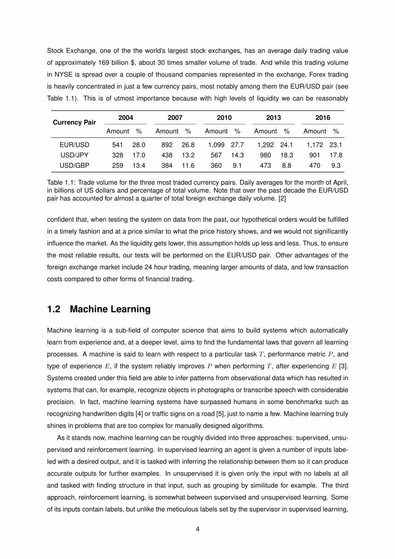
Stock Exchange, one of the the world’s largest stock exchanges, has an average daily trading value

of approximately 169 billion $, about 30 times smaller volume of trade. And while this trading volume

in NYSE is spread over a couple of thousand companies represented in the exchange, Forex trading

is heavily concentrated in just a few currency pairs, most notably among them the EUR/USD pair (see

Table 1.1). This is of utmost importance because with high levels of liquidity we can be reasonably

Currency Pair2004 2007 2010 2013 2016

Amount % Amount % Amount % Amount % Amount %

EUR/USD 541 28.0 892 26.8 1,099 27.7 1,292 24.1 1,172 23.1

USD/JPY 328 17.0 438 13.2 567 14.3 980 18.3 901 17.8

USD/GBP 259 13.4 384 11.6 360 9.1 473 8.8 470 9.3

Table 1.1: Trade volume for the three most traded currency pairs. Daily averages for the month of April,in billions of US dollars and percentage of total volume. Note that over the past decade the EUR/USDpair has accounted for almost a quarter of total foreign exchange daily volume. [2]

confident that, when testing the system on data from the past, our hypothetical orders would be fulfilled

in a timely fashion and at a price similar to what the price history shows, and we would not significantly

influence the market. As the liquidity gets lower, this assumption holds up less and less. Thus, to ensure

the most reliable results, our tests will be performed on the EUR/USD pair. Other advantages of the

foreign exchange market include 24 hour trading, meaning larger amounts of data, and low transaction

costs compared to other forms of financial trading.

1.2 Machine Learning

Machine learning is a sub-field of computer science that aims to build systems which automatically

learn from experience and, at a deeper level, aims to find the fundamental laws that govern all learning

processes. A machine is said to learn with respect to a particular task T , performance metric P , and

type of experience E, if the system reliably improves P when performing T , after experiencing E [3].

Systems created under this field are able to infer patterns from observational data which has resulted in

systems that can, for example, recognize objects in photographs or transcribe speech with considerable

precision. In fact, machine learning systems have surpassed humans in some benchmarks such as

recognizing handwritten digits [4] or traffic signs on a road [5], just to name a few. Machine learning truly

shines in problems that are too complex for manually designed algorithms.

As it stands now, machine learning can be roughly divided into three approaches: supervised, unsu-

pervised and reinforcement learning. In supervised learning an agent is given a number of inputs labe-

led with a desired output, and it is tasked with inferring the relationship between them so it can produce

accurate outputs for further examples. In unsupervised it is given only the input with no labels at all

and tasked with finding structure in that input, such as grouping by similitude for example. The third

approach, reinforcement learning, is somewhat between supervised and unsupervised learning. Some

of its inputs contain labels, but unlike the meticulous labels set by the supervisor in supervised learning,

4

these are sparse and time-delayed, automatically generated from the environment where the system is

operating. These labels are scalars called rewards, received as feedback after an RL agent chooses

actions in a given environment. The agent learns desired behavior by trying to maximize the reward it

receives. This approach is particularly suited for the development of control systems. With recent ad-

vances it has been leveraged to the development of agents that can learn behaviors with unprecedented

intelligence, reaching and sometimes surpassing human decision making, all directly from data, without

explicitly programmed responses.

Figure 1.3: Performance of Deepmind reinforcement learning system on various Atari games. Perfor-mance is normalized with respect to a professional human games tester (100%) and random play (0%):100 · (score − random play score)/(human score − random play score). Error bars indicate standarddeviation across 30 evaluation episodes, starting with different initial conditions. [6]

Reinforcement learning is actually far from new, one of its earliest successes was all the way back

in 1995, a backgammon playing program by Gerald Tesauro [7]. But the field has of late come into a

sort of Renaissance that has made it very much cutting-edge. Some high-profile successes ushered

this new era of reinforcement learning. First, in 2013 a London-based artificial intelligence company (AI)

called Deepmind stunned the AI community with a computer program based on the RL paradigm that

had taught itself to play nearly 7 different Atari video-games, 3 of them at human-expert level, using

simply pixel positions and game scores as input and without any changes of architecture or learning

algorithm between games [8]. Deepmind was bought by Google, and by 2015 the system was achieving

a performance comparable to professional human game testers in over 20 different Atari games [6],

5

which are listed in Figure 1.3. Then, that same company achieved wide mainstream exposure when

its Go-playing program AlphaGo, which uses a somewhat similar approach to the Atari playing system,

beat the best Go player in the world in an event that reached peaks of 60 million viewers.

This reinforcement learning Renaissance was made possible by the use of techniques from another

field of machine learning, neural networks. Neural networks consist of interconnected artificial neu-

rons inspired by biological brains which provide computing power. In the examples cited above, and in

this thesis’ system, NNs are used with an RL algorithm called Q-learning, creating a Q-network. This

combination has been used before, but often proved troublesome, especially for more complex neural

networks. Contributions from Mnih et al. [8] and many others afterwards helped alleviate stability issues,

allowing for more powerful Q-networks.

From the point of view of reinforcement learning neural networks provide much needed computational

power to find patterns for decision making that lead to greater reward. From the point of view of neural

networks, reinforcement learning is useful because it automatically generates great amounts of labelled

data, even if the data is more weakly labeled than having humans label everything, which is usually a

limiting factor for neural networks [9].

1.3 Objectives

The major challenges with this thesis come from the quality, or lack thereof, of financial markets data

in regards to its use in predicting future developments of the market. The data is non-stationary and

very noisy [10] which makes extracting usable patterns from it particularly difficult. Furthermore, neural

networks require large amounts of data to learn, which may present a problem considering there is a

single fixed market history with no possibility of generating more data. Also, the Q-network architecture

itself is known to be difficult to train, requiring careful management over its inputs and hyper-parameters.

With these challenges with mind, we have three main objectives for our system:

• Create a Q-network that is able to stably, without diverging, learn and thus improve its financial

performance on the dataset it is being trained on;

• Show that the Q-network’s learning has potential to generalize to unseen data;

• Harness generalization capabilities to generate profitable training decisions on a realistic simula-

tion of live trading.

1.4 Contributions

In this section we briefly outline the contributions we hope to have provided with this thesis.

• A widely applicable framework for trading systems, supported by positive results in the EUR/USD

currency pair over a large time frame;

6

• First adaptation of various state of the art reinforcement learning methodologies to foreign ex-

change trading, namely:

– Use of a deep neural network topology as function approximator of action value function,

enabled by the use of ReLU neurons and a gradient descent algorithm with adaptive learning

rate;

– Use of the experience replay mechanic and auxiliary Q-network for update targets introduced

by Mnih et al. [8];

– Use of the double Q-learning adaptation introduced by van Hasselt et al. [11];

• Introduced a novel framework for trading using tick market data:

– Customizable preprocessing method, shown to provide features that induce stable learning

which consistently generalizes to out-of-sample data;

– Method for more efficient use of historical tick data resulting in both better training and more

accurate testing;

• Introduced a reinforcement learning reward function for trading that induces desirable behavior and

alleviates the credit assignment problem, leading to faster training;

• Introduced an easily customizable reinforcement learning state function with proven out-of-sample

efficacy;

1.5 Outline of Contents

We conclude this introductory chapter with a brief outline of the contents of this thesis. In chapter 2 we

provide the theoretical framework that supports the trading system. We start by discussing in section 2.1

the environment the system will be in, that of financial trading. Then in section 2.2 we introduce reinfor-

cement learning, the paradigm that drives the system, and more specifically the algorithm of Q-Learning.

We establish that reinforcement learning by itself is not enough for a problem of this complexity, leading

to the introduction of neural networks in section 2.3, which will be the workhorse of the system.

We continue in chapter 3 by describing how we leveraged the theoretical tools introduced in the

previous chapter to design the trading system. In section 3.1 a concise overview of the whole system is

provided, introducing its three main pillars which are detailed in the following sections: a preprocessing

stage, section 3.2, the simulated market environment, section 3.3, and the Q-network, section 3.4. We

close this chapter with a word on hyper-parameter selection in section 3.5.

In chapter 4 the testing procedure is described and used to assess the validity of the proposed ar-

chitecture using data the EUR/USD currency pair. Finally, chapter 5 provides some concluding remarks

and a brief discussion of possible future developments for the proposed trading system.

7

8

Chapter 2

Background

In this chapter the theoretical foundations for the trading system are laid down. These can be separated

into three essential pillars

• Financial Trading: the necessary knowledge from the domain of application (section 2.1);

• Reinforcement Learning: the paradigm guiding the trading system (section 2.2);

• Neural Networks: the computational tools that allow implementation of the paradigm (section 2.3).

2.1 Financial Trading

There are many approaches to financial trading, but they can be broadly categorized as belonging to

one of four main types: hedge, arbitrage, investment or speculation. With hedge trading the aim is to

open positions in the market that offset the risk of a trader’s other business ventures. Arbitrage takes

advantage of price differences between markets, objective mispricing, or any combination of factors

that allow for risk-free profit. The last two, investment and speculation, have a much blurrier line dividing

them. The distinction between them is one of risk and time frame. Investors tend to open bigger positions

with a more in-depth analysis, and therefore supposedly with less risk, intended to stay open for longer

periods, long enough to take advantage of the underlying financial attributes of the instrument such as

capital gains, dividends, or interest. Speculators usually operate on smaller timeframes, and thus don’t

benefit from either such an in-depth research or the underlying financial attributes of the instrument, and

care only for profits acquired through fluctuations of the asset’s market value. The system developed in

this thesis acts as a speculator.

Speculation is obviously dependent on having some form of price prediction capability so that decisi-

ons are correct more times than they are wrong to a degree that they compensate for transaction costs

and allow for profit. Literature divides the methods for price prediction into two categories, technical and

fundamental analysis, based on the data they analyze.

Technical analysis uses historical market data to find predictive patterns in an asset’s price fluctu-

ations. Market data is the sequence of prices the market went through and the respective number of

9

units of the asset that were traded at those prices, known as the volume. This data is usually curated

into fixed time intervals, such as hourly, daily or weekly, but these common depictions of market data

are actually compressions of its true granularity, known as tick data, which will be used by this trading

system. Whenever the market updates prices, which may happen several times in a second or just a

couple of times in a minute depending on market activity and the broker’s methods, a new tick is put out.

Each tick contains the bid price and ask prices at the time it was put out and volume of trades that were

executed at those prices, the bid volume and ask volume. Table 2.1 shows an excerpt of tick data for the

EUR/USD currency pair.

Date Bid Ask Bid Volume Ask Volume

. . . . . . . . . . . . . . .

2012.04.04 15:30:26.520 1.31241 1.31248 2.40 1.50

2012.04.04 15:30:28.150 1.31241 1.31251 3.75 4.88

2012.04.04 15:30:28.576 1.31241 1.31251 4.13 4.88

2012.04.04 15:30:29.388 1.31247 1.31253 1.50 1.88

2012.04.04 15:30:29.800 1.31246 1.31253 1.13 1.13

2012.04.04 15:30:29.878 1.31245 1.31253 3.49 1.88

2012.04.04 15:30:30.301 1.31249 1.31256 1.50 2.78

2012.04.04 15:30:30.929 1.31249 1.31257 1.50 3.15

. . . . . . . . . . . . . . .

Table 2.1: Excerpt of tick data for the EUR/USD currency pair with the Duskacopy broker. Volume is inmillions of units traded.

Fundamental analysis focuses on assessing the intrinsic value of the asset with the expectation that

the market value will tend towards it. For a stock this would be ascertained by analyzing the company’s

financial statements, its market share, outlook of the sector, etc. The same principle of analysis holds for

currency, but since currency reflects not a company but a whole country it is even vaster in scope, and

includes information such as GDP growth, unemployment rates, interest rates, central bank monetary

policies, debt, geopolitical landscape, etc.

Fundamental analysis of a currency is thus not easily curated to serve as machine learning input:

data is often subjective and almost always very context-dependent. Besides, its strength usually lies in

the medium to long term investments [12, 13, 14], meaning several months or years, while this system

will focus on narrower time windows. For these reasons, our focus in this thesis will be on technical

analysis, which we will explore further in the next section.

2.1.1 Technical Analysis

Trading under this discipline traditionally relies on technical indicators and technical rules. A technical

indicator is simply a formula applied to a sequence of prices and/or volumes, with the aim of extracting

some insight into the most likely evolution of prices in the future. Typically, simple descriptive statistics

are applied in a sliding window of a certain number of market data entries preceding the current one.

10

Then, these are combined in a variety of manners to make up the different technical indicators. Technical

rules turn indicators into trading decisions by triggering the opening or closing of positions based on their

value or the configuration of values of a set of indicators.

There are many such indicators and rules, each with its own logic behind it. The focus of this thesis

is not to explore these rules and their rationale, our interest in them is indirect. Evidence that classical

technical indicators and rules produce results, supports the core concept of past market data having

predictive value. Thus their building blocks, descriptive statistics of market data, could be used as inputs

for our trading system.

Researchers have demonstrated that simple technical were able to generate excess returns over a

long period during the 1970s and 1980s. These returns for the simpler rules had disappeared by the

early 1990s, but returns for more complex or sophisticated rules persisted [15, 16]. Among a total of

95 modern1 studies compiled by Park and Irwin [17] in 2007, 56 studies find positive results regarding

technical trading strategies and 19 studies indicate mixed results. Surveys show that 30% to 40% of

foreign exchange traders around the world believe that technical analysis is the major factor determining

exchange rates in the short run up to 6 months [18, 13]. In their survey, Gehrig and Menkhoff [13] state

that technical analysis is the main approach for foreign exchange traders.

Various theoretical and empirical explanations have been proposed to explain technical trading pro-

fits. In theoretical models, profit opportunities arise from noise in current equilibrium prices, traders’

cognitive bias, herding behaviour, market power or chaos, while empirical explanations focus on central

bank interventions, order flow, temporary market inefficiencies, risk premiums or market micro-structure

deficiencies [17, and references therein]. It is not within the purvey of this thesis to explore the causes

behind technical analysis’ efficacy, but one explanation in particular needs further consideration.

It has been proposed that the apparent profits from technical trading could be spurious, an artifact

of the research process resulting from data dredging. Whenever a good forecasting model is obtained

by searching the data, there is always the possibility that the observed performance is simply due to

chance rather than any merit inherent to the method yielding the results. In analysis of financial data

only a single history measuring a given phenomenon of interest is available for analysis so the same

data will be more extensively searched, which justifies the concerns with data dredging.

Tests were conducted by Hsu et al. [19] and Neely et al. [16] specifically to address this hypothe-

sis. Hsu et al. [19] created ‘data-snooping adjusted’ p-values and their results support the notion that

technical rules truly have significant predictive ability, but that their predictive power has declined over

time. Neely et al. [16] takes a different approach in trying to extract results not contaminated by data

snooping. They select trading methods that prominent literature had previously found to be profitable,

and test their true out-of-sample performance by using datasets that did not yet exist at the time of their

publication. They conclude that profits were not a result of data snooping. But in line with Hsu et al. [19]

they also conclude profit opportunities from technical rules have declined over time, although complex

strategies appear to survive longer than simple strategies. Overall using market data as a basis for tra-

ding decisions seems to be justified by evidence, with the worrying caveat that its efficacy has declined1A study by Lukac et al. in 1988 is regarded by Park and Irwin [17] as the first modern work as it is among the first to

substantially improve upon early studies in several important ways.

11

significantly over time.

2.1.2 Positions

As we discussed in section 1.1, currency is always traded in pairs, with a base currency and a counter

currency. Two prices are displayed, the bid represents how much the broker offers in counter currency

for one unit of base currency and the ask is how much the broker requires in counter currency for one

unit of base. There are two positions a trader may take in a currency pair: long or short. Opening a long

position in a currency pair implies buying the base currency while creating debt in the counter currency,

while shorting the pair implies creating debt in the base currency and buying the counter. Opening a

position of size K in units of the base currency at the instant t:

• Long position: buys K units of base currency creating debt of K × Askt units of the counter

currency;

• Short position: creates debt of K units of base currency by acquiring K×Bidt units of the counter

currency;

When these positions are subsequently closed, the debt will be settled using the current value of the

acquired currency. If the Ask and Bid moved favorably, the surplus is added to the trader’s account

otherwise the difference is removed from the trader’s account. So an open position has an unrealized

profit2 at instant t+ k:

• Unrealized profit of an open long position: K × (Bidt −Askopen) units of the counter currency;

• Unrealized profit of an open short position: K × (Askt −Bidopen) units of the base currency;

which becomes actual profit when it is closed.

Usually to open a position of size K it would be necessary to have an amount K in the trader’s

account to use as collateral, however this is not the case when brokers offer the use of leverage. When

trading with leverage L, its possible to open a position of size L × K using that same collateral K.

Most brokers allow traders to open positions with leverage as high as L = 50, or even higher. Thus the

unrealized profit of such a position is L times higher, greatly enhancing our potential profits. The caveat

is that our collateral must always cover possible negative profits, thus our position is automatically closed

when the negative unrealized profit reaches a safety threshold, usually 50%, of our collateral. Since the

position size is L × K rather than K, this can happen very easily and quickly for large L, leading to a

higher risk / higher reward situation.

2.2 Reinforcement Learning

As Sutton and Barto [20] put it in their highly regarded ’Reinforcement Learning: An Introduction’:

2We consider losses as simply negative profits.

12

Reinforcement learning, like many topics whose names end with “ing”, such as machine

learning or mountaineering, is simultaneously a problem, a class of solution methods that

works well on the class of problems, and the field that studies these problems and their

solution methods.

The problem in RL is, to put it succinctly, that of learning from interaction how to achieve a certain goal.

We frame this problem by identifying within it two distinct elements and detailing their interactions. The

elements are the learner/decision-maker which we call the agent, and that with which the agent interacts,

known as the environment. Their interactions consist of actions taken by the agent and the response of

the environment following those actions (see 2.1).

Figure 2.1: The RL learning framework. [21]

Formally, considering discrete time steps t = 0, 1, 2, 3, ... , at each t the agent receives some re-

presentation of the environment’s state, St ∈ S, where S is the set of possible states, and uses that

information to select an action At ∈ A(St), where A(St) is the set of actions available in state St. The

agent chooses an action according to its policy πt, where πt(s) represents the action chosen if St = s for

a deterministic policy3. On the next time step t+1, the agent receives its reward Rt+1 as a consequence

of action At, and information about the new state St+1.

Coming back to the initial citation, we now have the class of solution methods for the problem of

learning from interaction to achieve a goal. It is those that whatever the details of a specific problem,

reduce it to the three signals mentioned – reward, state and action - being communicated between agent

and environment. This framework has proven widely useful and applicable [20]. These signals can be

implemented in a variety of ways, and the performance of the RL agent will be greatly dependent on this

choice. A deeper look at each of them will provide direction and a basis for the choices to come later in

this work.

2.2.1 State

In the RL framework the agent makes its decisions based on the condition of the environment, of which

it only knows whatever the state signal contains. It is thus of utmost importance that this signal is

competently crafted. If we imagine an agent that has to navigate the real world using some sort of

sensor, it is obvious that the state at time t should include whatever immediate sensory measurements

3A deterministic policy is assumed throughout this chapter to lighten the notation, but all expressions are easily generalized tothe stochastic case, where πt(a|s) is the probability that At = a if St = s.

13

are coming from the sensor, but it can contain much more than that. The same way that after looking

around a room we are only actually seeing whatever our eyes are looking at in the moment and still we

know there is a red chair to the right, a double bed behind us, etc., the agent would be more effective if

the current state could contain information from previous sensory measurements. In a similar spirit, an

agent that deals with speech and tries to maintain a conversation, when hearing the word “no” at certain

moment t should consider itself in completely different states depending on the words that preceded this

input, which is done by including past information in St. This basically amounts to giving context to the

present, if it did not have that context included its state signal, the “no” alone would probably become a

less meaningful piece of information.

What these examples mean to convey is that ideally we want a state signal that summarizes the

past in such a way that all relevant information is retained. Such a signal is said to have the Markov

property. Only all relevant information is needed for a Markov state, not a full history of past sensations.

A good example of this distinction would be a state containing the current configuration of pieces on

a checkers board. It does not contain all information about the sequence of events that led to it, the

configuration of pieces 5 or 6 moves ago cannot be ascertained, but in terms of future developments it

contains everything relevant.

With a Markov state the environment’s response at t + 1 depends solely on the state and action on

the previous time step t. Thus, the dynamics of a general, causal environment’s response at time t+1 to

the action taken at time t that would otherwise need to account for everything that has happened earlier

with a complete conditional probability such as:

Pr{St+1 = s′, Rt+1 = r | S0, A0, R1, ..., St−1, At−1, Rt, St, At}, (2.1)

can now be reduced to simply:

Pr{St+1 = s′, Rt+1 = r | St = s,At = a} .= p(s′, r | s, a), (2.2)

for all r, s′, s and a.

The theoretical framework of RL relies on 2.2, meaning it assumes Markov states. In many cases

this is only an approximation since a true Markov state is not easily achieved, but RL systems still work

very well for many problems that do not strictly fulfill this requirement. Nevertheless, as the state signal

approaches Markov property it becomes a better basis for predicting future rewards and for selecting

actions, which will generally mean better performance [20]. It is unfeasible to construct a true Markov

state for financial trading, there are too many factors that influence markets. But within the realm of

an asset’s market data we can hope to construct a state that compactly stores most of the relevant

information. In section 3.2 we will explore the creation of such a state.

14

2.2.2 Reward

The use of a reward signal to represent the idea of a goal is among the most distinctive features of

reinforcement learning. This signal is extracted from the environment and given to the agent after it

performs an action. This idea can be stated as the reward hypothesis [20]:

All of what we mean by goals and purposes can be well thought of as maximization of the

expected value of the cumulative sum of a received scalar signal: the reward.

It is thus critical that the rewards we set up truly indicate what we want accomplished. It is also important

that they don’t communicate how it should be accomplished, just what. For example, if we want an agent

to learn how to administer medicine, we should reward it only for curing a patient, not for eliminating each

of the particular symptoms. Otherwise, an agent might find a way to maximize the received reward by

repeatedly achieving these sub-goals without completing the ultimate goal, letting the patient stay sick

and maybe eventually die.

Now, lets say our agent has cured the patient and receives its reward. In the process of curing it tried

a thousand different medicines, which ones had the desired effect? Which ones should it associate with

the desired outcome? This is the credit assignment problem, a problem at the core of reinforcement

learning. As the delay between action and reward grows, credit assignment becomes more and more

difficult. In subsection 3.3.2 we discuss the implementation of a reward function that facilitates credit

assignment without restricting the system’s behaviour.

2.2.3 Actions

With reinforcement learning we aim to perform the action most suited to achieving our goals when

presented with the environment in a certain state. In RL terms, this means we want to find a policy π for

our agent, that obtains as much reward as possible over its lifetime. The sequence of rewards an agent

will receive after time step t is denoted as Rt+1, Rt+2, Rt+3, . . . ,. We want to maximize:

Gt = Rt+1 + γRt+2 + γ2Rt+3 + · · · =∞∑k=0

γkRt+k+1, (2.3)

the sum of those rewards with a chosen discount rate γ. The discount rate allows for a prioritization of

immediate versus future rewards according to the specific purpose of the agent.

To relate the discounted sum Gt with a policy π, we use value functions. There are two value

functions, firstly the state-value function:

vπ(s) .= Eπ[Gt | St = s] = Eπ[∞∑k=0

γkRt+k+1 | St = s], (2.4)

which, qualitatively, tells us how good we expect it is to be in a certain state s for a policy π. Secondly,

15

the action-value function:

qπ(s, a) .= Eπ[Gt | St = s,At = a] = Eπ[∞∑k=0

γkRt+k+1 | St = s,At = a], (2.5)

which tells us how good we expect it is to perform a certain action a in a given state s and following policy

π thereafter. Throughout this thesis we often refer to values of a action-value function as Q-values.

To make a human analogy, rewards are somewhat like pleasure (if high) and pain (if low), whereas

values correspond to a more refined and farsighted judgment of how pleased or displeased we are that

our environment is in a particular state. We seek actions that bring states of highest value, not highest

reward, because these actions will obtain the greatest amount of reward for us in the long run. We can

tune what constitutes ”the long run” by changing the discount rate γ.

If a policy is better than all others then the value of each state for that policy must be higher, as it is

expected to accumulate the most reward when starting from it. The goal in RL can be restated as trying

to find such a policy, usually known as the optimal policy:

π∗ = arg maxπ

vπ(s),∀s ∈ S, (2.6)

where the arg max operator, short for ”arguments of the maxima”, returns the arguments or inputs at

which the function has its maxima. The value functions associated with the optimal policy are denoted

as v∗(s) and q∗(s, a). A well-defined notion of optimality organizes the approach to learning, although it

is rarely reached in most problems as it would require extreme computational cost.

2.2.4 Q-Learning

Most algorithms in RL involve finding value functions, from which a policy can be derived, rather than di-

rectly searching for the policy. The algorithm used throughout this thesis is called Q-Learning, and relies

on estimating the optimal state-action value function. To do this, we first need to look at a fundamental

property of value functions, a recursive relationship known as Bellman equations [22]. We derive these

16

equations for qπ from its definition, by expanding the right side of 2.5:

qπ(s, a) = Eπ[Gt | St = s,At = a]

= Eπ[∞∑k=0

γkRt+k+1 | St = s,At = a]

= Eπ[Rt+1 + γ

∞∑k=0

γkRt+k+2 | St = s,At = a]

=∑s′

∑r

p(s′, r | s, a)[r + γEπ[∞∑k=0

γkRt+k+2 | St+1 = s′]]

=∑s′,r

p(s′, r | s, a)[r + γvπ(s′)]

=∑s′,r

p(s′, r | s, a)[r + γqπ(s′, πt(s′))],

= Eπ[Rt+1 + γqπ(St+1, π(St+1))]

(2.7)

where πt(s′) is the action chosen by the policy π for a state s′. The Bellman equations state that the

value of a starting state must be equal to the discounted value of the expected next state, plus the reward

expected to be received between them.

Explicitly solving these equations is one route to finding an optimal policy, and thus to solving the

RL problem. However, this solution is not useful to us. It is akin to an exhaustive search, which for any

complex problem is unfeasible as it requires immense computational power. Furthermore, we would

need p(s′, r | s, a) for all r, s′, s and a, or in other words, a complete and accurate knowledge of the

dynamics of the environment, which we do not have in our problem of foreign exchange markets. So we

need an alternative way to obtain solutions, and when facing a recursive relationship an obvious path is

to turn it into an update rule and build that solution iteratively from an arbitrary initial value. Using the

last line of 2.7 as a target we obtain the update rule:

qk+1(s, a) =∑s′,r

p(s′, r | s, a)[r + γqk(s′, πt(s′))], (2.8)

which belongs to a class of methods known as dynamic programming, a close cousin to RL. It is impor-

tant to point out that the action value for a new state s′ and action πt(s′), qπ(s′, πt(s′)), is something we

don’t know, we are doing this to find the value function after all. So we simply used our current estimate,

qk(s′, πt(s′)), in the update to qk(s, a), an approach called bootstrapping.

However, while this method makes approximating a solution more computationally tractable, it still

requires, like the analytical approach, complete and accurate knowledge of the environment’s dynamics,

making it unusable4. We side-step this problem by using actual experienced transitions in place of kno-

wledge of the expected transitions. In fact, we use only the current observed transition as an estimate:

qk+1(s, a) = (1− α)qk(s, a) + α[r + γqk(s′, πt(s′))], (2.9)

4This is not strictly true, in some problems the complete dynamics are not known or not tractable, but a simplified model can bedeveloped and a useful value function derived from it. Such a thing could be attempted for financial markets, but I feel the financialtheoretical framework is far from being robust enough.

17

where α is the learning rate, allowing us to adjust how much we want to update the estimate at each

observation. We have derived the RL update rule known as SARSA, named after its use of the events

s, a, r, s′, a′ = πt(s′). This update rule is but a short step from the one used in this thesis.

The difference is in the bootstrapping element: γqk(s′, a′ = πt(s′)). When SARSA bootstraps, it

does so assuming the next action taken is the one given by the policy, πt(s′), which means that qk is

an approximation of qπ. This kind of algorithm is known as on-policy, while Q-Learning is an off-policy

algorithm. A Q-learning agent also performs its actions following a policy π, but updates to qk are meant

to approximate q∗. Thus, the update rule is:

qk+1(s, a) = (1− α)qk(s, a) + α[r + γmaxa′

qk(s′, a′)]. (2.10)

In essence, qk+1(s, a) values in Q-Learning represent taking action a in state s and then following the

optimal policy, while SARSA’s represent taking action a in state s′ and then following the same policy

that generated a. The classic implementation of this algorithm is a table where each state-action pair

has a corresponding tabulated value Q(St, At) initialized arbitrarily and then updated with 2.10.

The use of bootstrapping or a single observation as an estimate of transition dynamics may seem like

far-fetched approximations, but over many visits to a state s and subsequent transitions from it, those

errors balance themselves off, and Q can indeed be proven to converge to q∗ with Q-Learning under a

few simple assumptions (see [23]).

2.2.5 Policy

The purpose of control algorithms is to find a policy that performs as desired. Q-Learning is no exception,

although the search for a policy is done indirectly through the value function. When our system has

finished learning and we have our estimate for q∗(s, a),∀s ∈ S,∀a ∈ A(s), the policy becomes implicitly

defined by π∗(s) = arg maxa q∗(s, a),∀s ∈ S. While learning however, such a policy does not suit our

purposes because we want to discover the relations between states, actions, and rewards, which entails

exploration by choosing actions not currently seen as optimal. On the other hand, we need to leverage

some of the knowledge acquired thus far, since the states encountered during training are dependent

on the actions taken and we want the system to experience states similar to those it will encounter

afterwards. Common approaches to balance these two conflicting needs include:

• ε-greedy action selection method, whereby the action with highest value (greedy), is selected with

probability 1−ε and an exploratory action, randomly chosen among all actions available, is selected

with probability ε;

• Greedy action selection with optimistic initial estimates for the value function. For any actions

already taken, value estimates have already been adjusted downwards from their optimistic initia-

lization, so greedy action selection leads to exploring novel actions;

• Softmax action selection where actions are given a probability of being chosen according to their

current estimated value, using a Gibbs or Boltzmann distribution for example [20].

18

Note that for financial trading this dependence of states encountered during training on the actions taken

is weaker in comparison to other more common reinforcement learning environments, since actions are

assumed to have no effect on the market. But there is still a dependence since a certain portion of the

market history may be reached with or without a position open, with a different type of position open,

and with positions opened at different points in the past.

2.2.6 Limitations of Reinforcement Learning

The classic tabular implementation of Q-learning, where each entry corresponds to the current estimate

for a given state-action pair (s, a), is only possible for cases where the state and action spaces consist of

a small, finite number of discrete elements [24]. As state-action spaces become larger such a represen-

tation for Q-values requires larger and larger portions of memory. Furthermore, since each state-action

pair has to be visited a number of times to accurately fill the entries, it requires more and more time

and interactions to do so, in what is commonly called the sample problem. Finally, there is a problem of

optimization as the maximization over the action variable in 2.10 has to be solved for every sample con-

sidered. In large or continuous action spaces, this maximization can lead to impractical computational

requirements. This limitation is a central challenge in RL, and one we have to overcome.

For the action space a simple but effective solution is discretization. Discretization of an action-space

into a small number of values solves the optimization problem and greatly alleviates the sample problem

by turning a potentially very large number of available actions in each state into only a few state-action

pairs per state to explore. Discretization lends itself quite naturally to our trading system, since we do not

optimize order execution we are only interested in knowing when system thinks it is a good time to open

a position rather than its size. Thus, the actions can be discretized into simple dichotomies of buy/sell

as detailed in chapter 3.

Discretization of the state space on the other hand, is not advantageous. Firstly, it is not needed to

solve the optimization problem. Secondly, while action signal discretization comes naturally, streamlining

the problem without drawbacks, state signal discretization degrades the information given to the system.

An alternative is function approximation, which works by taking examples from a desired function and

attempting to construct an approximation of the entire function. This effectively solves the representation

problem by replacing the table with an approximately equivalent function Q(s, a; θ), where θ is the set

of parameters of the function approximator. Furthermore, it provides an essential contribution towards

the sample problem: generalization power. An approximator can be designed so that changes to the

value function in each state influences the value function in other, usually nearby states5. Then, if good

estimates are available in a certain state, the algorithm can also make reasonable control decisions in

nearby states.

Neural networks acting as function approximators are known for their capacity to process both linear

and nonlinear relationships and for being the best available method for generalization power [9]. While

trading we will never see the same exact state twice, so power of generalization is essential. Thus,

the action-value function in our reinforcement learning system is embodied in a neural network, which5This requires the assumption of a certain degree of smoothness.

19

is usually dubbed a Q-network. Classically, Q-Learning updates a previous tabulated estimate for the

value of an action-state pair by observing the result of each state transition. With function approximation

it simply provides that same information as a training example to the NN instead.

2.3 Neural Networks

Neural networks are a computational approach loosely modeled after biological brains. Brains can be

seen as an interconnected web of neurons transmitting elaborate patterns of electrical signals: dendrites

receive input signals and, based on those inputs, fire an output signal via an axon. NNs mimic this effect

via artificial neurons connected in what can be mathematically described as a graph.

NNs receive input from the outside world into their input neurons and perform a forward propagation:

the input is propagated to other neurons in the network and each neuron changes the signal according

to its internal set of rules until the signal goes through the whole structure, culminating in an output to

the exterior from its output neurons. This creates a complex relationship between the input it receives

and the output it generates, and that relationship can be shaped to suit a variety of purposes.

2.3.1 Neurons

A given neuron j has a number of other neurons with a connection to it, i.e., which transfer their output

to j. These inputs x1, x2, ..., xn, coming from neurons i ∈ 1, 2, ..., n are received by the neuron j’s

propagation function which transforms them according to the weight of the connection between j and i,

wji, into the total input netj . There are some exotic propagation functions, but the one almost all NNs

use, and the one used throughout this thesis, is a weighted sum in the form:

netj =n∑i=1

xiwji + bj (2.11)

where bj is an adjustable bias. It is clear from 2.11 that the weights wji determine the strength of one

neuron’s influence on the other, i.e. the strength of the connection between them. The total input netj is

then transformed by neuron j’s activation function fj , as depicted in Figure 2.2, resulting in the activation

aj :

aj = fj(netj) = fj(n∑i=1

xiwji + bj). (2.12)

aj is outputted from neuron j either to be used as input by other neurons in the network or as output of

the whole network if j is an output neuron. Since the propagation function is almost always assumed to

be a weighted sum, it is its activation fj that defines a neuron.

Almost any function can be used as activation although it should be non-linear to introduce non-

linearity into the network, allowing it to model a response variable that varies non-linearly with its ex-

planatory variables [25]. But if other neurons in the network are already non-linear, linear neurons are

acceptable as well. Some activation functions are noteworthy, either for their historical importance or

20

Figure 2.2: A very simplified drawing of a biological neuron (left) and its mathematical model (right). [26]

their widespread use. The simplest activation is an Heaviside function:

aj =

1, if netj > 0

0, otherwise(2.13)

whereby the neuron either fully activates or it does not activate at all. Networks with this activation

function are called perceptrons, they are historically relevant since the first neural networks belonged to

this category. However, this function is not differentiable therefore, as we will see in subsection 2.3.3, it

cannot be used in most modern implementations of neural networks.

After the initial period of perceptrons the most common activation function, and still used to this day,

became the logistic function, usually simply referred to as the sigmoid function σ:

aj = σ(netj) = 11 + e−netj

= 1

1 + e−∑n

i=1xiwji+bj

. (2.14)

It takes a real-valued number and “squashes” it into range between 0 and 1. In particular, large negative

numbers become 0 and large positive numbers become 1. It is a logical step from the perceptron: it

is similar to the Heaviside function but with the added benefits of a region of uncertainty and an easily

computable derivative. A common variation of this standard sigmoid, is the tanh function:

aj = tanh(netj) = tanh(n∑i=1

xiwji + bj), (2.15)

which squashes a real-valued number to the range [-1, 1]. It is just a rescaled version of the sigmoid:

tanh(netj) = enetj − e−netjenetj + e−netj

= 2σ(netj2 )− 1, (2.16)

but this makes its output zero-centered, which is usually preferred.

Finally, an activation function that has been gaining traction over the last few years is ReLU, short for

rectified linear unit:

aj = max(0, netj) = max(0,n∑i=1

xiwji + bj), (2.17)

whose non-linearity comes from its behavior at 0. These are some of the most widely used functions, but

21

there many many others. Neural networks with any of these activation functions are universal approxi-

mators [27], even the very simple Heaviside step. This means any of them can theoretically perform the

task we need. This is not to say they are guaranteed to do so, at all. Learning in neural networks is a

complex task that can fail in many ways, so in practice networks built using different neurons outperform

each other depending on the application. They may learn faster, generalize better to test data, be easier

to implement, require less input treatment, and many other practical considerations.

2.3.2 Topology

The topology of a neural network is both the frame of neurons and their interconnection structure. To

guide the effort of building a network the frame of neurons rather than being an amorphous blob is very

often organized into distinct layers. With this structural approach there is always an input layer and an

output layer, any additional layers are placed between those two and referred to as hidden layers.

Each neuron in the input layer represents a dimension of the input, which it feeds to whichever

neurons it has a connection to. Generally input neurons are passive, they simply distribute the inputs

without transforming them through an activation function. Neurons in the hidden layers are invisible in

the sense that they have no interaction with the outside world, their inputs come from other neurons in

the network, are transformed, and their output goes to other neurons in the network. They exist to add

complexity and representational power. Neurons in the output layer also transform the input they receive

and their activation corresponds to a dimension of the output of the whole network, so their activation

function should be chosen in accordance with the kind of output we want our network to produce.

As for interconnection structure there are two fundamentally distinct types of neural networks, feedfor-

ward and recurrent (see Figure 2.3). Feedforward networks have an unidimensional flow of information

from input to output layer, a neuron never feeds its output to a neuron in the same or previous layer and

so its units never form a cycle. Recurrent networks are networks that have at least one such connection,

forming a directed cycle. In this thesis we focus on feedforward networks, in particular feedforward

networks with no skip connections: connections between neurons that are more than one layer apart.

(a) A feedforward neural network. (b) A recurrent neural network.

Figure 2.3: Example of feedforward and recurrent neural networks with one hidden layer. [28] (modified)

These constraints to the topology allow for an improvement over the notation introduced in sub-

22

section 2.3.1, which will be useful in discussing the NNs learning mechanism in the next section:

• alj is the activation of the jth neuron in the lth layer and al is the vector of all activations from the

lth layer;

• netlj is the total input to the jth neuron in the lth layer and netl is the vector of all total inputs to the

lth layer;

• blj is the bias of the jth neuron in the lth layer and bl is the vector of all biases in the lth layer;

• wljk is the weight the jth neuron in the lth layer gives to the part of its input that comes from the

kth neuron in the (l − 1)th layer and W l is the matrix containing all such weights for all neurons in

the lth layer;

This notation and the type of neural network topology considered is exemplified for a small network in

Figure 2.4.

Figure 2.4: A fully-connected feed-forward neural network with two hidden layers and no skip connecti-ons. [29] (modified)

Having discussed topology, an addendum to the statement of neural networks being universal ap-

proximators can be made. As stated, this property holds for an arbitrary activation function, the defining

trait is topology: a neural network needs to have at least one hidden layer to have the potential for

universal approximation [27].

2.3.3 Backpropagation

A neural network is configured for a specific application, such as pattern recognition or data classifi-

cation, through a learning process as opposed to explicit programming. Learning in neural networks

is achieved by changes in the network as an automated response to stimuli. Like biological brains,

23

which can learn by adjusting synaptic connections between the neurons, NNs change the strength of

connections between their neurons.

Formally, a neural network computes a function, which we refer to as M(zp;Wk), where zp is the

pth input pattern and Wk is the set of weights6 in the network at iteration k. This function is evaluated

regarding its discrepancy towards dp, the desired output for input zp, as measured by a cost function7

Ep(Wk) := C(M(zp;Wk),dp) over a training set {(z1,d1), ..., (zP ,dP )}.

The problem of learning then becomes one of optimization, we want to find the set of weights W

that minimizes the total error E(W). Throughout this thesis the total error is defined through the mean

squared error (MSE):

Ep(Wk) = ‖aLp,k − dp‖2

E(W) =P∑p=1

Ep(W)P

(2.18)

where aLp,k is the activation vector the output layer L for Wk and zp.

There can be easily millions of weights in the set W, so solving this optimization problem analytically

is unfeasible [30]. The alternatives include using genetic algorithms to evolve the weights, Hebbian

learning or even, in some specific and small problems, exhaustive search. But the method that has been

by far most effective on the majority of problems is gradient descent. Gradient descent methods work on

the basis that if the multi-variable function E(W) is defined and differentiable in a neighborhood of a point

a, then E(a) decreases fastest if one goes from a in the direction of the negative gradient −∇WE(a). To

repeatedly use gradient descent to train a neural network, an efficient way to find ∇WE(W) is required.

This need was answered by a method known as backpropagation.

To intuitively demonstrate backpropagation it is introduced below in a similar manner to how it was

described by Rumelhart et al. [31], often cited as the source of this procedure. In this proof of concept

the sigmoid is the activation function for all neurons8 in a network with L layers. This network receives

an input zp from the training set, performs a forwards propagation and delivers an output corresponding

to the activations of the last layer aLp . With squared error as the cost function, for an input/desired output

pair p:

Ep(Wk) = 12‖a

Lp,k − dp‖2 = 1

2∑j

(aLj − dj)2p,k (2.19)

where j is an index over the neurons in the output layer and 12 is included here only to simplify notation

for derivatives. For notational clarity indexes p and k are suppressed from all variables except Ep(Wk)

for the rest of this proof of concept.

As the name suggests, backpropagation finds∇WEp(Wk) starting from how the weights in the output

layer influenceEp(Wk) and propagating that influence backwards. Thus, it starts by the effect onEp(Wk)

of changing the activation of an output neuron:

∂Ep(Wk)∂aLj

= aLj − dj . (2.20)

6Which includes all the biases blj as well.

7Sometimes referred to as a loss or objective function.8Note that backpropagation works with any input-output function which has a bounded derivative.

24

Applying the chain rule extracts the influence that inputs to an output neuron have on Ep(Wk):

∂Ep(Wk)∂netLj

= ∂Ep(Wk)∂aLj

daLjdnetLj

, (2.21)

which with 2.14 and:

daLjdnetLj

=d 1

1+e−netL

j

dnetLj= enet

Lj

(enetLj + 1)2

= 11 + e−net

Lj

(1− 11 + e−net

Lj

) = aLj (1− aLj ), (2.22)

can be rewritten as:∂Ep(Wk)∂netLj

= ∂Ep(Wk)∂aLj

aLj (1− aLj ). (2.23)

Knowing how the cost changes when the total input netLj to an output layer neuron j is changed, the

effect of changing a weight wLji is within reach. With 2.11:

∂Ep(Wk)∂wLji

= ∂Ep(Wk)∂netLj

∂netLj∂wLji

= ∂Ep(Wk)∂netLj

aL−1i , (2.24)

where aL−1i is the activation of a neuron i in the previous layer L− 1. With 2.23 and 2.20 we simplify the

equation above to:∂Ep(Wk)∂wLji

= (aLj − dj)aLj (1− aLj )aL−1i . (2.25)

This gives us a means to find ∇WLEp(Wk), but we need to propagate this process further backwards to

find ∇WEp(Wk).

To compute 2.25 we simply built upon our knowledge of ∂Ep(Wk)∂aL

j

, so it stands to reason that to prove

it is possible to recursively use the process for any number of layers, we must now obtain ∂Ep(Wk)∂aL−1

i

. To do

so, we take advantage of the fact that aL−1i is part of the input netLj for a neuron j to which it connects.

This means aL−1i has an effect on netLj , which in turn has an effect on Ep(Wk) that we already found in

2.23. We can describe this chain with:

∂Ep(Wk)∂netLj

∂netLj

∂aL−1i

= ∂Ep(Wk)∂netLj

wLji. (2.26)

This is the indirect effect of aL−1i on Ep(Wk) by way of j. We can piece together the total influence of

aL−1i by accruing all such indirect effects derived from each connection it has to neurons in layer L:

∂Ep(Wk)∂aL−1

i

=∑j

∂Ep(Wk)∂netLj

wLji. (2.27)

Thus, we have a way to compute ∂Ep(Wk)∂aL−1

i

for any i just knowing ∂Ep(Wk)∂aL

j

for all j. This procedure

can be repeated for successively earlier layers, computing ∇W lEp(Wk) along the way until we have

∇WEp(Wk). After this more intuitive view of the backpropagation process we can state its more general,

25

matricial form:∂Ep(Wk)∂netl

= ∂al

∂netl∂Ep(Wk)∂al

∂Ep(Wk)∂W l

= al−1 ∂Ep(Wk)∂netl

∂Ep(Wk)∂al−1 = (W l)T ∂Ep(Wk)

∂netl.

(2.28)

2.3.4 Gradient Descent

We now have a procedure to obtain ∇WEp for each case p in the training set, allowing us to perform

gradient descent updates on the set of weights W. Two classic implementations of gradient descent are

the stochastic gradient descent:

Wk+1 ←Wk − α∇WkEp(Wk), p ∈ {1, ..., P} (2.29)

where α is the learning rate which defines how fast we move in the weight space and p is an index over

a training set of size P . And the batch gradient descent:

Wk+1 ←Wk −α

P

P∑p=1∇Wk

Ep(Wk). (2.30)

Each update with the first method is cheaper computationally, while each update with the second met-

hod is presumably a better step. But since batch updates can take advantage of the speed-up of matrix-

matrix products over matrix-vector products [32] they somewhat lessen the computational cost gap.

Thus, for convex, or relatively smooth cost manifolds batch updates may be preferred. But since gra-

dients only represent the steepest descent locally, when the cost manifolds are highly non-convex even

an error-less gradient update may not have the desired direction so batch updates lose some of their

advantage. In fact, it may become helpful to have some noise in the gradient updates, updates with less

error will discover the minimum of whatever basin the weights are initially place in, while noisier updates

can result in the weights jumping into the basin of another, potentially deeper local minimum [25].

With these two opposing effects, it is doubtful either stochastic or batch are the optimal approach.

A third method known as mini-batch gradient descent offers a compromise between these opposing

approaches by computing the gradient using only a subset of the training cases Sk at a time:

Wk+1 ←Wk −α

|Sk|

|Sk|∑p=1∇Wk

Ep(Wk) (2.31)

This approach is reduced to stochastic when |Sk| = 1 and to batch when |Sk| = P . A good balance

is struck when the mini-batch size is small enough to avoid some of the poor local minima, but large

enough that it does not avoid the global minima or better-performing local minima9 and reaps advantage

of matrix-matrix computational gains. Typically there is a U-curve of performance versus |Sk| with an

9This assumes that the best minima have a larger and deeper basin of attraction, and are therefore easier to fall into.

26

optimal choice at a certain value [32]. Our system uses a mini-batch approach, with a fixed, empirically

chosen value for |S|.

The mini-batch implementation of gradient descent can be further improved concerning the size of

each update. Using a fraction α of the gradient offers some basic level of control over the size of the

updates, but there are many alternatives to this basic approach that fine tune the update size and can

substantially improve learning. In this thesis we use a method known as RMSProp, short for root mean

square propagation, an unpublished method introduced by Tieleman and Hinton [33] which has been

shown to work very well in a variety of benchmarks and practical applications [34, 35] and has been

successfully utilized for Q-Networks [6].

RMSProp adapts the learning rate for each parameter with the net effect of greater progress in the

more gently sloped directions of parameter space. For a given parameter θi,k ∈ Wk, its learning rate is

adjusted with a exponentially decaying average of squared previous gradients vk:

vk = 0.9vk−1 + 0.1(∑|Sk|p=1∇θi,k

Ep(Wk)|Sk|

)2

θi,k+1 = θi,k −α

vk

∑|Sk|p=1∇θi,k

Ep(Wk)|Sk|

(2.32)

Intuitively this increases the learning rate for sparser parameters and decreases the learning rate for less

sparse ones. This adaptive behavior greatly alleviates the burden of optimizing the learning rate hyper-

parameter, with default or slightly adjusted from default settings usually exhibiting desired behavior.

2.3.5 Deep Networks

A machine learning approach is dubbed ”deep” based on the number of sequential instructions that

must be executed to evaluate the whole architecture. We can think of it as the length of the longest path

through a flow chart that describes how to compute each of the model’s outputs given its inputs [35].

For a neural network designed with a layered framework, this equates to the number of layers excluding

the input layer, which does not perform computations. There is no consensus on the depth needed for

a system to be considered ”deep”, but for feedforward neural networks most researchers agree on more

than 2 nonlinear layers, and those with more than 10 are ”very deep” [36].

It was mentioned that a neural network with a single hidden layer is a universal approximator, so this

discussion of depth may seem unnecessary. But while that result is interesting and it does showcase

the power of neural networks, the single hidden layer approach is inefficient for many complex problems.

By inefficient we mean that functions which can be represented by just a few computational elements,

neurons, in a depth k architecture might require an exponential number of computational elements to be

represented by a depth k− 1 architecture [37]. So even if the right shallow neural network is guaranteed

to exist, it may be unfeasible to find and use. As a result deep networks consistently outperform shallow

ones on a variety of tasks and datasets. Theoretical results on this power are limited by the composition

of nonlinear functions in deep models which makes mathematical analysis difficult [38] but recently

27

works such as those by Pascanu et al. [38] and Montufar et al. [39] have shown that for piecewise

linear activations, such as the widely used ReLU, deep networks are able to separate their input space

into exponentially more linear response regions than their shallow counterparts, despite using the same

number of computational units, which indicates greater flexibility and capacity to compute highly complex

and structured functions (see Figure 2.5).

Figure 2.5: Binary classification using a shallow model with 20 hidden units (solid line) and a deepmodel with two layers of 10 units each (dashed line). The right panel shows a close-up of the left panel.Filled markers indicate errors made by the shallow model. The learnt decision boundary illustrates theadvantage of depth, it captures the desired boundary more accurately, approximating it with a largernumber of linear pieces. [39]

This power of deep networks not only allows us to design networks that learn a previously unfeasible

task, but also the quality of learning is generally superior than what it would have been if we managed

to solve it with a shallow architecture. Since it learns the same problem using fewer computational

elements, it stands to reason that they offer better generalization [37]. We can roughly illustrate this

concept by imagining a perceptron with a very large number of neurons compared to the number of

points in the training dataset and another with a smaller number. The one with a very large number

can afford to dedicate a unique pattern of activation in the first layer for each input and then learn an

output to that specific pattern in the output layer. This means its effectively memorizing the answers for

each input. The smaller perceptron however, cannot assign a unique pattern to each input, it needs to

group inputs it observes as similar and give the same pattern to each element in a group, which leads

to generalization and useful learning.

While deep networks are often superior to shallower topologies, the fact is that deep networks have

only recently began to attract widespread attention, and shallow networks have been the conventional

approach for a long time. The reason is that although backpropagation allows for deep networks in prin-

ciple, they become increasingly hard to train as they grow deeper. For a long time practitioners found no

performance benefits from adding layers, and thus they found solace on the universal approximator the-

orem and stuck to shallow architectures [36]. Explaining in detail the specific problems created by deep

architectures is beyond the scope of this thesis (Glorot and Bengio [40] is a good starting point on the

subject), it is a multi-faceted issue and it is still a subject of on-going research. While they remain quite

difficult to train much progress has been made, particularly through the use of ReLU neurons, gradient

descent algorithms with adaptive learning rates such as RMSProp and generally higher computational

power. This has allowed us to use a deep network for this trading system, as described in section 3.4.

28

2.4 Related Work

In this section we briefly discuss some previous applications of RL to financial trading. Table 2.2 sum-

marizes the results obtained by those systems which were tested in the foreign exchange market. Un-

fortunately, these are few and far between, most systems focus solely on stock trading. Overall, the

overwhelming majority of systems rely on technical analysis in their state signal, typically simply a num-

ber of past returns10, and use either profit or risk-adjusted profit as their reward signal.

Paper Asset Time Frame AnnualizedProfit

Learning to trade via directreinforcement [41]

USD/GBP First 8 monthsof 1996

15%

FX trading via recurrent reinforcementlearning [42]

Average over10 currency

pairs

Full year of1996

4.2%

An automated FX trading systemusing adaptive reinforcement learning

[43]

EUR/USD January 2000to January

2002

26%

An investigation into the use ofreinforcement learning techniques

within the algorithmic trading domain[44]

EUR/USD January 2014to December

2014

1.64%

Table 2.2: Summary of performance obtained by RL trading systems tested on the foreign exchangemarket.

Direct Reinforcement

Direct reinforcement approaches disregard the use of value functions, and simply optimize the policy di-

rectly under the discussed RL framework. This is a popular approach for financial trading agents, since

Moody and Saffell [41] in 2001 introduced a direct reinforcement approach dubbed recurrent reinforce-

ment learning (RRL) which outperformed a Q-learning implementation on some benchmarks. Moody’s

RRL trader is simply a threshold unit representing the policy, in essence a one layer NN, which take as

input the past eight returns and its previous output. Its parameters are updated through a process similar

to backpropagation, with the aim of maximizing a function of risk-adjusted profit. This trader was tested

on the first 8 months of 1996 with the currency pair USD/GBP, half-hourly data, using a rolling window

scheme. The trader was initially trained on the first 2000 data points, tested on the following two weeks

of data, then the training window was shifted to include the tested data, system was retrained and tested

on the next two weeks and so on achieving an annualized profit of 15%. Gold [42] further tested the RRL

approach on other currency markets, with half hourly data from the entire year of 1996. Final profit level

10In this context, returns are the relative difference between two consecutive price points.

29

varied considerably across the different currency pairs, from -82.1% to 49.3%, with an average of 4.2%

over ten pairs: AUD/USD, DEM/ESP, DEM/FRF, DEM/JPY, GBP/USD, USD/CHF, USD/FIM, USD/FRF,

USD/NLG, USD/ZAR.

In 2004 Dempster and Leemans [43] introduced what they dubbed as adaptive reinforcement lear-

ning (ARL), which was built upon the RRL approach. Using a RRL trader at its core, also with returns as

the input, their system had an added risk management layer and dynamic optimisation layer as shown in

Figure 2.6. While the RRL core makes the recommendations for trading decisions, it is the risk layer that

Figure 2.6: Adaptive reinforcement learning (ARL). [43]

decides whether to actually act upon those instructions by considering additional risk and performance

factors that are hard to include in the trading model itself. These include a stop-loss that is set and

adjusted so that a position is always x under or above the highest price ever reached during its life, a

validation system that looks at the strength of the RRL’s recommendation and only acts when the signal

is stronger than y and a procedure that initiates a system shutdown when the total profits sink below an

amount z from the maximum value they have reached. The dynamic optimization layer has the job of

optimizing the system’s parameters to improve the risk-return profile. These parameters include those

mentioned here from the previous layer, x, y and z, and parameters from the basic RRL layer. The ARL

system was tested on 2 years of EUR/USD historical data, from January 2000 to January 2002, with

1 minute granularity, achieving an average 26% annual return. Dempster and Leemans [43] note that

profits diminish with time, speculating that this may be due to increased market efficiency.

All these implementations of RRL simply use a number of past returns, the simplest form of technical

analysis. However, Zhang and Maringer [45] in 2013 showed with the use of a genetic algorithm as a

pre-screening tool to search suitable indicators that the inclusion of volatility, which can be measured by

the standard deviation of prices for example, in addition to past returns can improve the risk-adjusted

profit obtained by the RRL trader. Unfortunately this study relied solely on stock trading data.

30

Value-based Reinforcement

Value-based reinforcement is the type of approach used in this thesis, which relies on estimating the

state value function or action value function. It has not been as popular as the direct reinforcement

approaches, particularly for foreign exchange. Cumming [44] in 2015 introduced a RL trading algorithm

based on least-squares temporal difference, a technique that estimates the state value function. Their

state signal relies on technical analysis: the first, highest, lowest and last prices (bid only) from the last

8 periods are included, where each period covers a minute. The reward given to the agent is purely the

profit from each transaction. Training and testing used one minute data from 2014-01-02 to 2014-12-19.

The reported annualized profit for the EUR/USD pair was 1.64%.

In their 2007 paper, Lee et al. [46] use 2-layered Q-networks with a multiagent approach. Rather

than one agent executing all the decisions, they divide the task by four different specialized agents as

depicted in Figure 2.7. The first two agents, which were named buy and sell signal agents, respectively,

Figure 2.7: Multiagent Q-learning. [46]

attempt to determine the right day to buy and sell based on global trend prediction. These agents are

rewarded based on the profit of the whole transaction. The other two agents, which were named buy

and sell order agents agents, deal with the intraday time frame to carry out the order on the day chosen

by the previous agents, and are rewarded according to how close the chosen price was to the optimum

price of the day. All four agents use simple technical analysis indicators as their input for price prediction.

This approach was successful for stock trading, but unfortunately was not tested on the foreign exchange

market.

31

32

Chapter 3

Implementation

One problem of designing a training system is the lack of a solid theoretical framework for financial

trading. Although not to the same degree, neural networks still being a developing field, suffers from

similar problems. LeCun et al. [25] stated on the subject of backpropagational1 neural networks:

Backpropagation is very popular because it is conceptually simple, computationally efficient,

and because it often works. However, getting it to work well, and sometimes to work at all, can

seem more of an art than a science. Designing and training a network using backpropagation

requires making many seemingly arbitrary choices such as the number and types of neurons,

layers, learning rates, training and test sets, and so forth. These choices can be critical, yet

there is no foolproof recipe for deciding them because they are largely problem and data

dependent.

Thus we are applying computational tools that are largely problem and data dependent, to a field that

contains little theoretical basis to guide us. This means we have to make up for theoretical insights with

empirical testing during the design process. As there is no way to simulate or create market data for

such tests, we have to use data drawn from the same historical source used to subsequently assess the

performance of the system, which could lead to data dredging issues.

A black box system such as a Q-network is less susceptible to data dredging than other approaches,

as it does not allow direct tinkering, but still, to contain some possible contamination of the data we

based our design decisions and our hyper-parameter selection only on three specific EUR/USD datasets

selected a priori. All remaining data was ”vaulted” and untouched while developing the system described

in this chapter.

3.1 Overview

The core of the system is a feedforward backpropagational neural network acting as a Q-network. This

network has three hidden layers of 20 ReLU neurons each, followed by an output layer of 3 linear

1A network that learns under the backpropagation / gradient descent approach described in the previous chapter.

33

neurons. The topology of the hidden layers was set empirically, while the three linear output neurons are

intrinsic to our system’s design: each of them represent the Q-value of a given action.

This network interacts with a simulated market environment in discrete steps t = 0, 1, 2, .... At each

of those steps it receives a state vector St as input. After a forward propagation, each of the three

linear neurons output the Q-network’s current estimate for an action value Qan(St,Wk) for each of three

possible actions n ∈ [0, 1, 2], where Wk is the set of network weights after k updates. The estimates

Qan(St,Wk) are fed to a ε-greedy action selection method which selects the action choice for step t as

either At = arg maxaQa(St,Wk) or, with probability ε, a random exploratory action At ∈ [a0, a1, a2].

A(s), ∀s ∈ S is made up of just these three action signals due to our discretization of the action

space. There is an external imposition on the agent to invest position size of the chosen asset at a time,

a value set by the user, which leaves it with five different actions: open long position, open short position,

close long position, close short position and do nothing. By interpreting an depending on whether there

is a currently open position, as described in Table 3.1, these can be represented with three signals.

ActionSignal

Current OpenPosition

ActionDescription

None Nothing

Short Holda0

Long Hold

None Open Long

Short Close Shorta1

Long Hold

None Open Short

Short Holda2

Long Close Long

Table 3.1: Interpretation of each action signal an.

The chosen action At is then received by the simulated market environment. Its role is to provide a

faithful simulation of the foreign exchange market and coordinate the flow of information that reaches the

system so that it follows the reinforcement learning paradigm. Thus, after receiving At from the network

it answers with a new state St+1 and the reward Rt+1 for the chosen action.

Each state drafted by the environment includes the following information:

• Type of currently open position;

• Value of any open position in light of simulated market’s current prices, Bidi and Aski, where i is

an index over the entries in the dataset used by the market environment;

• Current size of the trading account;

• Feature vector Fi;

The features in Fi are created using the market data entries preceding i by a preprocessing stage in-

spired by the typical technical analysis approach. The feature vector’s purpose is to provide the network

34

with price prediction capabilities needed to find useful action value estimates and thus perform profitable

decisions. As for the reward given to the network, each action is rewarded as follows:

• Opening a position is rewarded by the unrealized profit it creates;

• Keeping a position open is rewarded by the fluctuation of the position’s unrealized profit;

• Closing a position is rewarded with the acquired profit;

• Doing nothing receives zero reward.

After each step the Q-network can use the experience et = (St, At, Rt+1, St+1) to improve its action

value estimates using an adaptation of the Q-learning algorithm to a backpropagational neural network’s

method of learning by updating Wk. Figure 3.1 summarizes the interactions described above.

Market Environment

Reward()

State()

Q-network At+1

St+1

Rt+1

Q-networkAt

Pre-ProcessingFiMarket Data

Bidi, Aski

Figure 3.1: Flow of information between the three main components of the system: preprocessing stage,market simulation and Q-network.

The three main components of this system have thus been introduced, which the next three sections

explain in further detail: Data preprocessing in section 3.2, market simulation in section 3.3 and the

Q-Network in section 3.4.

3.2 Preprocessing

As discussed in section 2.1 this trading system uses tick data. Each tick Ti can be stored in an array:

Ti =[Bi Ai Vbi Vai

], (3.1)

where Bi, Ai are the bid price and ask price at the time Ti was put out and Vb, Va were the volume

of units traded at those respective prices. Figure 3.2 shows a segment of tick data for the EUR/USD

pair. The frequency at which ticks are put out strongly depends on market volatility and liquidity, for

the segment of data represented in Figure 3.2, the mean time difference between ticks is 1.11 ± 2.43

seconds2.

We want our system to make a decision when the market is at tick Ti, the reference tick, using

information from the preceding market ticks. Without preprocessing if we want to include information2Excluding weekend gap.

35

(a)

(b)

Figure 3.2: 400,000 ticks (2013.01.02 - 2013.01.09) of EUR/USD pair market data from Duskacopybroker: (a) bid and ask price values (b) bid and ask volume in millions of units.

36

from L previous ticks in our input we simply concatenate all those arrays, giving us a L × 4 element

history array:

Hi =

Bi Ai Vbi Vai

Bi−1 Ai−1 Vbi−1 Vai−1

Bi−2 Ai−2 Vbi−2 Vai−2

......

......

Bi−L Ai−L Vbi−L Vai−L

However, there are many characteristics of Hi that would make it difficult for the Q-Network to learn

using it as input. First of all considering how fast ticks are put out, Hi can grow to a very large number of

elements while including information from a relatively small time window. A widely discussed subject in

machine learning is what has been dubbed ”the curse of dimensionality” [22], whereby as the input grows

in number of dimensions (number of elements in the input array) the input space grows exponentially

and thus a machine learning method has more difficulty in extracting meaningful relationships between

inputs. An in depth discussion of this subject is beyond the scope of this thesis, suffice it to say that

while neural networks are less affected by this ”curse” than other methods [47], it is still to our advantage

to reduce dimensionality. Higher input dimensionality also requires greater computational resources,

leading to a slower training process, which is an important limiting factor in our system development.

Furthermore, to facilitate learning Hi should, in so far as possible, have:

• Uncorrelated input variables;

• Input variables with a similar range;

• Input variables with an average over the training dataset close to zero for each input variable.

These characteristics make gradient learning faster, more stable and less prone to getting stuck in local

minima [48, 25]. For the remainder of this section we focus on our preprocessing of Hi through feature

extraction and standardization to better comply with the desired attributes of a neural network input.

3.2.1 Feature Extraction

Looking at Figure 3.2 we can tell the bid and ask prices are very close to perfectly correlated, and

thus bring a lot of redundant information. In fact, the only relevant information that can be extracted by

including both rather than just one is the spread, the difference between them, which acts as a time-

varying commission (see Figure 3.3). So we make the job easier for our neural network by replacing in

Hi the ask price Ai with the spread Si ≡ Ai −Bi.

Our second change to Hi concerns its high dimensionality, we want to find a more compact repre-

sentation for the information it contains. Our approach consists of splicing Hi along L into N windows

Hni ⊂ Hi, n ∈ {1, N}. The size of each window is described by a parameter TW , an array whose

37

Figure 3.3: Bid-Ask spread for the first 100,000 ticks of the data segment from 3.2. Spread variesbetween a few well defined levels reflecting the broker’s assessment of market conditions.

elements are the beginning and ending of a window in number of ticks preceding the reference tick:

TW =[TW0 = 0 TW1 TW2 . . . TWN−1 TWN = L

]

so that the nth window, where n ∈ [1, 2, ..., N ], includes the ticks Tk with k ∈ [i− TWN−1, i− TWN ]. For

the ticks in each window:

Hni =

Bi−TWn Si−TWn Vbi−TWn Vai−TWn

Bi−TWn−1 Si−TWn−1 Vbi−TWn−1 Vai−TWn−1

Bi−TWn−2 Si−TWn−2 Vbi−TWn−2 Vai−TWn−2

......

......

Bi−TWn+1 Si−TWn+1 Vbi−TWn+1 Vai−TWn+1

we compute the mean, maximum, minimum and standard deviation for[B A Vb Va

]. The resulting

feature array Fni is used as the compact representation of the contents that window:

Fni =

µk∈[i−TWn,i−TWn+1]

Bk µk∈[i−TWn,i−TWn+1]

Sk µk∈[i−TWn,i−TWn+1]

Vbk µk∈[i−TWn,i−TWn+1]

Vak

maxk∈[i−TWn,i−TWn+1]

Bk maxk∈[i−TWn,i−TWn+1]

Sk maxk∈[i−TWn,i−TWn+1]

Vbk maxk∈[i−TWn,i−TWn+1]

Vak

mink∈[i−TWn,i−TWn+1]

Bk mink∈[i−TWn,i−TWn+1]

Sk mink∈[i−TWn,i−TWn+1]

Vbk mink∈[i−TWn,i−TWn+1]

Vak

stdk∈[i−TWn,i−TWn+1]

Bk stdk∈[i−TWn,i−TWn+1]

Sk stdk∈[i−TWn,i−TWn+1]

Vbk stdk∈[i−TWn,i−TWn+1]

Vak

The features in this compact representation follow the technical analysis approach of a descriptive

statistic applied to segments of market data as seen in subsection 2.1.1. The rationale is that by giving

the building blocks of technical analysis to our Q-Network, it should be able to use them to develop

38

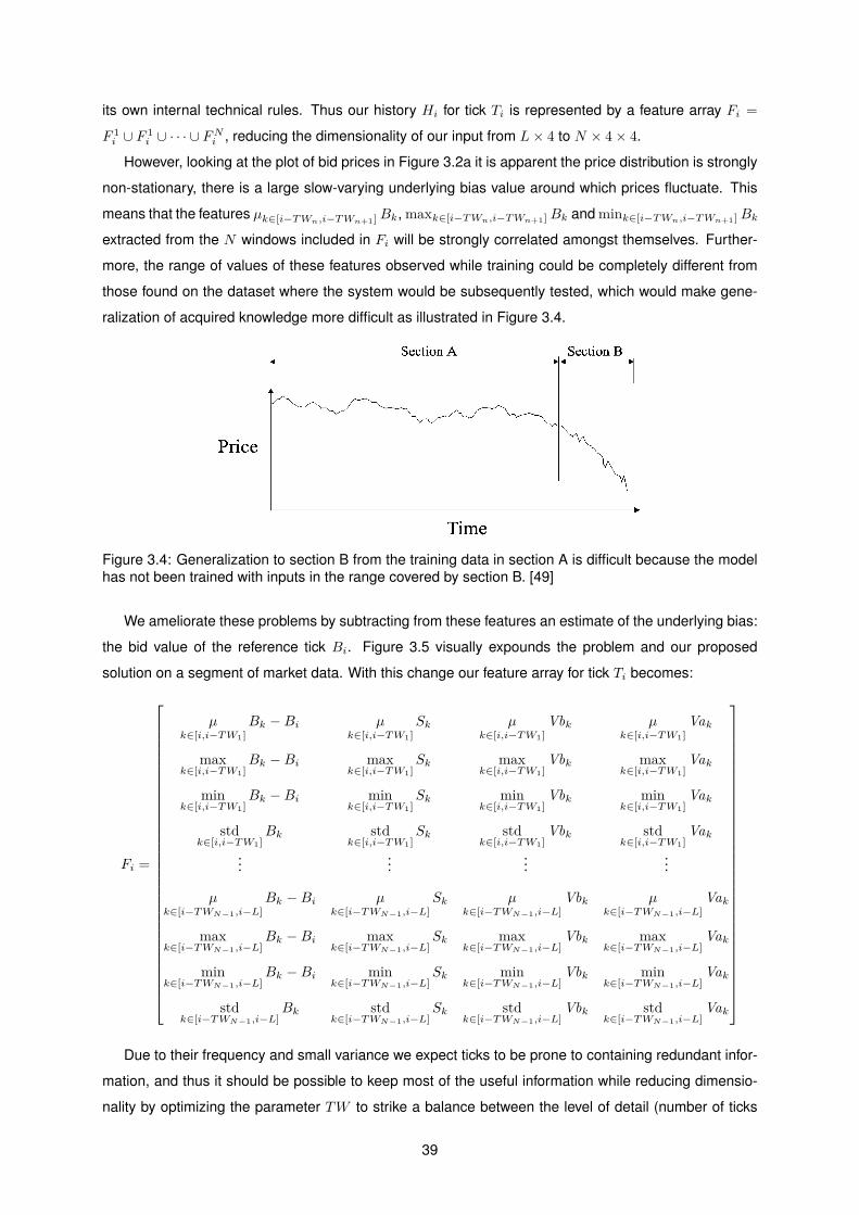
its own internal technical rules. Thus our history Hi for tick Ti is represented by a feature array Fi =

F 1i ∪ F 1

i ∪ · · · ∪ FNi , reducing the dimensionality of our input from L× 4 to N × 4× 4.

However, looking at the plot of bid prices in Figure 3.2a it is apparent the price distribution is strongly

non-stationary, there is a large slow-varying underlying bias value around which prices fluctuate. This

means that the features µk∈[i−TWn,i−TWn+1] Bk, maxk∈[i−TWn,i−TWn+1] Bk and mink∈[i−TWn,i−TWn+1] Bk

extracted from the N windows included in Fi will be strongly correlated amongst themselves. Further-

more, the range of values of these features observed while training could be completely different from

those found on the dataset where the system would be subsequently tested, which would make gene-

ralization of acquired knowledge more difficult as illustrated in Figure 3.4.

Figure 3.4: Generalization to section B from the training data in section A is difficult because the modelhas not been trained with inputs in the range covered by section B. [49]

We ameliorate these problems by subtracting from these features an estimate of the underlying bias:

the bid value of the reference tick Bi. Figure 3.5 visually expounds the problem and our proposed

solution on a segment of market data. With this change our feature array for tick Ti becomes:

Fi =

µk∈[i,i−TW1]

Bk −Bi µk∈[i,i−TW1]

Sk µk∈[i,i−TW1]

Vbk µk∈[i,i−TW1]

Vak

maxk∈[i,i−TW1]

Bk −Bi maxk∈[i,i−TW1]

Sk maxk∈[i,i−TW1]

Vbk maxk∈[i,i−TW1]

Vak

mink∈[i,i−TW1]

Bk −Bi mink∈[i,i−TW1]

Sk mink∈[i,i−TW1]

Vbk mink∈[i,i−TW1]

Vak

stdk∈[i,i−TW1]

Bk stdk∈[i,i−TW1]

Sk stdk∈[i,i−TW1]

Vbk stdk∈[i,i−TW1]

Vak...

......

...

µk∈[i−TWN−1,i−L]

Bk −Bi µk∈[i−TWN−1,i−L]

Sk µk∈[i−TWN−1,i−L]

Vbk µk∈[i−TWN−1,i−L]

Vak

maxk∈[i−TWN−1,i−L]

Bk −Bi maxk∈[i−TWN−1,i−L]

Sk maxk∈[i−TWN−1,i−L]

Vbk maxk∈[i−TWN−1,i−L]

Vak

mink∈[i−TWN−1,i−L]

Bk −Bi mink∈[i−TWN−1,i−L]

Sk mink∈[i−TWN−1,i−L]

Vbk mink∈[i−TWN−1,i−L]

Vak

stdk∈[i−TWN−1,i−L]

Bk stdk∈[i−TWN−1,i−L]

Sk stdk∈[i−TWN−1,i−L]

Vbk stdk∈[i−TWN−1,i−L]

Vak

Due to their frequency and small variance we expect ticks to be prone to containing redundant infor-

mation, and thus it should be possible to keep most of the useful information while reducing dimensio-

nality by optimizing the parameter TW to strike a balance between the level of detail (number of ticks

39

(a)

(b)

Figure 3.5: Features extracted from the same segment of data as Figure 3.3, divided into 500-tickwindows. (a) shows the original features and (b) depicts our solution to the non-stationarity.

40

per window), the scope (total number of ticks included) and the dimensionality (number of windows) of

our compact representation of history H.

A final addition to the feature array, is the time at which tick Ti was put out. The market behaves

slightly differently according to the hour of the day mainly due to the working hours of the major trading

capitals: Sydney, Tokyo, London and New York. This can result in consistently higher volume and vola-

tility at certain times, and thus we want to relay that information to the system to aid in its interpretation

of the market. We use the following two input variables to encode the hour:

time1i = sin(2π secondsi86400 ) (3.2)

time2i = cos(2π secondsi86400 ) (3.3)

where secondsi is the time when the reference tick was put out converted to seconds. This encoding

method effectively conveys the cyclical nature of hours to the neural network.

3.2.2 Standardization

We aim to standardize the variables in the feature array to meet the criteria introduced above. We do

this via a linear transformation known as min-max normalization:

midrange = maxi xk,i + mini xk,i2 ,

range = maxixk,i −min

ixk,i,

fk,i = xk,i −midrangerange/2 .

(3.4)

where xk,i is the kth element of Fi and sk,i is its normalized counterpart3.

While min-max does not ensure that the mean of each variable over the training dataset will be zero,

as a z-score normalization would, it keeps the range of input variables thoroughly predictable in the

range fk ∈ [−1, 1],∀i which is very helpful for stability and debugging of gradient descent learning. Also,

it keeps the distribution of each input variable intact making no assumptions or requiring any model for

market behavior. It is not robust to outliers however, any large outlier will skew the main body of the

distribution, which becomes confined to a small slice of the available range. This would lead to a loss of

sensitivity that could render the neural network unable to extract meaning from that input variable.

This is problematic since we expect large outliers in most foreign exchange datasets. Firstly because

retail level currency trading stops during the weekend but the interbank market continues to trade. Since

the first closely follows the second, when trading resumes prices and volumes may be significantly

changed as if there were two days of trading, although from a retail perspective the last tick before the

weekends and the first one after are contiguous. Features extracted from tick windows that include this

gap can become outliers, particularly for standard deviation features and for our bid price features due

3Note that the hour features are normalized by default.

41

to a possible subtraction with a price that effectively occurred two days after. Secondly, significant real

world events or movements by big players may trigger rare spikes of extreme volume accompanied by

sharp spread changes from the broker. Figure 3.6 shows the distribution of all the features introduced

in the previous section, excluding the time, extracted from 500-tick windows over roughly one year of

market data.

Figure 3.6: Distribution of the unstandardized feature variables extracted from 500 tick windows fromroughly one year of bid (red), bid volume (green), ask volume (cyan) and spread (blue) data. X-axis ofeach distribution is bounded to the maximum and minimum value, so all values depicted have at leastone occurrence even if not visible on the Y-axis due to scale. Raw data from the EUR/USD pair during2013 from Duskacopy broker.

As expected it is clear that in most cases there are a number, albeit minute, of occurrences far outside

the range occupied by the rest of the distribution. Since we simply want to curtail the impact of these

occurrences while maintaining the distribution mostly intact, we apply a simple percentile-based filter.

The qth percentile of feature xj , qth(xj), is computed as the value q100 of the way from the minimum to

the maximum of a sorted copy of an array containing all entries of the feature for a dataset. The filter

rule used is:

xj,i =

(1− q)th(xj), if xj,i < (1− q)th(xj)

qth(xj), if xj,i > qth(xj)

xj,i, otherwise

(3.5)

42

where q should be set conservatively to only target the most outlying values. The price for this filtering

is loss of sensitivity within these extreme values. Applying this filter, followed by the normalization

described in Equation 3.4 we obtain the final features, whose distributions for the same conditions as

above are shown in Figure 3.7.

Figure 3.7: Distribution of feature variables, extracted from the same raw data as Figure 3.6, filtered,with q = 99, and standardized. Bid (red), bid volume (green), ask volume (cyan) and spread (blue) data.

Upon inspection of Figure 3.7 and empirical testing, features mink∈[i−TWN−1,i−L]

Sk, mink∈[i−TWN−1,i−L]

Vbkand min

k∈[i−TWN−1,i−L]Vak were removed from the feature array as they appear to not contain useful

information and simply contributed to overfitting.

3.3 Market Simulation

With the market simulation we want to create an environment to coordinate the flow of information that

reaches the system so that it follows the reinforcement learning paradigm, which means supplying the

system with a state, receiving its response in the form of an action and answering with a new state and

a reward. Also, this process must be consistent with trading in the real foreign exchange market, so that

its learned behavior and our measure of its performance would translate to real trading.

The market simulation follows prices from a tick dataset T = {T0, .., TD}. The system is only al-

43

lowed to make a decision every time skip ticks. At each step/interaction4 t the market environment

is at the price in tick Ti=t·time skip+b, where b is the chosen starting tick for the first interaction, and

sends the system the state St. The parameter time skip and starting point b are further explained in

subsection 3.3.1.

A response is received in the form of an action signal At, after which the market environment skips

to the price in Ti+time skip and drafts a new state St+1 and a scalar reward Rt+1 for the action At,

which are sent to the system. State and reward signals are produced with the functions described in

subsection 3.3.2 and subsection 3.3.3 respectively.

These interactions continue until the end of dataset is reached, completing what is referred to as a

pass through the dataset. There are two types of passes, firstly training passes where the actions se-

lected by the system have an exploratory component and observed experiences et = (St, At, Rt+1, St+1)

are stored and used to update the network weights. Secondly, test passes where the system always

chooses what it believes to be the best action and no updates are performed to the Q-network. While

training passes always use a training dataset, test passes are performed on both a training dataset and

a validation dataset for assessing quality of learning, as described in subsection 3.3.4, and on a test

dataset to estimate real financial performance, as described in chapter 4.

3.3.1 time skip and nr paths

Most trading systems use hourly, daily, weekly or monthly data, which means they make decisions with

a hourly, daily, weekly or monthly time gap. As we are using tick data, without a time skip parameter

it would make a decision with the time gap of a tick. Since ticks can happen extremely fast this is

impractical. The latency of the connection between system and broker is much too high for realistic

execution of such orders. Also, a system allowed to trade at such velocity would have a larger effect on

the market, even in one as liquid as this one, and the assessment of performance would lose predictive

value.

Thus we only allow the system to make a decision at every time skip ticks. We chose time skip =

5000, which on average is somewhat less than two hours for 2013 EUR/USD tick data, since it fits

with our aim of a short term speculator without being so high frequency as to be too affected by practical

concerns such as latency and lack of broker liquidity. This value was chosen a priori, with no optimization

involved, and treated as a trader’s preference choice since the process to optimize the system for a

variety of trading frequencies would be too lengthy with our computational resources. Other users could

simply adjust time skip to suit their own trading frequency preference, although the rest of our system’s

parameters were optimized with time skip = 5000 in mind and would likely require readjustment.

Intuitively, an advantage of using ticks with a time skip parameter rather than directly use data with

the desired time gap, is that with this approach the periodicity of decision-making is not a fixed interval

as for most systems in the literature. When the market is more active, time skip represents a smaller

interval of time, while for periods of little activity time skip is a much larger time gap between decisions.

4Which only happen every time skip ticks.

44

This means that the system, for lack of a better term, pays more attention to the market when it should

be paying more attention.

A more significant advantage is the possibility of carving different paths through the data. By chan-

ging the starting point of a training or testing pass through the data to Tb with:

b ∈ {x · time skipnr paths

| x ∈ N0, x < nr paths }, (3.6)

we change the whole set of market states visited on that pass, as shown schematically in Figure 3.8.

T0 T1 T2 T3 T4 T5 T6 T7 T8 T9 T10 T11 T12 . . .

T0 T1 T2 T3 T4 T5 T6 T7 T8 T9 T10 T11 T12 . . .

Figure 3.8: Schematic of a dataset of ticks and how the market environment sequentially visits thoseticks through two different paths, in orange and black. Top: time skip = 2, Bottom: time skip = 4.These paths would be very similar, but for larger values of time skip the distance between ticks visitedin different paths increases and so does the quality of information added by having different paths.

By using a different path through the data each time we train the network, we supply the system with

a larger variety of data. Neural networks are known to require large amounts of data, especially as their

complexity increases, thus this approach helps mitigate overfitting and increases generalization capabi-

lity. Figure 3.95 exemplifies this effect: performance in the validation dataset improves and overfitting is

delayed and less severe.

This advantage also extends to testing the system. The standard testing approaches deliver a path-

dependent distribution of gains thus increasing the chances of a ”lucky” trading strategy. This is regarded

as a serious problem in testing trading systems [50], which we also mitigate through this various paths

approach. For each test we perform a number of test passes through different paths and use the

resulting average as the result of that test. It stands to reason that a system performing well through a

variety of initial conditions is a better predictor of future success. This also provides rigor to testing, as

the standard deviation of performance over the different paths gives us a measure of the uncertainty of

these tests.

nr paths linearly increases computational time and it has diminishing returns as paths become more

similar between them and thus increasingly redundant. We have found nr paths = time skip500 , meaning a

distance of 500 ticks between paths, is a balanced value for both testing and training passes, and use

it throughout this work. We define nr paths to keep a certain tick distance between paths rather than

as a fixed value, ie. nr paths = 2, to allow a user to seamlessly lower or increase trading frequency,5Note this figure was obtained as part of the optimization process and does not use the last iteration of the system.

45

(a) With nr paths = 1. (b) With nr paths = 10.

Figure 3.9: Example of learning curves with and without the nr paths dynamic. Training dataset:01/2011 to 01/2012. Validation dataset: 01/2012 to 07/2012. How these learning curves are produ-ced is further explained in subsection 3.3.4.

by changing time skip, while keeping the amount of ”unique” data the Q-network is trained on constant.

This opens the door to training the Q-network to trade at frequencies that would otherwise not offer

enough data points, within certain limits of course, the data thus generated has some redundancy, it is

not of the same quality as truly new data.

3.3.2 Reward Signal

The initial approach for the reward signal was to use only the profit obtained from each transaction. This

approach is intuitive, simple to implement and imposes no constraints to the system on how to achieve

profitability. However, tests revealed it introduced consistent behavioral flaws. Since the system was

not punished for holding positions with negative unrealized profits, but was punished at moment of their

closing, it learned to keep a position open until its unrealized profit bounced back to positive values

however long that may take, as observed in Figure 3.10.

Figure 3.10: Behaviour with the initial reward approach on a 6 month validation dataset from 2012.01to 2012.06. Each step skips 5000 ticks. Green arrows are long positions and red arrows are shortpositions.

Obviously, this is a critical flaw, the asset may never regain its former value or take so long to do

so as to make the system inviable. To solve this issue a new reward component was added: the

46

variation of unrealized profit, to which we refer as the return. Actions At that create a return, opening

a position and holding a position open, are rewarded with the magnitude of that return: the difference

between the unrealized profit in the state St in which they were taken and the unrealized profit in the

state St+1 to which they lead. Both approaches obtain similar profit, but various tests showed the second

approach effectively corrects for the behavior flaws previously observed as exemplified in Figure 3.11,

which means that profit is obtained with less risk. Furthermore, its seems that the increase in feedback

given to the system alleviates the credit assignment problem as various tests show the system’s learning

curve develops in a significantly smaller number of epochs.

Figure 3.11: Example of behaviour with the final approach to reward on a 6 month validation datasetfrom 2012.01 to 2012.06. Each step skips 5000 ticks. Green arrows are long positions and red arrowsare short positions.

We saw in section 2.4 that some systems use risk-adjusted profit as their reward. The most common

methods to adjust for risk are the Sharpe ratio, which divides the profit by the standard deviation of

unrealized profit, and its modification the Sortino ratio, which divides profits by the downside deviation

of unrealized profit. Both aim to penalize large variations of unrealized profit which are interpreted as

risk. Our reward system is in essence very similar, especially to the Sortino ratio since positive volatility

is not punished, as is the case with the Sharpe ratio, but rewarded. The difference is that rather than

introduce the punishment/reward at the end of the transaction by adjusting the profit, it is spread out

over its life with the return at each step, which has the empirically observed benefit of speeding up the

learning process, possibly by alleviating the credit assignment problem.

Algorithm 1 describes in pseudocode the implementation of a function that creates such a reward

signal. Notice that the reward derived from the profit or the return is, through min-max normalization,

always in the range [−1, 1] for each dataset T. This makes learning more stable by limiting the size of the

cost function gradients [6]. Also, it becomes easier to find suitable hyper-parameters for the system and

allows the use of those same hyper-parameters across a variety of datasets with different profit/return

distributions and with different position size.

Also, similarly to the standardization performed in subsection 3.2.2, we apply a percentile filter to

values above a certain percentile return percentile of absolute return before normalizing them with

the min-max method, since weekend-gaps in T create returns that significantly skew the distribution as

observed in Figure 3.12. This is not an issue for the profit reward, to which we simply apply a min-max

normalization directly. The use of the return percentileth also allows us to control how much importance

47

Algorithm 1 Compute reward Rt+1 for action At in state St

Precondition: max r is the return percentileth percentile of the absolute distribution of returns in thetraining dataset.

Precondition: max p is the maximum possible profit in the training dataset.1: function REWARD(unrealized profitt, unrealized profitt+1, At)2: if At = Open Long or At == Open Short or At == Hold Position then3: return← unrealized profitt+1 − unrealized profitt4: Rt+1 ← sign(return) ∗min(abs(return/max r), 1)5: else if At == Close Long or At == Close Short then6: Rt+1 ← sign(unrealized profitt) ∗min(abs(unrealized profitt/max p), 1)7: else8: Rt+1 ← 09: end if

10: return Rt+111: end function

the system gives to return rewards compared to profit rewards, as a tighter percentile filter equates to

larger return rewards.

(a) Without percentile filter. (b) With return percentile = 99.

Figure 3.12: Distribution of possible returns in a EUR/USD Duskacopy dataset of the year 2013, withtime skip = 500.

3.3.3 State Signal

In this section we describe the state signal created by the market environment. A pseudocode imple-

mentation is provided in algorithm 2.

The dataset T = T0, .., TD used by the market environment to set the prices has a counterpart

F = F0, .., FD created from it by the preprocessing procedure described in section 3.2. Its element

Fi=t·time skip+b, containing the compact representation of the market history associated with the current

tick Ti, is a component of the state St.

A second component of St is an integer scalar ht with three discrete values, whose purpose is telling

48

Algorithm 2 Assemble state StPrecondition: max p is the maximum possible profit in the training dataset.Precondition: Bidk and Askk are the Bid and Ask prices from the kth tick in the dataset.Precondition: Fk is the feature array for the kth tick in the current dataset.

1: function STATE(St, At,T,F)2: St+1 ← [0, 0, 0, 0]3: if At == Open Long then4: St+1[0]← 15: Askopen ← Askt·time skip+b6: else if At == Open Short then7: St+1[0]← −18: Bopen ← Bt·time skip+b9: else if At == Hold or At == Idle then

10: St+1[0]← St[0]11: else if At == Close Long or At == Close Short then12: St+1[0]← 013: acc size← acc size+ unrealized profitt14: end if15: if St+1[0] == 1 then16: unrealized profitt+1 ← position size · (Bid(t+1)·time skip+b −Askopen)17: else if St+1[0] == −1 then18: unrealized profitt+1 ← position size · (Bidopen −Ask(t+1)·time skip+b)19: else if St+1[0] == 0 then20: unrealized profitt+1 ← 021: end if22: St+1[1]← sign(unrealized profitt+1) ·min(abs(unrealized profitt+1/max p), 1)23: St+1[2]← min(max(−1, 2 · (((acc size+ unrealized profitt+1)/init acc size− failure)/(safe−

failure)− 1), 1)24: if St+1[2] == −1 then25: Flag St+1 as terminal.26: end if27: St+1[3]← F(t+1)·time skip+b28: return St+129: end function

the system if it currently has a position open and of which kind:

ht =

1, if long position open

0, if no position open

−1, if short position open

(3.7)

A third component is a float scalar vt containing the unrealized profit of the currently open position,

normalized in the same manner as the profit reward described in subsection 3.3.2. Thus vt is meant to

convey the system how much reward it will receive by closing the currently open position.

The fourth and final component of the state signal is a float scalar ct which tells the system the

current size of the account, including the unrealized profit of any open position, compared to the initial

size. This value is normalized and clipped to the range [−1, 1], where the maximum and minimum

49

represent, respectively, a safe level and a failure level, both set by the user:

ct =

1, if AccountSize

InitialAccountsize > safe

−1, if AccountSizeInitialAccountsize < failure

2 · ( AccountSizeInitialAccountsize − failure)/(safe− failure)− 1, otherwise.

(3.8)

The goal of this component is to introduce a condition for a terminal state. In RL the terminal state is the

last in a chain of interactions, and thus is state with a precisely known Q-value: the reward obtained in

that state, since no further rewards will be earned. It can thus act as an anchor for learning. Should the

current account size reach the failure threshold, the system flags it as a terminal state6. After a state

is flagged as terminal, the account size is reset to the initial value and training continues.

The terminal state condition was added for its value anchoring effect and to further punish strings of

consecutive bad decisions, common in the early stages of training. Empirically we verified that a failure

threshold closer to 1, meaning more instances of terminal states, does increase learning speed. But if it

is set too close to 1 it diminishes leaning quality. Thus, we set failure to 0.8, which modestly increases

learning speed while safely out of the range where learning quality starts to suffer. The safe threshold

is simply for normalization purposes, and was set to 2.

3.3.4 Training Procedure

The training procedure is structured into epochs. Each epoch has four distinct phases, a learning phase

and three phases to assess learning progress:

• Training pass over a training dataset (learning phase);

• Evaluation of Q-values over random set of states (first metric);

• Test over the training dataset (second metric);

• Test over the validation dataset (third metric).

The procedure, excluding the first metric, is depicted schematically in Figure 3.13. For the first metric,

states are collected by running a random policy through the training dataset and then at each epoch

we assess the Q-Network’s average estimated Q-value for that set of states. A smooth growth in this

metric, with no divergence, suggests that the Q-Network is learning and stable. This metric is useful for

debugging in early stages of system development where learning is still unstable and design choices

must be taken to improve its stability, but in later stages it is no longer necessary and was eventually put

aside to speed up training execution. Thus this metric does not feature throughout the rest of the thesis

and is mentioned here simply for completeness.

For the second and third metrics the profit generated over the test is recorded and the evolution of

that profit over the epochs is the indicator of how well the system is learning. In the case of the third

metric, we are testing on data, the validation dataset, that the system does not access while training.6See algorithm 3 for the implementation.

50

Epoch

TrainingPass

Testing passon

training dataset

Testing passon

validation dataset

Bestvalidation?

Save modelas

current candidate

Early stop?

Output current candidate as final model

yes

no

no

yes

Figure 3.13: Training Procedure.

The validation dataset corresponds to a period of time immediately following the training dataset. The

aim is to make sure that what our system is not only learning how to behave when confronted with the

training dataset, but that what it learns will generalize to data it has not seen during training. Relying

only on training dataset performance could be misleading as it is possible that the progress observed

for the training dataset comes from learning the idiosyncrasies of that dataset, its noise, rather than the

underlying relationships, an issue known as overfitting. This metric is the crux of the learning process,

since it is performance on previously unseen data that we truly want when subsequently applying the

system to live training. We rely on the validation performance curve to tell us when to stop training i.e.

how many epochs to train for, via the early stopping approach.

With early stopping, each time the performance assessment on the validation reaches a new high we

save the current model7 as our candidate to final model and a counter is started. This counter is reset

when a new candidate appears, but if that counter reaches predefined limit then the training process is

7By model we mean the Q-network with a given set of weights. After each epoch that set of weights has changed and so weconsider it a new model.

51

stopped early and the current saved candidate is our final model. This is an inexpensive way to avoid

strong overfitting even if the other hyper-parameters would yield to overfitting [32].

3.3.5 Example

In this section we aim to make clearer how the procedures introduced so far interact to create the

market environment for our Q-network. To do so, we provide a slightly scaled down example with TW =

[0, 4000, 6000], time skip = 5000, nr paths = 10, init acc size = position size = 10000, a training

dataset with 5,000,000 ticks and a validation dataset with 1,000,000 ticks.

According to the parameter TW , 6,000 ticks are necessary to create a feature vector thus our market

simulation has to start each pass, at the earliest, from tick Ti=6000. This is simply a practical detail and

was overlooked in the notation introduced in the sections above to avoid further cluttering. Firstly, the

training pass starting from step t = 0. The initial tick is Tb with b ∈ {x · 500 | x ∈ N0, x < 10 }, and

thus for this first pass training pass we start from T0, which is actually T6000 due to the aforementioned

practical consideration. Preprocessing creates the first feature array F6000:

µk∈[6000,2000]

Bk −B6000 µk∈[6000,2000]

Sk µk∈[6000,2000]

Vbk µk∈[6000,2000]

Vak

maxk∈[6000,2000]

Bk −B6000 maxk∈[6000,2000]

Sk maxk∈[6000,2000]

Vbk maxk∈[6000,2000]

Vak

stdk∈[6000,2000]

Bk stdk∈[6000,2000]

Sk stdk∈[6000,2000]

Vbk stdk∈[6000,2000]

Vak

mink∈[6000,2000]

Bk −B6000 µk∈[2000,0]

Bk −B6000 µk∈[2000,0]

Sk µk∈[2000,0]

Vbk

µk∈[2000,0]

Vak maxk∈[2000,0]

Bk −B6000 maxk∈[2000,0]

Sk maxk∈[2000,0]

Vbk

maxk∈[6000,2000]

Vak stdk∈[2000,0]

Bk stdk∈[2000,0]

Sk stdk∈[2000,0]

Vbk

stdk∈[2000,0]

Vak mink∈[2000,0]

Bk −B6000 time16000 time2

6000

which is fed to the state function from the market environment. The state function adds to the feature

array the components h0 = 0 and v0 = 0, since there is no position open, and c0 = 2 · (1 − 0.8)/(2 −

0.8)− 1 = −0.667, creating the state:

S0 =[0 0 −0.667 F6000

]

.

The Q-network is initialized with a random set of weights W0. It performs a forward propagation with

S0 and outputs its estimation for the action value of each possible action Q(St, an;W0), with n ∈ [0, 1, 2].

The ε-greedy algorithm selects one of the actions action based on these values. Since there is no

position open: a0 represents opening doing nothing, a1 opening a long position and a2 opening a short

position. For this example let us assume the action selection chose A0 = a1, thus opening a long

position.

This action is passed on to the market environment. It is now step t = 1, and per the time skip

52

parameter the market is now in tick T11000. The chosen action A0 is given to the reward function, so R1

can be drafted. The reward for opening a long position is the variation of unrealized profit, which was

0 before, normalized to the range [−1, 1] in regard to max r, the return percentileth percentile of the

training dataset’s possible returns. The order to open a position was given in tick T6000 when the ask

price was 1.32655, for example, and we are now in T11000 where the bid price is 1.32454. Assuming

max r = 0.012 in this dataset:

R1 = return

maxr= position size ·B11000 −A6000

position size ·max r= −0.00201

0, 012 = −0, 1675 (3.9)

A new state S1 is also drafted. Preprocessing creates the new feature array F11000:

µk∈[11000,7000]

Bk −B11000 µk∈[11000,7000]

Sk µk∈[11000,7000]

Vbk µk∈[11000,7000]

Vak

maxk∈[11000,7000]

Bk −B11000 maxk∈[11000,7000]

Sk maxk∈[11000,7000]

Vbk maxk∈[11000,7000]

Vak

stdk∈[11000,7000]

Bk stdk∈[11000,7000]

Sk stdk∈[11000,7000]

Vbk stdk∈[11000,7000]

Vak

mink∈[11000,7000]

Bk −B11000 µk∈[7000,5000]

Bk −B11000 µk∈[7000,5000]

Sk µk∈[7000,5000]

Vbk

µk∈[7000,5000]

Vak maxk∈[7000,5000]

Bk −B11000 maxk∈[7000,5000]

Sk maxk∈[7000,5000]

Vbk

maxk∈[7000,5000]

Vak stdk∈[7000,5000]

Bk stdk∈[7000,5000]

Sk stdk∈[7000,5000]

Vbk

stdk∈[7000,5000]

Vak mink∈[2000,0]

Bk −B11000 time111000 time2

11000

to which the state function adds h1 = 1 and, assuming maxp = 1000, v1 = −20.1

1000 = −0.02, since there is

a Long position open, and c1 = 2 · (0.998− 0.8)/(2− 0.8)− 1 = −0.670 so that:

S1 =[1 −0.02 −0.670 F11000

]

With S1 and R1 the Q-network has the first experience e0 = (S0, A0, R1, S1) with which to learn. S1 is

inputted to the network which performs a forward propagation and starts a new interaction. This cycle is

repeated until tick T499600, step t = 998, when it is no longer possible to skip 5000 ticks. This concludes

the first training pass.

After a training pass the market environment performs test passes on the training dataset. The

interaction cycle is exactly the same, except that ε is set to 0 so that the action with best Q-value is

always chosen, and observed experiences et are not used for Q-network updates. When it reaches the

end of the pass, tick T499600 or step t = 998, it restarts from a new path, meaning a new initial tick Tb

with b ∈ {x · 500 | x ∈ N0, x < 10 } is chosen. It performs this new pass starting from T6500, then another

starting from T7000, until a final pass starting from T10500, while recording the profit obtained from each

of those passes.

After the last test pass with the training dataset, it is time for test passes on the validation dataset.

The same cycle as above, a pass starting from T6000 and finishing at T996000, or t = 198. Then another

53

pass starting from T6500, T7000, etc. recording the profit from each. After all validation test passes, the

first epoch is complete.

A second epoch starts with a new training pass. The only difference between this training pass and

the one from the previous epoch, is that this one starts from, T6500, the second path. The training pass in

the third epoch will start from T7000, in the fourth it starts from T7500, etc. eventually goes back to starting

T6000, then T6500 again and so on. This allows for the Q-network to always learn from data it has not

seen in a number of epochs, making it more difficult to ”memorize” and thus overfit, while being tested

on all data to ensure more accurate assessment of performance. Epoch after epoch this repeats itself,

until the early stop procedure stops it.

3.4 Q-Network

So far, we have gone into detail about the environment surrounding the trading system, and how it

controls the flow of information into it. Now we take take a closer look at the system itself. Its core is a

fully connected backpropagational neural network, depicted schematically in Figure 3.14. This network

is tasked with computing a function Q(s;Wk), where Wk is the set of weights and biases of the network

at iteration k.

The input layer has a number of neurons defined by the elements in our representation of the state

s of the market, which per the hyper-parameter TW chosen in section 3.5 results in 148 input neurons.

This input layer is followed by three hidden layers with 20 ReLU neurons each.

The ReLu activation function was chosen due to its documented superiority for training multi-layer

neural networks [51] over other widely used activations, such as hyperbolic tangent and logistic sigmoid.

Future developments in the field of neural networks may bring change, but currently the number of

hidden neurons and layers has to be determined empirically (see [32] for practical recommendations).

We did so using the datasets described in Table 3.2, used for all hyper-parameter selection. This process

was performed in tandem with the choice of parameter TW to make sure there was a balance between

power of the network and number of input variables. We found this balance hard to achieve and very

precarious, with the Q-network easily slipping into overfitting. This is not surprising given the noisy

nature of financial data.

Tests were performed with L1 regularization, L2 regularization and dropout regularization to help

prevent overfitting, but they were not successful and these methods were not included in the final ar-

chitecture. We found significant performance gain from the three hidden layer topology versus a two

hidden layer or a single hidden layer with the same number of total neurons, although adding a fourth

layer made training difficult and resulted in decayed performance.

Finally, the output layer has three neurons with linear activations:

a4j = net4j =

n∑i=1

a3i · w4

ji + b4j , (3.10)

since they are meant to represent action values which may take any real value.

54

...

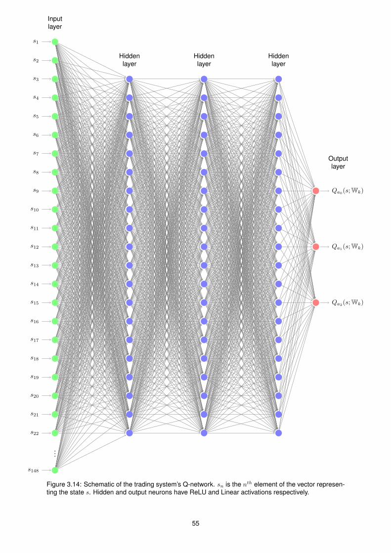
s1

s2

s3

s4

s5

s6

s7

s8

s9

s10

s11

s12

s13

s14

s15

s16

s17

s18

s19

s20

s21

s22

s148

Qa0(s;Wk)

Qa1(s;Wk)

Qa2(s;Wk)

Inputlayer

Hiddenlayer

Hiddenlayer

Hiddenlayer

Outputlayer

Figure 3.14: Schematic of the trading system’s Q-network. sn is the nth element of the vector represen-ting the state s. Hidden and output neurons have ReLU and Linear activations respectively.

55

With this topology have chosen to approximate the optimal action value function in its vectorial form:

Q(s;Wk) := (Qa0(s;Wk), Qa1(s;Wk), Qa2(s;Wk)) ≈ q∗(s) := (q∗(s, a0), q∗(s, a1), q∗(s, a2)), (3.11)

rather than the arguably more intuitive:

Q(s, an;Wk) ≈ q∗(s, an). (3.12)

The reasoning is that the second option would require a forward propagation to obtain the Q-value of

each action an, while this approach, first proposed by Mnih et al. [6], gives us all action values in a single

forward propagation, saving computational resources.

The above-described Q-network is initialized with a random set of weights where each weight is

drawn from an independent normal distribution with range [−1, 1]. Obviously this means its outputs are

initially completely random, and we need a process through which they can become better approxi-

mations of π∗. As per the interactions between system and environment described in section 3.3, the

Q-network collects experience at each step t in the form of transitions et:

et = (St, At, Rt+1, St+1). (3.13)

Looking back at standard tabular implementation of Q-learning (subsection 2.2.4), we would have a arbi-

trarily initialized table which after observing a transition et would use that experience to iteratively update

its tabulated estimate of q∗ for state St and action At, Qk(St, At), towards (Rt+1 + γmaxaQk(St+1, a)):

Qk(St, At)← (1− α)Qk(St, At) + α[Rt+1 + γmaxa

Qk(St+1, a)]. (3.14)

Our network aims to play the role of such a table, thus we apply the same concept in improving our neural

network’s approximation of q∗, but through the learning mechanisms of neural networks i.e. updating the

set of weights with backpropagation/gradient descent. et is given to a learning function which performs

these updates as described in subsection 3.4.1, an implementation specialized for stable Q-Network

learning.

3.4.1 Learning Function

The role of the learning function is to receive the transitions et observed during learning passes and

use them to change the Q-Network’s weights in a way that improves its approximation of q∗. A direct

adaptation of Equation 3.14 to the neural network learning methods introduced in the previous chapter

would suggest performing backpropagation/gradient descent updates, Equation 2.28 and Equation 2.32,

with a cost function such as:

Et(Wk) = ‖aLt,k − dt‖2 = (QAt(St,Wk)− (Rt+1 + γmax

aQa(St+1,Wk)))2. (3.15)

56

Note that dt is defined in such a way that outputs representing Q-values of the actions other than the

one responsible for transition et do not contribute to Et(Wk) and, by the extension, to the weight update.

This is generally the approach we take, but using a modified version of dt and an alteration to the typical

minibatch gradient descent implementation. Algorithm 3 describes our approach via pseudocode.

Algorithm 3 Use observed transitions to improve Q-Network

Precondition: e = [s, a, r, s′] is an observed transition.1: Initialize replay buffer with maximum capacity N2: Initialize updates = 0 and transitions = 03: function LEARN(et)4: transitions← transitions+ 15: if buffer is not full then6: Append et to buffer7: else8: Replace oldest element in the buffer with et9: end if

10: if transitions % update q == 0 then11: Sample random mini-batch Supdates of size B from buffer with elements ep = [sp, ap, rp, s′p]12: for each ep do13: if sp is terminal then14: set dp = rp

15: else16: set dp = rp + γQA(s′p,W−), with A = arg maxaQa(s′p,Wupdates)17: end if18: end for19: Compute

∑Bp=1

Ep(Wupdates)B

20: Perform backpropagation and RMSProp for Wupdates.21: updates← updates+ 122: end if23: if updates % update q− == 0 then24: W− ←Wupdates

25: end if26: end function

We introduce an auxiliary Q-Network, Q(s;W−), topologically identical to the original Q-Network,

whose weights W− are static and periodically copied from the original set Wk every update q− updates.

This auxiliary Q-network is used to generate the targets for updates:

Et(Wk) = (QAt(St,Wk)− (Rt+1 + γmaxa

Qa(St+1,W−)))2. (3.16)

The issue is that the original targets maxaQa(st+1,Wk) are constantly shifting in a correlated manner

with the Q-value estimations, which made learning more difficult and could easily spiral out of control

through feedback loops. This approach, first proposed by Mnih et al. [8], improves Q-Learning per-

formance and stability. We further improved upon Equation 3.16 through a variation known as double

Q-learning, suggested by van Hasselt et al. [11]:

Et(Wk) = (QAt(St,Wk)− (Rt+1 + γQa(St+1,W−)))2, with a = arg max

nQn(St+1,Wk). (3.17)

The aim of this change is to decouple, even if only partially, the action choice from the target Q-value

57

generation which is known to introduce a bias in the action value estimation resulting in poorer policies.

A final learning mechanism that has been found to by very helpful for Q-network learning, deals with

the composition of minibatch Sk used in the gradient descent algorithm (see Equation 2.32). Typically the

minibatch updates would happen in an online fashion, meaning that as training progresses the system

would sequentially collect |Sk| gradients, perform an update, discard them and then collect |Sk+1| more

and so on, synchronized with the stream of experience. However, this leads to two problems [52]:

• strongly correlated updates resulting in inefficient learning;

• the rapid forgetting of possibly rare experiences that would be useful later on.

For this reason we use a method known as experience replay [53] was introduced, whereby each expe-

rience et obtained is stored in a sliding window buffer of size N , from which a selection of B experiences

are randomly drawn every update q steps to perform a minibatch update. This ameliorates the issues

above and generally reduces the amount of experience required to learn.

3.5 Hyper-parameter Selection

Optimization of the system is based on the observed learning curves, particularly on the validation

datasets as they provide insight into the generalization power of the acquired knowledge. This means

that to assess each configuration of hyper-parameters we have to fully train the network. Depending

on the size of the dataset, the number of neurons in the Q-network and the parameters time skip and

nr paths it can take anywhere from a couple of hours to almost a whole day for a single test. Testing on

a single dataset is not enough since results are too dataset dependent and need to be confirmed. Also,

there is a large number hyper-parameters to tune and they are related to each other in complex ways:

by changing one of them, a number of the others may no longer be optimal. These factors have made it

impossible for us to perform a systematic grid search for the optimal set of hyper-parameters.

Instead, the values of hyper-parameters were selected by performing an informal search using the

three datasets described in Table 3.2, with the goal of obtaining the most stable learning curve with

the highest generalization capability, as measured by peak performance on the validation dataset. The

size and number of datasets was a compromise between testing on a meaningful amount of data and

completing the tests in a realistic time frame.

Dataset A Dataset B Dataset C

Training Validation Training Validation Training Validation

Begins 01/2011 01/2012 01/2012 01/2013 01/2013 01/2014

Ends 01/2012 06/2012 01/2013 06/2013 01/2014 06/2014

Nr. Ticks 25,786,841 11,507,313 23,467,196 8,723,458 18,643,628 5,884,697

Table 3.2: The three datasets used for hyper-parameter selection.

58

Hyperparameter Value Description

q 99 Percentile filter applied to extracted features.

time skip 5000 Number os ticks skipped between steps t and t+ 1.

nr paths time skip500 Number of different paths carved through the data

in training and testing passes.

return percentile 90 Percentile filter applied to the distribution of returnsin the dataset.

failure / safe 0.8 / 2.0 Parameters used in normalizing the account size forthe state signal and flagging terminal states.

update q 8 Number of observed transitions between gradientdescent updates.

update q− 5000 The frequency, in number of gradient descent upda-tes, with which the target network Q− is updated.

|S| = B 60 Number of elements in minibatch used for gradientdescent.

N 60000 Size of experience buffer from which minibatchesare randomly drawn.

γ 0.99 Discount factor used in the Q-learning algorithm.

α 0.001 Learning rate used in the RMSProp algorithm.

ε0 / εf 1 / 0.3 Initial and final value of the decaying ε in ε-greedy

init acc size 10000 Initial size of the trading account, in units of the basecurrency.

position size 10000 Number of units of base currency invested in eachtransaction.

Table 3.3: Hyper-parameters chosen for the trading system.

The hyper-parameters thus selected are detailed in Table 3.3, some of which merit some further

discussion. The purpose of having distinct account size and position size parameters in the system

is to allow for future implementation of a variable position size scheme to optimize profitability. Tests

performed in chapter 4 do not include such optimization, thus we set init acc size = position size so

that profits can be easily interpreted in relation to the initial available capital, which was was given the

placeholder value of 10,000. The RL discount rate parameter γ is close to 1, meaning future rewards

are weighed heavily. This reflects the fact that a successful transaction requires future-oriented decision

making. Parameter ε from ε-greedy action selection is made to decay over the training process so that

the system takes advantage of acquired knowledge proportionally to the quality of that knowledge.

As for the parameter TW , the array whose elements are the beginning and ending of each window

from which to extract features in number of ticks preceding the reference tick, the following values were

selected:

TW =[0 1 2 3 4 5 6 7 8 9 10 60

]· time skip2

, thus defined to allow a seamless transition to other time skip values. With that being said, in an ideal

59

situation, TW would be re-optimized for different trading frequencies.

Using this hyper-parameter configuration on the datasets described in Table 3.2 yielded the learning

curves shown in Figure 3.15. Three main observations can be made from these learning curves. Firstly,

Figure 3.15: Learning curves for dataset A (top), B (middle) and C (bottom) with position size = 10000.

learning is strongly dataset dependent, clearly some datasets generalize better to their validation than

others. In dataset A and B a peak validation profit of 795±2878 and 680±233 is reached before learning

is interrupted by the early stopping procedure. For dataset C on the other hand, a much higher validation

profit of 1458 ± 260 is reached, and by the end of the preset 200 epochs limit the system still appeared

8Error bars are not included in the validation curves to avoid excessive cluttering.

60

to be learning with generalization, with the early stopping mechanism not being triggered.

Secondly, there is a clear overfit to the training dataset. If we take into account that the validation

datasets are only 6 months long and thus extrapolate their results, we obtain yearly validation profitability

of 15.9±5.74%, 13.6±4.6% and 29.2±5.2% for datasets A, B and C respectively while training profitability

for those same datasets is 115.8± 6.4, 78.0± 3.9 and 179.7± 6.6. This was expected given the nature of

financial data.

The third and most important remark, is that training the Q-network does in fact translate into impro-

ved out-of-sample financial performance over the epochs, otherwise the validation curve would simply

be a random collection of points with no overarching positive direction. Knowing that our system is

able to learn and that what it learns is reflected in out-of-sample data allows us to proceed and test the

system on the previously vaulted data in an attempt to assess if it produces a positive expectation of

financial performance.

61

62

Chapter 4

Testing

In this chapter we test our system, implemented as described in the previous chapter, on the EUR/USD

currency pair. While performance on the validation dataset is a measure of generalization power, it

cannot be used to estimate performance during actual live trading. During the training procedure we are

observing the evolution of performance on the validation dataset, and purposefully choose the model

that offers best performance. This is obviously not possible for live trading, there is only the chance

to try one model. Thus, a test dataset is introduced to serve as an unbiased estimator of live trading

performance. After the training procedure takes place, the model with the best generalization power as

measured by the validation dataset is chosen and tested on the test dataset.

The premise is that a model that has learned to perform well on the training dataset and subse-

quently also performs well on a validation dataset, is more likely to then be profitable on the test dataset.

However, markets are known to be non-stationary [49] and if market dynamics change too much from

the training/validation period to the testing period, the model will not perform as expected.

While this risk is unavoidable, it can be ameliorated by having the training and validation dataset as

temporally close as possible to the test dataset so that market conditions have a smaller chance to have

significantly changed. To this effect, rather than simply dividing the whole span of the available data into

a single training, validation and test dataset, we perform the tests using a rolling window as described in

Figure 4.1.

Theoretically, the smaller we make each step forward of the rolling window, or in other words, the

smaller we make the size of the test dataset, the better we tackle the non-stationarity issue. However,

this does entail greater computational effort as a greater number of tests must be performed to cover

the same amount of time. Considering the running time of each test with our resources, we decided on

a test dataset size of 4 months.

The size of the training and validation datasets must also be considered. If they are smaller, the

data the network learns (training dataset) and the filter through which the model is selected (validation

dataset) should be more similar to the test dataset and thus suffer less from non-stationarity. On the

other hand, since market data is remarkably noisy, if the training dataset is too small it will simply learn

noise and lose generalization power, and if the validation dataset is too small, the overall performance

63

Figure 4.1: Rolling window approach to testing. Note that the training set includes both training datasetand validation dataset, while the test set is where the final model obtained with the training procedure isapplied to assess its ”true” performance. [49]

on the dataset is more easily influenced by noisy unpredictable events and will tend to select models that

randomly perform well on those events rather than those that truly generalize well. Moody [10] refers to

these opposing effects as the noise/non-stationarity trade-off. A training and validation dataset size of

24 and 6 months was chosen through informal testing with data from the year 2013.

In section 4.1 we describe the results of testing the system on post-2008 crisis EUR/USD pair data:

from 2010 to 2017. These tests are meant to assess the hypothetical validity of the trading system, to

confirm it has a positive expectation of gain, rather than trying to accurately project its revenue potential.

This means we are not trying to optimize execution: position sizing was set a priori and kept constant,

and no stop-loss or take-profit orders were used. Also, while bid-ask spread commission is included, the

volume commission is not, because the rates depend strongly on the specific trader’s resources.

4.1 5,000 time skip

4.1.1 Results

Below are the results obtained by our Q-network trading system for the EUR/USD currency pair in the

time period of 2010-2017 for time skip = 5000. In Table 4.1 each of the test datasets is described and

in Figure 4.2 a portion of the learning curves responsible for the selection of the final model for each of

the tests is displayed, with the rest included in appendix A.

A couple of exceptions to the standard size of 24 months of training and 6 months validation datasets

were made. For the three 2010 test datasets we curtailed the training and validation dataset size to avoid

including data from the 2008 crisis. For the 2011 p.3 test, the standard training/validation dataset size

resulted in the learning curves depicted in Figure 4.3. The validation performance only worsens with

training, making it difficult to select a candidate for testing. Simply halving the validation to a 3 month

period solved this issue, suggesting a portion of the removed 3 months was incompatible with the training

64

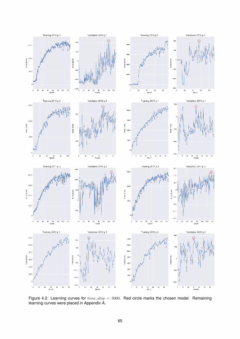
Figure 4.2: Learning curves for time skip = 5000. Red circle marks the chosen model. Remaininglearning curves were placed in Appendix A.

65

Test Name Begins Ends Nr. Ticks

2010 p.1 01/2010 05/2010 2,461,601

2010 p.2 12/2011 12/2011 2,475,378

2010 p.3 12/2012 12/2012 3,339,173

2011 p.1 01/2011 05/2011 6,564,138

2011 p.2 05/2011 09/2011 9,371,840

2011 p.3 09/2011 01/2012 9,866,644

2012 p.1 01/2012 05/2012 9,101,708

2012 p.2 05/2012 09/2012 8,497,184

2012 p.3 09/2012 01/2013 5,945,955

2013 p.1 01/2013 05/2013 7,013,688

Test Name Begins Ends Nr. Ticks

2013 p.2 05/2013 09/2013 6,454,267

2013 p.3 09/2013 01/2014 5,945,955

2014 p.1 01/2014 05/2014 4,549,733

2014 p.2 05/2014 09/2014 4,932,296

2014 p.3 09/2014 01/2015 7,538,760

2015 p.1 01/2015 05/2015 8,237,522

2015 p.2 05/2015 09/2015 8,419,406

2015 p.3 09/2015 01/2016 7,532,748

2016 p.1 01/2016 05/2016 9,779,630

2016 p.2 05/2016 09/2016 15,969,628

2016 p.3 09/2016 01/2017 19,281,366

Table 4.1: A description of the test datasets. Each one is referred to by year followed by quadrimester.

dataset. The final exception was the 2016 p.2 test. Inspection of Table 4.1 shows there was a marked

increase in tick density over the year 2016. We could not ascertain the reason for this increase, most

likely an internal change in the broker’s method of producing tick data. We halved the validation dataset

size for the 2016 p.2 test to include, proportionally, more data with the altered tick density so it would

select a candidate that performs well in these new conditions.

Figure 4.3: Learning curves for the 2011 p.3 test using the standard 24/6 months training/validation.

Choosing the candidate from each learning curve is straightforward for most cases, the one with best

validation performance. But in a few cases we have to take into account validation performance peaks

which arise from the fact that the neural network is randomly initialized and that learning with Q-networks

is a noisy procedure, as exemplified by Figure 4.4, taken from the original Atari playing Q-network paper.

This effect is exacerbated in the much noisier trading environment. Thus, to ensure the chosen model

is the product of actual learning rather than random oscillations or initialization, we ignore the first 10

epochs as candidates for final model. This is relevant for the 2014 p.3, 2015 p.3 and 2016 p.3 curves

and would have been in the case in 2011 p.1 and 2012 p.3 if the chosen peaks were slightly lower.

66

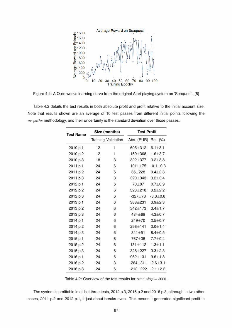
Figure 4.4: A Q-network’s learning curve from the original Atari playing system on ’Seaquest’. [8]

Table 4.2 details the test results in both absolute profit and profit relative to the initial account size.

Note that results shown are an average of 10 test passes from different initial points following the

nr paths methodology, and their uncertainty is the standard deviation over those passes.

Test NameSize (months) Test Profit

Training Validation Abs. (EUR) Rel. (%)

2010 p.1 12 1 605±312 6.1±3.1

2010 p.2 12 1 159±368 1.6±3.7

2010 p.3 18 3 322±377 3.2±3.8

2011 p.1 24 6 1011±75 10.1±0.8

2011 p.2 24 6 36±228 0.4±2.3

2011 p.3 24 3 320±343 3.2±3.4

2012 p.1 24 6 70±87 0.7±0.9

2012 p.2 24 6 323±218 3.2±2.2

2012 p.3 24 6 -327±78 -3.3±0.8

2013 p.1 24 6 388±231 3.9±2.3

2013 p.2 24 6 342±173 3.4±1.7

2013 p.3 24 6 434±69 4.3±0.7

2014 p.1 24 6 249±70 2.5±0.7

2014 p.2 24 6 296±141 3.0±1.4

2014 p.3 24 6 841±51 8.4±0.5

2015 p.1 24 6 767±36 7.7±0.4

2015 p.2 24 6 131±112 1.3±1.1

2015 p.3 24 6 328±227 3.3±2.3

2016 p.1 24 6 962±131 9.6±1.3

2016 p.2 24 3 -264±311 -2.6±3.1

2016 p.3 24 6 -212±222 -2.1±2.2

Table 4.2: Overview of the test results for time skip = 5000.

The system is profitable in all but three tests, 2012 p.3, 2016 p.2 and 2016 p.3, although in two other

cases, 2011 p.2 and 2012 p.1, it just about breaks even. This means it generated significant profit in

67

roughly 75% of the tests, and significant losses in only 14%, a good indicator of its validity.

The simple and compounded total test results are concisely described in Table 4.3. By simple, we

mean that profits are not reinvested, after each test whatever profits there may be are put aside and the

following test starts from the same initial conditions. From a financial perspective, investments are more

Compounding Total Absolute TestProfit (EUR)

Total Relative TestProfit (%)

Yearly Avg. TestProfit (%)

None 6782±977 67.8±9.8 9.7±1.4

Yearly 8982±1690 89.8±16.9 12.8±2.4

Triannual 9247±1802 92.5±18.4 13.2±2.6

Table 4.3: Simple and compounded total test profit for time skip = 5000.

often judged based on their compounded profit. Some trading systems use continuous compounding,

by including profits from a given trade in the position size of the next trade. We chose to use a fixed

position size during each test and compound between tests, ie. change the fixed position size at the

onset of a test by including the total profit of the previous tests in the account. Compounding increases

the overall profit, but also increases uncertainty ie. the risk of the trading system.

In Table 4.4 we look at the trades individually for a better insight into the behaviour of the system.

It is apparent that the system generally relies on a large number of small trades, roughly 550 trades

per year with 0.2% profit/loss per trade, which are profitable 53.5% of the time. There is a very slight

Trades

Total Profitable Unprofitable

Nr. 39287 21038 18249

Avg. profit (%) 0.017±0.384 0.215±0.337 -0.211±29.9

Avg. Duration 34788±87867 33679±96107 36066±77264

% Longs 49.2 48.8 49.6

Table 4.4: Trade-by-trade analysis for time skip = 5000. Note that trades from all 10 paths are included.Duration is in number of ticks.

tendency to favor the Short position in general, especially in trades that end up being profitable. This

can be explained by looking at the plot of EUR/USD prices in Figure 4.6, the Euro has on average been

losing value relative to the Dollar. The duration that each position stays open is similar in both profitable

and unprofitable trades, showing that the system has no problem cutting its losses and does not overly

wait for rebounds.

Figure 4.5 provides a sample of the system’s behavior in three different tests. For the most part the

system behaves as described, small trades in large numbers. However, that appears to change when

it detects a trend, switching to larger trade durations in a attempt to follow that trend, as observed 2011

68

Figure 4.5: System behaviour from 2011 p.1 (top), 2015p.3 (middle) and 2016 p.3 (bottom). Green andred arrows represent Long and Short positions respectively. Each step is 5,000 ticks apart.

69

p.1. In 2016 p.3 we can see how it displays an unusually large number of trades, leading to a gradual

accumulation of losses.

4.1.2 Result Analysis

In this section we take a closer look at the results presented above. We start by looking at the relationship

between validation and test performances. To that effect Table 4.5 contains the annualized results for

each validation/testing dataset pair. Annualized profit is an extrapolation of the profit obtained in a

dataset to what they would be over a year, assuming the same rate of gains, meant to allow comparisons

between datasets of different sizes.

Test NameValidation Profit Test Profit

Abs. (EUR) Annualized Abs. (EUR) Annualized

2010 p.1 441±173 52.9±20.8% 605±312 18.2±9.4%

2010 p.2 200±117 24.0±14.0% 159±368 4.8±11.0%

2010 p.3 806±320 32.2±12.8% 322±377 9.7±11.3%

2011 p.1 409±408 8.2±8.2% 1011±75 30.3±2.3%

2011 p.2 1387±211 27.7±4.2% 36±228 1.1±6.8%

2011 p.3 495±320 19.8±12.8% 320±343 9.6±10.3%

2012 p.1 1166±169 23.3±3.4% 70±87 2.1±2.6%

2012 p.2 897±184 17.9±3.7% 323±218 9.7±6.5%

2012 p.3 655±213 13.1±4.2% -327±78 -9.8±2.3%

2013 p.1 655±234 15.6±4.7% 388±231 11.6±6.9%

2013 p.2 520±151 10.4±3.0% 342±173 10.3±5.8%

2013 p.3 643±231 12.8±4.6% 434±69 13.0±2.1%

2014 p.1 196±38 3.9±0.8% 249±70 7.5±2.1%

2014 p.2 748±145 15.0±2.9% 296±141 8.9±4.2%

2014 p.3 461±89 9.2±1.8% 841±51 25.2±1.5%

2015 p.1 1189±51 23.8±0.1% 767±36 23.0±1.1%

2015 p.2 1267±76 25.3±1.5% 131±112 3.9±3.4%

2015 p.3 -57±306 -1.1±6.1% 328±227 9.8±6.8%

2016 p.1 745±210 14.9±4.2% 962±131 28.9±3.9%

2016 p.2 921±140 27.6±4.2% -264±311 -7.9±9.3%

2016 p.3 275±421 5.5±8.4% -212±222 -6.4±6.7%

Table 4.5: Comparison between validation and test results for time skip = 5000.

As expected, validation performance is for the most part superior to subsequent test performance.

Furthermore, simple observation of Table 4.5 seems to suggest that validation profit is not a good pre-

dictor of test profit. This is confirmed by a Pearson correlation coefficient of -0.28 at p-value significance

of 0.2, indicating no correlation between annualized validation and test profits. It is clear that the training

process creates a positive expectation for profits in a test setting, but results are too dataset dependent

to create an expectation on the magnitude of those profits.

70

On the other hand, the standard deviation between different paths obtained by the model in the

validation dataset compared to that of the test dataset has a Pearson correlation coefficient of 0.73 with

p-value significance 0.0002. This means that we can actually select stabler candidates based on the

validation process. Considering our total profit, with triannual compounding, has an uncertainty of almost

20%, our choice of candidate solely through peak validation performance was misguided, and exploring

this correlation could be an important avenue for improving the system’s performance.

We continue our result analysis by looking at equity growth trajectory. By equity we mean the current

size of the account plus the value of any currently open positions, relative to the initial account size. As

important as the final profit is, it is equally important the manner in which that profit level is reached.

If equity grows smoothly the risk the trading system presents is lower and the use of leverage can be

considered. On the other hand, if the equity growth curve contains large, frequent drawdowns, our

confidence in the trading system diminishes and the use of leverage must be kept to a minimum or none

at all. Drawdown is the difference between the equity size at a certain point and the size at the last equity

peak. It is one of the main measures of risk in financial trading. A drawdown of just 20% would empty a

trader’s account if he were to be using L = 5 leverage. Figure 4.6 shows the equity curve obtained by

our system, with the bid price over the 7 years of testing for context.

The equity curve is somewhat regular, with no extreme drawdowns at any point. This is made more

clear with Figure 4.7, which displays all drawdowns graphically, and Table 4.6 which discretizes the

maximum drawdown for each year along with that year’s test profit. The maximum drawdown was -

9.9±12.1, without compounding, and -16.6±20.0% with triannual compounding. These are relatively low

values, albeit with a large uncertainty due to how uncertainty is propagated, accumulating the uncertainty

from both the peak and the drought. This amount of drawdown would allow for a comfortable use of

leverage L = 2, which would have doubled our final profit.

YearTest Profit Maximum Drawdown

Abs. (EUR) Rel. (%) Abs. (EUR) Rel. (%)

2010 1086±612 10.9±6.1% -365±7270 -3.7±7.3

2011 1367±419 13.7±4.2% -825±1060 -8.2±10.6

2012 66±247 0.7±2.5% -900±1104 -9.0±11.0

2013 1164±297 11.6±3.0% -332±1115 -9.9±11.2

2014 1386±165 13.9±1.7% -258±1206 -2.6±12.1

2015 1226±256 12.3±2.6% -987±1213 -9.9±12.1

2016 487±404 4.9±4.0% -790±1359 -7.9±13.6

Table 4.6: Simple yearly profit and maximum drawdown for time skip = 5000.

It is hard to pin point the exact reasons why the year of 2012 stands apart from the the others in

terms of performance since a Q-network is a black box system. However, a closer look at Figure 4.6

can provide some speculation. Note that in 2012 there is for the most part no overall trend to the price

71

Figure 4.6: Bid prices for EUR/USD pair (top) and equity growth curve with and without compounding(bottom) for time skip = 5000. Light area around equity curves represents their uncertainty. X-axis is inunits of ticks.

Figure 4.7: Average drawdowns for time skip = 5000, uncertainty was not included for clarity. X-axis isin units of ticks.

72

changes, it mostly fluctuates inside a range and finishes the year close to the same value where it starts.

There is an exception in the middle of the year with a downwards trend followed by an upwards trend

where the equity grows, but it accumulates losses again with the sideways movement at the end of the

year. We can observe that this is mirrored in the year 2011 and 2015. While they are overall successful

years, those profits come from the beginning and the end of the year where there are clear trends.

In the middle part of both those years, where there is mostly sideways movement, there is little to no

equity growth. Possibly, when the market has a clear downward or upward trend there are distinguishing

patterns in the input features that allow exploitation, while more indecisive sideways periods result in

noisier inputs and poorer decisions.

The problem with the two final datasets, 2016 p.2 and 2016 p.3, is slightly different. While there is

also the problem of a mostly sideways moving market, it is exacerbated by the change in tick density by

the broker. Due to how our system is designed, larger tick frequency leads to larger trading frequency,

as Figure 4.5 showed. Thus, we have a system forced to trade much more frequently than intended in a

market context where it has been shown to struggle, which unsurprisingly results in losses.

This could be easily corrected by increasing the time skip parameter to 10,000 once the larger tick

frequency was detected. Rather than repeating only these two tests with time skip = 10000 we decided

to experiment with the rest as well. The reason for these tests is two-fold, firstly it serves as another

test to the system’s capabilities, should it obtain positive performance working under conditions it was

not optimized for, system’s validity is further supported. Secondly, in 2010 the tick density is roughly half

the rest of the datasets and the system performed well, which may indicate lowering trading frequency

could be beneficial.

4.2 10,000 time skip

For these tests with time skip = 10000, training and validation datasets as well as all other hyper-

parameters were unchanged from the previous approach. The exception is the nr paths parameter

which was defined in the previous chapter to keep the distance between paths at 500 ticks, and thus

also doubles to nr paths = 10000500 = 20.

4.2.1 Results

Figure 4.8 shows a portion of the learning curves responsible for the selection of the final model for

each of the tests, with the rest included in the appendix A. These learning curves were obtained using

the same training and validation datasets from the time skip = 5000 tests. The only difference is that

the year of 2010 is not included. Those tests used a much smaller training dataset to avoid 2008 data.

Furthermore this older data has less tick density. It was thus observed that, even with the nr paths dyn-

amic, there was difficulties in training the network at the time skip = 10000 frequency due to insufficient

datapoints.

In choosing the candidate from these learning curves the same consideration explained subsection 4.1.1

73

Figure 4.8: Learning curves for time skip = 10000. Red circle marks the chosen model. Remaininglearning curves were placed in Appendix A, as appendix.

74

Test NameSize (months) Test Profit

Training Validation Abs. (EUR) Rel. (%)

2011 p.1 24 6 1021±83 10.2±0.8

2011 p.2 24 6 -123±137 -1.2±1.4

2011 p.3 24 3 -26±364 -0.3±3.6

2012 p.1 24 6 58±299 0.6±3.0

2012 p.2 24 6 450±318 4.5±3.2

2012 p.3 24 6 -341±105 -3.4±1.1

2013 p.1 24 6 225±89 2.3±8.9

2013 p.2 24 6 485±181 4.9±1.8

2013 p.3 24 6 399±7 4.0±0.1

2014 p.1 24 6 173±47 1.7±0.5

2014 p.2 24 6 -392±61 -3.9±0.6

2014 p.3 24 6 722±76 7.2±0.8

2015 p.1 24 6 412±199 4.1±2.0

2015 p.2 24 6 143±258 1.4±2.6

2015 p.3 24 6 268±255 2.7±2.6

2016 p.1 24 6 445±276 4.5±2.8

2016 p.2 24 3 251±220 2.5±2.2

2016 p.3 24 6 337±198 3.4±2.0

Table 4.7: Overview of the testing procedure results for time skip = 10000.

applied in the case of 2016 p.3. Note that the disregarded validation performance peak in this case is

slightly out of the 10-epoch range we defined. Since each epoch contains a single learning pass, and

each pass with time skip = 10000 is smaller than time skip = 5000, it is actually within the range in

the measure that truly counts: amount of updates to the network. This is probably the same reason

why most learning curves with time skip = 10000 appear better behaved than their time skip = 5000

counterparts, each epoch or point in the graph represents a smaller number of updates smoothing the

behavior changes between epochs.

Table 4.7 details the performance obtained in both absolute profit and profit relative to the initial

account size. Considering that 2011 p.3 and 2012 p.1 just about break even, the system generated

significant profit in roughly 72% of the tests and significant losses in 16%. Once again, these numbers

suggest the validity of our trading system.

The simple and compounded total test results are concisely described in Table 4.3. Overall the results

are frankly inferior to the previous trading frequency, which is not particularly unexpected considering

the whole system was optimized with time skip = 5000 in mind. But they are nevertheless positive,

9.1±1.9% per year is still superior to most available financial applications.

With Table 4.4 we look at the trades individually while Figure 4.9 provides a sample of the system’s

behavior in three different tests. The system behaves very similarly to the time skip = 5000 case, with

two key differences. As expected the duration of each trade is roughly double that of the time skip =

75

Figure 4.9: System behaviour from 2011 p.1 (top), 2015p.3 (middle) and 2016 p.3 (bottom). Green andred arrows represent Long and Short positions respectively. Each step is 10,000 ticks apart.

76

Compounding Total Absolute TestProfit (EUR)

Total Relative TestProfit (%)

Yearly Avg. TestProfit (%)

None 4507±864 45.1±8.6 7.5±1.4

Yearly 5400±1244 54.0±12.4 9.0±2.1

Triannual 5457±1140 54.6±11.4 9.1±1.9

Table 4.8: Simple and compounded total test profit for time skip = 10000.

5000 system, which results in a larger average profit/loss per trade. And the total number of trades is

also roughly halved. With 2016 p.3 its seems that solving its excessive number of trades allowed the

system to become profitable once the market stopped moving sideways. The tendency to favor the Short

position is also more pronounced with this trading frequency. As we mentioned before, the overall trend

of EUR/USD has been for the Euro to lose value, and the overall trend becomes more important at lower

trading frequencies, which explains this growing asymmetry.

Trades

Total Profitable Unprofitable

Nr. 34445 17923 16522

Avg. profit (%) 0.026±0.517 0.299±0.471 -0.270±0.385

Avg. Duration 74364±220261 79445±263958 68852±159697

% Longs 47.2 47.4 46.9

Table 4.9: Trade-by-trade analysis for time skip = 10000. Note that trades from all 20 paths are included.Duration is the number of ticks during which a position was kept open.

4.2.2 Result Analysis

Table 4.5 contains the annualized results for each validation/testing dataset pair. The relationship bet-

ween validation and test performances observed with time skip = 5000 still holds for this new trading

frequency. There is a Pearson correlation coefficient of -0.31 at p-value significance of 0.21, once again

indicating that validation performance is not a good predictor of test performance. A correlation coef-

ficient of 0.67 at p-value significance of 0.002 for the uncertainties confirms the possibility of selecting

stabler candidates based on the validation process.

There is a significant correlation between validation performance from both trading frequencies, Pear-

son coefficient of 0.65 with 0.004 significance, and testing performance from both trading frequencies,

with a coefficient of 0.66 at 0.003 significance. This once again suggests that some datasets, ie. some

time periods of market behaviour, are inherently more predictable from technical data than others, which

is why test performance cannot be predicted by validation performance.

We continue our result analysis by looking at equity growth trajectory. Figure 4.6 shows the equity

77

Test NameValidation Profit Test Profit

Abs. (EUR) Annualized Abs. (EUR) Annualized

2011 p.1 613±233 12.3±4.7 1021±83 30.6±2.5

2011 p.2 1225±264 24.5±5.3 -123±137 -3.7±4.1

2011 p.3 893±279 35.7±11.2 -26±364 -0.8±10.9

2012 p.1 1191±294 23.8±5.9 58±299 1.7±9.0

2012 p.2 807±196 16.1±3.9 450±318 13.5±9.5

2012 p.3 695±235 13.9±4.7 -341±105 -10.2±3.2

2013 p.1 488±247 9.8±4.9 225±89 6.8±2.7

2013 p.2 150±213 3.0±4.3 485±181 14.6±5.4

2013 p.3 442±116 8.8±2.3 399±7 12.0±0.2

2014 p.1 778±82 15.6±1.6 173±47 5.2±1.4

2014 p.2 474±110 9.5±2.2 -392±61 -11.8±1.8

2014 p.3 438±107 8.8±2.1 722±76 21.7±2.3

2015 p.1 1139±129 22.8±2.6 412±199 12.4±6.0

2015 p.2 1232±175 24.6±3.5 143±258 4.3±7.7

2015 p.3 820±434 16.4±8.7 268±255 8.0±7.7

2016 p.1 822±312 16.2±6.2 445±276 13.3±8.3

2016 p.2 900±145 27.0±4.4 251±220 7.5±6.6

2016 p.3 397±315 7.9±6.3 337±198 10.1±5.9

Table 4.10: Comparison between validation and test results.

curve obtained by our system, with the bid price over the 6 years of testing for reference. The equity

curve confirms our previous observations that the system has its worst periods when the market is

moving sideways. This is clear in the middle of 2011, in 2012 with the exception of some growth when

there are clear trends in the middle, in the middle of 2015 and in the middle of 2016. The big difference

is that during the middle of 2016 it is no longer forced to trade at double the desired frequency, thus it

manages to break even rather than accumulate losses, and then make some gains at the end of the

year when a trend emerges.

Figure 4.7 displays all drawdowns graphically. Overall the drawdowns are very similar in magnitude

to the higher frequency system. The maximum drawdown was -10.9±4.2%, without compounding and

-11.9±4.5% with triannual compunding. The uncertainty is much smaller since the largest drawdown

occurs near the beginning of the equity growth curve, before the possible paths have diverged too much.

Again, these are low values which would probably allow for the use of a small amount of leverage.

To conclude this analysis, we look to the main motivation of testing the system with time skip =

10000, the two final datasets where tick density doubles. In Figure 4.12 we depict the equity growth

78

Figure 4.10: Bid prices for EUR/USD pair (top) and equity growth curve with and without compounding(bottom) for time skip = 10000. Light area around equity curves represents their uncertainty. X-axis isin units of ticks.

Figure 4.11: Average drawdowns for time skip = 10000, uncertainty was not included for clarity. X-axisis in units of ticks.

79

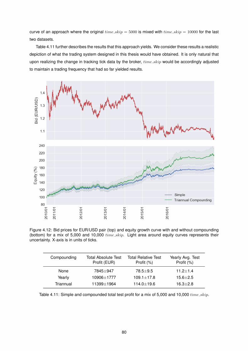
curve of an approach where the original time skip = 5000 is mixed with time skip = 10000 for the last

two datasets.

Table 4.11 further describes the results that this approach yields. We consider these results a realistic

depiction of what the trading system designed in this thesis would have obtained. It is only natural that

upon realizing the change in tracking tick data by the broker, time skip would be accordingly adjusted

to maintain a trading frequency that had so far yielded results.

Figure 4.12: Bid prices for EUR/USD pair (top) and equity growth curve with and without compounding(bottom) for a mix of 5,000 and 10,000 time skip. Light area around equity curves represents theiruncertainty. X-axis is in units of ticks.

Compounding Total Absolute TestProfit (EUR)

Total Relative TestProfit (%)

Yearly Avg. TestProfit (%)

None 7845±947 78.5±9.5 11.2±1.4

Yearly 10906±1777 109.1±17.8 15.6±2.5

Triannual 11399±1964 114.0±19.6 16.3±2.8

Table 4.11: Simple and compounded total test profit for a mix of 5,000 and 10,000 time skip.

80

Chapter 5

Conclusions

The main goals of this thesis were achieved. Learning in the training dataset is stable and it is apparent

from a number of validation learning curves that the Q-network is indeed capable of finding relations-

hips in financial data that translate to out-of-sample decision making. This speaks to the potential of

the neural network / reinforcement learning combo: this noisy, non-stationary environment is a far cry

from the deterministic Atari or Go environments, and still it was capable of learning performing policies.

Furthermore, this learning capability was successfully leveraged to produce positive financial gain in a

test setting.

It is difficult to compare our results with those obtained by other RL systems, being that there so few

examples of RL traders applied to the foreign exchange. In Table 3.2, the only RL system that uses a

modern dataset obtained a 1.64% profit for the year of 2014. For that same year we obtained 13,86%

without compounding. As for the remaining three systems, all RRL traders, our profitability is somewhat

in line with their results. Our results were obtained in a more challenging context however. Firstly our

tests cover a much much larger timeframe, which requires a more robust system that performs well

under a variety of market conditions. Secondly, as we saw in subsection 2.1.1, various sources indicate

that profitability derived from technical analysis methods has been declining sharply. These RRL traders

were tested with datasets ranging from 1996 to 2002, while our system was tested on contemporary

datasets.

However, it is not an approach that works well ”out-of-the-box”, we found it is not very robust at all.

Without a preprocessing stage and state function that ensured all inputs were within a contained range,

learning did not happen. Before ensuring outliers did not distort input variable distribution, learning was

unstable and out-of-sample performance was inconsistent, almost random. Reward normalization was

also essential, many attempts resulted in unstable or non-existent learning. Although RMSProp gives

it some robustness in terms of the learning rate parameter, other parameters concerning the network

updates such as the batch size, frequency of the updates of the target network or size of the buffer all

can easily derail learning if not appropriately set. Overall, it is a finicky, labour-intensive architecture.

Another drawback of this architecture, is that despite its success, it is difficult to extract insights as

it is very much a black-box approach. The final product is a trained network that provides no equations

81

or coefficients defining a relationship, beyond it’s own internal mathematics. The network is the final

equation of the relationship. It should be seen as an engineer’s tool, something with which to obtain

results since although there are efforts to ’gray the black-box’ [54], for the most part neural networks

with more than a couple of layers are as of now too complex to extract accurate insights. But the

architecture’s complexity may actually have played in its favour for this task. In subsection 2.1.1 we have

seen that there is somewhat of a consensus that potential profitability from technical analysis methods

has decreased over time, but more complex technical rules were more resistant to this efficiency of

the market. A network with three hidden layers such as ours has the potential to create fairly complex

internal technical rules, which may account for its continued profitability.

Overall, it is my opinion that this approach has a great deal of potential to be explored. There are

a number of probably sub-optimal parameters, chief among them the TW parameter controlling feature

extraction and the topology of the hidden layers. Furthermore there are design options, such as choice

of cost function or activation function of the hidden layers, that were not fully explored due to lack of

computational power to test configurations. These relatively small changes would certainly provide a

performance boost without even changing the overall architecture laid out in this thesis. In section 5.1

more in depth changes are discussed.

5.1 Future Work

Besides the already discussed incomplete optimization, there are two main weaknesses in this trading

system that should merit further work. Both concern how the displayed capacity to improve out-of-

sample performance by training can be turned into a profitable trading system in a test setting:

• Traning/validation/testing dataset choice: a more interesting alternative based on identifying mar-

ket regimes, for example, could be conjectured. Otherwise, our fixed size approach could be

improved by exhaustive search rather than our limited informal testing.

• Model candidate selection: our approach to choose the model with highest validation performance

was already shown to be overly simplistic in subsection 4.1.2, where it became clear that the

uncertainty the model presents in the validation dataset should have been taken into account.

The inclusion of this extra factor in the selection process would be a start, but more complex

selection methods could be tested. For example, rather than using just one candidate the trading

account could be split among a number of candidates which would help dilute the risk through

diversification.

Other than changes to the system itself, some possible future work could focus on improving the financial

facets of this work:

• Other types of financial data: the use of data classified as fundamental analysis, or simply market

data from other assets that correlate to the target asset, could improve performance. This would

not be a straightforward change however. Each extra input variable makes it easier for the system

82

to overfit the training data. We struggled in this thesis to achieve a balance between the neural

network’s power and the number of input variables to prevent, in so far as possible, overfitting. Any

additions to the input would have to contribute enough to overcome the extra overfit potential, and

would probably entail finding a new balance with neural network topology.

• Diversification: this is the most straightforward avenue for further work. There is no reason, in

theory, for this system not to work with other assets now that it has been shown to work with

EUR/USD, although it would almost certainly entail parameter re-optimization. These could be

other currencies or other financial objects altogether, from stocks to commodities, as long as there

is a large quantity of historical data for training.

• Execution: a layer for optimized execution could be added to control risk and maximize profitability

using, for example, variable position sizing and stop-loss/take-profit orders.

83

84

Bibliography

[1] A. P. Chaboud, B. Chiquoine, E. Hjalmarsson, and C. Vega. Rise of the machines: Algorithmic

trading in the foreign exchange market. The Journal of Finance, 69(5):2045–2084, Oct. 2014.

[2] B. for International Settlements. Foreign exchange turnover in april 2016. Triennial Central Bank

Survey, Sept. 2016.

[3] T. M. Mitchell. The discipline of machine learning. SCS Technical Report Collection, July 2006.

[4] Y. LeCun, B. Boser, J. S. Denker, D. Henderson, R. E. Howard, W. Hubbard, and L. D. Jackel.

Backpropagation applied to handwritten zip code recognition. Neural Computation, 1(4):541–551,

Mar. 1989.

[5] J. Stallkamp, M. Schlipsing, J. Salmen, and C. Igel. Man vs. computer: Benchmarking machine

learning algorithms for traffic sign recognition. Neural Networks, 32:323–332, Mar. 2012.

[6] V. Mnih, K. Kavukcuoglu, D. Silver, A. A. Rusu, J. Veness, M. G. Bellemare, A. Graves, M. Riedmil-

ler, A. K. Fidjeland, G. Ostrovski, S. Petersen, C. Beattie, A. Sadik, I. Antonoglou, H. King, D. Ku-

maran, D. Wierstra, S. Legg, and D. Hassabis. Human-level control through deep reinforcement

learning. Nature, 518:529–533, Feb. 2015.

[7] G. Tesauro. Temporal difference learning and td-gammon. Communications of the ACM, 38(3):

58–68, Mar. 1995.

[8] V. Mnih, K. Kavukcuoglu, D. Silver, A. Graves, I. Antonoglou, D. Wierstra, and M. Riedmiller. Playing

atari with deep reinforcement learning. Computing Research Repository, Apr. 2013.

[9] M. Krakovsky. Reinforcement renaissance. Communications of the ACM, 56(8):12–14, Aug. 2016.

[10] J. Moody. Forecasting the economy with neural nets: A survey of challenges and solutions. In

Neural Networks: Tricks of the Trade, This Book is an Outgrowth of a 1996 NIPS Workshop, pages

347–371. Springer-Verlag, 1998.

[11] H. van Hasselt, A. Guez, and D. Silver. Deep reinforcement learning with double q-learning. CoRR,

abs/1509.06461, 2015.

[12] Y.-W. Cheung and M. Chinn. Currency traders and exchange rate dynamics: a survey of the us

market. Journal of International Money and Finance, 20(4):439–471, 2001.

85

[13] T. Gehrig and L. Menkhoff. Technical analysis in foreign exchange - the workhorse gains further

ground. Hannover economic papers (hep), Leibniz Universitat Hannover, Wirtschaftswissenschaft-

liche Fakultat, 2003.

[14] L. Menkhoff. The use of technical analysis by fund managers: International evidence. Journal of

Banking and Finance, 34(11):2573–2586, Nov. 2010.

[15] C. J. Neely and P. A. Weller. Technical analysis in the foreign exchange market. Working papers,

Federal Reserve Bank of St. Louis, 2011.

[16] C. J. Neely, P. A. Weller, and J. M. Ulrich. The adaptive markets hypothesis: Evidence from the

foreign exchange market. Working papers, Federal Reserve Bank of St. Louis, 2006.

[17] C.-H. Park and S. H. Irwin. What do we know about the profitability of technical analysis? Journal

of Economicl Surveys, 21(4):786–826, July 2007.

[18] Y.-W. Cheung and M. Chinn. Currency traders and exchange rate dynamics: a survey of the us

market. Journal of International Money and Finance, 20(4):439–471, 2001.

[19] P.-H. Hsu, Y.-C. Hsu, and C.-M. Kuan. Testing the predictive ability of technical analysis using a

new stepwise test without data snooping bias. Journal of Empirical Finance, 17(3):471–484, 2010.

[20] R. S. Sutton and A. G. Barto. Reinforcement Learning, An Introduction. The MIT Press, 1998.

[21] L. Liu. Reinforcement learning, 2012. URL http://cse-wiki.unl.edu/wiki/index.php/

Reinforcement_Learning.

[22] R. Bellman. Dynamic Programming. Princeton University Press, Princeton, NJ, USA, 1 edition,

1957.

[23] C. J. Watkins and P. Dayan. Technical note: Q-learning. Machine Learning, 8(3):279–292, 1992.

[24] L. Busoniu, R. Babuska, B. D. Schutter, and D. Erns. Reinforcement Learning and Dynamic Pro-

gramming using Function Approximators. CRC Press, 2010.

[25] Y. LeCun, L. Bottou, G. Orr, and K. Muller. Efficient backprop. In G. Orr and M. K., editors, Neural

Networks: Tricks of the trade. Springer, 1998.

[26] A. Karpathy. Lecture notes in ’convolutional neural networks for visual recognition’, 2016. URL

http://cs231n.stanford.edu.

[27] B. C. Csaji. Approximation with artificial neural networks. Master’s thesis, Eotvos Lorand University,

2001.

[28] V.-T. Tran. Lecture notes in ’from neural networks to deep learning’, 2015. URL https://www.

slideshare.net/microlife/from-neural-networks-to-deep-learning.

[29] P. V. V. Mathematical foundation for Activation Functions in Artificial Neural Networks, 2016. URL

https://medium.com/autonomous-agents.

86

[30] M. A. Nielsen. Neural Networks and Deep Learning. Determination Press, 2015.

[31] D. E. Rumelhart, G. E. Hinton, and R. J. Williams. Neurocomputing: Foundations of research.

chapter Learning Representations by Back-propagating Errors, pages 696–699. MIT Press, 1988.

[32] Y. Bengio. Practical recommendations for gradient-based training of deep architectures. In Neural

Networks: Tricks of the Trade, volume 7700 of Lecture Notes in Computer Science, pages 437–478.

Springer, 2012.

[33] T. Tieleman and G. Hinton. Lecture 6.5-rmsprop: Divide the gradient by a running average of its

recent magnitude. COURSERA: Neural Networks for Machine Learning, 2012.

[34] T. Schaul, I. Antonoglou, and D. Silver. Unit tests for stochastic optimization. CoRR, abs/1312.6055,

2013.

[35] I. Goodfellow, Y. Bengio, and A. Courville. Deep Learning. MIT Press, 2016. http://www.

deeplearningbook.org.

[36] J. Schmidhuber. Deep learning in neural networks: An overview. Neural Networks, 61:85–117,

2015.

[37] Y. Bengio. Learning deep architectures for ai. Foundations and Trends in Machine Learning, 2(1):

1–127, Jan. 2009.

[38] R. Pascanu, G. Montufar, and Y. Bengio. On the number of response regions of deep feed forward

networks with piece-wise linear activations. In International Conference on Learning Representati-

ons 2014 (ICLR 2014), Banff, Alberta, Canada, 2013.

[39] G. Montufar, R. Pascanu, K. Cho, and Y. Bengio. On the number of linear regions of deep neural

networks. In Proceedings of the 27th International Conference on Neural Information Processing

Systems, NIPS’14, pages 2924–2932. MIT Press, 2014.

[40] X. Glorot and Y. Bengio. Understanding the difficulty of training deep feedforward neural net-

works. In In Proceedings of the International Conference on Artificial Intelligence and Statistics

(AISTATS’10). Society for Artificial Intelligence and Statistics, 2010.

[41] J. Moody and M. Saffell. Learning to trade via direct reinforcement. IEEE Transactions on Neural

Networks, 12(4):875–889, July 2001.

[42] C. Gold. Fx trading via recurrent reinforcement learning. Computational Intelligence for Financial

Engineering, pages 363–370, Mar. 2003.

[43] M. A. H. Dempster and V. Leemans. An automated FX trading system using adaptive reinforcement

learning. Expert Systems with Applications, 30(3):543–552, Apr. 2006.

[44] J. Cumming. An investigation into the use of reinforcement learning techniques within the algo-

rithmic trading domain. Master’s thesis, Imperial College London, jun 2015.

87

[45] J. Zhang and D. Maringer. Indicator selection for daily equity trading with recurrent reinforcement

learning. Proceedings of the 15th annual conference companion on Genetic and evolutionary com-

putation, pages 1757–1758, July 2013.

[46] J. W. Lee, J. Park, J. O, J. Lee, and E. Hong. A multiagent approach to q-learning for daily stock

trading. IEEE Systems, Man, and Cybernetics - Part A: Systems and Humans, 37(6):864–877,

Nov. 2007.

[47] Y. J. Choe. A statistical analysis of neural networks. Carnegie Mellon University, 2016.

[48] W. Sarle. Neural network faq, part 2 of 7: Learning. Periodic posting to the Usenet newsgroup

comp.ai.neural-nets, 1997. ftp://ftp.sas.com/pub/neural/FAQ.html.

[49] C. L. Giles, S. Lawrence, and A. C. Tsoi. Noisy time series prediction using recurrent neural net-

works and grammatical inference. Machine Learning, 44(1):161–183, July 2001.

[50] P. Scholz. Size matters! How position sizing determines risk and return of technical timing strate-

gies. CPQF Working Paper Series 31, Frankfurt School of Finance and Management, Centre for

Practical Quantitative Finance (CPQF), 2012.

[51] X. Glorot, A. Bordes, and Y. Bengio. Deep sparse rectifier neural networks. In Proceedings of

the Fourteenth International Conference on Artificial Intelligence and Statistics (AISTATS-11), vo-

lume 15, pages 315–323. Journal of Machine Learning Research - Workshop and Conference

Proceedings, 2011.

[52] T. Schaul, J. Quan, I. Antonoglou, and D. Silver. Prioritized experience replay. CoRR,

abs/1511.05952, 2015. URL http://arxiv.org/abs/1511.05952.

[53] L.-J. Lin. Reinforcement Learning for Robots Using Neural Networks. PhD thesis, Pittsburgh, PA,

USA, 1992. UMI Order No. GAX93-22750.

[54] T. Zahavy, N. Ben-Zrihem, and S. Mannor. Graying the black box: Understanding dqns. CoRR,

abs/1602.02658, 2016.

88

Appendix A

Learning curves

This appendix contains the learning curves obtained during the testing procedure described in chapter 4,

that were not included in said chapter. Figure A.1 and Figure A.2 were obtained using time skip = 5000

while Figure A.4 and Figure A.5 were obtained with time skip = 10000.

Figure A.1: Learning curves, time skip = 5000 (cont.) Red circle marks the chosen model.

89

Figure A.2: Learning curves, time skip = 5000 (cont.) Red circle marks the chosen model.

90

Figure A.3: Learning curves, time skip = 5000 (cont.) Red circle marks the chosen model.

Figure A.4: Learning curves, time skip = 10000 (cont.) Red circle marks the chosen model.

91

Figure A.5: Learning curves, time skip = 10000 (cont.) Red circle marks the chosen model.

92