reinforcement learning rafy michaeli assaf naor supervisor: yaakov engel visit project’s home page...

Reinforcement LearningReinforcement Learning

Rafy Michaeli

Assaf Naor

Supervisor:

Yaakov Engel

Visit project’s home page at:

http://www.technion.ac.il/~smily/rl/index.html

FOR MORE INFO...

Project GoalsProject Goals

Study the field of Reinforcement Learning (RL)

Have a practical experience with implementing RL algorithms

Examine the influence of various parameters on RL algorithms performence

OverviewOverview

Reinforcement Learning

In RL problems, an agent (a decision-maker), attempts to control a dynamic system by choosing actions every time interval

Overview, cont.Overview, cont.


The agent receives a feedback with every action it executes



The ultimate goal of the agent is to learn a strategy for selecting actions such that the overall performance is optimized according to a given criteria


The Value function

Given a fixed policy , which determines the action to be performed at a given state, this function assigns a value to every state in the state space (all possible states the system can have)


The Value function

The value of a state is defined as the weighted sum (short term reinforcements are taken more strongly

into account than long term ones) of the reinforcements received when starting at that state and following the given policy to a final state


The Value function

Or mathematically:

0

)(k

ktk

t rsV


The Action Value Function or Q-Function

Given a fixed policy , this function assigns a value to every pair of (state, action) in the (state, action) space



The value of a pair (state s, action a) is defined as the weighted sum of reinforcements due to executing action a at state s, and then following the given policy for selecting actions in subsequent states



Or mathematically:

))(,(),( 111 ttttt ssQrasQ


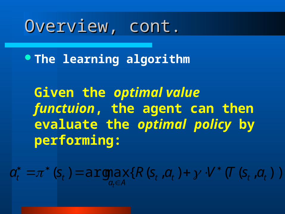
The learning algorithm

Uses experiences to progressively learn the optimal value function, which is the function that predicts the best long term outcome an agent could receive from a given state



The agent studies the optimal value function by continually exercising the current, non-optimal estimate of the value function and improving this estimate after every experience



Given the optimal value functuion, the agent can then evaluate the optimal policy by performing:

))},((),({maxarg)( ttttAa

tt asTVasRsat

DescriptionDescription

Overviewed the field of Learning in general and focused on RL algorithms

Implemented various RL algorithms on a chosen task, aiming to teach the agent the best way to perform the task

Description, cont.Description, cont.

The task of the agentGiven a car’s initial location

and velocity, bring it to a desired location with a zero velocity, as quickly as possible !


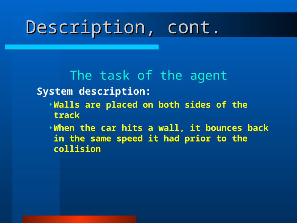
The task of the agentSystem description:

• The car can move either forward or backwards

• The agent can control the car’s acceleration at any time interval


The task of the agentSystem description:

• Walls are placed on both sides of the track• When the car hits a wall, it bounces back in

the same speed it had prior to the collision


A sketch of the system


The code was written using MATLABPerformed experiments to determine the

influence of different parameters on the Learning algorithm (mainly on convergence and how fast the system studies the optimal policy)

Tested the performance of CMAC as a function approximator (tested for both 1D and 2D functions)

Implementation issuesImplementation issues

Function approximators - Representing the Value/Q Function– Lookup Tables

• A finite ordered set of elements (A possible implementation would be an array). Each element is uniquely associated with an index. Accessing the element would be through it’s index.

• Each region in a continuous state space is mapped into an element of the lookup table. Thus, all states within a region are aggregated (accumulated) into one table element, therefore assigned the same value.

Implementation issues, cont.Implementation issues, cont.

Function approximators - Representing the Value/Q Function– Lookup Tables

• This mapping from the state space to the Lookup Table can be uniform or non-uniform.

An example of a uniform mapping of the state space to cells


Function approximators - Representing the Value/Q Function– Cerebellar Model Articulation Controller – CMAC

• each state activates a specific set of memory locations (features). The arithmetic sum of their values is the value of the stored function.

A CMAC structure realization


Learning the optimal Value Function

We wish to study the optimal Value Function from which we can deduce the optimal action policy



Our learning algorithm was based on methods of Temporal Difference or shortly, TD



We define the temporal difference as:

)(ˆ)(ˆ))(,()( 1 ttttttt sVsVssRs



At each time step we update the estimated Value Function by calculating:

)()(ˆ)(ˆ1 ttttt ssVsV



By definition, the optimal policy satisfies:

))},((),({maxarg)( ttttAa

tt asTVasRsat


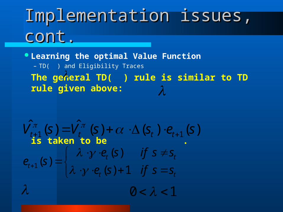
Learning the optimal Value Function– TD( ) and Eligibility Traces

The TD rule as presented above is really an instance of a more general class of algorithms called TD( ) with .

0


Learning the optimal Value Function– TD( ) and Eligibility Traces

The general TD( ) rule is similar to TD rule given above:

is taken to be .

)()()(ˆ)(ˆ11 sessVsV tttt

tt

ttt ssifse

ssifsese

1)(

)()(1

10


Look-Up Table Implementation

– We used a Look-Up Table to represent the Value Function, and acquired the optimal policy by applying the TD( ) algorithm.

– We used a non uniform mapping of the state space to cells in the Look-Up Table which enabled us to keep a rather small number of cells but still have a fine quantization around the origin.


CMAC Implementation - 1

– CMAC is used to represent the Value Function and TD( ) is the learning algorithm.

CMAC Implementation - 2

– CMAC is used to represent the Q-Function and TD( ) is the learning algorithm.


System simulation description

We simulated each of the three implementations for different values of .

For each value of we tested the system for different values of

. was taken to be 1 throughout the simulations.

9.0,5.0,0

8.0,5.0,2.0

Simulation ResultsSimulation Results

We define:– success rate:

The percentage of all tries in which the agent has successfuly been able to bring the car to it’s destination with zero velocity


We define:– Average way:

The average of the time intervals it took the agent to bring the car to it’s destination


Look-Up Table results– A common result for all parameter variants is the improvement

of the success rate and the shortening of the average way to goal as learning progresses.

– For a given , it’s hard to observe any differences between the results for different values of .

– As increases, the learning process is better i.e. For a given try number, the results for the success rate and average way are better.


Look-Up Table results– It’s noted that eventually, in all cases, the success

rate reaches 100% i.e. the agent successfully brought the car to it’s goal.

Look-Up Table performance summary


CMAC Q-Function results– A common result for all parameter variants is the

improvement of the success rate and the shortening of the average way to goal as learning progresses.

– For a given , better results were obtained for a bigger .

– As increases, the learning process is generally better.


CMAC Q-Function results– In most cases, 100% success rate is not reached,

though it reaches 100% in some cases.– We can see in some cases that the success rate

decreases along the tries and increases again.

CMAC Q-Learning performance summary


CMAC Value Iteration results– The figure ahead shows the results obtained by

CMAC Value Iteration implementation compared to the results already obtained for the CMAC Q-Learning implementation. The results are for the best pair of ( ) as obtained from previous results.

,


CMAC Value Iteration results

A comparison between CMAC Q-Learning and CMAC Value Iteration performance


Learning process examples– In figure 1 we show the process of learning for a

specific starting state and learning parameters. The figure shows the movement of the car after every few tries, for 150 time consecutive time intervals.

– In figure 2 we demonstrate the systems ability (at the end of learning) to direct the car to it’s goal starting from different states.

Figure 1: The progress of learning for: 2.0,2.0 ,9.0 ,8.0 0 s

Figure 2: The systems performance from different starting states after try 20 with the

parameters: 9.0 ,8.0

ConclusionsConclusions

In this project we implemented a family of R.L. Algorithms, , with two different function approximators, CMAC and Look-Up Table.

)(TD


We examined the affect of the learning parameters, , and on the overall performance of the system.– In the Look-Up Table implementation: does not

have a significant impact on the results; as increases the success rate increases more rapidly.


We examined the affect of the learning parameters, , and on the overall performance of the system.– In the CMAC implementation: as or

increases, the success rate increases and the average way decreases more rapidly.

reinforcement learning rafy michaeli assaf naor supervisor: yaakov engel visit project’s home page...

Documents

action value function

given state slide

task slide

optimal value function

final state slide

experience slide

action space slide

q function