removal of particulate fines from organic solvents … · ii removal of particulate fines from...
TRANSCRIPT

Removal of Particulate Fines from Organic Solvents Using Water as Collector Droplets
By
SHASHI MALLADI
A thesis submitted in conformity with the requirements for the degree of Master of Applied Science
Department of Chemical Engineering and Applied Chemistry University of Toronto
© Copyright by Shashi Malladi, 2015

ii
Removal of Particulate Fines from Organic Solvents Using Water as Collector Droplets
Shashi Malladi
Master of Applied Science
Department of Chemical Engineering and Applied Chemistry
University of Toronto, 2015
Abstract
A PDMS-based microfluidic aspiration device was developed to carry out a systematic
study of the capture of particles suspended in an organic liquid by using water as collector droplets.
By applying a suitably strong negative pressure at one of the inputs relative to the port delivering
the particles, a water drop was trapped at the constriction and then head-on and glancing collisions
were implemented. Simulations were performed to obtain a measure of particle interaction time
with the drop surface. The relationship between particle capture efficiency and velocity and radius
of the collector droplets was mapped out.
This work aims to provide insight into the feasibility of the use of an aqueous phase for
collecting and separating fines from bitumen- solvent mixture by obtaining statistical data for
particle - drop impingement process. Removal of fines using a water drop is much more energy
efficient than the traditional methods.

iii
Acknowledgements
I would like to express my heart-felt gratitude to my supervisor and mentor, Professor.
Arun Ramachandran, for his belief in me and providing me an opportunity to work under his
esteemed guidance. Without his constant support and encouragement, this would not have been
possible. His enthusiasm and dedication for research has constantly inspired me to perform better
in the field of research. Frequent discussions with him during the course of two years has helped
me widen my mental horizon. I would also like to thank Prof. Edgar Acosta and Prof. Eugenia
Kumacheva for granting me permission to use equipment in their lab.
A special word of thanks to my labmates Dr. Thomas Leary, Yang Li, Suraj Borkar, Rohit
Sonthalia, Sachin Goel, Ghata Nirmal and Dinesh Kumar for their valuable inputs and support. I
would also like to thank Ali Hussain Motagamwala for his help when I was new to the lab. I would
also like to thank Gabriella Lestari, Mokit Chau and William Wang for their help.
I sincerely thank my parents, Muralidhar and Janaki Malladi, and my brother for allowing
me to follow my dreams and believing in me. Without their encouragement, immense patience and
unconditional love, I would not have been able to achieve this. A special word of thanks to my
friends for their constant support. I would also like to acknowledge ACS PRF for funding my
research.
-Shashi Malladi
iv
Table of Contents
List of Tables ................................................................................................................................. vi
List of Figures ............................................................................................................................... vii
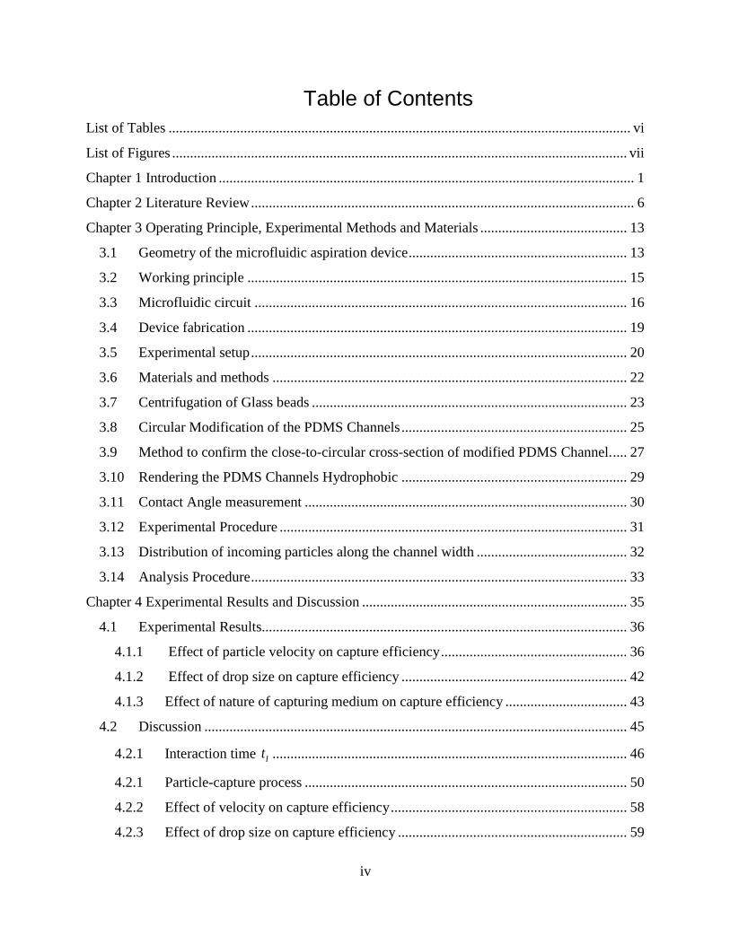
Chapter 1 Introduction .................................................................................................................... 1
Chapter 2 Literature Review ........................................................................................................... 6
Chapter 3 Operating Principle, Experimental Methods and Materials ......................................... 13
3.1 Geometry of the microfluidic aspiration device ............................................................. 13
3.2 Working principle .......................................................................................................... 15
3.3 Microfluidic circuit ........................................................................................................ 16
3.4 Device fabrication .......................................................................................................... 19
3.5 Experimental setup ......................................................................................................... 20
3.6 Materials and methods ................................................................................................... 22
3.7 Centrifugation of Glass beads ........................................................................................ 23
3.8 Circular Modification of the PDMS Channels ............................................................... 25
3.9 Method to confirm the close-to-circular cross-section of modified PDMS Channel. .... 27
3.10 Rendering the PDMS Channels Hydrophobic ............................................................... 29
3.11 Contact Angle measurement .......................................................................................... 30
3.12 Experimental Procedure ................................................................................................. 31
3.13 Distribution of incoming particles along the channel width .......................................... 32
3.14 Analysis Procedure ......................................................................................................... 33
Chapter 4 Experimental Results and Discussion .......................................................................... 35
4.1 Experimental Results...................................................................................................... 36
4.1.1 Effect of particle velocity on capture efficiency .................................................... 36
4.1.2 Effect of drop size on capture efficiency ............................................................... 42
4.1.3 Effect of nature of capturing medium on capture efficiency .................................. 43
4.2 Discussion ...................................................................................................................... 45
4.2.1 Interaction time It ................................................................................................... 46
4.2.1 Particle-capture process .......................................................................................... 50
4.2.2 Effect of velocity on capture efficiency .................................................................. 58
4.2.3 Effect of drop size on capture efficiency ................................................................ 59

v
4.2.4 Effect of nature of capturing medium on capture efficiency .................................. 60
Chapter 5 Conclusions and Future Work ...................................................................................... 61
5.1 Conclusions .................................................................................................................... 61
5.2 Future Work ................................................................................................................... 63
5.2.1 Better focusing via additional junctions ................................................................. 63
5.2.2 Experiments for confirmation of bridge formation model ...................................... 63
5.2.3 Alternative design for the microfluidic aspiration device ....................................... 64
5.2.4 Coalescence of two soft particles ............................................................................ 65
5.2.5 Compatibility with the material of construction ..................................................... 66
References ..................................................................................................................................... 68
Appendix A ................................................................................................................................... 76
Appendix B ................................................................................................................................... 78
Appendix C ................................................................................................................................... 82
C.1 Derivation for Hydrodynamic Film Drainage ................................................................ 82
C.2 Energy requirement for Bridge Formation Theory ........................................................ 84
Contribution .................................................................................................................................. 86

vi
List of Tables
Table 1. Experimental matrix for study of effect of nature of capturing medium on particle capture
process........................................................................................................................................... 44

vii
List of Figures
Figure 1.1. Oil sands model proposed by J. H. Cottrell (Picture taken from K.A. Clark volume
[13]).
Figure 1.2. Schematic of the non-aqueous bitumen extraction process.
Figure 2.1. Steps in particle-capture process. a) Film drainage, b) Instability of the film, c) Bridge
Formation /Attachment, d) Penetration, e) Engulfment.
Figure 2.2. Sequence of interface shapes zoomed in near the interface for a particle penetrating
into an interface at Ca = 1 for*
H,effA =0.0531 . Time, t, is normalized as2
ptF R . The co-
ordinates are rendered dimensionless by the drop radius, and the particle is 1/100 that of the drop.
(Image taken from simulations done by Dr. Thomas Leary).
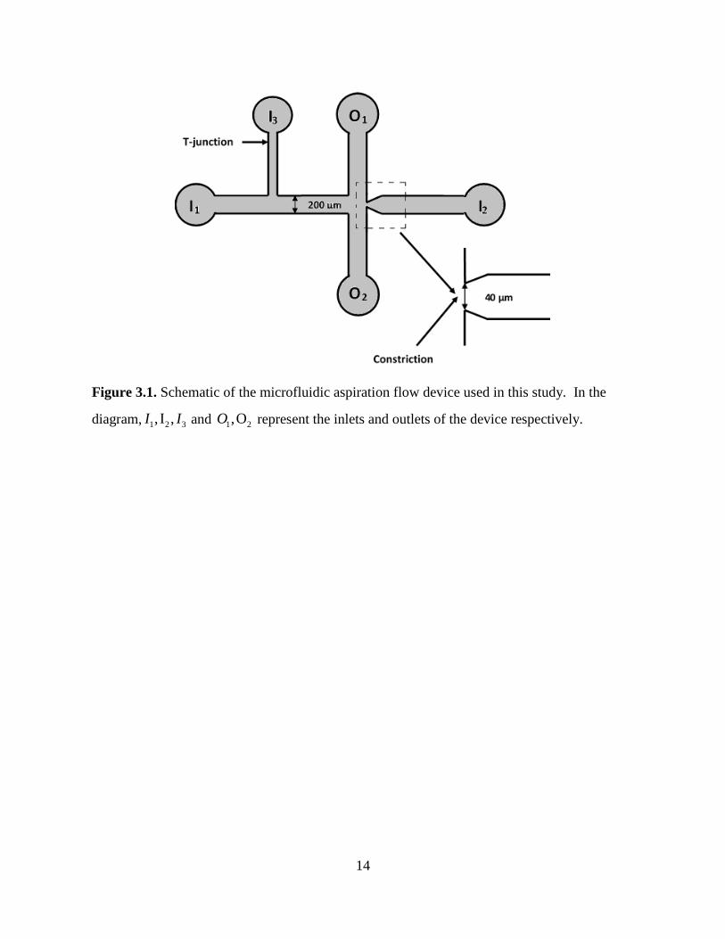
Figure 3.1. Schematic of the microfluidic aspiration flow device used in this study. In the diagram,
1 2 3, I ,I I and 1 2,OO represent the inlets and outlets of the device respectively.
Figure 3.2. Geometric specification of the microfluidic aspiration device.
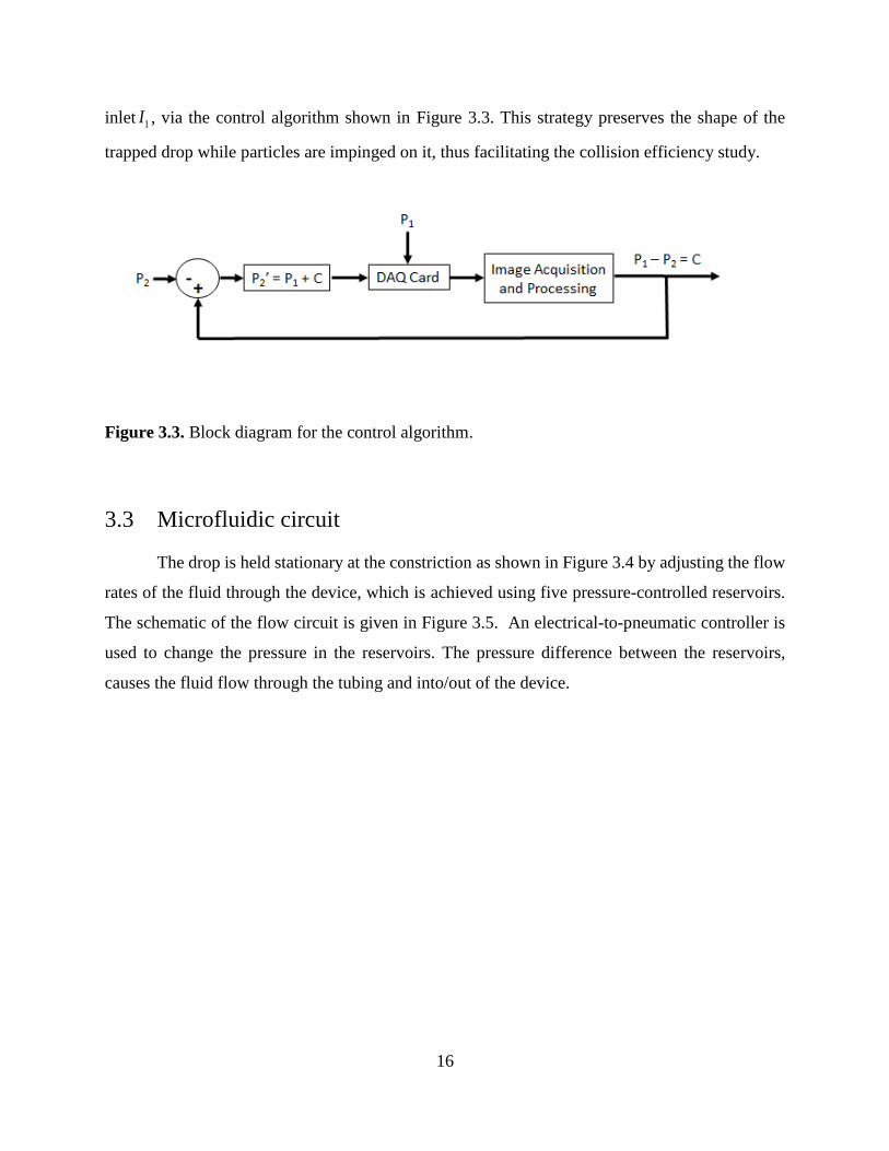
Figure 3.3. Block diagram for the control algorithm.
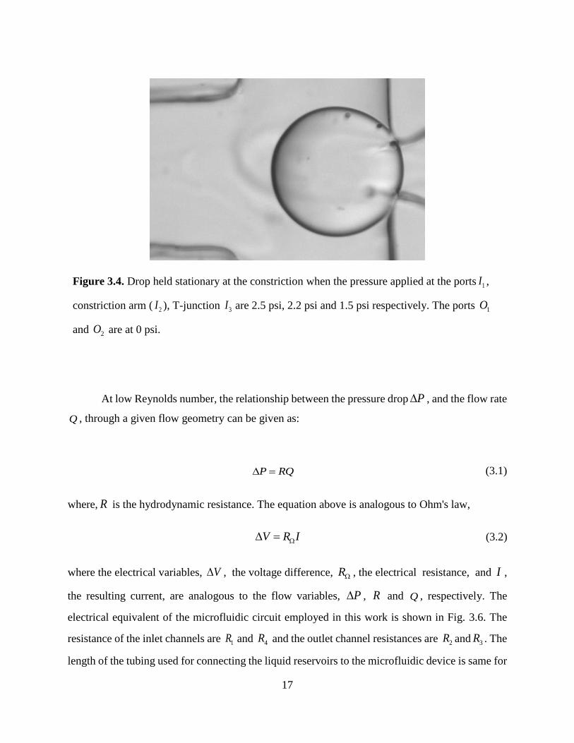
Figure 3.4. Drop held stationary at the constriction when the pressure applied at the ports 1I ,
constriction arm ( 2I ), T-junction 3I are 2.5 psi, 2.2 psi and 1.5 psi respectively. The ports 1O and
2O are at 0 psi.
Figure 3.5. Schematic of the flow device and connection to the fluid reservoirs. 1 2 3 4, ,R ,RR R and
5R are the hydrodynamic resistances of each arm of the microfluidic device and '
1R , '
2R , '
3R '
4R and
'
5R are the hydrodynamic resistances of the external circular tubing.
Figure 3.6. Electrical representation of microfluidic channel. 1 2 3, ,P P P and 4P are the pressure in
the reservoirs. 1 2 3,Q ,QQ and 4Q are the flow rates through each arm.
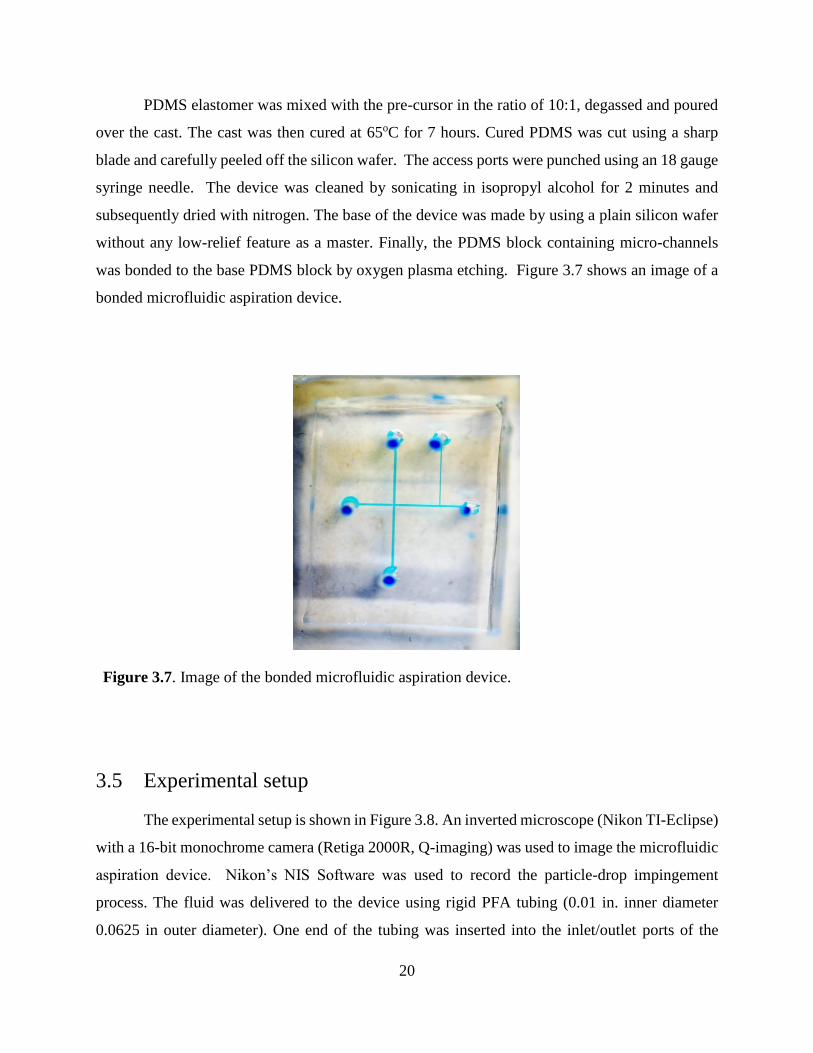
Figure 3.7. Image of the bonded microfluidic aspiration device.
Figure 3.8. Schematic of the experimental setup.
Figure 3.9. Size distribution of glass beads after centrifugation.
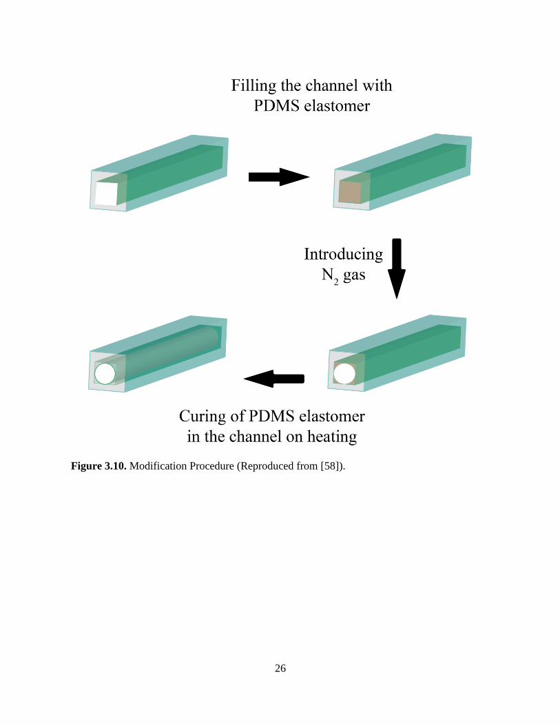
Figure 3.10. Modification Procedure (Reproduced from [58]).
Figure 3.11. Rectangular cross-section of the channel-at-large obtained by 3D reconstruction of
21 images.
Figure 3.12. Modified cross-section of the channel-at-large obtained by 3D reconstruction of 21
images.

viii
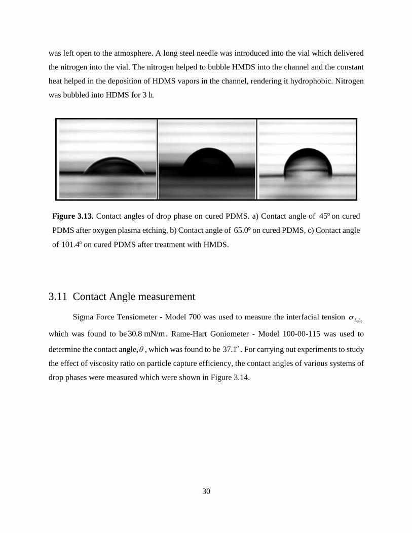
Figure 3.13. Contact angles of drop phase on cured PDMS. a) Contact angle of 45on cured
PDMS after oxygen plasma etching, b) Contact angle of 65.0on cured PDMS, c) Contact angle
of 101.4on cured PDMS after treatment with HMDS.
Figure 3.14. Contact angles in mineral oil. a) DI water on glass 25.4 , b) Glycerol/DI water
mixture on glass 35.1 , c) Glycerol/IPA mixture on glass 65.4 .
Figure 3.15. Fraction of particles entering the channel along 100y m at z = 0 at a velocity
of 0.718 mm/s.
Figure 3.16. Block diagram of multiple particle - tracking algorithm.
Figure 4.1.Variation of y within the limiting ordinates.
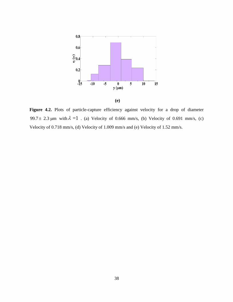
Figure 4.2. Plots of particle-capture efficiency against velocity for a drop of diameter
99.7 2.3 μm with =1 . (a) Velocity of 0.666 mm/s, (b) Velocity of 0.691 mm/s, (c) Velocity
of 0.718 mm/s, (d) Velocity of 1.009 mm/s and (e) Velocity of 1.52 mm/s.
Figure 4.3. Plot of capture efficiency against applied velocity for a drop of diameter
99.7 2.3 μm with =1 at mid-plane (z = 0) and y between ± 10 µm from device center (y =
0).
Figure 4.4. Plot of capture efficiency against the total time elapsed for a velocity of 1 mm/s for a
drop diameter of 100 μm with = 1 .
Figure 4.5. Plot of capture efficiency against y for different time intervals for a velocity of 1 mm/s,
drop diameter of 100 µm with λ=1. (a) Time = 7 mins, (b) Time = 14 mins (next 7 mins of the
experiment), (c) Time = 21 mins (next 7 mins of the experiment) and (d) Time = 28 mins (next 7
mins of the experiment).
Figure 4.6. Plots of capture efficiency against drop size for a velocity of 1.52 mm/s and 1 . (a)
Drop of 52 µm, (b) Drop of 79.5 µm, (c) Drop of 84.1 µm and (d) Drop of 100 µm.
Figure 4.7. Plot of capture efficiency against drop diameter for a velocity of 1.52 mm/s and 1
at mid-plane (z = 0) and y between ± 10 µm from device center (y = 0).
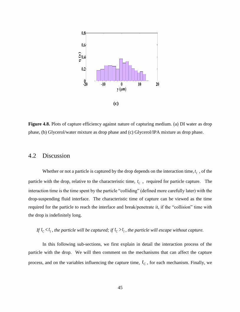
Figure 4.8. Plots of capture efficiency against nature of capturing medium. (a) DI water as drop
phase, (b) Glycerol/water mixture as drop phase and (c) Glycerol/IPA mixture as drop phase.
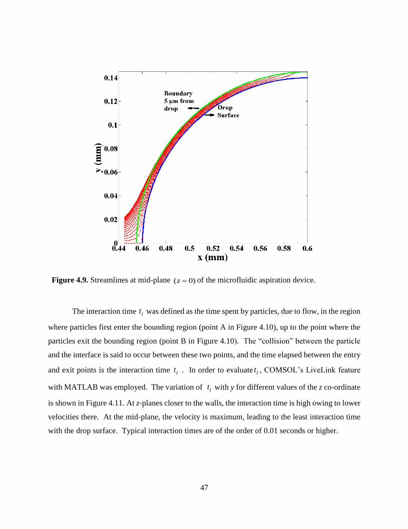
Figure 4.9. Streamlines at mid-plane ( 0)z of the microfluidic aspiration device.
Figure 4.10. Streamline within the bounding region. The region between point A and C is the
approach phase and the region between point C and B is the separation phase.
Figure 4.11. Plot of total interaction time of particle within the bounding region along
100y m the device width for different Z-planes z = ± 50 μm .

ix
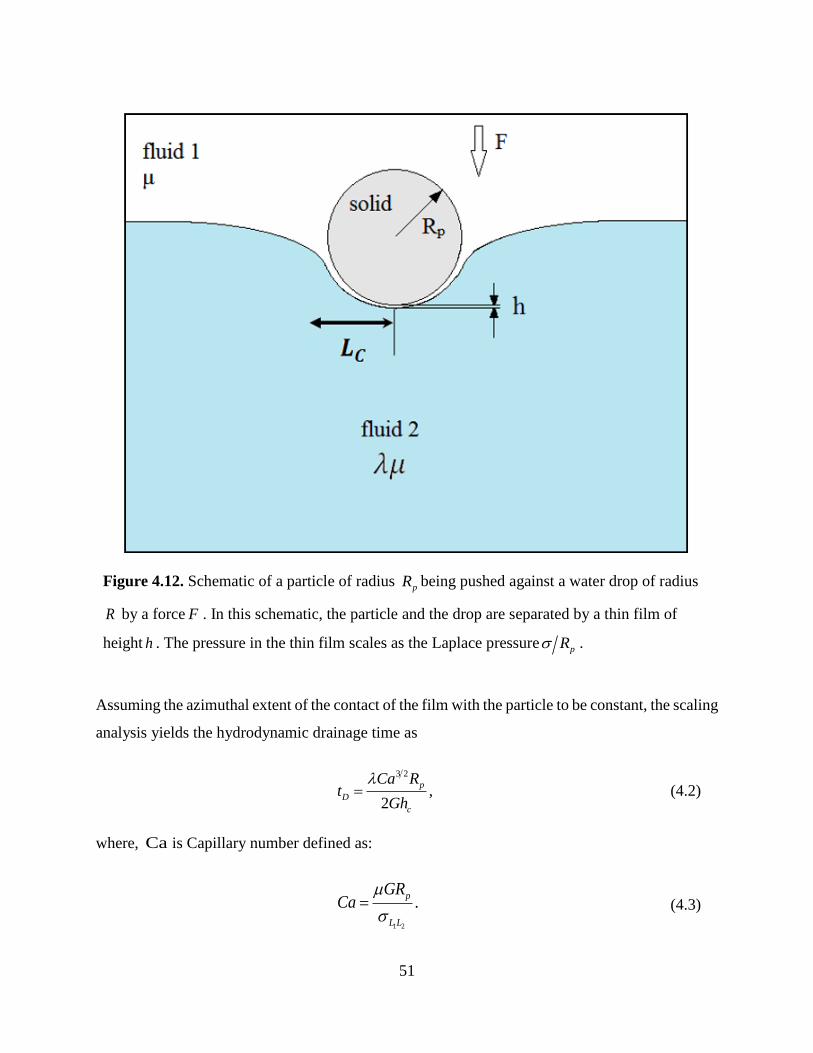
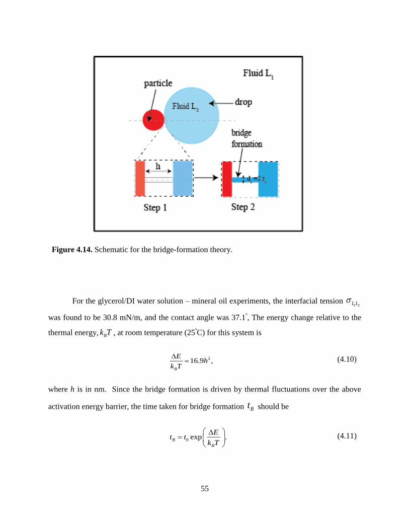
Figure 4.12. Schematic of a particle of radius pR being pushed against a water drop of radius R
by a force F . In this schematic, the particle and the drop are separated by a thin film of height h .
The pressure in the thin film scales as the Laplace pressurepR .
Figure 4.13. Forces acting on a particle attached to the interface along with the motion of the
contact line.
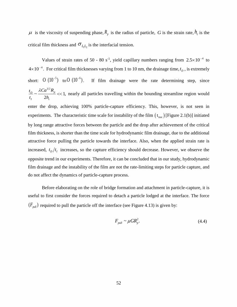
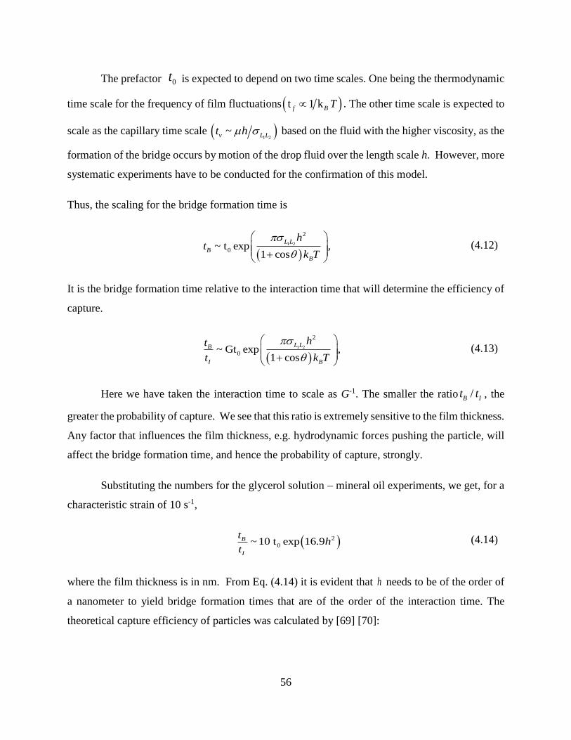
Figure 4.14. Schematic for the bridge-formation theory.
Figure 4.15. Capture Efficiency as a function of film thickness h .
Figure 4.16. Plot of capture efficiency as a function of strain rate (1/s).
Figure 5.1. Modified design for enhanced focussing of particles
Figure 5.2. Drop held at the tip of a silica capillary in the microfluidic aspiration device (Image
taken from Rohit Sonthalia).
Figure 5.3. Drop Coalescence in the microfluidic aspiration device (Image taken from Rohit
Sonthalia).
Figure 5.4. Glass-based microfluidic aspiration device (Image taken from Rohit Sonthalia).

1
Chapter 1 Introduction
Oil Sands, an unconventional petroleum reserve that is widely found in the Athabasca belt
of Canada [1] [2] are an important natural resource and a profitable alternative when the price of
oil is more than about $60 per barrel [3]. In 2005, the Canadian Energy Research Institute (CERI)
estimated that over the period 2000-2020, oil sands and oil sands-related activities together could
contribute around $789 billion to Canada’s GDP [4]. The typical composition of oil sands is around
4-18 wt. % bitumen, 55-80 wt. % sands, fine solids (particles < 44 µm (5-34 wt. %)) and around
2-15 wt. % water [5]. Surface Mining and in-situ methods such as SAGD (Steam Assisted Gravity
Drainage) method [6], VAPEX (Vapor Extraction) [7], THAI (Toe to Heel Air Injection) [8], CSS
(Cyclic Steam Simulation) [9] are the conventional methods adopted for extracting bitumen from
oil sands. These methods require around 17 to 21 barrels of freshwater per barrel of oil produced
from oil sands [10]. The strong electrostatic forces between the adhered fines, reduces the settling
of fines. Continuous accumulation of low viscosity sludge and slow compaction and settling
require vast acres of tailing ponds which were reported to be around 50 square kilometers in 2006
[11] [12]. Thus, the environmental impact of excess usage of water and land, associated with the
conventional methods, has led to the exploration of environment-friendly alternative processes in
the recent years.

2
Figure 1.1. Oil sands model proposed by J. H. Cottrell (Picture taken from K.A. Clark volume
[13]).
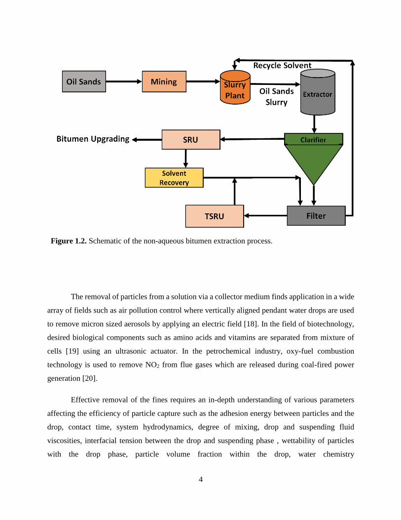
The non-aqueous process of extraction [14] of bitumen from oil sands, shown in Figure
1.2, is a relatively new initiative in the area of oil-sands extraction, driven by the need to reduce
the requirement of fresh water in the extraction process. The process involves mining of the oil
sands and introducing the crushed ore into the slurry plant where it is mixed with a solvent like
heptane or toluene to help separate bitumen from the sand particles. The slurry is transported to
the extractor and the clarifier for the removal of the solid particulates and suspended solids from
the bitumen-solvent mixture. The sludge collected from the bottom of the clarifier is sent through
a filter to separate the solid particles from the solvent. The solvent recovered from SRU (Solvent

3
Recovery Unit) and TSRU (Tailings Solvent Recovery Unit) is resent through filters and finally
the solvent is recycled into the slurry plant. The bitumen-solvent mixture from the clarifier is sent
to the SRU where the solvent is recovered and bitumen is sent to the upgrading units. During the
bitumen extraction process, significant amounts of particulate fines are extracted along with the
bitumen [15].
Removal of these fines is necessary as they reduce the bitumen recovery from oil sands by
altering the water chemistry [16]. The fines clog the catalyst pellets and filters in the upgrading
units leading to a reduction in the efficiency of the equipment eventually leading to its premature
failure. Though the coarse particulates in the mixture of solvent and sands can be removed by
inclined settlers, they have proved to be ineffective for the removal of micron and sub-micron
sized particles [11]. Also current methods like centrifugation and solvent evaporation employed
for the removal of these particles are energy intensive and possess potential hazards of emissions.
It is known that clays [11], the major component of the fine particulates in oil sands, are naturally
water wetting [17]. This suggests a possible route for the separation of these fines from the
bitumen-solvent organic phase by mixing the particle-solvent suspension with water. When the
solvent-particle-water mixture is agitated, the water droplets serve as collectors for the particles
via penetration through the solvent-water interface facilitated by their wettability. The collector
droplets can then be separated by gravity much more easily relative to the individual particles
owing to their larger sizes.
4
Figure 1.2. Schematic of the non-aqueous bitumen extraction process.
The removal of particles from a solution via a collector medium finds application in a wide
array of fields such as air pollution control where vertically aligned pendant water drops are used
to remove micron sized aerosols by applying an electric field [18]. In the field of biotechnology,
desired biological components such as amino acids and vitamins are separated from mixture of
cells [19] using an ultrasonic actuator. In the petrochemical industry, oxy-fuel combustion
technology is used to remove NO2 from flue gases which are released during coal-fired power
generation [20].
Effective removal of the fines requires an in-depth understanding of various parameters
affecting the efficiency of particle capture such as the adhesion energy between particles and the
drop, contact time, system hydrodynamics, degree of mixing, drop and suspending fluid
viscosities, interfacial tension between the drop and suspending phase , wettability of particles
with the drop phase, particle volume fraction within the drop, water chemistry

5
(surfactant/polymer/salt concentrations and pH) and affinity of the particles to the suspending
medium [21]. This emphasizes the need for a detailed and fundamental study of particle-drop
collision dynamics.
The primary objective of this work is to obtain statistical data for particle - drop
impingement process and to provide insight into the feasibility of the use of an aqueous phase for
collecting and separating fines from the solvent-particle mixture. For our experiments,
hydrodynamic forces were used to direct a suspension of hollow glass beads in mineral oil towards
a stationary drop. A PDMS-based microfluidic aspiration device, was developed to carry out drop-
particle interaction experiments. Glycerol/water drops were generated at the T-junction and one
drop was held at the constriction. The particle-capture events were recorded using an inverted
microscope and a CCD camera. Images were analyzed by implementing custom-designed particle
tracking algorithms in MATLAB. Parameters such as velocity and droplet size were changed to
study their effect on collision efficiency.
This work is organised as follows: The literature review of the importance of removal of
the particulates fines and the current removal methods have been detailed in Chapter 2. Chapter 3
discusses the design of the microfluidic aspiration device, its working principle, the experimental
materials and methods and the control algorithm used to track particle trajectory. Our experimental
results and discussions, formulates Chapter 4. Finally, in Chapter 5, our conclusion and the future
work has been discussed.

6
Chapter 2 Literature Review
A major utility of an understanding of particle-drop collision dynamics is in the systematic
design of separators for removing particulate fines in complex mixtures. Bitumen obtained from
oils sands using solvent extraction, contains a considerable amount of fine particles depending on
the quality of the feed stock and the extracting solvent-feed contact methods [21]. The removal of
these fines is crucial for the optimal performance of different refinery vessels. Tu and co-workers
[22] in one of their studies determined that sub-micron sized particles prevent bitumen froth
formation by increasing the viscosity of bitumen slurry, thus hindering the performance of primary
separation vessels (PSVs). Wang et al. [23] proved that during the hydrotreating process, kaolinite
fines deposit on the catalyst pellets of packed-bed reactors, which in turn causes a huge pressure
drop in the reactor and lowers the conversion efficiency, leading to premature reactor shutdown.
These studies hint at the necessity for removal of particulate fines before upgrading bitumen into
lighter oil fractions.
Efforts have been made by Rubio et al. for the removal of the hydrophobic fines by using
a hydrophobic polymer carrier like polypropylene. The fines stick onto the surface of the polymer
via hydrophobic interactions [24]. However, this method involves the introduction of a polymeric
material into the suspension for separation of the fines. The additional task of polymer recovery
makes this process expensive and energy-intensive. Another strategy used by researchers was the
formation of particle flocs or agglomerates followed by gravity induced separation [21]. The
particle agglomeration process necessitates the addition of large concentrations of surface-active
wetting compounds such as catechol, resorcinol and formic acids to the suspension for separation
of the fines. Addition of large quantities of chemicals is not economically viable. Warren reported
the use of shear field for inducing particle flocculation [25]. The idea of particle-suspension
instability by the application of shear field and the presence of surfactants leading to particle
agglomeration was used by Li et al [26]. In all these studies, experiments were conducted at a
macroscopic scale, without paying heed to the processes at a microscopic/fundamental level.
Recent years have seen the gaining prominence of the bottom-up approach [27] [28] [29],
whereby the behaviour of few particles at micro-scale are studied, both theoretically and
7
experimentally, and the findings are extended to understand behaviour in more concentrated
suspensions. Mixtures of particulate suspensions and emulsions find tremendous application, in a
variety of industries including petroleum [30], cosmetic, paint, detergent/fabric enhancer [31],
pharmaceutical [32], and polymer industry [33]. However, the behaviour of these complex fluids
under various formulations are not fully understood. The lack of a more fundamental
understanding and characterisation of these suspensions has posed industrial losses resulting from
improper product properties and function. Study of emulsions using the bottom-up approach
provides a better understanding of the behaviour and the structure-property relationship of these
suspensions, thus, overcoming the problems of low shelf-life and poor functionality. However,
there has been limited work done in understanding the properties of multicomponent mixtures of
particulates and drops via the study of a single particle-drop interaction.
Research attempts at describing such interactions at a microscopic level have been majorly
directed towards establishing the effect of relative tension between the three phases, namely the
rigid particles and the two liquid phases, on the equilibrium properties of these mixtures. As
discussed by Niven et al. [34], for a case of a preferentially wetting dispersed phase, a liquid bridge
(capillary bridge) between the particles is formed and prevalence of strong attractive forces leads
to particulate agglomeration. On the other hand, when the dispersed phase is non-wetting, capillary
repulsive forces acting on the particles push them outwards, until a globular mixed particle
configuration is assumed wherein particles arrange themselves at the interface between the droplet
and the suspending medium. These equilibrium properties are described in terms of the interplay
between the work of adhesion and cohesion. Furthermore, energetic models based on Gibbs free
energy have been developed for the stability and rupture mechanisms of these globular mixed
particles. Niven et al. also showed that when the dispersed phase is preferentially non wetting, an
isolated solid particle requires least energy for its detachment from the drop interface. With an
increase in the available energy, one by one all particles leave their n-plet configuration (n rigid
particles at the interface between the drop and suspending fluid) and eventually the drop surface
is devoid of solid particles. These energetics were then used to predict the size distribution of
globular particles in turbulent flow regimes [34] [35] by analyzing the available energy for
breakup. While these energetic models help in deducing the evolution of particle mixed phase,
there is a need to also understand the dynamics of formation of these globular clusters by the

8
collision of particles with the dispersed phase. A fundamental knowledge of the dynamics of
particle-drop collisions is, thus, needed to determine the particle collection efficiency of drops.
This project is motivated by the possibility of removal of clay particles by entrapping them
in water drops. Since clay particles in the Athabasca oil sands are inherently hydrophilic, they have
strong affinity towards water, making it possible to incorporate our work for particulate removal
[36] in the petroleum industry. However, the carboxylates, asphaltenes and naphthenic
components [37] [38] [39] [40] adsorbed on the surface of clay particles alter its wettability making
the surface partly hydrophobic and partly hydrophilic, thus preventing them from crossing the
interface and entering the drop. The interfacial tension of bitumen/water mixture of around 36.4
mN/m [41] and the chemical species released from bitumen [42] causes the latter to stick firmly
to the clay particles.
The particle-drop collision capture process is strongly dependent on the particle-drop
interaction time, film drainage time, wettability of particles with the drop phase and the surface
energy. The various steps involved in a particle-drop collision capture process are hydrodynamic
film drainage leading to instability of the film, bridge formation, attachment, penetration of particle
by motion of the contact line around the particle and eventually engulfment of the particle by the
water drop. Since the particle separation technique involves the impingement of particles on
stationary water droplets and capturing them by producing a new particle-water interface, it is
important to understand the mechanism of this process.
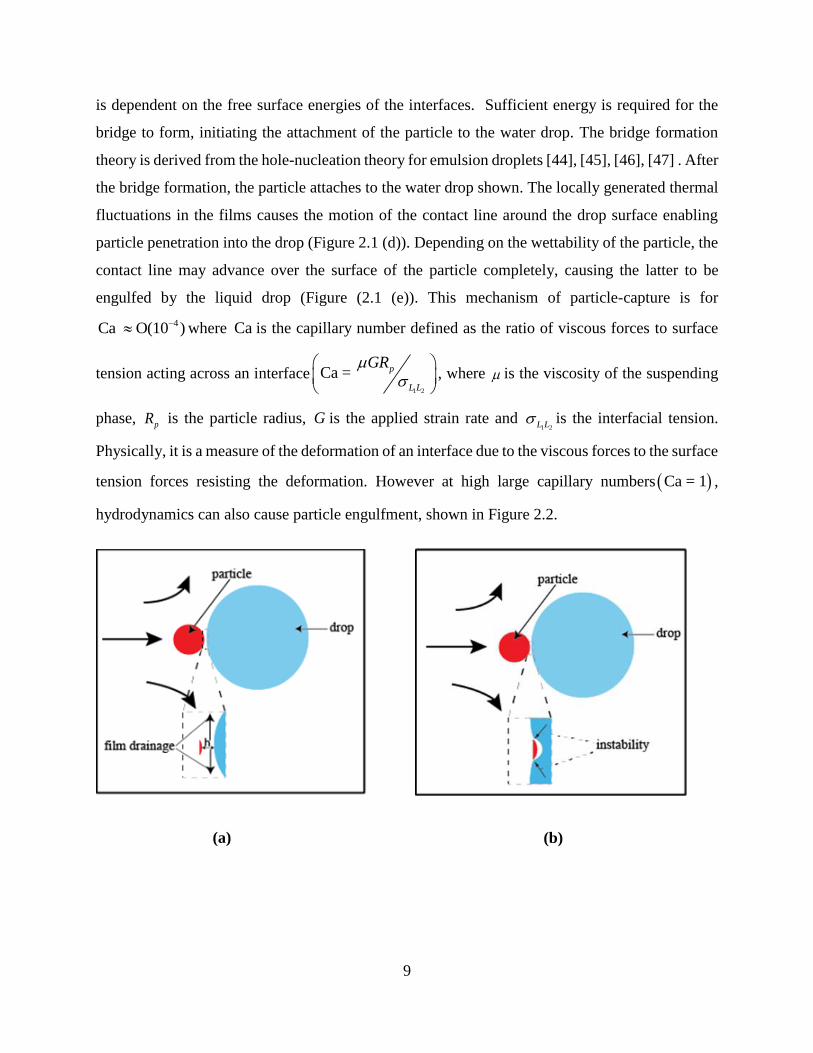
The penetration of particle into a water drop in a head-on collision configuration
presumably occurs by the mechanism depicted in Figure 2.1. When a particle, moving through a
viscous fluid, is pushed against a stationary water drop by a force F , the effect of fluid film
drainage between the particle and drop and the viscous dissipation of energy causes the
deformation of the fluid interface [43]. This is called hydrodynamic film drainage phase shown
in Figure 2.1 (a). The particle deforms the fluid interface until a critical film thickness is reached.
Here, attractive forces like van der Waals force sets in, which has a destabilizing effect on the film
(see Figure 2.1 (b)), leading to the increase in the disjoining pressure in the film, causing the
rupture of the intervening film in between the drop and the particle. Eventually a bridge is formed
between the drop and particle shown in Figure 2.1 (c). The energy required for the bridge formation
9
is dependent on the free surface energies of the interfaces. Sufficient energy is required for the
bridge to form, initiating the attachment of the particle to the water drop. The bridge formation
theory is derived from the hole-nucleation theory for emulsion droplets [44], [45], [46], [47] . After
the bridge formation, the particle attaches to the water drop shown. The locally generated thermal
fluctuations in the films causes the motion of the contact line around the drop surface enabling
particle penetration into the drop (Figure 2.1 (d)). Depending on the wettability of the particle, the
contact line may advance over the surface of the particle completely, causing the latter to be
engulfed by the liquid drop (Figure (2.1 (e)). This mechanism of particle-capture is for
4Ca O(10 ) where Ca is the capillary number defined as the ratio of viscous forces to surface
tension acting across an interface1 2
Ca = p
L L
GR
, where is the viscosity of the suspending
phase, pR is the particle radius, G is the applied strain rate and
1 2L L is the interfacial tension.
Physically, it is a measure of the deformation of an interface due to the viscous forces to the surface
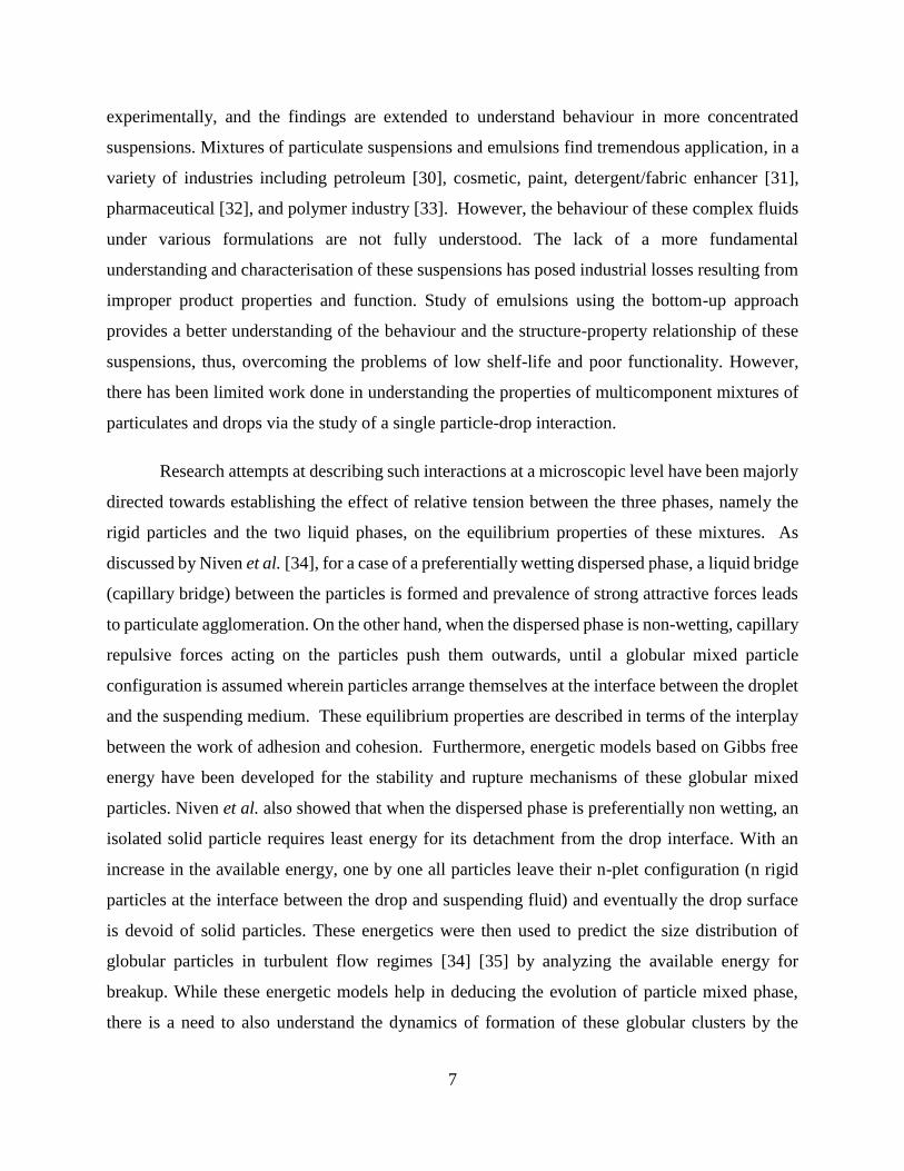
tension forces resisting the deformation. However at high large capillary numbers Ca = 1 ,
hydrodynamics can also cause particle engulfment, shown in Figure 2.2.
(a) (b)

10
Figure 2.1. Steps in particle-capture process. a) Film drainage, b) Instability of the film, c)
Bridge Formation /Attachment, d) Penetration, e) Engulfment.
(c) (d)
(e)

11
Figure 2.2. Sequence of interface shapes zoomed in near the interface for a particle penetrating
into an interface at Ca = 1 for*
H,effA =0.0531 . Time, t, is normalized as2
ptF R . The co-
ordinates are rendered dimensionless by the drop radius, and the particle is 1/100 that of the
drop. (Image taken from simulations done by Dr. Thomas Leary).
Particle capture by a collector medium has been explained in the past using the colloidal
filtration theory (CFT) [48]. This theory was originally developed for waste water filtration
process. The process comprises two steps, one being the transportation of the suspended particles
towards the collector interface by the fluid flow and the second step involves the attachment of the
particle to the interface. Based on the particle size and density relative to the suspending phase, a
particle comes in contact with the collector by transport processes such as interception,
sedimentation or diffusion. The adhesion of particles to the collector depends on the adhesion
forces between the particle and the drop. However, in this theory, the role of hydrodynamic and
van der Waals interactions in the filtration behaviour of colloidal particles were neglected, which
was included in the work of Tufenkji et al [49] . In this work, colloidal particles were impinged
on non-deformable spherical collectors and the overall collector capture efficiency was defined as

12
the ratio of the net particle deposition on the collector to the total number of particles transported
to the projected area of the collector. For particles of order 10 µm, they obtained capture efficiency
of around 20 %.
Effective separation of the fines, emphasizes the need for a systematic study and
understanding of the particle-drop interaction. It is also crucial to determine which of the above
mentioned phenomena are responsible for the fines separation process. To our knowledge, this
work is the first of its kind to carry out a systematic study to characterize particle-drop interaction
dynamics using a flow field.
One way of carrying out a particle-drop impingement study is in a cross-slot or diamond-
shaped device developed by Schroeder and Ali respectively that employ hydrodynamic forces to
trap and manipulate particle positions [50] [51]. The diamond-shaped device developed by Ali can
be used to carry out particle-drop impingement studies. However, this device requires complex
control algorithms to hold the drop stationary at the stagnation point which can be avoided by
using our geometry. The modification of this cross-slot design wherein one of the arms is provided
with a constriction is more applicable. This new design acts like a microfluidic aspiration device
in which the modified arm is used to trap a drop at its constriction. By doing this, the remaining
three arms can be used to maintain a steady flow condition and to direct particles towards the drop.
In our study, the effect of velocity and drop size on particle collection efficiency will be
interrogated.

13
Chapter 3 Operating Principle, Experimental Methods and
Materials
3.1 Geometry of the microfluidic aspiration device
The schematic of the microfluidic aspiration device used in this study, is shown in Figure
3.1. It is a five-port device with three inlets ( 1I , 2I and 3I ) and two outlets ( 1O , 2O ). Each port is
connected to a reservoir, which is pressurized using a pressure transducer. The inlets 1I and 2I are
connected to oil reservoirs, while the inlet 3I is connected to a water reservoir. The channel leading
out of 2I meets at the intersection between the channels from 1I , 1O and 2O via a constriction. The
width and depth of the device channels are 200 µm and 100 µm respectively. The width of the
constriction is 40 µm. The geometric specifications are shown in Figure 3.2 where z = 0 plane
represents the mid-plane of the device and the plane y = 0 is the center plane along the width of
the device.
14
Figure 3.1. Schematic of the microfluidic aspiration flow device used in this study. In the
diagram, 1 2 3, I ,I I and 1 2,OO represent the inlets and outlets of the device respectively.

15
Figure 3.2. Geometric specification of the microfluidic aspiration device.
3.2 Working principle
The experiment is performed in two steps. First, the water drop is formed in-situ at the T-
junction formed by the channels connected to inlets 1I and 3I . The emulsified water droplet is
carried by the suspending fluid towards the intersection. By applying a suitably strong negative
pressure at 3I relative to the inlet pressure at 1I , the droplet can be trapped at the constriction. In
the second step, particles are introduced from inlet 1I and impinged on the trapped drop. The
average velocity of the flowing particles can be modified by varying the inlet pressure at 1I with
respect to the pressure maintained at the outlets 1O and 2O . A difficulty in implementing this is
that if the pressure in inlet 1I is too high, the trapped drop can be pushed completely into the
constriction. This is avoided by dynamically adjusting the pressure in inlet 2I relative to that in
16
inlet 1I , via the control algorithm shown in Figure 3.3. This strategy preserves the shape of the
trapped drop while particles are impinged on it, thus facilitating the collision efficiency study.
Figure 3.3. Block diagram for the control algorithm.
3.3 Microfluidic circuit
The drop is held stationary at the constriction as shown in Figure 3.4 by adjusting the flow
rates of the fluid through the device, which is achieved using five pressure-controlled reservoirs.
The schematic of the flow circuit is given in Figure 3.5. An electrical-to-pneumatic controller is
used to change the pressure in the reservoirs. The pressure difference between the reservoirs,
causes the fluid flow through the tubing and into/out of the device.
17
Figure 3.4. Drop held stationary at the constriction when the pressure applied at the ports 1I ,
constriction arm ( 2I ), T-junction 3I are 2.5 psi, 2.2 psi and 1.5 psi respectively. The ports 1O
and 2O are at 0 psi.
At low Reynolds number, the relationship between the pressure drop P , and the flow rate
Q , through a given flow geometry can be given as:
P RQ (3.1)
where, R is the hydrodynamic resistance. The equation above is analogous to Ohm's law,
V R I (3.2)
where the electrical variables, V , the voltage difference, R , the electrical resistance, and I ,
the resulting current, are analogous to the flow variables, P , R and Q , respectively. The
electrical equivalent of the microfluidic circuit employed in this work is shown in Fig. 3.6. The
resistance of the inlet channels are 1R and 4R and the outlet channel resistances are 2R and 3R . The
length of the tubing used for connecting the liquid reservoirs to the microfluidic device is same for

18
inlets 1I and 3I and the tubing resistances are '
1R and '
4R respectively. The tubing length used for
outlets 1O and 2O is same and their tubing resistances are '
2R and 3
'R respectively i.e. ' '
4 1R R and
' '
2 3R R . The resistance offered by the tubing connected to the fluid reservoirs is chosen such that
' ' ' '
1 2 3 4 1 2 3 4, , , , , ,R R R R R R R R .
Figure 3.5. Schematic of the flow device and connection to the fluid reservoirs. 1 2 3 4, ,R ,RR R
and 5R are the hydrodynamic resistances of each arm of the microfluidic device and '
1R , '
2R ,
'
3R '
4R and '
5R are the hydrodynamic resistances of the external circular tubing.

19
3.4 Device fabrication
Soft lithography method was used to fabricate the microfluidic aspiration device in PDMS.
This method has been extensively reviewed in the literature [52].
The microfluidic channel design was made using AutoCAD 2012, a computer-aided design
and drafting software. The design was printed at a high resolution of 20,000 DPI on a transparency
mask by Pacific Arts and Design, Toronto. To prepare a master, negative photo-resist (SU-8 50)
was spin-coated onto a 3" diameter silicon wafer. The thickness of the spin-coated SU8-50 was
100 m. The wafer was then pre-baked on a hotplate at 95oC for 15 minutes. The transparency
containing the design was used as a photo-mask in contact photolithography using a mask aligner
which had a lamp power of 16 mJ.cm-2.s-1. The spin-coated silicon wafer was exposed to UV light
(365 nm) for 35 seconds. The wafer was then post-baked on a hotplate at 95oC for 10 minutes. The
unexposed photo-resist was removed by dissolving it in SU8 developer, yielding a silicon wafer
with a positive low-relief of photoresist that served as a casting mold for PDMS.
Figure 3.6. Electrical representation of microfluidic channel. 1 2 3, ,P P P and 4P are the pressure
in the reservoirs. 1 2 3,Q ,QQ and 4Q are the flow rates through each arm.
20
PDMS elastomer was mixed with the pre-cursor in the ratio of 10:1, degassed and poured
over the cast. The cast was then cured at 65oC for 7 hours. Cured PDMS was cut using a sharp
blade and carefully peeled off the silicon wafer. The access ports were punched using an 18 gauge
syringe needle. The device was cleaned by sonicating in isopropyl alcohol for 2 minutes and
subsequently dried with nitrogen. The base of the device was made by using a plain silicon wafer
without any low-relief feature as a master. Finally, the PDMS block containing micro-channels
was bonded to the base PDMS block by oxygen plasma etching. Figure 3.7 shows an image of a
bonded microfluidic aspiration device.
Figure 3.7. Image of the bonded microfluidic aspiration device.
3.5 Experimental setup
The experimental setup is shown in Figure 3.8. An inverted microscope (Nikon TI-Eclipse)
with a 16-bit monochrome camera (Retiga 2000R, Q-imaging) was used to image the microfluidic
aspiration device. Nikon’s NIS Software was used to record the particle-drop impingement
process. The fluid was delivered to the device using rigid PFA tubing (0.01 in. inner diameter
0.0625 in outer diameter). One end of the tubing was inserted into the inlet/outlet ports of the
21
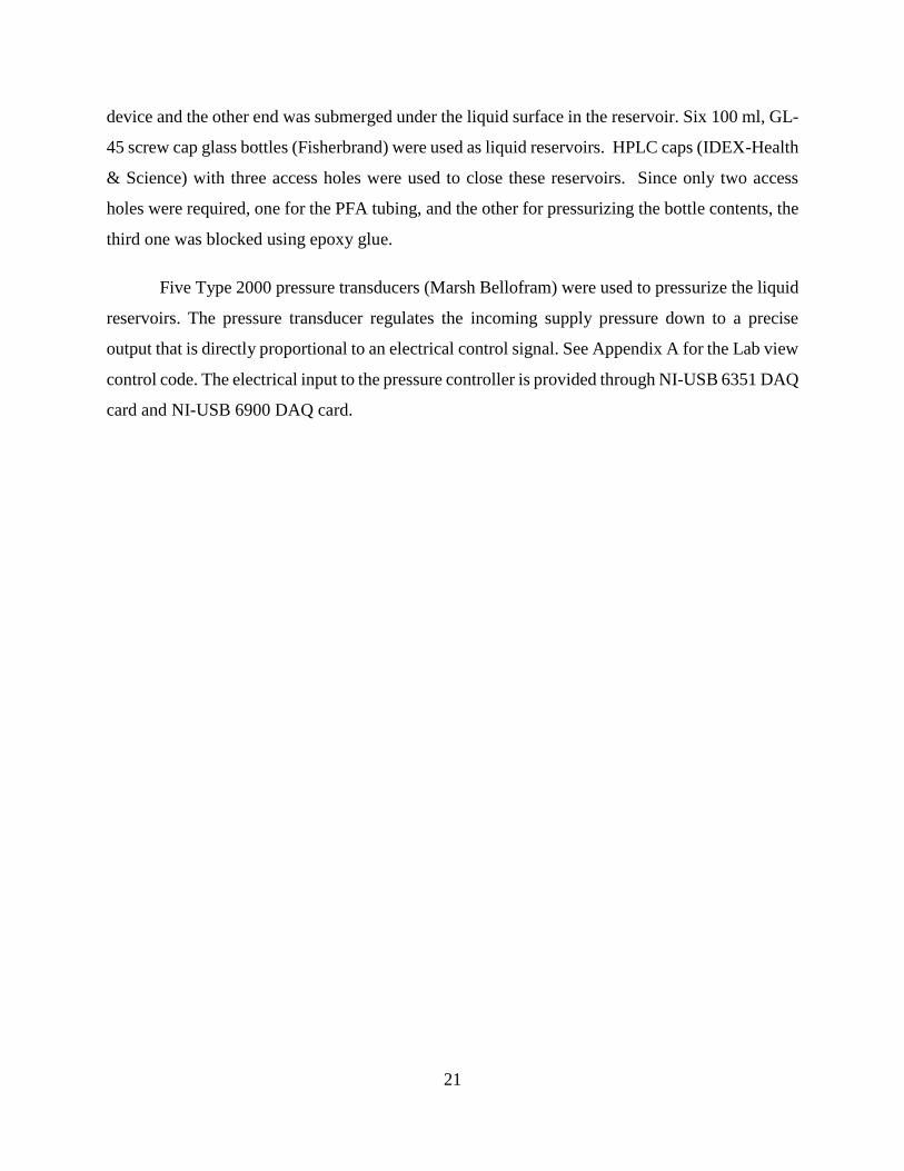
device and the other end was submerged under the liquid surface in the reservoir. Six 100 ml, GL-
45 screw cap glass bottles (Fisherbrand) were used as liquid reservoirs. HPLC caps (IDEX-Health
& Science) with three access holes were used to close these reservoirs. Since only two access
holes were required, one for the PFA tubing, and the other for pressurizing the bottle contents, the
third one was blocked using epoxy glue.
Five Type 2000 pressure transducers (Marsh Bellofram) were used to pressurize the liquid
reservoirs. The pressure transducer regulates the incoming supply pressure down to a precise
output that is directly proportional to an electrical control signal. See Appendix A for the Lab view
control code. The electrical input to the pressure controller is provided through NI-USB 6351 DAQ
card and NI-USB 6900 DAQ card.

22
Figure 3.8. Schematic of the experimental setup.
3.6 Materials and methods
As mentioned in Chapter 2, this work was performed for a model oil-water particle system
for which the interfacial properties are well characterized. The choice of fluid - fluid-particle
system was challenging because of multiple constraints of this system. The model system had to
be chosen such that:
1. The refractive index between the drop fluid and continuous fluid should be matched such
that the oil-water interface is very thin to enable better tracking of particle on the drop
surface.

23
2. The particles should be dispersed properly in both the continuous and dispersed phases,
but the particles should have greater affinity towards the dispersed phase than the
continuous phase.
3. The particles should have density similar to that of the fluids chosen to prevent settling in
the continuous phase and should be held inside the drop of the dispersed phase without
rupturing the drop.
4. The particles should not react or aggregate in either of the phases.
5. None of the two fluids chosen should be volatile in nature or swell the PDMS device.
With these restrictions, the following experimental system was used as the representative
system. Light mineral oil (Sigma Aldrich, 30cP) was used as the continuous phase. The refractive
index of mineral oil is 1.467 at 20 º C. Glycerol/water (70 v % glycerol) mixture was used as the
dispersed phase and its refractive index is 1.435 [53]. This glycerol/water composition was used
in order to almost match the refractive index [54] of the drop fluid with the suspending fluid. The
density and viscosity of 70 v % glycerol/water mixture were 1197.2 kg/m3 [55] and 35.5cP [56]
respectively. Hollow glass beads (Corpuscular Inc.) of density 1.01 g/cc and 10.0 µm mean
diameter were used as the particles in this study. The glass beads were suspended in light mineral
oil. Since the beads were hydrophilic in nature, after suspending the hollow glass beads in mineral
oil, the solution was sonicated for 3 minutes to suspend the beads well in the oil. During the course
of the experiments, the liquid reservoir containing the particles in solution was placed on a
magnetic stirrer and was stirred every half an hour to make sure that the glass beads do not
aggregate in mineral oil. All these fluids were used neat without adding any surfactants and were
used without further purification.
3.7 Centrifugation of Glass beads
Hollow glass beads of density 1.01 g/cc obtained from Corpuscular Inc. had mean diameter
of 11.5 µm with a standard deviation of ± 5. To further reduce the polydispersity, the hollow glass
beads were centrifuged [57] in a swinging bucket centrifuge (Cole Parmer) to obtain a mean
diameter of 10 µm for the glass beads with a standard deviation of ± 2.57. 300 mg of glass beads
was taken and 10 ml of DI water was added to it. A 50 ml plastic vial (Corning) was filled up to

24
40 ml and placed in the centrifuge. Another 50 ml plastic vial containing pure DI water was used
as a counter weight. The centrifuge was set to rotate at 500 rpm for 3 minutes. The suspension of
the glass beads in 10 ml DI water was added to the vial containing 40 ml DI water. Immediately,
the vial was closed and centrifuged. 15 ml of the centrifuged solution from the top was collected
using a 15 ml plastic syringe. Care had to be taken to not to disturb the suspension in the lower
layers. The withdrawn solution was expected to have glass beads a size range of 6-13 µm as
obtained from theoretical simulations. The suspension of 6-13 µm glass beads was further
centrifuged at 700 rpm for 9 minutes. 35 ml of DI water was taken in a 50 ml vial and was topped
with 15 ml of 6-13 µm glass beads. 20 ml of the centrifuged solution was withdrawn from the top
using a plastic syringe. As shown in Figure 3.9, the obtained solution had a mean diameter of 10.06
µm with a standard deviation of ± 2.57. This suspension was poured into a petri-dish and the beads
were dried in the oven for 9 h at a temperature of 75°C.
Figure 3.9. Size distribution of glass beads after centrifugation.

25
3.8 Circular Modification of the PDMS Channels
The drop when held at the constriction does not provide a perfect seal to the flow of the
fluid across it. The leakage of the fluid occurs because a drop cannot perfectly conform to the
rectangular cross-section of the PDMS channel. To overcome this problem, the rectangular cross-
section of the PDMS channel was converted to circular cross-section [58]. PDMS elastomer was
mixed with the pre-cursor in the ratio of 10:1 and degassed. The degassed PDMS elastomer was
taken in a 1 ml syringe fitted with an 18 gauge needle (BD Scientific). A small rigid PFA tubing
of 0.04 in. inner diameter was fitted on the tip of the needle to deliver the PDMS elastomer into
the device. The bonded PDMS device was preheated for 4 minutes at a temperature of 110°C. The
PDMS channel was taken off the hot plate and immediately the PDMS elastomer was introduced
into the device through the port having the constriction. When the PDMS was flushed out through
the other ports, the syringe was removed and nitrogen was delivered into the device using a PFA
tubing of .00625 in. inner diameter .Nitrogen was bubbled through the inlet having the constriction
at a pressure of 9 psi for around 15 minutes. Care had to be taken that nitrogen flowed out through
all the ports. With the tubing delivering the nitrogen into the device, it was again kept on the hot
plate at a temperature of 110°C. Once PDMS was cured in the device, the tubing delivering the
nitrogen was removed and the device was kept on the hotplate for an additional 20 minutes. The
schematic of the modification is shown in Figure 3.10.
26
Figure 3.10. Modification Procedure (Reproduced from [58]).
27
3.9 Method to confirm the close-to-circular cross-section of modified
PDMS Channel.
Confocal laser scanning microscopy (CLSM) was used to view the modified cross-section
of the rectangular PDMS channels. Aqueous solution of 0.01 mg/mL dextran molecules labeled
with fluorescein isothiocyanate (average molecular weight 70,000, a diameter of 6.0 nm [59] and
diffusion coefficient in water of 11 22.3*10 /m s ) [60] was injected into the microfluidic device.
A 200 μm depth scan was performed at increments of 10 μm in the direction perpendicular to the
imaging plane of the microfluidic device (z-direction). The wavelength of the laser used was 480
nm. The 3D reconstruction of the stacked CLSM image was used to show the rectangular cross-
section and the close-to-circular cross-section of the micro-channel. Figure 3.11 shows the
rectangular cross-section of the PDMS device before any modification. As seen in Figure 3.12, as
a result of modification, the channel corners are rounded, which prevents the leakage of particles
at the constriction.

28
Figure 3.11. Rectangular cross-section of the channel-at-large obtained by 3D reconstruction of
21 images.

29
Figure 3.12. Modified cross-section of the channel-at-large obtained by 3D reconstruction of
21 images.
3.10 Rendering the PDMS Channels Hydrophobic
The fabricated PDMS channels are inherently hydrophobic in nature [61].The plasma
bonding of the PDMS with its base rendered the PDMS channel hydrophilic in nature. The
hydrophobic nature of the bonded device had to be restored to make the PDMS surface oil-wetting.
The increase in contact angle between the drop phase and the PDMS channel was implemented by
coating the channel with hexamethyldisilazane (HMDS). The contact angles between drop phase
and PDMS before and after treatment is shown in Figure 3.13. The circularly modified PDMS
device was cleaned by sonicating in isopropyl alcohol for 2 minutes and subsequently dried with
nitrogen. The device was then kept on a hot plate at 86°C. HMDS was filled in a 20 ml glass vial
fitted with a rubber cork. Four needles of 22 gauge diameter were fixed into a PFA tubing of 0.04
in. diameter using Parafilm. One end of the needle was introduced through the rubber cork into the
vial and the other end containing the tubing was introduced into the device. All but one of the ports
30
was left open to the atmosphere. A long steel needle was introduced into the vial which delivered
the nitrogen into the vial. The nitrogen helped to bubble HMDS into the channel and the constant
heat helped in the deposition of HDMS vapors in the channel, rendering it hydrophobic. Nitrogen
was bubbled into HDMS for 3 h.
Figure 3.13. Contact angles of drop phase on cured PDMS. a) Contact angle of 45on cured
PDMS after oxygen plasma etching, b) Contact angle of 65.0on cured PDMS, c) Contact angle
of 101.4on cured PDMS after treatment with HMDS.
3.11 Contact Angle measurement
Sigma Force Tensiometer - Model 700 was used to measure the interfacial tension 1 2L L
which was found to be30.8 mN/m . Rame-Hart Goniometer - Model 100-00-115 was used to
determine the contact angle, , which was found to be 37.1 . For carrying out experiments to study
the effect of viscosity ratio on particle capture efficiency, the contact angles of various systems of
drop phases were measured which were shown in Figure 3.14.

31
Figure 3.14. Contact angles in mineral oil. a) DI water on glass 25.4 , b) Glycerol/DI water
mixture on glass 35.1 , c) Glycerol/IPA mixture on glass 65.4 .
3.12 Experimental Procedure
The water-in-oil droplet was generated using a T-junction on the inlet (I1). The
glycerol/water mixture and the oil was maintained at a pressure differential such that the flow rate
of the suspending phase was sufficient enough to create short slugs of the dispersed phase. At these
low flow rates, interfacial forces dominates the hydrodynamic stresses [62], and hence, the droplet
completely spans the channel width. In this regime, the size of the water slug is given by the
following relationship:
1 .s water oilL w Q Q (3.3)
Here, sL is the length of the slug, w is the channel width, waterQ and oilQ , are the flow rates
of water and oil, respectively, and is a constant which depends on the geometry of the T-junction
[62]. These short slugs spanned the channel depth and thus no gravity effects are observed. When
a few droplets were formed at the junction, the water was cut off and the last slug traversed through
the channel and the water drop is held firmly at the constriction by applying suction at the other
inlet 2I . The inlet 2I with the constriction served as the suction arm. The constriction served as a
region of high shear stress with respect to the rest of the device and helped to break the desired

32
sized drop from the slug. As shown in section 3.3 in Figure 3.5, the inlet 2I with the constriction
and the negative pressure applied on it acts like a micropipette aspiration device. The rest of the
slugs left the device through exits 1O or 2O . The pressure transducer connected to inlet 1I had two
liquid reservoirs connected to it. One reservoir contained the particles suspended in mineral oil
and the other reservoir had neat mineral oil in it and flow through the reservoirs was controlled by
a one way valve (IDEX-Health & Science). One valve was inserted in the flow line and the other
valve was installed in the pressure line. This arrangement allowed alternating the pressurization of
either of the liquid reservoirs and, in turn the flow through them when required. Once the
water/glycerol drop was held at the constriction, the reservoir containing the particles was
pressurized and the particles were made to impinge the drop. The time taken for the particles to
settle in the channel sett , is calculated using Stokes law of settling:
22
9
set
p p oil
Bt
R g
(3.4)
where (device depth)is100 μmB , is 1.05 g/cc, is 0.85 g/cc , R is 5 μm and is 30 cP p oil p .
The settling time is 210 s, which is much higher than the residence time or interaction time of
the particles. This states that the settling of particles in the microfluidic aspiration device is
unimportant.
3.13 Distribution of incoming particles along the channel width
Figure 3.15 shows the fraction of particles entering the device along the width ' 'y at 0z
when the velocity was 0.718 mm/s. From the figure, it can be said that particles were equally
distributed along the width of the channel without any bias towards any particular streamline.

33
Figure 3.15. Fraction of particles entering the channel along 100y m at z = 0 at a velocity
of 0.718 mm/s.
3.14 Analysis Procedure
The particle-drop impingement process was recorded by a 16-bit monochrome camera
(Retiga 2000R, Q-imaging) using Nikon’s NIS Software. Then NIS Viewer version 4.3 was used
to extract all the frames from the recorded video. Using the Image Analysis and Image Processing
toolbox in MATLAB 2012a, the obtained frames are read and an intensity adjustment was done
on the frames using the command imcontrast. Different image analysis and enhancement tools
available in Image Processing toolbox in MATLAB were used to analyze the images. Once the
image enhancement was done, image subtraction between successive frames used to locate the
movement of the particle over multiple frames. In each frame, every particle was located using
Hough transform and the corresponding centroids and particle radii were saved. To correlate the
position of a particle between successive frames and identify its trajectory, several criteria were

34
used: distance between the particle centroids in successive frames, changes in slope of trajectory,
and velocity variation along a trajectory. Along with the matched centroids, the particle radius was
also saved. During the identification process, the water drop was masked to prevent any counting
of the particles which were already captured by the water drop. Once the particles were identified,
the drop was de-masked and the fate of each particle was decided based on its ultimate location. During the identification process, the velocity and location with respect to the center of the device,
of the each of the particles entering the channel was tracked. The block diagram of the particle
tracking algorithm is shown in Figure 3.16.
Figure 3.16. Block diagram of multiple particle - tracking algorithm.

35
Chapter 4 Experimental Results and Discussion
In our study, the average efficiency, , of capture of a particle by a water droplet is defined as
,
2
d
d
y dy
d
(4.1)
where y is the local efficiency of capture of particles along a streamline beginning at the
ordinate y, and d is the limiting ordinate beyond which particle capture would not occur. The total
spatial spread of the distribution, -d to d, was fairly constant for the experiments, with a value of
about 30 m. The function y was determined by placing particles arriving at the drop into
finite-sized bins in y. The bin size was chosen such that there were between 75 to 100 particles,
which places the error due to the Poisson statistics of particle counting at about 10% in each bin.
Figure 4.1 shows the variation of y within the limiting ordinates. Experiments were conducted
to study the effect of parameters such as velocity, drop size and nature of capturing medium on the
particle - capture efficiency. The effect of each parameter is discussed in section 4.1 below. In
section 4.2, we will discuss the possible mechanisms influencing the trends of capture efficiency
for each parameter.

36
Figure 4.1.Variation of y within the limiting ordinates.
4.1 Experimental Results
4.1.1 Effect of particle velocity on capture efficiency
The local efficiency of capture, ( )y , is shown in Figure 4.2 for different velocities, when
the drop size was maintained at 99.7 2.3 μm with = 1 . ( )y usually achieved a maximum
near the centerline y = 0, and reduced in magnitude as we moved away from the centerline. Figure
4.3 shows the average particle capture efficiency, , as a function of the particle velocity.
increased with particle velocity, with a maximum efficiency of 36 % at a velocity of 1 mm/s . The
error bars for each of the data points represents the variance in capture efficiency obtained by
analysing the data over multiple time intervals. Figure 4.4 shows the variation in capture efficiency
with time for a velocity of 1 mm/s for a drop diameter of 100 μm with = 1 . This experiment
recorded at 23.84 fps comprised 40000 frames which were split equally into four parts each having
10000 frames and the variation in capture efficiencies for each of the groups is plotted against the

37
total time elapsed. The local efficiency of capture, ( )y , is shown in Figure 4.5 for different time
intervals for a velocity of 1 mm/s for a drop diameter of 100 μm with = 1 .
(a) (b)
(c) (d)
38
Figure 4.2. Plots of particle-capture efficiency against velocity for a drop of diameter
99.7 2.3 μm with =1 . (a) Velocity of 0.666 mm/s, (b) Velocity of 0.691 mm/s, (c)
Velocity of 0.718 mm/s, (d) Velocity of 1.009 mm/s and (e) Velocity of 1.52 mm/s.
(e)

39
Figure 4.3. Plot of capture efficiency against applied velocity for a drop of diameter
99.7 2.3 μm with =1 at mid-plane (z = 0) and y between ± 10 µm from device center (y
= 0).

40
Figure 4.4. Plot of capture efficiency against the total time elapsed for a velocity of 1 mm/s for
a drop diameter of 100 μm with = 1 .

41
Figure 4.5. Plot of capture efficiency against y for different time intervals for a velocity of 1 mm/s,
drop diameter of 100 µm with λ=1. (a) Time = 7 mins, (b) Time = 14 mins (next 7 mins of the
experiment), (c) Time = 21 mins (next 7 mins of the experiment) and (d) Time = 28 mins (next 7
mins of the experiment).
(a) (b)
(c) (d)

42
4.1.2 Effect of drop size on capture efficiency
The local efficiency of capture, y , shown in Figure 4.6 for different drop sizes for an
average velocity of 1.52 mm/s and 1 , exhibits the expected trend: maximum near the
centerline y = 0, and decaying away from the centerline. Figure 4.7 shows the average particle
capture efficiency, , as a function of the drop diameter. With increase in drop diameter,
increased. The maximum efficiency of 28 % was observed for a drop size of 100 µm.
(a) (b)
(c) (d)

43
Figure 4.6. Plots of capture efficiency against drop size for a velocity of 1.52 mm/s and 1 .
(a) Drop of 52 µm, (b) Drop of 79.5 µm, (c) Drop of 84.1 µm and (d) Drop of 100 µm.
Figure 4.7. Plot of capture efficiency against drop diameter for a velocity of 1.52 mm/s and
1 at mid-plane (z = 0) and y between ± 10 µm from device center (y = 0).
4.1.3 Effect of nature of capturing medium on capture efficiency
The experimental matrix shown in Table 4.1 was designed to understand the effect of
nature of capturing medium on particle capture efficiency. This table also details the average
particle capture efficiency, . The local efficiency of capture, y , is shown in Figure 4.8 for
different capturing mediums, when the average velocity was maintained at 0.718 mm/s at a drop
size of 100 µm. For DI water as drop phase, was low at 15 % and increased to 32 % when
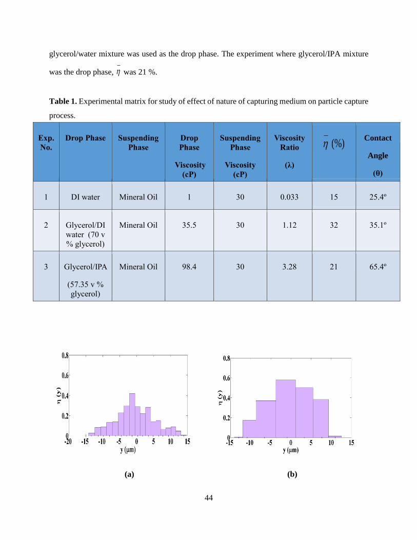
44
glycerol/water mixture was used as the drop phase. The experiment where glycerol/IPA mixture
was the drop phase, was 21 %.
Table 1. Experimental matrix for study of effect of nature of capturing medium on particle capture
process.
Exp.
No.
Drop Phase Suspending
Phase
Drop
Phase
Viscosity
(cP)
Suspending
Phase
Viscosity
(cP)
Viscosity
Ratio
(λ)
(%) Contact
Angle
(θ)
1 DI water Mineral Oil 1 30 0.033 15 25.4º
2 Glycerol/DI
water (70 v
% glycerol)
Mineral Oil 35.5 30 1.12 32 35.1º
3 Glycerol/IPA
(57.35 v %
glycerol)
Mineral Oil 98.4 30 3.28 21 65.4º
(a) (b)
45
Figure 4.8. Plots of capture efficiency against nature of capturing medium. (a) DI water as drop
phase, (b) Glycerol/water mixture as drop phase and (c) Glycerol/IPA mixture as drop phase.
4.2 Discussion
Whether or not a particle is captured by the drop depends on the interaction time, It , of the
particle with the drop, relative to the characteristic time, Ct , required for particle capture. The
interaction time is the time spent by the particle “colliding” (defined more carefully later) with the
drop-suspending fluid interface. The characteristic time of capture can be viewed as the time
required for the particle to reach the interface and break/penetrate it, if the “collision” time with
the drop is indefinitely long.
If C It t , the particle will be captured; if C It t , the particle will escape without capture.
In this following sub-sections, we first explain in detail the interaction process of the
particle with the drop. We will then comment on the mechanisms that can affect the capture
process, and on the variables influencing the capture time, Ct , for each mechanism. Finally, we
(c)

46
will compare these trends with our experimental results of the capture efficiency, and identify the
dominant mechanism for particle capture.
4.2.1 Interaction time It
Since the interaction time is influenced by hydrodynamics, a detailed simulation of the
motion of the particles in the flow field of our geometry is required. This appears to be a
complicated calculation, but is simplified considerably by two facts. First, the Reynolds number,
which quantifies the effect of inertial forces to viscous forces in a flow field, is small, so that flow
is laminar. Second, the Stokes number, which measures the ability of a particle to deviate from a
fluid streamline due to inertia, is small 610Stk , as explained in Appendix B. With these
simplifications, the particles can be assumed to essentially follow the streamlines. The simulation
of the flow field in the experimental geometry was performed in COMSOL 4.3b. The details of
the implementation of these simulations are discussed in Appendix B.
The center of mass of the particle can approach the interface only as close as the particle
radius. Since the mean particle diameter in our experiments was about 10 µm, streamlines within
a boundary of 5 µm from the surface of the drop were considered for interaction time computations.
Figure 4.9 shows a drop and the boundary along with streamlines within this region.
47
Figure 4.9. Streamlines at mid-plane ( 0)z of the microfluidic aspiration device.
The interaction time It was defined as the time spent by particles, due to flow, in the region
where particles first enter the bounding region (point A in Figure 4.10), up to the point where the
particles exit the bounding region (point B in Figure 4.10). The “collision” between the particle
and the interface is said to occur between these two points, and the time elapsed between the entry
and exit points is the interaction time It . In order to evaluate It , COMSOL’s LiveLink feature
with MATLAB was employed. The variation of It with y for different values of the z co-ordinate
is shown in Figure 4.11. At z-planes closer to the walls, the interaction time is high owing to lower
velocities there. At the mid-plane, the velocity is maximum, leading to the least interaction time
with the drop surface. Typical interaction times are of the order of 0.01 seconds or higher.

48
Figure 4.10. Streamline within the bounding region. The region between point A and C is the
approach phase and the region between point C and B is the separation phase.

49
Figure 4.11. Plot of total interaction time of particle within the bounding region along
100y m the device width for different Z-planes z = ± 50 μm .
Note that the lower limit of y co-ordinates shown in Figure 4.11 is not zero. This is because,
the interaction time diverges as y approaches zero. As may be seen in Figure 3.16, the velocity at
the drop surface for y = 0 is identically zero. This point is known as the stagnation point, and any
particle travelling along the streamline at y = 0 will spend an infinite time interacting with the drop
in this head-on collision. Of course, due to continuity, the stagnation point is also a saddle point,
and slight perturbations from the y = 0 ordinate will lead to finite, albeit long, interaction times.
Thus, particles in the vicinity of the y = 0 streamline decelerate as the interface is approached,
allowing large interaction times with the drop surface, and thus leading to a high probability of
particle capture. As we move further away from the y = 0 streamline, the particles attain higher
velocities and spend increasing smaller times interacting with the interface, and should experience
lower capture efficiencies. For particles approaching along the bounding streamline, the
interaction time, and hence, the capture efficiency, are zero. This explains the bell-shaped nature
of the capture efficiency histograms in Figures 4.2, 4.6 and 4.8.

50
We digress here briefly to discuss an element of the particle interface collision that will be
useful for subsequent discussions. The collision of the particle with the interface can be divided
into two phases: an approach phase, in which hydrodynamic forces push the particle towards the
interface (point A to point C in Figure 4.10), and a separation phase, in which the hyrdoynamic
force is reversed and the particle is pulled away from the interface (point C to point B in Figure
4.10). The characteristic scales of the compressive force in the approach phase and the extensional
force in the separation phase are, both, given by 2
pGR , where is the viscosity of the suspending
fluid, and G is the characteristic strain rate of the flow. We will employ this scale subsequently to
estimate drainage times and detachment probabilities.
4.2.1 Particle-capture process
Having discussed the interaction time, we will now analyze the various steps involved in
the capture process to determine the rate determining step that influences the capture efficiency.
We remind the reader of these steps:
1. Hydrodynamic film drainage
2. Instability of the film
3. Bridge Formation / attachment
4. Motion of Contact Line
5. Engulfment
First, we explore the importance of hydrodynamic film drainage on particle capture [63]
[64] [65] [66] [67] [68] [Step 1, see Figure 2.2(a)]. A scaling analysis (detailed in Appendix C.1)
was implemented to determine the film drainage time Dt between a rigid particle of radius pR and
a drop of radius R . The drop is held stationary and the particle approaches the drop with a
compressional force 2~ pF GR as shown in Figure 4.12, which is balanced by the lubrication
forces arising from the drainage of the thin film.
51
Figure 4.12. Schematic of a particle of radius pR being pushed against a water drop of radius
R by a force F . In this schematic, the particle and the drop are separated by a thin film of
height h . The pressure in the thin film scales as the Laplace pressurepR .
Assuming the azimuthal extent of the contact of the film with the particle to be constant, the scaling
analysis yields the hydrodynamic drainage time as
3 2
,2
p
D
c
Ca Rt
Gh
(4.2)
where, Ca is Capillary number defined as:
1 2
.p
L L
GRCa
(4.3)
52
is the viscosity of suspending phase, pR is the radius of particle, G is the strain rate, ch is the
critical film thickness and 1 2L L is the interfacial tension.
Values of strain rates of 50 - 80 s-1, yield capillary numbers ranging from - 42.5 10 to
- 44 10 . For critical film thicknesses varying from 1 to 10 nm, the drainage time, Dt , is extremely
short: - 5O (10 ) to
- 6O (10 ) . If film drainage were the rate determining step, since
3 2
~ 1,2
pD
I c
Ca Rt
t h
nearly all particles travelling within the bounding streamline region would
enter the drop, achieving 100% particle-capture efficiency. This, however, is not seen in
experiments. The characteristic time scale for instability of the film instt [Figure 2.1(b)] initiated
by long range attractive forces between the particle and the drop after achievement of the critical
film thickness, is shorter than the time scale for hydrodynamic film drainage, due to the additional
attractive force pulling the particle towards the interface. Also, when the applied strain rate is
increased, D It t increases, so the capture efficiency should decrease. However, we observe the
opposite trend in our experiments. Therefore, it can be concluded that in our study, hydrodynamic
film drainage and the instability of the film are not the rate-limiting steps for particle capture, and
do not affect the dynamics of particle-capture process.
Before elaborating on the role of bridge formation and attachment in particle-capture, it is
useful to first consider the forces required to detach a particle lodged at the interface. The force
( )pullF required to pull the particle off the interface (see Figure 4.13) is given by:
2~ .pull pF GR (4.4)

53
Figure 4.13. Forces acting on a particle attached to the interface along with the motion
of the contact line.
The contact-line pinning force ( )CLF acting along the interface is given by
1 2
~ ,CL L LF l (4.5)
where, l is the length of contact line. If the particle is to be detached from the interface, the
condition
1 2
2
1, or ,p
c
L L
GRl l
l
(4.6)
should be satisfied, where the critical contact line length for detachment, lc, is
1 2
2
Ca p
c p
L L
GRl R
(4.7)

54
Since our characteristic capillary numbers are small, 4O (10 )
, for 10 m particles, the
critical contact line length for detachment is of the order of the magnitude of a nanometer. This
suggests that once even an extremely small region of the drop contacts the particle, the
characteristic hydrodynamic forces in our experiments that pull the particle are not adequate to
detach the particle off the interface. Therefore, any dynamics of the capture process and related
capture efficiencies must arise from the step in between steps 1 & 2 and step 4: bridge formation.
We will now explore the possibility of the intermediate step, bridge formation, by
extending the hole nucleation theory for emulsion droplets [44] [45] [46] [47]. We assume that
after the film drainage and instability steps, the particle comes to a separation, h, from the drop,
beyond which the formation of a drop fluid bridge is required to create a contact line. However, as
shown in Appendix C.2, the formation of the bridge requires a finite amount of energy depending
on its film thickness and the bridge radius. The critical bridge radius,C
r , beyond which the bridge
continues to grow in radius spontaneously is given by
1 cosC
hr
(4.8)
where is the contact angle defined with respect to the drop phase. As 0 , the particles can
be perfectly wetted by the drop fluid and the bridge radius is simply half the film thickness. As
, the bridge radius becomes infinite, due to the non-wetting nature of the drop fluid with
respect to the particle phase. The energy required for transition from state 1 to state 2 in Figure
4.14 is
1 2
2
.1 cos
L L hE
(4.9)
55
Figure 4.14. Schematic for the bridge-formation theory.
For the glycerol/DI water solution – mineral oil experiments, the interfacial tension 1 2L L
was found to be 30.8 mN/m, and the contact angle was 37.1º, The energy change relative to the
thermal energy, Bk T , at room temperature (25ºC) for this system is
216.9 ,B
Eh
k T
(4.10)
where h is in nm. Since the bridge formation is driven by thermal fluctuations over the above
activation energy barrier, the time taken for bridge formation Bt should be
0 exp .B
B
Et t
k T
(4.11)
56
The prefactor 0t is expected to depend on two time scales. One being the thermodynamic
time scale for the frequency of film fluctuations t 1 kf B T . The other time scale is expected to
scale as the capillary time scale 1 2
~v L Lt h based on the fluid with the higher viscosity, as the
formation of the bridge occurs by motion of the drop fluid over the length scale h. However, more
systematic experiments have to be conducted for the confirmation of this model.
Thus, the scaling for the bridge formation time is
1 2
2
0~ t exp ,1 cos
L L
B
B
ht
k T
(4.12)
It is the bridge formation time relative to the interaction time that will determine the efficiency of
capture.
1 2
2
0~ Gt exp ,1 cos
L LB
I B
ht
t k T
(4.13)
Here we have taken the interaction time to scale as G-1. The smaller the ratio /B It t , the
greater the probability of capture. We see that this ratio is extremely sensitive to the film thickness.
Any factor that influences the film thickness, e.g. hydrodynamic forces pushing the particle, will
affect the bridge formation time, and hence the probability of capture, strongly.
Substituting the numbers for the glycerol solution – mineral oil experiments, we get, for a
characteristic strain of 10 s-1,
2
0~ 10 t exp 16.9B
I
th
t (4.14)
where the film thickness is in nm. From Eq. (4.14) it is evident that h needs to be of the order of
a nanometer to yield bridge formation times that are of the order of the interaction time. The
theoretical capture efficiency of particles was calculated by [69] [70]:
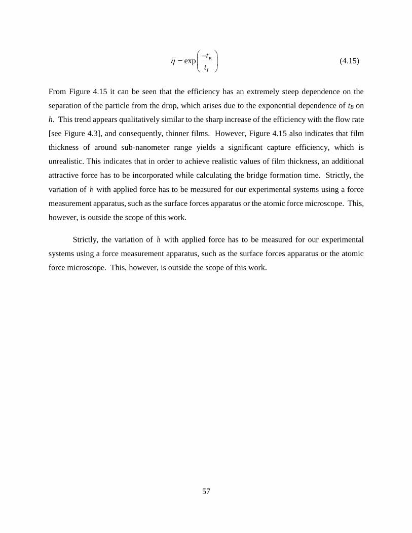
57
exp B
I
t
t
(4.15)
From Figure 4.15 it can be seen that the efficiency has an extremely steep dependence on the
separation of the particle from the drop, which arises due to the exponential dependence of tB on
h. This trend appears qualitatively similar to the sharp increase of the efficiency with the flow rate
[see Figure 4.3], and consequently, thinner films. However, Figure 4.15 also indicates that film
thickness of around sub-nanometer range yields a significant capture efficiency, which is
unrealistic. This indicates that in order to achieve realistic values of film thickness, an additional
attractive force has to be incorporated while calculating the bridge formation time. Strictly, the
variation of h with applied force has to be measured for our experimental systems using a force
measurement apparatus, such as the surface forces apparatus or the atomic force microscope. This,
however, is outside the scope of this work.
Strictly, the variation of h with applied force has to be measured for our experimental
systems using a force measurement apparatus, such as the surface forces apparatus or the atomic
force microscope. This, however, is outside the scope of this work.
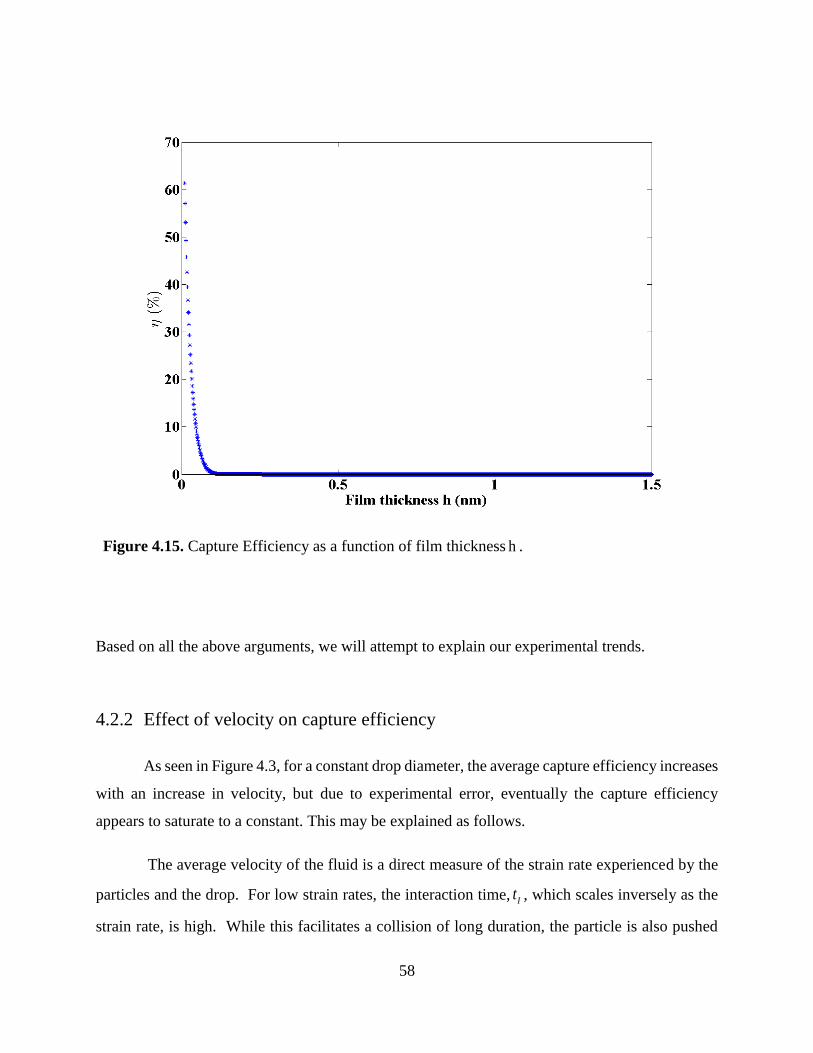
58
Figure 4.15. Capture Efficiency as a function of film thickness h .
Based on all the above arguments, we will attempt to explain our experimental trends.
4.2.2 Effect of velocity on capture efficiency
As seen in Figure 4.3, for a constant drop diameter, the average capture efficiency increases
with an increase in velocity, but due to experimental error, eventually the capture efficiency
appears to saturate to a constant. This may be explained as follows.
The average velocity of the fluid is a direct measure of the strain rate experienced by the
particles and the drop. For low strain rates, the interaction time, It , which scales inversely as the
strain rate, is high. While this facilitates a collision of long duration, the particle is also pushed

59
weakly towards the interface, and the film thickness between the particle and the interface is high.
Therefore, the probability of bridge formation and particle capture are low, hence the low capture
efficiency. As the strain rates are increased, the interaction time decreases, but the compressive
force exerted on the particle increases, thereby decreasing the film thickness and improving the
probability of bridge formation. This leads to an increase in capture efficiency with an increase in
the strain rate. For very high strain rates, while the film thickness is further reduced, the interaction
time available for the probabilistic event of bridge formation decreases, thus reducing the capture
efficiency. This suggests that there is an optimal velocity for maximum particle capture.
4.2.3 Effect of drop size on capture efficiency
As seen in Figure 4.7, the capture efficiency increases with drop size for fixed velocity and
viscosity ratio. This can be explained as follows. As the drop size increases for a fixed incoming
flow velocity, the strain rate of the flow, which scales as the velocity relative to the drop size,
decreases. A reduced strain rate, provides a longer interaction time of the particles with the drop.
Hence, a greater capture efficiency is observed for the larger drops. Now, it may be argued that
a reduced strain rate could also decrease the capture efficiency due to higher film thickness and a
lower probability of bridge formation, as was mentioned in section 4.2.2 for the varying velocity
experiments. However, the strain rates for the varying diameter experiments were greater than or
equal to the highest strain rates in the varying velocity experiments, as can be seen in Figure 4.16.
This suggests that the compressive forces required to bring the particle closer to the interface were
sufficient to lead to a high probability of bridge formation and capture.
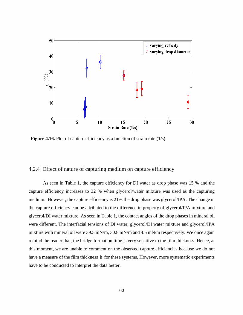
60
Figure 4.16. Plot of capture efficiency as a function of strain rate (1/s).
4.2.4 Effect of nature of capturing medium on capture efficiency
As seen in Table 1, the capture efficiency for DI water as drop phase was 15 % and the
capture efficiency increases to 32 % when glycerol/water mixture was used as the capturing
medium. However, the capture efficiency is 21% the drop phase was glycerol/IPA. The change in
the capture efficiency can be attributed to the difference in property of glycerol/IPA mixture and
glycerol/DI water mixture. As seen in Table 1, the contact angles of the drop phases in mineral oil
were different. The interfacial tensions of DI water, glycerol/DI water mixture and glycerol/IPA
mixture with mineral oil were 39.5 mN/m, 30.8 mN/m and 4.5 mN/m respectively. We once again
remind the reader that, the bridge formation time is very sensitive to the film thickness. Hence, at
this moment, we are unable to comment on the observed capture efficiencies because we do not
have a measure of the film thickness h for these systems. However, more systematic experiments
have to be conducted to interpret the data better.
61
Chapter 5 Conclusions and Future Work
5.1 Conclusions
In this work, we have discussed the development of a microfluidic aspiration device which
can be used to study particle-drop collision experiments. The experimental results were validated
by demonstrating a favorable agreement with simulations. We have established the fact that at low
capillary numbers 410O , the bridge formation step and not hydrodynamic film drainage was the
rate limiting step for particle capture. For our experimental regime, it was observed that capture
efficiency increased with an increase in flow rate and collector drop radius. It was found that at a
strain rate of 110 s (see Figure 4.16), a drop of 100 µm had a maximum capture efficiency of
around 36 %. The drop is also not expected to break up under these conditions, as the
corresponding capillary number is on the order of 0.01, which is less than the critical capillary
number for drop fracture [71] [72] .
There has been intense research in the area of colloid filtration in a porous medium, where
colloidal particles introduced via flow into the medium interact with the medium surfaces, and are
trapped [73] [74] [75] [76]. The porous medium is typically comprised of larger spherical
particles, whose ability to collect the smaller colloids is a complicated function of hydrodynamics
and particle-colloid interaction forces. The capture efficiency of a collector particle, o , is the
ratio of the number of colloids captured by the collector to the total number of colloids intercepted
by the projected area of the collector particle [74]. This situation is analogous to the case
considered in this work, except that the interface of the collector particle is deformable, and that
the nature of the interaction forces is different. The capture efficiencies reported by us can be
easily interpreted in the colloid filtration context if our average efficiencies are multiplied by the
geometric factor d
R, i.e.
o
d
R .
The observed trends were obtained for laminar flow conditions where viscous forces are
dominant and the particle-drop interaction time is given by the inverse of the applied strain rate.
However, in order to implement these results to design a mixer under industrial conditions, a
turbulent flow regime must be considered. In turbulent flows, the Kolmogorov scale defines the

62
transition between two regimes [77] [78] namely the turbulent viscous regime and the turbulent
inertial regime. The Kolmogorov length scale and time scale, , are defined as [35]:
1 43
(5.1)
and
1 2
(5.2)
where, is the momentum diffusivity of the fluid and is the mean energy dissipation rate per
unit mass of continuous phase. For length scales smaller than the Kolmogorov length scales,
viscous forces are dominant and the collision dynamics and the characteristic strain rates of
interaction are on the order of the inverse of . Therefore, if the particles and drops are smaller
than the Kolmogorov length scale, the inverse of the Kolmogorov time scale must be equal to the
optimum strain rate identified in this work to ensure highest capture efficiencies.
This restriction specifies the maximum drop size that should be expected in the inertial
sub-regime of the turbulent flow. The characteristic time scale in this regime is given by
1/3
2 / ,D and the mixer should be designed to have this time scale as the inverse of the
optimum strain rate for efficient particle capture.
The results of this work are not restricted only to the oil sands industry, but as mentioned
in Chapter 2, find application in industries such as oil extraction from oil seeds using hexane and
in air pollution control where water drops serve as collectors for removal of aerosols. It also finds
application in the isolation of desired biological components from cell mixtures [19] and in the
oxy-fuel combustion technology for NO2 removal from flue gases which are released during coal-
fired power generation [20].
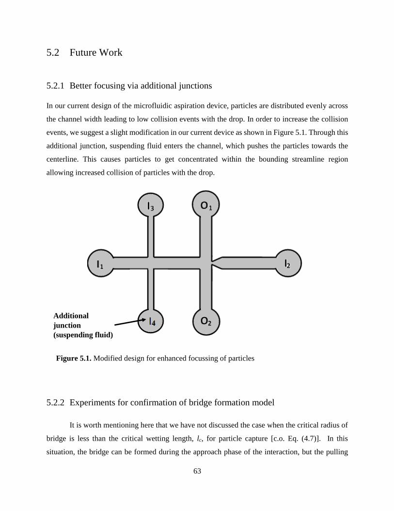
63
5.2 Future Work
5.2.1 Better focusing via additional junctions
In our current design of the microfluidic aspiration device, particles are distributed evenly across
the channel width leading to low collision events with the drop. In order to increase the collision
events, we suggest a slight modification in our current device as shown in Figure 5.1. Through this
additional junction, suspending fluid enters the channel, which pushes the particles towards the
centerline. This causes particles to get concentrated within the bounding streamline region
allowing increased collision of particles with the drop.
5.2.2 Experiments for confirmation of bridge formation model
It is worth mentioning here that we have not discussed the case when the critical radius of
bridge is less than the critical wetting length, lc, for particle capture [c.o. Eq. (4.7)]. In this
situation, the bridge can be formed during the approach phase of the interaction, but the pulling
Additional
junction
(suspending fluid)
Figure 5.1. Modified design for enhanced focussing of particles

64
hydrodynamic force in the separation phase is sufficient to unwet the particle and detach it from
the interface. This also requires that the contact line does not move fast enough to exceed the
critical wetting length during the approach phase. This is supported by recent holographic
measurements of particle motion that indicate the contact line motion times are on the order of
hours [79] , which is much greater than our interaction times of the order of 0.01 seconds. We are
currently undecided about the possibility rc < lc in our experiments. The length scale, lc, is of the
order of a nanometer, but with the addition of the attractive force in the bridge formation time, we
expect critical bridge radius greater than lc. On the other hand, the explanation based on the bridge
formation time predicts a sharp rise in the efficiency of capture beyond a critical flow rate [see
Figure 4.3]. It is not immediately obvious what the variation of the efficiency with strain rate
should be for the rc < lc regime. This investigation is left to future work.
5.2.3 Alternative design for the microfluidic aspiration device
The microfluidic aspiration device used in our study required the modification of
rectangular cross-section of the device into circular by the method developed by Lindsey et al.
[58]. However, this method involves great level of expertise in fabricating good circular channels.
During the process of modification, many PDMS devices had to be sacrificed. The drop particle
collision-capture experiments can be conducted in an alternative geometry. A silica capillary of a
finer bore was introduced into the arm containing the constriction and epoxy was used to stick the
capillary firmly to PDMS device and to prevent leakage. Water was introduced into the channel
through the capillary and a drop was held at the tip of the capillary by applying a strong negative
pressure as depicted in Figure 5.2. This design also eliminates the necessity of a T-junction to
introduce water drops into the channel.

65
Figure 5.2. Drop held at the tip of a silica capillary in the microfluidic aspiration device
(Image taken from Rohit Sonthalia).
5.2.4 Coalescence of two soft particles
The microfluidic aspiration device can be used to carry out controlled head-on collisions
between two soft particles at definite strain rate by holding one the particles stationary at the
constriction and pushing the other particle with a constant force F̂ towards it. Head-on collisions
can be carried out between both equal and unequal sized drops in this device, as shown in Figure
5.3 for two unequal sized water drops.

66
Figure 5.3. Drop Coalescence in the microfluidic aspiration device (Image taken from Rohit
Sonthalia).
5.2.5 Compatibility with the material of construction
In our work, glycerol/water drop was used to capture the glass beads suspended in mineral
oil in a PDMS-based microfluidic aspiration device. The motivation behind this work was to
develop a microfluidic aspiration device to capture clay particles suspended in bitumen by process
water used in the oil sands industry. However, due to the compatibility issues of PDMS with
toluene and other liquids [80], our PDMS-based device cannot be used to carry out studies using
bitumen.
But having established a standard procedure for carrying out particle-drop collision experiments,
a glass based microfluidic aspiration device as shown in Figure 5.4 can be fabricated for trapping
clay particles in bitumen by a water drop. In addition to the unreactive nature of glass with toluene,
the device can be rendered hydrophobic or hydrophilic more easily when compared to PDMS.

67
Figure 5.4. Glass-based microfluidic aspiration device (Image taken from Rohit Sonthalia).

68
References
[1] E. D. Attanasi and R. F. Meyer, "Natural Bitumen and Extra-Heavy Oil," Survey of Energy
Resources, vol. 22, pp. 123-140.
[2] "Alberta's Oil Sands :Opportunity,Balance," 2008.
[3] "Sustainable Development Business Case Report, Clean Conventional Fuel-Oil and Gas
version 1, 2006 Nov 1," 2006.
[4] [Online]. Available: http://www.capp.ca/ canadaIndustry/ oilSands/ Energy-Economy/
Pages/ default.aspx#sUbptoilP04R.
[5] A. Hooshiar, P. Uhlik, Q. Liu, T. H. Etsell and D. G. Ivey, "Clay minerals in nonaqueous
extraction of bitumen from Alberta oil sands Part 2. Characterization of clay minerals," Fuel
Processing Technology, vol. 96, pp. 183-194, 2012.
[6] R. Butler, Thermal Recovery of Oil and Bitumen, Prentice-Hall, 1991, p. 104.
[7] "VAPEX and Solvent Technology".
[8] "The THAI Process," Petrobank Energy and Resources Ltd., 2008.
[9] J. Alvarez and H. Sungyun, "Current Overview of Cyclic Steam Injection Process," Journal
of Petroleum Science Research. Science and Engineering , 2013.
[10] A. Hooshiar, P. Uhlik, Q. Liu, T. H. Etsell and D. G. Ivey, "Clay minerals in nonaqueous
extraction of bitumen from Alberta oil sands Part 1. Nonaqueous extraction procedure," Fuel
Processing Technology, vol. 94, no. 1, pp. 80-85, 2012.
[11] M. Gray, Z. Xu and J. Masliyah, "Physics in the oil sands of Alberta.," Physics Today, vol.
62, p. 31, 2009.
[12] D. Woynillowicz, C. S. Baker and M. Raynolds, "Oil Sands Fever-The Environmental
Implications of Canada's Oil Sands Rush. .," The Pembina Institute, November 2005.
[13] J. Cottrell, "Development of an anhydrous process for oil-sand extraction. In: The K.A. Clark
volume on the Anthabasca oil sands : a collection of papers presented to K.A. Clark on the
75th anniversary of his birthday, editor M.A. Carrigy," Research council of Alberta, 1963.

69
[14] M. Gray, "Research on Bitumen and Mineral Fundamentals in Support of New Oilsands
Technologies," 2011. [Online]. Available: www.ualberta.ca/ OILSANDS2011/ files/ Gray%
20key% 20note.pdf.
[15] T. Ignasiak, L. Kotlyar, F. Longstaffe, O. Strausz and D. Montgomery, "Separation of clay
from Athabasca asphaltene," Fuel, vol. 62, pp. 353-362, 1983.
[16] O. E. Omotoso, V. A. Munoz and R. J. Mikula, "Mechanisms of Crude Oil–Mineral
Interactions," Spill Science & Technology Bulletin, vol. 8, pp. 45-54, 2002.
[17] T. Jiang, G. Hirasaki, C. Miller and S. Ng, "Effects of Clay Wettability and Process Variables
on Separation of Diluted Bitumen Emulsion," Energy Fuels, vol. 25, pp. 545-554, 2011.
[18] T. Pranesha and A. Kamra, "Scavenging of aerosol particles by large water drops," Journal
of Geophysical Research, vol. 102, pp. 23,937-23,946, 1997.
[19] J. Hu, J. Yang, J. Xu and J. Du, "Extraction of biologic particles by pumping effect in a π-
shaped ultrasonic actuator," Ultrasonics, vol. 45, pp. 15-21, 2006.
[20] Y. Tan, E. Croiset, M. A. Douglas and K. V. Thambimuthu, "Combustion characteristics of
coal in a mixture of oxygen and recycled flue gas," Fuel, vol. 85, pp. 507-512, 2005.
[21] J. Farnand, F. Meadus and B. Sparks, "Removal of intractable fine solids from bitumen
solutions obtained by Solvent Extraction of Oil Sands.," Fuel Processing Technology, vol.
10, no. 2, pp. 131-144, 1985.
[22] Y. Tu, J. O'Carroll, B. Sparks, L. Kotlyar, S. Ng, K. Chung and G. Cuddy, "Recovery of
bitumen from oilsands: gelation of ultra-fine clay in the primary separation vessel," Fuel,
vol. 84, pp. 653-660, 2005.
[23] S. Wang, K. H. Chung, j. H. Masliyah and M. R. Gray, "Deposition of Fine Particles in
Packed Beds at Hydrotreating Conditions: Role of Surface Chemistry," Ind. Eng. Chem. Res.,
vol. 38, pp. 4878-4888, 1999.
[24] J. Rubio and H. Hoberg, "The process of separation of fine mineral particles by flotation with
hydrophobic polymeric carrier," International Journal of Mineral Processing, vol. 37, pp.
109-122, 1993.
[25] L. Warren, "Slime coating and shear-flocculation in the scheelite-sodium oleate system.,"
Trans. IMM, vol. C, pp. 99-104, 1975.

70
[26] C. Li and D. Fuerstenau, "Role of surfactant and shear field on the stability of fine particle
suspensions.," Flocculation in Biotechnology and Separation , pp. 695-706, 1987.
[27] H. Stone, "Dynamics of Drop Deformation and Breakup in Viscous Fluids," Annual Review
of Fluid Mechanics, vol. 26, pp. 65-102, 1994.
[28] L. Leal, "Flow induced coalescence of drops in a viscous fluid," Physics of Fluids, vol. 16,
p. 1833, 2001.
[29] L. Leal, Advanced transport phenomena: Fluid mechanics and convective transport, New
York: Cambridge University Press, 2007.
[30] T. Krebs, C. Schroen and R. Boom, "Coalesecene kinetics of oil-in-water emulsions studied
with microfluidics," Fuel, vol. 106, pp. 327-334, 2013.
[31] T. Krebs, K. Schroenb and R. Boom, "A microfluidic method to study demulsificiation
kinetics," Lab Chip, vol. 12, p. 1060, 2012.
[32] J. Sjoblom, "Emulsions and Emulsion Stability:Syrfactant Science Series," New York, 1996.
[33] Y. Lipatov, V. Shumsky, I. Getmanchuk and A. Gorbatenko, "Rheology of polymer blends,"
Rheol.Acta, vol. 21, pp. 270-279, 1982.
[34] R. Niven, N. Khalili and B. D. Hibbert, "Mixed solid/dispersed phase particles in multiphase
fluidised beds, Part I: Free energy of stability due to interfacial tension.," Chemical
Engineering Science, vol. 55, pp. 3013-3032, 2000.
[35] R. Niven, N. Khalili and D. Hibbert, "Mixed solid/dispersed phase particles in multiphase
fluidised beds. II: Stability at laminar to turbulent flow scales.," Chemical Engineering
Science, vol. 55, pp. 3033-3051, 2000.
[36] S. Kiran, E. Acosta and K. Moran, "Study of Solvent−Bitumen−Water Rag Layers.," Energy
Fuels, vol. 23, pp. 3139-3149, 2011.
[37] P. Bernard, "Particles as surfactants - similarities and differences," Current Opinion in
Colloid & Interface Science, vol. 7, pp. 21-41, 2002.
[38] A. Hannisdal, M. Ese, P. Hemmingsen and J. Sjoblom, "Particle-stabilized emulsions:Effect
of heavy crude oil components pre-adsorbed onto stabilizing solids. Colloids and Surfaces
A: Physicochemical and Engineering Aspects," vol. 276, pp. 45-58, 2006.

71
[39] E. Stancik, M. Kouhkan and G. Fuller, "Coalescence of Particle-Laden Fluid Interfaces.,"
Langmuir, vol. 20, pp. 90-94, 2011.
[40] G. Gu, Z. Zhou, Z. Xu and J. Masliyah, "Role of fine kaolinite clay in toluene-diluted
bitumen/water emulsion.," Colloids and Surfaces A: Physicochemical and Engineering
Aspects, vol. 215, pp. 141-153, 2003.
[41] D. Teeters, J. F. Wilson, M. A. Anderson and D. C. Thomas, "A dynamic Wilhelmy plate
technique used for wettability evaluation of crude oils.," Journal of Colloid and Interface
Sciences, vol. 126, no. 2, pp. 641-644, 1988.
[42] H. Li, Z. Zhou, Z. Xu and J. Masliyah, "Role of Acidified Sodium Silicate in Low
Temperature Bitumen Extraction from Poor-Processing Oil Sand Ores," Ind.Eng.Chem.Res.,
vol. 44, pp. 4753-4761, 2005.
[43] P. A. Kralchevsky and N. Kuniaki, "Particles at fluids interfaces and membranes : attachment
of colloid particles and proteins to interfaces and formation of two-dimensional arrays", New
York: Elsevier, 2001.
[44] d. Vries, "Foam Stability: Part IV. Kinetics and Activation Energy of Film Rupture," Recl.
Trav. Chim. Pays Bas, vol. 77, pp. 383-399, 1958.
[45] A. Kabalnov and H. Wennerstrom, "Macroemulsion Stability: The Oriented Wedge Theory
Revisited," Langmuir, vol. 12, pp. 276-292, 1996.
[46] A. Kabalnov and J. Weers, "Macroemulsion Stability within the Winsor III Region: Theory
versus Experiment," vol. 12, pp. 1931-1935, 1996.
[47] S. K. Kiran, "Application of the HLD and NAC models to the formation and stability of
Emulsions," 2013.
[48] K.-M. Yao, M. T. Habibian and C. R. O'Melia, "Water and Waste Water Filtration: Concepts
and Applications," Environ. Sci. Technology, vol. 5, pp. 1105-1112, 1971.
[49] N. Tufenkji and M. Elimelech, "Correlation Equation for Predicting Single-Collector
Efficiency in Physicochemical Filtration in Saturated Porous Media.," Environ. Sci.
Technol., vol. 38, pp. 529-536, 2004.
[50] C. Schroeder, H. Babcock, E. Shaqfeh and S. Chu, "Observation of Polymer Conformation
Hysteresis in Extensional Flow," Science , vol. 301, p. 1515, 2003.

72
[51] A. H. Motagamwala, "A Microfluidic, Extensional Flow Device for Manipulating Soft
Particles," 2013.
[52] J. McDonald and G. Whitesides, "Poly(dimethoxysiloxane) as a Material for Fabricating
Microfluidic Devices," Acc.Chem.Res, vol. 35, no. 7, pp. 491-499, 2002.
[53] L. Hoyt, "New Table of the Refractive Index of Pure Glycerol at 20 deg C.," Industrial and
Emgineering Chemistry, vol. 26, no. 3, pp. 329-332, 1934.
[54] M. R. d. S. Vincent, S. Cassagnere, J. Plantard and J.-P. Delville, "Real-time droplet caliper
for digital microfluidics," Microfluid Nanofluid , vol. 13, pp. 261-271, 2012.
[55] "http://www.aciscience.org/docs/physical_properties_of_glycerine_and_its_solutions.pdf,"
[Online].
[56] J. Segur and H. E. Oberstar, "Viscosity of Glycerol and Its Aqueous Solutions," Industrial
and Engineering Chemistry, vol. 43, no. 9, pp. 2117-2120, 1951.
[57] B. Xiong, J. Cheng, Y. Qiao, R. Zhou, Y. He and E. S. Yeung, "Separation of nanorods by
density gradient centrifugation.," J. of Chromatography A, vol. 1218, pp. 3823-3829, 2011.
[58] L. K. Fiddes, N. Raz, S. Srigunapalan, E. Tumarkan, C. A. Simmons, A. R. Wheeler and E.
Kumacheva, "A circular cross-section PDMS mcrofluidics for replication of cardiovascular
flow conditions.," Biomaterials, vol. 31, pp. 3459-3464, 2010.
[59] L. S, "Nanocarriers for Biomedical Applications," J South Carolina Acad Sci, vol. 9, no. 1,
pp. 30-32, 2011.
[60] N. Periasamy and A. Verkman, "Analysis of fluorophore diffusion by continuous
distributions of diffusion coefficients: Application to photobleaching measurements of
multicomponent and anomalous diffusion.," J. Biophys., vol. 75, no. 1, pp. 557-567, 1998.
[61] M. W. Toepke and D. J. Beebe, "PDMS absorption of small molecules and consequences in
miccrofluidic applications.," Lab Chip, vol. 6, pp. 1484-1486, 2006.
[62] P. Garstecki, M. J. Fuerstman, H. A. Stone and G. M. Whitesides, "Formation of droplets
and bubbles in a microfluidic T-junction—scaling and mechanism of break-up," Lab Chip,
vol. 6, p. 437–446, 2006.

73
[63] A. Chesters, "The Modeling of Colaesecence Processes in Fluid Liquid Dispersions-A
Review of Current Understanding," Chem.Eng.Des.Res., vol. 69, pp. 259-270, 1991.
[64] P. Janssen, P. Anderson, G. Peters and H. Meijer, "Axisymmetric Boundary Integral
Simulations of Film Drainage Between Two Viscous Drops.," J.Fluid Mech., vol. 567, pp.
65-90, 2006.
[65] A. Hsu, A. Roy and L. Leal, "Drop-size Effects on Coalescence of Two Equal-sized Drops
in a Head-on Collision.," J.Rheol, vol. 52, pp. 1291-1310, 2008.
[66] C. Park, F. Baldessari and L. Leal, "Study of Molecular Weight Effects on
Coalescence:Interface Slip Layer," J.Rheol, vol. 47, pp. 911-942, 2003.
[67] Y. Yoon, F. Baldessari, H. Ceniceros and L. Leal, "Coalescence of Two Equal-sized
Deformable Drops in an Axisymmetric Flow," Phys.Fluids, vol. 19, p. 102, 2007.
[68] M. B. Nemer, P. Santoro, X. Chen, J. Blawzdziewicz and M. Loewenberg, "Coalescence of
drops with mobile interfaces in a quiescent fluid," J.Fluid Mech, vol. 728, pp. 471-500, 2013.
[69] Y. Liao and D. Lucas, "A literature review on mechanisms and models for the coalescence
process of fluid particles," Chemical Engineering Science, vol. 65, pp. 2851-2864, 2010.
[70] C. Coulaloglou, "Dispersed phase interactions in an agitated flow vessel.," Illinois Institute
of Technology, Chicago, 1975.
[71] Y. Hu, D. Pine and L. Leal, "Drop deformation, breakup, and coalescence with
compatibilizer," Physics of Fluids, vol. 12, no. 3, pp. 484-489, 1999.
[72] H. Stone , "Dynamics of Drop Deformation and Breakup in Viscous Fluids," Annu.Rev.Fluid
Mech., pp. 65-102, 1994.
[73] D. C. Prieve and E. Ruckenstein, "Effect of London Forces upon the Rate of Deposition of
Brownian Particles.," AlChE Journal , vol. 20, no. 6, pp. 1178-1187, 1974.
[74] N. Tufenkji and M. Elimelech, "Correlation Equation for Predicting Single-Collector
Efficiency in Physicochemical Filtration in Saturated Porous Media," Environ. Sci. Technol.,
vol. 38, pp. 529-536, 2004.
[75] N. Tufenkji and M. Elimelech, "Deviation from the Classical Colloid Filtration Theory in
the Presence of Repulsive DLVO Interactions.," Langmuir, vol. 20, pp. 10818-10828, 2004.
74
[76] R. W. Harvey and S. . P. Garabedlan , "Use of Colloid Filtration Theory in Modeling
Movement of Bacteria through a Contaminated Sandy Aquifer.," Environ. Sci. Technol. ,
vol. 25, pp. 178-185 , 1991.
[77] A. Kolmogorov, "The local structure of turbulence in incompressible viscous fluid for very
large Reynolds numbers.," Comptes Rendus de l' Acadamie des Sciences de l', vol. 30, no. 4,
pp. 301-305, 1941.
[78] J. Hinze, Turbulence, an introduction to its mechanism and theory, New York: McGraw-
Hill, 1959.
[79] D. M. Kaz, R. McGorty, M. Mani, M. P. Brenner and V. N. Manoharan, "Physical ageing of
the contact line on colloidal particles at liquid interfaces," Nature Materials, vol. 11, pp. 138-
142, 2012.
[80] J. Lee, C. Park and G. Whitesides, "Solvent Compatability of Poly(dimethylsiloxane)-Based
Microfluidic Devices," Anal.Chem, vol. 75, pp. 6544-6554, 2003.
[81] B. Buhre, L. Elliott, C. Sheng, R. Gupta and T. Wall, "Oxy-fuel combustion technology for
coal-fired power generation," Progress in Energy and Combustion Science, vol. 31, pp. 283-
307, 2005.
[82] D. Collins and A. Read, "The treatment of Slimes," Miner.Sci.Eng., vol. 3, pp. 19-31, 1971.
[83] D. Fuerstenau, C. Li and J. Hanson, "Shear-flocculation and carrier flotation of fine
hematite," Canadian Inst. of Mining and Metall., pp. 329-335, 1978.
[84] J. C. McDonald and G. M. Whitesides, "Poly(dimethylsiloxane) as a Material for Fabricating
Microfluidic Devices," Acc. Chem. Res. , vol. 35 , no. 7, p. 491–499, 2002 .
[85] L. Sparks, The Effect of Scrubber Operating and Design Parameters on the Collection of
Particulate Air Pollutants., 1971.
[86] G. Leal, "Lamnar Flow and Convective Transport Processes," p. 152, 1992.
[87] S. Chander, A. Alaboyun and F. Aplan, "On the Mechanisms of Capture of Dust Particles by
Sprays".
[88] I. Selvi, "Modeling of collection of non-spherical particle assemblies by liquid droplets under
potential flow conditions.".

75
[89] E. W. Tillotson Jr., "On the Surface Tension of Silicate and,Borosilicate,Glasses.," Industrial
and Engineering Chemistry, vol. 4, no. 9, pp. 651-652, 1912.
[90] V. Babak and M. Stebe, "Highly Concentrated Emulsions: Physicochemical Principles of
Formulation," J. Dispersion Sci. Technol., vol. 23, pp. 1-22, 2002.
[91] G. Taylor, "The viscosity of a #uid containing small drops of another fluid.," Proceedings of
the Royal Society of London, vol. A 138, pp. 41-49, 1932.
[92] F. Sprow, "Distribution of drop sizes produced in turbulent liquid/liquid dispersion.,"
Chemical Engineering Science, vol. 22, pp. 435-442, 1967.
[93] R. Shinnar, "On the behaviour of liquid dispersions in mixing vessels.," Journal of Fluid
Mechanics, vol. 10, pp. 259-275, 1961.

76
Appendix A
An interactive code is written in Lab view to carry out controlled collisions between particles
and drop. Figure A.1 shows the front panel of the control code. Each of the ports 1 2 3 1, , ,I I I O and
2O can be controlled independently by connecting them to different analog output channels in the
DAQ cards. Two pressure controllers can be operated independently using a single DAQ card. By
using the slider, one can achieve the desired flow through each channel. The numbers on each
slider indicate the range of the pressure controller which is 0-5 psi. At any instant, any controller
can be stopped without affecting the operation of others, by selecting its corresponding ‘stop’
button. Figure A.2 shows the block diagram of the control strategy. Each controller is in an infinite
loop and comes out of it only when the stop button is clicked.
Figure A. 1. GUI for controlled particle-drop collision experiments.

77
Figure A. 2. Graphical control code for the experiments.

78
Appendix B
COMSOL simulation in the microfluidic aspiration device
The schematic of the microfluidic aspiration device with a semi - circular squished drop is
shown in Figure B.1.
Figure B. 1. Geometry used for COMSOL simulation.
Simulations were performed in COMSOL for the 3D geometry. The governing Navier
Stokes equation was:
𝜌(𝐮. ∇𝐮) = −∇𝑝 + 𝜇(∇2𝐮) (B. 1)

79
The boundary condition on the walls was:
𝑢 − 𝑢𝑤𝑎𝑙𝑙 = 𝛽𝜕𝑢
𝜕𝑛 (B. 2)
where, uwall is 0. A very small slip length ( ) was considered at all the walls except the drop
surface so that the COMSOL solution converges. Complete slip was imposed on the drop surface.
The mesh was created using the predefined ‘fine’ mesh size.
The flow field in the mid-plane of the device (z = 0) for an average inlet velocity of 1mm/s
is given in Figure B.2.
The strain rate in the device was found by using the following expression:
𝐺 = √1
2(𝜸: 𝜸) (B.3)
where, 𝜸 = ∇𝐮 + (∇𝐮)𝑇.
The maximum strain rate observed on the drop surface (at z = 0, device mid-plane) was around 50
s-1 as shown in Figure B.3.
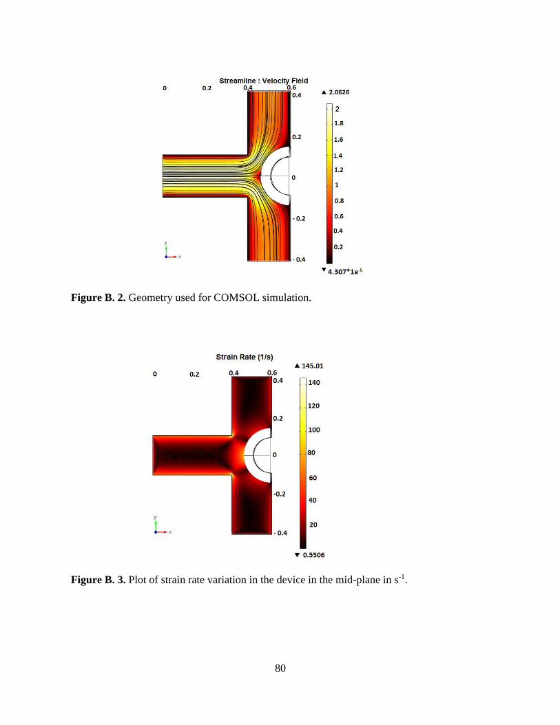
80
Figure B. 2. Geometry used for COMSOL simulation.
Figure B. 3. Plot of strain rate variation in the device in the mid-plane in s-1.

81
Stokes Number Stk was calculated to determine the effect of inertia on particles which
was defined as:
2
0Stk18
p p
d
d U
d
(B.4)
where, 𝑈𝑜 is fluid velocity far away from the drop, 𝑑𝑑 is diameter of drop. Substituting
as 1.05 g/cc, d as 10 μm , d as 100 μm, as 30 cP and U as 0.702 mm/sp p d o in Eq. (B.4), we get
6(10 ) 1Stk O . Therefore, the particle path line coincides with the flow streamlines. In other
words, particles never leave their streamlines.
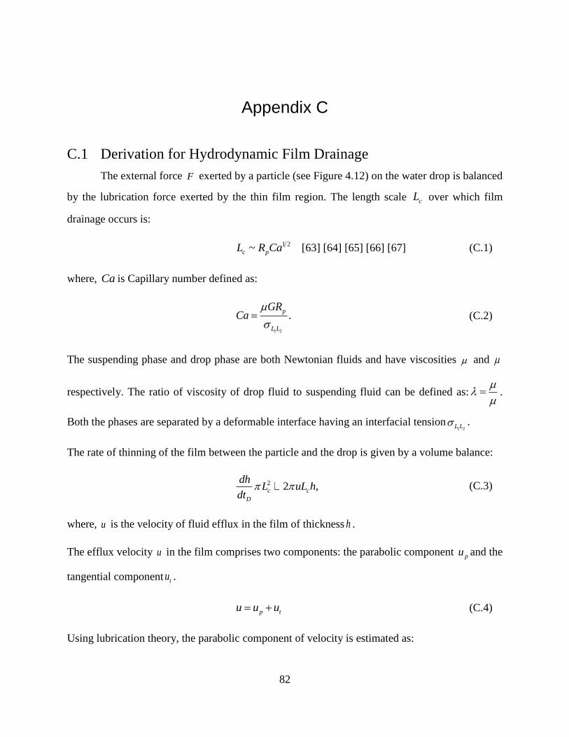
82
Appendix C
C.1 Derivation for Hydrodynamic Film Drainage
The external force F exerted by a particle (see Figure 4.12) on the water drop is balanced
by the lubrication force exerted by the thin film region. The length scale cL over which film
drainage occurs is:
1 2~c pL R Ca [63] [64] [65] [66] [67] (C.1)
where, Ca is Capillary number defined as:
1 2
.p
L L
GRCa
(C.2)
The suspending phase and drop phase are both Newtonian fluids and have viscosities and
respectively. The ratio of viscosity of drop fluid to suspending fluid can be defined as:
.
Both the phases are separated by a deformable interface having an interfacial tension1 2L L .
The rate of thinning of the film between the particle and the drop is given by a volume balance:
2 2 ,c c
D
dhL uL h
dt (C.3)
where, u is the velocity of fluid efflux in the film of thickness h .
The efflux velocity u in the film comprises two components: the parabolic component pu and the
tangential component tu .
p tu u u (C.4)
Using lubrication theory, the parabolic component of velocity is estimated as:
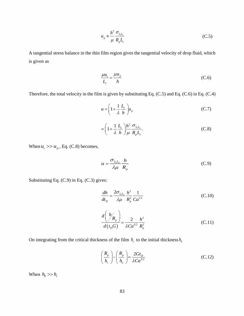
83
1 2
2L L
p
p c
hu
R L
(C.5)
A tangential stress balance in the thin film region gives the tangential velocity of drop fluid, which
is given as
pt
c
uu
L h
(C.6)
Therefore, the total velocity in the film is given by substituting Eq. (C.5) and Eq. (C.6) in Eq. (C.4)
11 c
p
Lu u
h
(C.7)
1 2
211 .
L Lc
p c
L h
h R L
(C.8)
When t pu u , Eq. (C.8) becomes,
1 2L L
p
hu
R
(C.9)
Substituting Eq. (C.9) in Eq. (C.3) gives:
1 2
2
2 1 2
2 1L L
D p
dh h
dt R Ca
(C.10)
2
3 2 2
2p
D p
hdR h
d t G Ca R
(C.11)
On integrating from the critical thickness of the film ch to the initial thickness 0h
3 2
2p p D
c o
R R Gt
h h Ca
(C.12)
When 0 ch h

84
3 2
t2
p
D
c
Ca R
Gh
(C.13)
C.2 Energy requirement for Bridge Formation Theory
The thermal fluctuations in the film causes the system to pass through an energy barrier
which leads to spontaneous film rupture and bridge formation at the point of contact. The particle
sticks to the drop by the formation of a liquid bridge from the drop phase. The bridge formed
would grow or contract based on a critical radius and energy of the system at this point is known
as the activation energy. Beyond the critical radius, the bridge grows spontaneously leading to
particle capture. The interface lost during bridge formation in the drop side results in a loss in the
free energy which depends on the contact cross sectional area and the interfacial tension between
the drop phase and the suspending fluid (see Figure 4.14). The free energy penalty 1E in the drop
side is defined as:
1 2
2
1 C L LE r (C.14)
where, Cr is bridge radius and 1 2L L is interfacial tension between drop phase and suspending phase.
The reduction in free energy in drop side results in a gain in free energy 2E in the planar film
region which is written as:
1 22 2 C L LE r h (C.15)
where, h is film thickness.
On the other hand, there is initially a free energy penalty on the particle surface and eventually a
free energy gain in particle side due to an increase in energy in the film region.
2 1
2
3 ( )C L S L SE r (C.16)
where,1L S is interfacial tension between drop phase and particle and
2L S is interfacial tension
between suspending phase and particle.

85
The change in free energy E is:
2 1 1 2 1 2
2( ) 2C L S L S L L C L LE r r h (C.17)
The relationship between Cr and h can be found by differentiating Eq. (C.17) with respect to Cr
and equating it to 0.
2 1
1 2
1
C
L S L S
L L
hr
(C.18)
Where, 2 1
1 2
L S L S
L L
is three phase contact angle defined as cos θ . In our case, since the particle
is water-wetting, cos is defined with respect to drop phase. Hence, Eq. (C.18) is rewritten as:
1 cosC
hr
(C.19)
Thus, the energy required for transition from state 1 to state 2 in Figure 4.14 is
1 2
2
.1 cos
L L hE
(C.20)
The rest of the details on the bridge formation time scale is mentioned in section 4.2.1 of
Chapter 4.

86
Contribution
I would like to thank Professor Edgar Acosta and Professor Eugenia Kumacheva for granting me
permission to use their lab equipment such as goniometer, force Tensiometer, swinging bucket
centrifuge and plasma cleaner respectively. I acknowledge the Centre for Microfluidics and TNFC
at University of Toronto for the fabrication facilities. I thank Dr. Thomas Leary for sharing his
figure on particle capture for high capillary numbers. I also thank Willam Wang for helping me in
understanding image processing in Matlab. A special word of thanks to Rohit Sonthalia for coming
up with the alternative design of the microfluidic aspiration device and performing coalescence
experiments in it. I also acknowledge ACS PRF for funding my project.