research article vibration control by means of piezoelectric...
TRANSCRIPT

Research ArticleVibration Control by Means of Piezoelectric Actuators Shuntedwith LR Impedances Performance and Robustness Analysis
M Berardengo1 A Cigada1 S Manzoni1 and M Vanali2
1Department of Mechanical Engineering Politecnico di Milano Via La Masa 34 20156 Milan Italy2Department of Industrial Engineering Universita degli Studi di Parma Parco Area delle Scienze 181A 43124 Parma Italy
Correspondence should be addressed to S Manzoni stefanomanzonipolimiit
Received 29 October 2014 Revised 8 April 2015 Accepted 14 April 2015
Academic Editor Lei Zuo
Copyright copy 2015 M Berardengo et alThis is an open access article distributed under the Creative Commons Attribution Licensewhich permits unrestricted use distribution and reproduction in any medium provided the original work is properly cited
This paper deals with passive monomodal vibration control by shunting piezoelectric actuators to electric impedances constitutingthe series of a resistance and an inductance Although this kind of vibration attenuation strategy has long been employed there arestill unsolved problems particularly this kind of control does suffer from issues relative to robustness because the features of theelectric impedance cannot be adapted to changes of the system This work investigates different algorithms that can be employedto optimise the values of the electric components of the shunt impedance Some of these algorithms derive from the theory of thetuned mass dampers First a performance analysis is provided comparing the attenuation achievable with these algorithms Thenan analysis and comparison of the same algorithms in terms of robustness are carried out The approach adopted herein allowsidentifying the algorithm capable of providing the highest degree of robustness and explains the solutions that can be employed toresolve some of the issues concerning the practical implementation of this control technique The analytical and numerical resultspresented in the paper have been validated experimentally by means of a proper test setup
1 Introduction
Mitigation of vibrations in structures is a crucial issue inseveral fields such as electronics automotive space andmanufacturing It can lead to higher quality products itimproves durability by protecting components from fatigueand failure it achieves reduced maintenance costs and itimproves comfort to people in terms of noise and vibration
In this scenario the control of light structures is of par-ticular importanceMany industrial and engineering applica-tions indeed rely on lightweight structures subject to a harshdynamic environment Usually these structures have lowdamping values thus the vibration level induced can be veryhigh Furthermore they are lightweight so that the actuatorsused for control purposes often introduce high load effects
Due to these issues many active and passive strategieshave been developed to increase the damping of thesestructures Among the passive strategies up to 20 years agothe most common were the introduction of high loss factorviscoelastic materials within the structure or connection to
a mechanical vibration absorber In 1991 Hagood and vonFlotow [1] proposed a new method to passively increasethe structural damping by relying on piezoelectric materialsshunted to a proper electrical network Since this advance avariety of passive and semipassive vibration reduction tech-niques based on piezoelectric materials have been proposed
The capability of piezoelectric materials to convertmechanical energy into electrical and vice versa can indeedbe employed in different ways they can be used as sensorsor actuators for active and passive control strategies Asregards the passive or semipassive control techniques thesematerials allow either dissipating or reusing the electricalenergy induced by the mechanical deflection by means ofa suitable electrical device In the latter case an electricalnetwork has to be properly designed and shunted to a piezo-actuator in order to generate an action opposite to themotionof the hosting structure
The simplest passive shunt-circuits for single mode con-trol are the resistive (119877) and the resistive-inductive (119871119877 orresonant shunt in which a resistance and an inductance are
Hindawi Publishing CorporationShock and VibrationVolume 2015 Article ID 704265 30 pageshttpdxdoiorg1011552015704265
2 Shock and Vibration
connected in series) which are the electrical equivalents ofa Lanchester damper and a Tuned Mass Damper (TMD)respectively [2 3] Such network layouts are widely used fortheir effectiveness In addition to these circuits other typesof shunt impedance have been developed among others Wu[4] has suggested using a resistance and an inductance inparallel and Park and Inman [5] studied together both seriesand parallel 119871119877 circuits
These passive techniques based on shunted piezoelectricactuators are particularly appealing to the scope of suppress-ing vibration they require no power to be effective whicheven allows coupling them to energy harvesting systemsMoreover they cause little additional weight a strategic issuefor most light structures (eg space structures) Further-more these methods do not require either digital or analogexpensive control systems and feedback sensors they arealways stable and easy to implement On the other hand theseapproaches are less flexible than active control strategiestherefore they must be carefully designed and optimised foreach specific application It is also noticed that 119877 and 119871119877
impedances can be coupled to a negative capacitance [6ndash8] in order to increase their attenuation performances Suchan approach allows increasing the vibration attenuation pro-vided by the shunt impedance but poses some issues relatedto the stability of the electromechanical system becausea circuit based on operational amplifiers is used to buildthe negative impedance Therefore the shunt impedancebecomes semiactive
Several strategies have been suggested to optimize theimpedance parameters so to achieve the best performancesfrom single mode controllers Hagood and von Flotow [1]proposed tuning strategies based on transfer function criteriaand on pole placement to tune the numerical values of the119877119871shunt impedance in undamped structures Both these tuningmethods are based on the classic TMD theory given that the119877119871 circuit is the electrical equivalent of the TMD In the firstmethod abovementioned that is transfer function criterionthe inductance value is found by imposing some constraintson the transfer function shape of the coupled system Insteadin the latter pole placement technique the resistance andinductance values are set so that the complex poles of theshunted piezoelectric system reach the leftmost excursionin the s-plane Hoslashgsberg and Krenk developed a balancedcalibration method for series and parallel 119877119871 circuits basedon pole placement [9] In this case the 119877 and 119871 values arechosen in order to guarantee equal modal damping of thetwo modes of the electromechanical structure and thus goodseparation of complex poles This option guarantees a goodcompromise between high damping and performance interms of response reductionwith limited damping Successfulempirical methods to tune the 119877119871 impedance [10] have alsobeen proposed in order to optimize the performance of thesystem only with knowing the geometric mechanical andelectrical characteristics of the hosting structure and actuator
In addition to the impedance optimization several stud-ies have investigated the influence of the geometry andplacement of the piezoelectric actuator on the performancesof the controller A number of studies to optimize geometryand position of the piezo-actuator have been carried out on
the basis of finite element model analysis [11ndash14] InsteadDucarne et al proposed a method to optimise the geometryand the placement of the piezo-actuator in order to increasethe damping efficiency by maximizing the Modal Electro-Mechanical Coupling Factor (MEMCF) [15] Thomas et alalso proposed closed formulas to evaluate the performanceof the controller as function of the MEMCF [16]
For several reasons the performances of these passivecontrol strategies are lower than the ones employing activecontrol even though they are optimized so to achieve thebest vibration attenuation firstly the power involved in thecontrol is lower than in the case of active control secondly theabsence of a feedback control linked to an error signal doesnot allow improving control performance during actuationConsequently these strategies are much more conditionedby the uncertainties and sensitive to the changes of theparameters involved thus leading to poor results when thestrategies are not well tuned to the specific applicationTherefore in most cases it is not possible to successfullyapply the methods available in literature in order to choosethe right values of the impedance parameters In most ofthe cases the practical applications require empirical tuningor adjustment of the theoretical optimal values This is inagreement with the results obtained byThomas et al in theirexperimental tests [16] In fact they had to adjust the theoret-ical values calculatedwith their optimizationmethod in orderto achieve the highest attenuation values The uncertaintywhich affects the mechanical and electrical parameters ofboth the structure and the piezoelectric actuators is indeedextremely high in the practical application Furthermoremistuning can occur even when starting from a perfectlytuned condition for instance if the environmental tempera-ture changes the eigenfrequency of the system to control willshift and a mistuning will thus occur Therefore the chancesof having to work in mistuned conditions are very high inpractical cases and this causes worse vibration attenuationperformance
Some techniques based on adaptive circuits have beenproposed to overcome the limitations due to uncertainty onmechanical and electrical quantities leading to mistuning Asregarding the single mode control Hollkamp and Starchvilledeveloped a self-tuning119877119871 circuit able to follow any change infrequency of themode to control [17]This technique is basedon a synthetic circuit (which provides both the inductanceand the resistance of the circuit) constituted by two opera-tional amplifiers and a motorized potentiometer A changeof the input voltage to the motorized potentiometer resultsin a change of the electrical resonance so that the controlsystem can follow themechanical resonance change allowingthe correct tuning of the impedance Nevertheless this circuitcontains active components needing a power supply thus thisstrategy cannot be considered passive Furthermore the onlyuncertainty taken into consideration in the abovementionedreferenced work is the one relative to the frequency of thecontrolled mode while the uncertainty relative to the shuntparameters and to the electrical quantities of the piezo-actuator is not taken into account Other recent works byZhou et al investigated methods to limit the problem ofmistuning by binding more than one piezo-actuator to
Shock and Vibration 3
the vibrating structure [18] and by employing nonlinearelements when the disturbance is harmonic [19]
Although the passive control strategies bymeans of piezo-electric actuators have been widely studied in the last twentyyears there is still much need for improvement because ofsome criticalities The most relevant ones are summarizedbelow and will each be discussed in detail further in thissection
(1) Most of the methods to tune the shunt impedanceavailable in literature require the estimation of thenatural frequency of the electromechanical systemin open and short circuit conditions or the esti-mation of the Electro-Mechanical Coupling Factor(EMCF)
(2) In most cases the impedance optimization algo-rithms provide numerical values of the parameterswhich are nonetheless unfeasible in practice As for119877119871 tuning very large inductors are necessary for themore commonplace mechanical frequencies more-over the resistance values are often so small that thesole resistance of the cables and of the piezo-actuator[20] together results to be higher than the value ofthe optimal shunt resistance itself Therefore it isnecessary to implement synthetic circuits bymeans ofoperational amplifiers in order to overcome the lim-itation due to the high value of the inductance 119871 Thissolution nonetheless leads to the problem that thissynthetic circuit requires power supplyMoreover theproblem of the low value of the resistance has seldombeen studied in literature
(3) Although it is well known [21ndash23] that the perfor-mance of the control strategy varies significantly incase of uncertainty on the mechanical and electricalparameters of both structure and actuator a robust-ness analysis has not yet been carried out in anyof the works available in literature Furthermorethe behaviour of the optimisation methods in caseof mistuning has never been analysed in terms ofattenuation performances
The aim of this paper is thus to resolve some of these short-comings
Relative to the issue in point 1 of the list presentedabove the problem should be broken down into differentconsiderations Firstly when a numerical estimate of theEMCF value is needed approximated closed formulas maybe used when available [15] or else it is possible to measurethe natural frequency of the short and open circuit In thislatter case the piezo-actuator has to be chosen and bondeda priori and only subsequently the impedance can be tunedTherefore the optimization procedure is carried out in twodifferent steps the optimization of the actuator placementand the optimisation of the impedance parameters Thoughsome optimization methods are available for the placementand the geometry of the actuator [11ndash15] this procedureprecludes the possibility to perform a more general analysistaking into account at the same time the shunt-impedanceparameters the geometric parameters and the position of
the actuator But such an analysis can be of great importancefor a number of reasons a specific desired performance maybe achieved by different configurations not necessarily theoptimum one Moreover sometimes a solution comparableto the optimal one in terms of vibration reduction can also beachieved with an electromechanical configuration differentfrom the optimal one in terms of geometry and position of theactuator by properly tuning the impedance parameters Thissolution can be hardly achieved if the optimization is carriedout in two separate steps A comprehensive analysis in whichevery parameter is optimized at the same time would alsoallow to estimate the performance of the controller a prioriand therefore to highlight whether such a kind of controlstrategy can be effective enough or not
The second point in the list of criticalities abovemen-tioned concerns the values of 119877 and 119871 deriving from theoptimization methods the problem is that their values oftenresult to be too small and too large respectively in order tobe obtained by physical passive componentsThis leads to theneed of implementing the impedance through operationalamplifiers in turn requiring power supply even though thepower necessary is actually very low The comprehensiveapproach proposed above could clarify if the values of 119877 and119871 can be changed in order to become feasible by changingother system parameters (eg geometric mechanical andelectrical parameters position of the actuator) maintainingthe same performance of the controller
By combining this general analysis with an analysisof robustness to mechanical and electrical uncertaintiesproposed in point number 3 of the list of criticalities a clearerand complete insight on the problem under analysis can beachieved
This paper proposes an analytical treatment that enablesthe user to investigate all these aspects A comprehensiveapproach as discussed above has been developed it aims atobviating to the aforementioned criticalities by sustaining thetuning algorithm by means of a performance and robustnessanalysis
The model employed to describe the dynamic behaviourof the coupled electromechanical system plays an importantrole in the development of this procedure It must provideclear formulations which allow performing a global analysishighlighting simultaneously the influence of the positionof the piezo-actuator of its geometry and of the shuntimpedance parameters Then all the analyses underlinedbefore can be carried out
This model chosen takes advantage of the one proposedby Moheimani and Fleming [3] and has several benefitsFirstly the control action performed by the shunted electricalnetwork is seen as a feedback loop this allows applyingthe classic control theory to the electromechanical systemMoreover this model is able to describe at the same timethe behaviour of both the elastic structure and the piezo-electric actuator which in turn are coupled with the shuntedimpedance This kind of modelling takes into account boththe electromechanical structure (piezoactuator + structure)and the shunt impedance Also this model can describe witha single mathematical description both 1-dimensional (egbeams) and 2-dimensional (eg plates) structures
4 Shock and Vibration
Cp
V = minusVpminusVp
(a)
minusVp
Structure
Piezo
(b)
Figure 1 Electric equivalent of a piezoelectric actuator (a) bonded to an elastic structure (b)
By the use of this analytical model this paper demon-strates that there is one specific parameter which affects thecontrol performances and the effectiveness of the controlstrategy Such a parameter depends only on the mechanicalgeometrical and electrical characteristics of the structureand of the actuator This parameter together with the shuntimpedance parameters can be then modified and properlytuned in order to achieve the target performances Asexplained above the simultaneous tuning of these parameterscan be advantageous Furthermore this approach brings tolight the ineffectiveness of the control techniques based onshunted piezoelectric actuators in the cases where the naturalfrequencies and the damping of the mode to be controlledexceed given values
In this scenario three different methodologies to tune theimpedance parameters have been developed all relying ontransfer function considerations Analytic closed formulas toderive the optimal values of the resistance and inductance ofthe 119877119871 shunt circuit for damped light structures were thenderived Although all of these strategies prove to be veryeffective when there are no uncertainties on the parametersa robustness analysis shows that one of these three tuningalgorithms is more robust than the others to uncertainties onelectrical and mechanical parameters
All the results have been experimentally validated Sincethe approach developed in this paper results is valid for bothbeams and plates the authors have decided to build a testsetup with an aluminium plate and a piezo patch bondedclose to its centre which provides a more complex case-studythan those commonly treated in literature (ie often the 1-dimensional case is preferred)
This paper is structured as follows The general elec-tromechanical model for an elastic structure with piezoelec-tric elements coupled to an electric circuit is described inSection 2The three different tuning methodologies based ontransfer function considerations are presented in Section 3and analytic formulas to tune 119877 and 119871 are derived Section 4illustrates the performance analysis of the mentioned opti-misation methods and explains the effect of the electric andmechanical characteristics of the structure and of the piezo-actuator on the 119877 and 119871 values The robustness analysis ofthe optimization methods is presented in Section 5 FinallySection 6 illustrates and explains the experimental tests car-ried out on a plate and a simplified formulation for the mostrobust tuning procedure is proposed in Section 7
2 Electromechanical Model
This section treats the analytical modelling of the whole elec-tromechanical structure constituted by the elastic structurethe piezo-actuator and the shunting impedance Thoughsome of the issues treated in this section are already knownand discussed in literature [3 24 25] the authors havedecided to provide a concise recapitulation of them forsake of clarity such an abridgement is moreover meant tomake the paper more readily accessible and makes for abetter understanding of the improvements contributing tosuch a model by this paper This section is subdivided intofour parts the first part describes the electric model of thepiezoelectric actuator is described part two highlights thefeedback nature of the controlled system and the third partprovides the dynamic model of the coupled system andanalytical formulations are derived for cases that have yet tobe analysed in literature Finally this model is used to achievea new formulation of the frequency response function of thecontrolled structure in the fourth subsection
21 Electric Equivalent Scheme of a Piezoelectric ActuatorPiezoelectric materials are materials such that an appliedstress is capable of generating a charge on the surfaces ofthe piezoelectric element and an applied voltage generatesa strain Thanks to the latter working principle the shapeof the solid can be modified depending on the chargeinduced on the surfaces of the piezoelectric element Thesetwo effects (called piezoelectric effects direct and inverseresp) entail to employ these materials as both sensors andactuators making them extremely interesting in applicationsfor vibration control
One of the models which can be used to describe theelectrical behaviour of piezoelectric materials is a series of acapacitor 119862119901 and a strain-dependent voltage generator minus119881119901[26] as shown in Figure 1
Two piezoelectric patches are usually needed to controla light structure by means of piezoelectric materials oneacting as sensor and the other as actuator (Figure 2) Thesensor output (ie the voltage119881 across the piezoelectric patchelectrodes) is equal to minus119881119901 (Figure 1) and it depends on thestrain of the structure to which it is bonded In turn thisvoltage is the input to the controller which uses this signal asthe reference for its control law generating an output voltage
Shock and Vibration 5
Actuator
Sensor
(a)
Actu
ator
Sens
or
K
V minusVp
(b)
Figure 2 Scheme of an elastic structure controlled by means of coupled piezoelectric sensor and actuator
Z
Structure
Piezo
(a)
Z V
minusVp
Cp
(b)
Figure 3 Scheme of a structure controlled by a shunted piezo-actuator (a) and its electrical equivalent (b)
119881 applied to the piezo-patch acting as actuator This piezo-actuator will thus change its shape thus applying a controlforce to the structure
The control mechanism described here can also be madeby using a single piezo-patch which behaves at the sametime as sensor and actuator In this case a single piezoelectricelement is shunted to an impedance 119885 [3] (Figure 3) thestructure vibration will induce a voltage 119881 to the terminalsof the actuator (equal to minus119881119901 when the circuit is opensee Figure 1) Since the impedance 119885 is connected to thepiezoelectric element a current 119894119911 circulates and the voltage119881 between the terminals of the impedance119885will no longer beminus119881119901 but it will bemodified by the presence of the impedanceThis voltage becomes the input to the piezo-element and thusinduces a change of the strain of the patch (ie a control forceis imposed to the structure) Hence the voltage 119881 and thecontrol action to the structure depend on how the impedanceused to shunt the actuator is built Thus its layout and thevalues of its parameters must be carefully chosen accordingto the specific application in order to maximize the controleffect
This kind of control scheme (Figure 3) is chosen todevelop the single mode control strategies presented in thispaper
22 Feedback Representation of the Control by Means of aShunted Piezoelectric Actuator Taken here into considera-tion is a structure controlled by a piezoelectric actuatorshunted by an impedance 119885 and subject to the disturbance119882 (Figure 4(a)) and its electrical equivalent as shown inFigure 4(b) The disturbance 119882 induces a flexural motionof the elastic structure described by the variable 119911 whichrepresents the transversal displacement As explained in[27] if the impedance 119885 is removed (open circuit) thevoltage 119881 at the terminals of the actuator results equals minus119881119901(Figure 1(b)) and is entirely induced by the strain generatedby the disturbance 119882 In this case the voltage minus119881119901 can berelated to the disturbance119882 by the transfer function 119866V119908
minus119881119901 (119904) = 119866V119908119882(119904) (1)Otherwise in the case no disturbances act on the structureand the impedance 119885 is replaced by a voltage source 119881
6 Shock and Vibration
Actuator
W
z
y
(a)
iz
Z
V
V
c Cp
minusVp
(b)
Figure 4 Structure controlled by a piezoelectric actuator shunted by the impedance 119885 and subject to the disturbance119882 (a) and its electricalequivalent (b)
then minus119881119901 depends only on the voltage 119881 Thus the relationbetween119881 and minus119881119901 can be expressed by the transfer function119866VV
minus119881119901 (119904) = 119866VV119881 (119904) (2)
When the disturbance 119882 acts on the structure and thevoltage 119881 is applied to the terminals of the piezo-actuatorthe voltage minus119881119901 can be expressed as the sum of the twocontributions because of the linearity of the system Byapplying the superposition principle it is then possible towrite
minus119881119901 (119904) = 119866VV119881 (119904) + 119866V119908119882(119904) (3)
As for Figure 4(b) the following expressions are achieved byapplying the Kirchhoff and the Ohm laws
119881119888 = minus119881119901 minus 119881
119881 = 119885119894119911
(4)
where 119881119888 = 119894119911119862119901119904 in the Laplace domainEquations (3) and (4) allow representing the electrome-
chanical structure constituted by the elastic structure thepiezo-patch and the impedance as the feedback controlledsystem in Figure 5 where the controller 119870 in the Laplacedomain is represented by the inner loop
119870 (119904) =119881
minus119881119901
=
119904119862119901119885
1 + 119904119862119901119885 (5)
Therefore the impedance 119885 can be used to produce a givenvoltage 119881 capable of reducing the effect induced by thedisturbance119882 The impedance used in this paper to developa single mode control strategy is constituted by a resistance 119877in series with an inductance 119871
As mentioned above different tuning methodologies willbe defined in Section 3 in order to choose the optimal valuesof the impedance parameters (ie 119877 and 119871) relying on
+ +
+
++
0 sCp Z(s) G(s)V
Gw(s)
W
minusVpminus
K(s)
iz
Figure 5 Feedback representation of the controlled structure
transfer function considerations The selected target transferfunction shall allow describing the response of the elasticstructure in terms of deflection to an external disturbanceTherefore the expression of the closed loop transfer function119879119911119908 between the disturbance119882 and the displacement 119911 of thestructure is needed
As for Figure 5 the closed loop transfer function 119879V119908relating the voltage minus119881119901 with the disturbance 119882 can bedefined as
minus119881119901 = 119866V119908119882+ 119866VV119881
997904rArr minus119881119901 = 119866V119908119882+ 119866VV119870(minus119881119901)
997904rArr 119879V119908 =
minus119881119901
119882= 119866V119908
1
1 minus 119870119866VV
(6)
Once the transfer function 119866 between the voltage 119881 and thedisplacement 119911 (ie 119866(119904) = 119911119881) is defined 119879119911119908 can beexpressed as
119879119911119908 =119911
119882= 119879V119908
119866
119866VV= 119866V119908
1
1 minus 119870119866VVsdot1
119866VV119866 (7)
Thus the analytic expressions of 119866 119866VV and 119866V119908 must beknown in order to derive the expression of 119879119911119908 and thus thedynamics of the coupled system (ie piezo-actuator + elasticstructure) must be taken into account
Shock and Vibration 7
z
y
x
y1
y2
x1x2
Mx
Mx
MyMy
tp
h
b
a
Figure 6 Plate structure with a piezo-element
23 Dynamic Model of the Electromechanical System Themathematical procedure developed in this section to derivethe analytic relations between the electric and mechanicalquantities involved in this control problem (ie 119881 minus119881119901 119911and 119882) is referred to a plate structure (Figure 6) This sameapproach can be used to derive these relationships for one-dimensional cases (ie beam structures) as well [24 25] Theauthors have decided to refer to the two-dimensional case butto report only the final results for the one-dimensional casefor sake of conciseness and because the experimental tests(Section 6) were performed on a plate
The analytical formulation of the transfer functions 119866119866VV and 119866V119908 can be achieved by employing the expressionswhich relate the voltage induced at the terminals of the piezo-patch in open circuit (ie minus119881119901) to its deformation and theequations of motion of the electromechanical system [3 24]
The first of these equations (ie the relation between thevoltage induced at the terminals of the piezo-patch in opencircuit minus119881119901 and its deformation) can be derived consideringthat the voltage between the piezo-actuator terminals minus119881119901in open circuit can be expressed as function of the charge 119902induced on the surfaces of the patch
minus119881119901 =119902
119862119901(8)
and the charge 119902 can be obtained as the surface integral of theelectric displacement in 119911 direction named1198633
119902 = int119860119901
1198633119889119860119901 (9)
where 119860119901 is the surface of the piezoelectric patch From theequation describing the direct piezoelectric effect [3] theexpression of the electric displacement 1198633 can be derivedas function of the stresses on the piezo-patch in 119909 and119910 directions (120590119901
119909and 120590
119901
119910) and of the piezoelectric strain
constants 11988931 and 11988932
1198633 = 11988931120590119901
119909+ 11988932120590
119901
119910 (10)
Assuming the piezoelectric material bears similar propertiesin 119909 and 119910 directions the two piezoelectric constants canbe considered equal 11988932 = 11988931 Furthermore the stresses
(120590119901119909 120590119901
119910) and strains (120576119875119909 120576119875119910) in the piezoelectric patch in
open circuit can be described by the following expressions
120590119901
119909=
119864119901
1 minus ]2119901
(120576119875119909+ ]119901120576119875119910)
120590119901
119910=
119864119901
1 minus ]2119901
(120576119875119910+ ]119901120576119875119909)
120576119875119909= (
ℎ
2+
119905119901
2)1205972119908
1205971199092
120576119875119910= (
ℎ
2+
119905119901
2)1205972119908
1205971199102
(11)
where ℎ and 119905119901 are the thickness of the plate and of the piezo-actuator respectively 119864119901 and ]119901 are Youngrsquos and Poissonrsquosmoduli of the piezo-patch and 119908 is the transverse deflectionof the coupled structure
By substituting (9) (10) and (11) in (8) the relationbetween the deformation of the piezoelectric patch and thevoltage induced at its terminals is derived
minus119881119901 =
11986411990111988931 (ℎ + 119905119901)
2119862119901 (1 minus ]119901)int
1199102
1199101
int
1199092
1199091
(1205972119908
1205971199092+1205972119908
1205971199102)119889119909119889119910 (12)
where 1199091 1199092 1199101 and 1199102 are the coordinates of the actuatorextremities (Figure 6)
Now that the first equation has been derived (ie therelation between the voltage induced at the terminals of thepiezo-patch in open circuit minus119881119901 and its deformation) theequations of motion of the plate are necessary to calculate thetransfer functions 119866 119866VV and 119866V119908
As explained in the previous section 119866 119866VV and 119866V119908represent the transfer functions related to the cases in whicheither the disturbance 119882 or the applied voltage 119881 is actingon the system This means that the response of the elasticstructure to the forces induced by the applied voltage 119881 andthe disturbance 119882 separately must be known in order tocalculate these transfer functions
The dynamic equation of a plate subject to a forcingterm 119882 is represented by the following Partial DifferentialEquation (PDE) [28]
120588ℎ1205972119908
1205971199052+ 119863nabla
4119908 (119909 119910 119905) = 119882 (13)
where 120588 is the density of the plate material and
nabla4119908 =
1205974119908
1205971199094+ 2
1205974119908
12059711990921205971199102+1205974119908
1205971199104
119863 =119864ℎ
3
12 (1 minus ]2)
(14)
where ] and119864 are Poissonrsquos coefficient and Youngrsquos coefficientof the plate material respectively Equations (13) and (12)expressed in modal coordinates and represented in Laplace
8 Shock and Vibration
120572
z
x
(a)
120572
z
y
(b)
Figure 7 Two-dimensional strain distribution of a plate with two antisymmetric colocated piezoelectric elements (a) 119911-119909 plane and (b) 119911-119910plane
domain allow calculating the transfer function 119866V119908 betweenthe voltage minus119881119901 and the disturbance119882
119866V119908 =
minus119881119901
119882=
11986411990111988931 (ℎ + 119905119901)
2119862119901 (1 minus ]119901)
infin
sum
119896=1
Φ119896 (119909119865) 120595119896
1199042 + 2120585119896120596119896119904 + 1205962
119896
(15)
where 120596119896 is the 119896th eigenfrequency of the plate and 120585119896 isthe associated nondimensional damping ratio Φ119896 is the 119896theigenmode (normalised to unit modal mass) of the plateΦ119896(119909119865) represents the value of the 119896th mode at the forcingpoint 119909119865 and 120595119896 for the two-dimensional case is
1205951198962119863 = int
1199102
1199101
120597Φ119896 (119909 119910)
120597119909
100381610038161003816100381610038161003816100381610038161003816119909=1199092
119889119910
minus int
1199102
1199101
120597Φ119896 (119909 119910)
120597119909
100381610038161003816100381610038161003816100381610038161003816119909=1199091
119889119910
+ int
1199092
1199091
120597Φ119896 (119909 119910)
120597119910
100381610038161003816100381610038161003816100381610038161003816119910=1199102
119889119909
minus int
1199092
1199091
120597Φ119896 (119909 119910)
120597119910
100381610038161003816100381610038161003816100381610038161003816119910=1199101
119889119909
(16)
where 120595119896 is a term dependent on the curvature of the 119896thmode and assumes different formulations for 1D or 2D casessee Table 1 (the other parameters in Table 1 are explained inthis section further on)
As for 119866 and 119866VV the forcing term of (13) has to bereplaced by the forcing action generated on the structureby the piezo-actuator The equation governing the dynamicof the plate subject to the moments applied by the piezo-actuator can be described by the following PDE [28]
120588ℎ1205972119908
1205971199052+ 119863nabla
4119908 (119909 119910 119905) =
1205972119872119909
1205971199092+
1205972119872119910
1205971199102 (17)
where themoments per unit length119872119909 and119872119910 represent theforcing term due to the piezoelectric patch (Figure 6)
The forcing term must be defined in order to solve thedynamic equation (17) to make explicit the dependency ofthe moments on the voltage 119881 and to calculate 119866 and 119866VV
The flexural moment applied to the structure is due tothe deformation of the piezo-patch caused by the voltage
119881 applied to its terminals Thus the expression linking thevoltage applied to the terminals of the piezoelectric patchand the moments generated must be derived For sake ofthoroughness this paper explains the procedure to obtain thisterm because for some particular cases (illustrated further onin this section) the available literature does not elucidate theresults but is limited to suggesting the procedure to obtainthem
The moments acting on the plate can be described by thefollowing expression
119872119901119909 = minusint119860119909
119911120590119909119889119860119909
119872119901119910 = minusint119860119910
119911120590119910119889119860119910
(18)
where 120590119909 and 120590119910 are the stresses acting on the plate in 119909 and119910 directions and 119860119909 and 119860119910 are the transverse cross-sectionsof the plate (ie 119860119909 = 119887ℎ and 119860119910 = 119886ℎ referring to Figure 6)
The system represented in Figure 7 with two colocatedpiezoelectric actuators and a phase of 180∘ between the twoof them shall be discussed now Relying on the hypothesisof a homogeneous plate the strain in 119909 and 119910 directions canbe considered the same and equals 120576119909 = 120576119910 = 120576 = 120572119911 (seeFigure 7) The stresses in the plate and in the piezo-actuatorscan be expressed as
Plate
120590119909 =119864
1 minus ]2(120576119909 + ]120576119910)
997904rArr 120590119909 = 120590119910 =119864
1 minus ]2(1 + ]) 120576
120590119910 =119864
1 minus ]2(120576119910 + ]120576119909)
Piezo
120590119875
119909=
119864119875
1 minus ]2119875
(120576119909 + ]119875120576119910 minus (1 + ]119901) 120576119875)
119875
119909=
119864119875
1 minus ]2119875
(120576119909 + ]119875120576119910 + (1 + ]119901) 120576119875)
120590119875
119910=
119864119875
1 minus ]2119875
(120576119910 + ]119875120576119909 minus (1 + ]119901) 120576119875)
119875
119910=
119864119875
1 minus ]2119875
(120576119910 + ]119875120576119909 + (1 + ]119901) 120576119875)
(19)
where the symbol sim refers to the stresses in the actuatorat the bottom In (19) the piezoelectric actuator is assumedto have the same properties in 119909 and 119910 direction and
Shock and Vibration 9
Table1Ex
pressio
nsto
calculate119870
120574and
120595119896for
the1-and
2-dimensio
nalcasesw
here119905119887isthethicknessof
theb
eam119864
119887istheY
oungrsquosmod
ulus
oftheb
eam
materialand119868119887isthem
oment
ofinertia
oftheb
eam
Parameter
Beam
Plate
119870minus11986411988711986811988712059411988931
119905119901
minus119864119868
(1minus])12059411988931
119905119901
120574119870
11986411990111988931119908119901(119905119887+119905119901)
2119862119901
119870
11986411990111988931(ℎ+119905119901)
2119862119901(1minus] 119901)
120595119896
1205951198961119863=Φ1015840 119896(1199092)minusΦ1015840 119896(1199091)
1205951198962119863=int
1199102
1199101
120597Φ119896(119909119910)
120597119909
1003816 1003816 1003816 1003816 1003816 1003816 1003816 1003816 119909=1199092
119889119910minusint
1199102
1199101
120597Φ119896(119909119910)
120597119909
1003816 1003816 1003816 1003816 1003816 1003816 1003816 1003816 1003816 119909=1199091
119889119910+int
1199092
1199091
120597Φ119896(119909119910)
120597119910
1003816 1003816 1003816 1003816 1003816 1003816 1003816 1003816 1003816 119910=1199102
119889119909minusint
1199092
1199091
120597Φ119896(119909119910)
120597119910
1003816 1003816 1003816 1003816 1003816 1003816 1003816 1003816 119910=1199101
119889119909
10 Shock and Vibration
=
+
x
x x
z
zz
120572z 1205760
Figure 8 Asymmetric strain condition of a plate with a single actuator configuration
the unconstrained strain of the piezoelectric actuator due toan applied voltage is given by
120576119875119909= 120576119875119910
= 120576119901 =11988931
119905119901
119881 (20)
The expression of the coefficient 120572 describing the deforma-tion in the plate (Figure 7) must be derived to calculate theanalytic expressions of the stresses in the plate which in turnare necessary to calculate the moments Such an expressioncan be computed by applying the moment equilibrium in 119909
and 119910 directions [3 24 25]
int
ℎ2
minus(ℎ2)
120590119909119911 119889119911 + int
1199052+119905119901
1199052
120590119875
119909119911 119889119911 = 0
int
ℎ2
minus(ℎ2)
120590119910119911 119889119911 + int
1199052+119905119901
1199052
120590119875
119910119911 119889119911 = 0
(21)
Just one of the two equilibria can be taken into considerationto derive the expression of 120572 since the plate is assumed to behomogeneous (ie 120590119909 = 120590119910 = 120590 and 120590119875
119909= 120590
119875
119910= 120590
119875)Equation (21) shows that the value of the coefficient 120572
changes according to the stresses in the plate (ie 120590 =
119864120576 = 119864120572119911) In turn the stress distribution depends on thelayout of the electromechanical structureThemost commonconfigurations for this kind of problem are antisymmetric orasymmetric The antisymmetric configuration is constitutedby two colocated actuators or by colocated sensor-actuatorpair In the antisymmetric configuration instead a singlepiezo-electric element acting as an actuator is bonded to thestructure The expression of the coefficient 120572 in the asym-metric configuration for a plate has not yet been discussedin its explicit formulation in existing literature moreover thisis the configuration for the plate control by means of shuntedpiezo-actuators thus the authors have derived its formulation(see Table 2) and employed it in the herein paper The straincondition in the plate is asymmetric with this layout andcan be decomposed in two parts flexural and longitudinal(Figure 8) The equilibria of moments and axial forces mustbe imposed to calculate 120572 and 1205760 see Figure 8
The expressions of 120572 for all the abovementioned configu-rations for both beams and plates are listed in Table 2
As for the expressions of 120572 in Table 2 it is opportune toexpress 120572 as 120572 = 120594120576119901 in the following formulations
The value of 120572 has been derived so the moment acting onthe plate119872119901119909 can be computed by substituting (19) into (18)
119872119901119909 = minusint119860119909
119911120590 119889119860119909 = minusint119860119909
119911119864
1 minus ]2(1 + ]) 120576 119889119860119909
= minusint119860119909
119911119864
1 minus ]2(1 + ]) 120572119911 119889119860119909 =
minus119864119868119909
(1 minus ])120594120576119875
(22)
where 119868119909 is themoment of inertia of the plate 119868119909 = int119860119909
1199112119889119860119909
The same is valid for the 119910 directionThe moments per unit length acting on the plate in
directions 119909 and 119910 in (17) are equal (ie 119872119909 = 119872119910 = 119872)Thus the moment per unit length 119872 acting on the platecan be related to the voltage applied to the terminals of theactuator using (20)
119872 =minus119864119868
(1 minus ])12059411988931
119905119901
119881 = 119870119881 (23)
where 119868 = ℎ3[12(1 minus 120592)
2]
Having derived the expression of the moment as functionof the applied voltage 119881 (23) the expressions of 119866 and 119866VVcan be achieved using (17) and (23) together with a modalcoordinate representation in the Laplace domain
119866 =119911
119881= 119870
infin
sum
119896=1
Φ119896 (119909119872) 120595119896
1199042 + 2120585119896120596119896119904 + 1205962
119896
(24)
where Φ119896(119909119872) represents the value of the 119896th mode at themeasuring point 119909119872
119866VV =minus119881119901
119881= 120574
infin
sum
119896=1
120595119896120595119896
1199042 + 2120585119896120596119896119904 + 1205962
119896
(25)
Shock and Vibration 11
Table2Coefficient120572
ford
ifferentsystem
layoutswhere119905119887isthethicknessof
theb
eam
and119864119887isYo
ungrsquos
mod
ulus
oftheb
eam
material
Layout
120572forb
eams
120572forp
lates
2 colocated
actuators
3119864119901[(1199051198872+119905119901)2
minus(1199051198872)2]
2119864119901[(1199051198872+119905119901)3
minus(1199051198872)3]+119864119887(1199051198872)3
120576119901
3119864119901[(ℎ2+119905119901)2
minus(ℎ2)2](1minus])
2119864119901(1minus] )[(ℎ2+119905119901)3
minus(ℎ2)3]+2119864(1minus] 119901)(ℎ2)3120576119901
Colocated
sensor
actuator
3119864119901[(1199051198872+119905119901)2
minus(1199051198872)2]
4119864119901[(1199051198872+119905119901)3
minus(1199051198872)3]+119864119887(1199051198872)3
120576119901
3119864119901[(ℎ2+119905119901)2
minus(ℎ2)2]
4119864119901(1minus] )[(ℎ2+119905119901)3
minus(ℎ2)3]+4119864(1minus] 119901)(ℎ2)3120576119901
Sing
leactuator
6119864119901119864119887119905119901119905119887(119905119901+119905119887)120576119901
1198642 1198871199054 119887+119864119901119864119887(41199053 119887119905119901+61199052 1199011199052 119887+41199051198871199053 119901)+1198642 1199011199054 119901
6119864119864119901(1minus] )(1minus]2 119901)(ℎ+119905119901)ℎ119905119901120576119901
1198642(1minus] 119901)2
(1+] 119901)ℎ4+1198642 119901(1minus] )2(1+] )1199054 119901+119864119864119901(1minus] )(1minus] 119901)ℎ119905119901[(4+]+3] 119901)ℎ2+6(1+] 119901)ℎ119905119901+4(1+] 119901)1199052 119901]
12 Shock and Vibration
Moreover 119866V119908 in (15) can be expressed as function of theparameters 120574 and119870 shown in Table 1 leading to
119866V119908 =
minus119881119901
119882=
120574
119870
infin
sum
119896=1
Φ119896 (119909119865) 120595119896
1199042 + 2120585119896120596119896119904 + 1205962
119896
(26)
All of the aforementioned expressions can be used for bothbeams and plates only differing in the values attributed tothe coefficients 119870 120574 and 120595119896 These values for the 1- and 2-dimensional cases are shown in Table 1
24 Formulation of the Frequency Response Function 119879119911119908Having defined the transfer functions 119866 119866VV and 119866V119908 thefrequency response function 119879119911119908 between the disturbance119882and the response 119911 can be calculated by means of (7)
Equation (7) is usually expressed in a slightly differentform in literature indeed using the following formulation
119879119911119908 =119911
119882= 119866V119908
1
1 + 119870119866lowastVVsdot1
119866VV119866 (27)
where
119866lowast
VV = 120574
infin
sum
119896=1
120595119896120595119896
1199042 + 2120585119896120596119896119904 + 1205962
119896
(28)
120574 = minus120574 (29)
It is recalled that the terms 120574 and 120595119896 can be calculated asexplained in Table 1 for mono- and bidimensional structures
The expressions of (7) and (27) are fully coincident Theuse of 120574 in place of 120574 in (28) is compensated by changing thesign of the term 119870119866
lowast
VV in (27) Equation (27) will herein beused from now on in place of (7) for the sake of adhering tothe commonplace convention employed in literature
Relying on the theory described above an opportuneformulation of 119879119911119908 shall be achieved and employed for all thesubsequent calculations and considerations by virtue of itsclarity The function 119879119911119908 is the target function for the controlstrategies that are proposed in the following section Thesestrategies are based on transfer function considerations andin particular on considerations over the shape of 119879119911119908 and thisallows making full use of the strategies developed for tuningTMDs In fact the piezo-actuator shunted to an 119877119871 circuitcan be considered as the electric equivalent of the TMD [1]Therefore tuning strategies similar to those developed forthe TMD natural frequency and damping (eg [29]) can beused to tune the resistance and inductance of the shuntingimpedance Hence a formulation similar to the one used forTMDs must be derived in order to employ this approach
The expression of the controller 119870 must be known inorder to calculate the transfer function 119879119911119908 (see (27)) 119870 isrepresented by the inner loop of the feedback representation(Figure 5) of the controlled plate (5)
119885 represents the impedance used to shunt the piezoelec-tric actuator and in this case it is constituted by the series ofa resistance 119877 and an inductance 119871 The differential equationlinking the current 119894119911 and the voltage 119881 at the piezo-actuatorterminals can be expressed as 119877119894119911 + 119871(119889119894119911119889119905) = 119881 This
equation can be rearranged in the Laplace domain as 119881 =
119885119894119911 = (119871119904 + 119877)119894119911Equation (5) thus can be formulated as
119870 =
119904119862119901 (119871119904 + 119877)
1 + 119904119862119901 (119871119904 + 119877) (30)
The expression of 119870 should be defined in terms of theelectrical frequency 120596119901 (ie the eigenfrequency of the elec-trical circuit) and of the electrical damping 120585119901 (ie thenondimensional damping ratio of the electrical circuit) so toachieve an expression of 119879119911119908 similar to those used for TMDsystems [29]Therefore it is opportune to define the electricaldamping 119889119894 and the electrical frequency 120596119901 as
120596119901 =1
radic119871119862119901
(31)
120585119901 =119877
2
radic119862119901
119871 (32)
The controller 119870 can be expressed as a function of these twoquantities substituting (31) and (32) into (30)
119870 =
119904 (119904 + 2120585119901120596119901)
1199042 + 2120585119901120596119901119904 + 1205962119901
(33)
Concerning single degree-of-freedom systems the transferfunction between the disturbance 119882 and the displacement119911 can be derived by substituting (24) (28) (26) and (33) into(27)
119879119911119908 = Φ119896 (119909119872)Φ119896 (119909119865)
sdot
1199042+ 2120585119901120596119901119904 + 120596
2
119901
(1199042 + 2120585119901120596119901119904 + 1205962119901) (1199042 + 2120585119896120596119896119904 + 120596
2
119896) + 120574120595
2
119896119904 (119904 + 2120585119901120596119901)
(34)
This formulation is valid for both beams and plates and can beused for any of the configurations listed in Table 2 simply bychoosing the appropriate expressions for 120574 and120595119896Thereforethe optimization criteria proposed in Section 3 take on gen-eral validity and can be used regardless of the configurationand the type of structure Moreover the formulation of (34)presents two advantages over the formulation function of 119877and 119871The first one is that this formulation allowsmaking useof the tuning formulations developed for TMDs The secondis that it simplifies significantly the mathematical treatmentdeveloped in Section 3 used to derive the optimal values of 119877and 119871
It is worth remarking that this kind of approach (summa-rized in (24) (25) (26) and (34)) can be easily extended to thecase in which more than one actuator is used The presenceof several actuators each shunted to an impedance 119885 can beaccounted for adopting a vector formulation for 120595119896
single actuator 120595119896
997904rArr 119899 actuators 120595119896= [1205951198961 1205951198962 120595119896119899]
(35)
Shock and Vibration 13
If the actuators involved in the control of the structure are notidentical (ie they have different geometrical and electricalcharacteristics) the parameters 120574 and 119870 must be modifiedaccording to each actuator
These characteristics make this a particularly efficientapproach with an extended generality and suitable for treat-ing a wide range of problems the elastic structures taken inconsideration can be either a beamor a plate indifferently andthe control can be implemented by one or more actuators
3 119877119871 Tuning Strategies for DampedElastic Structures
Closed analytic formulas for tuning the resistance and theinductance of the shunting impedance are presented in thissection These tuning methodologies are based on trans-fer function considerations and exploit TMD theory InSection 31 the optimal values of the electric eigenfrequency120596119901 and the inductance 119871 (31) are derived SubsequentlySection 32 presents three different tuning strategies for theelectrical damping 120585119901 and the resistance 119877
31 Tuning Strategy for the Electrical Eigenfrequency Thetuning method implemented to derive the optimal electricaleigenfrequency 120596119901 is based on a well-known criterion forundamped structures Indeed two specific frequencies forundamped structures can be reckoned one higher andanother lower than the mechanical resonance (resp 120596119860 and120596119861) The behaviour of |119879119911119908| is independent of the damping
factor of the electrical circuit 120585119901 at the two frequency values120596119860 and 120596119861 (Figure 9(a)) The optimal value of 120596119901 is found byimposing the same dynamic amplification modulus at thesetwo frequencies [29]
10038161003816100381610038161198791199111199081003816100381610038161003816120596119860
=1003816100381610038161003816119879119911119908
1003816100381610038161003816120596119861 (36)
This kind of method assumes to be working with anundamped elastic structure In the case of a damped struc-ture there is not a single intersection point between curveswith different damping values (Figure 9(b))Nevertheless theuse of frequencies 120596119860 and 120596119861 guarantees low approximationbecause the frequency values of the intersection points ofthe different curves fall within limited frequency bandsand do not differ greatly from 120596119860 and 120596119861 respectively(Figure 9(b)) Furthermore this optimization strategy wascompared against a numerical optimization strategy in whichthe optimal values for 120596119901 and 120585119901 were found numericallyby minimizing the maximum value of |119879119911119908|120585119896 =0 The resultsprovided by the strategy herein proposed do not differ sig-nificantly from the optimization values found by numericalminimization (see Section 4) therefore the hypothesis ofundamped elastic structure for tuning the electrical fre-quency does not introduce noteworthy approximations
Therefore the dynamic amplification modulus at 120596119860 and120596119861must be known in order to find the optimum value of 120596119901It is noteworthy that |119879119911119908| is independent of the value of 120585119901 atthese two frequencies and therefore the response at these twofrequencies can be determined as the limit lim120585119901rarrinfin|119879119911119908|Relying on (34)
10038161003816100381610038161198791199111199081003816100381610038161003816120596119860120596119861
= lim120585119901rarrinfin
10038161003816100381610038161003816100381610038161003816100381610038161003816
Φ119896 (119909119872)Φ119896 (119909119865)
minus1205962+ 2119894120585119901120596119901120596 + 120596
2
119901
(minus1205962 + 2119894120585119901120596119901120596 + 1205962119901) (minus1205962 + 2119894120585119896120596119896120596 + 120596
2
119896) + 120574120595
2
119896119894120596 (119894120596 + 2120585119901120596119901)
10038161003816100381610038161003816100381610038161003816100381610038161003816
= plusmn1003816100381610038161003816Φ119896 (119909119872)Φ119896 (119909119865)
1003816100381610038161003816
1
(minus1205962 + 1205962
119896+ 120574120595
2
119896)
(37)
where 120596 represents the circular frequency and 119894 is theimaginary unit 120596 must be fixed to 120596119860 and 120596119861 in (37) andthe + and minus signs are referred to the value of 120596119860 and 120596119861respectively Moreover (37) is yielded considering 120585119896 = 0
Hence the substitution of (37) in (36) leads to
1
(minus1205962119860+ 120596
2
119896+ 120574120595
2
119896)=
minus1
(minus1205962119861+ 120596
2
119896+ 120574120595
2
119896) (38)
And the following expression is achieved by rearranging (38)
1205962
119860+ 120596
2
119861= 2120596
2
119896+ 2120595
2
119896120574 (39)
Furthermore (34) can be expressed (neglecting the structuraldamping 120585119896) as
119879119911119908120585119896=0= Φ119896 (119909119872)Φ119896 (119909119865)
119860 + 2119894120585119901119861
119862 + 2119894120585119901119863 (40)
where 119860 119861 119862 and119863 are
119860 = minus1205962+ 120596
2
119901
119861 = 120596119901120596
119862 = (minus1205962+ 120596
2
119901) (minus120596
2+ 120596
2
119896) minus 120595
2
119896120574120596
2
119863 = 120596119901120596 (minus1205962+ 120596
2
119896+ 120595
2
119896120574)
(41)
As highlighted by Krenk in [29] the dynamic amplificationmodulus at 120596119860 and 120596119861 is independent of the damping andthis can be mathematically expressed as
1198602
1198622=
1198612
1198632997904rArr 119860119863 = plusmn119861119862 (42)
14 Shock and Vibration
A
B
10minus2
10minus3
10minus4
|Tzw|
(mN
)
08 09 1 11 12
120596120596k
120585p = 04120585p = 005120585p = 0009
(a)
10minus2
10minus3
10minus4
|Tzw|
(mN
)
08 09 1 11 12
120596120596k
120585p = 04120585p = 005120585p = 0009
(b)
Figure 9 |119879119911119908| for (a) undamped elastic structure and (b) damped elastic structure 120585119896 = 1
Substituting 119860 119861 119862 and119863 in (42) gives
(minus1205962+ 120596
2
119901) 120596119901120596 (minus120596
2+ 120596
2
119896+ 120595
2
119896120574)
= plusmn120596119901120596 ((minus1205962+ 120596
2
119901) (minus120596
2+ 120596
2
119896) minus 120595
2
119896120574120596
2)
(43)
The use of the + sign leads to the trivial solution 120596 = 0where there is nomotion and therefore no damping forceTheminus sign instead gives the following relation
1205962
119860+ 120596
2
119861= 120596
2
119896+ 120595
2
119896120574 + 120596
2
119901 (44)
Then the following expression is achieved by substituting(39) in (44)
120596119901 = radic1205962
119896+ 120595
2
119896120574 (45)
This formulation allows calculating the optimum value of 120596119901Finally if we consider that the electrical frequency can
be expressed as a function of the inductance of the shuntingcircuit by using (31) the optimal value of 119871 is
119871 =1
1198621199011205962119901
=1
119862119901 (1205962
119896+ 120595
2
119896120574) (46)
32 Tuning Strategies for the Electrical Damping Ratio Threestrategies have been developed to tune the value of thenondimensional damping ratio 120585119901 (and thus the value of theresistance 119877) and are designed allowing for damped elastic
structures which are seldom accounted for in literature Thefirst twomethodologies discussed here are based on standardtuning criteria ([29 30]) for the TMDdevices while the thirdone is based on considerations on the shape of119879119911119908 as functionof the electrical damping 120585119901 The tuning criteria listed beloware explained in Figure 10 and described in detail in Sections321 322 and 323
(1) Optimization 1 |119879119911119908|120596119901120585119896=0 = |119879119911119908|120596119860120585119896 =0
(2) Optimization 2 (120597|119879119911119908|120585119896 =0120597120596)|120596119860 = 0(3) Optimization 3 120597|119879119911119908|120596119860120585119896 =0120597120585119901 = 0
321 Optimization 1 The first optimization criterion pro-posed for the electrical damping makes use of the proceduredeveloped by Krenk for TMDs [29] The optimal valueof the damping 120585119901 is found by imposing equal dynamicamplification |119879119911119908| at two different frequencies 120596119860 and at afrequency given by the square root of the arithmetic meanbetween 120596
2
119860and 120596
2
119861 This frequency is found to be equal to
the electrical frequency 120596119901 Indeed relying on (44) and (45)the following expression is yielded
1205962
119860+ 120596
2
119861
2= 120596
2
119896+ 120595
2
119896120574 = 120596
2
119901 (47)
Unlike the procedure proposed byKrenk [29] the authorsof this paper have decided to reckon with damped systems inorder to reach a formulation that can account for the wholedynamic behaviour of the system
Shock and Vibration 15
|Tzw|
Frequency
Mechanical systemOptimisation 1Optimisation 2Optimisation 3
Figure 10 Example of the three optimization criteria for theelectrical damping 120585119901 for a generic system
The dynamic amplification value at 120596119860 and 120596119861 must becalculated to find the value for 120585119901 Its expression can bederived by substituting the expression of 120596119901 (45) in (43) withnegative sign and solving it with respect to 120596119860 and 120596119861
120596119860119861 =radic2 (120596
2
119896+ 120595
2
119896120574) ∓ radic2120595
2
119896120574 (120595
2
119896120574 + 120596
2
119896)
2
(48)
where 120596119860 is obtained using the negative sign while 120596119861 thepositive
Rearranging (34) 119879119911119908 can be expressed as
119879119911119908 = Φ119896 (119909119872)Φ119896 (119909119865)1198601 + 1198941198611
1198621 + 1198941198631
(49)
where 1198601 1198611 1198621 and1198631 are
1198601 = minus1205962+ 120596
2
119901
1198611 = 2120585119901120596119901120596
1198621 = (1205964minus 120596
2
1198961205962minus 4120585119901120585119896120596119896120596119901120596
2minus 120596
2
1199011205962+ 120596
2
1198961205962
119901
minus 1205952
119896120574120596
2)
1198631 = 2120596 (minus1205851198961205961198961205962minus 120585119901120596119901120596
2+ 120585119901120596119901120596
2
119896+ 120585119896120596119896120596
2
119901
+ 1205952
119896120574120585119901120596119901)
(50)
Therefore the square of the dynamic amplification moduluscan be expressed as a function of the parameters 1198601 1198611 1198621and1198631
10038161003816100381610038161198791199111199081003816100381610038161003816
2
120585119896 =0=1198602
11198622
1+ 119861
2
11198632
1+ 119861
2
11198622
1+ 119860
2
11198632
1
(11986221+ 119863
21)2
(51)
The dynamic amplification modulus in 120596119860 and 120596119901 can bederived by substituting (47) and (48) in (51) Then the
equation needed to find the electrical damping ratio 120585119901 canbe derived by imposing
10038161003816100381610038161198791199111199081003816100381610038161003816120596119901 120585119896=0
=1003816100381610038161003816119879119911119908
1003816100381610038161003816120596119860120585119896 =0 (52)
The complete equation function of the electrical andmechanical parameters shall not be included in this paperfor sake of conciseness
Solving (52) with respect to the electrical damping 120585119901
leads to a sixth-order equation which does not provide aclosed analytic formulation for 120585119901 Nonetheless the exactvalues of the electrical damping can be yielded if all the valuesof the other variables are known
On the contrary a closed analytic formulation can indeedbe derived for 120585119901 in the case of undamped elastic structuresThe same procedure described above leads to an electricaldamping equal to
120585119901120585119896=0= radic
1205952
119896120574
21205962119901
(53)
322 Optimization 2 The second optimization criterion forthe electrical damping 120585119901 is based on a standard optimizationcriterion for the damping element in TMD systems Theoptimal value for 120585119901 is found by setting themaximumvalue of|119879119911119908| at 120596119860 Therefore the square root of (51) is derived withrespect to the frequency 120596 and then the resulting function isset equal to zero at 120596119860 (48)
1205971003816100381610038161003816119879119911119908
1003816100381610038161003816120585119896 =0
120597120596
1003816100381610038161003816100381610038161003816100381610038161003816120596119860
= 0 (54)
The optimal value for 120585119901 is derived by solving (54) withrespect to the electrical damping 120585119901The complete expressionof (54) as function of 120585119901 is not expounded in this paperbecause of its complexity and because it is a sixth-order equa-tion in 120585119901 Therefore also in this case a closed formulation toderive the electrical damping cannot be achieved
323 Optimization 3 Unlike the optimization strategiesdiscussed above both based on TMD tuning techniques thethird optimisation strategy here discussed originates fromconsiderations on the trend of the dynamic amplificationmodulus |119879119911119908| in 120596119860 and 120596119861 as function of the electricaldamping
In fact |119879119911119908|120596119860120596119861 has aminimum for a specific value of 120585119901(Figure 11) Hence this optimization criterion is based the useof the electrical damping value whichminimises the dynamicamplification modulus at 120596119860 This condition is expressed bythe following relation
1205971003816100381610038161003816119879119911119908
1003816100381610038161003816120596119860120585119896 =0
120597120585119901
= 0 (55)
where |119879119911119908|120596119860120585119896 =0is found by substituting (45) and (48) in
(51)
16 Shock and Vibration
120585p
|Tzw| 120596
119860
Figure 11 Dynamic amplification modulus at frequency 120596119860 asfunction of the electrical damping 120585119901 for a generic system
Equation (55) leads to a sixth-order equation in 120585119901likewise to (54) and (52)
The three optimization methods for electrical dampingdiscussed in this paper each lead to different values of 120585119901and therefore to different shapes of the dynamic amplifi-cation modulus |119879119911119908| (Figure 10) Figure 10 illustrates thatthe third method generates lower damping values than thefirst method and that the second strategy instead leadsto a behaviour midway between the two The followingsections present performance and robustness analyses ofthe three optimisation methods displaying advantages anddisadvantages of each strategy in terms of vibration reductionand robustness against uncertainties on the electrical andmechanical parameters
4 Performance Analysis
Three different tuning methodologies for the shuntimpedance parameters are expounded in Section 3 Eachof them leads to different values for the resistance 119877 andtherefore to different levels of damping consequently theperformance in terms of vibration attenuation changesaccording to the tuning strategy employed This sectiondeals with the analysis of the performance of these tuningmethodologies in the entire domain of application of thistype of control method The domain considered in thisanalysis is described in Section 41 it has been chosen soto take into account the majority of cases possible in actualapplications of light and thin structures Subsequently inSection 42 a comparison is drawn between the optimaldamping values required by each of the three tuningstrategies and the optimum achieved through a numericalminimization In addition a performance analysis in termsof vibration reduction is discussed in Section 43 showingthe effectiveness of each of the tuning strategies in thewhole domain analysed All of these analyses have also beencarried out on two additional tuning strategies optimisation1 and optimisation 2 in the case of no structural damping(ie carrying out all the calculations to obtain the value of120585119901 considering a null mechanical damping eg (53) andthen applying the solution found to a mechanical systemwith a nonnull mechanical damping) Finally the effect of
the parameter 1205952119896120574 on the performance of the control system
is studied in detail and explained in Section 44
41 Domain Description Awide application domain is takeninto consideration in the study of the behaviour of the tuningstrategies analysed here in order tomake this study as generalas possible Cases taken into consideration include extremesituations their opposites and the range of intermediateones so as to account for the majority of actual real appli-cations involving shunted piezoelectric actuator controlshighly flexible and extremely rigid structures very highand very low natural frequencies to be controlled best andworst position of the piezo-actuator for controlling a givenmode (ie 120595119896) and different geometries and materials of theelastic structure and of the actuator Of course this approachintroduces even near-implausible situations into the analysisbut it does allow generalising the conclusions arising from theanalysis and to exclude the eventuality of different behavioursfor test cases not taken into considerationThe range of valuesconsidered for each parameter is shown in Table 3 where thevalues of 120574 were derived from the geometrical and materialcharacteristics according to the formulas of Table 1 and fordifferent kinds of constraint Equations (45) (52) (53) (54)and (55) show that the shunting impedance parameters (ie120596119901 and 120585119901) and the dynamic amplification 119879119911119908 (34) dependsolely on the problem parameters in Table 3 Thus all thecases included in the domain described by the quantitiesin Table 3 can be represented by modifying the problemparameters 120595
2
119896120574 120596119896 and 120585119896 Each of these parameter was
altered by increments of 50 rad2s2 100sdot2120587 rads (ie 100Hz)and 00005 respectively and a simulation was performedfor each combination
All the results of the simulations (see Section 42) showeda monotonic trend with respect to the three problem param-eters 1205952
119896120574 120596119896 and 120585119896 hence only a selection of representative
cases is reported in this paper also for sake of concisenessThree values of 1205952
119896120574 120596119896 and 120585119896 have been selected corre-
sponding to a high medium and low level of the parametersrespectively (see Table 4) This approach leads to the analysisof 27 cases numbered 1 to 27 (Table 5) The rationale behindthe selection of the values in Table 5 shall be clarified furtheron in this paper
42 Comparison of the Tuning Methods Having definedthe domain to consider in the analysis the optimisationmethods under consideration can be compared to a referencemethod taken as the optimum In this case the referencemethod is a numeric minimisation of the maximum valueof the dynamic amplification modulus |119879119911119908|max In factthe abovementioned optimisation methods rely on somesimplifications (eg the use of 120596119860 and 120596119861 which do notactually exist in case of nonnull mechanical damping) andthe numerical minimisation acts as a reference to checktheir reliability The comparison takes into considerationtwo reference quantities representative of the effectivenessof the control system the maximum value of the dynamicamplification modulus |119879119911119908|max and the value of |119879119911119908| atthe natural frequency 120596119896 The latter is representative of
Shock and Vibration 17
Table3Ra
ngeo
fthe
parameter
values
considered
inthes
imulations119908
119901and119897 119901arethe
width
andthelengthof
thep
iezo-actuatorrespectiv
ely
Geometric
alcharacteris
tics
Materialcharacteristics
Prob
lem
parameters
Beam
sPlates
Piezo-actuator
Elastic
structure
Piezo-actuator
119905 119887[m
m]Width[m
m]Leng
th[m]ℎ[m
m]119887[m]119886[m]119905 119901
[mm]119908119901[cm]119897 119901[cm]119864[G
Pa]
]120588[kgm
3 ]119864119901[G
Pa]
] 119901119862119901[nF]
11988931[m
V10minus12]1205952 119896120574[rad
2 s2]
119891119896=2120587120596119896[H
z]120585119896[
]Min
05
3002
05
02
02
0001
23
1602
1500
101
4minus300
1050
10minus6
Max
50100
450
44
108
15350
035
2000
0100
04
600
minus3
1000
02000
2
18 Shock and Vibration
Table 4 Selected values for 1205952119896120574 120596119896 and 120585119896
Parameter Low value Mediumvalue High value
1205952
119896120574 [rad2s2] 10 1010 1960
120596119896 [rads] 200 sdot 2120587 500 sdot 2120587 1000 sdot 2120587
120585119896 [] 00001 005 02
the behaviour of the control system in the case of mono-harmonic excitation at the natural frequency 120596119896 The formerinstead is representative of the maximum dynamic ampli-fication in case of a wideband random excitation aroundthe natural frequency 120596119896 The indexes used to represent thecomparison are expressed in decibels as
120576max = 20 log10
10038161003816100381610038161198791199111199081003816100381610038161003816maxnum
10038161003816100381610038161198791199111199081003816100381610038161003816maxott119909
120576120596119896= 20 log
10
10038161003816100381610038161198791199111199081003816100381610038161003816120596119896num
10038161003816100381610038161198791199111199081003816100381610038161003816120596119896ott119909
(56)
where the subscript num refers to the numerical optimizationand the subscript ott119909 refers to the optimization method 119909
(eg optimisations 1 2 etc)As mentioned before two additional tuning methodolo-
gies were included in this analysis because of their ease ofuse optimization 1 in the case of no structural damping(53) and the equivalent of the optimization 2 for undampedelastic structures obtained through an empirical proceduredeveloped in [10] (these methodologies will be named 1-undand 2-und resp)The optimal values for 120585119901 and120596119901 in the caseof method 2-und are expressed by the following formulations[10]
120585119901 =063
120596119896
(1205952
119896120574)0495
120596119901 =0495
120596119896
1205952
119896120574 + 120596119896
(57)
These twomethodswere included in the analysis because theyare based on closed formulas that are easy to employ
Before analysing the results in terms of the indexesof (56) a comparison between the values of the electricalfrequency and of the electrical damping achieved by thedifferent methods is shown in Figures 12 and 13 respectivelyFigure 12 shows that the electrical frequency obtained bythe numerical minimisation is near the same of those withthe other methods (ie all the lines of the plot are almostsuperimposed) As for the electrical damping 120585119901 its trendwith respect to the problem parameters is shown in Figure 13As expected the electrical damping values obtained byoptimisation 1-und (53) and 2-und (57) do not change whenchanging the structural damping 120585119896 Moreover also theoptimisationmethod 3 leads to damping values constant withvarying 120585119896 As for optimisations 1 and 2 and the numericaloptimum the electrical damping increases with the increaseof the structural damping On the contrary the trend of 120585119901
1000
2000
3000
4000
5000
6000
7000
120596p
(rad
s)
Case
Optimisation 1
Optimisation 2Optimisation 3
Numerical minimisationOptimisation 1-undOptimisation 2-und
0 5 10 15 20 25 30
Figure 12 120596119901 values for the different optimisation methods consid-ered and for all the cases of Table 5
Optimisation 1Optimisation 2Optimisation 3
Numerical minimisationOptimisation 1-undOptimisation 2-und
0025
002
001
0015
0005
120585 p
0 5 10 15 20 25 30
Case
Figure 13 120585119901 values for the optimisation methods considered andfor all the cases shown in Table 5
with respect to 120596119896 and 1205952
119896120574 is the same for all the methods
considered the electrical damping 120585119901 increases with theincrease of 1205952
119896120574 and decreases with the increase of 120596119896 It is
worth noting that the optimisation methods overall can bedivided into three groups according to the damping levelachieved Optimisations 1 and 1-und provide similar resultsand differ only at high structural damping levels Moreoverthese two among all the methods considered lead to thehighest level of damping Optimisations 2 2-und and thenumerical one provide similar damping values but lower thanoptimisations 1 and 1-und Finally optimisation 3 behaveswholly differently providing the lowest level of dampingThis peculiarity of optimisation 3 and the difference fromoptimisations 1 and 2 in terms of 120585119901 can already be inferredfrom Figure 10 the high damping provided by optimisation1 flattens out the dynamic amplification modulus in thearea around the resonance conversely the lower dampingof optimisation 3 generates overshoots before and after theresonance and a dynamic amplificationmodulus at resonance
Shock and Vibration 19
Table 5 Case description
1205952
119896120574low 120595
2
119896120574medium 120595
2
119896120574high
120585119896low120585119896medium
120585119896high120585119896low
120585119896medium120585119896high
120585119896low120585119896medium
120585119896high
120596119896low1 2 3 4 5 6 7 8 9
120596119896medium10 11 12 13 14 15 16 17 18
120596119896high19 20 21 22 23 24 25 26 27
considerably lower than in the other cases Optimisation 2displays a behaviour midway between methods 1 and 3
As for the performance comparison in terms of 120576max (56)the numerical minimisation shows a better behaviour thanmethods 1 2 1-und and 2-und but |120576max| never exceeds03 dB The only method with a different behaviour isoptimisation method 3 for which 120576max varies from minus2 dBfor low mechanical damping values to minus12 dB for highstructural damping values These values make for a similarbehaviour of all the methods when taking into considerationthemaximum value of the dynamic amplificationmagnitude
As for 120576120596119896 the numerical optimisation behaves rather
alike to optimisations 1 1-und 2 and 2-und (maximum valueof |120576120596119896 | equal to 15 dB) On the other hand optimisation 3behaves considerably better than the others on account of thelower damping level introduced in the system as expectedThe index 120576120596119896 varies from 62 dB for lowmechanical dampingto 4 dB with high structural damping All of these aspects canalso be inferred from Figures 14 and 15 as will be discussedin the following section
43 Performance Analysis The previous subsection showsthat all the methods have approximately the same behaviourexcept the optimisation method 3 which features superiorresults when taking into consideration the value of |119879119911119908|at resonance Otherwise considering the performances interms of |119879119911119908|max all of the methods can be expected tobehave alikeTheperformances of eachmethod are calculatedas the reduction of |119879119911119908| with respect to the uncontrolledstructure at the electric resonance and at the maximum of|119879119911119908|
Perf 10038161003816100381610038161198791199111199081003816100381610038161003816120596119896
= 20 log10
10038161003816100381610038161198791199111199081003816100381610038161003816120596119896nc
10038161003816100381610038161198791199111199081003816100381610038161003816120596119896119909
Perf 10038161003816100381610038161198791199111199081003816100381610038161003816max = 20 log
10
10038161003816100381610038161198791199111199081003816100381610038161003816maxnc
10038161003816100381610038161198791199111199081003816100381610038161003816max119909
(58)
where the subscript nc is referred to the uncontrolledstructure and the subscript 119909 to the optimisation methodconsidered
As expected Figures 14 and 15 confirm the considerationsmade in Section 42 The value of this performance analysislies in the possibility of determining the performance trendsas functions of the three problem parameters 120596119896 120585119896 and1205952
119896120574 Figures 14 and 15 show that the performances of all
the methods improve with the increase of 1205952119896120574 while they
worsen with the increase of the natural frequency and thedamping of the elastic structure The effect of the structural
0102030405060708090
Optimisation 1Optimisation 2Optimisation 3
Numerical minimisationOptimisation 1-undOptimisation 2-und
0 5 10 15 20 25 30
CasePr
ef|T
zw| m
ax(d
B)
Figure 14 Perf|119879119911119908|max for all the methods considered and for allthe cases listed in Table 5
Optimisation 1Optimisation 2Optimisation 3
Numerical minimisationOptimisation 1-undOptimisation 2-und
0 5 10 15 20 25 30
Case
0102030405060708090
Pref|T
zw| 120596
k(d
B)
Figure 15 Perf|119879119911119908|120596119896 for all the methods considered and for all thecases listed in Table 5
damping is consistent with the expected results the structuraldamping reduces the vibration of the mechanical system soconsequently the effect that the shunt system is capable ofsupplementing is limitedThemechanical energy available tobe converted into electrical energy is indeed limited and thecontrol action is less effective than in the case of structureswith low damping values It should be remarked that thiseffect together with the reduction of performances consistentwith the increase of 120596119896 limits the range of applicability ofthis kind of control system Figures 16 17 and 18 illustrate the
20 Shock and Vibration
33
3
66
6
99
9
1212
12
1515
15
1818
18
2121
21
2424
24
2727
27
3030
30
3333
33
3636
36
3939
424548
001 002 003 004 005 006 007 008 009 01 011200400600800
10001200140016001800
120596k(2120587
)(H
z)
120585k ()
Figure 16 Perf|119879119911119908|max as function of 120585119896 and 120596119896 for 1205952119896120574low (see
Table 4)
5
5
5
5
10
10
10
1010
15
15
15
2020
20
2525
25
3030
3035
3535
4040
4045
4545
5050
5055
55606570
0 005 01 015 02 025 03 035 04200400600800
10001200140016001800
120596k(2120587
)(H
z)
120585k ()
Figure 17 Perf|119879119911119908|max as function of 120585119896 and 120596119896 for 1205952
119896120574medium (see
Table 4)
1
1
2
2
2
2
55
5
55
10
10
10
10
1515
15
2020
20
2525
25
3030
3035
3535
4040
4045
4545
5050
5055
5555
6060
6570
01 02 03 04 05 06 07 08 09200400600800
10001200140016001800
120596k(2120587
)(H
z)
120585k ()
Figure 18 Perf|119879119911119908|max as function of 120585119896 and 120596119896 for 1205952119896120574high (see
Table 4)
effect of 120585119896 and 120596119896 on the efficacy of this kind of control sys-tem in the case of optimization 1The cases expressed in thesefigures demonstrate the effect of these two parameters in allsituations whatever optimisation algorithm is used It maybe observed that the effectiveness of the control decreaseswith the increase of the damping and the natural frequencyof the structural mode The maximum values of 120585119896 and 120596119896
providing satisfactory performances depend on the value of1205952
119896120574 when 1205952
119896120574 is low the effectiveness of the control strategy
is drastically curtailed for damping values higher than 005and eigenfrequencies higher than 300Hz These threshold
0 02 04 06 08 1 12 14 16 18 2
500
1000
1500
2000
2500
3000
1050100200
500101019607000
120585k ()
120596k(2120587
)(H
z)
Figure 19 Relationship between the values of 120596119896 and 120585119896 whichallows having a value of Perf|119879119911119908|max equal to 5 dB for different valuesof 1205952
119896120574 (in rad2s2)
values increase with increasing 1205952119896120574 (Figures 17 and 18) This
analysis brings to light the maximum performance feasiblefor a given problem and provides significant information onthe efficacy of this kind of control technique in accordancewith the variation of the modal parameters of the mode tocontrol Certain limits to its applicability are plainly evidentindeed For example if an attenuation of at least 5 dB isrequired Figures 17 and 18 show that in shifting from thelowest to the highest value of1205952
119896120574 (see Table 4) themaximum
frequency at which this threshold can be respected decreaseswith the increase of themechanical damping Figure 19 showsthe relation between 120596119896 and 120585119896 for different values of 1205952
119896120574
when an attenuation (in terms of Perf|119879119911119908|max) of 5 dB isrequired This last figure clearly describes an asymptoticbehaviour and shows the limits of applicability of the shuntdamping
Figures 14 and 15 illustrate the dependency of the per-formance on 120596119896 120585119896 and 120595
2
119896120574 As previously reckoned 120596119896
and 120585119896 depend exclusively on the nature of the problem andcannot be modified to yield better performances moreovertheir values limit the applicability of control strategies basedon shunted piezo-actuators The third parameter (ie 1205952
119896120574)
depends instead on the type of piezo-actuator used and onits position on the structure it can therefore be modifiedThe following section discusses the influence of 1205952
119896120574 on the
performance and how it is possible to act on this parameterin order to achieve the best results
44 Influence of 1205952
119896120574 on the Controller Performance
Section 43 has evidenced how the performance of theshunt control depends on the problem parameters 120596119896 120585119896and 120595
2
119896120574 1205952
119896120574 is the only parameter which can be modified
in order to maximise the vibration reduction for a givenproblem The effect of 120595
2
119896120574 on the performance can be
inferred from Figures 14 and 15 performance improves withthe increase of 1205952
119896120574 This effect is made the more evident by
Shock and Vibration 21
0 200 400 600 800 1000 1200 1400 1600 1800 20000
102030405060708090
Pref|T
zw| m
ax(d
B)
1205952k120574 ((rads)2)
Figure 20 Perf|119879119911119908|max as function of 1205952119896120574 The dashed lines refer to 120585119896 low the solid lines refer to 120585119896medium and the dotted lines refer to 120585119896 high
The circles identify 120596119896low the squares 120596119896medium and the triangles 120596119896high (see Table 4)
Figure 20 illustrating the performance as function of 1205952119896120574
for different values of damping and natural frequency of themechanical mode considered A monotonic increasing trendof the performance in accordance with the increase of 1205952
119896120574
can be recognized in Figure 20 hence the increase of 1205952119896120574
is desirable This parameter is composed of two terms 1205952119896
which depends on the position of the piezo-actuator on thestructure and 120574 which depends on electrical mechanicaland geometrical features of the piezo-actuator and thestructure (see Tables 1 and 2) This means that proper choiceof material and geometry of the actuator influence thepossibility of increasing the value of 120574 (eg 120574 increases withincreasing 119864119901 and ]119901) and the amount of that increment Ifinstead 120595
2
119896is considered the position of the actuator should
be optimised Generally speaking the best position is thearea of the structure in which the mode considered featuresmaximum curvature as can be derived from the formulasin Table 1 Furthermore some methods are available inliterature (eg [15]) to properly place the piezo-actuator onthe structure leading to the best value of 1205952
119896for the problem
under analysisIt is noteworthy that the performance as function of
1205952
119896120574 displays an asymptotic trend (Figure 20) Therefore in
certain practical cases the value of 1205952119896120574 cannot be maximised
to achieve the desired performance Moreover efforts toincrease 1205952
119896120574 may be too high in terms of cost with respect
to the improvement in performance In fact the slope of thecurves of Figure 20 decreases significantly for values of 1205952
119896120574
higher than 400 rad2s2 (eg the rate of increase is just about0003 dB(rads)2 between 1000 and 2000 rad2s2)
A further significant aspect brought to light throughthis general approach and related to the dependency of theperformance on 120574 (Figure 20) is the possibility to vary thevalues of 119877 and 119871 obtained by the optimisation proceduremaintaining the same level of performance The optimumvalue of 119871 is often very high and this makes it impossibleto assemble the network with passive electrical components(eg [3]) Some problems can be encountered also for thevalue of 119877 In fact the required optimal resistance value isvery low (eg one or two tens of Ohm) in some cases andthere are situations where it is not possible to have such a low
resistance since the sole resistance of cables and piezo-patch[20] are higher than the optimum one
Based on (31) (32) and (45) the optimal resistance andinductance values assume the following expressions
119871opt =1
1198621199011205962119901
=1
119862119901 (1205962
119896+ 120595
2
119896120574) (59)
119877opt =2120585119901
119862119901radic1205962
119896+ 120595
2
119896120574
(60)
These relations show that the optimal values of resistanceand inductance can be changed by varying the capacitanceof the piezo-actuator 119862119901 setting the performances of thecontroller (ie 1205952
119896120574 = costant) In fact an important aspect
reckoned by this general approach concerns the fact that thedesired performance can be maintained even varying thepiezo-capacitance by acting on other electrical geometricaland mechanical parameters of the piezo-actuator In fact thevalue of 1205952
119896120574 must remain constant in order to maintain the
desired performance A change of the 119862119901 value leads to achange of1205952
119896120574 However Table 1 shows that this change can be
compensated by a change of other piezo-parameters (eg thepiezo-actuator thickness) allowing maintaining the desiredperformance levelTherefore119862119901 can be changed but also theother parameters of 120574 (Tables 1 and 2) can be modified soto compensate the change of 119862119901 This leads to a change of 119871and 119877 values without varying the attenuation performanceUsually the inductance value needs to be reduced thusa higher value of capacitance is required Conversely thecapacitance should be reduced to increase 119877opt The effect of119862119901 in the two cases is opposite
Thus the problem of high inductance values can bepartially solved by increasing 119862119901 and changing the otherparameters accordingly so to upkeep the performance levelEquation (59) shows that when 119862119901 is doubled the resulting119871opt decreases by a factor of 2 if the value of120595
2
119896120574 is maintained
constant Instead if the value of 1205952119896120574 is not maintained it
decreases by a factor of 2 (Table 1) but this does not influencethe value of 119871opt because the term 120596
2
119896+ 120595
2
119896120574 (59) depends
nearly entirely on 1205962119896in the more commonplace applications
22 Shock and Vibration
Furthermore if the original value of 1205952119896120574 is higher than about
800 rad2s2 decreasing it by a factor of 2 does not change theperformance significantly (Figure 20)
As for the problem of low values of 119877opt (60) shows that adecrease of 119862119901 allows increasing 119877opt and at the same timeimproves the attenuation performance (Table 1) Further-more the consequent increase of 1205952
119896120574 (Table 1) additionally
increases the optimal value of 120585119901 (eg (53)) and of 119877opt (60)Hence a hypothetical decrease of 119862119901 by a factor of 2 allowsincreasing 119877opt by a factor of 4 (it shall be remarked thatthe term 120596
2
119896+ 120595
2
119896120574 of (60) depends nearly entirely on 120596
2
119896in
commonplace applications) The possibility to increase 119877optis of particular importance especially when its initial valueis small Indeed two problems can arise from low values of119877opt First a small change of the shunt resistance (eg dueto thermal shifts [31]) can result in a high percentage changeof 120585119901 with respect to the optimal value and thus resultingin a corresponding significant decrease of the attenuationperformance Furthermore the resistance of the cables andof the piezo-patch [20] can be even higher than the optimumresistance value
This formulation remarkably can evidence the limits ofapplicability of such a kind of control strategy as well as themeans to improve performances when possible Moreoverthe asymptotic behaviour illustrated by Figure 20 shows thatthe optimisation of all parameters wholesale is not in factuseful in some cases Finally it shall be remarked that thisapproach and conclusion are general and hence valid for eachand all of the optimisation methods but above all they arevalid for all structures in diverse configurations (see Table 2)
5 Robustness Analysis
The performance of the tuning methodologies proposed inSection 3 has been discussed in Section 4 All the meth-ods featured similar performances in terms of indexesPerf|119879119911119908|max and Perf|119879119911119908|120596119896 with the exception of optimi-sation 3 which proved to be more effective in case of mono-harmonic excitation at resonance (ie index Perf|119879119911119908|120596119896)All these results can be considered valid as long as all themechanical and electrical parameters are known withoutuncertainties thus allowing to achieve perfect tuning Thiscondition is rather unrealistic and hardly ever found in realapplications In fact the modal parameters of the structureto control can easily change (eg a shift of 120596119896 due to a tem-perature variation) Furthermore the uncertainty affectingthe estimates of the electrical parameters such as 119877 119871 and119862119901 is often not negligible These aspects altogether lead inmost cases to themistuning of the control system (even whenstarting from a condition of perfect tuning) and therefore theperformance results are different from expected In spite ofits evident importance a performance analysis of the controlstrategies in case of mistuning has never been carried outand presented in literature The authors of this paper havethus decided to test the control strategies proposed also inmistuned conditions
This section discusses a robustness analysis undertakenwith the aim of investigating the behaviour of some of
the tuning methodologies presented so far in cases in whichuncertainty affects the estimates of the modal electricaland mechanical parameters The analysis does not take intoaccount all of the six methods described in Section 3 butonly three of those have been selected Figure 13 illustratesthat the six methods can in fact be divided into three groupsrelying on their optimal electrical damping 120585119901Within each ofthe three groups the performances of the different methodshave resulted to be similar and for this reason the authorshave selected from each group only one method on which toconduct the robustness analysis optimisation 1 for the firstgroup optimisation 2-und for the second and optimisation 3for the third
As already outlined uncertainties can affect the estimatesof the parameters involved in the problem and biases on120596119896 120585119896 120595
2
119896120574 119877 119871 and 119862119901 should be taken into account
in the robustness analysis Since the bias on each of theseparameters translates into a mistuning of the control systemthe authors have converted all of these uncertainties intobiases of the optimal value of the electrical frequency 120596119901 anddamping 120585119901 for the robustness analysis The bias of thesequantities will be expressed as a percentage of the optimalvalue herein
The results of the robustness analysis are presented in thefollowing two subsections a comparison between the threemethods chosen with varying the biases on 120596119901 and 120585119901 isprovided in Section 51 while Section 52 delves into a moredetailed comparison between two particular methods
51 Robustness Comparison The behaviour of the three tun-ing methodologies in terms of the indexes of (58) in presenceof biases on120596119901 and 120585119901 has been investigated for all the 27 casesof Table 5 Simulations were performed considering biases upto 100 on the electrical damping and of 2 on the electricalfrequency for each case 0 lt 120585119901 lt 2120585119901ott and 098 120596119901ott lt
120596119901 lt 102120596119901ott Thus the biases (120576120596119901 and 120576120585119901
) are expressedin terms of percentage of the optimal values The values for120585119901ott
are often quite small (ie 00002 lt 120585119901 lt 028 forthe working domain described in Section 41) and thereforea high percentage error is considered in the simulationsConversely the values of120596119901 are high and therefore a 2 erroron the optimal value can be considered high
Figures 21 and 22 illustrate a small number of casesthat have been selected as representative of the behaviourof the methods in response to the variation of the problemparameters of Table 3 Both figures show which method(among the three selected) achieves the best performance inpresence of biases on the tuning of the shunt impedance
As for Figure 21 optimisation 1 features the best beha-viour in case of mistuning it provides the best attenuationin terms of Perf|119879119911119908|max for a wide range of biases on bothelectrical damping and frequency Comparing Figures 21(b)and 21(a) evidences that the area in which optimisation 1works better than the other two increases with increasing of120596119896 the area is instead almost unchanged with increasing thedamping value (ie Figure 21(a) compared to Figure 21(d))Instead if1205952
119896120574 increases the areas of optimisations 2-und and
3 tend to increase (ie Figure 21(a) compared to Figure 21(c))
Shock and Vibration 23
1
32-und
minus60 minus40 minus20 0 20 40minus2
minus1
0
1
2
60
120576 120596p
()
120576120585p ()
(a)
1
3
minus2
minus1
0
1
2
minus60 minus40 minus20 0 20 40 60
120576 120596p
()
120576120585p ()
2-und
(b)
32-und
1
minus2
minus1
0
1
2
minus60 minus40 minus20 0 20 40 60
120576 120596p
()
120576120585p ()
(c)
32-und
1
minus2
minus1
0
1
2
minus60 minus40 minus20 0 20 40 60120576 120596
p(
)120576120585p ()
(d)
Figure 21 Maps showing the method featuring the best performance in terms of Perf|119879119911119908|max for a given bias on 120585119901 and 120596119901 (a) Case 13 (referto Table 5) (b) case 22 (c) case 16 and (d) case 14 The bias values on 120585119901 were limited to plusmn60
3
minus2
0
2
120576 120596p
()
minus60 minus40 minus20 0 20 40 60
120576120585p ()
(a)
3
12-und
minus2
0
2
120576 120596p
()
minus60 minus40 minus20 0 20 40 60
120576120585p ()
(b)
1
3
2-und
minus2
0
2
120576 120596p
()
minus60 minus40 minus20 0 20 40 60
120576120585p ()
(c)
3
1
2-und
minus2
0
2
120576 120596p
()
minus60 minus40 minus20 0 20 40 60
120576120585p ()
(d)
Figure 22 Maps showing the method featuring the best performance in terms of Perf|119879119911119908|120596119896 for a given bias on 120585119901 and 120596119901 (a) Case 13 (referto Table 5) (b) case 14 (c) case 23 and (d) case 26 The bias values on 120585119901 were limited to plusmn60
Considering the performance in case of monoharmonicexcitation at resonance Figure 22 shows that optimisation 3is the best choice even in conditions of mistuning In factoptimisation 1 is preferable only in case of high biases on120596119901 when the structural damping or the natural frequency is
increased (ie Figures 22(b) and 22(c)) For high values of1205952
119896120574 optimization 3 is more effective also with high 120596119896 and 120585119896
(ie Figure 22(d) compared to Figure 22(c))These analyses show that optimisation 1 is the best
choice in the case of a wide band excitation around 120596119896
24 Shock and Vibration
5560
65
65
70
70
70
75
75
75
80
80
80
85
8585
90
05
1
15
2
0
minus05
minus1
minus15
minus2
120576 120596p
()
0 50minus50
120576120585p ()
(a)
10
20
20
20
30
30
30
40
40
40
50
5050
60
6060
707070
05
1
15
2
0
minus05
minus1
minus15
minus2
120576 120596p
()
0 50minus50
120576120585p ()
10
(b)
5
10
10
10
15
15
15
20
20
20
25
25
25
30
3030
35
3535
40
4040
454545
5050
05
1
15
2
0
minus05
minus1
minus15
minus2
120576 120596p
()
0 50minus50
120576120585p ()
(c)
Figure 23 1205781 for case 17 (a) case 23 (b) and case 27 (c)
(ie Perf|119879119911119908|max) while optimisation 3 should be employedin case of monoharmonic excitation at resonance (iePerf|119879119911119908|120596119896) Since this latter case is quite uncommon inpractice the authors have decided to carry out all thefurther analyses and experimental tests considering wideband excitation Optimisations 1 and 2-und are comparedwith further details in the following subsection
52 Performances in Mistuned Conditions The behaviour ofoptimisation 1 and 2-und inmistuned conditions is describedin Section 51 optimisation 1 achieves better results than 2-und for negative errors on 120585119901 and in case of positive errorson 120585119901 together with a high bias of 120596119901 (Figure 21) Thissection examines and quantifies the difference between thetwo methods so to evidence the performance improvementachievable with either of them
The index used to quantify the difference in terms ofperformance at the maximum value of |119879119911119908| is
120576perf []
=
(1003816100381610038161003816119879119911119908
1003816100381610038161003816maxncminus1003816100381610038161003816119879119911119908
1003816100381610038161003816maxott1) minus (
10038161003816100381610038161198791199111199081003816100381610038161003816maxnc
minus1003816100381610038161003816119879119911119908
1003816100381610038161003816maxott2-und)
10038161003816100381610038161198791199111199081003816100381610038161003816maxnc
minus1003816100381610038161003816119879119911119908
1003816100381610038161003816maxott1
sdot 100
(61)
where |119879119911119908|maxott1 is the maximum value of the dynamicamplification modulus achieved using optimisation 1|119879119911119908|maxott2-und represents the maximum value of the dynamicamplification modulus achieved using optimisation 2-undand |119879119911119908|maxnc is the maximum value with no control
120576perf brings to light the differences in terms of perfor-mance between the two methods normalised on the vibra-tion attenuation achievable in a specific mistuned condition
by using optimisation 1 Indeed a given difference betweenthe methods can be considered high if in that mistunedcondition the vibration attenuation is low whereas the samedifference becomes negligible if the vibration attenuationis high Equation (61) provides unambiguous informationabout the performance of the two methods in all of themistuned condition
Figure 23 contains a representative selection of three ofthe 27 cases listed in Table 5 to illustrate the behaviour ofthe two methods Figures 23(a) 23(b) and 23(c) show theperformance of optimisation 1 in terms of vibration reductionpercentage compared to the uncontrolled case for differentmistuned conditions
1205781 =
10038161003816100381610038161198791199111199081003816100381610038161003816maxnc
minus1003816100381610038161003816119879119911119908
1003816100381610038161003816maxott11003816100381610038161003816119879119911119908
1003816100381610038161003816maxnc
100 (62)
The cases selected and presented in Figure 23 are numbers17 23 and 27 of Table 5 The control is highly effective inFigure 23(a) because 120596119896 120585119896 and 120595
2
119896120574 have favourable values
for a high vibration reduction (see Sections 43 and 44)Figure 23(a) shows that in this case 1205781 is very high alsowith high biases on the electrical damping and the electricalfrequency In the second and third cases (Figures 23(b)and 23(c)) 120596119896 and 120585119896 are increased and the maximumperformance drops as well as the behaviour in mistunedconditions
The differences between optimisations 1 and 2-und areless relevant in cases in which the performances of the shuntcontrol are high (case 17 Figure 24(a)) than in the cases inwhich the maximum possible vibration reduction decreases(cases 23 and 27 Figures 24(b) and 24(c)) Optimisation 1can improve the vibration reduction in case of mistunedconditions more than optimisation 2-und in cases where
Shock and Vibration 25
0
0
1
1
1
2
2
2
2
3
3
3
3
4
4
5
5
6
6
7
7
05
1
15
2
0
minus05
minus1
minus15
minus2
120576 120596p
()
0 50minus50
120576120585p ()
minus1
minus2
(a)
0
0
2
2
2
4
4
4
4
6
6
6
6
8
8
8
8
10
10
10
10
12
12
12
12
14
14
14
14
16
16
05
1
15
2
0
minus05
minus1
minus15
minus2
120576 120596p
()
0 50minus50
120576120585p ()
minus4
minus2
minus2
(b)
0
0
5
5
5
10
10
10
10
15
15
15
15
20
20
05
1
15
2
0
minus05
minus1
minus15
minus2
120576 120596p
()
0 50minus50
120576120585p ()
minus5
minus5
minus10
(c)
Figure 24 120576perf for case 17 (a) case 23 (b) and case 27 (c)
the mode is not easily controllable (ie cases 23 and 27) Infact optimisation 2-und leads to improvements of 120576perf onlyin a narrow area of biases
The analyses presented in Sections 43 and 44 showthat optimisation 1 allows reaching performances as goodas with the other tuning methodologies when there are nouncertainties on the parameters Moreover it is more robustthan the othermethods in case ofmistuning thanks to higherdamping values (Figure 13)
Yet the paramount observation to be made concernsthe shape of plots in Figures 23(a) 23(b) and 23(c) Theseplots are stretched out along the horizontal axis and the levelcurves tend to open proceeding from underestimations of 120585119901towards overestimations This indicates that overestimationsof 120585119901 are less problematic than underestimations with amistuning on 120596119901 whatever the structure considered It isnoteworthy that when the shunt control works in the rightpart of the plots (ie overestimation of 120585119901) the robustnessalways increases Therefore it is recommendable to set thevalue of 120585119901 higher than about 20ndash25 of the optimum valueThis provides for a significant increase of the shunt controlrobustness
Finally Figures 25 and 26 show the value of 1205781 for a biason120596119901 of +2 of the optimal value and bias values on 120585119901 in therange ofplusmn20of the optimal value formethod 1 and for someof the cases of Table 5 (cases neglected are those in whichthe bias values used are too high thus causing extremelypoor performance or cases with a very high performancewhich are not disturbed by bias values andwould thus requirehigher biases to show any significant drop in performance)Furthermore the same plots show the trend of 1205781 when theinitial value of 120585119901 is purposefully increased or decreased by25 (ie the mistuned value of 120585119901 is in the ranges 5 divide 45and minus45 divide minus5 of the optimal value of 120585119901 resp) The benefits
Table 6 Test setup nominal data
Parameter ValuePlate length 600mmPlate width 400mmPlate thickness (h) 8mmDensity of the plate material 2700 kgm3
Poissonrsquos modulus of the plate material (]) 03Youngrsquos modulus of the plate material (119864) 72GPaLength of the bender (119897119901) 46mmWidth of the bender (119908119901) 33mmThickness of the bender (119905119901) 013mmYoungrsquos modulus of the bender (119864119901) 65GpaPiezoelectric strain constant (11988931) minus179 sdot 10minus12mVCapacitance of the bender (119862119901) 01 120583FPoissonrsquos modulus of the bender (]119901) 034
in terms of robustness from using an overestimated 120585119901 valueare thus evident
The following section will validate the results shown sofar
6 Experimental Tests on a Plate Structure
This section describes the experimental tests carried outto validate the results unto here discussed in the previoussectionsThe structure used in the tests is an aluminiumplatewith the shunt piezo-bender bonded close to its centre A2D structure was used since this constitutes a more complexand thus interesting test case than 1D structures often used inother works The technical data of the test setup are providedin Table 6
26 Shock and Vibration
2 4 6 8 10 12 140
10
20
30
40
50
60
70
80
90
Case number
1205781
()
+20
minus20+45
minus5minus45
+5
Figure 25 1205781 for different cases of Table 5 and values of bias on 120585119901 (bias on 120596119901 equal to +2)
16 18 20 22 24 260
102030405060708090
100
Case number
1205781
()
+20
minus20+45
+5minus5minus45
Figure 26 1205781 for different cases of Table 5 and values of bias on 120585119901 (bias on 120596119901 equal to +2)
The tests were carried out in two different ways thefirst employed a synthetic impedance based on operationalamplifiers [16] to simulate the inductor the second simulatedthe whole shunt impedance by means of a high-speed FieldProgrammable Gate Array (FPGA) device (in this latter casea colocated piezo-patch was used to provide the input voltageto the simulated shunt impedance this second patch wasnominally equal to that used to provide the control action)The two techniques led to similar resultsThe disturbancewasprovided bymeans of a dynamometric impact hammer whilethe response of the structure was collected by means of anaccelerometer
The modes of the structure used in the tests were thethird and the fourth (Table 7) identified by means of anexperimental modal analysis
Several tests were performed on the plate in order tovalidate the analytical andnumerical results shown in the pre-vious sections First of all we validated the analytical modelof the controlled electromechanical structure explained in
Table 7 Identified modal data
Mode number 120596119896
[rads]120585119896
[]1205952
119896120574
[(rads)2]Mode 3 53067 sdot 2120587 022 957
Mode 4 66210 sdot 2120587 015 1474
Section 2 Since the response of the test structure was mea-sured using accelerometers we compared the experimentalresults and the numerical simulations in terms of 119879119911119908acc119879119911119908acc is the transfer function between the disturbance119882 andthe structural response in terms of acceleration (ie ) and itcan be easily derived analytically relying on (34)
119879119911119908acc = 1198791199111199081199042= 119904
2Φ119896 (119909119872)Φ119896 (119909119865)
sdot
(1199042+ 2120585119901120596119901119904 + 120596
2
119901)
(1199042 + 2120585119901120596119901119904 + 1205962119901) (1199042 + 2120585119896120596119896119904 + 120596
2
119896) + 120574120595
2
119896119904 (119904 + 2120585119901120596119901)
(63)
Shock and Vibration 27
Table 8 Test cases for Mode 3
Mode 3119860 119861 119862 119863
120576120585119901= minus40 120576120596119901
= 0 120576120585119901= minus40 120576120596119901
= minus0175 120576120585119901= minus90 120576120596119901
= 0 120576120585119901= minus90 120576120596119901
= 02
120576perfExperimental 125 230 290 358Numerical 128 217 286 324
Table 9 Test cases for Mode 4
Mode 4119860 119861 119862 119863
120576120585119901= minus227 120576120596119901
= 02 120576120585119901= minus60 120576120596119901
= 02 120576120585119901= minus70 120576120596119901
= 0 120576120585119901= minus425 120576120596119901
= minus02
120576perfExperimental 143 204 189 209Numerical 150 226 178 190
528 529 530 531 532 533 534 535 536406080
100120140160180200220240
Frequency (Hz)
Short circuit-num120596p = 33276 rads 120585p = 0217-num120596p = 33376 rads 120585p = 0166-num120596p = 33343 rads 120585p = 0347-num
Short circuit-exp120596p = 33276 rads 120585p = 0217-exp120596p = 33376 rads 120585p = 0166-exp120596p = 33343 rads 120585p = 0347-exp
|Tzw
a|
(120601k(x
M)120601
k(x
F))
acc
) 120585p = 0205 (120596p = 33341 rads (eq (45)) eq (53))-num
) 120585p = 0205 (120596p = 33341 rads (eq (45)) eq (53))-exp
Figure 27 Numerical and experimental trend of |119879119911119908acc| (nor-malised overΦ119896(119909119872)Φ119896(119909119865)) for themode at about 530Hz (Table 7)and fixed values of 120596119901 and 120585119901
The tests were carried out imposing different values of theelectrical eigenfrequency 120596119901 and the electrical damping 120585119901
and looking at the response of the modes in Table 7 Figures27 and 28 show the comparison between experimental andanalytical FRFs for the uncontrolled case (ie short-circuit)for several 120596119901 and 120585119901 values (higher and lower than theoptimum) and as an example in the case of the optimaltuning given by the optimisation 1-und (using (45) and (53))
All these tests show a good match between analytical andexperimental curves proving the numerical model reliableand that it correctly describes the dynamic behaviour of thewhole electromechanical system
Once the model was validated the results of the robust-ness analysis were taken into account
The maps of the index 120576perf were computed for boththe modes and then they were compared with experimental
657 658 659 660 661 662 663 664 665 666 667 66850
100
150
200
250
300
350
Frequency (Hz)
Short circuit-num120596p = 41643 rads 120585p = 0165-num120596p = 41520 rads 120585p = 0215-num120596p = 41601 rads 120585p = 0344-num
Short circuit-exp120596p = 41643 rads 120585p = 0165-exp120596p = 41520 rads 120585p = 0215-exp120596p = 41601 rads 120585p = 0344-exp
|Tzw
|(120601
k(x
M)120601
k(x
F))
acc
) 120585p = 0210 (120596p = 41607 rads (eq (45)) eq (53))-num
) 120585p = 0210 (120596p = 41607 rads (eq (45)) eq (53))-exp
Figure 28 Numerical and experimental trend of |119879119911119908acc| (nor-malised overΦ119896(119909119872)Φ119896(119909119865)) for themode at about 660Hz (Table 7)and fixed values of 120596119901 and 120585119901
results in a number of biased cases Figure 29 shows this mapin the case of themode at about 530HzThis figure also showssome bias values (points 119860 119861 119862 and119863 in the figure) chosenas examples among those tested experimentally Table 8reports the results achieved Furthermore Table 9 providesthe comparison between experimental and numerical resultsfor four of the tested biased configurations for the mode atabout 662Hz The agreement between the experimental andthe analytical results is good for both the modes
7 Approximated Formulation
The previous section showed that minimisation 1 is the mostrobust Yet its drawback is that it cannot have a closedanalytical formulation (see Section 321) to calculate theoptimal value of 120585119901 as a function of120595
2
119896120574 120585119896 and120596119896Therefore
28 Shock and Vibration
Table10C
oefficientsof
(64)
1199021199111
1199021199112
1199021199113
1199021199114
1805lowast107lowast1205852 119896minus4072lowast105lowast120585119896+7100
1714lowast1205852 119896minus8306lowast120585119896+05014
minus4708lowast1205852 119896+1864lowast120585119896minus1003
948lowastexp(minus8463lowast120585119896)minus954lowastexp(minus4162lowast120585119896)
Shock and Vibration 29
Table 11 Coefficients of (65)
1199021198981 1199021198982 1199021198983 1199021198984
3942 lowast exp(minus4042 lowast 120585119896)
+ 3137 lowast exp(1034 lowast 120585119896)
01799 lowast exp(minus1613 lowast 120585119896)
+ 03206 lowast exp(115 lowast 120585119896)
minus03215 lowast exp(minus1912 lowast 120585119896)
minus 068 lowast exp(8514 lowast 120585119896)
minus1376lowast1014lowast120585
6
119896+4444lowast10
12lowast120585
5
119896
minus 5709 lowast 1010lowast 120585
4
119896
+ 3772 lowast 108lowast 120585
3
119896minus 1403 lowast 10
6lowast 120585
2
119896
+ 2652120585119896 minus 0002912
0
0
0
0
3
3
3
33
6
6
6
6
66
6
9
9
9
9
99
9
12
12
12
12
1212
12 15
15
15
15
151515
15
18
18
18
18
181818
18 21
21
21
21
212121
21 24
24
24
24
24
2424
27
27
27
272727
27
30
30
30
3030
30
33
3333
36
36 3942
minus3 minus6
minus3
minus3
minus6
minus6
minus3minus6
minus9
minus9minus12
minus12
minus15
minus15
minus18
minus18
minus21
minus21
minus24
minus24
minus9minus12minus15minus18minus21minus24minus27
minus27minus30
minus30minus33
minus33minus36 minus36
08
06
04
02
0
minus08
minus06
minus04
minus02120576 120596p
()
0 20 40 60 80 100minus20minus40minus60minus80minus100
120576120585p ()
C
D
A
B
Figure 29 120576perf (61) for Mode 3 of Table 7
this section serves to provide closed formulas achieved bymeans of numerical interpolation allowing computing 120585119901
with errors under about 3 for 1205952119896120574 higher than 50 rad2s2
and under 15 for 1205952119896120574 lower than 50 rad2s2 Equation (64)
gives the formulation for 1205952119896120574 higher than 210 rad2s2 while
(65) for 1205952119896120574 lower than 210 rad2s2
104120585119901 = 1199021199111 lowast (120595
2
119896120574)1199021199112
lowast 1205961199021199113
119896+ 1199021199114 (64)
The values of 11990211991111199021199112 1199021199113 and 1199021199114 are given in Table 10
104120585119901 = 1199021198981 lowast (120595
2
119896120574)1199021198982
lowast 1205961199021198983
119896+ 1199021198984 (65)
The values of 1199021198981 1199021198982 1199021198983 and 1199021198984 are given in Table 11
8 Conclusion
This paper concerns vibration attenuation bymeans of piezo-actuators shunted to 119877119871 impedances with a major focus inperformance robustness an issue seldom accounted for inliterature
The analytical formulation that has been here proposedbrings to evidence the parameter by which to drive the per-formance of the control method Such a parameter dependson geometrical mechanical and electrical parameters of thewhole system and it is not linked to the value of the eigenfre-quency to control nor to the associated damping ratio Thusit becomes straightforward to understand how to change theactuator features in order to increase the performance and toachieve affordable values for the electric components of theshunt impedance Furthermore this parameter assures theperformance of the control to be asymptotic
Furthermore different strategies for tuning the 119877119871
impedance have been compared in terms of their perfor-mance and overall robustness Such a comparison allows
evidencing the most robust tuning technique moreoverclosed formulas are provided tomake its practical applicationutmost simpleThe analysis also has pointed out that it is goodpractice to overestimate the resistance of the impedance tothe purpose of improving attenuation robustness
Finally experimental activity has been carried out validat-ing the numerical results
Conflict of Interests
The authors declare that there is no conflict of interestsregarding the publication of this paper
References
[1] N W Hagood and A von Flotow ldquoDamping of structuralvibrations with piezoelectric materials and passive electricalnetworksrdquo Journal of Sound and Vibration vol 146 no 2 pp243ndash268 1991
[2] A Preumont MechatronicsmdashDynamics of Electromechanicaland Piezoelectric Systems Springer Dordrecht The Nether-lands 2006
[3] S Moheimani and A Fleming Piezoelectric Transducers forVibration Control and Damping Springer London UK 2006
[4] S-Y Wu ldquoPiezoelectric shunts with a parallel R-L circuit forstructural damping and vibration controlrdquo in Smart Structuresand Materials 1996 Passive Damping and Isolation vol 2720 ofProceedings of SPIE pp 259ndash269 San Diego Calif USA May1996
[5] C H Park and D J Inman ldquoUniform model for series R-L andparallel R-L shunt circuits and power consumptionrdquo in SmartStructures and MaterialsmdashSmart Structures and Integrated Sys-tems Proceeding of SPIE pp 797ndash804 March 1999
[6] T Sluka and P Mokry ldquoFeedback control of piezoelectricactuator elastic properties in a vibration isolation systemrdquoFerroelectrics vol 351 no 1 pp 51ndash61 2007
30 Shock and Vibration
[7] T SlukaHKodama E Fukada andPMokry ldquoSound shieldingby a piezoelectricmembrane and a negative capacitor with feed-back controlrdquo IEEE Transactions on Ultrasonics Ferroelectricsand Frequency Control vol 55 no 8 pp 1859ndash1866 2008
[8] M Kodejska P Mokry V Linhart J Vaclavik and T SlukaldquoAdaptive vibration suppression system an iterative control lawfor a piezoelectric actuator shunted by a negative capacitorrdquoIEEE Transactions on Ultrasonics Ferroelectrics and FrequencyControl vol 59 no 12 pp 2785ndash2796 2012
[9] J Hoslashgsberg and S Krenk ldquoBalanced calibration of resonantshunt circuits for piezoelectric vibration controlrdquo Journal ofIntelligent Material Systems and Structures vol 23 no 17 pp1937ndash1948 2012
[10] M Redaelli Controllo semi-passivo e semi-attivo delle vibrazioniper mezzo di trasduttori piezoelettrici laminari [PhD thesis]Politecnico di Milano Milano Italy 2009
[11] A Belloli and P Ermanni ldquoOptimum placement of piezo-electric ceramic modules for vibration suppression of highlyconstrained structuresrdquo Smart Materials and Structures vol 16no 5 pp 1662ndash1671 2007
[12] H Sun Z Yang K Li et al ldquoVibration suppression of a harddisk driver actuator arm using piezoelectric shunt dampingwith a topology-optimized PZT transducerrdquo Smart Materialsand Structures vol 18 no 6 Article ID 065010 2009
[13] O Thomas J F Deu and J Ducarne ldquoVibrations of an elasticstructure with shunted piezoelectric patches efficient finite ele-ment formulation and electromechanical coupling coefficientsrdquoInternational Journal for Numerical Methods in Engineering vol80 no 2 pp 235ndash268 2009
[14] R I Bourisli and M A Al-Ajmi ldquoOptimization of smartbeams for maximum modal electromechanical coupling usinggenetic algorithmsrdquo Journal of Intelligent Material Systems andStructures vol 21 no 9 pp 907ndash914 2010
[15] J Ducarne O Thomas and J-F Deu ldquoPlacement and dimen-sion optimization of shunted piezoelectric patches for vibrationreductionrdquo Journal of Sound and Vibration vol 331 no 14 pp3286ndash3303 2012
[16] O Thomas J Ducarne and J-F Deu ldquoPerformance of piezo-electric shunts for vibration reductionrdquo Smart Materials andStructures vol 21 no 1 Article ID 015008 2012
[17] J J Hollkamp and T F Starchville Jr ldquoSelf-tuning piezoelectricvibration absorberrdquo Journal of Intelligent Material Systems andStructures vol 5 no 4 pp 559ndash566 1994
[18] B Zhou F Thouverez and D Lenoir ldquoVibration reduction ofmistuned bladed disks by passive piezoelectric shunt dampingtechniquesrdquo AIAA Journal vol 52 no 6 pp 1194ndash1206 2014
[19] B Zhou F Thouverez and D Lenoir ldquoEssentially nonlinearpiezoelectric shunt circuits applied to mistuned bladed disksrdquoJournal of Sound and Vibration vol 333 no 9 pp 2520ndash25422014
[20] T Jordan J Tripp and P Tcheng ldquoElectrical properties andpower considerations of a piezoelectric actuator approved forpublic releaserdquo NASA Report ICASE Hampton Va USA2000
[21] H Hanselka ldquoAdaptronik und Fragen zur Systemzuverl ATPrdquoAutomatisierungstechnische Praxis vol 2 pp 44ndash49 2002
[22] D NiederbergerMMorari and S Pietrzko ldquoAdaptive resonantshunted piezoelectric devices for vibration suppressionrdquo inSmart Structures and Materials 2003 Smart Structures andIntegrated Systems vol 5056 of Proceedings of SPIE pp 213ndash224March 2003
[23] S Behrens A J Fleming and S O R Moheimani ldquoA broad-band controller for shunt piezoelectric damping of structuralvibrationrdquo Smart Materials and Structures vol 12 no 1 pp 18ndash28 2003
[24] S O RMoheimani DHalim andA J Fleming Spatial Controlof Vibration vol 10 World Scientific Publishers Singapore2003
[25] C Fuller S Elliott and P Nelson Active Control of VibrationAcadamic Press London UK 1997
[26] J J Dosch D J Inman and E Garcia ldquoA Self-sensing piezo-electric actuator for collocated controlrdquo Journal of IntelligentMaterial Systems and Structures vol 3 no 1 pp 166ndash185 1992
[27] S O R Moheimani A J Fleming and S Behrens ldquoOn thefeedback structure of wideband piezoelectric shunt dampingsystemsrdquo Smart Materials and Structures vol 12 no 1 pp 49ndash56 2003
[28] S Timoshenko and S Woinowsky-KriegerTheory of Plates andShells McGraw-Hill New York NY USA 1959
[29] S Krenk ldquoFrequency analysis of the tuned mass damperrdquoJournal of Applied Mechanics vol 72 no 6 pp 936ndash942 2005
[30] J Ormondroyd and J P Den Hartog ldquoThe theory of thedynamic vibration absorberrdquo Transactions of the AmericanSociety of Mechanical Engineers vol 50 pp 9ndash22 1928
[31] E Doebelin Measurement Systems Application and DesignMcGraw-Hill New York NY USA 2003
International Journal of
AerospaceEngineeringHindawi Publishing Corporationhttpwwwhindawicom Volume 2014
RoboticsJournal of
Hindawi Publishing Corporationhttpwwwhindawicom Volume 2014
Hindawi Publishing Corporationhttpwwwhindawicom Volume 2014
Active and Passive Electronic Components
Control Scienceand Engineering
Journal of
Hindawi Publishing Corporationhttpwwwhindawicom Volume 2014
International Journal of
RotatingMachinery
Hindawi Publishing Corporationhttpwwwhindawicom Volume 2014
Hindawi Publishing Corporation httpwwwhindawicom
Journal ofEngineeringVolume 2014
Submit your manuscripts athttpwwwhindawicom
VLSI Design
Hindawi Publishing Corporationhttpwwwhindawicom Volume 2014
Hindawi Publishing Corporationhttpwwwhindawicom Volume 2014
Shock and Vibration
Hindawi Publishing Corporationhttpwwwhindawicom Volume 2014
Civil EngineeringAdvances in
Acoustics and VibrationAdvances in
Hindawi Publishing Corporationhttpwwwhindawicom Volume 2014
Hindawi Publishing Corporationhttpwwwhindawicom Volume 2014
Electrical and Computer Engineering
Journal of
Advances inOptoElectronics
Hindawi Publishing Corporation httpwwwhindawicom
Volume 2014
The Scientific World JournalHindawi Publishing Corporation httpwwwhindawicom Volume 2014
SensorsJournal of
Hindawi Publishing Corporationhttpwwwhindawicom Volume 2014
Modelling amp Simulation in EngineeringHindawi Publishing Corporation httpwwwhindawicom Volume 2014
Hindawi Publishing Corporationhttpwwwhindawicom Volume 2014
Chemical EngineeringInternational Journal of Antennas and
Propagation
International Journal of
Hindawi Publishing Corporationhttpwwwhindawicom Volume 2014
Hindawi Publishing Corporationhttpwwwhindawicom Volume 2014
Navigation and Observation
International Journal of
Hindawi Publishing Corporationhttpwwwhindawicom Volume 2014
DistributedSensor Networks
International Journal of
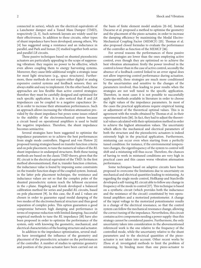
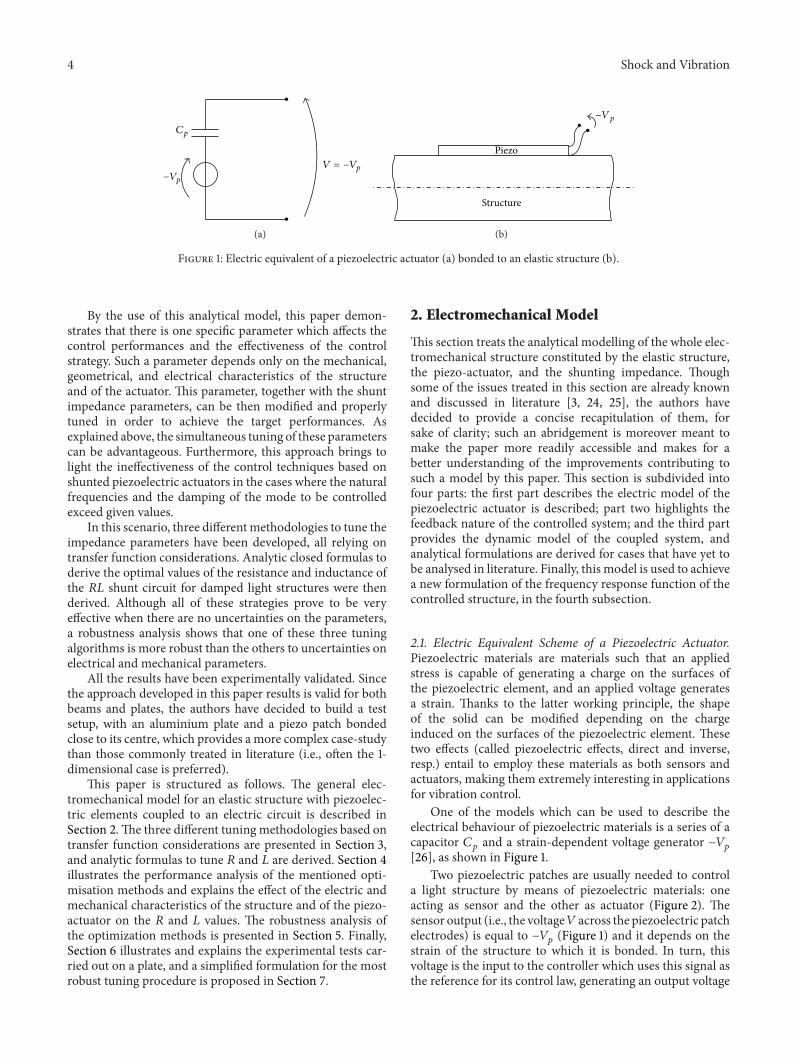
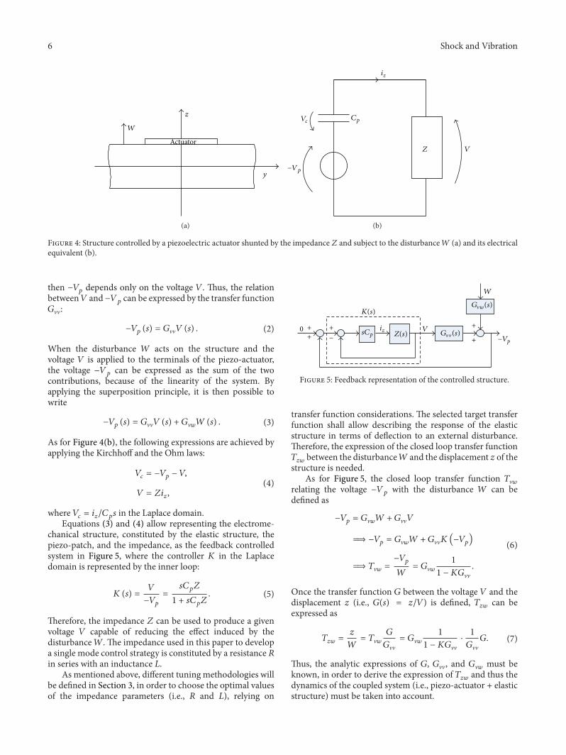
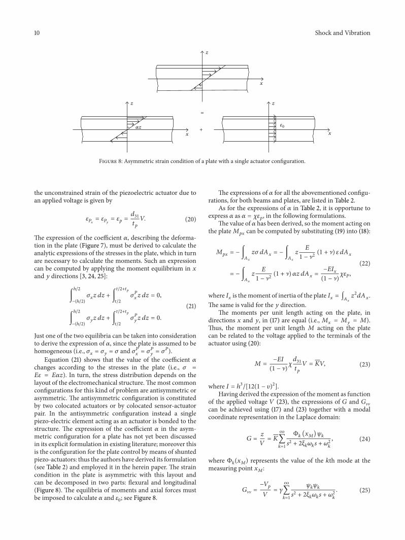
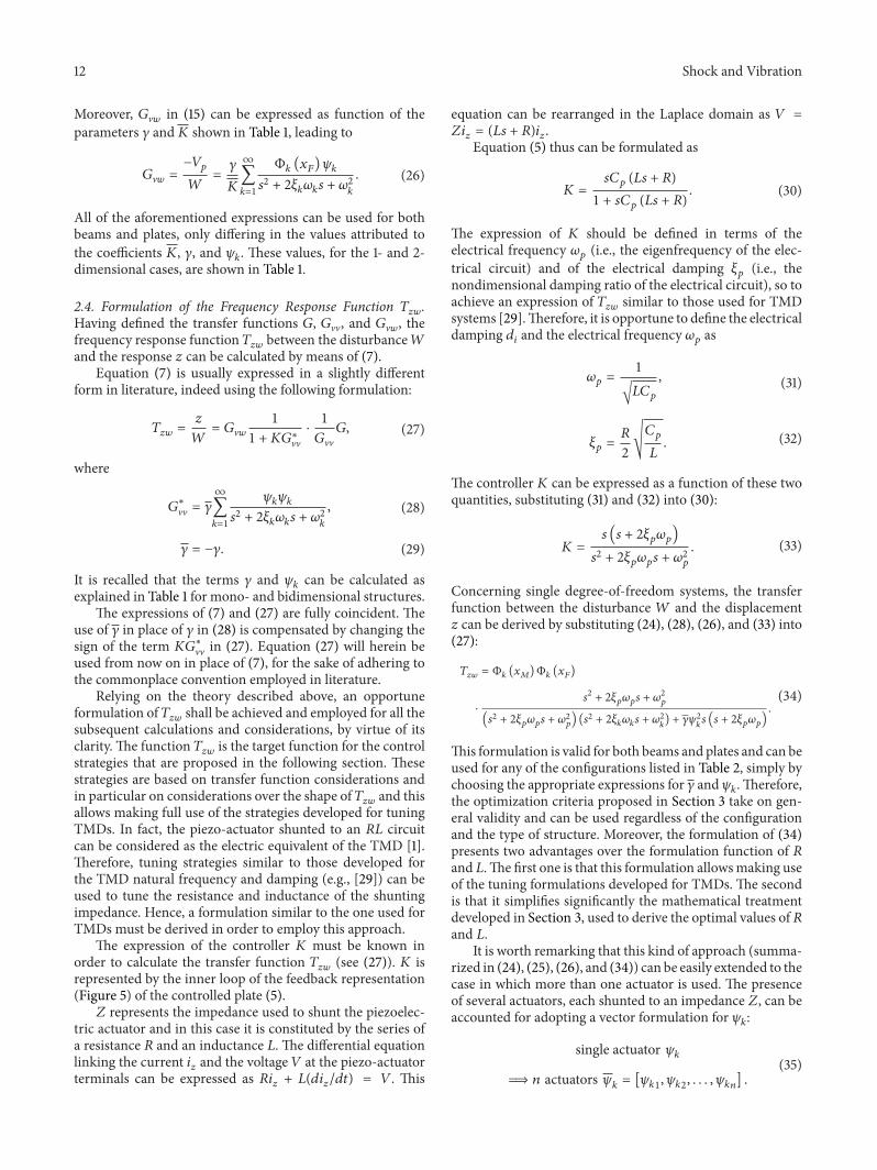
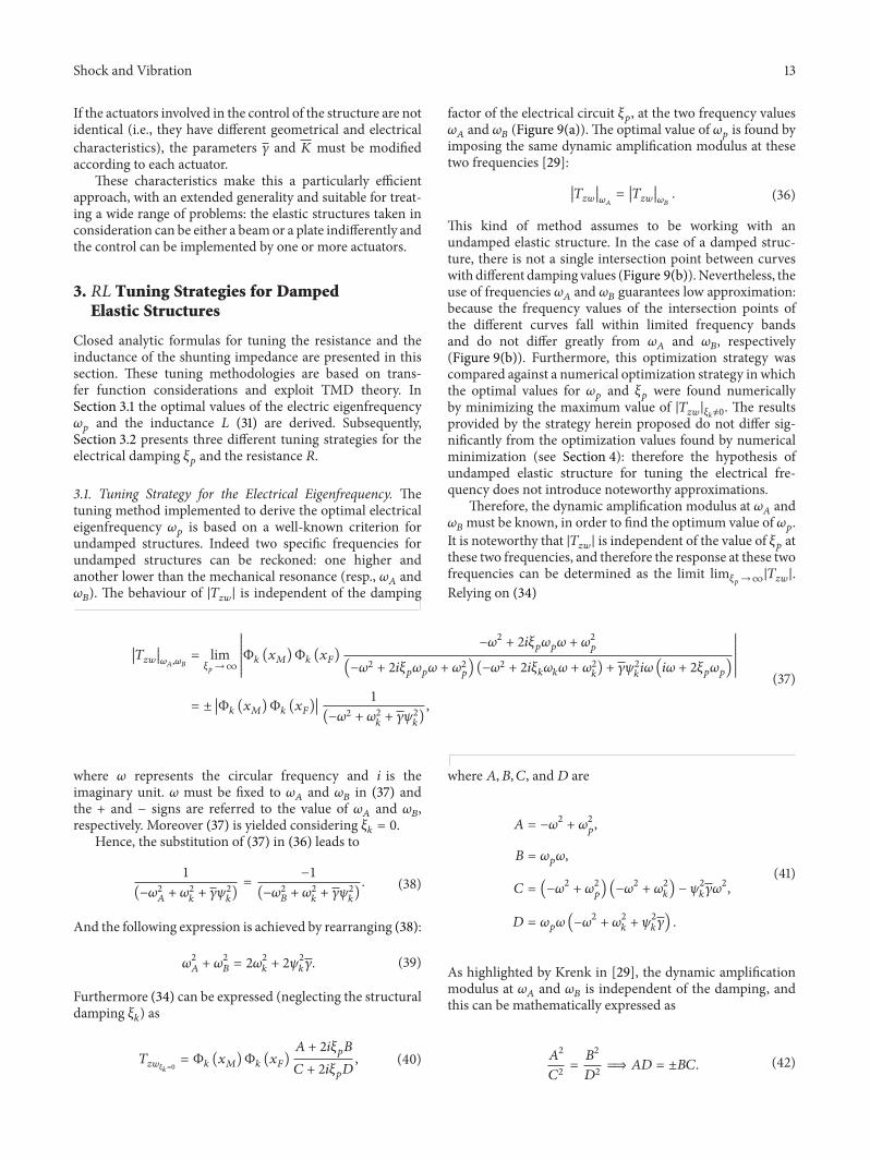
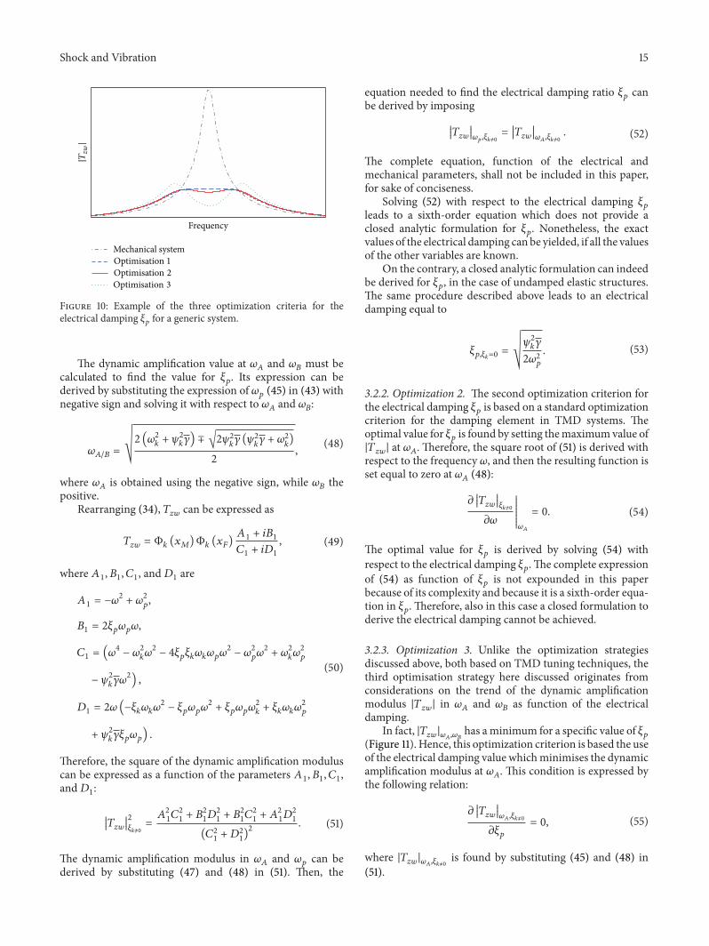
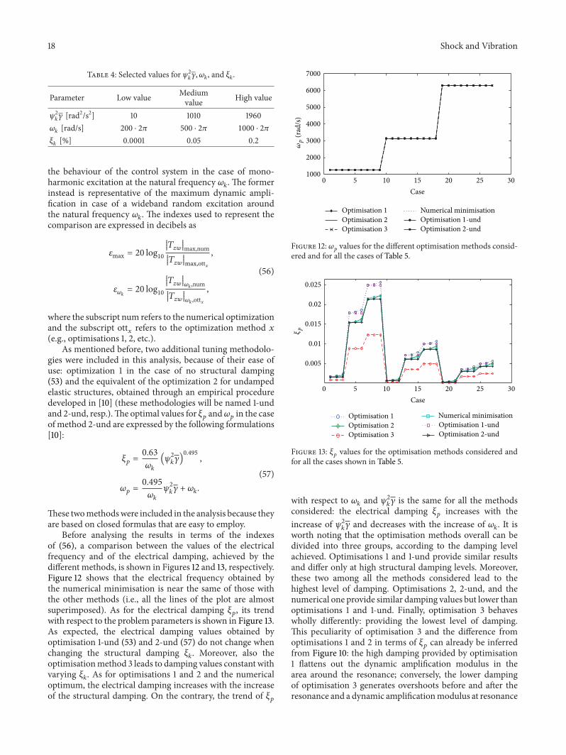
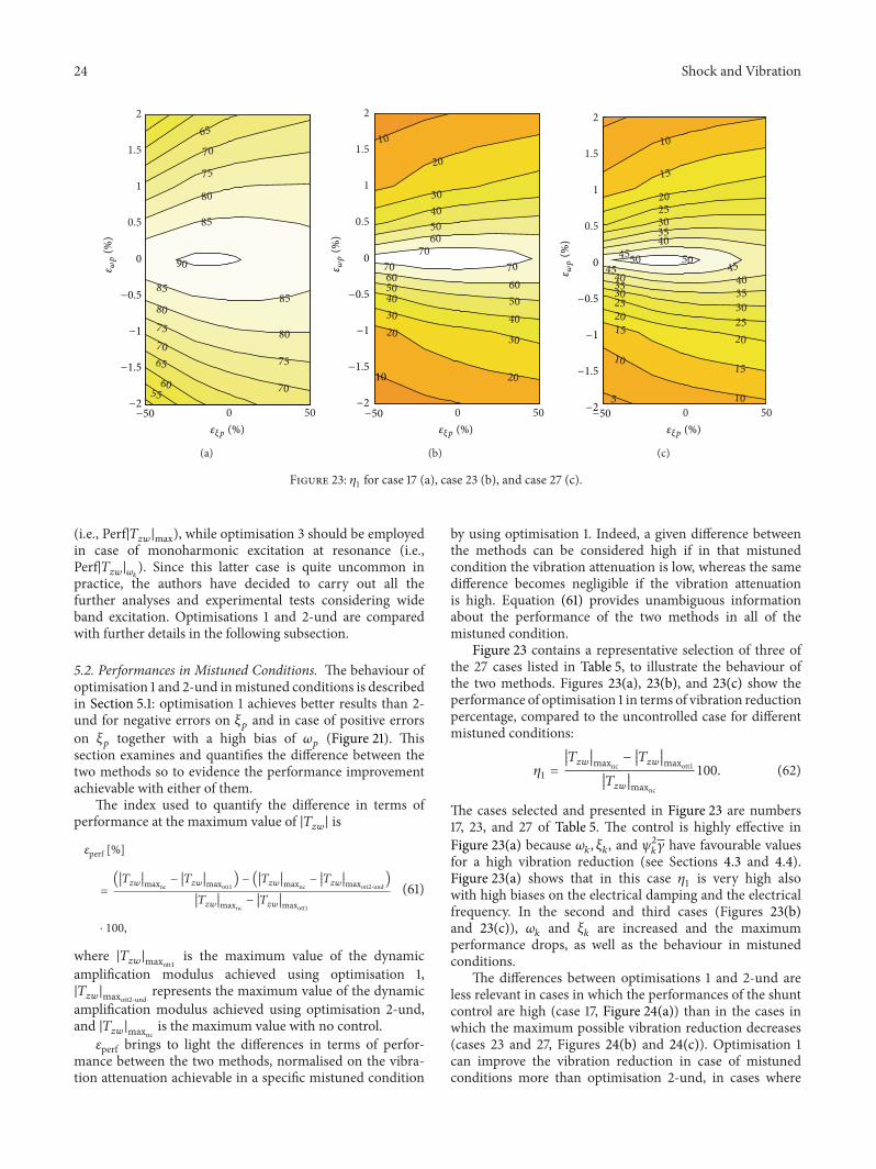
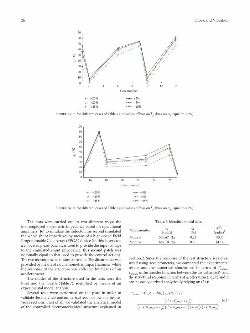
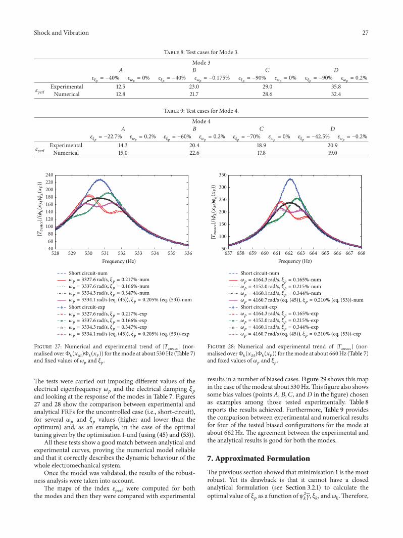
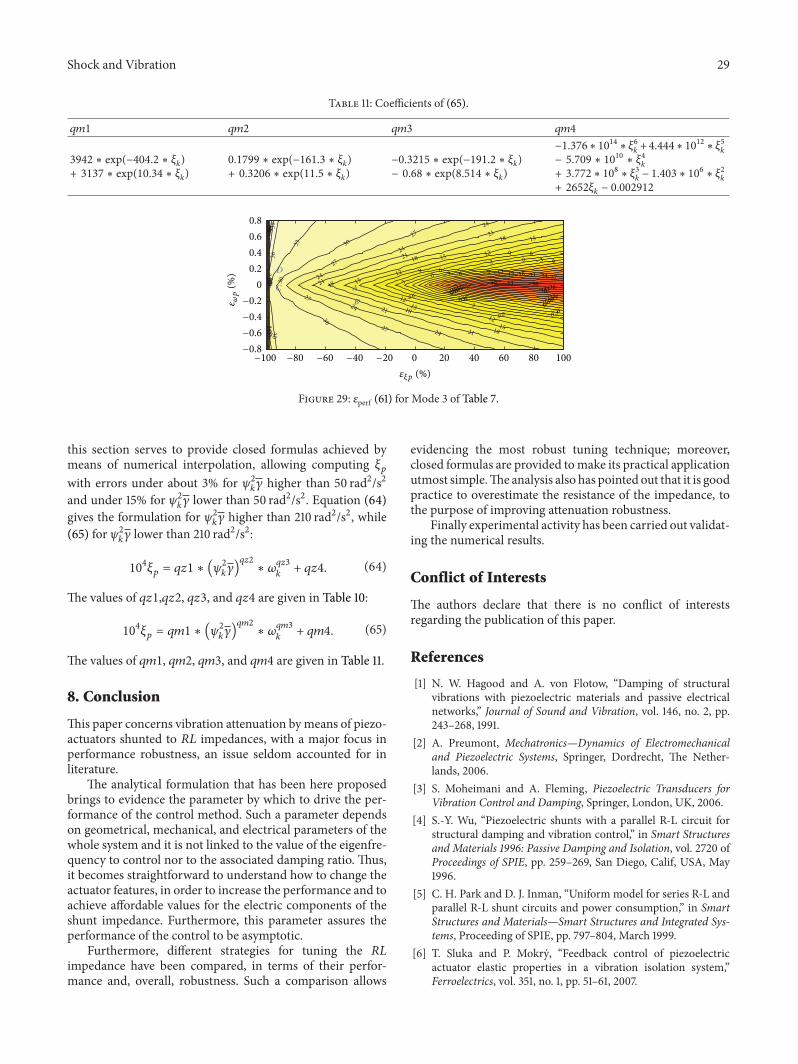

International Journal of
AerospaceEngineeringHindawi Publishing Corporationhttpwwwhindawicom Volume 2014
RoboticsJournal of
Hindawi Publishing Corporationhttpwwwhindawicom Volume 2014
Hindawi Publishing Corporationhttpwwwhindawicom Volume 2014
Active and Passive Electronic Components
Control Scienceand Engineering
Journal of
Hindawi Publishing Corporationhttpwwwhindawicom Volume 2014
International Journal of
RotatingMachinery
Hindawi Publishing Corporationhttpwwwhindawicom Volume 2014
Hindawi Publishing Corporation httpwwwhindawicom
Journal ofEngineeringVolume 2014
Submit your manuscripts athttpwwwhindawicom
VLSI Design
Hindawi Publishing Corporationhttpwwwhindawicom Volume 2014
Hindawi Publishing Corporationhttpwwwhindawicom Volume 2014
Shock and Vibration
Hindawi Publishing Corporationhttpwwwhindawicom Volume 2014
Civil EngineeringAdvances in
Acoustics and VibrationAdvances in
Hindawi Publishing Corporationhttpwwwhindawicom Volume 2014
Hindawi Publishing Corporationhttpwwwhindawicom Volume 2014
Electrical and Computer Engineering
Journal of
Advances inOptoElectronics
Hindawi Publishing Corporation httpwwwhindawicom
Volume 2014
The Scientific World JournalHindawi Publishing Corporation httpwwwhindawicom Volume 2014
SensorsJournal of
Hindawi Publishing Corporationhttpwwwhindawicom Volume 2014
Modelling amp Simulation in EngineeringHindawi Publishing Corporation httpwwwhindawicom Volume 2014
Hindawi Publishing Corporationhttpwwwhindawicom Volume 2014
Chemical EngineeringInternational Journal of Antennas and
Propagation
International Journal of
Hindawi Publishing Corporationhttpwwwhindawicom Volume 2014
Hindawi Publishing Corporationhttpwwwhindawicom Volume 2014
Navigation and Observation
International Journal of
Hindawi Publishing Corporationhttpwwwhindawicom Volume 2014
DistributedSensor Networks
International Journal of