UC IrvineUC Irvine Electronic Theses and Dissertations

TitleSimulation Studies on Dilemma Zone and Asymptotic Traffic Patterns in a Signalized Ring Road based on the Optimal Velocity Model

Permalinkhttps://escholarship.org/uc/item/212688nm

AuthorKwan, Candy

Publication Date2015

Copyright InformationThis work is made available under the terms of a Creative Commons Attribution License, availalbe at https://creativecommons.org/licenses/by/4.0/ Peer reviewed|Thesis/dissertation

eScholarship.org Powered by the California Digital LibraryUniversity of California

UNIVERSITY OF CALIFORNIA,

IRVINE

Simulation Studies on Dilemma Zone and Asymptotic Traffic Patterns in a Signalized Ring Road

based on the Optimal Velocity Model

THESIS

submitted in partial satisfaction of the requirements for the degree of

MASTER OF SCIENCE

in Civil Engineering

by

Candy Kwan

Thesis Committee:

Professor Wen-long Jin

Dr. R. Jayakrishnan

Professor Michael McNally

2015

© 2015 Candy Kwan

ii

Table of Contents Page

List of Figures ................................................................................................................................. iv

Acknowledgements ......................................................................................................................... v

Abstract of the Thesis ..................................................................................................................... vi

Chapter 1 Introduction ..................................................................................................................... 1  

Chapter 2 Literature Review ........................................................................................................... 3  

Chapter 2.1 Dilemma Zone .......................................................................................................... 3  

Chapter 2.2 Optimal Velocity Car-following Model ................................................................... 5  

Chapter 3 Computational Environment: MATLAB and CodeSkulptor .......................................... 7  

Chapter 4 Ring road with no Traffic signal ................................................................................... 11  

Chapter 4.1 Equations ................................................................................................................ 11  

Chapter 4.2 Labeling .................................................................................................................. 12  

Chapter 4.3 Implementation ....................................................................................................... 14  

Chapter 4.4 Result ...................................................................................................................... 15  

Chapter 5 Ring road with Pre-timed Signal .................................................................................. 17  

Chapter 5.1 Equations ................................................................................................................ 17  

Chapter 5.2 Implementations ..................................................................................................... 18  

Chapter 5.3 Observations and Potential Applications ................................................................ 23  

Chapter 5.4 Result ...................................................................................................................... 26  

Chapter 6 Conclusion and Future Work ........................................................................................ 34  

Chapter 7 Bibliography ................................................................................................................. 36  

Chapter 8 Appendix ....................................................................................................................... 38  

iii

Chapter 8.1 Programming Codes in MATLAB ......................................................................... 38  

Chapter 8.1a Snippets of OV Model Function ....................................................................... 38  

Chapter 8.1b Snippets of Car Spawner Function .................................................................... 38  

Chapter 8.1c Snippets of Car Update Function ...................................................................... 38  

Chapter 8.1d Snippets of Find Beacon Vehicle Function ....................................................... 39  

Chapter 8.1e Snippets of Pre-timed Signal Function .............................................................. 39  

Chapter 8.2 Programming Codes in CodeSkulptor .................................................................... 41  

iv

List of Figures Page

Figure 1. CodeSkulptor Window ..................................................................................................... 8  

Figure 2. CodeSkulptor Frame ........................................................................................................ 9  

Figure 3. Labeling of the Vehicles in the OV Model Simulation ................................................. 13  

Figure 4. Locational trajectory of each vehicle for 30 seconds (with no traffic signal) ................ 16  

Figure 5. Speed diagram of each vehicle for 30 seconds (with no traffic signal) ......................... 16  

Figure 6. Flow Chart of the Overall OV Model Simulation .......................................................... 20  

Figure 7. Flow Chart of the Determination of the Signal Timing Interchange ............................. 21  

Figure 8. Flow Chart of the Determination of the Beacon Vehicle ............................................... 22  

Figure 9. Flow Chart of the Determination of the Clearance ........................................................ 23  

Figure 10. Locational trajectory of 7 vehicles for 60 seconds (with pre-timed signal) ................. 26  

Figure 11. Speed diagram of 7 vehicles for 60 seconds (with pre-timed signal) .......................... 27  

Figure 12. Locational trajectory of 7 vehicles for 300 seconds (with pre-timed signal) ............... 28  

Figure 13. Speed diagram of 7 vehicles for 300 seconds (with pre-timed signal) ........................ 28  

Figure 14. Locational trajectory of 10 vehicles for 300 seconds (with pre-timed signal) ............. 29  

Figure 15. Speed diagram of 10 vehicles for 300 seconds (with pre-timed signal) ...................... 29  

Figure 16. Locational trajectory of 15 vehicles for 300 seconds (with pre-timed signal) ............. 30  

Figure 17. Speed diagram of 15 vehicles for 300 seconds (with pre-timed signal) ...................... 30  

Figure 18. Percentage of Stopping Time for 3 hours (where there are 7 vehicles) ....................... 31  

Figure 19. Percentage of Stopping Time for 5 hours (when there are 10 vehicles) ...................... 32  

Figure 20. Percentage of Stopping Time for 12 hours (when there are 15 vehicles) .................... 33  

v

ACKNOWLEDGMENTS

I would like to express the deepest appreciation to my committee chair, Professor Wen-long Jin,

who first invited me to do research with him since my undergraduate study and continuously

supports me even until now in my graduate study.

I would also like to express my gratitude to my committee members, Dr. R. Jayakrishnan and

Professor Michael McNally, for accepting my invitation to be a part of my thesis committee and

always being responsive to my questions and concerns.

In addition, I offer my sincere appreciation for all the learning opportunities provided by the

professors, teaching assistants, and staffs throughout the graduate program.

Further, I have to thank all my colleagues and friends who have supported me on the completion

of this thesis.

Lastly, I would like to thank University of California Transportation Center (UCTC) and the

Institute of Transportation Studies at the University of California, Irvine for providing funding

support for the graduate program.

vi

ABSTRACT OF THE THESIS

Simulation Studies on Dilemma Zone and Asymptotic Traffic Patterns in a Signalized Ring Road

based on the Optimal Velocity Model

By

Candy Kwan

Master of Science in Civil Engineering

University of California, Irvine, 2015

Professor Wen-long Jin, Assistant Professor

While traffic light is used to coordinate vehicular and pedestrian traffics in order to

provide safety to drivers on streets, there are delays and accidents resulted from unorganized

signal timing and poor network design. At every signalized intersection at the yellow light onset,

drivers have to make an uncertain decision in an area called the dilemma zone. It is where the

drivers have to decide whether he can stop safely by the stop line or clearly proceed through the

intersection. Because of the potential safety issues from the dilemma zone, this thesis attempts to

simulate traffic flow in a single-lane ring road with and without the presence of a traffic signal

by using the Optimal Velocity (OV) car-following model. In particular, a beacon vehicle is

selected as the first vehicle to stop, and all following vehicles have to stop accordingly. Using

programs such as MATLAB and CodeSkulptor, the simulation demonstrates the leading and

following vehicles’ behavior with location and speed trajectory diagrams and it is found that the

OV model produces a collision-free scenario even under the presence of a traffic signal. In

addition, by observing a single vehicle’s behavior, some asymptotic traffic patterns can be seen.

This thesis can serve as a fundamental study to inspire and develop potential dilemma zone

protection to promote intersection safety and prevent risks such as rear-end accidents and red

light violations.

1

Chapter 1 Introduction

In the road traffic network, signalized intersections pose safety and mobility issues to the

drivers. While traffic signals are used to coordinate road traffics and to allow for the shared use

of road space with pedestrians, cyclists and vehicles, congestion and accidents typically occur at

signalized intersections. According to the Signalized Intersection Information Guide (2013) [1],

21% of all the crashes and 24% of all fatalities and injuries collisions occurred at signalized

intersections in the year of 2009. The problem in question is that the drivers do not know

whether they should proceed or stop when they see the light changes to yellow. The road length

that the drivers are in when they have to make such a decision is called a dilemma zone. It is

where the drivers are either being too close to the stop line to stop safely or too far from the

intersection to pass through it entirely at the onset of the yellow light. Because of such a

conflicting decision, potential risks such as rear-end accidents and red light violations can occur,

which is why the study of dilemma zone is very important in finding the protection from it.

The most common dilemma zone protection that some States use is the 5 seconds rule of

thumb [1] and the extension of the yellow interval. It provides a safe distance to some extent, but

depending on the traveling speed and acceleration, drivers may still have conflicting decisions as

to whether to stop or proceed. Since they do not know the length of the yellow light and lack the

understanding of the yellow light interchange, this may increase the potential risk of a rear-end

accident and red-light violation. While there are many factors that affect the safety at a signalized

intersection: human behaviors, geometric design, traffic design and control, understanding how

vehicles behave in the dilemma zone and their traffic patterns can help future studies and identify

the problems that traffic engineers should look into in order to balance the safety and mobility of

the drivers at signalized intersections.

2

This thesis will focus primarily on the traffic signal timing as well as how the drivers

approach an intersection. Simulation studies have been conducted in order to observe the effect

of dilemma zone and the traffic patterns in a microscopic level. Even though the parameters are

predefined by designed values from various studies and reports, the Optimal Velocity (OV) car-

following model will be used to represent each individual vehicle’s behavior, by updating the

acceleration, velocity and trajectory with time. In particular, this thesis will model vehicles’

behaviors at the onset of yellow and draw observations from it.

Beginning with the reviews of earlier research about the yellow light dilemma zone and

the OV car following model, this thesis will then provide a basic introduction of the

programming environments that were used for simulation. Then, the traffic flow simulation in a

ring road with and without traffic signals will be explained from the equations and

implementations, to the results. This thesis will then close with a conclusion and includes some

discussions of the future work.

3

Chapter 2 Literature Review

Chapter 2.1 Dilemma Zone

According to the Traffic Signal Timing Manual (2008) [2], the intent of the yellow light

change is to provide a safe transition to the red light from the green light. However, it creates a

fuzzy meaning to the drivers that they will find themselves in what is called the dilemma zone.

Gazis et al. (1960) [3] first introduced the concept of dilemma zone by analytical consideration

and real-life observation when they examined the problem of the yellow light in traffic flow.

They discussed that the dilemma zone is the area when drivers have to decide whether to stop or

to proceed through the signalized intersection at the onset of yellow light. Their study identified

the complexity and made others aware of the problem of the yellow light interval. This

eventually inspired many researchers to further study the effects of the dilemma zone and to

propose protection that can eliminate the conflict from it.

One of the effect of the dilemma zone is the increased risk of the occurrence of rear-end

accidents. Rear-end accidents are one of the most common types of accidents that happened at a

signalized intersection because of the abrupt stop that the driver makes at the stop line due to the

decision that the driver has to make in the dilemma zone. Yan, Radwan and Abdel-Aty (2005)

[4] used binary logistic regression models to identify factors that are related to rear-end crashes

at signalized intersections. They found that road environment factors such as the number of

lanes, divided/undivided highway, accident time, road surface condition, highway character,

urban/rural, and speed limit, are significantly associated with the risk of rear-end accidents.

Especially due to the approach speed limit at the intersection, they found that drivers are more

likely to fall into the dilemma zone with the decision of whether they can cross the intersection

completely or to stop comfortably at the yellow light onset.

4

Because of the uncertain decision in the dilemma zone, red light running violation is also

a major effect due to the dilemma zone. Using a video-based system, Elmitiny et al. (2010) [5]

associated drivers’ stop or go decision and red light running violation with the vehicle’s yellow-

onset distance, operating speed, and position in the traffic flow. The study suggests that lowering

the drivers’ approaching speed to the intersection may reduce the possibility of red light running

violations. However, Elmitiny et al. found that the following vehicles are more likely to make go

decisions and run the red light than the leading vehicles. This means that rear-end accidents are

more probable and is actually similar to what other research papers have observed. It can be seen

that many researches agreed that the dilemma zone is the primary cause to the danger of

signalized intersection, which leads to other researchers to propose yellow light settings that can

eliminate the conflict from the dilemma zone.

In order to eliminate the dilemma zone at the onset of yellow light and to reduce incidents

such as the rear-end crashes and red light violations, Zimmerman et al. (2004) [6] suggested that

the number of vehicles in the dilemma zone indicates the frequency that drivers are forced to

make an uncertain decision of whether to go or to stop at the end of a green traffic light, which

partly causes the many crashes at intersections. They believed that the number of vehicles in the

dilemma zone could be used as a potential intersection safety measure and reducing it can reduce

the safety risks that occur at a signalized intersection. Bonneson et al. (2004) [7] studied the

before-and-after effect of increasing the yellow light interval and they actually found that even if

the drivers adapted to the change, there is still a benefit of reducing the safety risks. In support to

this, Liu et al. (1996) [8] actually reexamined the dilemma zone using the methodology given by

Gazis et al. in 1960 and suggested a possible solution to eliminate it. By knowing the speed

distribution function of the approaching vehicles, it is possible to compute the required yellow

5

timing for them to clear the intersection. As observed from this thesis, knowing the initial speed

and the acceleration of the vehicles can also be used to compute the yellow timing. By changing

the yellow light duration, it can allow for all the approaching vehicles to clear the intersection.

However, some studies have opposing view toward the extension of the yellow light and

believe that changing the yellow light timing alone will not be satisfactory. Liu, Chang, Tao,

Hicks, and Tabacek [9] suggested in a 2007 study that it is necessary to have a vehicle detection

module and a signal control module in order to minimize the safety issues caused by the different

dilemma zones from various intersections. Their proposed modules will acquire the vehicle’s

speed and position information to analyze whether the vehicle is within the dilemma zone. Then,

the signal control module will react accordingly, such as to extend the red clearance time, for the

safety of the vehicles. Zimmerman et al. (2012) [10] conducted a more detailed study on a

vehicle-specific detection, control, and warning system a few years later. The system reduces the

number of vehicles trapped in the dilemma zone by controlling the signal phases and warning the

drivers ahead of them that they should probably stop. However, while all of these modern

technologies proposed to increase the safety at a signalized intersection are explored, their

practical usage in the real-time traffic network is still under study due to the complexities of the

dilemma zone.

Chapter 2.2 Optimal Velocity Car-following Model

As many studies about the yellow light dilemma zone mentioned, knowing the speed and

the acceleration of the vehicles will be useful for traffic detection and beneficial to calculate the

yellow signal time duration for the safety in the intersection. In this thesis, in order to reproduce

real-time traffics on the single-lane ring road simulation, the speed and acceleration are

controlled using the Optimal Velocity (OV) car-following model.

6

Bando et al. (1994, 1995, 1998) [11, 12, 13] proposed the OV model as follows:

𝑎!!"(𝑡) =  1𝑇   min 𝑉,

1𝜏 𝑥!!!(𝑡)− 𝑥!(𝑡)− 𝑆! −  𝑣!(𝑡)   (1)

Where,

n stands for the index of the vehicle,

n – 1 is the vehicle that precedes the n-th car,

T is the reaction time in seconds (which is 1.2 seconds),

τ is the time gap in seconds (which is 1.6 seconds),

V is the free flow speed in feet per seconds (which is 65 ft/s),

Sj is the jam spacing in feet,

𝑥!!!(𝑡)− 𝑥!(𝑡)− 𝑆! is the clearance.

It describes that if there are no leading vehicles, the vehicle will travel at the free flow

speed as fast as the driver wants. However, if there is a leading vehicle, the vehicle’s optimal

velocity depends on the distance from this preceding vehicle that the driver wants to keep. In this

case, the safe distance is at least a car length apart. In addition, the acceleration will depend on

the difference between the current vehicle’s velocity and the optimal velocity, as well as taking

into account of the reaction time of the driver. This will be the default car-following model used

in the simulation.

7

Chapter 3 Computational Environment: MATLAB and CodeSkulptor

There are two computational environments that are utilized in this thesis. The primary

one is called MATLAB and the supportive one is called the CodeSkulptor. Because MATLAB is

more widely known compared to CodeSkulptor, this chapter will tend to explain CodeSkulptor in

greater depth than MATLAB.

In this thesis, MATLAB is primarily used for data analysis. It is a computing language

environment that is good for algorithm development and data visualization that this thesis

heavily depends on. It supports feature from traditional programming languages and can produce

results immediately by executing the commands. It is also relatively simple to draw charts and

graphs resulted from the traffic flow simulation; thus, it is particularly chosen for the scope of

this thesis.

CodeSkulptor [14] is a browser-based Python programming environment that runs with

full functionality in Google Chrome, Mozilla Firefox, and Apple Safari. Its window consists of

the control area in the upper left, useful resources in the upper right, program editor for typing in

Python codes in the left, and the console is on the right. The control area consists of buttons that

allow the users to run the program, save, download, create fresh URL, open local file and reset.

When the program is first saved, a URL link is generated so the users can access their codes on

the specified browsers. Then as the program is modified and updated, saving it will generate a

new version of the URL link, such as adding to the end of the URL the version number, without

overwriting the old version so that the users can refer back to the previous URLs at all times.

Figure 1 shows the typical start up window of CodeSkulptor.

8

Figure 1. CodeSkulptor Window As you can see from Figure 1, there is already a sample program written on the editor and

the code is color coded, allowing users to easily differentiate between the usages of words. For

example, numbers, such as integer, float, double, are in green; strings, usually in single or double

quotations, are in red; predefined words, such as if, def, import, are in violet; and comments,

those lines starting with the number sign (#), are in brown.

9

Figure 2. CodeSkulptor Frame

Once the editor with the color codes is ran, the window shown in Figure 2 will pop up.

This window is called a frame. Of course, a program does not need to have a frame to pop up if it

is not the necessary outcome, but a program can create only one frame. A frame starts when the

users call on the start() method after specifying the attributes required to create a frame. The

frame contains the canvas, controls, and status information that help the users visualize their

results. The canvas, which is the black rectangular background on the right in Figure 2, can be

size-adjusted. It is necessary to have the canvas to illustrate what the users want to show by using

the draw(canvas) method. Such a method is typically called a handler because it handles what the

canvas draws and the handler can also be applied to the controls. The control, which in this case

is the button Click me, can be buttons, inputs, or labels that the users want to interact with the

program. Once a certain control is activated, the handlers will handle the reaction of that

activation and produce results accordingly. And finally, the status information, which are the two

boxes on the bottom that starts with Key: and Mouse:, tells the users which key is being used and

10

whether there are mouse clicks. These information and attributes in a frame help the users to

communicate and visualize the results.

While it is great that CodeSkulptor can be used to generate illustrations of the simulation,

it is quite difficult to analyze the results from the simulation because there are no simple method

to store all the necessary traffic flow data for graphs and charts, other than to use programs like

Excel. Because of such redundant maneuver, CodeSkulptor is only utilized in the first scenario of

the thesis and serves as a crosscheck and provides visualization to the result from MATLAB. In

the following chapters, the findings and implementation of the ring road simulation with and

without traffic signal using MATLAB as well as CodeSkulptor will be explained, along with the

formulas and methods that are involved.

11

Chapter 4 Ring road with no Traffic signal

In order to get the fundamentals of the OV model, the simplest road network is one when

there is no traffic signal on a single lane ring road. There are also no communications between

the vehicles nor can the following vehicle pass the leading vehicles. This will serve as the

foundation of the next implementation where a traffic signal will be installed.

Chapter 4.1 Equations

While the simulation uses the default OV model in Equation 1, three modifications are

included to the resulting acceleration on the vehicles:

1) Bounded acceleration

𝑎!!(𝑡) = max 𝑎!"#,min 𝑎!"# ,𝑎!!"(𝑡) (2)

2) Collision free

𝑆! =   2   𝑥!!!(𝑡)−  𝑥!(𝑡)−  𝑆! 𝑎

(3)

𝑎!!(𝑡) = 𝑚𝑖𝑛2∆𝑡!   𝑥!!! 𝑡 − 𝑥! 𝑡 − 𝑆! −  𝑣!(𝑡)∆𝑡

−  12  𝑎  (∆𝑡 −  𝑆!)

! ,𝑎!!(𝑡)

(4)

3) No negative speed

𝑎!!(𝑡) = max   −

𝑣! 𝑡∆𝑡 ,𝑎!!(𝑡)

(5)

Bounded acceleration restricts the maximum and minimum acceleration rate that a

vehicle can have. The values are generally 9.8425 ft/s2 for acceleration and 13.1234 ft/s2 for

deceleration. Collision-free is a modification that prevents vehicles from crashing into each

12

other. However, to simplify the equations and to have the absolute collision-free situation,

bounded deceleration is removed. Finally, there can be no negative speed for any vehicles,

meaning that the vehicles will not travel backward. These modifications will allow for more

realistic simulations that can better represent the road traffics. However, they are necessary to be

implemented in sequential order to prevent any computation errors.

In order to update the velocity and position of the vehicles, the following formulas are

used:

𝑣! 𝑡 +  ∆𝑡 = 𝑣! 𝑡 + 𝑎!! 𝑡 ∙ ∆𝑡 (6)

𝑥! 𝑡 +  ∆𝑡 =  𝑥! 𝑡 + 𝑣! 𝑡 ∙ ∆𝑡 +12𝑎!

! 𝑡 ∙ ∆𝑡! (7)

Or, the position update can also use the following equation:

𝑥! 𝑡 +  ∆𝑡 =  𝑥! 𝑡 +  𝑣!(𝑡 +  ∆𝑡) ∙ ∆𝑡 (8)

The difference between the two position update equations, Equation 8 and Equation 7, is that

Equation 8 has to occur after the velocity is updated, as you can see that the velocity in this

formula is 𝑣! 𝑡 +  ∆𝑡 instead of 𝑣! 𝑡 . Thus, depending on the order of implementation, both of

these equations can be used but in this thesis, Equation 8 is used.

Chapter 4.2 Labeling

In CodeSkulptor, the vehicles follow a typical labeling method that is also referred to

when imagining this ring road with MATLAB. The vehicles are indexed in order

counterclockwise against the direction of travel on the ring road. The vehicle in the front always

has a smaller index number except for the first vehicle, which is why when implementing, it

13

requires a special case to handle this exception. Figure 3 shows an example of the start up screen

for the simulation with the labeling on the vehicles as well as the traveling direction. The defined

ring road is one single lane with a specified length of 5000 ft and a free flow velocity of 65 ft/s.

The vehicles also have defined characteristics such as maximum and minimum acceleration,

maximum and minimum starting velocity, and jam spacing and they are initially generated with

equal distance apart. The simulation does not allow any vehicles to enter or leave the ring road

and there is also no overtaking or parking allowed during the simulation.

Figure 3. Labeling of the Vehicles in the OV Model Simulation

14

Chapter 4.3 Implementation

The implementation of the OV model simulation is relatively simple on MATLAB. The

first function to be implemented is the OV model with modifications. It contains the default

equation of the OV model (Equation 1) and the additional equations (Equations 2-5) for

modifications, with transformation to change them into the functions of the MATLAB language.

These functions are shown in the Appendix. Then, a function to spawn the vehicles is created in

a separate document to keep the codes in a neat format. This function only serves to spawn the

number of vehicles in the ring road in equal distance away from each other. Of course, it can be

randomized to better represent the real-time traffic, but this thesis only hopes to start in a simple

scenario; thus, the vehicles are initialized with the equal distance apart. However, the vehicles

have initial speeds that are randomly ranged from 22 ft/s to 65 ft/s in order to observe how the

various starting speeds will affect their trajectory. Finally, the main algorithm of the

implementation is to update the vehicles and to plot the results. While it calls for the OV model

and the vehicle spawn function, it basically contains a for-loop to update the location, velocity

and acceleration of each vehicle by using the motion equations as shown in Equations 6-8.

Similar logic is used in the CodeSkulptor implementation, but the functions that are in the

MATLAB will become the methods within the class. The Car class contains three methods:

initiation, draw, and update. In the initiation method, a car is defined to have six attributes. It has

an index that is used to identify the car, position that specifies the center of the image that is to

be drawn on canvas, location that shows where the car is located on the ring road, velocity,

acceleration, and image of the car that is used to show up on the canvas. In the draw method, it

draws the image and the index whenever it is called. Then in the update method, the car will be

updated in its location, its velocity, and position. With the Car class implemented, a

15

car_spawner method is built outside of the class that is used to spawn car(s) at the start of the

simulation. This method will give all the vehicles their attributes that are defined by the user, and

it is noted that each vehicle’s velocity is randomly selected between the vehicle’s maximum and

minimum starting velocity. Finally, the main logic of the simulation is on the car_update

method, which determines the acceleration that will be used in the update method in the Car

class. This method calls the OV calculation that follows the logic of the OV model and the three

modifications to determine the acceleration. It is important to notice though, that for the first

vehicle, the clearance will have to add the ring road length in order to avoid computational

errors. After the logic of a car-following model is implemented, the user can start the simulation

by clicking the start button. The simulation time will begin counting and the vehicles, total of 7

vehicles but can be modified to observe other congestion levels, will follow the OV model as

they travel on the ring road of 5000 feet long. The programming codes of the implementation in

both of these environments are shown in the Appendix.

Chapter 4.4  Result

The vehicles follow the modified OV car-following model as they travel along the ring

road with no traffic signal. The speed as well as the trajectory for each vehicle can be printed to

the console. However, because there is not a function for writing data to file in CodeSkulptor, the

data will be processed and graphed using Excel. Because the printed result in the console is raw,

an OFFSET function is used in Excel to organize the data, which will then be used to graph. The

same diagrams can also be observed using MATLAB, which shows the validity of the

implementation of the formulas in both environment. From Figure 4, the trajectory of each

vehicle is shown and one can notice that the vehicles do not crash into one another and that they

are moving in a constant slope. However, it is observable that the speed varies drastically. In

16

Figure 5, the instability of the vehicles is shown and eventually, they maintain a constant

distance at the free flow speed. The implementation from this chapter can be used as the

underlying structure for the later chapter.

Figure 4. Locational trajectory of each vehicle for 30 seconds (with no traffic signal)

Figure 5. Speed diagram of each vehicle for 30 seconds (with no traffic signal)

17

Chapter 5 Ring road with Pre-timed Signal

The next scenario to be looked at is a signalized ring road. This can be visualized as an

infinite long road that has synchronized traffic signals. A traffic signal is installed in order to

provide safe accessibility to the drivers. According to the Traffic Signal Timing Manual [2],

there are two types of traffic signal operation: pre-timed and actuated mode. The pre-timed

operation controls the timing of the light with a fixed duration. It means that the signal does not

change according to any real-time traffic condition but has a predefined time set on each green,

yellow, and red light. This pre-timed set can be changed according to the time of day, such as

when it is peak hour, but does not depend on the current road traffic. It is predictable and of

lowest cost of equipment and maintenance. On the other hand, actuated operation controls the

timing based on the presence, or absence, of a vehicle. It typically uses detection devices such as

loop detectors and cameras to respond to the changing traffic patterns. In this thesis, only the pre-

timed operation will be looked at because of its fundamentality and simplicity, but in the future,

the study on actuated controls will also be considered.

Chapter 5.1 Equations

In addition to the equations from the scenario of a ring road with no signal, a pre-timed

signal will make a vehicle to stop when the light is red, thus a stopping distance is to be

calculated as follows,

𝐷!"#$%&' =  

𝑣!

2𝜇𝑔 (9)

Where,

𝑣 is the initial driving speed (ft/s),

µ is the coefficient of friction between the road and the tires (which is 0.7), and

18

g is the gravity of Earth (which is 32.17 ft/s2).

Or in another form,

𝐷!"#$%&' =

𝑣!

2𝑎 (10)

Where 𝑎 is the acceleration of the vehicle (ft/s2).

However, because there is a reaction time for the driver, another distance is added which

result in the total stopping distance to be as follows,

𝐷!"!#$ = 𝐷!"#$%&'( + 𝐷!"#$%&' = 𝑣𝑡!"#$%&'( +

𝑣!

2𝜇𝑔 (11)

Based on a common value, the reaction time is approximately 1.2 seconds and the

coefficient of friction is to be 0.7.

Chapter 5.2 Implementations

The implementation of this signalized ring road is built upon the implementation without

the traffic signal in the previous chapter. In the process of implementing this ring road with pre-

timed traffic signal, flowcharts are made in order to better understand the concepts and the scope

of the implementation. In Figure 6, the overall process that the implementation involves is

produced. First, the initialization process begins at time zero. Each vehicle’s location is

initialized with equal distance apart based on the car spawning method, the beacon vehicle index

is none, and that the indicator for the current signal (signal_now) is green (G) but the previous

signal (signal_bef) is red (R). After the initial conditions are set up, two decisions have to be

made before the process continues. Both of the decisions involve checking the signal_bef and

signal_now indicator. The process for implementing this is shown in Figure 7. The initial stage is

basically the same as the initialization process from the overall flowchart. In order to determine

19

the timing, a simple mathematical operation called the modular is used. This will capture the

time when green changes to yellow as well as when red changes to green. These will be the exact

moment when a decision is needed to proceed through the ring road. In order to update the signal

indicators, two decisions are also required in order to set the indicators correctly. This step will

occur at the end of every time step and the initial condition is the same as how the overall

flowchart has. If the time t is the remainder of green time divided by the cycle time, then

signal_bef = G and signal_now = Y; however, if the time t does not have remainder, then

signal_bef = R and signal_now = G. This will then lead to the next time step and will continue

on through the rest of the overall flowchart.

As the signal changes from green to yellow, meaning that signal_now = Y and signal_bef

= G, the next step will be to find beacon vehicle and add it to the array. The beacon vehicle is the

first vehicle, found to be unable to safely stop by the stop line that will approach the intersection

at the onset of yellow. It is selected as the first vehicle to stop, and all following vehicles have to

stop accordingly. In order to find the beacon vehicle, another flowchart is made to demonstrate

the detailed steps in this process, as shown in Figure 8. First, the vehicles are sorted based on

their distance to the stop line. The vehicle closest to the stop line should be stored first, and

continued storing in an ascending order. After the vehicles are sorted, then each vehicle’s

location is checked against its stopping distance, which can be calculated with Equations 9-11.

The first vehicle that has a location greater than the stopping distance will be the beacon vehicle.

As the signal changes from red to green, meaning that signal_now = G and signal_bef =

R, the next step will be to empty the beacon vehicle array. Either the beacon vehicle array is

empty or not, the next step will be to follow the OV model. However, if none of the signal-

changing situation occurred, the entire process will also continue with the OV model. This OV

20

model also has a flowchart, as shown in Figure 9, to determine the clearance based on the car

index as well as whether a beacon vehicle exists. If the car index is 1, the clearance will depend

on the location of the last vehicle; or if a beacon vehicle exists, the clearance will depend on the

location of the signal and the beacon vehicle. If none of these occurred, then the clearance is

based on the difference between the leading and current vehicle’s location. After this, the

acceleration will be calculated and updated. The entire process will be looped multiple times

until the simulation time is reached.

Figure 6. Flow Chart of the Overall OV Model Simulation

21

Figure 7. Flow Chart of the Determination of the Signal Timing Interchange

22

Figure 8. Flow Chart of the Determination of the Beacon Vehicle

23

Figure 9. Flow Chart of the Determination of the Clearance

Chapter 5.3 Observations and Potential Applications

After the flowcharts are created and implemented in MATLAB, intriguing observations

are made during the implementation phase that provides insights on the feasibility of Vehicle-to-

Vehicle (V2V) and Vehicle-to-Infrastructure (V2I) communications. The first observation came

to attention when the vehicles are sorted in order of the distance closest to the stop line. In order

to find the beacon vehicle, the location of the vehicle, say di, has to be compared to the stopping

24

distance, say si. For each vehicle, the stopping distance is different based on its traveling speed.

So once there is a sorted list of vehicles that are already lined up in order of the closest distance

to the stop line, then the beacon vehicle will be the first vehicle with the location that lies outside

of its stopping distance. However, even if the beacon vehicle is found, it is still possible for the

following vehicles to be in the location that is also greater than the stopping distance. This means

that the following vehicle can actually pass the intersection if the leading vehicle does not stop.

Thus, if 𝑑!  ≥   𝑠! but 𝑑!  ≤   𝑠! such that 𝑠! ≥ 𝑑! ≥ 𝑑! ≥ 𝑠!, this scenario can be imagined as to

having a vehicle in front of you that is slower than your traveling speed which forces you to stop,

though in theory, you are able to pass through the intersection without the leading vehicle. In

such case, rear-end accident could occur easily and the V2V communication would actually be

beneficial. If the vehicle knows that the leading vehicle is going at a slow speed and ready to

stop, then it is possible for the driver to slow down earlier in case of any accidents.

Another observation is made on the infrastructure side. As mentioned, the stopping

distance for each vehicle is dependent on its speed, which means that in order for each vehicle to

successfully pass the intersection, the signal timing has to be different for each vehicle in order

to accommodate this premise. This can be demonstrated in the following:

𝑣!

2𝑎 + 𝑤 + 𝐿 = 𝑣 ∙ 𝑌 (12)

Where,

𝑣 is the vehicle’s speed (ft/s),

𝑎 is the vehicle’s acceleration (ft/s2),

𝑤 is the width of road (ft),

𝐿 is the vehicle’s length (ft), and

𝑌 is the yellow light timing (s).

25

Rearranging Equation 12,

𝑌 =  𝑣2𝑎 +  

𝑤 + 𝐿𝑣 (13)

Since !!!!

is the all-red time, this will mean that the yellow timing is dependent on !!!

, the

individual vehicle’s speed and acceleration. In standard design procedures, the stopping distance

is usually calculated by the average and according to the Signalized Intersection Information

Guide [1], there is typically a chart of recommended design values of stopping distance to

follow. However, if the signal can be coordinated according to the vehicles, delay may be

reduced. This is an interesting finding that shows the potential application of the V2I

communication. If the vehicle sends the necessary information, such as its speed, acceleration

and direction, to the infrastructure, which is the traffic signal, the signal can then react

accordingly or even provide information back to the vehicle in order to reduce conflicts and

promote safety.

There are actually studies from various institutes and developments from the U.S.

Department of Transportation [15, 16] on V2I communication and V2V communication. The

communication may includes data transmission from the vehicle to the traffic light signal, such

as speed, location, route of travel, etc., or otherwise from the signal to the vehicle, such as its

timing. These data transmission is in real-time so that the vehicle and/or the infrastructure can

use the data immediately and reacts accordingly with the new information obtained. Even though

the studies and developments focus more on the feasibility of the communication as well as on

vehicle speed adaptation devices, it is not difficult to see the possibility that V2I communication

to be used as real-time data for signal timing and phasing as discussed earlier in the observation.

This may help reduce the potential risk of rear-end accidents and red-light violations and develop

signal priority plans for buses or emergency vehicles.

26

Chapter 5.4 Result

Different from the previous scenario in Chapter 4, the vehicles will have a stop-and-go

behavior with the addition of a traffic signal, which can be observed from the graphs shown in

Figure 10 and Figure 11. Since the traffic signal has a cycle length of 60 seconds, the first set of

graphs will show the simulation for 60 seconds. It can be seen that the first stop occurs at the

onset of the yellow light, which is at 23 seconds and continues through the entire cycle. One may

say that Car 3 to Car 7 are all at the same location, therefore they are in a collision but in fact,

they are actually at least a car length apart if zoomed in closer. It is only because of the stretch of

the Y-axis that causes the false impression.

Figure 10. Locational trajectory of 7 vehicles for 60 seconds (with pre-timed signal)

27

Figure 11. Speed diagram of 7 vehicles for 60 seconds (with pre-timed signal)

By running the simulation for a longer period, say 300 seconds (5 minutes), it can be

observed that not all vehicles have to stop at the intersection from Figure 12 and Figure 13.

Again, there are no collisions except that the vehicles appear to be very close to each other but in

fact, they travel at a safe distance, which is at least a car length, away from each other. However,

it is worth to note that there can be some computational errors as to the location of the stop line

in this signalized ring road. Supposedly, all the vehicles should stop by the stop line but from the

graphs, it can be seen that the vehicle seems to stop at various locations by the stop line. This

error may be caused by coding errors in calculating the stopping distance or actually locating the

stop line, but due to the time constraint, this thesis can only introduce this probable error and

have the correction in the future work.

28

Figure 12. Locational trajectory of 7 vehicles for 300 seconds (with pre-timed signal)

Figure 13. Speed diagram of 7 vehicles for 300 seconds (with pre-timed signal)

The same results can be seen in different congestion levels by increasing the number of

vehicles to the ring road, say 10 vehicles and 15 vehicles, as shown in Figure 14 to Figure 17.

29

Figure 14. Locational trajectory of 10 vehicles for 300 seconds (with pre-timed signal)

Figure 15. Speed diagram of 10 vehicles for 300 seconds (with pre-timed signal)

30

Figure 16. Locational trajectory of 15 vehicles for 300 seconds (with pre-timed signal)

Figure 17. Speed diagram of 15 vehicles for 300 seconds (with pre-timed signal)

Because of the similarity in the graphs for the different congestion level, one may be in

doubt because there seems to have only one vehicle to stop at the light and that all the stopped

vehicles seem to stop for the same amount of time even though the congestion level is different.

This can be explained because the beacon vehicle is always the first vehicle to stop at the stop

line at the onset of yellow light, which means that it will stop for the same amount of time as the

timing of the yellow light, red light, and the all-red interval. Thus, the stopping time for all the

vehicles appears to be the same. Future studies will be conducted to further explain and closely

demonstrate this situation.

31

In addition, the percentage of stopping time can be a measure to look at for asymptotic

traffic patterns. The percentage of stopping time is calculated by extracting the stopping time

from the first 100 seconds, 200 seconds, 300 seconds, and so on. However, since the time step is

1.2 seconds, these times will multiply by 1.2 to reflect this, making it to extract the stopping time

from the first 120 seconds, 240 seconds, 360 seconds, and so on. It is used to check if the

vehicles stop with a pattern and in order to have a better result, the simulation runs for a longer

period, say, 3 hours. It can be seen from Figure 18 that the percentage of stopping time fluctuates

between 8%-10% and converges to around 9% when there are 7 vehicles.

Figure 18. Percentage of Stopping Time for 3 hours (where there are 7 vehicles)

32

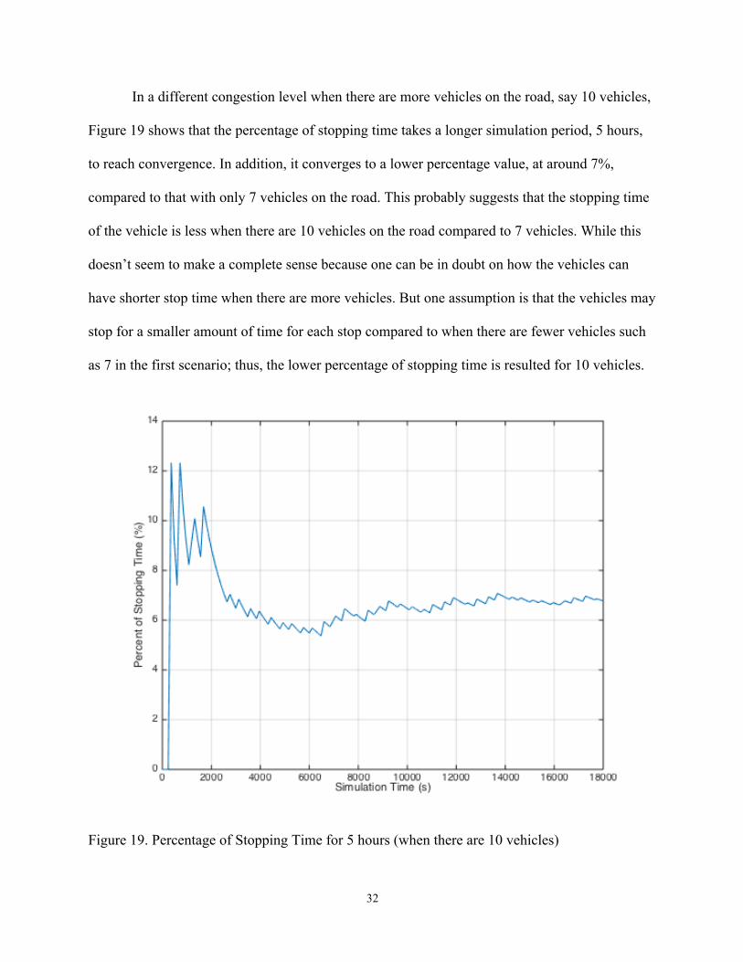
In a different congestion level when there are more vehicles on the road, say 10 vehicles,

Figure 19 shows that the percentage of stopping time takes a longer simulation period, 5 hours,

to reach convergence. In addition, it converges to a lower percentage value, at around 7%,

compared to that with only 7 vehicles on the road. This probably suggests that the stopping time

of the vehicle is less when there are 10 vehicles on the road compared to 7 vehicles. While this

doesn’t seem to make a complete sense because one can be in doubt on how the vehicles can

have shorter stop time when there are more vehicles. But one assumption is that the vehicles may

stop for a smaller amount of time for each stop compared to when there are fewer vehicles such

as 7 in the first scenario; thus, the lower percentage of stopping time is resulted for 10 vehicles.

Figure 19. Percentage of Stopping Time for 5 hours (when there are 10 vehicles)

33

However, in another congestion level with 15 vehicles on the ring road, no convergence

can be achieved even though the simulation for ran as long as 12 hours. This shows that higher

congestion level will have a stopping time that is more varied, but the percentage of stopping

time still wavers around 6%, which is also less than the percentage when there are only 7

vehicles.

Figure 20. Percentage of Stopping Time for 12 hours (when there are 15 vehicles)

34

Chapter 6 Conclusion and Future Work

In this thesis, a signalized ring road with traffic flow reproduced by the modified OV

model is simulated using MATLAB. By calculating the acceleration and determining the beacon

vehicle, which is the first vehicle closest to the stop line within the dilemma zone, it can be

observed from the velocity and location trajectories that there is no collision and not all vehicles

have to stop in a traffic cycle. This suggests that it is possible to avoid collisions even under the

effect of the dilemma zone. However, only the pre-timed signal is simulated in this thesis

because of the simplicity of the implementation. Thus, there can be a lot of variations to this

scenario that can be expanded on and improved as future studies.

First, implementing the pre-timed signal in CodeSkulpter as did in the scenario with no

traffic signal can be a step towards improvement. It helps to provide graphic results and to verify

the validity of the MATLAB coding that has questionable results. Second, conducting a

frequency analysis on how often vehicle stop in a traffic cycle can be another approach. This is

actually an extension to the percentage of stopping time that was analyzed in the previous

chapter. It can be used to determine if there is any repetitive or asymptotic traffic pattern and it

can be beneficial for traffic engineers to explore it for redesigning a signalized intersection.

Another approach is modifying the characteristics of the vehicle and the road, or even including

the many congestion levels by adding or subtracting the number of vehicles. By including more

scenarios, it can better demonstrate the randomness and dynamics in the real world. In addition,

observing other car-following models such as the Gipps model and more complicated road

networks can better represent the real-time traffics and provide more relevant results for realistic

applications.

35

Not only so, looking at the feasibility of the OV car-following model in a ring road with

actuated signals can be another option. Since the actuated signal responds to real-time traffic, the

randomness of the parameters as well as the drivers’ response may actually be beneficial to

incorporate signal to vehicle communications in order to smooth the vehicle’s trajectory. For

instance, when a vehicle approaches an intersection, it will try to ask for a change of traffic

signal for it to pass. If it is granted, the traffic light will change to green accordingly but if not, it

will tell the vehicle to slow down. This can reduce the stop-and-go behavior and minimize the

number of stops that the drivers have to face. It may actually be practical for the application of

the vehicle-to-infrastructure (V2I) and vehicle-to-vehicle (V2V) communication systems

discussed previously, which have the potential to reduce the risks of red-light violation and rear-

end accidents. Because of the fundamentals that this thesis focuses on, there are many future

directions that this thesis can take.

While this study does not directly suggest solutions to eliminate the dilemma zone, there

are potential applications that this study can be used for. In fact, because the initial speed and the

acceleration are known, this study may actually reproduce the approach suggested by Liu et al.

(1996) [8] to calculate and test the yellow interval timing in order to reduce or eliminate the

dilemma zone. This thesis seeks to identify the problem with signalized intersection, mainly the

problem with the dilemma zone, and though may not provide practical solutions to the problems

that occurred at signalized intersection, it will help stimulate other researchers on the topic and

suggest some potential applications relating to recent technology that may mitigate the dilemma

zone problems. This and future studies would help to understand the complexity of the yellow

light dilemma zone and eventually lead to a safe driving environment.

36

Chapter 7 Bibliography

1. FHWA Safety Program. Signalized Intersections: An Informational Guide. FHWA-SA-13-

027. http://safety.fhwa.dot.gov/intersection/signalized/13027/. Accessed July 30, 2015.

2. FHWA. Traffic Signal Timing Manual. FHWA-HOP-08-024.

http://ops.fhwa.dot.gov/publications/fhwahop08024/index.htm. Accessed July 30, 2015.

3. Gazis, D., R. Herman, and A. Mardudin. The Problem of the Amber Signal Light in Traffic

Flow. Operations Research: Vol. 8, No. 1, 112–132, January–February 1960.

4. Yan, X., E. Radwan, and M. Abdel-Aty. Characteristics of rear-end accidents at signalized

intersections using multiple logistic regression model. Accident Analysis & Prevention: Vol.

37, No. 6, November 2005, pp. 983-995.

5. Elmitiny, N., X. Yan, E. Radwan, C. Russo, and D. Nashar. Classification analysis of

driver’s stop/go decision and red-light violation. Accident Analysis & Prevention: Vol. 42,

No. 1, January 2010, pp. 101-111.

6. Zimmerman, K., and J. Bonneson. Intersection Safety at High-Speed Signalized

Intersections: Number of Vehicles in Dilemma Zone as Potential Measure. In Transportation

Research Record: Journal of the Transportation Research Board, No. 1897, Transportation

Research Board of the National Academies, Washington, D.C., 2004, pp. 126-133.

7. Bonneson, J., and K. Zimmerman. Effect of Yellow-Interval Timing on the Frequency of

Red-Light Violations at Urban Intersections. In Transportation Research Record: Journal of

the Transportation Research Board, No. 1865, Transportation Research Board of the

National Academies, Washington, D.C., 2004, pp. 20-27.

8. Liu, C., R. Herman, and D. C. Gazis. A Review of the Yellow Interval Dilemma.

Transportation Research Part A: Policy and Practice, Vol. 30, 1996, pp. 333-348.

37

9. Liu, Y., G-L Chang, R. Tao, T. Hicks, and E. Tabacek. Empirical Observations of Dynamic

Dilemma Zones at Signalized Intersections. In Transportation Research Record: Journal of

the Transportation Research Board, No. 2035, Transportation Research Board of the

National Academies, Washington, D.C., 2007, pp. 122-133.

10. Zimmerman, K., D. Tolani, R. Xu, T. Qian, and P. Huang. Detection, Control, and Warning

System for Mitigating Dilemma Zone Problem. In Transportation Research Record: Journal

of the Transportation Research Board, No. 2298, Transportation Research Board of the

National Academies, Washington, D.C., 2012, pp. 30-37.

11. M. Bando, K. Hasebe, A. Nakayama, A. Shibata, and Y. Sugiyama. Structural Stability of

Congestion in Traffic Dynamics. Japan Journal of Industrial and Applied Mathematics, Vol.

11, 1994, pp. 203-223.

12. M. Bando, K. Hasebe, A. Nakayama, A. Shibata, and Y. Sugiyama. Dynamical model of

traffic congestion and numerical simulation. Physics Review E, Vol. 51, 1995, pp. 1035-

1042.

13. M. Bando, K. Hasebe, K. Nakanishi, and A. Nakayama. Analysis of optimal velocity model

with explicit delay. Physics Review E, Vol. 58, 1998, pp. 5429-5435.

14. Greiner, J. Documentation of CodeSkulptor. Rice University.

http://www.codeskulptor.org/docs.html. Accessed August 8, 2015.

15. USDOT. Intelligent Transportation Systems Joint Program Office. Vehicle-to-Infrastructure

(V2I) Communications for Safety. http://www.its.dot.gov/safety/v2i_comm_safety.htm.

Accessed August 8, 2015.

16. USDOT. Intelligent Transportation Systems Joint Program Office. Vehicle-to-Vehicle (V2V)

Communications for Safety. http://www.its.dot.gov/safety/v2v_comm_safety.htm. Accessed

August 8, 2015.

38

Chapter 8 Appendix

Chapter 8.1 Programming Codes in MATLAB

Chapter 8.1a Snippets of OV Model Function function acc_f = OV_Model(clearance, v_n1) %original OV acc_OV = 1/REACTION_T * (min(V_F, clearance / TAU) - v_n1); %modified OV, bounded acceleration acc_1 = min(MAX_ACC, acc_OV); %modified OV, collision-free s0 = sqrt(2 * clearance / MIN_ACC); acc_2 = 2/TIME_STEP^2 * (clearance - v_n1 * TIME_STEP - 1/2 * MIN_ACC * (TIME_STEP - s0)^2); %modified OV, no negative speed acc_3 = min(acc_2, acc_1); acc_f = max(-v_n1/ TIME_STEP, acc_1);

Chapter 8.1b Snippets of Car Spawner Function function car_array = car_spawner( num_of_car, MAX_VEL, MIN_VEL, ROAD_LEN ) %car_array is a 2D array with multiple cars and their respective char % [ [1, loc_1, vel_1, acc_1] % [2, loc_2, vel_2, acc_2]...] car_array = []; R = ROAD_LEN / (2*pi); %2*pi*R = circumference for i = 0:num_of_car - 1 car_vel = MIN_VEL + (MAX_VEL - MIN_VEL)*rand(1,1); car_array = vertcat(car_array, [i + 1, (2 * pi * (num_of_car - i) / num_of_car) * R, car_vel, 0]); end

Chapter 8.1c Snippets of Car Update Function %Main algorithm for the Ring Road with No Traffic Signal function [] = car_update() car_array = car_spawner(num_of_car, MAX_VEL, MIN_VEL, ROAD_LEN); for j = 1:SIM_TIME/TIME_STEP %simulation time of 30 seconds for i = 1:num_of_car

39

if i == 1 clearance = car_array(end, 2) - car_array(1, 2) - JAM_SPACING; clearance = clearance + ROAD_LEN; else clearance = car_array(i - 1, 2) - car_array(i, 2) - JAM_SPACING; end car_array(i, 4) = OV_Model(clearance, car_array(i, 3)); car_array(i, 3) = car_array(i, 3) + car_array(i, 4) * TIME_STEP; car_array(i, 2) = car_array(i, 2) + TIME_STEP * car_array(i, 3);

end end

Chapter 8.1d Snippets of Find Beacon Vehicle Function %Supporting Algorithm to find the beacon vehicle for the Ring Road with Traffic Signal function ind = find_beacon(num_of_car, car_array, MU, G, REACTION_T, ROAD_LEN) for i = 1:num_of_car if car_array(i, 2) > ROAD_LEN car_array(i, 2) = mod(car_array(i, 2), ROAD_LEN); end end sorted_car_loc = sortrows(car_array, 2); for i = 1:num_of_car d_stop = sorted_car_loc(i, 3)^2 / (2 * MU * G); d_total = REACTION_T * sorted_car_loc(i, 3) + d_stop; if sorted_car_loc(i, 2) < 5000 - d_total I = find(car_array == sorted_car_loc(i)); ind = I; break else ind = -1; end end end

Chapter 8.1e Snippets of Pre-timed Signal Function %Main algorithm for the Ring Road with Pretimed Traffic Signal function [] = pretimed_signal_tester() %signal timing, concept of dillema zone GREEN = 23; YELLOW = 3;

40

RED = 32; ALL_RED = 2; ARYG = GREEN + YELLOW + RED + ALL_RED; %SIGNAL INDICATOR signal_bef = 'R'; signal_now = 'G'; car_array = car_spawner(num_of_car, MAX_VEL, MIN_VEL, ROAD_LEN); for j = 1:SIM_TIME/TIME_STEP %%step 1: light change if mod(j, ARYG) == mod(GREEN, ARYG) signal_bef = 'G'; signal_now = 'Y'; ind = find_beacon(num_of_car, car_array, MU, G, REACTION_T, ROAD_LEN); elseif mod(j, ARYG) == mod(0, ARYG) signal_bef = 'R'; signal_now = 'G'; end if signal_bef == 'G' && signal_now == 'Y' ind = ind; elseif signal_bef == 'R' && signal_now == 'G' ind = -1; end for i = 1:num_of_car if i == ind clearance = 0 - mod(car_array(ind, 2), ROAD_LEN); elseif i == 1 clearance = car_array(end, 2) - car_array(1, 2) - JAM_SPACING; clearance = clearance + ROAD_LEN; else clearance = car_array(i - 1, 2) - car_array(i, 2) - JAM_SPACING; end %update acceleration, speed, distance car_array(i, 4) = OV_Model(clearance, car_array(i, 3)); car_array(i, 3) = car_array(i, 3) + car_array(i, 4) * TIME_STEP; car_array(i, 2) = car_array(i, 2) + TIME_STEP * car_array(i, 3); end if car_array(1, 3) == 0 stopping_time = stopping_time + 1; end if j == multiplier * 100 multiplier = multiplier + 1; stopping_time_1 = horzcat(stopping_time_1, stopping_time/j * 100); end end

41

Chapter 8.2 Programming Codes in CodeSkulptor

The following codes are shown to support the implementation section of the Ring Road with no traffic signal. It can be ran directly from http://www.codeskulptor.org/#user40_yY3W3GEx5r_37.py if the readers would like to see the simulation or to modify the parameters for their own experiments.

# Ring Road Simulation # OV car following model, max/min accel, no negative velocities, collision free import simplegui import math import random # Parameters sim_time = 0 NUM_OF_CARS = 7 WIDTH = 600 HEIGHT = 600 started = False car_group = [] # Ring Road Characteristics ROAD_LEN = 5000 #ft R = ROAD_LEN / (2*math.pi) #2*pi*R = circumference CIRCLE_R = 200 #radius # Car Characteristics JAM_SPACING = 25 #ft JAM_ANG = JAM_SPACING / R MAX_ACC = 9.8425 #ft/s^2 MIN_ACC = 13.1234 #deceleration V_F = 65 #free flow speed ft/s MAX_VEL = 66 #max vehicle speed ft/s MIN_VEL = 22 #min vehicle speed ft/s TAU = 1.6 #time gap (s) REACTION_T = 1.2 #s TIME_STEP = 1.2 #delta t (s) TXT_OFFSET_Y = 15 DISPLAY_TIME = 1.2 ## default class to process image infor class ImageInfo: def __init__(self, center, size, dim = None):

42

self.center = center self.size = size self.dim = dim def get_center(self): return self.center def get_size(self): return self.size def get_dim(self): return self.dim # Car images properties blue_car_image = simplegui.load_image("http://images.clipartpanda.com/cars-20clipart-niBGKE66T.png") car_info = ImageInfo([588/2, 253/2], [588, 253], [30, 10]) ## define Car attributes and functions class Car: def __init__(self, index, loc, vel, acc, image, info): self.index = index self.pos = [WIDTH/2+CIRCLE_R*math.cos(loc/R),HEIGHT/2+CIRCLE_R*math.sin(loc/R)] self.loc = loc self.vel = vel self.acc = acc self.image = image self.image_center = info.get_center() self.image_size = info.get_size() def draw(self, canvas): canvas.draw_image(self.image, self.image_center, self.image_size, self.pos, [JAM_ANG*CIRCLE_R*6,JAM_ANG*CIRCLE_R*3], self.loc/R+math.pi/2) canvas.draw_text(str(self.index), self.pos, 20, 'Yellow','serif') ## update velocity, location, position of the vehicle def update(self): self.vel += self.acc * TIME_STEP self.loc += self.vel * TIME_STEP self.pos[0] = WIDTH/2 + CIRCLE_R * math.cos(self.loc/R) self.pos[1] = HEIGHT/2 + CIRCLE_R * math.sin(self.loc/R) ## spawn the number of cars inputted def car_spawner():

43

global car_group for i in range(NUM_OF_CARS): car_vel = random.randint(MIN_VEL, MAX_VEL) car_group.append(Car(i + 1, (2 * math.pi * (NUM_OF_CARS-i) / NUM_OF_CARS) * R, car_vel, 0, blue_car_image, car_info)) ## define OV model equations to get acceleration def OV(clearance, v_n1): acc_OV = 1.0/REACTION_T * (min(V_F, clearance / TAU) - v_n1) #original OV, use float in division acc_1 = min(MAX_ACC, acc_OV) #modified OV, bounded acceleration s0 = math.sqrt(2 * clearance / MIN_ACC) #modified OV, collision-free acc_2 = 2 / math.pow(TIME_STEP, 2) * (clearance - v_n1 * TIME_STEP - 1/2 * MIN_ACC * math.pow((TIME_STEP - s0), 2)) acc_3 = min(acc_2, acc_1) acc_f = max(-v_n1/ TIME_STEP, acc_1) #modified OV, no negative speed return acc_f ## define when and how to update car movements def car_update(canvas): global car_group, sim_time if started: #for j in range(int(30/TIME_STEP)): for i in range(NUM_OF_CARS): clearance = car_group[i-1].loc - car_group[i].loc - JAM_SPACING ## special case for the first vehicle if i == 0: clearance += ROAD_LEN car_group[i].acc = OV(clearance, car_group[i].vel) car_group[i].update() car_group[i].draw(canvas) sim_time += TIME_STEP ## print out data for drawing speed/trajectory diagram on excel (first 30 seconds of

44

simulation) if sim_time <= 30.1: for i in range(NUM_OF_CARS): print str(car_group[i].vel) print str(car_group[i].loc) else: for i in car_group: i.draw(canvas) print str(i.loc) car_spawner() # Handler to draw on canvas def draw(canvas): #ring road canvas.draw_circle([WIDTH/2, HEIGHT/2], CIRCLE_R, 5, "WHITE") #car car_update(canvas) #show current parameters canvas.draw_text("Simulation time: " + str(sim_time) + " s", [20, 30], 15, "WHITE") canvas.draw_text("Number of Cars Spawned: " + str(NUM_OF_CARS), [20, 30 + TXT_OFFSET_Y], 15, "WHITE") canvas.draw_text("First vehicle's speed: " + str(car_group[0].vel), [20, 30 + 2*TXT_OFFSET_Y], 15, "WHITE") ## Update Simulation Time def tick(): global sim_time if started: sim_time += 0 def format_time(time): milli = time % 10 sec = time // 10 return str(sec) + "." + str(milli) def click(): global started timer.start() started = True def pause(): global started

45

timer.stop() started = False ## Create timer timer = simplegui.create_timer(100, tick) #interval = 100 millisecond = 0.1 second # Create a frame and assign callbacks to event handlers frame = simplegui.create_frame("Ring Road Simulation", WIDTH, HEIGHT) frame.set_draw_handler(draw) frame.add_button("Start Simulation", click) frame.add_button("Pause Simulation", pause) # Start the frame animation frame.start()