resilience thinking and structured decision making in
TRANSCRIPT
University of Nebraska - LincolnDigitalCommons@University of Nebraska - Lincoln
Dissertations & Theses in Natural Resources Natural Resources, School of
8-2015
Resilience Thinking and Structured DecisionMaking in Social-Ecological SystemsNoelle M. HartUniversity of Nebraska-Lincoln, [email protected]
Follow this and additional works at: http://digitalcommons.unl.edu/natresdiss
Part of the Terrestrial and Aquatic Ecology Commons
This Article is brought to you for free and open access by the Natural Resources, School of at DigitalCommons@University of Nebraska - Lincoln. Ithas been accepted for inclusion in Dissertations & Theses in Natural Resources by an authorized administrator of DigitalCommons@University ofNebraska - Lincoln.
Hart, Noelle M., "Resilience Thinking and Structured Decision Making in Social-Ecological Systems" (2015). Dissertations & Theses inNatural Resources. Paper 118.http://digitalcommons.unl.edu/natresdiss/118

RESILIENCE THINKING AND STRUCTURED DECISION MAKING
IN SOCIAL-ECOLOGICAL SYSTEMS
by
Noelle M. Hart
A DISSERTATION
Presented to the Faculty of
The Graduate College at the University of Nebraska
In Partial Fulfillment of Requirements
For the Degree of Doctor of Philosophy
Major: Natural Resource Sciences
(Adaptive Management)
Under the Supervision of Professor Craig R. Allen
Lincoln, Nebraska
August, 2015
RESILIENCE THINKING AND STRUCTURED DECISION MAKING
IN SOCIAL-ECOLOGICAL SYSTEMS
Noelle M. Hart, Ph.D.
University of Nebraska, 2015
Adviser: Craig R. Allen
Natural resource management may be improved by synthesizing approaches for
framing and addressing complex social-ecological issues. This dissertation examines how
structured decision making processes, including adaptive management, can incorporate
resilience thinking. Structured decision making is a process for establishing a solid
understanding of the problem, values, management options, and potential consequences.
Adaptive management is a form of structured decision making in which uncertainty is
reduced for iterative decisions through designed monitoring and review. Resilience
thinking can help conceptualize complex social-ecological systems and draws attention to
the risks of managing for narrowly-focused objectives.
This dissertation provides practical advice to managers and can facilitate
discussions regarding how to make wise decisions in complex social-ecological systems.
Specifically, I explore how an iterative structured decision making process can contribute
to the resilience of an oak forest in southeastern Nebraska. Chapter 2 discusses how a
structured decision making process can emphasize principles of resilience thinking. I
present a suite of management recommendations, drawing on information from
practitioners’ guides and using oak forest conservation as a case study. Chapter 3
demonstrates how oak forest models can reflect elements of resilience thinking and be
used to identify optimal policies. I quantify a state-and-transition model into a Markov
decision process by establishing transition probabilities based on resilience assumptions
and setting the time horizon (infinite), discount factor, and reward function. Limitations
are discussed, including that the optimal policy is sensitive to uncertainty about aspects of
the Markov decision process. Chapter 4 provides a practical method for incorporating
adaptive management projects into State Wildlife Action Plans, in part based on
experience with conservation planning in Nebraska. I present a dichotomous key for
identifying when to use adaptive management and a basic introduction to developing
adaptive management projects are presented. Chapter 5 describes an initial effort to
reduce uncertainty for oak forest conservation in southeastern Nebraska. I use multimodel
inference to explore different hypotheses about what environmental and management
variables are correlated with oak seedling abundance. The results indicate that the
number of large oaks is an important factor. I discuss adaptive management as a potential
means for further investigating management effects. Chapter 6 synthesizes the
dissertation by considering the management implications for oak forest conservation in
southeastern Nebraska, identifying general challenges and limitations, presenting
methods for improving the framework, and returning to the broader goal of implementing
the social-ecological systems paradigm.
iv
AUTHOR’S ACKNOWLEDGEMENTS
I would like to thank Craig R. Allen (adviser) and Melinda Harm Benson (co-
adviser) for dedicating time and effort toward leading a student fresh out of
undergraduate through the completion of a dissertation. I would also like to thank the rest
of my committee: Andrew J. Tyre, Erin E. Blankenship, and B. Ken Williams. Drew
helped me recognize the potential and limitations of quantitative modeling to inform
natural resource decision problems. Erin very patiently guided me as I sought to increase
my understanding of statistics. Ken challenged me to think critically about how my work
connects to past, present, and prospective future of conservation science and
management.
Support from professors, staff, and fellow graduate students connected to the NSF
IGERT program and the Nebraska Cooperative Fish and Wildlife Research Unit was
integral to my success. Graduate school would have been a lonely, confusing experience
without their friendship and mentoring. I would especially like to acknowledge Valerie
Egger and Caryl Cashmere for their dedication to helping students meet administrative
requirements, and Dan Uden and Kent Fricke for exchanging their ideas and insights
throughout the development of my dissertation. In addition, I couldn’t have asked for a
better fieldwork partner than Dan, with his boundless goodwill and energy.
I would like to thank Kristal Stoner, Rick Schneider, Melissa Panella, Krista
Lang, Jordan Marquis, Kent Pfeiffer, and Gerry Steinauer for their contributions to the
Nebraska Natural Legacy Project portion of my dissertation. Thank you also to Michelle
Hellman for meandering over tough terrain with us while we sorted out methodological
details (like how to navigate back to the car).

v
Grants from the National Science Foundation Integrated Graduate Education and
Research Traineeship (DGE-0903469) and the Nebraska Natural Legacy Project funded
my graduate education and scientific endeavors. Thank you to the organizations and
individuals who expressed belief in me and my research ideas through these awards.
And finally, a hearty thank you to my many friends and family members for
reminding me what is truly important in life. I am grateful to my husband, Kerry, for
being the understanding, encouraging partner I needed to endure the emotional
rollercoaster that is graduate school. My parents have been ever supportive, and every
milestone in my life has been made possible in part by their love and unwavering
confidence in my abilities.
vi
TABLE OF CONTENTS
AUTHOR’S ACKNOWLEDGEMENTS .......................................................................... iv
LIST OF FIGURES ............................................................................................................ x
LIST OF TABLES ............................................................................................................ xv
CHAPTER 1. INTRODUCTION .......................................................................................1
1. BACKGROUND: RESILIENCE AND STRUCTURED DECISION MAKING
..................................................................................................................................2
1.1 Resilience ..............................................................................................2
1.2 Structured Decision Making ..................................................................7
2. PURPOSE .........................................................................................................12
3. LITERATURE CITED ......................................................................................13
CHAPTER 2. RESILIENCE THINKING LINKED TO STRUCTURED DECISION
MAKING – A FRAMEWORK FOR INCORPORATING RESILIENCE INTO
NATURAL RESOURCE MANAGEMENT ....................................................................18
1. INTRODUCTION ............................................................................................18
2. RESILIENCE THINKING ...............................................................................20
3. STRUCTURED DECISION MAKING ...........................................................22
4. INTEGRATING RESILIENCE THINKING INTO STRUCTURED
DECISION MAKING ...........................................................................................25
4.1 Problem ................................................................................................25
4.2 Objectives ............................................................................................28
4.3 Alternatives ..........................................................................................33
4.4 Consequences .......................................................................................35
4.5 Tradeoffs ..............................................................................................37
4.6 Monitoring and review .........................................................................39
5. CASE STUDY: OAK FOREST CONSERVATION IN SOUTHEASTERN
NEBRASKA ..........................................................................................................41
5.1 Case study: Problem ............................................................................42
5.2 Case study: Objectives ........................................................................45
vii
5.3 Case study: Alternatives .....................................................................46
5.4 Case study: Consequences ...................................................................47
5.5 Case study: Tradeoffs ..........................................................................47
5.6 Case study: Monitoring and review .....................................................48
6. CONCLUSION ..................................................................................................49
7. LITERATURE CITED ......................................................................................50
8. APPENDIX: Suggested readings .......................................................................76
CHAPTER 3. OPTIMIZATION AND RESILIENCE THINKING FOR
MANAGEMENT OF A HYPOTHETICAL MIDWESTERN OAK FOREST ................79
1. INTRODUCTION .............................................................................................79
2. BACKGROUND ...............................................................................................81
3. STATE-AND-TRANSITION MODEL AND MANAGEMENT OPTIONS ...82
4. MARKOV DECISION PROCESSES ...............................................................83
4.1 Time horizon and discount factor ........................................................85
4.2 Transition probabilities ........................................................................86
4.3 Single unit: Model description .............................................................88
4.4 Single unit: Results ..............................................................................89
4.5 Single unit: Interpretation ....................................................................90
4.6 Multiple units: Model description ........................................................92
4.7 Multiple units: Results .........................................................................93
4.8 Multiple units: Interpretation ...............................................................95
5. UNCERTAINTY AND SENSITIVITY ANALYSIS .......................................97
5.1 Incorporating parameter uncertainty ....................................................97
5.1.1 Alternative transition matrices ..............................................97
5.1.2 Sensitivity to transition probabilities: results and
interpretation ..................................................................................98
5.2 Different objectives and weightings ..................................................100
5.2.1 Alternative state returns ......................................................100
5.2.2 Sensitivity to state returns: results and interpretation .........101
viii
5.2.3 Alternative discount factors ................................................103
5.2.4 Sensitivity to discount factor: results and interpretation.....103
6. CONCLUSION ................................................................................................105
7. LITERATURE CITED ....................................................................................109
CHAPTER 4. INCORPORATING ADAPTIVE MNAGEMENT INTO STATE
WILDLIFE ACTION PLANS .........................................................................................141
1. INTRODUCTION ...........................................................................................141
2. BRIEF OVERVIEW OF STRUCTURED DECISION MAKING AND
ADAPTIVE MANAGEMENT ............................................................................143
3. WHEN TO USE ADAPTIVE MANAGEMENT FOR A STATE WILDLIFE
ACTION PLAN ...................................................................................................145
4. HOW TO DRAFT ADAPTIVE MANAGEMENT PROJECTS FOR A STATE
WILDLIFE ACTION PLAN ..............................................................................147
4.1 Involve the right people .....................................................................147
4.2 Prioritize uncertainties ......................................................................148
4.3 Choose how to learn...........................................................................149
4.4 Represent hypotheses with models ....................................................149
4.5 Discuss and set standards for convincing evidence ...........................150
4.6 Make it happen ...................................................................................151
4.7 Keep it going ......................................................................................151
4.8 Decide when to assess and revise, or get out .....................................152
5. CASE STUDY: THE NEBRASKA NATURAL LEGACY PROJECT .........153
5.1 Nebraska Natural Legacy Project and structured decision making ...153
5.2 When to use adaptive management within the Nebraska Natural
Legacy Project .........................................................................................156
5.3 How to draft adaptive management projects within the Nebraska
Natural Legacy Project ............................................................................158
6. CONCLUSION ................................................................................................161
7. LITERATURE CITED ....................................................................................163
CHAPTER 5. REDUCING UNCERTAINTY ABOUT OAK SEEDLING
ABUNDANCE TO IMPROVE CONSERVATION OF OAK-DOMINATED FORESTS

ix
..........................................................................................................................................175
1. INTRODUCTION ...........................................................................................175
2. STUDY SITE AND DATA COLLECTION ...................................................177
3. RESPONSE VARIABLE AND COVARIATES ............................................178
4. STATISTICAL METHODS ............................................................................181
5. RESULTS ........................................................................................................182
6. DISCUSSION ..................................................................................................183
7. ADAPTIVE MANAGEMENT POTENTIAL .................................................184
8. CONCLUSION ................................................................................................185
9. LITERATURE CITED ....................................................................................186
CHAPTER 6: CONCLUSION ........................................................................................201
1. MANAGING INDIAN CAVE STATE PARK ...............................................202
2. GENERAL CHALLENGES AND LIMITATIONS .......................................206
3. IMPROVING THE FRAMEWORK ...............................................................208
4. CONCLUDING REMARKS ...........................................................................209

x
LIST OF FIGURES
Figure 2-1. Resilience thinking is a way of framing what is known about a given system,
while structured decision making offers a process for helping managers plan how to
address a given natural resource issue within the system. I propose a framework that links
the lessons and warnings of resilience thinking to the steps of structured decision making
as a way of developing transparent, defensible natural resource management plans that
enable systems to handle and adapt to disturbances. .........................................................55
Figure 2-2. Spiderweb diagrams offer a way of graphically representing consequences for
constructed performance measures based on properties of resilience. This method allows
for visual comparisons of alternatives in the context of general resilience, which can aid
in the assessment of tradeoffs. For example, decision makers can look at the area covered
and where peaks and valleys occur between alternatives. The diagrams above show the
hypothetical general resilience-related consequences for two alternatives (A and B).
Alternative B is more evenly spread and appears to cover more area, but there are places
where alternative A outperforms alternative B, such as for ecological variability and
innovation. Both alternatives have extreme high and low points, which may be
concerning depending on how strongly these performance measures are weighted by the
decision maker(s). ..............................................................................................................56
Figure 2-3. Resilience thinking requires acknowledging scales above and below the focal
scale. This diagram depicts different scales for the oak forest conservation problem at
Indian Cave State Park. The focal scale, forested areas of the park, is in bold. The focal
scale is nested within scales above (thinner solid outline) and contains scales below
(dashed outline). .................................................................................................................58
Figure 2-4. Ball-and-cup diagram of two alternative stable states (oak-attracted, shady-
attracted) for the forest system at Indian Cave State Park. Within the alternatives states,
the system can be (a) oak-dominated and recently burned, (b) oak-dominated and not
recently burned, (c) mixed oak and shade tree, or (d) shady. In the absence of fire, all else
being equal, the system is predicted to move from the oak-attracted state to the shady-
attracted state. The system exhibits hysteresis, such that it takes more effort to cross back
over the threshold from the shady-attracted state to the oak-attracted state than it does to
go from oak-attracted to shady-attracted; this is indicated by the deeper “cup” for the
shady-attracted state than the oak-attracted state. ..............................................................59
Figure 2-5. Objectives selected for the Indian Cave State Park structured decision making
process. Fundamental objectives appear in circles. Means objectives, whose achievement
contributes to the fundamental objectives, appear in rectangles. Dashed lines indicate
objectives for which decreases of the components are valued. In contrast, solid lines
typically indicating a desired increase, with the exception the components of general
resilience objectives, which do not easily lend themselves to a classification of desired
increase or decrease. NNLP = Nebraska Natural Legacy Project .....................................60

xi
Figure 2-6. Spiderweb diagrams of the general resilience constructed performance
measure scores for comparison across alternatives of the Indian Cave State Park
structured decision making process. The “state-based unit management” alternative
covers a comparatively high amount of area, has peaks in diversity, modularity, and
ecosystem services, and performs as well or better than the “state-based park
management” alternative for all the principles. The “experiment” and “intensive
management trial” alternatives scores comparatively low for ecosystem services and
ecological variability, but receives higher scores for humility and innovation than the
“state-based unit management” alternative. .......................................................................61
Figure 3-1. Resilience-based state-and-transition model developed following the
recommendations of Briske et al. (2008). The reference state (oak-attracted) is
characterized by numerous oaks and a relatively open midstory, is maintained by
feedback between fire and oaks, and can exist in a burned oak or unburned oak phase.
The unburned oak phase is at risk of transitioning into the alternative state (shady-
attracted), when decreased frequency of fire enables establishment of shade-tolerant trees.
The alternative state is maintained by feedbacks between low light availability and shade-
tolerant trees. The state can be in a mixed phase, with a dense midstory and some oaks, or
a shady phase, with a dense midstory and few or no oaks. Returning to the oak-attracted
state is only possible along the restoration pathway, which requires management input.
..........................................................................................................................................113
Figure 3-2. Markovian decision process for the oak forest conservation example. A given
area of the park (the entire park or an individual unit, for the single and multiple unit
models, respectively) can be classified as being in a burned oak, unburned oak, mixed, or
shady condition. Arrows represent potential transitions for a single time step (pij(a) > 0
for at least one action), with dotted arrows signifying transitions that are only possible
through management intervention (i.e., action other than “do nothing”). ......................114
Figure 3-3. For the single unit model of the oak forest conservation example, five
simulated time path trajectories for a time horizon of 25 years under three different sets
of transition matrices and assuming implementation of the optimal decision (based on an
infinite time horizon, discount factor = 0.95) at each time step. The “oak resilient” model
assumes that the unburned oak condition, and thereby the oak-attracted state, is more
resilient (i.e., less likely to transition into the shady-attracted state). The “mixed resistant”
model assumes that the mixed condition is less likely to transition into the shady
condition. Patterns are similar across the original, “oak resilient,” and “mixed resistant”
models, and include oscillation between burned and unburned oak and entering the shady
state permanently. Different colors represent different starting conditions. ....................115
Figure 3-4. For the multiple unit model of the oak forest conservation example, five
simulated time path trajectories for a time horizon of 25 years under the original set of
transition matrices and assuming implementation of the optimal decision (based on an
infinite time horizon, discount factor = 0.95) at each time step. Patterns include
oscillation between states 16 (1 burned oak, 2 unburned oak) and 19 (2 burned oak, 1
unburned oak), permanently entering state 1 (all 3 shady), and permanently entering state

xii
14 (1 burned oak, 1 unburned oak, 1 shady). However, in some cases, the system is able
to “escape” state 14 (1 burned oak, 1 unburned oak, 1 shady) and move to the oscillation.
Different colors represent different starting conditions. ..................................................116
Figure 3-5. For the multiple unit model of the oak forest conservation example, five
simulated time path trajectories for a time horizon of 25 years under the “oak resilient”
set of transition matrices (for which the unburned oak condition is less likely to transition
to the mixed condition) and assuming implementation of the optimal decision (based on
an infinite time horizon, discount factor = 0.95) at each time step. Patterns include
oscillation between states 16 (1 burned oak, 2 unburned oak) and 19 (2 burned oak, 1
unburned oak), permanently entering state 1 (all 3 shady), and permanently entering state
14 (1 burned oak, 1 unburned oak, 1 shady). However, in some cases, the system is able
to “escape” state 14 (1 burned oak, 1 unburned oak, 1 shady) and move to the oscillation.
Different colors represent different starting conditions. ..................................................117
Figure 3-6. For the multiple unit model of the oak forest conservation example, five
simulated time path trajectories for a time horizon of 25 years under the “mixed resistant”
set of transition matrices (for which the mixed condition is less likely to transition to the
shady condition) and assuming implementation of the optimal decision (based on an
infinite time horizon, discount factor = 0.95) at each time step. Patterns include
oscillation between states 16 (1 burned oak, 2 unburned oak) and 19 (2 burned oak, 1
unburned oak), permanently entering state 1 (all 3 shady), and permanently entering state
14 (1 burned oak, 1 unburned oak, 1 shady). However, in some cases, the system is able
to “escape” state 14 (1 burned oak, 1 unburned oak, 1 shady) and move to the oscillation.
Different colors represent different starting conditions. .................................................118
Figure 3-7. For the multiple unit model of the oak forest conservation example, five
simulated time path trajectories for a time horizon of 25 years under the “two-third not
shady” valuation (for which state returns exist as long at least two units are not in the
shady condition) and assuming implementation of the optimal decision (based on an
infinite time horizon, discount factor = 0.95) at each time step. Patterns include
oscillation between states 16 (1 burned oak, 2 unburned oak) and 19 (2 burned oak, 1
unburned oak), permanently entering state 1 (all 3 shady), and permanently entering state
14 (1 burned oak, 1 unburned oak, 1 shady). However, in some cases, the system is able
to “escape” state 14 (1 burned oak, 1 unburned oak, 1 shady) and move to the oscillation.
Different colors represent different starting conditions. ..................................................119
Figure 3-8. For the multiple unit model of the oak forest conservation example, five
simulated time path trajectories for a time horizon of 25 years under the “no shady”
valuation (for which state returns are equivalent and non-zero when no unit is shady, and
zero otherwise) and assuming implementation of the optimal decision (based on an
infinite time horizon, discount factor = 0.95) at each time step. Similar to the original
valuation results, patterns include an oscillation between states 16 (1 burned oak, 2
unburned oak) and 19 (2 burned oak, 1 unburned oak) and permanently entering state 1
(all 3 shady).Unlike the original valuation, there is no holding at state 14 (1 burned oak, 1
xiii
unburned oak, 1 shady), and there is a new oscillation between state 10 (3 unburned oak)
and state 20 (3 burned oak). Different colors represent different starting conditions.
..........................................................................................................................................120
Figure 3-9. Comparison of optimal policies across discount factors ranging from 0.90 to
0.99 at increments of 0.01 for the single unit model of the oak forest conservation
example, using the original transition probabilities and original valuation scheme. Light
gray boxes represent decisions that are identical to the results for a 0.95 discount factor.
Dark gray boxes indicate that the optimal decision is different for the particular state
when a given discount factor is used. In the single unit example, the optimal policy is the
same when the discount factor is between 0.90 and 0.98. When the discount factor is
equal to 0.99, the optimal decision for the shady state is different than the original result.
..........................................................................................................................................121
Figure 3-10. Comparison of optimal policies across discount factors ranging from 0.90 to
0.99 at increments of 0.01 for the multiple unit model of the oak forest conservation
example, using the original transition probabilities and original valuation scheme. Light
gray boxes represent decisions that are identical to the results for a 0.95 discount factor.
Dark gray boxes indicate that the optimal decision is different for the particular state
when a given discount factor is used. In the multiple unit example, the optimal decision is
different for at least one of the states for every discount factor (other than 0.95, of
course). There is a maximum of seven changes for a given discount factor, which occurs
for a discount factor of 0.99. ............................................................................................122
Figure 4-1. Systematic planning approach of the Nebraska Natural Legacy Project
(NNLP) in the context of structured decision making and adaptive management (a
specific type of structured decision making). The problem is determined by which species
are prioritized under the NNLP. Species targets make up fundamental objectives. Means
objectives are related to the reduction of threats and stressors to the species. Alternatives
can be built from the conservation strategies. The arrows leading off of the evaluation
step of adaptive management represent adjustment based on two loops of learning; single
loop learning changes implementation and the double loop learning alters the
fundamental elements of the decision framework. .........................................................168
Figure 4-2. Dichotomous key for determining when to consider using adaptive
management, given specified uncertainties and knowledge of the management context.
The first part of the key evaluates whether the uncertainty is appropriate for adaptive
management, such that the uncertainty could be reduced through designed monitoring
and review of management consequences. The second part of the key addresses whether
the knowledge gained would be useful. The third part of the key relates to whether it is
practically possible to reduce the uncertainty. Adaptive management is impossible or
unlikely to succeed if the answer to any of these questions is “no.” Potential reasons for
the answer being “no” are listed along the right-hand side of the key. ...........................169
Figure 5-1. Boxplot of oak seedling abundance within 4-m radius plot for 360 locations
sampled at Indian Cave State Park in southeastern Nebraska. .......................................189
xiv
Figure 5-2. Boxplot of the number of large oaks within 10-m radius plot for 360 locations
sampled at Indian Cave State Park in southeastern Nebraska. ........................................190
Figure 5-3. Boxplot of the number of small trees within 10-m radius plot for 360
locations sampled at Indian Cave State Park in southeastern Nebraska. .........................191
Figure 5-4. Scatterplot showing the degree of correlation between the number of large
oaks and the number of small trees within the 10-m radius plots for 360 locations
sampled at Indian Cave State Park in southeastern Nebraska. ........................................192
Figure 5-5. Plots of the relationships between the categorical covariates (times burned
pre-germination, total times burned, and edge) and numerical covariates (number of large
oaks, number of small trees). The results suggest that there are potentially important
differences in central tendency and variability when examining covariates in the context
of other covariates, which may impact effect estimates when included together in the oak
seedling abundance models..............................................................................................193
Figure 5-6. Plot of predicted oak seedling abundance based on the number of large oaks,
using the top model (oak seedling abundance ~ number of large oaks). Dashed lines
indicate the 95% confidence interval. The lines are not straight because the data is back-
transformed from the negative binomial generalized linear model. ................................195

xv
LIST OF TABLES
Table 2-1. The following is a summary of structured decision making guidance based on
[1] Hammond et al. (1999), [2] Gregory et al. (2012), and [3] Conroy and Peterson
(2013). For a review of the tools of structured decision making, readers are referred to
page 53 of Gregory et al. (2012). .......................................................................................63
Table 2-2. I propose a natural resource management planning framework based on steps
of structured decision making and incorporating resilience thinking. This table presents a
summary of recommendations for going through the process, built from guidance found
in structured decision making and resilience thinking literature for practitioners.............65
Table 2-3. Here I link the questions from the Resilience Alliance’s Workbook for
Practitioners (RA 2010) to the steps of structured decision making (indicated by an X in
the respective column), with short descriptions of why I believe the answers can inform
the particular step(s) of structured decision making. Pr = Problem, O = Objectives, A =
Alternatives, C = Consequences, T = Tradeoffs ................................................................68
Table 2-4. Walker and Salt (2012) and Biggs et al. (2015) proposed principles for
managing resilience. These principles can be used for the design of resilience thinking-
based objectives and alternatives. ......................................................................................71
Table 2-5. Preliminary attempt to develop constructed performance measures for general
resilience objective using the principles of resilience (Table 2-4) as applied to the Indian
Cave State Park oak conservation example. The scores for the performance measure are
relative and lie along a spectrum from 0 to 4, where 4 is the best possible score. The table
below describes the ends of the spectrum. The “Oak Forest Example” column briefly
discusses each principle in context of the case study. .......................................................72
Table 2-6. Descriptions of the alternatives under consideration for the Indian Cave State
Park oak forest example. The first two alternatives are variations of a state-based
management policy in which decisions are determined by the current state of the system.
The third alternative is a method for active learning about management impacts. The last
alternative is a combination of a state-based approach and a trial-and-error exploration of
intensive management. .......................................................................................................74
Table 2-7. Rapidly assessed consequences table for the Indian Cave State Park
management example, given the specified fundamental objectives and alternatives.
Consequences are described along a scale and represented by symbols (“++”, “+”, “~”, “-
”, “- -”), where a “+ +” indicates a relatively high level of predicted success in achieving
the objective and a “- -” indicates a low level of predicted success. As the purpose of the
example is to demonstrate what a structured decision making process integrating
resilience thinking might look like (rather than to present a precise description or
prescription of a real situation), how the consequences were determined is not important.
State-based unit management scores as well or better than all other alternatives, except
for the management cost objective. ...................................................................................75
xvi
Table 3-1. Original matrices of transition probabilities between conditions for a single
time step under each management action (pij(a)) of the oak forest conservation example.
..........................................................................................................................................123
Table 3-2. Rewards for a given time step, calculated as the return for the Markovian state
minus the cost of the management action, under the single unit example. Returns are
highest for the burned oak and unburned oak states and lowest for the shady state.
Management is cheapest for the do nothing action and most expensive for burning and
thinning. ...........................................................................................................................124
Table 3-3. For the single unit model of the oak forest conservation example, optimal
decision and expected value (infinite time horizon, discount = 0.95) for each state when
using the original set of transition probabilities matrices. The greatest expected value
occurs when the park exists in the burned oak state, with similar expected values for the
unburned oak state. Moderate expected values are anticipated when the park exists in the
mixed state. No value is expected when the park exists in the shady state. ....................125
Table 3-4. Returns for each of the states (uniquely identified by Ix) when the park is
divided into three units (multiple unit example) under three different valuation schemes.
The “original” valuation scheme is a modification of the returns for the single unit model,
with greater value placed on a mix of oak states. The “two-thirds not shady” valuation
scheme allows non-zero returns when only one unit is in the shady state. The “no shady”
valuation scheme assigns equivalent and non-zero state returns when no unit is shady,
and assigns a zero return otherwise. Values in bold differ from the original values. BO =
burned oak, UO = unburned oak, M = mixed, S = shady ................................................126
Table 3-5. Cost of management actions (as combinations of actions from the single unit
example, uniquely identified by Ax) based on the number of units treated for the multiple
unit model of the oak forest conservation example. Costs are assumed to be area-
dependent, such that the per unit cost is one-third the cost of the single unit model (per
unit costs: DN = 0, B = 1/3, T = 1, BT = 4/3). For each action combination (Ax), per unit
cost was multiple by the number of units applying the given action and then summed to
determine the total cost for the management of all three units. DN = Do nothing, B =
Burn, T = Thin, BT = Burn and thin ................................................................................127
Table 3-6. Expected values for optimal decision making for the multiple unit model of
the oak forest conservation example given three different sets of transition matrices. The
“oak resilient” set assumes that the unburned oak condition is less likely to transition to
the mixed condition, and the “mix resistant” set assumes that the mixed condition is less
likely to transition to the shady condition. Values in bold differ from the original. The
“oak resilient” transition matrices has the same expected values as the original, but the
“mixed resistant” matrices results in higher expected values in most cases. ...................128
Table 3-7. Optimal decisions for each state (Ix) of the multiple unit model (infinite time
horizon, discount = 0.95) when using the original transition matrices and valuation

xvii
scheme (same decisions for the “oak resilient” transition matrices). For a given state, the
number of units in each condition is the column sum, and the number of times an action
is applied is the row sum. BO = Burned Oak, UO = Unburned Oak, M = Mixed, S =
Shady, DN = Do Nothing, B = Burn, T = Thin, BT= Burn and Thin ..............................129
Table 3-8. “Oak resilient” transition matrices for the oak forest conservation example,
where “*_*” indicates the value deviates from the original. Compared to the original, the
probability of the unburned oak condition moving into the mixed state is lower, such that
the “oak-attracted” state is more resilient. .......................................................................130
Table 3-9. “Mixed resistant” transition matrices for the oak forest conservation example,
where “*_*” indicates the value deviates from the original. Compared to the original, the
probability of the mixed condition transitioning into the shady state is lower. ...............131
Table 3-10. Optimal decision and expected values for the single unit example of the oak
forest conservation example under the different transition matrices (original || oak
resilient || mixed resistant). The “oak resilient” set assumes that the unburned oak
condition is less likely to transition to the mixed condition, and the “mix resistant” set
assumes that the mixed condition is less likely to transition to the shady condition. All
optimal decisions are the same, and the only expected value that is different is for the
mixed condition under the mixed resistant matrices (in bold). .......................................132
Table 3-11. Optimal decisions for each state (Ix) (infinite time horizon, discount = 0.95)
for the multiple unit model using the “mixed resistant” transition matrices and original
valuation scheme. Underlined states indicate decisions different from the original. For a
given state, the number of units in each condition is the column sum, and the number of
times an action is applied is the row sum. BO = Burned Oak, UO = Unburned Oak, M =
Mixed, S = Shady, DN = Do Nothing, B = Burn, T = Thin, BT= Burn and Thin ...........133
Table 3-12. Optimal decisions for each state (Ix) (infinite time horizon, discount = 0.95)
for the multiple unit model using the original transition matrices and “two-thirds not
shady” valuation scheme. Underlined states indicate decisions different from the original.
For a given state, the number of units in each condition is the column sum, and the
number of times an action is applied is the row sum. BO = Burned Oak, UO = Unburned
Oak, M = Mixed, S = Shady, DN = Do Nothing, B = Burn, T = Thin, BT= Burn and Thin
..........................................................................................................................................134
Table 3-13. Expected values for the multiple unit model assuming implementation of the
optimal decision (infinite time horizon, discount = 0.95) and using the original transition
matrices and three different valuations schemes. The “two-thirds not shady” valuation
scheme allows non-zero returns when only one unit is shady. The “no shady” valuation
scheme assigns equivalent, non-zero state returns when no unit is shady, and assigns a
zero return otherwise. Expected values are general higher than the original under the
“two-thirds not shady” valuation scheme and lower for the “no shady” valuation scheme.
..........................................................................................................................................135

xviii
Table 3-14. Optimal decisions for each state (Ix) (infinite time horizon, discount = 0.95)
for the multiple unit model using the original transition matrices and “no shady”
valuation scheme. Underlined states indicate decisions different from the original. For a
given state, the number of units in each condition is the column sum, and the number of
times an action is applied is the row sum. BO = Burned Oak, UO = Unburned Oak, M =
Mixed, S = Shady, DN = Do Nothing, B = Burn, T = Thin, BT= Burn and Thin ...........136
Table 3-15. For the single unit model of the oak forest conservation example, comparison
of the optimal decision for a discount factor of 0.95 (original) and 0.99 (future reward
closer to present reward), under the original transition probabilities and valuation scheme.
The only difference in optimal decision occurs when in shady state, for which the
decision changes from “do nothing” to “burn and thin.” .................................................137
Table 3-16. For the multiple unit model of the oak forest conservation example,
comparison of the optimal decision for a discount factor of 0.95 (original) and 0.90
(future reward further discounted), under the original transition probabilities and
valuation scheme. States (Ix) that are not listed have the same decision as the original
multiple unit example. BO = Burned Oak, UO = Unburned Oak, M = Mixed, S = Shady,
DN = Do Nothing, B = Burn, T = Thin, BT= Burn and Thin ..........................................138
Table 3-17. For the multiple unit model of the oak forest conservation example,
comparison of the optimal decision for a discount factor of 0.95 (original) and 0.99
(future reward closer to present reward), under the original transition probabilities and
valuation scheme. States (Ix) that are not listed have the same decision as the original
multiple unit example. BO = Burned Oak, UO = Unburned Oak, M = Mixed, S = Shady,
DN = Do Nothing, B = Burn, T = Thin, BT= Burn and Thin ..........................................139
Table 3-18. Principles for resilient systems from Walker and Salt (2012) as related to the
hypothetical oak forest management example. ................................................................140
Table 4-1. Eight elements required by Congress to be included in State Wildlife Action
Plans. The elements can be readily incorporated into structured decision making and
adaptive management frameworks. .................................................................................170
Table 4-2. Types of uncertainty and scenarios that are not appropriate for adaptive
management, with examples relevant to State Wildlife Action Plans. ............................171
Table 4-3. Aspects of adaptive management (AM) project design with examples relevant
to State Wildlife Action Plans..........................................................................................172
Table 4-4. An abbreviated version of the target selection matrix tool used by the
Nebraska Natural Legacy Plan to guide choice of focal species within a biologically
unique landscape (BUL). Two species are included as examples. Scores are based upon
information previously gathered for the Nebraska Natural Legacy Project and stakeholder
input. The scoring results suggest that it may be more important to include Timber
xix
Rattlesnake than Wood Thrush in the set of targeted species, as this species is described
as more imperiled and habitat specific, while being equally endemic and BUL-dependent.
..........................................................................................................................................174
Table 5-1. Burning within management units at Indian Cave State Park, southeastern
Nebraska, can be classified as pre- and post-germination of oak seedlings following a
major mast year. Managers are specifically interested if the number of times burned pre-
germination and/or the number of times burned total (pre- and post-) are related to the
number of oak seedlings. The strong relationship between the numbers of times a unit has
been burned pre- and post-germination makes it possible to identify how many times a
site has been burned pre- and post- based on the number of times burned total (with an
exception for burned once). Interpretation of the number of times burned total by
combinations of times burned pre- and post-germination is presented in the table below,
along with the frequency of sites in each times burned total category. For example, if a
site has been burned a total of 5 times, then the site was burned four times pre-
germination and one time post-germination. ...................................................................196
Table 5-2. Model set of hypotheses about management and environmental variables
related to oak seedling abundance at Indian Cave State Park, southeastern Nebraska.
Following multimodel inference procedure, the AICc, delta AICc, and weights for each
model are provided. Models are order from lowest to highest AICc, such that models
towards the top of the list are better at explaining oak seedling abundance than models
further down the list. ........................................................................................................197
Table 5-3. Potential relationships between numerical covariates (number of small trees,
number of large oaks) and categorical covariates (times burned pre-germination, times
burned total, edge) and relationships among categorical covariates were examined.
Poisson generalized linear modeling was used for count data and binomial modeling for
edge data. Statistically significant effects at a 0.05 level (*) were detected in many cases.
..........................................................................................................................................198
Table 5-4. Model averaged covariate effect estimates averaged over the full set of models
(Table 5-2) with upper and lower bounds of the 95% confidence interval. Beyond the
intercept, the number of large oaks is the only covariate for which the 95% confidence
interval does not include 0. ..............................................................................................200
1
CHAPTER 1. INTRODUCTION
Under traditional natural resource management, policy makers viewed natural
resources as commodities to be controlled by managers for human use (Berkes 2010).
Today policy makers are favoring a different perspective focused on joint social-
ecological systems, interdisciplinary approaches, and a view that natural resources are a
source of ecosystem services and thereby human wellbeing (Millennium Ecosystem
Assessment 2003, Berkes 2010). This perspective fits well into the land ethics philosophy
espoused by Aldo Leopold (1949), who believed that role of humans in nature should be
as a “plain member and citizen of [the land-community]” rather than the “conqueror”
(Lee 1993). It is becoming increasingly clear that we value natural resources for more
than consumptive uses, and we never have enough knowledge of social-ecological
systems for perfect control and predictability.
Natural resource management theory has progressed, as evidenced by the
aforementioned paradigm shift, but implementing the modern social-ecological systems
perspective remains challenging and requires development of new ways of thinking and
making decisions. We must find ways to transcend the discussion of the benefits of a
complex social-ecological systems paradigm into actually making informed, defensible
decisions under difficult circumstances. We need to know: (a) how various proposed
approaches, or combinations of approaches (Polasky et al. 2011), influence the decision
making process and (b) under what circumstances decision makers should apply these
approaches.
In this dissertation, I use structured decision making as the backbone of natural
resource management planning. Structured decision making is a process for making

2
transparent, defensible decisions that explicitly outlines both values and consequences
(Hammond et al. 1999, Gregory and Keeney 2002, Gregory et al. 2012). Structured
decision making is different than science-based management (no mechanism for dealing
with values), consensus-based decision making (consensus as the goal), and
economic/multi-criteria decision techniques (expert-driven) (Gregory et al. 2012). The
foundational steps involve: 1) defining the problem, 2) determining objectives, 3)
outlining alternatives, 4) considering the consequences, and 5) understanding the
tradeoffs (Hammond et al. 1999). Adaptive management, a form of structured decision
making, uses monitoring and review in order to deliberately improve understanding of
the system and management outcomes (Walters 1986, Williams et al. 2002, Martin et al.
2009).
When facing issues in complex social-ecological systems, managers can apply
resilience thinking throughout structured decision making. Resilience thinking offers
ways of conceptualizing complex social-ecological systems characterized by alternative
states and non-linear transitions, and draws attention to the risks of managing for
narrowly-focused objectives. Structured decision making emphasizing resilience thinking
can help implement the modern social-ecological systems paradigm by creating a linkage
to actual natural resource management challenges and decisions.
1. BACKGROUND: RESILIENCE AND STRUCTURED DECISION MAKING
1.1 Resilience
Ecological resilience theory dates back to the early 1970’s when C. S. Holling
(1973) first described resilience as “a measure of the persistence of systems and of their

3
ability to absorb change and disturbance and still maintain the same relationships
between populations or state variables.” This emphasis on the amount of change that can
be absorbed before a transition occurs diverges from the traditional equilibrium-centered
view, which focused on stationarity and rate of return near an assumed equilibrium
(Holling 1973, Holling 1996). In the following, I summarize ideas generated by the
Holling school of resilience over the past forty years, recognizing that this necessarily
excludes numerous developments and critiques, such as the challenges of incorporating
social aspects (e.g., Folke 2006, Davidson 2010, Cote and Nightingale 2012) and links to
other schools of resilience (e.g., Walker and Salt 2012, Berkes and Ross 2013, Davidson
2013).
Resilience is a property of complex adaptive systems. Complex adaptive systems
consist of interconnected components operating around characteristic processes that
enable self-organization and adaptation in the face of internal or external perturbation
(Holling 2001, Biggs et al. 2012). There are multiple models theorizing the generation of
resilience within an ecosystem. Peterson et al. (1998) describe the breadth of these
models and propose a model that links ecological resilience, species richness, and scale.
The species diversity model (MacArthur 1955) suggests that resilience increases at a
constant rate with increasing biodiversity. The idiosyncratic model (Lawton 1994)
implies that resilience will be dependent upon the specific species present in the system.
The rivets model (Ehrlich and Ehrlich 1981) suggests that overlaps in function exist
between species, so not all species are necessary for overall function (though resilience
may be reduced by loss of species). The drivers and passengers model (Walker 1992)
suggests that resilience is determined by those species that most strongly influence
4
ecosystem dynamics. The cross-scale model proposed by Peterson et al. (1998)
hypothesizes that ecological resilience is derived from “overlapping function within
scales and reinforcement of function across scales.”
As implied by the cross-scale model of resilience, understanding scale in time and
space is critically important. Processes operating across time and space result in natural
discontinuities, for example clustered structural attributes such as body mass groups
(Allen et al. 2005). Interactions between slow and fast changing variables can result in
rapid large changes in ecosystem structure (Carpenter and Turner 2000). Examples of
systems with variables operating at different speeds include (1) a forest insect pest system
with fast-changing insect populations, intermediate-changing foliage, and slow-changing
trees, and (2) a human disease system with fast-changing infectious organisms,
intermediate-changing vectors and susceptible individuals, and a slow-changing human
population (Holling 1986).
Resilience also applies beyond ecology, recognizing that social systems impact
ecological systems and vice versa. Social aspects are considered an integral part of the
overall management system rather than an external driver (Folke 2006). Resilience theory
is strongly linked to social systems through concepts such as sustainability and
adaptability (Carpenter et al. 2001, Berkes et al. 2003, Walker et al. 2004, Davidson
2010). Sustainability implies a goal of maintaining a desirable state (Carpenter et al.
2001), or can be seen as a process capable of dealing with change (Berkes et al. 2003).
Adaptability is “the capacity of actors in a system to influence resilience”; in other words,
the ability for humans to manage resilience (Walker et al. 2004). As a result, resilience
5
thinkers tend to refer to social-ecological systems, rather than ecosystems or human
systems.
Social-ecological systems are complex adaptive systems made up of linked social
(e.g., community building, economic viability) and ecological (e.g., nutrient cycling,
biodiversity) components and processes (Biggs et al. 2012). These systems are dynamic
and generally tend to follow adaptive cycles, moving between growth, conservation,
collapse, and reorganization phases (Gunderson and Holling 2002, Walker et al. 2002).
Thresholds exist in social-ecological systems that, when crossed, can lead to rapid,
dramatic shifts from one stable state to another1. These thresholds may be related to
critical slow variables whose rate of change is slower than the management scale (Biggs
et al. 2012).
One critical challenge to implementing resilience thinking is identifying
thresholds. If quantification depends on understanding the effects of key drivers and
perturbations, we must have an idea of how much change can be absorbed before a
threshold is crossed. Groffman et al. (2006) offer one possible approach for investigating
thresholds. Focus on a particular ecosystem service of interest and then identify what
structures and functions influence the service. Those structures and functions are in turn
influenced by specific factors. Armed with this knowledge, one can then consider
whether those factors or their interactions exhibit a threshold response.
1 “State” (e.g., RA 2010), “regime” (e.g., Walker and Salt 2012), and “identity” (e.g., Cumming et al. 2005)
have all been used in the resilience literature to describe what characterizes where the system is now and
where it might transition to if a threshold is crossed. These words can take on multiple meanings depending
on discipline and context. For simplicity’s sake, we will refer to “states” characterized by components,
processes, and feedbacks identified during planning.
6
Resilience can be described as specified or general. Specified resilience involves
avoiding a particular threshold, so the objective is related to “resilience of what to what,”
where “to what” is a known disturbance (Carpenter et al. 2001). In contrast, general
resilience relates to how the system can handle disturbances, both known and unknown
(Walker and Salt 2012). A more generally resilient system is expected to absorb a
disturbance better than a less generally resilient system.
Managing for resilience requires openness of options, regional scale
considerations, focusing on heterogeneity, and acknowledging uncertainty and potential
surprises (Holling 1973). Variability is natural, and suppressing variability can ultimately
lead to unexpected and detrimental shifts (Holling and Meffe 1996). Disturbances are
critical as they can contribute to a system’s capacity to handle future surprises, such as
other disturbances, extreme conditions, or novel stresses. Disturbances can also, however,
bring systems closer to crossing a threshold into an alternative stable state. Disturbances
may be known or unknown, frequent or infrequent. In some cases, loss of historically
frequent disturbances can be seen as a “disturbance” itself, when the system evolved to
flourish under disturbance (Walker and Salt 2012, p. 49). Common examples of
management practices that reduce resilience include: (a) damming of rivers with naturally
high flow variability, (b) suppressing fire in fire-adapted regions, and (c) planting
monocultures in place of diverse plant communities (Holling and Meffe 1996). As
Peterson et al. (1998) point out, this type of management “channels ecological
productivity into a reduced number of ecological functions and eliminates ecological
functions at many scales” (p. 16).
7
Resilience management is a way to acknowledge and operate under intense
complexity. We live in a world of uncertainty, where non-linear changes, reflexive
human behavior to predictions, and rapidly altering systems make forecasting the future
incredibly challenging (Walker et al. 2002). Given severe limitations, we should use
management intervention to build capacity for systems to retain critical functions and
structures, rather than trying to reduce variability and maximize resource extraction
(Walker et al. 2002, Thrush et al. 2009). Walker et al. (2002) propose a resilience
management framework founded on the following assumptions: (1) thresholds and
hysteretic effects exist; (2) making extremely cautious decisions in the face of uncertainty
is a form of rigidity and therefore undermines resilience; (3) agents do not always
optimize income and social context matters; (4) market imperfections exist and are the
norm; (5) agents care about the process as well as the outcome; and (6) lack of property
rights for ecological goods and services means there are not markets.
1.2 Structured Decision Making
Structured decision making is a process for making transparent, defensible
decisions that explicitly outlines both values and consequences (Hammond et al. 1999,
Gregory and Keeney 2002, Gregory et al. 2012). The foundational steps involve: 1)
defining the problem, 2) determining objectives, 3) outlining alternatives, 4) considering
the consequences, and 5) understanding the tradeoffs (Hammond et al. 1999). Adaptive
management is a special form of structured decision making (Walters 1986, Williams et
al. 2002, Martin et al. 2009) and adds monitoring and review to the decision process.

8
Adaptive management is used to learn about management outcomes over time and adjust
management practices to reflect this learning.
In the following literature review, I focus specifically on adaptive management.
Given the emphasis resilience thinking places on the prevalence of uncertainty in
complex systems, adaptive management is a highly relevant structured decision making
framework for managing resilience. In addition, resilience and adaptive management
share a common foundation. Resilience was formally introduced in the literature by C. S.
Holling in 1973. Five years later, Holling (1978) described adaptive natural resource
management and referenced resilience. In 1993, Kai Lee’s book Compass and Gyroscope
pointed to adaptive management as a potential means to maintaining a desirable
equilibrium resilient to surprise.
Adaptive management of natural resources got its start in the 1970’s, described by
C. S. Holling (1978) in the seminal work Adaptive Environmental Assessment and
Management and furthered by Walters (1986) in his book Adaptive Management of
Renewable Resources. The approach operates around the central tenant that management
should be a continual learning process (Walters 1986). Holling (1978, p. 136)
acknowledges, “Adaptive management is not really much more than common sense. But
common sense is not always in common use.” Fortunately, since its introduction adaptive
management of natural resources has grown considerably in popularity to the point where
it is commonly used in environmental agency dialogue (Keith et al. 2011).
The U.S. Department of Interior Adaptive Management Technical Guide
(Williams et al. 2009, p. v) presents a useful, comprehensive definition of adaptive
management, adopted from the National Research Council definition (emphasis added):

9
Adaptive management [is a decision process that] promotes flexible
decision making that can be adjusted in the face of uncertainties as
outcomes from management actions and other events become better
understood. Careful monitoring of these outcomes both advances
scientific understanding and helps adjust policies or operations as part of
an iterative learning process. Adaptive management also recognizes the
importance of natural variability in contributing to ecological resilience
and productivity. It is not a ‘trial and error’ process, but rather emphasizes
learning while doing. Adaptive management does not represent an end in
itself, but rather a means to more effective decisions and enhanced
benefits. Its true measure is in how well it helps meet environmental,
social, and economic goals, increases scientific knowledge, and reduces
tensions among stakeholders.
This definition highlights a number of key considerations of adaptive management. Clear
parallels run between adaptive management and resilience; note the use of the term
resilience, mention of natural variability, and combined environmental, social, and
economic goals.
The adaptive management process can be conceptualized as a loop. Different
authors use different numbers of steps (e.g., see figures in Boyd and Svejcar 2009,
Williams et al. 2009, Allen et al. 2011), but the main idea is that adaptive management is
an iterative decision-making cycle involving: (1) assessing the system, (2) defining
10
management actions, (3) implementing those strategies, (4) evaluating the results, and (5)
making adjustments informed by the process. Adaptive management is not is a trial-and-
error or step-wise approach, in which a practice is used until it is deemed unsuccessful.
Nor is it a horse race approach, in which multiple approaches are implemented and the
“best” selected for continued, static management practice (Allen et al. 2011). Adaptive
management, especially active adaptive management, is more than simply allowing for
feedback from actions; it is “the idea of using a deliberately experimental design, paying
attention to the choice of controls and the statistical power needed to test hypotheses”
(Lee 1993, p. 57).
Adaptive management is most appropriate when: (a) a decision must be made, (b)
there is an opportunity for learning, (c) there are clear and measurable objectives, (d)
information is valuable, (e) there are testable models, and (f) adequate monitoring is
possible (Williams et al. 2009). Gregory et al. (2006) suggest four criteria to consider
when deciding if an adaptive management approach is appropriate for a given scenario:
spatial/temporal scale, dimensions of uncertainty, cost/benefits/risks, and the level of
stakeholder/institutional support. Additionally, Lee (1993) mentions that decision makers
should acknowledge. Through case study comparisons, Porzecanski et al. (2012) showed
that a social-institutional framework must be supported by adaptive management-
enabling conditions, including adequate financial resources, experimentation and
pathways for learning, effective implementation of policies, and engaged stakeholders.
Adaptive management is likely to fail when there is a lack of stakeholder
engagement, experiments are difficult, surprises are not treated as learning opportunities,
prescriptions are followed, action is procrastinated, learning is not utilized, risk is
11
unacceptable, leadership is deficient, and planning is never-ending (Allen and Gunderson
2011). Keith et al. (2011) also point to potential institutional barriers (e.g., management is
spread across many groups with conflicting interests) and behavioral barriers of self-
serving scientists and managers (e.g., scientists overconfident in their modeling abilities
and managers ignoring complexity). The authors also suggest that we must find a way to
embrace uncertainty such that we move away from focusing efforts on one option
perceived to be the “best” and rather examine multiple options.
Reducing uncertainty is an essential feature of adaptive management. In a social-
ecological system there are many sources of uncertainty and different categorizations of
uncertainties. Sometimes we have known probabilities with known outcomes, sometimes
we have an idea of the possibilities but not probabilities or outcomes, and sometimes we
know little or nothing at all (Holling 1978). Regan et al. (2002) describe two main
uncertainty groups – epistemic and linguistic. Epistemic uncertainty refers to limited
knowledge of the system, and linguistic uncertainty refers to language indistinctness.
Epistemic uncertainties can be further broken down into measurement error, systematic
error, natural variation, inherent randomness, model uncertainty, and subjective
judgment. Linguistic uncertainties are vagueness, context dependence, ambiguity, under-
specificity, and indeterminacy of theoretical terms. While linguistic uncertainties must be
resolved during the course of structured decision making, reducing linguistic uncertainty
does not constitute adaptive management. Williams (2011) describes four basic types of
uncertainty relevant to natural resource management: environmental variation (including
random climate events), partial observability (as a result of inability to perfectly monitor),
partial controllability (discrepancy between policy decisions and human behavior), and
12
structural/process uncertainty (incomplete knowledge of the biological and ecological
system dynamics). Some authors make the distinction between risk and uncertainty, using
the term risk in cases when objective probabilities are known and uncertainty when they
are not (Tyre and Michaels 2011). Tyre and Michaels (2011) suggest the use of an
umbrella term “indeterminism” to encompass uncertainty and risk, as well as ecological
and social sources. The authors emphasize the existence of irreducible uncertainties
outside probability application and the need to consider socially generated uncertainty in
the management of social-ecological systems.
Similar to resilience, adaptive management has made its way into many
disciplines and has begun to be used as a “buzzword,” such that labelling a project
adaptive management does not indicate much about what is actually being done. Often
projects are called adaptive management, even if they do not meet the specific criteria
laid out in the literature (Ruhl and Fischman 2010). Advancement of adaptive
management requires more examples of proper application of the criteria and continued
discussion of the conditions under which adaptive management should be employed and
ways to foster successful implementation.
2. PURPOSE
This dissertation draws upon the wealth of knowledge accrued since the initial
emergence of resilience and adaptive management in the 1970’s in order to discuss how
resilience thinking and adaptive management can be rigorously and practically applied to
natural resource management issues. Specifically, this dissertation explains how an
iterative structured decision making process could contribute to the resilience of an oak
13
forest in southeastern Nebraska that is managed as part of Nebraska’s State Wildlife
Action Plan, a.k.a. the Nebraska Natural Legacy Project. Chapter 2 investigates how a
structured decision making process can emphasize principles of resilience thinking.
Chapter 3 demonstrates how oak forest models can reflect elements of resilience thinking
and be used to identify optimal policies. Chapter 4 provides a practical method for
incorporating adaptive management projects into State Wildlife Action Plans, and
Chapter 5 presents an initial effort to reduce uncertainty for oak forest conservation under
the Nebraska Natural Legacy Project. In addition to providing advice to managers, the
dissertation presents information for discussions between scholars, technical experts,
policy makers, and stakeholders regarding how to further the complex social-ecological
systems paradigm for natural resource management.
3. LITERATURE CITED
Allen, C. R., J. J. Fontaine, K. L. Pope, and A. S. Garmestani. 2011. Adaptive
management for a turbulent future. Journal of Environmental Management 92:1339–
1345.
Allen, C., and L. Gunderson. 2011. Pathology and failure in the design and
implementation of adaptive management. Journal of Environmental Management
92:1379–1384.
Allen, C. R., L. Gunderson, and A. R. Johnson. 2005. The use of discontinuities and
functional groups to assess relative resilience in complex systems. Ecosystems 8:958–
966.
Berkes, F. 2010. Shifting perspectives on resource management: resilience and the
reconceptualization of “natural resources” and “management”. Mast 9:13–40.
Berkes, F., J. Colding, and C. Folke. 2003. Navigating social-ecological systems:
Building resilience for complexity and change. Cambridge University Press, Cambridge,
UK.

14
Berkes, F., and H. Ross. 2013. Community resilience: toward an integrated approach.
Society and Natural Resources 26: 5–20.
Biggs, R., M. Schluter, D. Biggs, E. L. Bohensky, S. BurnSilver, G. Cundill, V. Dakos,
T. M. Daw, L. A. Evans, K. Kotschy, A. M. Leitch, C. Meek, A. Quinlan, C. Raudsepp-
Hearne, M. D. Robards, M. L. Schoon, L. Schultz, and P. C. West. 2012. Toward
principles for enhancing the resilience of ecosystem services. Annual Review of
Environment and Resources 37: 421–448.
Boyd, C. S., and T. J. Svejcar. 2009. Managing complex problems in rangeland
ecosystems forum managing complex problems in rangeland ecosystems. Rangeland
Ecology and Management 62:491–499.
Carpenter, S. R., and M. G. Turner. 2000. Hares and tortoises: interactions of fast and
slow variables in ecosystems. Ecosystems 3:495–497.
Carpenter, S., B. Walker, J. M. Anderies, and N. Abel. 2001. From metaphor to
measurement: resilience of what to what? Ecosystems 4:765–781.
Cote, M., and A. J. Nightingale. 2012. Resilience thinking meets social theory: situating
social change in socio-ecological systems (SES) research. Progress in Human Geography
36(4): 475–489.
Davidson, D. J. 2010. The applicability of the concept of resilience to social systems:
some sources of optimism and nagging doubts. Society and Natural Resources 23:1135–
1149.
Davidson, D. J. 2013. We still have a long way to go, and a short time to get there: a
response to Fikret Berkes and Helen Ross. Society and Natural Resources 26: 21–24.
Ehrlich P. R., and A. H. Ehrlich. 1981. Extinction: the causes and consequences of the
disappearance of species. Random House, New York, New York, USA.
Folke, C. 2006. Resilience: the emergence of a perspective for social-ecological systems
analyses. Global Environmental Change 16: 253–267.
Gregory, R., L. Failing, M. Harstone, G. Long, T. McDaniels, and D. Ohlson. 2012.
Structured decision making: a practical guide to environmental management choices.
John Wiley & Sons, Chichester, West Sussex, UK.
Gregory, R., D. Ohlson, and J. Arvai. 2006. Deconstructing adaptive management:
criteria for applications to environmental management. Ecological Applications 16:2411–
25.
Gregory, R. S., and R. L. Keeney. 2002. Making smarter environmental management
decisions. Journal of the American Water Resources Association 38:1601–1612.

15
Groffman, P. M., J. S. Baron, T. Blett, A. J. Gold, I. Goodman, L. H. Gunderson, B. M.
Levinson, M. A. Palmer, H. W. Paerl, G. D. Peterson, N. L. Poff, D. W. Rejeski, J. F.
Reynolds, M. G. Turner, K. C. Weathers, and J. Wiens. 2006. Ecological thresholds: the
key to successful environmental management or an important concept with no practical
application? Ecosystems 9:1–13.
Gunderson, L. H., and C. S. Holling (eds). 2002. Panarchy: understanding
transformations in human and natural systems. Island Press, Washington, D.C., USA.
Hammond, J. S., R. L. Keeney, and H. Raiffa. 1999. Smart choices: a practical guide to
making better life decisions. Broadway Books, New York, New York, USA.
Holling, C. S. 1973. Resilience and stability of ecological systems. Annual Review of
Ecology and Systematics 4:1–23.
Holling, C. S., editor. 1978. Adaptive Environmental Assessment and Management.
Wiley & Sons, New York, NY, USA.
Holling, C. S. 1986. The resilience of terrestrial ecosystems. In: Clark, W. C. and R. E.
Munn (eds.), Sustainable Development of the Biosphere. Cambridge University Press,
Cambridge, UK, pp. 292–320.
Holling, C. S. 1996. Engineering resilience versus ecological resilience. In: National
Academy of Engineering Staff (eds.), Engineering within Ecological Constraints.
National Academy Press, Washington, D.C., USA, pp. 31–44.
Holling, C. S. 2001. Understanding the complexity of economic, ecological, and social
systems. Ecosystems 4: 390–405.
Holling, C., and G. Meffe. 1996. Command and control and the pathology of natural
resource management. Conservation Biology 10:328–337.
Keith, D. A., T. G. Martin, E. McDonald-Madden, and C. Walters. 2011. Uncertainty and
adaptive management for biodiversity conservation. Biological Conservation 144:1175–
1178.
Lawton, J. H. 1994. What do species do in ecosystems? Oikos 71:367–74.
Lee, K. N. 1993. Compass and gyroscope: integrating science and politics for the
environment. Island Press, Washington, D.C., USA.
Leopold, A. 1949. A Sand County Almanac. Oxford University Press, New York, NY,
USA.

16
MacArthur, R. H. 1955. Fluctuations of animal populations and a measure of community
stability. Ecology 36:533–6.
Martin, J., M. C. Runge, J. D. Nichols, B. C. Lubow, L. William, and W. L. Kendall.
2009. Structured decision making as a conceptual framework to identify thresholds for
conservation and management. Ecological Applications 19:1079–1090.
Millennium Ecosystem Assessment. 2003. Ecosystems and Human Wellbeing: A
Framework for Assessment. Island Press, Washington, D.C., USA.
Peterson, G., C. R. Allen, and C. S. Holling. 1998. Ecological resilience, biodiversity,
and scale. Ecosystems 1:6–18.
Polasky, S., S. R. Carpenter, C. Folke, and B. Keeler. 2011. Decision-making under great
uncertainty: environmental management in an era of global change. Trends in Ecology &
Evolution 26:398–404.
Porzecanski, I., L. V Saunders, and M. T. Brown. 2012. Adaptive Management Fitness of
Watersheds. Ecology and Society 17:29.
Regan, H., M. Colyvan, and M. Burgman. 2002. A taxonomy and treatment of
uncertainty for ecology and conservation biology. Ecological Applications 12:618–628.
Ruhl, J., and R. Fischman. 2010. Adaptive management in the courts. Minnesota Law
Review 550:424–484.
Smith, K. B., and C. W. Larimer. 2009. The Public Policy Theory Primer. Westview
Press, Boulder, CO, USA.
Thrush, S. F., J. E. Hewitt, P. K. Dayton, G. Coco, A. M. Lohrer, A. Norkko, J. Norkko,
and M. Chiantore. 2009. Forecasting the limits of resilience: integrating empirical
research with theory. Proceedings of the Royal Society B 276:3209–3217.
Tyre, A. J., and S. Michaels. 2011. Confronting socially generated uncertainty in adaptive
management. Journal of Environmental Management 92:1365–70.
Walker, B. 1992. Biological diversity and ecological redundancy. Conservation Biology
6:18–23.
Walker, B., S. Carpenter, J. Anderies, N. Abel, G. Cumming, M. Janssen, J. Norberg, G.
D. Peterson, and R. Pritchard. 2002. Resilience management in social-ecological
systems : a working hypothesis for a participatory approach. Conservation Ecology 6:14.
Walker, B., C. S. Holling, S. R. Carpenter, and A. Kinzig. 2004. Resilience, adaptability
and transformability in social-ecological systems. Ecology and Society 9:5.
17
Walker, B., and D. Salt. 2012. Resilience practice: building capacity to absorb
disturbance and maintain function. Island Press, Washington, D.C. , USA
Walters, C. J. 1986. Adaptive Management of Renewable Resources. MacMillan
Publishing Company, New York, NY, USA.
Williams, B. K. 2011. Resolving structural uncertainty in natural resources management
using POMDP approaches. Ecological Modelling 222:1092–1102.
Williams, B. K., J. D. Nichols, and M. J. Conroy. 2002. Analysis and Management of
Animal Populations. Academic Press, San Diego, USA.
Williams, B. K., R. C. Szaro, and C. D. Shapiro. 2009. Williams, B. K., R. C. Szaro, and
C. D. Shapiro. 2009. Adaptive Management: The U.S. Department of the Interior
Technical Guide. Washington, D.C., USA.

18
CHAPTER 2: RESILIENCE THINKING LINKED TO STRUCTURED DECISION
MAKING – A FRAMEWORK FOR INCORPORATING RESILIENCE INTO
NATURAL RESOURCE MANAGEMENT
1. INTRODUCTION
Natural resource management is trending toward a complex social-ecological
systems paradigm in which natural resources are viewed as a source of ecosystem
services critical to human wellbeing (Millennium Ecosystem Assessment 2003, Berkes
2010). Traditional steady-state management, also known as the “command-and-control
approach” (Holling and Meffe 1996), focused on stability and reliability of resource
extraction assuming existence of an optimal equilibrium and reducing natural variability
away from this point (Williams and Brown 2014). While steady-state management might
succeed in the short term, the ultimate result is likely crisis (e.g., collapsed fisheries,
massive wildfires, severe flood damage). Holling and Meffe (1996) described this as the
pathology of natural resources: “a system in which natural levels of variation have been
reduced through command-and-control activities will be less resilient than an unaltered
system when subsequently faced with external perturbations, either of a natural (storms,
fires, floods) or human-induced (social or institutional) origin” (p. 30).
Resilience thinking is a driving force behind the paradigm shift in natural resource
management (Berkes 2010). Ecological resilience was first described by C. S. Holling
(1973) as “a measure of the persistence of systems and of their ability to absorb change
and disturbance and still maintain the same relationships between populations or state
variables” (p. 14). Resilient systems have an ability to self-organize, a capacity to learn,

19
and potential for adaptation (Carpenter et al. 2001, Walker et al. 2002, Folke et al. 2004).
Resilience can be eroded by steady-state approaches that manage toward a singular goal
through the strict control of a specific variable, leading to sudden unexpected transitions
(Holling and Meffe 1996, Gunderson 2000). Since its introduction in ecology (Holling
1973), resilience has evolved toward a joint social-ecological systems perspective, in
which social aspects are an integral part of the overall management system rather than an
external driver (Folke 2006).
Much progress has been made in the realm of resilience theory, and resilience is
invoked in policy documents (e.g., USAID 2012, City of New York 2013), but
implementation of resilience-based management remains challenging (Davidson 2013).
In recent years, a few sources became available for practitioners interested in resilience
thinking, including publications of the Resilience Alliance (RA) (2010), Biggs et al.
(2015), and Walker and Salt (2012) (see appendix for further description). Resilience
thinking independent of natural resource decision making, however, does not lead to
better management. Decision makers need methods for transparently and defensibly
implementing resilience management. In the absence of such methods, resilience runs the
risk of becoming no more than a buzzword, similar to sustainability, and losing its
meaning and relevance (Stumpp 2013).
To address the need to make resilience applicable, I propose a systematic
framework integrating resilience thinking into a structured decision making process. The
primary goal of this chapter is to provide natural resource managers with a clear process
for making natural resource management decisions that acknowledges the lessons and
warnings of resilience thinking. I also hope to facilitate discussion between resilience
20
scholars, and decision analysts regarding the potential and limitations for resilience to
contribute to on-the-ground natural resource management. Some have argued that, thus
far, resilience thinkers have not adequately provided practical advice for decision
making, while decision analysts have not adequately tackled resilience thinking (Johnson
et al. 2013).
I begin by briefly summarizing key components of resilience thinking and
structured decision making. I then link advice for practitioners from both areas to present
a structured decision making process emphasizing resilience thinking. To illustrate how
resilience may contribute to a decision making process, I apply resilience thinking to a
case study of oak forest conservation in southeastern Nebraska.
2. RESILIENCE THINKING
In the forty years since Holling’s (1973) school of resilience made a formal
appearance in the literature, the number of articles and policy documents referencing
resilience has grown considerably. I use “resilience thinking” to refer to any scholarship
or philosophy driven by or linked to Holling’s school of resilience. For brevity’s sake, I
condense forty years of resilience thinking into a few key concepts and observations to
provide context for the resilience thinking practitioner guides (Appendix). I recognize
that this necessarily excludes numerous relevant developments in and critiques of
resilience thinking, notably as related to social resilience (e.g., Folke 2006, Davidson
2010, Cote and Nightingale 2012) and links to other schools of resilience (e.g., Walker
and Salt 2012, Berkes and Ross 2013, Davidson 2013).

21
Complex adaptive systems consist of interconnected components and
characteristic processes that enable self-organization and adaptation in the face of internal
or external perturbation (Holling 2001, Biggs et al. 2012). Drivers operating at other
scales can influence the set of controlling variables. Management interventions can be a
form of perturbation, or they can introduce feedback processes (Walker et al. 2002).
Diversity, redundancy, connectivity, and modularity of components are related to system
functioning and persistence (Biggs et al. 2012). Emergent properties exist at the system
level, limiting the usefulness of reductionist approaches that seek to understand the whole
by studying the parts. Complexity results in uncertainty and therefore limits predictability
and forecasting (Davidson 2013).
Social-ecological systems are complex adaptive systems made up of linked social
(e.g., community building, economic viability) and ecological (e.g., nutrient cycling,
biodiversity) components and processes (Biggs et al. 2012). These systems are dynamic
and generally tend to follow adaptive cycles, moving among growth, conservation,
collapse, and reorganization phases (Gunderson and Holling 2002, Walker et al. 2002).
Thresholds exist in social-ecological systems that, when crossed, can lead to rapid,
dramatic shifts from one stable state to another2. These thresholds may be related to
critical slow variables whose rate of change is slower than the management scale (Biggs
et al. 2012).
2 “State” (e.g., RA 2010), “regime” (e.g., Walker and Salt 2012), and “identity” (e.g., Cumming et al. 2005)
have all been used in the resilience literature to describe what characterizes where the system is now and
where it might transition to if a threshold is crossed. These words can take on multiple meanings depending
on discipline and context. For simplicity’s sake, we will refer to “states” characterized by components,
processes, and feedbacks identified during planning.

22
Variability is natural, and suppressing variability can ultimately lead to
unexpected and detrimental shifts (Holling and Meffe 1996). Disturbances are critical.
They can contribute to a system’s capacity to handle future surprises (e.g., other
disturbances, extreme conditions, novel stresses) but also bring systems closer to crossing
a threshold into an alternative stable state. Disturbances may be known or unknown,
frequent or infrequent. In some cases, loss of historically frequent disturbances can itself
be seen as a “disturbance” (Walker and Salt 2012, p. 49).
Resilience can be specified or general. Specified resilience involves a particular
threshold. The management objective is related to “resilience of what to what,” where “to
what” is a particular disturbance of interest (Carpenter et al. 2001). In contrast, general
resilience relates to how the system can handle disturbances, both anticipated and
unanticipated (Walker and Salt 2012). A more generally resilient system is expected to
absorb a disturbance better than a less generally resilient system through rapid response
or an ability to adapt. While managing specified resilience is important, management that
is over-focused on a given threat can make the system less resilient to other disturbances
(Walker and Salt 2012). Therefore, managing general resilience is also relevant to
decision making.
3. STRUCTURED DECISION MAKING
Structured decision making is “an organized, inclusive, transparent approach to
understanding complex problems and generating and evaluating creative
alternatives…founded on the idea that good decisions are based on in-depth
understanding of both values (what’s important) and consequences (what’s likely to
23
happen if an alternative is implemented)” (Gregory et al. 2012, p. 6). It is informed by
many different areas of expertise, including psychology, decision analysis, policy
analysis, negotiation and facilitation, and ecology. Tools are drawn from decision
sciences, such as means-ends networks, objective hierarchies, consequence tables,
strategy tables, influence diagrams, belief networks, and decision trees (Gregory et al.
2012). In the context of environmental management, structured decision making differs
from conventional approaches of science-based management (no mechanism for dealing
with values), consensus-based decision making (consensus as the goal), and
economic/multi-criteria decision techniques (expert-driven) (Gregory et al. 2012). Ad-
hoc, technical solution-focused decision making can cause managers to fail to recognize
relationships between problem components and to link to broader organizational goals
(Conroy and Peterson 2013). Use of structured decision making, as a formal decision
making structure, can prevent these failures.
The core five-step process, abbreviated as PrOACT, involves describing the
problem, defining the objectives, choosing alternatives, outlining the consequences, and
considering the tradeoffs (Hammond et al. 1999) (Figure 2-1). The problem clarifies the
decision context and lays out the scope of the project (Gregory and Long 2009).
Objectives describe the components of success and the desired direction of change
(Gregory et al. 2012). Objectives can be divided into fundamental and means objectives,
where fundamental objectives are what is truly valued and means objectives are
important only insofar as they help achieve fundamental objectives (Conroy and Peterson
2013). Alternatives are the management actions under consideration. Consequences
represent how well an alternative is predicted to acheive the objectives (Gregory et al.
24
2012). Unless one alternative achieves every objective better than the other alternatives,
tradeoffs will have to be made (Gregory et al. 2012). Although presented as a linear, step-
by-step process, continual reassessment and refinement of previous PrOACT steps is
encouraged (Hammond et al. 1999, Gregory et al. 2012).
Different authors present additions or amendments to the core PrOACT steps.
Under some descriptions of structured decision making, the consequences step is part of a
“develop models” step, with tradeoffs treated by weighting the objectives (e.g., Williams
et al. 2009, Conroy and Peterson 2013). Modeling is often emphasized as a key tool of
structured decision making, where models are loosely defined by Conroy and Peterson
(2013) as “any conceptualization of the relationship between decisions, outcomes, and
other factors.” Some structured decision making frameworks include monitoring and
review, arguing that most natural resource decisions are iterative and involve substantial
uncertainty (e.g, Gregory et al. 2012), while others consider this a special form of
structured decision making called adaptive management (e.g., Walters 1986, Lyons et al.
2008, Martin et al. 2009, Williams et al. 2009, Conroy and Peterson 2013).
Although the representations vary, the unifying principle of structured decision
making is that the quality of a decision can be improved by explicitly identifying: (a)
what the decision is about, (b) what we value, (c) what we might do, and (d) how we
think the system will respond. In the absence of structured decision making, natural
resource managers may address the wrong problem, fail to resolve conflict, confuse facts
and values, or overlook important information about the potential impact of a decision.
Key sources available to practitioners wishing to implement structured decision making
25
include Hammond et al. (1999), Gregory et al. (2012), and Conroy and Peterson (2013)
(Table 2-1, Appendix).
4. INTEGRATING RESILIENCE THINKING INTO STRUCTURED DECISION
MAKING
As Walker and Salt (2012) observe, “Rather than in contrast to or instead of, a
resilience framework is complementary to other ways of approaching the challenge of
improving human well-being” (p199). In the context of structured decision making,
Johnson et al. (2013) suggest that resilience thinking should be used to frame the
problem, contribute to objective setting where objectives relate to system dynamics, and
encourage the development of process models rather than pattern models. While Johnson
et al. (2013) largely discuss the technical aspects of incorporating resilience into decision
analysis methods, such as optimization approaches, I focus on how managers can work
through the structured decision making process in a way that clearly demonstrates
resilience thinking. I present advice for how resilience thinking can contribute to each
step of structured decision making (Table 2-2) based on a synthesis of sources of
practical guidance (Appendix). Additionally, questions found in the Resilience Alliance
assessment (RA 2010) are linked to the steps of structured decision making I believe
would most benefit from the answers to these questions (Table 2-3).
4.1 Problem
Walker and Salt (2012) call resilience thinking “a problem-framing approach to
your system” (p23). The problem statement defines the bounds of the decision context

26
and should identify the decision to be made, who is making it, and when the decision
must be made (Gregory et al. 2012). This includes setting the spatial, temporal, and
organizational scales (Conroy and Peterson 2013). Regardless of the focal scale selected,
resilience thinkers warn that it is all too easy to become over-focused on one scale
(Walker and Salt 2012). The challenge, as Johnson et al. (2013) observe, is to account for
multiple scales while maintaining analytical tractability and to recognize which linked
decisions are under control of the decision maker and which need to be treated as noise or
constraints. While slow variables outside the focal scale may be treated as constant in
models (Biggs et al. 2012), in the long-term, these slow variables may be trending toward
a tipping point during the course of management aimed at faster variables. If critical slow
variables are known a priori, which they may well not be, they should be noted for
discussion of monitoring and review.
The problem should identify “resilience of what, to what” (Carpenter et al. 2001).
The current state and alternative states should be described. A “state,” as used in this
context, is a characterization of essential system components, processes, and feedbacks
identified during planning. In addition, the problem should identify “resilience for
whom” because resilience thinking does not dictate who is empowered, how governance
is currently structured, or whether policies are progressive or conservative (Nadasdy
2007, Cote and Nightingale 2012, Keesen et al. 2013, Brown 2014). A social-ecological
systems perspective may also require detailing which elements of social dynamics should
be addressed by management and which can be considered external drivers (Walker and
Salt 2012).
27
Which stakeholders are involved and how they are involved can determine whose
interests are considered, how the system and system states are described, and
subsequently how management decisions are made. People left out of the discussion may
find the ecosystem services they value are not considered, potentially placing their
wellbeing in jeopardy. It is important to consider the stakeholder networks and
bridges/barriers to collaboration (RA 2010, Table 2-1), in order to proceed through the
structured decision making process with a good, representative team of stakeholders.
Broadening participation is one of Biggs et al.’s (2015) principles for building resilience;
engaging stakeholders can foster trust and lend legitimacy to the decision making
process, as well as provide a diversity of perspective. If significant barriers to stakeholder
collaboration exist, such as animosity between stakeholders, these barriers may need to
be resolved before structured decision making can proceed.
Understanding what triggered the decision can help clarify the decision context by
showing why the issue needs to be addressed (Hammond et al. 1999). Did a disturbance
or predicted disturbance trigger the process (e.g., natural disaster)? Did a change from
scales above (e.g., new regional policy) or below (e.g., technological development) drive
the need to make a decision at the focal scale? Was a threshold crossed (i.e., different
components and processes now dominant the system)?
Exploring the past with stakeholders can inform the context. What major changes
have occurred in the system over time and what caused them? Walker and Salt (2012)
find “…for stakeholders this is usually a stimulating exercise as they explore their
common understanding of why their system (farm, catchment, region, and so forth) is the
28
way that it is. Its greatest value is that it generates insights into event-driven changes,
cause and effect, and what’s really important in the system” (p. 51).
4.2 Objectives
Managing for resilience does not always mean increasing resilience of the current
state; resilience management can also mean reducing resilience to encourage a flip into
an alternative state (Cumming et al. 2005). Therefore, before digging deeper into what is
valued, it may be useful to first examine whether it is clear if the current state of the
system is desirable, or if an alternative is desirable. This will be trivial if the alternative
states are known and one state provides critical ecosystem services while the other is
incapable of supporting people’s livelihoods. A clear example in the resilience literature
is a lake system going from an oligotrophic to eutrophic state (Carpenter et al. 2001),
where the oligotrophic state is preferable. In other cases, what defines the social-
ecological “states” can be a tricky concept, and some states may be desired by some and
not by others. Thinking upfront about whether the current or an alternative state is
desirable reinforces the idea that increasing resilience may not be the objective. In
addition, determining preferences for system states can help highlight what people value
and how they think the system functions.
Objectives are statements of what matters and the desired direction of change
(Gregory et al. 2012). Assigning a direction may require nuance under resilience
thinking, particularly given the potential for non-linear relationships. Using social
diversity as an example, increasing social diversity can be a good thing if it brings new
perspectives, leads to innovation, and reduces ingrained stereotypes. Too much social
29
diversity could cause a community to lose its sense of place, shared understanding, or
traditional knowledge. It may be necessary to construct objectives in which the highest
value is placed not on extremes (maximum or minimum) but rather on an intermediary
quantity. For example, the objective could be to achieve moderately high diversity, rather
than maximum diversity.
Walker and Salt (2012) suggest using an ecosystems goods-and-services
framework to identify what aspects of the systems people want to be resilient and what
they value in and want out of the system. An ecosystem goods-and-services framework
allows for outlining both social and ecological concerns, and it also facilitates thinking
about processes as well as patterns and outcomes. Determining the relevant ecosystem
services may start with asking “What are the direct/indirect uses of natural resources in
the system?” and “What are the desirable and undesirable traits of this and alternative
states?” (RA 2010, Table 2-3). Although an ecosystem goods-and-services framework
can be used in decision making contexts without resilience thinking, structured decision
making incorporating resilience thinking is well-suited for incorporating ecosystem
goods-and-services.
Objectives, sub-objectives, and performance measures determine how alternatives
are evaluated and compared. Therefore resilience thinking must be reflected in the
objectives to ensure the lessons of resilience are addressed during discussion of
consequences of policy actions. However, objectives are also meant to outline what is
valued. One of the benefits of structured decision making is avoiding confusion and
conflict as a result of blurring the lines between facts and values. There may be
components or processes that contribute to resilience and/or have a non-linear response to

30
management but are not valued in and of themselves. For example, it could be
hypothesized that diversity of insect pollinators contributes to ecological resilience of a
given social-ecological system, but stakeholders may not value pollinator diversity
directly. In this scenario, maintaining pollinator diversity may be a necessary means
objective to the fundamental objective of maintaining social-ecological resilience, or
pollinator diversity could be one of the performance measures used to clarify what is
meant by the resilience objective.
Resilience, as originally defined, relates to the amount of disturbance that can be
absorbed before crossing a threshold. Therefore, potential thresholds should be discussed.
Objectives, sub-objectives, and performance measures may be phrased in terms of
location of or distance from a threshold, especially when a threshold is known. Martin et
al. (2009) propose determining ecological, utility, and decision thresholds during
structured decision making. Ecological thresholds relate to small changes in state
variables leading to large changes in system dynamics. Utility thresholds relate to small
changes in state variables leading to large changes in value. Decision thresholds relate to
small changes in state variables that trigger substantive management changes. Martin et
al.’s (2009) framework is intended to help distinguish subjective information (utility
thresholds) and technical information (ecological thresholds), but they acknowledge that
these thresholds may coincide. The risk of including ecological thresholds in the
objectives is once again blurring what people value with what will allow people to
achieve what they value. In the pollinator diversity example, in which pollinator diversity
was not in itself valued by the stakeholders, it may be useful to describe ecological
thresholds as means objectives. Alternatives would be evaluated in part based on their

31
ability to prevent crossing a pollinator diversity threshold, as a means of increasing
ecological resilience and achieving fundamental objectives.
Resilience thinking and an ecosystem services perspective could lead to a wealth
of potential objectives, sub-objectives, and performance measures. The set of
fundamental objectives should be relatively short, as people have trouble handling more
than 6–10 objectives (Gregory et al. 2012). Ambiguity can be reduced through sub-
objectives and performance measures, but the goal should still be to identify the smallest
list that captures all the necessary consequences (Gregory et al. 2012). Resilience
thinking acknowledges the need for “requisite simplicity” and notes that most social-
ecological systems at a given scale are driven by a small set of key variables (Walker and
Salt 2012). Developing an objective hierarchy and/or means-ends network (Gregory et al.
2012, Conroy and Peterson 2013) may be very helpful for organization and presentation
of information. These diagrams can: (a) show the difference between what is
fundamentally valued and what is valued as a means of acheivement, (b) clarify a higher
level objective, and (c) describe how success is measured. They can also display how
various objectives interact.
Gregory et al. (2012) discuss the importance of performance measures.
Performance measures determine how consequences are actually evaluated for the
objectives. Choosing performance measures is both a subjective and technical exercise.
These measures can be “natural” (direct measurement), “proxy” (assumed to be linked to
objective), or “constructed.” From a resilience thinking perspective, these last two
categories are critical. Resilience itself is not a directly quantifiable property (Walker and
Salt 2012). Some components of resilience may be readily quantified and serve as proxies

32
of resilience (e.g. the number of functional groups). Others will need to be constructed,
especially as related to social ideas (e.g. perceived fairness). Performance measures can
patterns, or they can be processes, such as extinction rates; resilience thinking emphasizes
the importance of processes (Johnson et al. 2013).
General resilience, the idea of preparing for future surprises by maintaining a
system’s capacity to handle unanticipated disturbances, presents an interesting
conundrum for structured decision making. If focus is limited to specified resilience,
general resilience could actually decrease; that is, if management is over-focused on the
capacity to address a given threat, the system becomes less able to handle other
disturbances (Walker and Salt 2012). In order to ensure that the resilience thinking
perspective is not too narrowly-focused on a particular threshold or set of thresholds,
general resilience should also be an objective.
However, the general resilience objective must be included in a way that
minimizes ambiguity, maintains requisite simplicity, and separates facts from values.
In terms of a fundamental objective, “increase general resilience” seems imperative to
integrating resilience thinking into structured decision making, but on its own it is an
ambiguous objective. Gregory et al. (2012) would call resilience a metaconcept –
“several ideas bundled together that need to be unpacked if we are to have any chance of
understanding what the speaker is actually meaning” (p.83) – like “naturalness” or
“sustainability.” I propose building sub-objectives and constructed performance measures
from resilience principles identified by Walker and Salt (2012) and Biggs et al. (2015)
(Table 2-4). A rapid assessment method, such as Nemec et al.’s (2014) approach, could
33
provide the basis for developing constructed measures. I return to how to evaluate
consequences and assess general resilience tradeoffs in later sections.
Separating facts and values is tricky for general resilience. From the start, the
principles of resilience were developed through a mix of research, experience, and
judgment, and are therefore not impervious to subjective biases. As Brown (2014) notes:
“In many ways, resilience is similar to sustainability, in that the very malleability and
plasticity of the term itself means that it can act as a boundary object or bridging concept,
but may also be co-opted by different interests” (p. 114). Deciding how to measure the
properties of resilience will be challenging (e.g., “What aspects of diversity should be
considered and how should they be evaluated?”). However a bigger challenge may arise
when it comes to making tradeoffs further along in the process, answering questions like
“How much natural variability can we sacrifice for the sake of predictability in ecosystem
services?” or “How high should diversity be and is more diversity always better?”.
Incorporating general resilience will require both technical and subjective judgments.
4.3 Alternatives
Alternatives are management options. Among the seven principles of building
resilience developed by Biggs et al. (2015), two of them notably include the word
“manage,” namely “manage connectivity” and “manage slow variables and feedbacks.”
Managing connectivity may mean restoring connections or altering modularity (Biggs et
al. 2015); for example, bringing people together in a community or creating corridors
between habitat patches for wildlife. Managing slow variables is less about manipulating
slow variables, so much as not forgetting slow variables during monitoring; worrisome
34
trends in slow variables may indicate a need to re-evaluate management (Biggs et al.
2015). Managing feedbacks can mean supporting elements that create a positive feedback
for the desirable state or trying to break a feedback loop that is moving a system closer to
a threshold.
Resilience thinking also suggests considering how disturbances and thresholds
can be managed. Creating a disturbance through management intervention (e.g.,
prescribed fire, flooding) may be a good alternative, especially if the system is adapted to
disturbances. Distance from a threshold can be changed, but sometimes thresholds
themselves can be manipulated to increase resilience. Walker and Salt (2012) provide
examples of moving an economic threshold between income and debt for a farmer by
developing an off-farm source of income, or moving an ecological threshold for grass
cover by encouraging perennial grasses over annual grasses because they can handle
more variability in rainfall.
Another consideration is whether the adaptive cycle impacts which alternatives
are available and the consequences of those alternatives. The adaptive cycle may offer
insights because actions may be more or less appropriate depending on what condition
the system is in (Walker and Salt 2012). For example, if reorganization is anticipated, it
might be worth developing ways of generating system memory3.
Given general resilience is included as an objective, as recommended in the
objectives section, then variability (as a principle of resilience (Table 2-4)) is a sub-
objective. Therefore, alternatives leading to variability should be included. For iterative
decisions, alternatives do not necessary need to dictate that the same action be taken
3 From an institutional perspective, memory could take the form of documented stories produced by senior
members. From an ecological perspective, seedbanks could be used to store genetic source material.
35
every management time step. Alternatives could be state-based, so that the implemented
alternative depends on the current state of the system, or could be deliberately
randomized based on an agreed-upon algorithm (e.g., allowing a flood on average 1 out
of every 5 years). Variability can also come from introducing disturbances.
In terms of meeting general resilience objectives, some of the resilience principles
(Table 2-4) are actually accommodated by the structured decision making process itself.
In particular, structured decision making can influence the principles of social capital,
fairness/equality, humility, and learning. For example, properly conducted structured
decision making with appropriate facilitation and a good representation of stakeholders
can foster the development of social capital and a sense of fairness and equality in
decision making. Structured decision making could encourage or discourage humility
depending on the context and the confidence (or overconfidence) of the people at the
table, but I believe an emphasis on identifying uncertainty and acknowledging ecosystem
services should encourage humility. Learning can occur in the sense of mutual
understanding and shared knowledge among stakeholders, as well as directly reducing
uncertainty through monitoring and review. Other principles of resilience may require
directly targeted alternatives, as I described for variability.
4.4 Consequences
Resilience thinking emphasizes the difficulty of forecasting from limited
experience, given a lack of understanding of mechanisms and the presence of “deep
uncertainty.” However, decision making must still be built upon models of predicted
consequences to remain transparent and to be based on more than intuition (Johnson et al.
36
2013). System modeling of components and dynamics can help clarify thinking about
how alternatives are anticipated to influence the system and thereby achieve ecosystem
service objectives. Models should include uncertainty (Johnson et al. 2013), thresholds
(Martin et al. 2009, Walker and Salt 2012, Biggs et al. 2015), and links between
ecological and social dynamics as appropriate. The goal is to help decision makers
understand what is uncertain and the risk involved in making the decision.
One way of thinking about risks and uncertainties, especially those that are
irreducible, is to use scenario planning to lay out different possible futures and predict
consequences under each scenario (Peterson et al. 2003). Scenarios are essentially stories
describing potential system trajectories, based on key uncertainties and drivers of change.
Scenario planning allows decision makers to consider how changes beyond their control
could alter the context and if those changes would alter the preferred alternatives.
Scenario planning could be used to think about what would happen if a transition to an
alternative state did occur, including whether the transition would be reversible and at
what cost. Scenario planning is useful when system controllability is low (Allen et al.
2011), and therefore may be a particularly good way to think about how other scales are
linked to the focal scale. For example, it may be suspected that a new regional level
policy will be passed or an invasive species will arrive in the area, changing the context
of the focal scale in ways beyond the control of decision makers.
The past history of disturbance can contribute to the development of consequence
models, recognizing that complex systems limit predictability. How did the system react
in the past? What components or process were best able to recover from disturbance, or
were themselves encouraged by the disturbance? If a similar disturbance were to occur in
37
the future, would this system be more or less likely to transition into an alternative state?
If the objectives for specified resilience have been well described and used to develop
alternatives, the transition should be less likely to occur (unless an alternative state is
desirable).
In the case of general resilience, I propose presenting consequences for the
constructed measures through the use of spiderweb diagrams (Figure 2-2), similar to
those used in Nemec et al. (2014). Spiderweb diagrams offer a quick way to visualize
consequences for the principles of general resilience. Requisite simplicity and limited
time/effort available for decision making make detailed analysis of every aspect of
resilience impossible, but ignoring general resilience altogether could be dangerous.
4.5 Tradeoffs
Various quantitative methods are available for explicitly making tradeoffs
(Gregory et al. 2012). Although it is beyond the scope of this paper to explain these
methods, it should be noted that optimization, which is sometimes critiqued by resilience
thinkers (Walker and Salt 2006), is not inherently antithetical to resilience (Fischer et al.
2009, Possingham and Biggs 2012, Johnson et al. 2013, Williams and Nichols 2014).
Optimization applied as part of a structured decision making process emphasizing
resilience thinking can serve as a tool for balancing the multitude of objectives and
potential consequences in a way that clearly expresses how objectives are weighted and
alternatives are compared.
Integrating resilience thinking into structured decision making will invariably
involve tricky tradeoffs because people value consistency and predictability whereas
38
resilience thinking encourages variability and flexibility (Walker and Salt 2012). Over-
emphasis on the former can have detrimental impacts in the long-term, by increasing the
likelihood of transitioning into undesirable stable states (Holling and Meffe 1996). How
to balance this tradeoff is not obvious and will require subjective and technical input, but
emphasizing resilience at least ensures that the tradeoff is considered, such that
variability is not automatically treated as an unfortunate characteristic of a complex
system. A reasonable compromise may be establishing pre-defined rules for how
variability will be introduced (e.g., based on an explicit probability distribution) such that
stakeholders understand how the decision is made and trust that variability is not an
excuse for giving the decision maker power to arbitrarily change the policy.
A related tradeoff is linked to risk tolerance of transitioning into an alternative
state from an unanticipated disturbance. The consequences of neglecting general
resilience are not readily apparent because there are not specified alternative states and
associated costs and risks of transition to consider. This inability to understand
consequences is a reason why general resilience is often ignored (Walker and Salt 2012).
In the context of structured decision making incorporating resilience thinking,
stakeholders will need to balance specified and general resilience objectives such that
systems in desirable states are well-prepared to withstand specific, anticipated
disturbances without becoming vulnerable to unanticipated disturbances.
Although rooted in ecology, resilience thinking should not be synonymous with
extreme intolerance for environmental risks. That is, resilience thinking is not about
applying the precautionary principle to ecology. It is typically impossible to be
simultaneously precautionary on ecological, social, and economic fronts (Gregory et al.
39
2012). Therefore, no alternative will be risk free, and value-based tradeoffs will have to
be made. In addition, even if decision makers strongly value ecological integrity, there
would still likely be tradeoffs between ecosystem services, with alternatives improving
some ecosystem services while degrading others.
There will be tradeoffs in the number of principles accommodated by an
alternative, and how well those principles are achieved. The spiderweb diagrams
produced for general resilience cannot tell you what the “best” configuration is, but they
can be used to illustrate tradeoffs related to general resilience (Figure 2-2). Possible
considerations include the amount of area covered, the evenness of area covered, notable
“peaks” and “valleys,” and whether there is balance between ecological and social
aspects. The web can be refined by eliminating principles that are outside the scope of the
decision at hand (e.g., overlap in governance is likely to be beyond the decision maker’s
control) or are equivalent across all alternatives.
4.6 Monitoring and review
Monitoring for resilience can serve multiple purposes. The first is to detect
potential warning signs, such as worrisome trends in important slow variables, crossing
of predetermined tipping points, dramatic shifts in variability, unanticipated
consequences, or context-altering surprises. Monitoring and review can also provide
information on the current state of the system (which will determine the action taken for
state-based decision making), evaluate progress toward objectives, facilitate learning
(Lyons et al. 2008), and tighten feedbacks by more readily linking actions to
consequences. If management actions are systematically implemented, monitored, and
40
reviewed such that uncertainty about the system is reduced and used to change how
management proceeds in the future, then adaptive management has been achieved.
If key uncertainties were revealed during the structured decision making process
that inhibit the ability to determine a best course of action, it is prudent to consider
monitoring and review as components of alternatives. If so, consequences and tradeoffs
for monitoring would be evaluated as well. For example, there will be tradeoffs in terms
of the number of variables monitored, precision of monitoring, and how much effort is
needed. What is monitored, how it is monitored, who does the monitoring, and how the
data are analyzed are all decisions in themselves that warrant special attention. As with
the rest of structured decision making, there are technical and subjective aspects to
answering these questions.
Monitoring should be deliberately linked to decision making and make efficient
use of limited resources (Nichols and Williams 2006). This may be challenging if critical
slow variables are not be known a priori, as they may be difficult to identify through
efficient monitoring. Tradeoffs will have to be made in order to monitor a variety of
potential slow variables without overly detracting from monitoring resources that could
be directed toward known reducible uncertainties.
Monitoring for changes in both ecological and social context is important, in part
because they may change at different rates. As Berkley (2013) observes, “Attitudes and
behavior do not necessarily operate at the same time scales as natural systems. Thus,
when using tools to conduct multi-criteria decision analyses or structured decision
making to optimize among resources and stakeholder associated values, one should take
care the subjective indicator information is current” (p. 69). It is important that the
41
structured decision making process be re-evaluated if the underlying decision context has
been altered.
5. CASE STUDY: OAK FOREST CONSERVATION IN SOUTHEASTERN
NEBRASKA
To begin exploring how a structured decision making process could apply
resilience thinking in the context of a realistic natural resource management issue, I use
oak forest conservation in southeastern Nebraska as an example. Although partially
informed by true events, the case study presents hypothetical results for a speculative,
rapidly assessed structured decision making process. My intention is to show the
potential applicability of the recommendations, not to provide a precise description or
prescription for any actual management plan.
Specifically, the case study deals with forest management decisions made for
Indian Cave State Park, located in the Missouri river bluffs of southeastern Nebraska.
Historically the area supported oak-dominated forest communities (Quercus rubra, Q.
velutina, Q. macrocarpa, and Q. muehlenbergii) maintained by a relatively frequent fire
regime. Managers are concerned that a lack of fire in the park is facilitating a transition
away from an oak forest toward a forest dominated by shade tolerant, less fire-resistant
trees, such as ironwood (Ostrya virginiana). A diversity of flora and fauna live in the
park that are likely to have different tolerances and preferences for fire and its impacts on
forest structure, composition, and function.
Indian Cave State Park is within the Indian Cave bluffs biologically unique
landscape classified by Nebraska’s State Wildlife Action Plan, also known as the

42
Nebraska Natural Legacy Project (Schneider et al. 2011). The stated mission of the
Nebraska Natural Legacy Project is: “…to implement a blueprint for conserving
Nebraska’s flora, fauna, and natural habitats through the proactive, voluntary
conservation actions of partners, communities and individuals” (Schneider et al. 2011, p.
1). Within Indian Cave bluffs, oak-dominated forest communities are of conservation
interest, as are a set of wildlife and plant species. At the state park, oak forest
conservation management must also recognize the interests of park visitors and protect
the wildlife and plant species targeted by the Nebraska Natural Legacy Project.
5.1 Case study: Problem
Problem statement: How should oak-dominated forest communities be conserved at
Indian Cave State Park, while protecting the interests of multiple stakeholders and
Nebraska Natural Legacy Project-targeted wildlife and plant species?
Focal scale: The spatial scale is the forested areas of Indian Cave State Park (excluding
low-lying, high soil moisture areas immediately adjacent to the Missouri River) (Figure
2-3). The organizational scale is the institution in charge of making forest management
decisions for the park. The time scale is yearly.
Scales above: Key larger spatial scales include the entire acreage of Indian Cave State
Park (including fields, campgrounds, roads, buildings), the Indian Cave bluffs
biologically unique landscape classified by the Nebraska Natural Legacy Project, all oak
forests of the Missouri river bluffs of eastern Nebraska, the state of Nebraska, and the
Midwestern United States (Figure 2-3). Organizational scales include Richardson and

43
Nemaha counties, Indian Cave/Rulo Bluffs biologically unique landscapes, and the
Nebraska Game and Parks Commission. Larger time scales are decades to centuries.
Scales below: Smaller spatial scales include specific ridges and valleys, management
units, tree stands, and microsites (e.g. area immediately surrounding a large tree) (Figure
2-3). Organizational scales include management units and areas surrounding specific
trails or landmarks. Smaller time scales are months or days.
Decision: On a year-to-year basis, managers choose what actions to implement and where
in the park.
Decision trigger: Triggers include Nebraska Natural Legacy Project developments (above
the focal scale), observed regional declines in oak-dominance (above the focal scale), and
grant acquisition for oak conservation management.
Decision maker(s): The decision makers are forest managers/ecologists associated with
Indian Cave State Park and the Nebraska Game and Parks Commission.
Stakeholders: Beyond the decision makers, other stakeholders include Nebraska Game
and Parks Commission employees, park administrators and staff, park neighbors and
other local community members, researchers using the park, and visitors (e.g., campers,
hikers, picnickers, horseback riders, hunters and gatherers, wildlife viewers, cultural site
observers).
Stakeholder involvement: A team assembled by Nebraska Natural Legacy Project
organizers to plan conservation of the southeastern Missouri River bluff biologically
unique landscapes includes representatives of Nebraska Game and Parks Commission,
44
Nebraska Forest Service, U.S. Fish and Wildlife Service, Northern Prairies Land Trust,
The Nature Conservancy, and the University of Nebraska. The team discussed the status
of the area and outlined preliminary conservation targets and strategies for Indian Cave
bluffs biologically unique landscape4. To reach a decision about oak conservation at
Indian Cave State Park specifically, a smaller group of stakeholders consisting of the
decision makers (forest managers/ecologists associated with Indian Cave State Park),
state conservation planning specialists, park administrators, and researchers went through
a rapidly assessed structured decision making process.
Other stakeholders (e.g., local community members, visitors) were not directly
included in the initial process. Given the minimal anticipated impacts of the decision on
neighbors and visitors, it was decided that public hearing meetings or similar forms of
stakeholder involvement would be more likely to generate unnecessary conflict and be a
poor use of time for all parties involved than be likely to improve the chances of
conservation success or prevent future conflict. However, solicitation of stakeholder
values through surveys and studies of park usage by visitors informed the process.
States: Ecological states are defined as oak-attracted or shady-attracted (Figure 2-4). All
else being equal, in the absence of fire the system is predicted to move from the oak-
attracted state to the shady-attracted state. Within the alternative states, the system can be
oak-dominated and recently burned, oak-dominated and not recently burned, mixed oak
and shade tree, or shady. States could also be described from a social perspective (e.g., a
state with a high number of visitors and high visitor satisfaction and an alternative state
4 This team exists and did preliminarily establish conservation targets. However, the structured decision
making process and results described in the following are hypothetical.

45
with few and dissatisfied visitors). However, in this case, framing the states in ecological
terms is more useful than a social or social-ecological depiction, since few livelihoods are
at stake and social states are likely either more or equally resilient to changes in forest
dynamics. Social aspects are still included in the objective setting, but the decision is
primarily focused on conservation management of the forest.
System history: Ancient petroglyphs etched by Native Americans can be found in the
park. The land was used as a trading settlement in the mid-19th Century and grew to a
town of 300 people. The settlement was impacted by shifts in the Missouri River channel
and disease and was abandoned during the first part of the 20th Century. Remnants of
farming fences can be found in the woods, suggesting that the area once supported
agriculture (personal observation). The state park was formed by the Nebraska Game and
Parks Commission in 1962, using eminent domain rights to claim land for public use
(Duerfeldt v. State Game and Parks Commission; 166 N.W.2d 737 (1969), 184 Neb.
242). Since that time, the park has grown to over 3,000 acres and provides ecosystem
services to visitors, as well as offering habitat to a diversity of species (Schneider et al.
2011). (Nebraska Game and Parks Commission n. d.)
5.2 Case study: Objectives
The oak-attracted state is preferable to the shady-attracted state. Some desirable
traits of the oak-attracted state that would be lost in a shady-attracted state include: (1) a
relatively bright and open midstory, (2) many oaks in various life stages (seedling,
sapling, tree), (3) presence of wildlife that subsist on acorns.
46
The fundamental objectives are to increase oak dominance, increase Nebraska
Natural Legacy Project-targeted wildlife and plant species, increase satisfaction with
recreation, decrease management costs, and increase general resilience (Figure 2-5). Oak
dominance is described as having oaks comprise a high proportion of the overstory tree
composition. Means of achieving this objective include encouraging the different life
stages of oaks, removing shady-tolerant trees, and introducing fire. Increasing the overall
set of Nebraska Natural Legacy Project target species could be accomplished by
increasing populations of each species. Satisfaction with recreation is influenced by the
aesthetics of the forest, the safety of activities, and the opportunities available.
Decreasing management costs is self-explanatory. General resilience can be increased by
manipulating its components through a constructed measures scoring approach (Table 2-
5).
5.3 Case study: Alternatives
Previously applied oak conservation actions include prescribed burning and
thinning of shade-tolerant trees in the midstory. These interventions introduce
disturbance; prescribed burning mimics the historic disturbance regime for the oak-
attracted state, and thinning creates a disturbance that may help the system cross the
threshold from a shady-attracted state to an oak-attracted state. Doing nothing is also an
option. Actions can be applied to all areas of the park, or management units could be
created within the park. Actions can be state-based, although this approach requires
sufficient monitoring to assess the system. Based on uncertainties about management
impacts, a designed experiment is included, as is a trial-and-error approach. The
47
alternatives are “state-based park management,” “state-based unit management,”
“experiment,” and “intensive management trial” (further detailed in Table 2-6).
5.4 Case study: Consequences
As the purpose of the example is to demonstrate what a structured decision
making process integrating resilience thinking might look like (rather than to present a
precise description or prescription of a real situation), how the consequences were
determined is not important. Consequences for oak dominance, Nebraska Natural Legacy
Project target species, recreation and cost were predicted, using a crude “++”, “+”, “~”, “-
”, “- -” scale to represent how each alternative was expected to achieve the objectives; a
score “+ +” indicates a relatively high level of predicted success in achieving the
objective and a “- -” indicates a low level of success. (Table 2-7). Consequences for
general resilience, estimated based on the constructed performance measures (Table 2-5),
are graphically represented using spiderweb diagrams (Figure 2-6). Uncertainty is not
currently described but would be a necessary component for a thorough structured
decision making process.
5.5 Case study: Tradeoffs
The following objectives have equivalent consequences across all alternatives:
recreation, acknowledging slow variables, overlap in governance, and fairness. These
objectives may need to be monitored but are not helpful in making a decision and are
therefore presently ignored. Based on the consequence table (Table 2-7), the best
performing alternatives is “state-based unit management.” This alternative is predicted to
48
be the most likely to maintain oak dominance and to protect Nebraska Natural Legacy
Project target species, and cost is expected to be moderate. The “experiment” and
“intensive management trial” alternatives are the poorest rated.
The general resilience spiderweb diagrams (Figure 2-6) suggest that the “state-
based unit management” alternative covers a fairly high amount of area, compared to the
other alternatives, and has peaks in diversity, modularity, and ecosystem services. This
alternative performs as well or better than the “state-based park management” alternative
for all the principles. The “experiment” and “intensive management trial” alternatives
scored low for ecosystem services and ecological variability compared to the “state-based
unit management” alternative, but received higher scores for humility and innovation.
The diagrams do not indicate a clear winner but do highlight where tradeoffs occur within
the general resilience objective.
Learning is not currently a stated objective, although it is partly addressed by the
humility and innovation principles of resilience under the general resilience objective. At
this point, an analysis of anticipated benefits of learning should be conducted to further
compare alternatives. In addition, objectives have not been explicitly weighted. While the
oak dominance objective is presumably the most important objective, learning may also
be highly important if the park is used to inform management across oak forests in the
state. Risk is another factor that needs to be considered
5.6 Case study: Monitoring and review
All of the management alternatives require some amount of monitoring and
review in order to allow for iterative decision making. The state-based alternatives
49
require monitoring to determine the state of the decision prior to each decision. The
experiment alternative requires monitoring to generate data for the statistical analysis
used for learning. The intensive management trial requires monitoring both to determine
the state and to observe changes in the intensive management area. Although not
established during the course of the rapid assessment, the decision makers acknowledge
that further discussion of monitoring is necessary to determine the resources available for
monitoring and to consider what slow variables might need to be followed.
6 CONCLUSION
Polasky et al. (2011) suggest that decision making in a rapidly changing and
uncertain world should involve a combination of approaches. Resilience thinking can
guide discussions about what’s important and the potential consequences of neglecting to
consider the complexity inherent in social-ecological systems. Structured decision
making offers a means of thinking critically to prevent making poor choices, which can
result from an absence of clear goals or consideration of the consequences. This
framework is an initial attempt to show how the pitfalls of traditional management
approaches can be better avoided by incorporating the lessons, cautionary tales, and
theoretical constructs of resilience into a structured decision making process.
Even though the process is presented as straight-forward and linear, management
for resilience is messy and requires flexibility and reflection. The process is not meant to
be the perfect prescription for resilience management, which in any case would be
inappropriate (Walker and Salt 2012). Using this framework as a starting point,
communication between resilience, structured decision making, and adaptive

50
management scholars and policy makers can further refine the framework. The ultimate
test of the utility of the framework must necessarily come from practitioners, and future
work should involve experimenting with the process for simulated or real world
problems. Managing natural resources and balancing multiple interests will always be
challenging, but developing methods built upon the foundations of resilience theory and
structured decision making is an important step toward implementing the complex social-
ecological systems paradigm.
7 LITERATURE CITED
Allen, C. R., J. J. Fontaine, K. L. Pope, and A. S. Garmestani. 2011. Adaptive
management for a turbulent future. Journal of Environmental Management 92:1339–
13545.
Berkes, F. 2010. Shifting perspectives on resource management: Resilience and the
Reconceptualization of “Natural Resources” and “Management”. Mast 9:13–40.
Berkes, F., and H. Ross. 2013. Community resilience: toward an integrated approach.
Society and Natural Resources 26: 5–20.
Berkley, J. 2013. Opportunities for collaborative adaptive management progress:
integrating stakeholder assessments into progress measurement. Ecology and Society
18(4): 69.
Biggs, R., M. Schluter, D. Biggs, E. L. Bohensky, S. BurnSilver, G. Cundill, V. Dakos,
T. M. Daw, L. A. Evans, K. Kotschy, A. M. Leitch, C. Meek, A. Quinlan, C. Raudsepp-
Hearne, M. D. Robards, M. L. Schoon, L. Schultz, and P. C. West. 2012. Toward
principles for enhancing the resilience of ecosystem services. Annual Review of
Environment and Resources 37: 421–448.
Biggs, R., M. Schlüter, and M. Schoon (eds). 2015. Principles for building resilience:
sustaining ecosystem services in social-ecological systems. Cambridge University Press,
Cambridge, UK.
Brown, K. 2014. Global environmental change I: social turn for resilience? Progress in
Human Geography 38: 107–117.

51
Carpenter, S., B. Walker, J. M. Anderies, and N. Abel. 2001. From Metaphor to
Measurement: Resilience of What to What? Ecosystems 4:765–781.
City of New York. 2013. A stronger, more resilient New York.
Conroy, M. J., and Peterson, J. T. 2013. Decision making in natural resource
management: A structured, adaptive approach. John Wiley & Sons, Chichester, West
Sussex, UK.
Cote, M., and A. J. Nightingale. 2012. Resilience thinking meets social theory: situating
social change in socio-ecological systems (SES) research. Progress in Human Geography
36(4): 475–489.
Cumming, G. S., G. Barnes, S. Perz, M. Schmink, K. E. Sieving, J. Southworth, M.
Binford, R. D. Holt, C. Stickler, and T. Van Holt. 2005. An exploratory framework for
the empirical measurement of resilience. Ecosystems 8: 975–987.
Davidson, D. J. 2010. The applicability of the concept of resilience to social systems:
some sources of optimism and nagging doubts. Society and Natural Resources 23: 1135–
1149.
Davidson, D. J. 2013. We still have a long way to go, and a short time to get there: a
response to Fikret Berkes and Helen Ross. Society and Natural Resources 26: 21–24.
Fischer, J., G. D. Peterson, T. A. Gardner, L. J. Gordon, I. Fazey, T. Elmqvist, A. Felton,
C. Folke, and S. Dovers. 2009. Integrating resilience thinking and optimization for
conservation. Trends in Ecology & Evolution 24(10): 549–554.
Folke, C. 2006. Resilience: the emergence of a perspective for social-ecological systems
analyses. Global Environmental Change 16: 253–267.
Folke, C., S. Carpenter, B. Walker, M. Scheffer, T. Elmqvist, L. Gunderson, and C. S.
Holling. 2004. Regime Shifts, Resilience, and Biodiversity in Ecosystem Management.
Annual Review of Ecology, Evolution, and Systematics 35:557–581.
Gregory, R., and G. Long. 2009. Using structured decision making to help implement a
precautionary approach to endangered species management. Risk analysis : an official
publication of the Society for Risk Analysis 29:518–532.
Gregory, R., Failing, L., Harstone, M., Long, G., McDaniels, T., and Ohlson, D. 2012.
Structured decision making: a practical guide to environmental management choices.
John Wiley & Sons, Chichester, West Sussex, UK.
Gunderson, L. 2000. Ecological resilience--in theory and application. Annual review of
ecology and systematics 31:425–439.
52
Gunderson, L. H., and C. S. Holling (eds). 2002. Panarchy: understanding
transformations in human and natural systems. Island Press, Washington, D.C., USA.
Hammond, J. S., Keeney, R. L., and Raiffa, H. 1999. Smart choices: a practical guide to
making better life decisions. Broadway Books, New York, New York, USA.
Holling, C. S. 1973. Resilience and stability of ecological systems. Annual review of
ecology and systematics 4:1–23.
Holling, C. S. 2001. Understanding the complexity of economic, ecological, and social
systems. Ecosystems 4: 390–405.
Holling, C., and G. Meffe. 1996. Command and control and the pathology of natural
resource management. Conservation biology 10: 328–337.
Johnson, F. A., B. K. Williams, and J. D. Nichols. 2013. Resilience thinking and a
decision-analytic approach to conservation: strange bedfellow or essential partners?
Ecology and Society 18(2): 27.
Keessen, A. M., J. M. Hamer, H. F. M. W. Van Rijswick, and M. Wiering. 2013. The
concept of resilience from a normative perspective: examples from Dutch adaptation
strategies. Ecology and Society 18(2): 45.
Lyons, J. E., M. C. Runge, H. P. Laskowski, and W. L. Kendall. 2008. Monitoring in the
context of structured decision-making and adaptive management. Journal of Wildlife
Management 72(8): 1683–1692.
Martin, J., M. C. Runge, J. D. Nichols, B. C. Lubow, and W. L. Kendall. 2009. Structured
decision making as a conceptual framework to identify thresholds for conservation and
management. Ecological Applications 19(5): 1079–1090.
Millennium Ecosystem Assessment (MEA). 2003. Ecosystems and Human Wellbeing: A
Framework for Assessment. Island Press, Washington, D.C.
Nadasdy, P. 2007. Adaptive Co-Management and the Gospel of Resilience. p. 208-227 in
Adaptive Co-Management: Collaboration, Learning, and Multi-Level Governance eds. D.
Armitage, F. Berkes, and N. Doubleday. University of British Columbia Press, Toronto,
Ontario.
Nebraska Game and Parks Commission. n.d. Indian Cave State Park Brochure.
<http://outdoornebraska.ne.gov/parks/guides/parksearch/pdfs/Brochure91.pdf> Accessed:
12 July 2015.
Nemec, K. T., J. Chan, C. Hoffman, T. L. Spanbauer, J. A. Hamm, C. R. Allen, T.
Hefley, D. Pan, and P. Shrestha. 2014. Assessing resilience in stressed watersheds.
Ecology and Society 19(1): 34.

53
Nichols, J. D., and B. K. Williams. 2006. Monitoring for conservation. Trends in ecology
& evolution 21:668–73.
Peterson, G. D., G. S. Cumming, and S. R. Carpenter. 2003. Scenario planning: a tool for
conservation in an uncertain world. Conservation Biology 17: 358–366.
Polasky, S., S. R. Carpenter, C. Folke, and B. Keeler. 2011. Decision-making under great
uncertainty: environmental management in an era of global change. Trends in ecology &
evolution 26:398–404.
Possingham, H. and D. Biggs. 2012. Resilience thinking versus decision theory?.
Decision Point 62: 4–5.
Resilience Alliance (RA). 2010. Assessing resilience in social-ecological systems:
Workbook for practitioners. Version 2.0. Online: http://www.resalliance.org/3871.php
Schneider, R., K. Stoner, G. Steinauer, M. Panella, and M. Humpert. 2011. The Nebraska
Natural Legacy Project: State Wildlife Action Plan. Second edition. The Nebraska Game
and Parks Commission, Lincoln, Nebraska, USA.
Stumpp, E. 2013. New in town? On resilience and “Resilient Cities.” Cities 32: 164–166.
United States Agency of International Development (USAID). 2012. Building resilience
to recurrent crisis: USAID policy and program guidance.
Walker, B., S. Carpenter, J. Anderies, N. Abel, G. Cumming, M. Janssen, J. Norberg, G.
D. Peterson, and R. Pritchard. 2002. Resilience management in social-ecological
systems : a working hypothesis for a participatory approach. Conservation Ecology 6:14.
Walker, B. H., and D. Salt. 2006. Resilience thinking: sustaining ecosystems and people
in a changing world. Island Press, Washington, D.C.
Walker, B., and D. Salt. 2012. Resilience practice: building capacity to absorb
disturbance and maintain function. Island Press, Washington, D.C.
Walters, C. J. 1986. Adaptive Management of Renewable Resources. MacMillan
Publishing Company, New York, New York, USA.
Williams, B. K., and E.D. Brown. 2014. Adaptive management: from more talk to real
action. Environmental Management 53: 465–479.
Williams, B. K., and J. D. Nichols. 2014. Optimization in Natural Resources
Conservation. p. 45-65 in Application of Threshold Concepts in Natural Resource
Decision Making ed. G. R. Guntenspergen. Springer, New York, New York, USA.

54
Williams, B. K., R. C. Szaro, and C. D. Shapiro. 2009. Williams, B. K., R. C. Szaro, and
C. D. Shapiro. 2009. Adaptive Management: The U.S. Department of the Interior
Technical Guide. Washington, D.C.
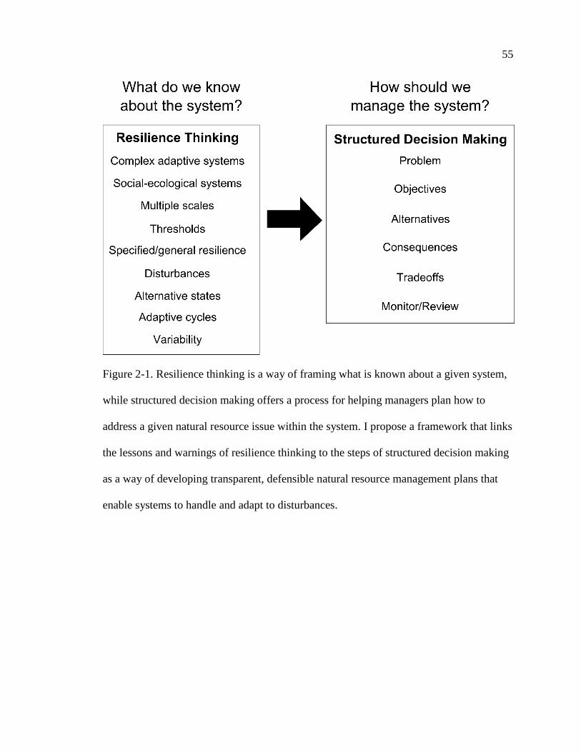
55
Figure 2-1. Resilience thinking is a way of framing what is known about a given system,
while structured decision making offers a process for helping managers plan how to
address a given natural resource issue within the system. I propose a framework that links
the lessons and warnings of resilience thinking to the steps of structured decision making
as a way of developing transparent, defensible natural resource management plans that
enable systems to handle and adapt to disturbances.

Figure 2-2. Spiderweb diagrams offer a way of graphically representing consequences for
constructed performance measures based on properties of resilience. This method allows
for visual comparisons of alternatives in the context of general resilience, which can aid
in the assessment of tradeoffs. For example, decision makers can look at the area covered
and where peaks and valleys occur between alternatives. The diagrams above show the
hypothetical general resilience-related consequences for two alternatives (A and B).
Alternative B is more evenly spread and appears to cover more area, but there are places
where alternative A outperforms alternative B, such as for ecological variability and

57
innovation. Both alternatives have extreme high and low points, which may be
concerning depending on how strongly these performance measures are weighted by the
decision maker(s).
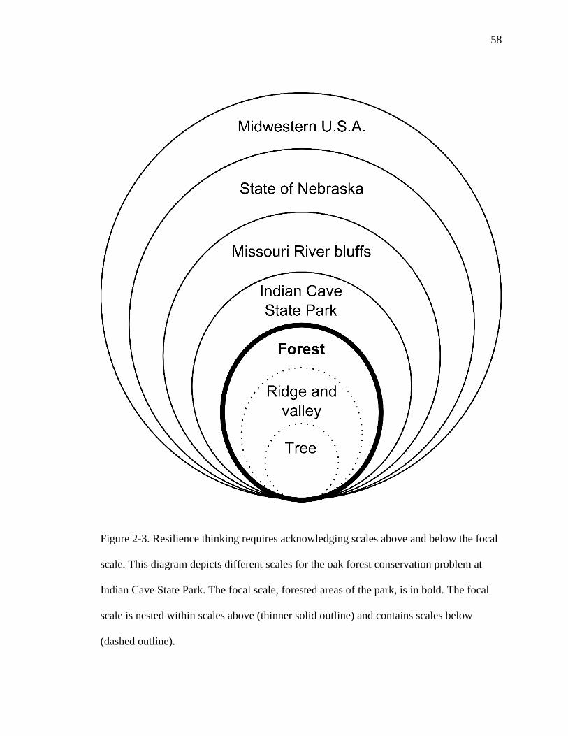
58
Figure 2-3. Resilience thinking requires acknowledging scales above and below the focal
scale. This diagram depicts different scales for the oak forest conservation problem at
Indian Cave State Park. The focal scale, forested areas of the park, is in bold. The focal
scale is nested within scales above (thinner solid outline) and contains scales below
(dashed outline).

59
Figure 2-4. Ball-and-cup diagram of two alternative stable states (oak-attracted, shady-
attracted) for the forest system at Indian Cave State Park. Within the alternatives states,
the system can be (a) oak-dominated and recently burned, (b) oak-dominated and not
recently burned, (c) mixed oak and shade tree, or (d) shady. In the absence of fire, all else
being equal, the system is predicted to move from the oak-attracted state to the shady-
attracted state. The system exhibits hysteresis, such that it takes more effort to cross back
over the threshold from the shady-attracted state to the oak-attracted state than it does to
go from oak-attracted to shady-attracted; this is indicated by the deeper “cup” for the
shady-attracted state than the oak-attracted state.
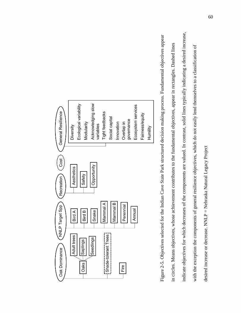
60
Fig
ure
2-5
. O
bje
ctiv
es s
elec
ted f
or
the
India
n C
ave
Sta
te P
ark s
truct
ure
d d
ecis
ion m
akin
g p
roce
ss. F
undam
enta
l obje
ctiv
es a
ppea
r
in c
ircl
es. M
eans
obje
ctiv
es, w
hose
ach
ievem
ent
contr
ibute
s to
the
fundam
enta
l obje
ctiv
es, ap
pea
r in
rec
tan
gle
s. D
ashed
lin
es
indic
ate
obje
ctiv
es f
or
whic
h d
ecre
ases
of
the
com
ponen
ts a
re v
alu
ed.
In c
ontr
ast,
soli
d l
ines
typic
ally
indic
atin
g a
des
ired
incr
ease
,
wit
h t
he
exce
pti
on t
he
com
ponen
ts o
f gen
eral
res
ilie
nce
obje
ctiv
es, w
hic
h d
o n
ot
easi
ly l
end t
hem
selv
es t
o a
cla
ssif
icat
ion o
f
des
ired
incr
ease
or
dec
reas
e. N
NL
P =
Neb
rask
a N
atura
l L
egac
y P
roje
ct
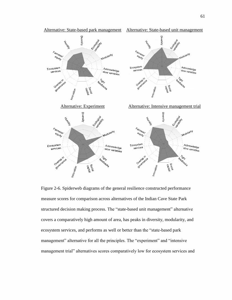
61
Alternative: State-based park management Alternative: State-based unit management
Alternative: Experiment Alternative: Intensive management trial
Figure 2-6. Spiderweb diagrams of the general resilience constructed performance
measure scores for comparison across alternatives of the Indian Cave State Park
structured decision making process. The “state-based unit management” alternative
covers a comparatively high amount of area, has peaks in diversity, modularity, and
ecosystem services, and performs as well or better than the “state-based park
management” alternative for all the principles. The “experiment” and “intensive
management trial” alternatives scores comparatively low for ecosystem services and

62
ecological variability, but receives higher scores for humility and innovation than the
“state-based unit management” alternative.
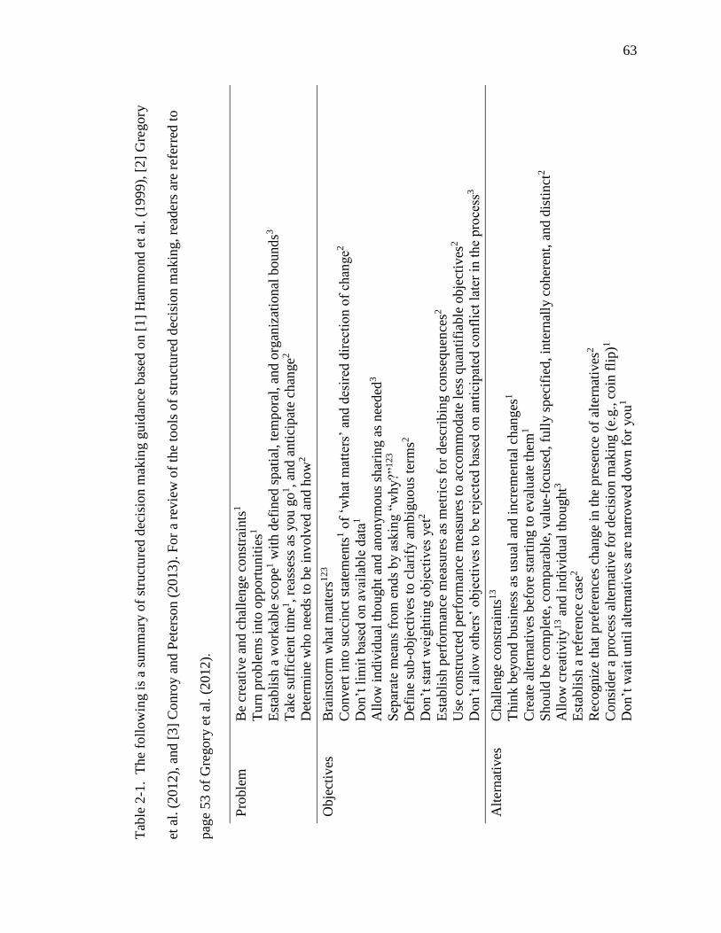
63
Tab
le 2
-1. T
he
foll
ow
ing i
s a
sum
mar
y o
f st
ruct
ure
d d
ecis
ion m
akin
g g
uid
ance
bas
ed o
n [
1]
Ham
mond e
t al
. (1
999),
[2]
Gre
gory
et a
l. (
2012
), a
nd [
3]
Conro
y a
nd P
eter
son (
2013
). F
or
a re
vie
w o
f th
e to
ols
of
stru
cture
d d
ecis
ion m
akin
g, re
ader
s ar
e re
ferr
ed t
o
pag
e 5
3 o
f G
regory
et
al.
(2012).
Pro
ble
m
Be
crea
tive
and c
hal
len
ge
const
rain
ts1
Turn
pro
ble
ms
into
opport
unit
ies1
Est
abli
sh a
work
able
sco
pe1
wit
h d
efin
ed s
pat
ial,
tem
pora
l, a
nd o
rgan
izat
ional
bounds3
Tak
e su
ffic
ient
tim
e1, re
asse
ss a
s you g
o1, an
d a
nti
cipat
e ch
ange2
Det
erm
ine
who n
eeds
to b
e in
volv
ed a
nd h
ow
2
Obje
ctiv
es
Bra
inst
orm
wh
at m
atte
rs1
23
Conver
t in
to s
ucc
inct
sta
tem
ents
1 o
f ‘w
hat
mat
ters
’ an
d d
esir
ed d
irec
tion o
f ch
ange2
Don’t
lim
it b
ased
on a
vai
lable
dat
a1
All
ow
indiv
idual
thought
and a
no
nym
ous
shar
ing a
s nee
ded
3
Sep
arat
e m
eans
from
end
s b
y a
skin
g “
wh
y?”1
23
Def
ine
sub
-obje
ctiv
es t
o c
lari
fy a
mbig
uous
term
s2
Don’t
sta
rt w
eighti
ng o
bje
ctiv
es y
et2
Est
abli
sh p
erfo
rman
ce m
easu
res
as m
etri
cs f
or
des
crib
ing c
onse
quen
ces2
Use
const
ruct
ed p
erfo
rman
ce m
easu
res
to a
ccom
modat
e le
ss q
uan
tifi
able
obje
ctiv
es2
Don’t
all
ow
oth
ers’
obje
ctiv
es t
o b
e re
ject
ed b
ased
on a
nti
cipat
ed c
onfl
ict
late
r in
th
e p
roce
ss3
Alt
ernat
ives
C
hal
lenge
const
rain
ts1
3
Thin
k b
eyond b
usi
nes
s as
usu
al a
nd i
ncr
emen
tal
chan
ges
1
Cre
ate
alte
rnat
ives
bef
ore
sta
rtin
g t
o e
val
uat
e th
em1
Should
be
com
ple
te, co
mpar
able
, v
alue-
focu
sed, fu
lly s
pec
ifie
d, in
tern
ally
coher
ent,
and d
isti
nct
2
All
ow
cre
ativ
ity
13 a
nd i
ndiv
idual
thought3
Est
abli
sh a
ref
eren
ce c
ase2
Rec
ogniz
e th
at p
refe
rence
s ch
ange
in t
he
pre
sen
ce o
f al
tern
ativ
es2
Consi
der
a p
roce
ss a
lter
nat
ive
for
dec
isio
n m
akin
g (
e.g.,
coin
fli
p)1
Don’t
wai
t unti
l al
tern
ativ
es a
re n
arro
wed
dow
n f
or
you
1
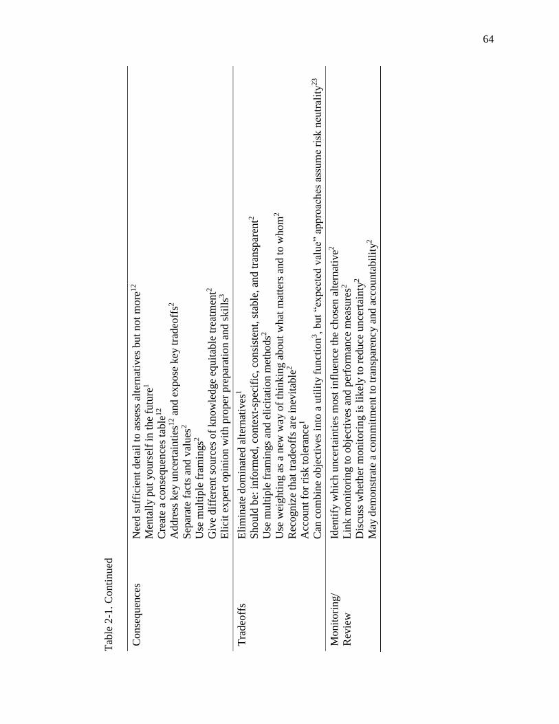
64
Tab
le 2
-1. C
onti
nued
Conse
quen
ces
Nee
d s
uff
icie
nt
det
ail
to a
sses
s al
tern
ativ
es b
ut
no
t m
ore
12
Men
tall
y p
ut
yours
elf
in t
he
futu
re1
Cre
ate
a co
nse
quen
ces
table
12
Addre
ss k
ey u
nce
rtai
nti
es1
2 a
nd e
xpose
key
tra
deo
ffs2
Sep
arat
e fa
cts
and v
alues
2
Use
mult
iple
fra
min
gs2
Giv
e dif
fere
nt
sou
rces
of
know
ledge
equit
able
tre
atm
ent2
Eli
cit
exper
t opin
ion w
ith p
roper
pre
par
atio
n a
nd s
kil
ls3
Tra
deo
ffs
Eli
min
ate
dom
inat
ed a
lter
nat
ives
1
Should
be:
info
rmed
, co
nte
xt-
spec
ific
, co
nsi
sten
t, s
table
, an
d t
ransp
aren
t2
Use
mult
iple
fra
min
gs
and e
lici
tati
on m
ethods2
Use
wei
ghti
ng a
s a
new
way o
f th
inkin
g a
bout
what
mat
ters
and t
o w
hom
2
Rec
ogniz
e th
at t
radeo
ffs
are
inev
itab
le2
Acc
ount
for
risk
tole
rance
1
Can
com
bin
e obje
ctiv
es i
nto
a u
tili
ty f
un
ctio
n3, but
“ex
pec
ted v
alue”
appro
aches
ass
um
e ri
sk n
eutr
alit
y2
3
Monit
ori
ng/
Rev
iew
Iden
tify
whic
h u
nce
rtai
nti
es m
ost
infl
uen
ce t
he
chose
n a
lter
nat
ive2
Lin
k m
onit
ori
ng t
o o
bje
ctiv
es a
nd p
erfo
rman
ce m
easu
res2
Dis
cuss
wh
ether
monit
ori
ng i
s li
kel
y t
o r
educe
un
cert
ainty
2
May
dem
on
stra
te a
com
mit
men
t to
tra
nsp
aren
cy a
nd a
ccounta
bil
ity
2
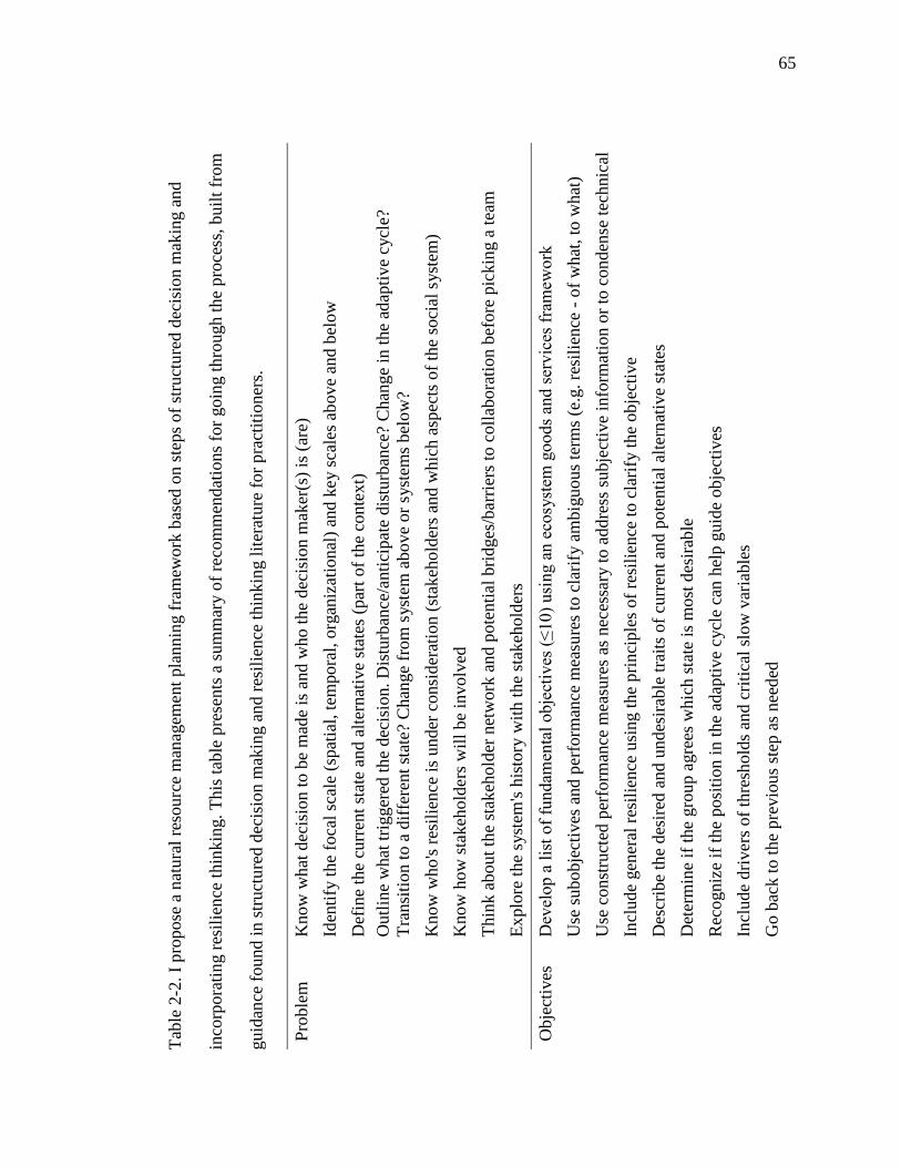
65
Tab
le 2
-2.
I p
ropose
a n
atura
l re
sourc
e m
anag
emen
t pla
nnin
g f
ram
ework
bas
ed o
n s
teps
of
stru
ctu
red d
ecis
ion m
akin
g a
nd
inco
rpora
tin
g r
esil
ien
ce t
hin
kin
g. T
his
tab
le p
rese
nts
a s
um
mar
y o
f re
com
men
dat
ions
for
goin
g t
hro
ugh t
he
pro
cess
, buil
t fr
om
gu
idan
ce f
ound i
n s
truct
ure
d d
ecis
ion
mak
ing a
nd r
esil
ience
thin
kin
g l
iter
ature
for
pra
ctit
ion
ers.
Pro
ble
m
Know
what
dec
isio
n t
o b
e m
ade
is a
nd w
ho t
he
dec
isio
n m
aker
(s)
is (
are)
Id
enti
fy t
he
foca
l sc
ale
(spat
ial,
tem
pora
l, o
rgan
izat
ional
) an
d k
ey s
cale
s ab
ove
and b
elow
D
efin
e th
e cu
rren
t st
ate
and a
lter
nat
ive
stat
es (
par
t of
the
conte
xt)
Outl
ine
what
tri
gger
ed t
he
dec
isio
n. D
istu
rban
ce/a
nti
cipat
e dis
turb
ance
? C
han
ge
in t
he
adap
tive
cycl
e?
Tra
nsi
tion t
o a
dif
fere
nt
stat
e? C
han
ge
from
syst
em a
bove
or
syst
ems
bel
ow
?
K
now
who
's r
esil
ience
is
und
er c
onsi
der
atio
n (
stak
ehold
ers
and w
hic
h a
spec
ts o
f th
e so
cial
syst
em)
K
now
how
sta
keh
old
ers
wil
l be
involv
ed
T
hin
k a
bout
the
stak
ehold
er n
etw
ork
and p
ote
nti
al b
ridges
/bar
rier
s to
coll
abora
tion b
efore
pic
kin
g a
tea
m
E
xplo
re t
he
syst
em's
his
tory
wit
h t
he
stak
ehold
ers
Obje
ctiv
es
Dev
elop a
lis
t of
fund
amen
tal
obje
ctiv
es (
≤10)
usi
ng a
n e
cosy
stem
goods
and s
ervic
es f
ram
ework
U
se s
ubobje
ctiv
es a
nd p
erfo
rman
ce m
easu
res
to c
lari
fy a
mbig
uous
term
s (e
.g. re
sili
ence
- o
f w
hat
, to
what
)
U
se c
onst
ruct
ed p
erfo
rman
ce m
easu
res
as n
eces
sary
to a
dd
ress
sub
ject
ive
info
rmat
ion o
r to
conden
se t
echnic
al
In
clude
gen
eral
res
ilie
nce
usi
ng t
he
pri
nci
ple
s of
resi
lien
ce t
o c
lari
fy t
he
ob
ject
ive
D
escr
ibe
the
des
ired
and u
ndes
irab
le t
rait
s of
curr
ent
and p
ote
nti
al a
lter
nat
ive
stat
es
D
eter
min
e if
the
gro
up a
gre
es w
hic
h s
tate
is
most
des
irab
le
R
ecogniz
e if
the
posi
tion
in t
he
adap
tive
cycl
e ca
n h
elp g
uid
e obje
ctiv
es
In
clude
dri
ver
s of
thre
shold
s an
d c
riti
cal
slow
var
iable
s
G
o b
ack t
o t
he
pre
vio
us
step
as
nee
ded

66
Tab
le 2
-2. C
onti
nued
Alt
ern
ativ
es
Consi
der
non-s
tati
c st
rate
gie
s th
at e
ither
em
bra
ce s
tate
-bas
ed v
aria
bil
ity o
r in
ten
tional
ly i
ntr
od
uce
var
iab
ilit
y
In
clude
man
ipula
tion o
f dis
turb
ance
s or
dis
turb
ance
res
ponse
Know
what
alt
ernat
ives
are
avai
lable
giv
en t
he
curr
ent
posi
tion i
n t
he
adap
tive
cycl
e at
the
foca
l sc
ale
and s
cale
s
bel
ow
and a
bov
e
Id
enti
fy a
lter
nat
ives
that
man
ipula
te p
osi
tion r
elat
ive
to a
thre
shold
, or
that
move
a th
resh
old
its
elf
C
onsi
der
chan
gin
g o
r in
stit
uti
ng r
ule
s an
d h
ow
they
are
en
forc
ed
G
o b
ack t
o p
revio
us
step
s as
nee
ded
Co
nse
qu
ence
s R
epre
sent
unce
rtai
nty
, w
hic
h m
ay i
ncl
ude
par
tial
contr
oll
abil
ity b
ased
on r
ule
en
forc
emen
t
U
se m
odel
s to
conce
ptu
aliz
e sy
stem
com
ponen
ts a
nd d
yn
amic
s
C
onsi
der
infl
uen
ce f
rom
oth
er s
cale
s o
r on o
ther
sca
les,
incl
udin
g h
ow
thre
shold
s at
oth
er s
cale
s
Id
enti
fy a
ssum
pti
ons
acro
ss e
xper
ts a
nd p
arti
cipan
ts
U
se p
ast
dis
turb
ance
his
tory
to h
elp p
redic
t fu
ture
res
ponse
s
In
clude
pro
bab
ilit
ies
of
flip
pin
g i
nto
an a
lter
nat
ive
stat
e, c
onsi
der
ing k
now
n o
r an
tici
pat
ed t
hre
shold
s
D
iscu
ss t
he
anti
cipat
ed r
ever
sibil
ity o
f a
flip
Id
enti
fy h
ow
an a
lter
nat
ive
infl
uen
ces
syst
em d
riv
ers,
incl
udin
g c
riti
cal
slo
w v
aria
ble
s
C
onsi
der
what
the
tran
siti
on w
ould
be
like
(not
just
the
end s
tate
)
T
hin
k a
bout
how
an a
lter
nat
ive
may i
nfl
uen
ce t
ren
ds
in p
roper
ties
of
gen
eral
res
ilie
nce
(e.
g., d
iver
sity
)
G
o b
ack t
o p
revio
us
step
s as
nee
ded

67
Tab
le 2
-2. C
onti
nued
Tra
deo
ffs
Eli
min
ate
obje
ctiv
es t
hat
do n
ot
hel
p d
isti
nguis
h b
etw
een a
lter
nat
ives
to s
imply
K
now
the
trad
eoff
s bet
wee
n e
cosy
stem
ser
vic
es a
nd b
etw
een a
lter
nat
ive
stat
es
U
nder
stan
d t
he
pote
nti
al r
isks,
par
ticu
larl
y r
elat
ed t
o s
ud
den
tra
nsi
tions
R
ecogniz
e th
e ri
sk t
ole
rance
of
dec
isio
n m
aker
s
C
onsi
der
how
ch
angin
g o
ne
thre
shold
or
posi
tion r
elat
ive
to a
thre
shold
may
infl
uen
ce o
ther
thre
sho
lds
G
o b
ack t
o p
revio
us
step
s as
nee
ded
Monit
ori
ng/
Look f
or
tren
ds,
in t
erm
s of
quan
titi
es a
nd r
ates
(e.
g., i
ncr
easi
ng v
aria
bil
ity)
Rev
iew
F
oll
ow
both
fas
t an
d s
low
var
iable
s (e
ven
if
they w
ere
elim
inat
ed a
s obje
ctiv
es d
uri
ng t
he
trad
eoff
s st
ep)
C
onsi
der
how
key u
nce
rtai
nti
es m
ight
be
reduce
d t
hro
ugh t
hou
ghtf
ul
monit
ori
ng a
nd
anal
ysi
s
L
ook f
or
chan
ges
in a
ttit
udes
/val
ues
G
o b
ack t
o p
revio
us
step
s as
nee
ded
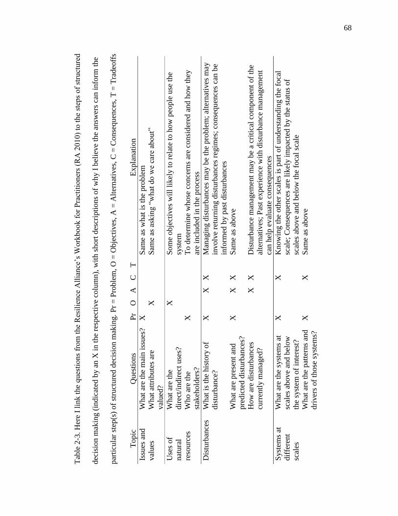
68
Tab
le 2
-3. H
ere
I li
nk t
he
ques
tions
from
the
Res
ilie
nce
All
iance
’s W
ork
bo
ok f
or
Pra
ctit
ioner
s (R
A 2
010)
to t
he
step
s of
stru
cture
d
dec
isio
n m
akin
g (
indic
ated
by a
n X
in t
he
resp
ecti
ve
colu
mn),
wit
h s
hort
des
crip
tio
ns
of
wh
y I
bel
ieve
the
answ
ers
can i
nfo
rm t
he
par
ticu
lar
step
(s)
of
stru
cture
d d
ecis
ion m
akin
g.
Pr
= P
roble
m,
O =
Obje
ctiv
es,
A =
Alt
ern
ativ
es, C
= C
on
seq
uen
ces,
T =
Tra
deo
ffs
Topic
Q
ues
tions
Pr
O
A
C
T
Ex
pla
nat
ion
Issu
es a
nd
val
ues
What
are
the
mai
n i
ssues
?
X
Sam
e as
what
is
the
pro
ble
m
What
att
ribute
s ar
e
val
ued
?
X
Sam
e as
ask
ing “
wh
at d
o w
e ca
re a
bout”
Use
s of
nat
ura
l
reso
urc
es
What
are
the
dir
ect/
indir
ect
use
s?
X
Som
e obje
ctiv
es w
ill
lik
ely t
o r
elat
e to
how
peo
ple
use
the
syst
em
Who a
re t
he
stak
ehold
ers?
X
To d
eter
min
e w
hose
co
nce
rns
are
con
sid
ered
an
d h
ow
th
ey
are
incl
uded
in t
he
pro
cess
Dis
turb
ance
s W
hat
is
the
his
tory
of
dis
turb
ance
?
X
X
X
Man
agin
g d
istu
rban
ces
may
be
the
pro
ble
m;
alte
rnat
ives
may
involv
e re
turn
ing d
istu
rban
ces
regim
es;
conse
qu
ence
s ca
n b
e
info
rmed
by p
ast
dis
turb
ance
s
What
are
pre
sent
and
pre
dic
ted d
istu
rban
ces?
X
X
X
Sam
e as
above
How
are
dis
turb
ance
s
curr
entl
y m
anag
ed?
X
X
D
istu
rban
ce m
anag
emen
t m
ay b
e a
crit
ical
com
po
nen
t of
the
alte
rnat
ives
; P
ast
exper
ience
wit
h d
istu
rban
ce m
anag
emen
t
can h
elp e
val
uat
e co
nse
quen
ces
Syst
ems
at
dif
fere
nt
scal
es
What
are
the
syst
ems
at
scal
es a
bov
e an
d b
elow
the
syst
em o
f in
tere
st?
X
X
K
now
ing t
he
oth
er s
cale
s is
par
t of
under
stan
din
g t
he
foca
l
scal
e; C
onse
quen
ces
are
likel
y i
mpac
ted b
y t
he
stat
us
of
scal
es a
bov
e an
d b
elow
the
foca
l sc
ale
What
are
the
pat
tern
s an
d
dri
ver
s of
those
syst
ems?
X
X
S
ame
as a
bove
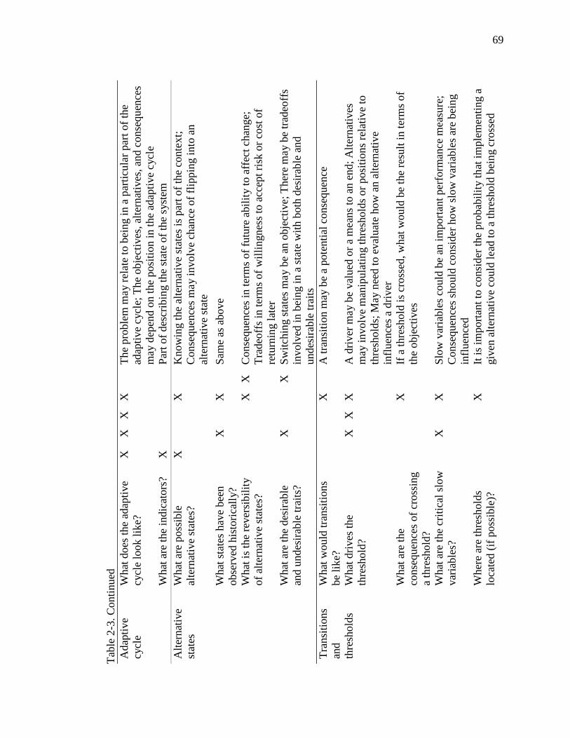
69
Tab
le 2
-3. C
onti
nued
Adap
tive
cycl
e
What
does
the
adap
tive
cycl
e lo
ok l
ike?
X
X
X
X
T
he
pro
ble
m m
ay r
elat
e to
bei
ng i
n a
par
ticu
lar
par
t of
the
adap
tive
cycl
e; T
he
obje
ctiv
es, al
tern
ativ
es,
and c
onse
quen
ces
may
dep
end o
n t
he
posi
tion i
n t
he
adap
tive
cycl
e
What
are
the
indic
ators
?
X
Par
t of
des
crib
ing t
he
stat
e o
f th
e sy
stem
Alt
ernat
ive
stat
es
What
are
poss
ible
alte
rnat
ive
stat
es?
X
X
K
now
ing t
he
alte
rnat
ive
stat
es i
s par
t of
the
conte
xt;
Conse
quen
ces
may i
nvolv
e ch
ance
of
flip
pin
g i
nto
an
alte
rnat
ive
stat
e
What
sta
tes
hav
e bee
n
obse
rved
his
tori
call
y?
X
X
S
ame
as a
bove
What
is
the
rever
sibil
ity
of
alte
rnat
ive
stat
es?
X
X
C
onse
quen
ces
in t
erm
s o
f fu
ture
abil
ity t
o a
ffec
t ch
ange;
Tra
deo
ffs
in t
erm
s of
wil
lingnes
s to
acc
ept
risk
or
cost
of
retu
rnin
g l
ater
What
are
the
des
irab
le
and u
ndes
irab
le t
rait
s?
X
X
S
wit
chin
g s
tate
s m
ay b
e an
obje
ctiv
e; T
her
e m
ay b
e tr
adeo
ffs
involv
ed i
n b
eing i
n a
sta
te w
ith b
oth
des
irab
le a
nd
undes
irab
le t
rait
s
Tra
nsi
tio
ns
and
thre
shold
s
What
would
tra
nsi
tions
be
like?
X
A t
ransi
tion m
ay b
e a
pote
nti
al c
onse
quen
ce
What
dri
ves
the
thre
shold
?
X
X
X
A d
river
may b
e val
ued
or
a m
eans
to a
n e
nd;
Alt
ernat
ives
may
involv
e m
anip
ula
tin
g t
hre
shold
s or
posi
tions
rela
tive
to
thre
shold
s; M
ay n
eed t
o e
val
uat
e h
ow
an
alt
ern
ativ
e
infl
uen
ces
a d
river
What
are
the
conse
quen
ces
of
cross
ing
a th
resh
old
?
X
If a
thre
shold
is
cross
ed,
what
would
be
the
resu
lt i
n t
erm
s of
the
obje
ctiv
es
What
are
the
crit
ical
slo
w
var
iable
s?
X
X
S
low
var
iable
s co
uld
be
an i
mport
ant
per
form
ance
mea
sure
;
Conse
quen
ces
should
co
nsi
der
how
slo
w v
aria
ble
s ar
e bei
ng
infl
uen
ced
Wher
e ar
e th
resh
old
s
loca
ted (
if p
oss
ible
)?
X
It i
s im
port
ant
to c
onsi
der
the
pro
bab
ilit
y t
hat
im
ple
men
ting a
giv
en a
lter
nat
ive
could
lea
d t
o a
thre
shold
bei
ng c
ross
ed
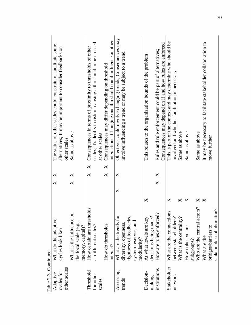
70
Tab
le 2
-3. C
onti
nued
Adap
tive
cycl
es f
or
oth
er s
cale
s
What
do t
he
adap
tive
cycl
es l
ook l
ike?
X
X
T
he
stat
us
of
oth
er s
cale
s co
uld
const
rain
or
faci
lita
te s
om
e
alte
rnat
ives
; It
may b
e im
port
ant
to c
onsi
der
fee
db
acks
on
oth
er s
cale
s
What
is
the
infl
uen
ce o
n
the
foca
l sc
ale
(e.g
.,
mem
ory
, ca
pit
al)?
X
X
S
ame
as a
bove
Thre
shold
for
oth
er
scal
es
How
cer
tain
are
thre
shold
s
at d
iffe
rent
scal
es?
X
X
C
onse
quen
ces
in t
erm
s o
f pro
xim
ity t
o t
hre
shold
s of
oth
er
scal
es;
Tra
deo
ffs
in r
isk o
f ca
usi
ng a
thre
shold
to b
e cr
oss
ed
at o
ther
sca
les
How
do t
hre
shold
s
inte
ract
?
X
X
C
onse
quen
ces
may d
iffe
r dep
endin
g o
n t
hre
shold
inte
ract
ions;
Chan
gin
g o
ne
thre
shold
could
infl
uen
ce a
noth
er
Ass
essi
ng
tren
ds
What
are
the
tren
ds
for
div
ersi
ty, open
nes
s,
tightn
ess
of
feed
bac
ks,
syst
em r
eser
ves
, an
d
modula
rity
?
X
X
O
bje
ctiv
es c
ould
involv
e ch
angin
g t
ren
ds;
Co
nse
qu
ence
s m
ay
involv
e in
fluen
cing a
tre
nd o
r m
ay b
e su
bje
ct t
o a
tre
nd
Dec
isio
n-
mak
ing
inst
ituti
on
s
At
what
lev
els
are
key
dec
isio
ns
bei
ng m
ade?
X
This
rel
ates
to t
he
org
aniz
atio
n b
ounds
of
the
pro
ble
m
How
are
rule
s en
forc
ed?
X
X
R
ule
s an
d r
ule
enfo
rcem
ent
could
be
par
t o
f al
tern
ativ
es;
Conse
quen
ces
may d
epen
d o
n i
f an
d h
ow
rule
s ar
e en
forc
ed
Sta
keh
old
er
net
work
What
are
the
conn
ecti
ons
bet
wee
n s
tak
ehold
ers?
X
This
is
par
t of
the
conte
xt
and m
ay d
eter
min
e w
ho
should
be
involv
ed a
nd w
het
her
fac
ilit
atio
n i
s nec
essa
ry
What
is
the
centr
alit
y?
X
Sam
e as
above
How
cohes
ive
are
subgro
ups?
X
Sam
e as
above
Who a
re t
he
centr
al a
cto
rs?
X
Sam
e as
above
What
are
the
bri
dges
/bar
rier
s to
stak
ehold
er c
oll
abo
rati
on
?
X
It m
ay b
e nec
essa
ry t
o f
acil
itat
e st
akeh
old
er c
oll
abora
tion t
o
move
furt
her
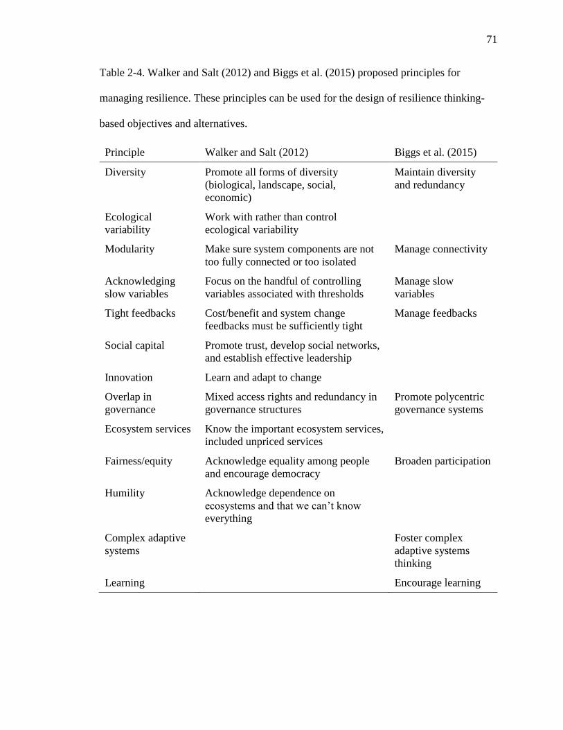
71
Table 2-4. Walker and Salt (2012) and Biggs et al. (2015) proposed principles for
managing resilience. These principles can be used for the design of resilience thinking-
based objectives and alternatives.
Principle Walker and Salt (2012) Biggs et al. (2015)
Diversity Promote all forms of diversity
(biological, landscape, social,
economic)
Maintain diversity
and redundancy
Ecological
variability
Work with rather than control
ecological variability
Modularity Make sure system components are not
too fully connected or too isolated
Manage connectivity
Acknowledging
slow variables
Focus on the handful of controlling
variables associated with thresholds
Manage slow
variables
Tight feedbacks Cost/benefit and system change
feedbacks must be sufficiently tight
Manage feedbacks
Social capital Promote trust, develop social networks,
and establish effective leadership
Innovation Learn and adapt to change
Overlap in
governance
Mixed access rights and redundancy in
governance structures
Promote polycentric
governance systems
Ecosystem services Know the important ecosystem services,
included unpriced services
Fairness/equity Acknowledge equality among people
and encourage democracy
Broaden participation
Humility Acknowledge dependence on
ecosystems and that we can’t know
everything
Complex adaptive
systems
Foster complex
adaptive systems
thinking
Learning Encourage learning
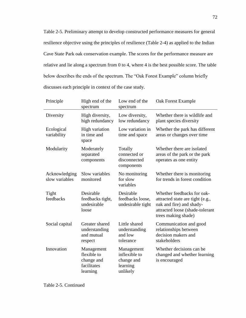
72
Table 2-5. Preliminary attempt to develop constructed performance measures for general
resilience objective using the principles of resilience (Table 2-4) as applied to the Indian
Cave State Park oak conservation example. The scores for the performance measure are
relative and lie along a spectrum from 0 to 4, where 4 is the best possible score. The table
below describes the ends of the spectrum. The “Oak Forest Example” column briefly
discusses each principle in context of the case study.
Principle High end of the
spectrum
Low end of the
spectrum
Oak Forest Example
Diversity High diversity,
high redundancy
Low diversity,
low redundancy
Whether there is wildlife and
plant species diversity
Ecological
variability
High variation
in time and
space
Low variation in
time and space
Whether the park has different
areas or changes over time
Modularity Moderately
separated
components
Totally
connected or
disconnected
components
Whether there are isolated
areas of the park or the park
operates as one entity
Acknowledging
slow variables
Slow variables
monitored
No monitoring
for slow
variables
Whether there is monitoring
for trends in forest condition
Tight
feedbacks
Desirable
feedbacks tight,
undesirable
loose
Desirable
feedbacks loose,
undesirable tight
Whether feedbacks for oak-
attracted state are tight (e.g.,
oak and fire) and shady-
attracted loose (shade-tolerant
trees making shade)
Social capital Greater shared
understanding
and mutual
respect
Little shared
understanding
and low
tolerance
Communication and good
relationships between
decision makers and
stakeholders
Innovation Management
flexible to
change and
facilitates
learning
Management
inflexible to
change and
learning
unlikely
Whether decisions can be
changed and whether learning
is encouraged
Table 2-5. Continued

73
Overlap in
governance
Management
across scales
and with
different
decision
processes
Management all
at one scale with
one decision
process
Whether management of the
oak forest, within and
surrounding the park, are
addressed by multiple groups
Ecosystem
services
High levels and
diversity of
services
Low levels and
diversity of
services
How well the park provides
the ecosystem services valued
by the various stakeholders
Fairness/equity Decisions
perceived as fair
Decisions
perceived as
unfair
Whether stakeholders are
satisfied with how
management decisions are
made and implemented
Humility Recognizes
limits to
predictability
Assumes near
perfect
predictability
Whether uncertainty is
addressed or ignored
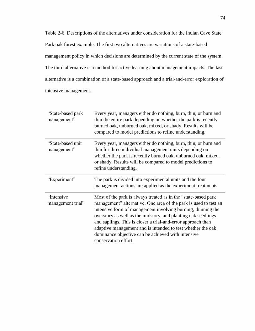
74
Table 2-6. Descriptions of the alternatives under consideration for the Indian Cave State
Park oak forest example. The first two alternatives are variations of a state-based
management policy in which decisions are determined by the current state of the system.
The third alternative is a method for active learning about management impacts. The last
alternative is a combination of a state-based approach and a trial-and-error exploration of
intensive management.
“State-based park
management”
Every year, managers either do nothing, burn, thin, or burn and
thin the entire park depending on whether the park is recently
burned oak, unburned oak, mixed, or shady. Results will be
compared to model predictions to refine understanding.
“State-based unit
management”
Every year, managers either do nothing, burn, thin, or burn and
thin for three individual management units depending on
whether the park is recently burned oak, unburned oak, mixed,
or shady. Results will be compared to model predictions to
refine understanding.
“Experiment” The park is divided into experimental units and the four
management actions are applied as the experiment treatments.
“Intensive
management trial”
Most of the park is always treated as in the “state-based park
management” alternative. One area of the park is used to test an
intensive form of management involving burning, thinning the
overstory as well as the midstory, and planting oak seedlings
and saplings. This is closer a trial-and-error approach than
adaptive management and is intended to test whether the oak
dominance objective can be achieved with intensive
conservation effort.
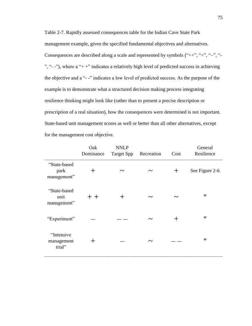
75
Table 2-7. Rapidly assessed consequences table for the Indian Cave State Park
management example, given the specified fundamental objectives and alternatives.
Consequences are described along a scale and represented by symbols (“++”, “+”, “~”, “-
”, “- -”), where a “+ +” indicates a relatively high level of predicted success in achieving
the objective and a “- -” indicates a low level of predicted success. As the purpose of the
example is to demonstrate what a structured decision making process integrating
resilience thinking might look like (rather than to present a precise description or
prescription of a real situation), how the consequences were determined is not important.
State-based unit management scores as well or better than all other alternatives, except
for the management cost objective.
Oak
Dominance
NNLP
Target Spp Recreation Cost
General
Resilience
“State-based
park
management” + ~ ~ + See Figure 2-6
“State-based
unit
management” + + + ~ ~ ″
“Experiment” – – – ~ + ″
“Intensive
management
trial” + – ~ – – ″
76
8 APPENDIX: Suggested readings
Resilience Alliance (RA). 2010. Assessing resilience in social-ecological systems:
Workbook for practitioners. Version 2.0. Online: http://www.resalliance.org/3871.php
Assessing Resilience in Social-Ecological Systems: Workbook for Practitioners,
Revised Version 2.0 is a product of the Resilience Alliance “designed to assist in
resolving specific resource issues and in developing and implementing management goals
without compromising the resilience and integrity of the system as a whole.” A major
component of the assessment is answering a set of questions related to the social
ecological system of interest in an effort to characterize its resilience. These questions
have been summarized in Table 2.
Biggs, R., M. Schlüter, and M. Schoon (eds). 2015. Principles for building resilience:
sustaining ecosystem services in social-ecological systems. Cambridge University Press,
Cambridge, UK.
This is a short book presenting principles for building resilience, along with
examples and key points for implementation. Biggs et al. (2012) contains similar
information, presented in a journal article format. The Stockholm Resilience Centre
released a pamphlet summarizing the book, “Applying resilience thinking: seven
principles for building resilience in social-ecological systems,” which is available online:
http://www.stockholmresilience.org/21/research/research-news/4-22-2014-applying-
resilience-thinking.html

77
Walker, B. H., and D. Salt. 2006. Resilience thinking: sustaining ecosystems and people
in a changing world. Island Press, Washington, D.C.
Walker, B., and D. Salt. 2012. Resilience thinking: sustaining ecosystems and people in a
changing world. Island Press, Washington, D.C.
Resilience Thinking (2006) and Resilience Practice (2012) are a sequence of short
books by Walker and Salt that describe the main tenets of resilience science and present
suggestions about how resilience-based management may be implemented in simple,
understandable language. Book reviews and personal experience indicate that these books
are a great starting place for exposing practitioners to resilience concepts in an easily
accessible format.
Conroy, M. J., and Peterson, J. T. 2013. Decision making in natural resource
management: A structured, adaptive approach. John Wiley & Sons, Chichester, West
Sussex, UK.
This textbook by M. Conroy and J. Peterson is intended for scientists, managers,
and students interested in applying a structured approach to complex natural resource
issues. It includes descriptions of the components of structured decision making and
detailed discussions on the development of decision models.
Gregory, R., Failing, L., Harstone, M., Long, G., McDaniels, T., and Ohlson, D. 2012.
Structured decision making: a practical guide to environmental management choices.
John Wiley & Sons, Chichester, West Sussex, UK.
78
This textbook by R. Gregory, L. Failing, M. Harstone, G. Long, T. McDaniels,
and D. Ohlson (2012) provides an in-depth description of the structured decision making
process and presents case-study examples. They describe how to defensibly make tough
environmental resource management decisions based on both values and facts.
Hammond, J. S., Keeney, R. L., and Raiffa, H. 1999. Smart choices: a practical guide to
making better life decisions. Broadway Books, New York, New York, USA.
Smart Choices by Hammond, Keeney, and Raiffa (1999) is a short book written to
teach people how to make better life decisions. It has received much attention and been
used by individuals for self-help purposes, by professors in classroom settings, and in
professional training programs (Hammond et al. 1999). The book discussions both what
people do, drawing from psychology, and what people should do. Smart Choices offers
descriptions of the steps of structured decision making in simple, understandable
language.

79
CHAPTER 3: OPTIMIZATION AND RESILIENCE THINKING FOR
MANAGEMENT OF A HYPOTHETICAL MIDWESTERN OAK FOREST
1. INTRODUCTION
Resilience was originally defined in the ecology discipline by C. S. Holling
(1973) as “a measure of the persistence of systems and of their ability to absorb change
and disturbance and still maintain the same relationships between populations or state
variables” (p. 14). Resilience thinking is one of the major drivers behind a shift in natural
resource management toward a complex social-ecological systems paradigm (Millennium
Ecosystem Assessment 2003, Berkes 2010). Key concepts of resilience thinking include:
(a) the potential for alternative stable states and non-linear responses, (b) the importance
of variability and disturbance in maintaining a system state, (c) cross-scale linkages
between/within systems, (d) the presence of emergent properties, and (e) limited
predictability as a result of inherent uncertainty (Walker and Salt 2006). This is in
contrast to traditional steady-state management that sought to reduce variability from an
assumed equilibrium for part of the system (Williams and Brown 2014). Strictly
controlling a system to consistently achieve a given objective may succeed in the short
term but will likely erode resilience and ultimately result in a sudden unexpected
transition (Holling and Meffe 1996, Gunderson 2000).
State-and-transition modeling can conceptually represent a complex system with
alternative stable states and non-linear transitions, and has been suggested as a practical
way of incorporating resilience thinking into management decision making (Westoby et
al. 1989, Bestelmeyer et al. 2004, Briske et al. 2008, Suding and Hobbs 2009, Walker and
80
Salt 2012). In fact, the state-and-transition modeling approach emerged in rangeland
ecology partly in response to the multiple stable states concept of Holling’s (1973)
ecological resilience theory (Briske et al. 2005, Briske et al. 2008). State-and-transition
models were originally designed to frame rangeland management contexts and consisted
of discrete states (described by vegetative composition) and transitions between states
(Westoby et al. 1989). More recent approaches distinguish states, phases within states,
transitions, and thresholds (Stringham et al. 2003).
States are domains of relative stability established through ecological processes.
Phases are recognizable patterns within the bounds of natural variability characteristic of
the state. Transitions are trajectories of change. Thresholds are boundaries between states
for which transitions are irreversible without substantial management input. Additional
modifications, proposed by Briske et al. (2008), further emphasize resilience concepts in
state-and-transition models by explicitly describing triggers, at-risk communities,
feedback mechanisms, restoration pathways, and process-specific indicators. Their
revised state-and-transition model encourages broader inclusion of variables and
processes influencing state resilience and focuses management attention on influencing
proximity to thresholds rather than identifying thresholds (Briske et al. 2008).
The purpose of this chapter is to use a resilience thinking perspective to explore
the potential and limitations of optimizing a state-and-transition model, using a
hypothetical Midwestern oak forest conservation example. Optimization methods,
namely those based on maximum sustainable yield, have been criticized as a primary
cause of past natural resource management catastrophes (e.g., collapsed fisheries,
massive wildlife fires) (Walker and Salt 2006). However, optimization and other decision
81
analysis techniques are not inherently at odds with resilience (Fischer et al. 2009,
Possingham and Biggs 2012, Johnson et al. 2013). When applied as a decision making
tool within a larger resilience-driven management perspective, optimization can identify
policies that are most likely to best achieve the objectives, based on models of values,
consequences, and uncertainty. I use the framework proposed by Briske et al. (2008) to
incorporate resilience concepts into a qualitative state-and-transition model, and then
further apply resilience thinking to quantifying the model for use as a Markov decision
process. Optimal management decisions are identified based on expected value. I briefly
explore uncertainties and tradeoffs and consider how optimization could inform decision
making within a larger resilience thinking paradigm.
2 BACKGROUND
The context of the example is loosely based on experience with an oak forest
system in the Missouri River bluffs of the Midwestern United States. A hypothetical
setting allows for the investigation of management decisions without appearing
prescriptive and provides freedom to manipulate model parameters to make various
points relevant to resilience in the absence of data. In reality, insufficient data can greatly
challenge the applicability of decision analysis tools, making it important to use a
combination of approaches when choosing a management option (Polasky et al. 2011).
The hypothetical oak forest is located on a state park that is managed for
environmental conservation and visitor satisfaction objectives, while also considering
management cost. Historically the area supported oak-dominated forest communities
(Quercus rubra, Q. velutina, Q. macrocarpa, and Q. muehlenbergii) maintained by a

82
relatively frequent fire regime. A general trend of declining oak dominance has been
observed across eastern North America where fire has been excluded (Abrams 1992, Fei
et al. 2011). Managers are concerned that a lack of fire in the park is facilitating a
transition away from an oak forest toward a forest dominated by shade tolerant, less fire-
resistant trees, such as ironwood (Ostrya virginiana). A diversity of flora and fauna live
in the park and have different tolerances and preferences for fire and its impacts on forest
structure, composition, and function.
3 STATE-AND-TRANSITION MODEL AND MANAGEMENT OPTIONS
Following the recommendations of Briske et al. (2008) for developing a state-and-
transition model under a resilience thinking perspective, I explicitly describe triggers, at-
risk communities, feedback mechanisms, and restoration pathways (Figure 3-1). Two
overarching alternative system states have been identified. One state is characterized by a
tendency toward continued oak dominance, and the other is characterized by a tendency
toward dominance by shade tolerant tree species (Nowacki and Abrams 2008). Indicators
of the oak-attracted state include a high number of oak trees and seedlings and a low
density midstory, and indicators of the shady-attracted state include shade-tolerant trees
in the midstory and low light availability in the understory.
The reference state (“oak-attracted”) is maintained by feedbacks encouraging oak
regeneration and discouraging invasion of shade-tolerant trees. For example, oak leaves
would facilitate burning, and burning would lead to conditions favoring oak seedling
survival and ultimately oak regeneration. Fire would suppress shade-tolerant trees that
tend to be less adapted to fire. In contrast, the alternative state (“shady-attracted”) is
83
maintained by feedbacks that suppress oak regeneration by decreasing light availability to
oak seedlings. The threshold between the reference state and the alternative state is
determined by the density of shade-tolerant trees, and decreased frequency of fire can
trigger crossing of the threshold. Once the threshold has been crossed, the only way to
possibly return is to follow the restoration pathway by implementing thinning with or
without burning. Thinning and burning is more likely to reverse the transition. The
system property of being much easier (in terms of management effort) to cross the
threshold into the shady-attracted state than it is to return to the oak-attracted state (which
requires significant management input) is an example of hysteresis (Scheffer and
Carpenter 2003).
Within the oak-attracted state, the system can exist in a recently burned oak
condition or an unburned oak condition. These two conditions are assumed to have
distinguishable community structure, composition, and function but are still within the
same domain. Within the alternative state, the system can be in a mixed condition with
some oaks remaining or in a shady condition without oaks. In the absence of
management, the system will eventually transition to the shady condition. The unburned
oak condition can be thought of as the at-risk community5 phase and may cross the
threshold if triggered by lack of fire.
4 MARKOV DECISION PROCESSES
5 We use the term “community” without specifying what characterized the community beyond presence of
oak and/or shade-tolerant tree species. We assume that there are differences in community composition
between burned and unburned oak forests. (For example, there may be changes in dominant herbaceous
plants.)
84
A Markov decision process is a mathematical model for a time series of discrete
transitions in state with an action taken at each time step, under the assumption that past
conditions do not impact future transitions (Marescot et al. 2013). Components of a
Markov decision process include: (a) possible states and actions, (b) transition
probabilities among states, (c) a reward (i.e. objective, utility) function based on the state
and action taken, and (d) a specified time horizon and discount factor. An overlap in
terminology between state-and-transition models and Markovian decision processes can
lead to confusion (Standish et al. 2008). This overlap is not a coincidence, however, as
both types of models capture the idea of a system being composed of discrete states that
can transition to other states. To reduce ambiguity, in the rest of the chapter, states of the
state-and-transition model (Figure 3-1) are referred to as “conditions” (burned oak
condition, unburned oak condition, mixed condition, shady condition). “States” are either
(a) Markovian states (synonymous with condition for the single unit example and are
counts of units in each condition for the multiple unit example), or (b) alternative stable
states from the resilience thinking perspective (oak-attracted state = burned oak or
unburned oak condition; shady-attracted state = mixed or shady condition). “Transitions”
are movements among Markovian states.
In the following sections, I further specify the Markov decision process described
above and determine the stationary optimal policy6 using MDPSolve (Fackler 2011,
available at https://sites.google.com/site/mdpsolve/) in Matlab (R2011a). I discuss the
time horizon, discount factor, and initially selected transitions probabilities (referred to as
6 A stationary optimal policy dictates the action for each state that is optimal at any time step (i.e., time
independent).

85
the “original”7). I first optimize a simple version of the system, in which the park is
considered a single management unit, for which it is relatively straightforward to
translate the state-and-transition model (Figure 3-1) into a Markovian decision process
model. However, the single unit example does not allow for diversity in condition within
the park for a given time step. As I later discuss, diversity in condition may be desirable
from a resilience thinking perspective. To accommodate different conditions at one time,
I then use a multiple unit example in which the park is divided into three units.
4.1 Time horizon and discount factor
An infinite time horizon and a discount factor of 0.95 were specified for the
Markov decision process. The decision context does not indicate a reason to select a
particular time horizon (e.g., expiration date of a grant). An infinite time horizon was
selected over an arbitrary finite horizon because the optimal decision in the short term
may not be the same as the long term optimal decision (Marescot et al. 2013). Discount
factors can run from 0 to 1, where 0 means future rewards have no value and 1 indicates
rewards received in the future are worth the same as they would be if received in the
present. Given the importance of economic costs and existing social benefits, I felt 0.95
was appropriate for describing the relationship between rewards now and in the future; a
reward in 14 time steps is approximately half of the current reward. However this
discount factor devalues the future more strongly than is sometimes recommended for
long-term planning (e.g., 0.965 for mature European economies (European Union
7 In later sections, the implications of uncertainty about transition probabilities are explored by evaluating
alternatives to the “original.”
86
Regional Policy 2008)). In later sections the discount factor is varied to test the
sensitivity of the optimal policy to the selected discount factor.
4.2 Transition probabilities
Transition probabilities are dependent on which management action is taken
(pij(a)), where actions are a1 = do nothing, a2 = burn, a3 = thin, and a4 = burn and thin.
Initially I assume that transition probabilities are known with certainty. In a later section I
manipulate the transition probabilities to explore the implications of uncertainty;
therefore, I refer to this set of transition matrices as the “original.”
The following basic principles were used in the quantification of transition
probabilities (Figure 3-2, Table 3-1):
In a given time step, a unit may remain in the same state (pii(a)) or
transition once (pij(a)).
In the absence of management intervention (action: a1 = do nothing), there
is a strong tendency to move to the condition immediately to the right
along a pathway from burned oak to unburned oak to mixed to shady (high
probabilities for p12(a1), p23(a1), p34(a1)).
Transitions to a condition more than one step to the right is impossible
(i.e., burned oak cannot transition directly to mixed (p13(a) = 0 ∀ a), and
unburned oak cannot transition directly to shady (p24(a) = 0 ∀ a)).
Transitioning to prior conditions is only possible through management
intervention (p43(a1) = p42(a1) = p41(a1) = p32(a1) = p31(a1) = p21(a1) = 0).
87
Intervention is also needed to remain in the burned oak condition (p11(a1)
= 0).
The shady condition can only move backwards to the mixed condition
(i.e., shady never transitions to unburned oak or burned oak (p42(a) =
p41(a) = 0 ∀ a)).
Certain actions can ensure particular transitions. When managers do nothing (a1)
or thin (a3), burned oak is guaranteed to transition to unburned oak (p12(a1) = p12(a3) = 1)
and shady is guaranteed to stay shady (p44(a1) = p44(a3) = 1). Burning (a2) guarantees that
burned oak remains burned oak (p11(a2) = 1), unburned oak transitions back to burned
oak (p21(a2) = 1), and shady remains shady (p44(a2) = 1). Burning and thinning (a4)
guarantees that burned oak remains burned oak (p11(a4) = 1) and unburned oak transitions
to burned oak (p21(a2) = 1).
All other transitions lie between 0 and 1. In the hypothetical system, fire
disturbance is integral to the dynamics maintaining the oak-attracted state. To represent
this with transition probabilities, in the absence of burning the unburned oak condition
has a strong chance of transitioning into the mixed condition (p23(a1) = p23(a3) = 0.90)
and low chance of keeping the system in the oak-attracted state (p22(a1) = p22(a3) = 0.10).
As previously mentioned, burning guarantees transitioning from unburned oak to burned
oak (p21(a2) = p21(a4) = 1).
The mixed condition covers a range of variability in tree species composition, as
it represents the time between shade-tolerant trees arriving and when a shady forest is
firmly established. In the absence of interventions, the probability of transitioning from
mixed to shady (p34(a1) = 0.80) is slightly lower than the transition probability for

88
unburned oak to mixed (p23(a1) = 0.90) because of the wide range of conditions I assume
the mixed condition covers. Crossing the threshold back into the oak-attracted state
requires more management input than was needed to leave the oak-attracted state, so the
system exhibits hysteresis. Thinning (a3) is more costly than burning (a1) and is the
cheapest available action that brings the transition probability from the mixed condition
back to the oak-attracted state above 0. Thinning in the mixed condition will generate a
low probability of transitioning to the unburned oak condition (p32(a3)=0.20) and also
greatly reduces the probability of transitioning into the shady state (p34(a3) = 0.20
compared to 0.80). Burning and thinning generates an even higher chance of returning
from a mixed condition to the oak-attracted state (p31(a4)=0.40) , this time to the burned
oak condition since burning is involved, but the same risk of transitioning to the shady
condition (p34(a4) = 0.20). Burning and thinning has a very low, but non-zero, chance of
triggering a transition from the shady condition back to the mixed condition (p43(a4) =
0.05). Therefore the shady condition is near-trapping condition, meaning that once shady
a unit is highly unlikely to “escape” from this condition.
4.3 Single unit: Model description
For the single unit example, in which the park is considered as a single
management unit, the possible Markovian states correspond to the state-and-transition
model states, referred to as conditions (burned oak, unburned oak, mixed, shady), and the
management actions are the same as described previously (do nothing, burn, thin, burn
and thin). With four states (s) and four actions (a) available for each state, there are 16
state/action combinations (s * a).
89
The reward values are determined by the condition-based return and the cost of
the management action (Table 3-2), where reward = return - cost. As this is a
hypothetical example, I am able to place the returns, which are largely non-monetary in
nature, in the same “currency” as the costs. Essentially, an index is used to represent
relative returns and costs. The oak-attracted state is given the highest return (3). I assume
that burned oak and unburned oak conditions are equal in return, such that, in the absence
of risks of transitions and management costs, decision makers would be equally satisfied
with a recently burned or an unburned oak forest. A mixed forest is assigned a low but
non-zero return (1) because this forest still contains some oaks and can presumably
support at least some of the flora and fauna of interest. The shady condition has no return
(0). Management costs are lowest for doing nothing (0), moderately low for burning (1),
moderately high for thinning (3), and highest for burning and thinning (4).
A policy iteration algorithm was used to find the stationary optimal policy for the
Markov decision process (Fackler 2011). This policy dictates the management action that
should be taken given the current state of the system, regardless of the particular time
step. Of course, a stationary policy does not mean that the system will end up in the same
state indefinitely. Five simulations of system dynamics over 25 years were conducted
with MDPSolve (Fackler 2011) in Matlab (R2011a), using the optimal policy, to explore
potential system trajectories for patterns and variability over time.
4.4 Single unit: Results
The optimal decision in the burned oak and shady conditions is to do nothing, in
the unburned oak condition is to burn, and in the mixed condition is to burn and thin
90
(Table 3-3). The greatest expected values occur when the system starts in the burned or
unburned oak condition (Table 3-3). Approximately half that value occurs when starting
in the mixed condition. Zero value is expected if the system starts in the shady condition.
Simulated time paths (Figure 3-3 - original) reveal a pattern of oscillating between
the burned and unburned oak conditions if the system starts in either condition of the oak-
attracted state. If the system starts in the mixed condition, the system eventually moves to
the oscillation between oak conditions or moves to the shady condition. Once in the
shady condition, the system stays in the shady condition.
4.5 Single unit: Interpretation
The oscillation between the burned and unburned oak conditions makes sense
given how the model was specified. When in the burned condition, managers do nothing
because burning would cost money and the next condition (unburned oak) is just as
valuable. Burning is guaranteed to work and is relatively cheap, so managers burn once in
the unburned oak condition, causing the oscillation between burned and unburned oak
conditions. The oscillation also explains the similarity in expected value between the two
oak conditions.
From a resilience thinking perspective, the fact that the system is not burned every
time step may be a good thing; a system that is adapted to frequent disturbance may
become less generally resilient to less frequent or surprising disturbances (Walker and
Salt 2012). In addition, the system may support greater diversity by discouraging
dominance of the most fire adapted species. However, it seems plausible that the

91
constant, predictable oscillation might also cause changes in general resilience. Careful
monitoring of the system is advisable to alert managers to worrisome, unexpected trends.
The trajectory for the system if it starts in the mixed condition is highly uncertain.
The only thing that does appear fairly certain, based on the five simulations, is that the
mixed state is unlikely to stay stationary for more than a few time steps. Despite the
optimal policy being the most intense form of management (burn and thin), the
simulations and expected values indicate the system may still end up in the return-less
shady condition. From a resilience thinking perspective, this is worrisome because it
means that is no management solution is guaranteed to prevent the system from
degrading to a point of no return. However, as the model is specified, as long as the
system starts in the oak-attracted state, management prevents ever moving into the mixed
condition.
When starting in the shady condition, management has an extremely low chance
of succeeding, such that money spent trying to revert to a different condition would be
wasted (based on the valuation scheme and discount factor); therefore the best expected
outcome is zero value and the shady state is trapping. This result is unsurprising given
that the transition probabilities were assigned under the assumption that the shady
condition is strongly resistant to management interventions.
The single unit example is relatively simple, in terms of number of states and
state/action combinations, and straightforward to interpret. However, if the whole park is
considered as a unit that is either burned oak, unburned oak, mixed, or shady, then it is
not possible for burned and unburned oak conditions to exist simultaneously or to apply
management to only a portion of the park for a given time step. A forest of half burned
92
oak and half unburned oak may be preferable to a forest that is either one or the other,
given that species in the park have varying sensitivities to the impacts of fire on the
landscape. I assume that a part burned, part unburned forest has higher ecological
variability, which is valuable from a resilience thinking perspective (Walker and Salt
2006). It may also be possible that management costs are reduced by dividing the park
into units if cost is based on area covered. Therefore, I now explore a more complicated
model with multiple units.
4.6 Multiple units: Model description
To accommodate diversity in condition and action, while also maintaining
computational and cognitive tractability, the park is now hypothetically divided into three
units. For the multiple unit example, the Markovian states are determined by the number
of units in each condition category (burned oak, unburned oak, mixed, shady); this type
of model is referred to as a category count model (Fackler 2012). With three units (N),
four condition categories (q), and four possible actions (a) in each condition, there are 20
states (given unique index number identifiers, Ix) (Table 3-4) and 816 state/action
combinations.
The rewards I now discuss are referred to as “original,” as rewards will later be
manipulated to explore the impact of different objectives and weightings. When all three
units are in the same condition, the state return is equal to what its corresponding state in
the single unit example. Greater value is placed on the park when it exists in a
combination of oak conditions, rather than just burned or unburned oak (Table 3-4 -
original). Markovian states where 2 units are in one condition of the oak-attracted state
93
and 1 unit is in the other have the highest return (4) (which is higher than the maximum
return in the single unit example (3)). Also, more value is placed on the park if there is 1
unit each of burned oak, unburned oak, and mixed (2.5), than if there are 2 units in one
type of oak and 1 unit in mixed (2). It is assumed that the shady condition is highly
undesirable, such that if any of the units are in the shady condition the park has 0 return.
Costs are assumed to be area-dependent. The per unit treatment cost in the
multiple unit example is one-third the cost in the single unit example, for which the entire
park was treated as a single unit (Table 3-2). For example, thinning cost in the single unit
example was 3, so the per unit thinning cost is 1 for the multiple unit example. Per unit
treatment costs were multiplied by the number of units receiving each treatment and then
summed to determine the cost for each possible action combination (indexed by Ax) in
the multiple unit example (Table 3-5). Rewards were calculated based on state returns
and action costs for the 816 state/action combinations.
4.7 Multiple units: Results
The expected values (Table 3-6, original) differ from the single unit example
(Table 3-3) for 3 of the 4 Markovian states that represent conditions found in the simpler
model (3 burned oak, 3 unburned oak, 3 mixed, 3 shady), although the optimal decision
(Table 3-7) is different for only 1 of the 4. When the park is all shady, the expected value
is still 0 and the optimal decision is still do nothing throughout. When the park is all
mixed, the expected value is lower than it was in the single unit example (16.33
compared to 25.96), but the optimal decision is the same – burn and thin. When the park
is all burned or unburned oak, the expected value is higher than in the single unit example
94
(69.09 compared to 50.26 and 67.63 compared to 49.74, respectively). The all unburned
oak state still has an optimal decision of burning everywhere, but the all burned oak state
optimal decision is to burn one of the three units and do nothing on the other two.
States with two or more units in the shady condition have an expected value of 0,
as does the state with two mixed and one shady. States with one unit in shady (other than
2 mixed, 1 shady), exhibit low, but non-zero, expected values. States with two mixed
units and 1 oak (burned or unburned) unit, have moderate expected values that are
approximately two-fifths of the highest expected value. States with two oak units (the
same or different conditions) and one mixed unit have expected values approximately
three-fifths the highest expected value. The highest expected values occur when all three
units are in oak conditions.
The optimal decision for a majority of the states (13 out of 20) involves a
combination of actions (Table 3-7). Thinning is never optimal. Forty percent (8 out of 20)
of the states involve doing nothing on at least one unit. Units in the unburned oak
condition are always burned, except for when two units are shady. Units in the burned
oak condition are most frequently left alone, but 1 burned oak unit is burned in 2 out of
the 10 states with at least 1 burned oak unit. Mixed units are almost always burned and
thinned, with the exception of doing nothing when the park is all in the shady-attracted
state (2 mixed, 1 shady or 1 mixed, 2 shady). Nothing is done to the shady units unless
there are two units in an oak-attracted condition, in which case the shady unit is burned
and thinned.
Examining the five simulations over 25 years (Figure 3-4), patterns include going
to and staying in state 1 (all 3 shady), going to and staying in state 14 (1 burned oak, 1
95
unburned oak, 1 shady), and oscillating between states 16 (1 burned oak, 2 unburned oak)
and 19 (2 burned oak, 1 unburned oak). However, in some cases, the system is able to
“escape” state 14 (1 burned oak, 1 unburned oak, 1 shady) and move to the oscillation.
4.8 Multiple unit: Interpretation
Differences in expected value and optimal decisions for the multiple unit example
equivalents of the single unit example (i.e., all three units are in the same condition)
reflect the differences in valuation (e.g., higher value for a combination of oak states than
for either alone, any part of the park in the shady condition resulting in 0 return) and in
cost (i.e., the ability to use a combination of approaches). This does not mean that either
the single or multiple unit method is better than the other, but does indicate that how the
decision problem is set up will influence the policy. From a decision making perspective,
it is important to think about what type of model makes the most sense given the context.
If management is being approached from a resilience thinking perspective, the nuance of
allowing condition diversity within a time step probably justifies using the more
complicated model.
Although the valuation scheme favors a combination of oak conditions over just
one type, the expected value is approximately the same for a system starting with three
units divided between the two oak conditions and a system starting with three units all
burned or unburned oak (Table 3-6). Considering this result along with the patterns
observed in the simulations (Figure 3-4), this suggests that the three units of all burned or
unburned oak are expected to quickly transition into the oscillation between the two
different possible combinations of oak (2 burned, 1 unburned and 1 burned, 2 unburned);
96
given the certainty the model places on the transition from burned to unburned oak under
the do nothing action and the transition from unburned oak back to burned oak with
burning, this pattern makes sense.
As in the single unit example, the oscillation causes burned areas to become
unburned and unburned to be become burned, so no site is in the same oak condition for
consecutive time steps. From a resilience thinking perspective, it is worth contemplating
the impact this oscillation could have on diversity. I previously argued that species in the
park have varying sensitivities to the impacts of fire on the landscape, such that a
combination of burned and unburned condition may be preferable. However, I did not
discuss how fire actually changes the landscape or the time scale at which those changes
occur. Possible fire impacts include alterations in forest structure, soil moisture, and
nutrient availability. If these changes do not occur at the same time scale as management,
then the oscillation may not actually result in two distinct oak conditions and rather result
in some in-between condition throughout the park that may actually support less
biodiversity than a constantly burned or unburned oak condition. Another concern may
be that some species and/or populations are unable to travel between sites during a time
step (e.g., a perennial, specialist plant species). I discuss an alternative way to model the
system later in the chapter.
Despite the low probability of transitioning out of the shady condition, there are
Markovian states for which treating a shady condition is actually optimal, namely when
two-thirds of the park is the oak-attracted state. From a resilience thinking perspective,
the most interesting result may be that it is rational (based on expected values) to try to
exit the shady condition, such that there is hope that the park may someday return to an
97
all oak-attracted state; this is supported by the simulations that show some time paths
moving from 1 burned oak, 1 unburned oak, 1 shady to the oscillation between oak
conditions. However, the multiple unit example is not able to prevent scenarios in which
the entire park exists in the shady condition.
5 UNCERTAINTY AND SENSTIVITY ANALYSIS
I initially assumed that the model components were known with certainty.
However, one of the key points of resilience is that uncertainty is recognized as inevitable
in a complex system. In order to demonstrate the potential impacts of uncertainty related
to how the system was characterized, I conducted a partial sensitivity analysis. I use the
term “sensitivity analysis” in the sense of Conroy and Peterson (2013, p. 203), defined as
“systematic perturbation of model inputs or parameters to see the influence on decision
making.” Sensitivity analysis is useful for identifying what aspects of the model most
impact the expected value and selected decision alternative, as well as testing if the
model is behaving as expected (Conroy and Peterson 2013).
5.1 Incorporating parameter uncertainty
5.1.1 Alternative transition matrices
In order to explore the influence of the transition matrices on the optimal result, I
explore two sets of alternative transition matrices. The first set of alternative transition
matrices (“oak resilient”) (Table 3-8) assumes that the unburned oak condition, and
thereby the oak-attracted state, is more resilient; in the absence of burning, the unburned
oak is condition is more likely to stay in the unburned oak condition (0.70 compared to
98
0.10 in the original), and therefore less likely to transition into the mixed condition (0.30
compared to 0.90 in the original). Both the original and the “oak resilient” quantifications
of the state-and-transition model are driven by resilience thinking, but they represent
different hypotheses and assumptions about the resilience of the system.
The second alternative (“mixed resistant8”) (Table 3-9) assumes that the mixed
condition is less likely to transition into the shady condition. This hypothesis implies
there may be a longer time period in which the transition back across the threshold is
reasonably likely, given sufficient management input. Under the do nothing and burn
actions, the probability of transitioning from the mixed condition to the shady condition
is 0.30 (compared to 0.80 in the original) and the probability of staying in the mixed
condition is 0.70 (compared to 0.20 in the original). When thinning is applied, the
probability of staying in the mixed condition is again 0.70, but there is only a 0.10 chance
of transitioning to the shady condition (compared to 0.20 in the original). When burning
and thinning is applied, the mixed condition is as likely to transition back to the burned
oak condition as it was under the original matrices (0.40), but is more likely to stay in the
mixed condition (0.50 compared to 0.40 in the original).
5.1.2 Sensitivity to transition probabilities: results and interpretation
When the alternative transition matrices are applied to the single unit example, the
simulated time paths (Figure 3-3) reveal the same patterns as the original: oscillation
between burned and unburned oak, constant shady condition, and mixed going to either
8 “Resistant” in place of resilience here because we are interested in the rate at which the mixed state moves
into the strongly persistent shady state. This does not constitute crossing a threshold between stable states
(oak-attracted and shady-attracted), as described by the resilience-based state-and-transition model.

99
the oscillation or shady condition over time. The optimal decisions are the same for all
three transition matrices (Table 3-10). The expected values are nearly identical, other
than the mixed condition having a higher expected value under the “mixed resistant”
transition matrices (Table 3-10); this makes sense because of the decreased probability of
transitioning into the value-less shady condition.
Differences in assumptions about the resilience of the oak-attracted state between
the original and “oak resilient” did not result in different management actions. While this
result is not unthinkable, other possible results would also have been believable. For
example, it would be reasonable to hypothesize that the “oak resilient” matrix would
result in an optimal policy of doing nothing in the unburned oak condition, and the
“mixed resistant” matrices would result in an optimal policy of thinning in the mixed
condition. The lack of difference in optimal policy suggests that the model is not
sensitive to the particular transition probabilities that were manipulated, and resolving
uncertainty about the strength of resilience for the oak-attracted state or the resistance of
the mixed state is unnecessary from a decision making perspective.
When the alternative transition matrices are applied to the multiple unit example,
under the original valuation scheme, the simulations (Figures 3-5 and 3-6) look very
similar to the original (Figure 3-4) with no obvious pattern changes. The optimal
decisions and expected values do not change with the “oak resilient” model (Tables 3-6
and 3-7). However, the optimal decision is different under the “mixed resistant” transition
matrices for 3 of the 20 states (Table 3-11), and expected values are generally higher.
When there are 2 mixed units and 1 shady unit (state 3), all units are burned and thinned
rather than left alone. When there is 1 unburned oak, 1 mixed, 1 shady (state 6), the

100
optimal decision is to burn the unburned oak and burn and thin both the mixed and shady,
rather than doing nothing on the shady unit. When there is 1 burned oak, 1 mixed, 1
shady (state 12), the mixed and shady units are burned and thinned, rather than doing
nothing on the shady unit.
The lack of difference for the “oak resilient” transition matrices further supports
the conclusion that the decision is not sensitive to the resilience of the oak-attracted state.
However, the set of “mixed resilient” matrices produces some interesting results from a
resilience thinking perspective. The increased intensity of management for some of the
Markovian states suggests that the threshold between the shady-attracted state and the
oak-attracted is more reversible than it is under the original matrices. Based on this result,
managers could find that further investigation of this uncertainty is warranted.
5.2 Different objectives and weightings
The optimal decision may be impacted by how values were assigned to the
various conditions/states and across time. Given that different stakeholders would assign
values differently depending on what was important to them (Westoby et al. 1989), the
impact of varying valuation is worth investigation. To do so, I alter the returns for the
multiple unit example to explore the impact of how the conditions/states are valued, and I
manipulate the discount factor to change how strongly the future is devalued.
5.2.1 Alternative state returns
In the original valuation, shady forests were highly undesirable, such that if any
unit was shady the whole park was assigned a zero return. High value was placed on oak

101
forests (burned or unburned), with a preference for a diversity of oak types. If all units
were in the mixed condition, the park received a low score, with scores increasing as the
number of oak conditions increased. I consider two alternative valuation schemes (Table
3-4), and assume management cost is the same as before. The first alternative (“two-
thirds not shady”) is not as strongly opposed to part of the park being in the shady
condition; the only time the park is assigned zero return is when more than one site is
shady. Diversity is still valued, such that a combination of the two oak conditions is
preferable to just one type of oak. The second alternative (“no shady”) is only concerned
with keeping the park out of the shady condition. All other condition categories are
equally valued. This valuation may make sense for stakeholders who enjoys recreating
throughout the park (e.g., hiking, horseback riding) and aesthetically appreciate a forest
that is not densely shaded but are not concerned with the composition of the forest
community. Therefore, they place 0 return on any part of the park being shady, but
otherwise value the rest of the park the same.
5.2.2 Sensitivity to state returns: results and interpretation
The simulation patterns for the “two-thirds not shady” value scheme (Figure 3-7)
are largely similar to the original model, except that there appears to be less chance of
leaving the 1 burned oak, 1 unburned, and 1 shady state (14). There are changes to some
of the optimal decisions (Table 3-12) and expected values (Table 3-13). The optimal
decision with 2 mixed, 1 shady (state 3) changes to burning and thinning the mixed units
rather doing nothing throughout the park. When there are 2 unburned oak, 1 shady (state
8) the optimal decision involves do nothing to the shady unit, rather than burning and
102
thinning. The optimal decision for 1 burned oak, 1 unburned oak, 1 shady (state 14) and
for 2 burned oak, 1 shady oak (state 17) changes management of the shady condition to
doing nothing, rather than burning and thinning. The expected values increase for 60% of
the states, and remain the same for the remaining states. These results make sense given
that having one shady unit no longer eliminates all value for the park, so states with 1
shady unit have non-zero returns and costs are lower since there is less incentive to
manage a singular shady unit.
The “two-thirds not shady” valuation scheme results in a smaller chance of the
entire park returning to the oak-attracted state. From a resilience perspective, if the rest of
the park is able to support sufficient biodiversity, this is unimportant. However, if more
area in the oak-attracted state increases biodiversity, the park may be less resilient under
the “two-thirds not shady” valuation.
The simulations for the “no shady” scheme are different than the original, and
there are changes in the optimal decision (Table 3-14) and expected values (Table 4-13).
There is no holding at 1 burned oak, 1 unburned oak, 1 shady (state 14), and there is a
new oscillation between 3 unburned oak (state 10) and 3 burned oak (state 20). Perhaps
counter-intuitively, the “no shady” valuation leads to more initial states ultimately
transitioning permanently into 3 shady units (Figure 3-8). However, this may be
reasonable given that once any unit is in the shady condition the entire park has zero
return, and the maximum return is lower than in the original valuation (3 rather than 4).
The “no shady” scheme results may be unsatisfactory from a resilience thinking
perspective because the system may end up resembling the single unit example (all
burned to all unburned), which I argued may be less resilient, and the system frequently
103
ends up permanently in the shady-attracted state. The results again support the previous
conclusion that the optimization decision is sensitive to how valuations are determined.
5.2.3 Alternative discount factors
Selection of the discount factor is a value judgment in itself, expressing how
much the near future is worth compared to the distant future (Constanza et al. 1989);
future worth is closer to present worth as the discount factor approaches 1. Past natural
resource management policies that resulted in reduced resilience are partly a consequence
of heavily discounting the future (Johnson and Williams 2015). Choice of discount factor
can affect the optimal decision (e.g., Constanza et al. 1989, Hauser and Possingham
2008). To explore this impact, a range of discount factors from 0.90 to 0.99, at
increments of 0.01, were used for optimization of the single and multiple unit examples
under the original transition probabilities and valuation scheme.
5.2.4 Sensitivity to discount factor: results and interpretation
For the single unit example, the optimal policies are identical over the range of
discount factors tested, except for a discount factor of 0.99 (Figure 3-9), which results in
a decision to burn and thin in the shady state (Table 3-15). When the future is strongly
valued, as it is for a discount factor of 0.99, management intervention in the highly
resistant, near trapping shady state is optimal. Placing more weight on future conditions
would fit a resilience perspective, which is concerned about long-term sustainability of
the desirable stable state (oak-attracted) and avoiding or transitioning out of the
undesirable stable state (shade-attracted).
104
More decisions changes are evident for the multiple unit example than for the
single unit example (Figure 3-10), demonstrating sensitivity to the selected discount
factor. Compared to the original discount factor of 0.95, the optimal decision is different
for at least one of the twenty states for every discount factor, with a maximum of seven
changes. When the future is more strongly devalued (discount = 0.90), the optimal
decision is different for states in which there is one shady unit and two oak units (burned
or unburned) and for the state characterized by one unburned oak unit, one mixed unit,
and one shady (Table 3-16); the policy involves doing nothing in each of those states,
where previously some of units were burned or burned and thinned. Given zero present
returns for states with any units in shady and lower value received from future
improvements, this change in policy is unsurprising.
However, placing more emphasis on maintaining resilience over time would raise
rather than lower the discount factor. At a discount factor of 0.99, which strongly values
the future, burning and thinning is more often the optimal decision (Table 3-17). When
the system is in a state with two or more shady units, these units are now burned and
thinned rather than left alone. Similarly, when there are two mixed and one shady or one
oak (burned or unburned oak), one mixed, and one shady, the decision is burn and thin
the mixed and shady units rather than do nothing. By increasing the value of future
rewards (compared to discount = 0.95), there is sufficient future expected value to justify
management cost, even when the system is currently receiving zero return (in the
presence of a shady unit). From a resilience perspective, this suggests that the long-term
chance of transitioning back across the threshold from the shade-attracted stable state to
the oak-attracted stable state justifies intensive management.
105
6. CONCLUSION
Resilience thinking informed the specification of this system model, particularly
thinking about probabilities of transitioning to and from alternative stable states, the
importance of disturbances, and the choice of an infinite time horizon. This is not to
suggest that the methods are a novel way of conducting stochastic dynamic
programming. Rather, the purpose of the chapter is to illustrate how resilience thinking
could be used in framing the optimization problem. There are additional ways resilience
thinking could influence the decision making process. In the following paragraphs I
discuss how social resilience, value of variability, cross-scale linkages, uncertainty, and
risk tolerance could impact management decisions for the oak forest. I also explore
applicability to the principles of a resilient system proposed by Walker and Salt (2012)
(Table 3-18).
One way in which the decision process model is currently lacking from a
resilience perspective is in the incorporation of the social system (beyond a basic reward
function and management intervention), although the loss of oak-dominance is directly
related to prior human behavior in the form of fire exclusion. A more sophisticated
social-ecological model could include dynamics in the social system and interactions
between the ecological and social components (Cote and Nightingale 2012). For
example, if certain stakeholders stopped visiting the park (e.g., those that are highly
sensitive to the openness of the forest), this could change how many people visited the
park, how the park was used, and/or what aspects of the park are valued. Dynamics could
106
also exist in funding, such that management actions are only possible when grants are
available.
In addition, resilience thinking involves valuing variability (Holling and Meffe
1996). Variability is partly accounted for by valuing a mix of oak conditions in the
multiple unit example. Value is not placed on variability through time in the model, and
the policy (optimal decision) is static. However, as the simulations demonstrate, a static
policy is not the same thing as a static state. Depending on the model and starting state,
the long term projections sometimes showed the system ending up in the same state time
after time, and sometimes showed oscillations between states. It is also occasionally
possible to “escape” a steady state and move into a different pattern. The simulation can
help decision makers decide if there is sufficient variability over time, and if not consider
how variability might be introduced or valued in the model.
Cross-scale linkages are not addressed by the current model. Decision makers
should be aware of how the park is nested within a larger system and the important scales
within the park. These linkages could influence the success of management action, and
management could be contributing to changes at other scales. For example, the larger
system could be moving toward a landscape of shade-tolerant dominated forests, which
serve as a continuous seed source for the less desirable tree species and eliminate the
probability of acorns being naturally dispersed into the park. Or the effectiveness of the
management action may be strongly impacted by microsite conditions, such as the
availability of leaf litter for fuel or soil drainage.
The sensitivity analysis revealed that the optimal decision and expected values
are, unsurprisingly, impacted by the transition matrices, state returns, and discount factor.

107
I explored uncertainty by specifying new models, but I did not attempt to combine the
models for the example. I also did not explore how the lack of uncertainty for particular
transitions (e.g., burning an unburned oak condition is guaranteed to lead to a transition
back to the burned oak condition) might have played a role. Optimization procedures
exist that consider different potential models and select an optimal decision based on the
suite of models (Williams et al. 2002). Adaptive management, in which uncertainty is
reduced through a structured decision making process involving model predictions,
deliberate monitoring, and review of management consequences (Holling 1978, Walters
1986, Lyons et al. 2008, Williams et al. 2009), can reduce uncertainty and refine the
system model (Briske et al. 2008, Rumpff et al. 2011).
An important uncertainty that was not evaluated is partial controllability. Partial
controllability refers to uncertainty related to the difference between the targeted action
and what management action is actually implemented (Williams 2011). Typically partial
controllability is a result of a regulation, such as allowable harvest, in which managers
are only indirectly in control of the action. In the oak forest example, partial
controllability is related to the ability to implement the optimal decision at a given time
step because, in reality, burning requires specific climatic conditions in order to be a safe,
effective management option. Estimates of how frequently burning would be feasible
could be included in the model to incorporate the reality of partial controllability
(Johnson et al. 2013).
By using the expected value to determine the optimal decision, which assumes
risk neutrality (Gregory et al. 2012), I have not accounted for the risk tolerance of
decision makers. With the potential of ending up in a highly undesirable and resilient
108
alternative state, decision makers may not be risk tolerant and may be willing to accept a
lower expected value (i.e., spend more money) to increase the chances of avoiding a bad
outcome. Further investigation could describe the probability of ending up in an
undesirable condition for a given policy. It may be necessary to add a constraint to the
optimization problem that does not allow the system to end up in the shady condition.
Perhaps the biggest concern about the current characterization of the system is
whether the assumptions about oak condition diversity are actually reasonable. I
discussed in the multiple unit example interpretation that there may be concerns about the
time-step to time-step oscillation between the two identified oak conditions. Biodiversity
could be reduced if the rapid flip between conditions erodes differences between the
conditions and/or eliminates slow dispersing species. Therefore, the oscillation could in
fact be negatively impacting resilience of the oak-attracted state. An alternative model
approach could include uniquely identifying units (rather than a category count model,
which only considers the number of units in each condition) and placing higher value on
a unit remaining in the same oak condition (burned or unburned) for multiple time steps.
However, this method requires greater computational power and more complicated
interpretation, potentially limiting the usefulness to managers in terms of understanding
the consequences and tradeoffs involved in making the decision.
Although modeling and optimization can inform decision making, the decision is
not automatically controlled by the output. Nevertheless, quantitative methods can be
used as part of a well-structured decision process that clearly defines objectives, explores
creative alternatives, and builds on a solid understanding of consequences (Gregory et al.
2012). Models representing the system are tools for exploring assumptions,
109
consequences, and tradeoffs. Models can also be engaged to focus the decision on the key
aspects of the problem and system. When used as part of an adaptive management
framework, learning can improve model representation over time and surprises can be
addressed as they arise. Optimizing state-and-transition models developed with a
resilience perspective, as in the oak forest example, can help managers conceptualize and
make tough decisions in complex systems.
7. LITERATURED CITED
Abrams, M. D. 1992. Fire and the development of oak forests. BioScience 42: 346–353.
Berkes, F. 2010. Shifting perspectives on resource management: Resilience and the
Reconceptualization of “Natural Resources” and “Management”. Mast 9: 13–40.
Bestelmeyer, B. T., J. E. Herrick, J. R. Brown, D. A. Trujillo, and K. M. Havstad. 2004.
Land management in the American Southwest: a state-and-transition approach to
ecosystem complexity. Environmental Management 34: 38–51.
Briske, D. D., B. T. Bestelmeyer, T. K. Stringham, and P. L. Shaver. 2008.
Recommendations for development of resilience-based state-and-transition models.
Rangeland Ecology & Management 61: 359–367.
Briske, D. D., S. D. Fuhlendorf, and F. E. Smeins. 2005. State-and-transition models,
thresholds, and rangeland health: a synthesis of ecological concepts and perspectives.
Rangeland Ecology & Management 58: 1–10.
Conroy, M. J., and Peterson, J. T. 2013. Decision making in natural resource
management: A structured, adaptive approach. John Wiley & Sons, Chichester, West
Sussex, UK.
Constanza, R., S. C. Farber, and J. Maxwell. 1989. Valuation and management of
wetland ecosystems. Ecological Economics 1: 335–361.
Cote, M., and A. J. Nightingale. 2012. Resilience thinking meets social theory: situating
social change in socio-ecological systems (SES) research. Progress in Human Geography
36(4): 475–489.
110
European Union Regional Policy. 2008. Guide to Cost Benefit Analysis of Investment
Projects. Available online:
http://ec.europa.eu/regional_policy/sources/docgener/guides/cost/guide2008_en.pdf
Fackler, P. 2011. MDPSOLVE: a Matlab Toolbox for Solving Markov Decision
Problems with Dynamic Programming. User’s Guide.
Fackler, P. L. 2012. Category count models for resource management. Methods in
Ecology and Evolution 3: 555–563.
Fei, S., N. Kong, K. C. Steiner, W. K. Moser, and E. B. Steiner. 2011. Change in oak
abundance in the eastern United States from 1980 to 2008. Forest Ecology and
Management 262: 1370–1377.
Fischer, J., G. D. Peterson, T. A. Gardner, L. J. Gordon, I. Fazey, T. Elmqvist, A. Felton,
C. Folke, and S. Dovers. 2009. Integrating resilience thinking and optimization for
conservation. Trends in Ecology & Evolution 24(10): 549–554.
Gregory, R., Failing, L., Harstone, M., Long, G., McDaniels, T., and Ohlson, D. 2012.
Structured decision making: a practical guide to environmental management choices.
John Wiley & Sons, Chichester, West Sussex, UK.
Gunderson, L. 2000. Ecological resilience--in theory and application. Annual review of
ecology and systematics 31: 425–439.
Hauser, C. E., and H. P. Possingham. 2008. Experimental or precautionary? Adaptive
management over a range of time horizons. Journal of Applied Ecology 45: 72–81.
Holling, C. S. 1973. Resilience and stability of ecological systems. Annual review of
ecology and systematics 4: 1–23.
Holling, C. S., editor. 1978. Adaptive Environmental Assessment and Management.
Wiley & Sons, New York, NY.
Holling, C., and G. Meffe. 1996. Command and control and the pathology of natural
resource management. Conservation biology 10: 328–337.
Johnson, F. A., and B. K. Williams. 2015. A decision-analytic approach to adaptive
resource management. In: Allen, C. R. and A. S. Garmestani (Eds.), Adaptive
Management of Social-Ecological Systems. Springer, New York, N.Y., USA, pp. 61–84.
Johnson, F. A., B. K. Williams, and J. D. Nichols. 2013. Resilience thinking and a
decision-analytic approach to conservation: strange bedfellow or essential partners?
Ecology and Society 18(2): 27.

111
Lyons, J. E., M. C. Runge, H. P. Laskowski, and W. L. Kendall. 2008. Monitoring in the
context of structured decision-making and adaptive management. Journal of Wildlife
Management 72(8): 1683–1692.
Marescot, L., G. Chapron, I. Chades, P. L. Fackler, C. Duchamp, E. Marboutin, and O.
Gimenez. 2013. Complex decisions made simple: a primer on stochastic dynamic
programming. Methods in Ecology and Evolution 4: 872–884.
MATLAB. R2011a. The MathWorks, Inc., Natick, MA.
Millennium Ecosystem Assessment. 2003. Ecosystems and Human Wellbeing: A
Framework for Assessment. Island Press, Washington, D.C.
Nowacki, G. J. and M. D. Abrams. 2008. The demise of fire and “mesophication” of
forests in the eastern United States. BioScience 58: 123–137.
Polasky, S., S. R. Carpenter, C. Folke, and B. Keeler. 2011. Decision-making under great
uncertainty: environmental management in an era of global change. Trends in Ecology &
Evolution 26: 398–404.
Possingham, H. and D. Biggs. 2012. Resilience thinking versus decision theory?.
Decision Point 62: 4–5.
Rumpff, L., D. H. Duncan, P. A. Vesk, D. A. Keith, and B. A. Wintle. 2011. State-and-
transition modelling for adaptive management of native woodlands. Biological
Conservation 144: 1224–1236.
Scheffer, M. and S. R. Carpenter. 2003. Catastrophic regime shifts in ecosystems: linking
theory to observation. Trends in Ecology and Evolution 18: 648–656.
Standish, R. J., A. D. Sparrow, P. A. Williams, and R. J. Hobbs. 2008. A state-and-
transition model for the recovery of abandoned farmland in New Zealand. In: Hobbs, R.J.
and K. N. Suding (Eds.), New Models for Ecosystem Dynamics and Restoration (2nd
edition). Island Press, Washington, D.C., USA, pp. 189–205.
Stringham, T. K., W. C. Krueger, and P. L. Shaver. 2003. State and transition modeling:
and ecological process approach. Journal of Range Management 56: 106–133.
Suding, K. N. and R. J. Hobbs. 2009. Threshold models in restoration and conservation: a
developing framework. Trends in Ecology and Evolution 24: 271–279.
Walker, B. H., and D. Salt. 2006. Resilience thinking: sustaining ecosystems and people
in a changing world. Island Press, Washington, D.C.
Walker, B., and D. Salt. 2012. Resilience practice: building capacity to absorb
disturbance and maintain function. Island Press, Washington, D.C.
112
Walters, C. J. 1986. Adaptive Management of Renewable Resources. MacMillan
Publishing Company, New York, New York, USA.
Westoby, M., B. Walker, and I. Noy-Meir. 1989. Opportunistic management for
rangelands not at equilibrium. Journal of Range Management 42: 266–274.
Williams, B. K. 2011. Adaptive management of natural resources – framework and
issues. Journal of Environmental Management 92: 1346–1353.
Williams, B. K., and E.D. Brown. 2014. Adaptive management: from more talk to real
action. Environmental Management 53: 465–479.
Williams, B. K., J. D. Nichols, and M. J. Conroy. 2002. Analysis and management of
animal populations. Academic Press, San Diego, CA.
Williams, B. K., R. C. Szaro, and C. D. Shapiro. 2009. Williams, B. K., R. C. Szaro, and
C. D. Shapiro. 2009. Adaptive Management: The U.S. Department of the Interior
Technical Guide. Washington, D.C.
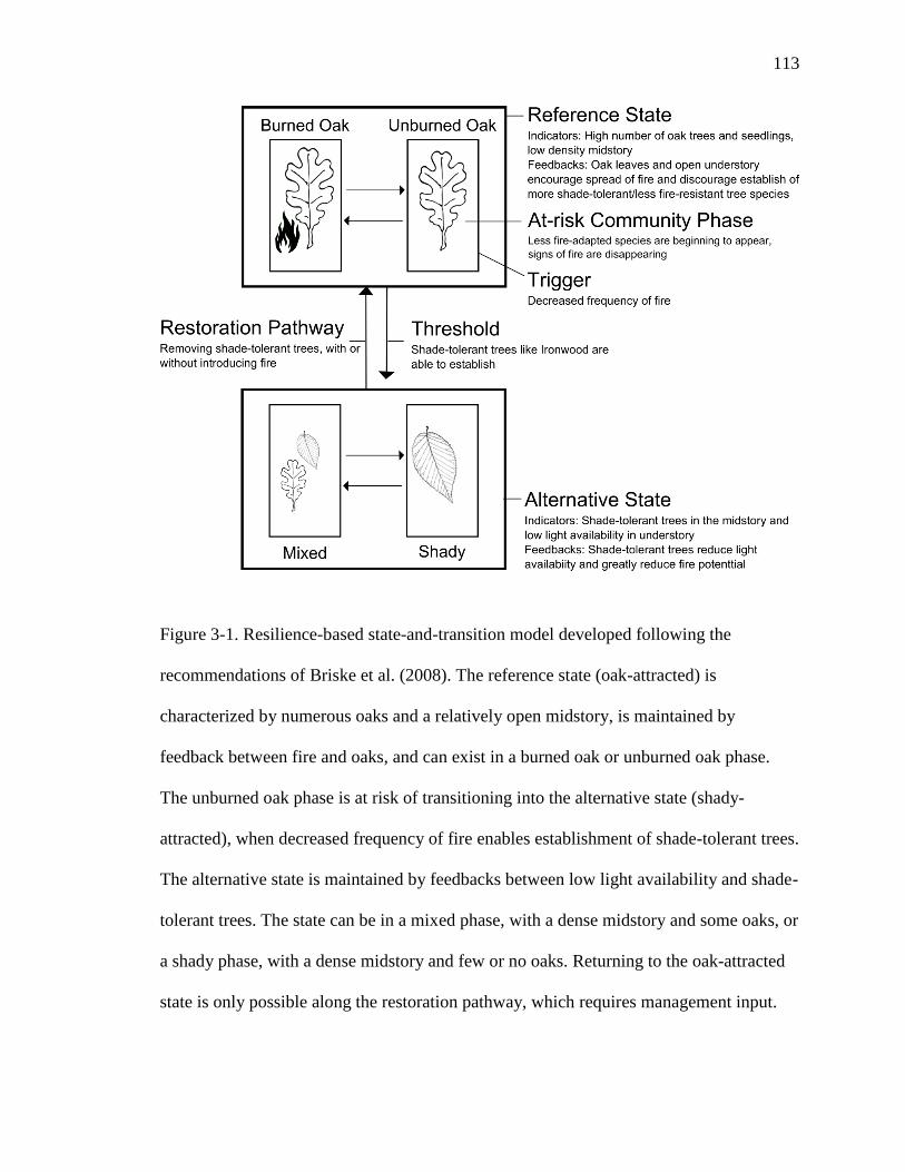
113
Figure 3-1. Resilience-based state-and-transition model developed following the
recommendations of Briske et al. (2008). The reference state (oak-attracted) is
characterized by numerous oaks and a relatively open midstory, is maintained by
feedback between fire and oaks, and can exist in a burned oak or unburned oak phase.
The unburned oak phase is at risk of transitioning into the alternative state (shady-
attracted), when decreased frequency of fire enables establishment of shade-tolerant trees.
The alternative state is maintained by feedbacks between low light availability and shade-
tolerant trees. The state can be in a mixed phase, with a dense midstory and some oaks, or
a shady phase, with a dense midstory and few or no oaks. Returning to the oak-attracted
state is only possible along the restoration pathway, which requires management input.
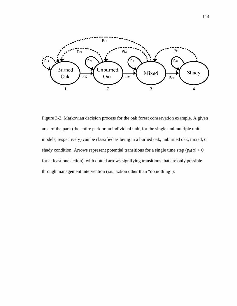
114
Figure 3-2. Markovian decision process for the oak forest conservation example. A given
area of the park (the entire park or an individual unit, for the single and multiple unit
models, respectively) can be classified as being in a burned oak, unburned oak, mixed, or
shady condition. Arrows represent potential transitions for a single time step (pij(a) > 0
for at least one action), with dotted arrows signifying transitions that are only possible
through management intervention (i.e., action other than “do nothing”).
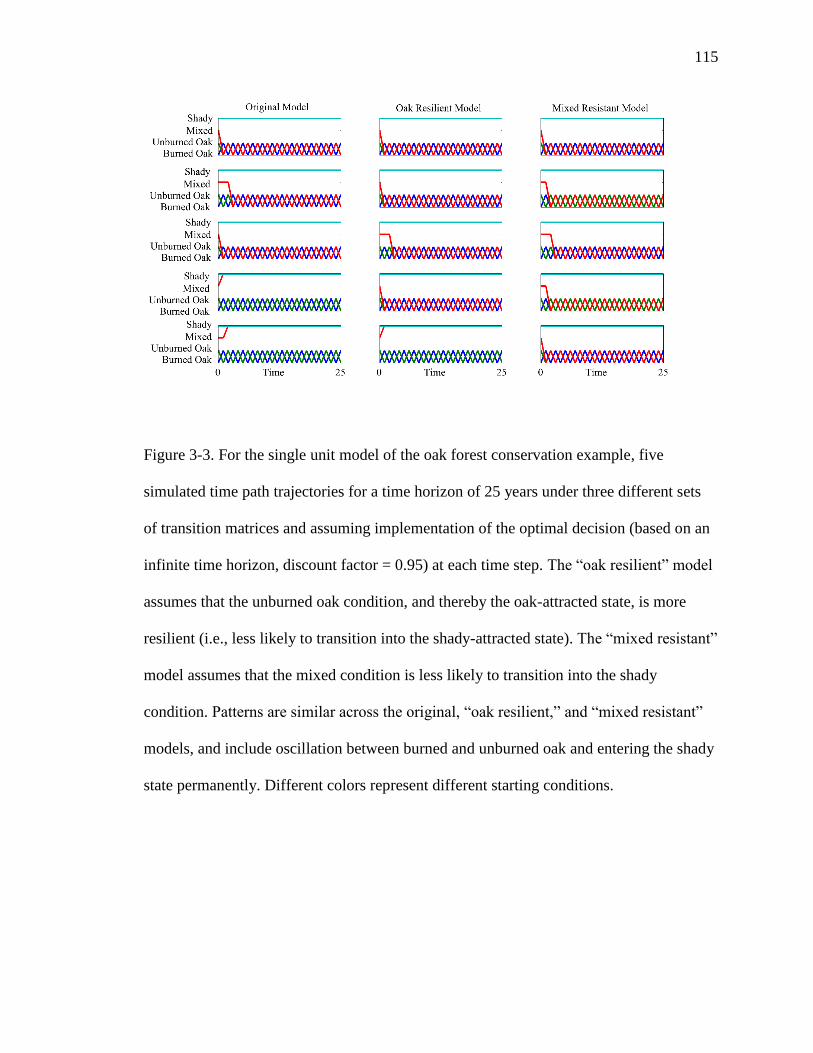
115
Figure 3-3. For the single unit model of the oak forest conservation example, five
simulated time path trajectories for a time horizon of 25 years under three different sets
of transition matrices and assuming implementation of the optimal decision (based on an
infinite time horizon, discount factor = 0.95) at each time step. The “oak resilient” model
assumes that the unburned oak condition, and thereby the oak-attracted state, is more
resilient (i.e., less likely to transition into the shady-attracted state). The “mixed resistant”
model assumes that the mixed condition is less likely to transition into the shady
condition. Patterns are similar across the original, “oak resilient,” and “mixed resistant”
models, and include oscillation between burned and unburned oak and entering the shady
state permanently. Different colors represent different starting conditions.
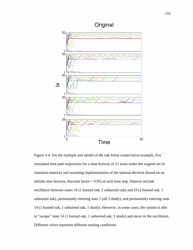
116
Figure 3-4. For the multiple unit model of the oak forest conservation example, five
simulated time path trajectories for a time horizon of 25 years under the original set of
transition matrices and assuming implementation of the optimal decision (based on an
infinite time horizon, discount factor = 0.95) at each time step. Patterns include
oscillation between states 16 (1 burned oak, 2 unburned oak) and 19 (2 burned oak, 1
unburned oak), permanently entering state 1 (all 3 shady), and permanently entering state
14 (1 burned oak, 1 unburned oak, 1 shady). However, in some cases, the system is able
to “escape” state 14 (1 burned oak, 1 unburned oak, 1 shady) and move to the oscillation.
Different colors represent different starting conditions.

117
Figure 3-5. For the multiple unit model of the oak forest conservation example, five
simulated time path trajectories for a time horizon of 25 years under the “oak resilient”
set of transition matrices (for which the unburned oak condition is less likely to transition
to the mixed condition) and assuming implementation of the optimal decision (based on
an infinite time horizon, discount factor = 0.95) at each time step. Patterns include
oscillation between states 16 (1 burned oak, 2 unburned oak) and 19 (2 burned oak, 1
unburned oak), permanently entering state 1 (all 3 shady), and permanently entering state
14 (1 burned oak, 1 unburned oak, 1 shady). However, in some cases, the system is able
to “escape” state 14 (1 burned oak, 1 unburned oak, 1 shady) and move to the oscillation.
Different colors represent different starting conditions.
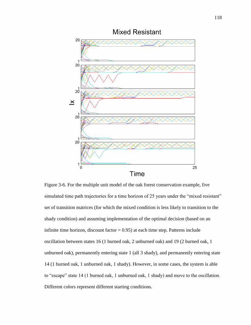
118
Figure 3-6. For the multiple unit model of the oak forest conservation example, five
simulated time path trajectories for a time horizon of 25 years under the “mixed resistant”
set of transition matrices (for which the mixed condition is less likely to transition to the
shady condition) and assuming implementation of the optimal decision (based on an
infinite time horizon, discount factor = 0.95) at each time step. Patterns include
oscillation between states 16 (1 burned oak, 2 unburned oak) and 19 (2 burned oak, 1
unburned oak), permanently entering state 1 (all 3 shady), and permanently entering state
14 (1 burned oak, 1 unburned oak, 1 shady). However, in some cases, the system is able
to “escape” state 14 (1 burned oak, 1 unburned oak, 1 shady) and move to the oscillation.
Different colors represent different starting conditions.
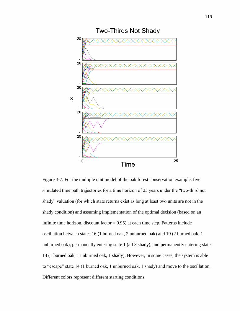
119
Figure 3-7. For the multiple unit model of the oak forest conservation example, five
simulated time path trajectories for a time horizon of 25 years under the “two-third not
shady” valuation (for which state returns exist as long at least two units are not in the
shady condition) and assuming implementation of the optimal decision (based on an
infinite time horizon, discount factor = 0.95) at each time step. Patterns include
oscillation between states 16 (1 burned oak, 2 unburned oak) and 19 (2 burned oak, 1
unburned oak), permanently entering state 1 (all 3 shady), and permanently entering state
14 (1 burned oak, 1 unburned oak, 1 shady). However, in some cases, the system is able
to “escape” state 14 (1 burned oak, 1 unburned oak, 1 shady) and move to the oscillation.
Different colors represent different starting conditions.

120
Figure 3-8. For the multiple unit model of the oak forest conservation example, five
simulated time path trajectories for a time horizon of 25 years under the “no shady”
valuation (for which state returns are equivalent and non-zero when no unit is shady, and
zero otherwise) and assuming implementation of the optimal decision (based on an
infinite time horizon, discount factor = 0.95) at each time step. Similar to the original
valuation results, patterns include an oscillation between states 16 (1 burned oak, 2
unburned oak) and 19 (2 burned oak, 1 unburned oak) and permanently entering state 1
(all 3 shady).Unlike the original valuation, there is no holding at state 14 (1 burned oak, 1
unburned oak, 1 shady), and there is a new oscillation between state 10 (3 unburned oak)
and state 20 (3 burned oak). Different colors represent different starting conditions.
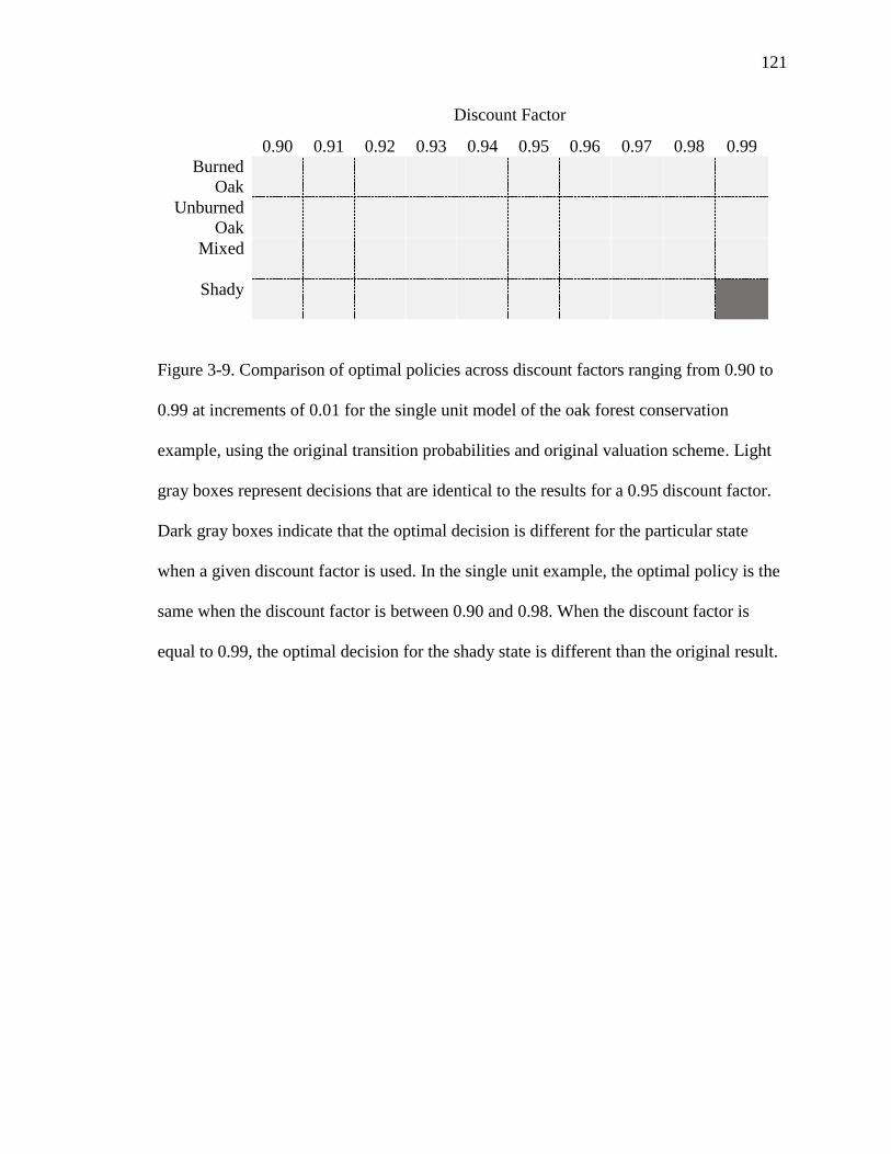
121
Discount Factor
0.90 0.91 0.92 0.93 0.94 0.95 0.96 0.97 0.98 0.99
Burned
Oak
Unburned
Oak
Mixed
Shady
Figure 3-9. Comparison of optimal policies across discount factors ranging from 0.90 to
0.99 at increments of 0.01 for the single unit model of the oak forest conservation
example, using the original transition probabilities and original valuation scheme. Light
gray boxes represent decisions that are identical to the results for a 0.95 discount factor.
Dark gray boxes indicate that the optimal decision is different for the particular state
when a given discount factor is used. In the single unit example, the optimal policy is the
same when the discount factor is between 0.90 and 0.98. When the discount factor is
equal to 0.99, the optimal decision for the shady state is different than the original result.
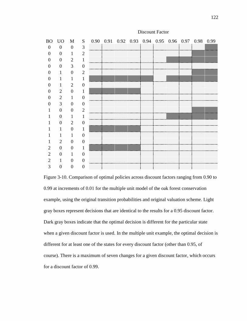
122
Discount Factor
BO UO M S 0.90 0.91 0.92 0.93 0.94 0.95 0.96 0.97 0.98 0.99
0 0 0 3
0 0 1 2
0 0 2 1
0 0 3 0
0 1 0 2
0 1 1 1
0 1 2 0
0 2 0 1
0 2 1 0
0 3 0 0
1 0 0 2
1 0 1 1
1 0 2 0
1 1 0 1
1 1 1 0
1 2 0 0
2 0 0 1
2 0 1 0
2 1 0 0
3 0 0 0
Figure 3-10. Comparison of optimal policies across discount factors ranging from 0.90 to
0.99 at increments of 0.01 for the multiple unit model of the oak forest conservation
example, using the original transition probabilities and original valuation scheme. Light
gray boxes represent decisions that are identical to the results for a 0.95 discount factor.
Dark gray boxes indicate that the optimal decision is different for the particular state
when a given discount factor is used. In the multiple unit example, the optimal decision is
different for at least one of the states for every discount factor (other than 0.95, of
course). There is a maximum of seven changes for a given discount factor, which occurs
for a discount factor of 0.99.
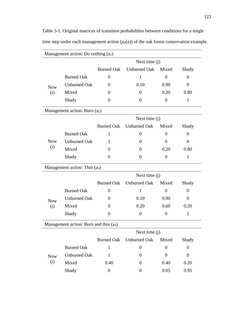
123
Table 3-1. Original matrices of transition probabilities between conditions for a single
time step under each management action (pij(a)) of the oak forest conservation example.
Management action: Do nothing (a1)
Next time (j)
Burned Oak Unburned Oak Mixed Shady
Now
(i)
Burned Oak 0 1 0 0
Unburned Oak 0 0.10 0.90 0
Mixed 0 0 0.20 0.80
Shady
0 0 0 1
Management action: Burn (a2)
Next time (j)
Burned Oak Unburned Oak Mixed Shady
Now
(i)
Burned Oak 1 0 0 0
Unburned Oak 1 0 0 0
Mixed 0 0 0.20 0.80
Shady
0 0 0 1
Management action: Thin (a3)
Next time (j)
Burned Oak Unburned Oak Mixed Shady
Now
(i)
Burned Oak 0 1 0 0
Unburned Oak 0 0.10 0.90 0
Mixed 0 0.20 0.60 0.20
Shady
0 0 0 1
Management action: Burn and thin (a4)
Next time (j)
Burned Oak Unburned Oak Mixed Shady
Now
(i)
Burned Oak 1 0 0 0
Unburned Oak 1 0 0 0
Mixed 0.40 0 0.40 0.20
Shady 0 0 0.05 0.95
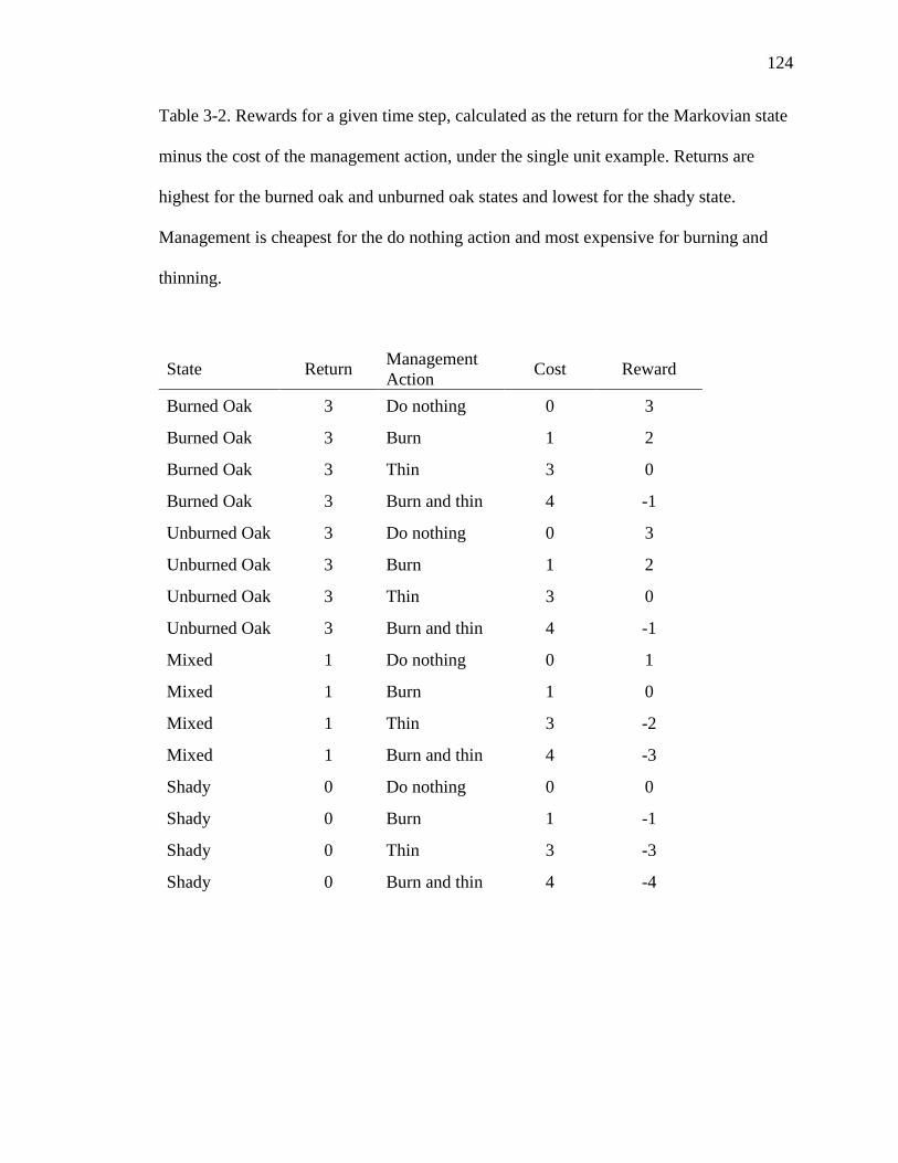
124
Table 3-2. Rewards for a given time step, calculated as the return for the Markovian state
minus the cost of the management action, under the single unit example. Returns are
highest for the burned oak and unburned oak states and lowest for the shady state.
Management is cheapest for the do nothing action and most expensive for burning and
thinning.
State Return Management
Action Cost Reward
Burned Oak 3 Do nothing 0 3
Burned Oak 3 Burn 1 2
Burned Oak 3 Thin 3 0
Burned Oak 3 Burn and thin 4 -1
Unburned Oak 3 Do nothing 0 3
Unburned Oak 3 Burn 1 2
Unburned Oak 3 Thin 3 0
Unburned Oak 3 Burn and thin 4 -1
Mixed 1 Do nothing 0 1
Mixed 1 Burn 1 0
Mixed 1 Thin 3 -2
Mixed 1 Burn and thin 4 -3
Shady 0 Do nothing 0 0
Shady 0 Burn 1 -1
Shady 0 Thin 3 -3
Shady 0 Burn and thin 4 -4

125
Table 3-3. For the single unit model of the oak forest conservation example, optimal
decision and expected value (infinite time horizon, discount = 0.95) for each state when
using the original set of transition probabilities matrices. The greatest expected value
occurs when the park exists in the burned oak state, with similar expected values for the
unburned oak state. Moderate expected values are anticipated when the park exists in the
mixed state. No value is expected when the park exists in the shady state.
State Optimal decision Expected value
Burned Oak Do nothing 50.26
Unburned Oak Burn 49.74
Mixed Burn and thin 25.96
Shady Do nothing 0
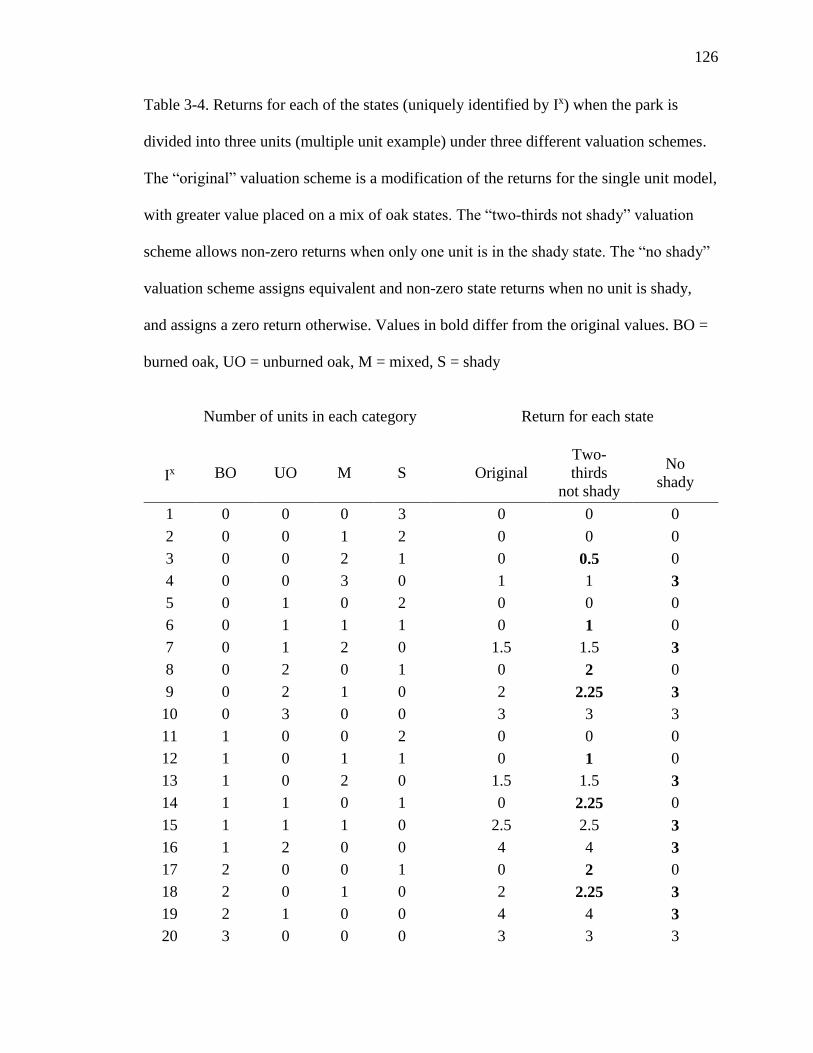
126
Table 3-4. Returns for each of the states (uniquely identified by Ix) when the park is
divided into three units (multiple unit example) under three different valuation schemes.
The “original” valuation scheme is a modification of the returns for the single unit model,
with greater value placed on a mix of oak states. The “two-thirds not shady” valuation
scheme allows non-zero returns when only one unit is in the shady state. The “no shady”
valuation scheme assigns equivalent and non-zero state returns when no unit is shady,
and assigns a zero return otherwise. Values in bold differ from the original values. BO =
burned oak, UO = unburned oak, M = mixed, S = shady
Ix
Number of units in each category Return for each state
BO UO M S Original
Two-
thirds
not shady
No
shady
1 0 0 0 3 0 0 0
2 0 0 1 2 0 0 0
3 0 0 2 1 0 0.5 0
4 0 0 3 0 1 1 3
5 0 1 0 2 0 0 0
6 0 1 1 1 0 1 0
7 0 1 2 0 1.5 1.5 3
8 0 2 0 1 0 2 0
9 0 2 1 0 2 2.25 3
10 0 3 0 0 3 3 3
11 1 0 0 2 0 0 0
12 1 0 1 1 0 1 0
13 1 0 2 0 1.5 1.5 3
14 1 1 0 1 0 2.25 0
15 1 1 1 0 2.5 2.5 3
16 1 2 0 0 4 4 3
17 2 0 0 1 0 2 0
18 2 0 1 0 2 2.25 3
19 2 1 0 0 4 4 3
20 3 0 0 0 3 3 3
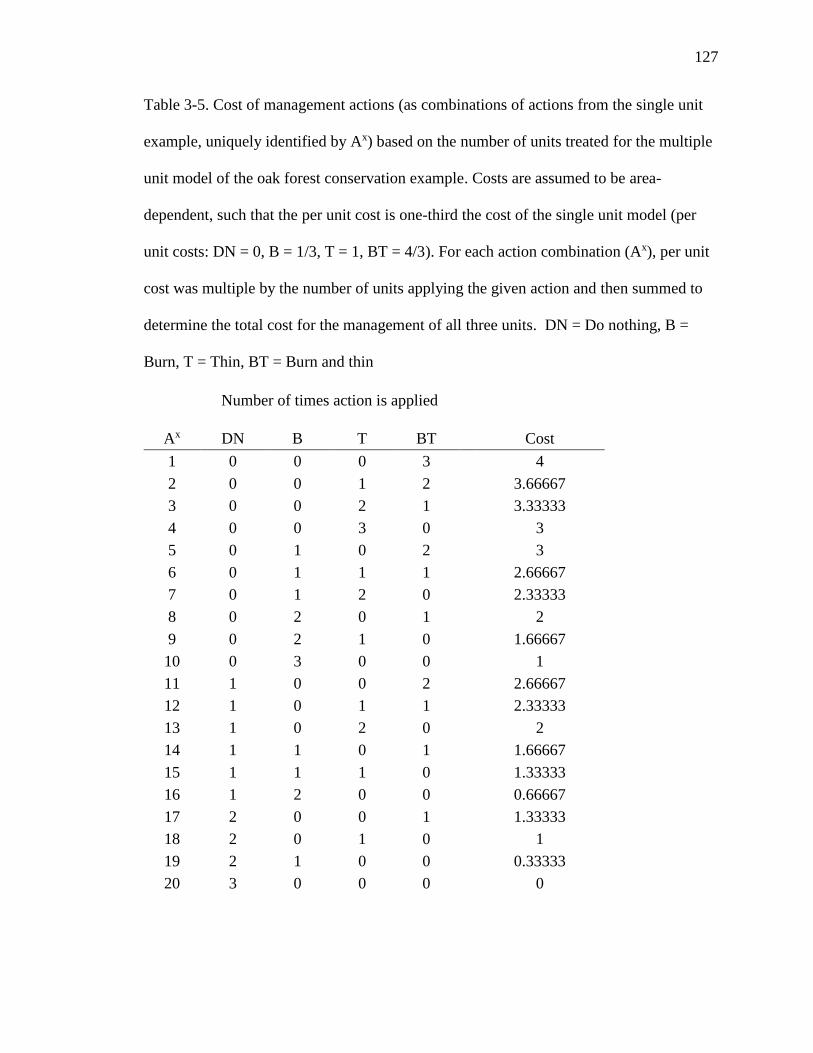
127
Table 3-5. Cost of management actions (as combinations of actions from the single unit
example, uniquely identified by Ax) based on the number of units treated for the multiple
unit model of the oak forest conservation example. Costs are assumed to be area-
dependent, such that the per unit cost is one-third the cost of the single unit model (per
unit costs: DN = 0, B = 1/3, T = 1, BT = 4/3). For each action combination (Ax), per unit
cost was multiple by the number of units applying the given action and then summed to
determine the total cost for the management of all three units. DN = Do nothing, B =
Burn, T = Thin, BT = Burn and thin
Ax
Number of times action is applied
DN B T BT Cost
1 0 0 0 3 4
2 0 0 1 2 3.66667
3 0 0 2 1 3.33333
4 0 0 3 0 3
5 0 1 0 2 3
6 0 1 1 1 2.66667
7 0 1 2 0 2.33333
8 0 2 0 1 2
9 0 2 1 0 1.66667
10 0 3 0 0 1
11 1 0 0 2 2.66667
12 1 0 1 1 2.33333
13 1 0 2 0 2
14 1 1 0 1 1.66667
15 1 1 1 0 1.33333
16 1 2 0 0 0.66667
17 2 0 0 1 1.33333
18 2 0 1 0 1
19 2 1 0 0 0.33333
20 3 0 0 0 0
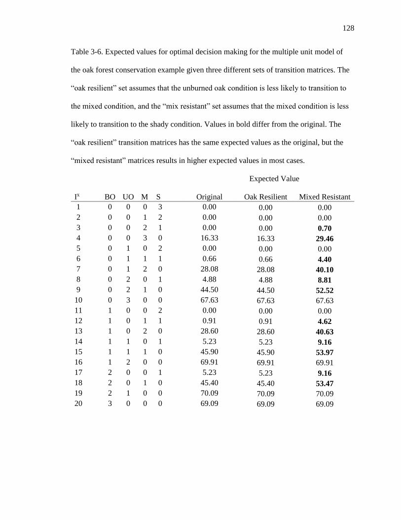
128
Table 3-6. Expected values for optimal decision making for the multiple unit model of
the oak forest conservation example given three different sets of transition matrices. The
“oak resilient” set assumes that the unburned oak condition is less likely to transition to
the mixed condition, and the “mix resistant” set assumes that the mixed condition is less
likely to transition to the shady condition. Values in bold differ from the original. The
“oak resilient” transition matrices has the same expected values as the original, but the
“mixed resistant” matrices results in higher expected values in most cases.
Expected Value
Ix BO UO M S Original Oak Resilient Mixed Resistant
1 0 0 0 3 0.00 0.00 0.00
2 0 0 1 2 0.00 0.00 0.00
3 0 0 2 1 0.00 0.00 0.70
4 0 0 3 0 16.33 16.33 29.46
5 0 1 0 2 0.00 0.00 0.00
6 0 1 1 1 0.66 0.66 4.40
7 0 1 2 0 28.08 28.08 40.10
8 0 2 0 1 4.88 4.88 8.81
9 0 2 1 0 44.50 44.50 52.52
10 0 3 0 0 67.63 67.63 67.63
11 1 0 0 2 0.00 0.00 0.00
12 1 0 1 1 0.91 0.91 4.62
13 1 0 2 0 28.60 28.60 40.63
14 1 1 0 1 5.23 5.23 9.16
15 1 1 1 0 45.90 45.90 53.97
16 1 2 0 0 69.91 69.91 69.91
17 2 0 0 1 5.23 5.23 9.16
18 2 0 1 0 45.40 45.40 53.47
19 2 1 0 0 70.09 70.09 70.09
20 3 0 0 0 69.09 69.09 69.09
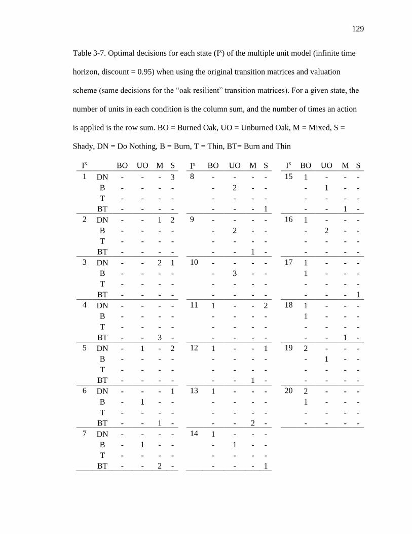
129
Table 3-7. Optimal decisions for each state (Ix) of the multiple unit model (infinite time
horizon, discount = 0.95) when using the original transition matrices and valuation
scheme (same decisions for the “oak resilient” transition matrices). For a given state, the
number of units in each condition is the column sum, and the number of times an action
is applied is the row sum. BO = Burned Oak, UO = Unburned Oak, M = Mixed, S =
Shady, DN = Do Nothing, B = Burn, T = Thin, BT= Burn and Thin
Ix BO UO M S Ix BO UO M S Ix BO UO M S
1 DN - - - 3 8 - - - - 15 1 - - -
B - - - - - 2 - - - 1 - -
T - - - - - - - - - - - -
BT - - - - - - - 1 - - 1 -
2 DN - - 1 2 9 - - - - 16 1 - - -
B - - - - - 2 - - - 2 - -
T - - - - - - - - - - - -
BT - - - - - - 1 - - - - -
3 DN - - 2 1 10 - - - - 17 1 - - -
B - - - - - 3 - - 1 - - -
T - - - - - - - - - - - -
BT - - - - - - - - - - - 1
4 DN - - - - 11 1 - - 2 18 1 - - -
B - - - - - - - - 1 - - -
T - - - - - - - - - - - -
BT - - 3 - - - - - - - 1 -
5 DN - 1 - 2 12 1 - - 1 19 2 - - -
B - - - - - - - - - 1 - -
T - - - - - - - - - - - -
BT - - - - - - 1 - - - - -
6 DN - - - 1 13 1 - - - 20 2 - - -
B - 1 - - - - - - 1 - - -
T - - - - - - - - - - - -
BT - - 1 - - - 2 - - - - -
7 DN - - - - 14 1 - - -
B - 1 - - - 1 - -
T - - - - - - - -
BT - - 2 - - - - 1
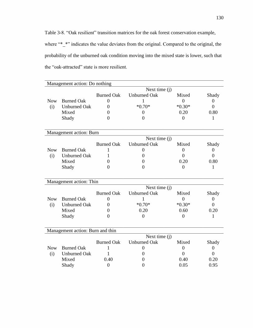
130
Table 3-8. “Oak resilient” transition matrices for the oak forest conservation example,
where “*_*” indicates the value deviates from the original. Compared to the original, the
probability of the unburned oak condition moving into the mixed state is lower, such that
the “oak-attracted” state is more resilient.
Management action: Do nothing
Next time (j)
Burned Oak Unburned Oak Mixed Shady
Now
(i)
Burned Oak 0 1 0 0
Unburned Oak 0 *0.70* *0.30* 0
Mixed 0 0 0.20 0.80
Shady 0 0 0 1
Management action: Burn
Next time (j)
Burned Oak Unburned Oak Mixed Shady
Now
(i)
Burned Oak 1 0 0 0
Unburned Oak 1 0 0 0
Mixed 0 0 0.20 0.80
Shady 0 0 0 1
Management action: Thin
Next time (j)
Burned Oak Unburned Oak Mixed Shady
Now
(i)
Burned Oak 0 1 0 0
Unburned Oak 0 *0.70* *0.30* 0
Mixed 0 0.20 0.60 0.20
Shady 0 0 0 1
Management action: Burn and thin
Next time (j)
Burned Oak Unburned Oak Mixed Shady
Now
(i)
Burned Oak 1 0 0 0
Unburned Oak 1 0 0 0
Mixed 0.40 0 0.40 0.20
Shady 0 0 0.05 0.95

131
Table 3-9. “Mixed resistant” transition matrices for the oak forest conservation example,
where “*_*” indicates the value deviates from the original. Compared to the original, the
probability of the mixed condition transitioning into the shady state is lower.
Management action: Do nothing
Next time (j)
Burned Oak Unburned Oak Mixed Shady
Now
(i)
Burned Oak 0 1 0 0
Unburned Oak 0 0.10 0.90 0
Mixed 0 0 *0.70* *0.30*
Shady 0 0 0 1
Management action: Burn
Next time (j)
Burned Oak Unburned Oak Mixed Shady
Now
(i)
Burned Oak 1 0 0 0
Unburned Oak 1 0 0 0
Mixed 0 0 *0.70* *0.30*
Shady 0 0 0 1
Management action: Thin
Next time (j)
Burned Oak Unburned Oak Mixed Shady
Now
(i)
Burned Oak 0 1 0 0
Unburned Oak 0 0.10 0.90 0
Mixed 0 0.20 *0.70* *0.10*
Shady 0 0 0 1
Management action: Burn and thin
Next time (j)
Burned Oak Unburned Oak Mixed Shady
Now
(i)
Burned Oak 1 0 0 0
Unburned Oak 1 0 0 0
Mixed 0.40 0 *0.50* *0.10*
Shady 0 0 0.05 0.95

132
Table 3-10. Optimal decision and expected values for the single unit example of the oak
forest conservation example under the different transition matrices (original || oak
resilient || mixed resistant). The “oak resilient” set assumes that the unburned oak
condition is less likely to transition to the mixed condition, and the “mix resistant” set
assumes that the mixed condition is less likely to transition to the shady condition. All
optimal decisions are the same, and the only expected value that is different is for the
mixed condition under the mixed resistant matrices (in bold).
Optimal Decision
State Original
Oak
Resilient
Mixed
Resistant Expected value
Burned Oak Do nothing Do nothing Do nothing 50.26 || 50.26 || 50.26
Unburned Oak Burn Burn Burn 49.74 || 49.74 || 49.74
Mixed Burn and
thin
Burn and
thin
Burn and
thin 25.96 || 25.96 || 30.66
Shady Do nothing Do nothing Do nothing 0 || 0 || 0

133
Table 3-11. Optimal decisions for each state (Ix) (infinite time horizon, discount = 0.95)
for the multiple unit model using the “mixed resistant” transition matrices and original
valuation scheme. Underlined states indicate decisions different from the original. For a
given state, the number of units in each condition is the column sum, and the number of
times an action is applied is the row sum. BO = Burned Oak, UO = Unburned Oak, M =
Mixed, S = Shady, DN = Do Nothing, B = Burn, T = Thin, BT= Burn and Thin
Ix BO UO M S Ix BO UO M S Ix BO UO M S
1 DN - - - 3 8 - - - - 15 1 - - -
B - - - - - 2 - - - 1 - -
T - - - - - - - - - - - -
BT - - - - - - - 1 - - 1 -
2 DN - - 1 2 9 - - - - 16 1 - - -
B - - - - - 2 - - - 2 - -
T - - - - - - - - - - - -
BT - - - - - - 1 - - - - -
3 DN - - - - 10 - - - - 17 1 - - -
B - - - - - 3 - - 1 - - -
T - - - - - - - - - - - -
BT - - 2 1 - - - - - - - 1
4 DN - - - - 11 1 - - 2 18 1 - - -
B - - - - - - - - 1 - - -
T - - - - - - - - - - - -
BT - - 3 - - - - - - - 1 -
5 DN - 1 - 2 12 1 - - - 19 2 - - -
B - - - - - - - - - 1 - -
T - - - - - - - - - - - -
BT - - - - - - 1 1 - - - -
6 DN - - - - 13 1 - - - 20 2 - - -
B - 1 - - - - - - 1 - - -
T - - - - - - - - - - - -
BT - - 1 1 - - 2 - - - - -
7 DN - - - - 14 1 - - -
B - 1 - - - 1 - -
T - - - - - - - -
BT - - 2 - - - - 1
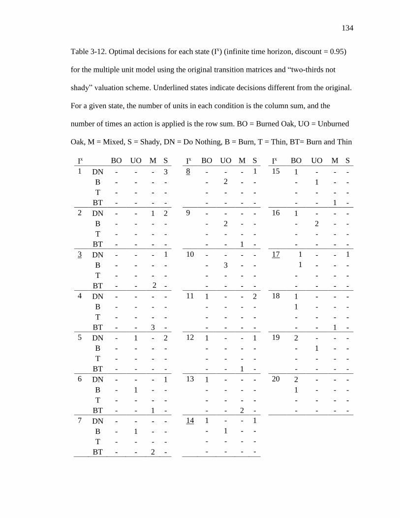
134
Table 3-12. Optimal decisions for each state (Ix) (infinite time horizon, discount = 0.95)
for the multiple unit model using the original transition matrices and “two-thirds not
shady” valuation scheme. Underlined states indicate decisions different from the original.
For a given state, the number of units in each condition is the column sum, and the
number of times an action is applied is the row sum. BO = Burned Oak, UO = Unburned
Oak, M = Mixed, S = Shady, DN = Do Nothing, B = Burn, T = Thin, BT= Burn and Thin
Ix BO UO M S Ix BO UO M S Ix BO UO M S
1 DN - - - 3 8 - - - 1 15 1 - - -
B - - - - - 2 - - - 1 - -
T - - - - - - - - - - - -
BT - - - - - - - - - - 1 -
2 DN - - 1 2 9 - - - - 16 1 - - -
B - - - - - 2 - - - 2 - -
T - - - - - - - - - - - -
BT - - - - - - 1 - - - - -
3 DN - - - 1 10 - - - - 17 1 - - 1
B - - - - - 3 - - 1 - - -
T - - - - - - - - - - - -
BT - - 2 - - - - - - - - -
4 DN - - - - 11 1 - - 2 18 1 - - -
B - - - - - - - - 1 - - -
T - - - - - - - - - - - -
BT - - 3 - - - - - - - 1 -
5 DN - 1 - 2 12 1 - - 1 19 2 - - -
B - - - - - - - - - 1 - -
T - - - - - - - - - - - -
BT - - - - - - 1 - - - - -
6 DN - - - 1 13 1 - - - 20 2 - - -
B - 1 - - - - - - 1 - - -
T - - - - - - - - - - - -
BT - - 1 - - - 2 - - - - -
7 DN - - - - 14 1 - - 1
B - 1 - - - 1 - -
T - - - - - - - -
BT - - 2 - - - - -
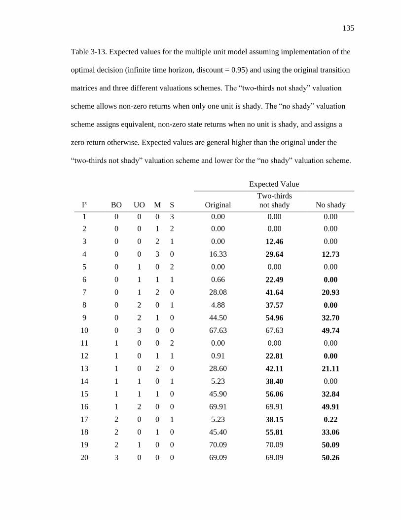
135
Table 3-13. Expected values for the multiple unit model assuming implementation of the
optimal decision (infinite time horizon, discount = 0.95) and using the original transition
matrices and three different valuations schemes. The “two-thirds not shady” valuation
scheme allows non-zero returns when only one unit is shady. The “no shady” valuation
scheme assigns equivalent, non-zero state returns when no unit is shady, and assigns a
zero return otherwise. Expected values are general higher than the original under the
“two-thirds not shady” valuation scheme and lower for the “no shady” valuation scheme.
Expected Value
Ix BO UO M S Original
Two-thirds
not shady No shady
1 0 0 0 3 0.00 0.00 0.00
2 0 0 1 2 0.00 0.00 0.00
3 0 0 2 1 0.00 12.46 0.00
4 0 0 3 0 16.33 29.64 12.73
5 0 1 0 2 0.00 0.00 0.00
6 0 1 1 1 0.66 22.49 0.00
7 0 1 2 0 28.08 41.64 20.93
8 0 2 0 1 4.88 37.57 0.00
9 0 2 1 0 44.50 54.96 32.70
10 0 3 0 0 67.63 67.63 49.74
11 1 0 0 2 0.00 0.00 0.00
12 1 0 1 1 0.91 22.81 0.00
13 1 0 2 0 28.60 42.11 21.11
14 1 1 0 1 5.23 38.40 0.00
15 1 1 1 0 45.90 56.06 32.84
16 1 2 0 0 69.91 69.91 49.91
17 2 0 0 1 5.23 38.15 0.22
18 2 0 1 0 45.40 55.81 33.06
19 2 1 0 0 70.09 70.09 50.09
20 3 0 0 0 69.09 69.09 50.26

136
Table 3-14. Optimal decisions for each state (Ix) (infinite time horizon, discount = 0.95)
for the multiple unit model using the original transition matrices and “no shady”
valuation scheme. Underlined states indicate decisions different from the original. For a
given state, the number of units in each condition is the column sum, and the number of
times an action is applied is the row sum. BO = Burned Oak, UO = Unburned Oak, M =
Mixed, S = Shady, DN = Do Nothing, B = Burn, T = Thin, BT= Burn and Thin
Ix BO UO M S Ix BO UO M S Ix BO UO M S
1 DN - - - 3 8 - 2 - 1 15 1 - - -
B - - - - - - - - - 1 - -
T - - - - - - - - - - - -
BT - - - - - - - - - - 1 -
2 DN - - 1 2 9 - - - - 16 1 - - -
B - - - - - 2 - - - 2 - -
T - - - - - - - - - - - -
BT - - - - - - 1 - - - - -
3 DN - - 2 1 10 - - - - 17 2 - - -
B - - - - - 3 - - - - - -
T - - - - - - - - - - - -
BT - - - - - - - - - - - 1
4 DN - - - - 11 1 - - 2 18 2 - - -
B - - - - - - - - - - - -
T - - - - - - - - - - - -
BT - - 3 - - - - - - - 1 -
5 DN - 1 - 2 12 1 - 1 1 19 2 - - -
B - - - - - - - - - 1 - -
T - - - - - - - - - - - -
BT - - - - - - - - - - - -
6 DN - 1 1 1 13 1 - - - 20 3 - - -
B - - - - - - - - - - - -
T - - - - - - - - - - - -
BT - - - - - - 2 - - - - -
7 DN - - - - 14 1 1 - 1
B - 1 - - - - - -
T - - - - - - - -
BT - - 2 - - - - -
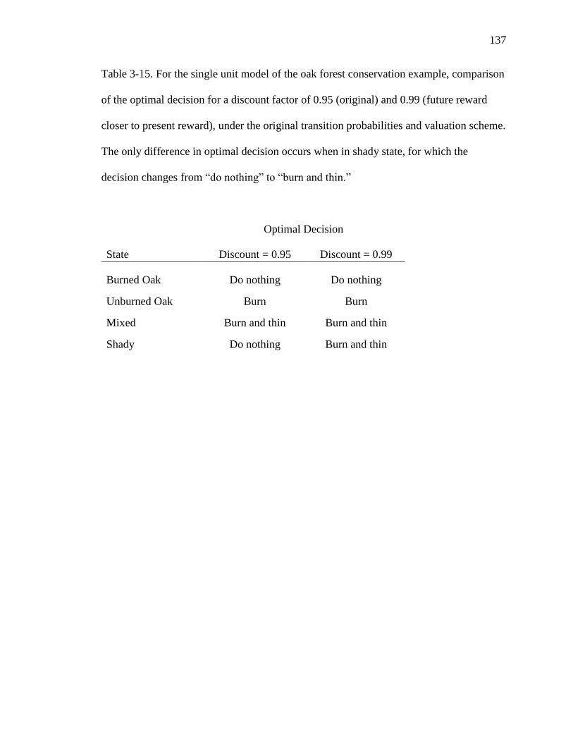
137
Table 3-15. For the single unit model of the oak forest conservation example, comparison
of the optimal decision for a discount factor of 0.95 (original) and 0.99 (future reward
closer to present reward), under the original transition probabilities and valuation scheme.
The only difference in optimal decision occurs when in shady state, for which the
decision changes from “do nothing” to “burn and thin.”
Optimal Decision
State Discount = 0.95 Discount = 0.99
Burned Oak Do nothing Do nothing
Unburned Oak Burn Burn
Mixed Burn and thin Burn and thin
Shady Do nothing Burn and thin

138
Table 3-16. For the multiple unit model of the oak forest conservation example,
comparison of the optimal decision for a discount factor of 0.95 (original) and 0.90
(future reward further discounted), under the original transition probabilities and
valuation scheme. States (Ix) that are not listed have the same decision as the original
multiple unit example. BO = Burned Oak, UO = Unburned Oak, M = Mixed, S = Shady,
DN = Do Nothing, B = Burn, T = Thin, BT= Burn and Thin
Discount = 0.95 Discount = 0.90
Ix BO UO M S BO UO M S
6 DN - - - 1 - 1 1 1
B - 1 - - - - - -
T - - - - - - - -
BT - - 1 - - - - -
8 DN - - - - - 2 - 1
B - 2 - - - - - -
T - - - - - - - -
BT - - - 1 - - - -
14 DN 1 - - - 1 1 - 1
B - 1 - - - - - -
T - - - - - - - -
BT - - - 1 - - - -
17 DN 1 - - - 2 - - 1
B 1 - - - - - - -
T - - - - - - - -
BT - - - 1 - - - -

139
Table 3-17. For the multiple unit model of the oak forest conservation example,
comparison of the optimal decision for a discount factor of 0.95 (original) and 0.99
(future reward closer to present reward), under the original transition probabilities and
valuation scheme. States (Ix) that are not listed have the same decision as the original
multiple unit example. BO = Burned Oak, UO = Unburned Oak, M = Mixed, S = Shady,
DN = Do Nothing, B = Burn, T = Thin, BT= Burn and Thin
Discount = 0.95 Discount = 0.99
Ix BO UO M S BO UO M S
1 DN - - - 3 - - - -
B - - - - - - - -
T - - - - - - - -
BT - - - - - - - 3
2 DN - - 1 2 - - - -
B - - - - - - - -
T - - - - - - - -
BT - - - - - - 1 2
3 DN - - 2 1 - - - -
B - - - - - - - -
T - - - - - - - -
BT - - - - - - 2 1
5 DN - 1 - 2 - - - -
B - - - - - 1 - -
T - - - - - - - -
BT - - - - - - - 2
6 DN - - - 1 - - - -
B - 1 - - - 1 - -
T - - - - - - - -
BT - - 1 - - - 1 1
11 DN 1 - - 2 1 - - -
B - - - - - - - -
T - - - - - - - -
BT - - - - - - - 2
12 DN 1 - - 1 1 - - -
B - - - - - - - -
T - - - - - - - -
BT - - 1 - - - 1 1
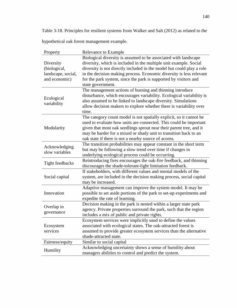
140
Table 3-18. Principles for resilient systems from Walker and Salt (2012) as related to the
hypothetical oak forest management example.
Property Relevance to Example
Diversity
(biological,
landscape, social,
and economic)
Biological diversity is assumed to be associated with landscape
diversity, which is included in the multiple unit example. Social
diversity is not directly included in the model but could play a role
in the decision making process. Economic diversity is less relevant
for the park system, since the park is supported by visitors and
state government.
Ecological
variability
The management actions of burning and thinning introduce
disturbance, which encourages variability. Ecological variability is
also assumed to be linked to landscape diversity. Simulations
allow decision makers to explore whether there is variability over
time.
Modularity
The category count model is not spatially explicit, so it cannot be
used to evaluate how units are connected. This could be important
given that most oak seedlings sprout near their parent tree, and it
may be harder for a mixed or shady unit to transition back to an
oak state if there is not a nearby source of acorns.
Acknowledging
slow variables
The transition probabilities may appear constant in the short term
but may be following a slow trend over time if changes in
underlying ecological process could be occurring.
Tight feedbacks Reintroducing fires encourages the oak-fire feedback, and thinning
discourages the shade-tolerant-light limitation feedback.
Social capital
If stakeholders, with different values and mental models of the
system, are included in the decision making process, social capital
may be increased.
Innovation
Adaptive management can improve the system model. It may be
possible to set aside portions of the park to set-up experiments and
expedite the rate of learning.
Overlap in
governance
Decision making in the park is nested within a larger state park
agency. Private properties surround the park, such that the region
includes a mix of public and private rights.
Ecosystem
services
Ecosystem services were implicitly used to define the values
associated with ecological states. The oak-attracted forest is
assumed to provide greater ecosystem services than the alternative
shade-attracted state.
Fairness/equity Similar to social capital
Humility Acknowledging uncertainty shows a sense of humility about
managers abilities to control and predict the system.
141
CHAPTER 4: INCORPORATING ADAPTIVE MANAGEMENT INTO STATE
WILDLIFE ACTION PLANS
1. INTRODUCTION
State Wildlife Action Plans present status assessments and conservation strategies
for wildlife, including non-game species, and their habitats in an effort to avoid the listing
of species under the Endangered Species Act (Department of Interior and Related
Agencies Appropriations Act 2002, AFWA 2014); this is colloquially known as “keeping
common species common.” Congress stipulated that State Wildlife Grant funding be
contingent upon development of State Wildlife Action Plans (i.e., “comprehensive
wildlife conservation plans”) that contain eight mandatory elements (Table 4-1) (Wildlife
Conservation and Restoration and State Wildlife Programs 2001, Department of Interior
and Related Agencies Appropriations Act 2002, AFWA 2014). While not explicitly
requiring structured decision making or adaptive management, the eight State Wildlife
Action Plan elements easily fit these approaches (Fontaine 2011).
Structured decision making is a process for making transparent, defensible
decisions that define the particular problem and identify clear objectives, alternatives,
consequences, and tradeoffs (Hammond et al. 1999, Gregory et al. 2012). Most
management projects can benefit from the focus and organization structured decision
making provides relative to ad hoc, technical solution-oriented decision making (Conroy
and Peterson 2013). Adaptive management is a special form of structured decision
making (e.g., Walters 1986, Lyons et al. 2008, Martin et al. 2009, Williams et al. 2009,
Conroy and Peterson 2013) in which uncertainty about management effects is
142
deliberately reduced through monitoring and analysis to improve effectiveness of future
efforts (Holling 1978, Walters 1986, Lyons et al. 2008, Williams et al. 2009). The
required State Wildlife Action Plan elements of identifying problems and actions and
planning monitoring/adjustment match the components of structured decision making and
adaptive management, yet no State Wildlife Action Plan currently includes an explicit
structured decision making or adaptive management framework for immediate project
design and implementation for specific taxa, habitats, or threats (Fontaine 2011). There
are many possible reasons explicit frameworks may be missing. For example, managers
may believe they are already doing adaptive management, there may be an underlying
assumption that adaptive management is impractical, or there may be limited experience
in planning and implementing structured decision making and adaptive management.
Adaptive management may be critical for conserving wildlife and their habitats,
as managers increasingly recognize the prevalence of uncertainty and the potential for
unforeseen consequences (e.g., Murphy and Noon 1991, Williams 2001, Regan et al.
2005, Runge et al. 2011). Although learning while managing seems like common sense
(Holling 1978), adaptive management is not appropriate or possible in all situations, and
there is a rich literature on barriers to successful adaptive management (e.g., Gunderson
et al. 1995, Walters 1997, Gregory et al. 2006, Allen and Gunderson 2011).
Misapplication of adaptive management can jeopardize natural resources (Doremus
2001), and if failure is falsely attributed to the adaptive management process itself, this
may dissuade future uses of adaptive management (Loftin 2014), even in suitable
circumstances.

143
In order to successfully use adaptive management to achieve State Wildlife
Action Plan conservation goals, planners must be able to apply structured decision
making, identify appropriate situations for adaptive management, and design specific
projects that facilitate learning and adjusting. This chapter presents: (a) a brief overview
of structured decision making, including adaptive management, (b) a dichotomous key
for efficient, critical thinking about when adaptive management may be appropriate, and
(c) a preliminary guide for designing an adaptive management project. I then use
Nebraska’s State Wildlife Action Plan, also known as the Nebraska Natural Legacy
Project (Schneider et al. 2011), as a case study to illustrate how current planning
strategies can be adapted to structured decision making and to discuss the potential for
adaptive management projects based on recent planning efforts. Although other guides
exist for structured decision making (e.g., Gregory et al. 2012, Conroy and Peterson
2013) and adaptive management (e.g., Gregory et al. 2006, Williams et al. 2009), my
approach is specifically tailored to providing guidance for developing adaptive
management projects in the context of State Wildlife Action Plans and includes relevant
examples.
2. BRIEF OVERVIEW OF STRUCTURED DECISION MAKING AND
ADAPTIVE MANAGEMENT
Structured decision making is a process for making transparent, defensible
decisions (Hammond et al. 1999, Gregory and Keeney 2002, Gregory et al. 2012), which
differs from ad hoc, technical solution-oriented decision making that often guides natural
resource management (Conroy and Peterson 2013). The steps involve: 1) defining the
144
problem, 2) determining objectives, 3) outlining alternatives, 4) considering the
consequences, and 5) understanding the tradeoffs (Figure 4-1). The problem definition
clarifies the decision context and lays out the scope of the project. Objectives express the
components of success and the desired direction of change (Gregory et al. 2012).
Objectives can be divided into fundamental and means objectives, where fundamental
objectives are what is truly valued and means objectives are important only insofar as
they help achieve fundamental objectives (Conroy and Peterson 2013). Alternatives are
the management options under consideration. Consequences describe how an alternative
is predicted to contribute to the objectives (Gregory et al. 2012). Unless one alternative
achieves every objective better than the other alternatives, tradeoffs will have to be made
(Gregory et al. 2012). Under some descriptions of structured decision making, the
consequences step is part of a “develop models” step, with tradeoffs treated by assigning
weights to objectives (e.g., Williams et al. 2009, Conroy and Peterson 2013). Modeling is
a key tool of structured decision making, where models are loosely defined by Conroy
and Peterson (2013) as “any conceptualization of the relationship between decisions,
outcomes, and other factors.”
Adaptive management can be viewed as a special form of structured decision
making in which iterative decisions are made based on knowledge gained from results of
previous decisions. The process builds on the original five steps by: 6) monitoring
outcomes, 7) analyzing the data, and 8) adjusting management based on learning (Lyons
et al. 2008, Williams et al. 2009, Allen et al. 2011). Adaptive management allows
management to proceed despite uncertain consequences and treats management as a
continual learning process (Walters 1986). The most basic requirements of adaptive
145
management are a) deliberate learning through management, and b) changing
management to reflect what is learned (Walters and Holling 1990, Williams and Brown
2012). Learning, in this case, means the reduction of uncertainty. Although many types of
uncertainties exist, adaptive management is concerned with uncertainties related to how
systems or species respond to management and the particular mechanisms driving
observed responses (Williams et al. 2009).
3. WHEN TO USE ADAPTIVE MANAGEMENT FOR A STATE WILDLIFE
ACTION PLAN
Adaptive management is not always possible or appropriate. There are many
barriers to successful adaptive management (Gunderson et al. 1995, Walters 1997,
Gregory et al. 2006, Williams et al. 2009, Allen and Gunderson 2011), among them
irresolvable conflict, uncontrollability, and inability to sufficiently monitor (Williams et
al. 2009). Given the plethora of wildlife management uncertainties and limitations of
adaptive management, wildlife managers designing State Wildlife Action Plan projects
may benefit from a quick way to determine when adaptive management should be
considered. I developed a brief dichotomous key as an organized, question-based
approach to narrowing down a generated list of uncertainties to those best suited for
adaptive management projects within a State Wildlife Action Plan (Figure 4-2).
The key’s questions are grouped into three categories based on whether they
address: 1) the appropriateness of an uncertainty for adaptive management, 2) the ability
to change, or 3) the ability to learn. These questions are similar to the key issues
described by Williams and Brown (2012, p. v): “whether there is substantial uncertainty
about the impacts on management, whether it is realistic to expect we can reduce
146
uncertainty, and whether reducing uncertainty can actually improve management.” To
use the dichotomous key, uncertainties must first be known. Based on experience with
the Nebraska Natural Legacy Project, one way to uncover uncertainties is to observe
wildlife planning meetings and note questions that emerge, areas of disagreement, and
times when people seem uncomfortable with a choice or statement. Uncertainties can also
be directly solicited by asking people what will happen if certain management actions are
taken and then looking for differences in the answers. It may be useful to frame the
uncertainties as questions. These questions can then be run through the key, given the
management context, to identify adaptive management project possibilities.
It is also useful to think about when and why adaptive management should not be
considered, i.e., when an answer in the key is “no.” Identifying the limiting factors may
illustrate how the management context could be altered to allow for adaptive
management or can provide justification for not using adaptive management. In some
cases the question cannot be resolved by adaptive management, such as value-based,
irreducible, or irrelevant uncertainties. Value-based uncertainties must be resolved prior
to management so that clear, agreed-upon objectives can be established9. Irreducible
uncertainties relate to the limited precision with which the future can be forecasted and
are an inevitable consequence of complex systems. Uncertainties unassociated with
management impacts or associated with impacts beyond the scope of the identified
objectives are irrelevant to decision making. In other cases, the management context
precludes adaptive management. If the decision will not be repeated (non-iterative), then
9 However, an exception to this rule may be made if there are links between stakeholders’ objectives and
their beliefs about process structure (Williams 2012). If this is the case, Williams (2012) offers a method
for incorporating objective uncertainty into an adaptive management framework, such that the results of
monitoring can be used to reduce uncertainty about both objectives and models of system dynamics.
147
adaptive management is impossible. A lack of alternatives, flexibility, or resources can
prevent adaptive management. Table 4-2 describes State Wildlife Action Plan-relevant
examples of adaptive management-inappropriate conditions. Even when adaptive
management is not possible, basic structured decision making can still be used to help
avoid the pitfalls of ad hoc management, such as not addressing the real problem or
fundamental objectives, by facilitating organized, transparent decisions (Conroy and
Peterson 2013).
4. HOW TO DRAFT ADAPTIVE MANAGEMENT PROJECTS FOR A STATE
WILDLIFE ACTION PLAN
Once adaptive management is deemed suitable for consideration (i.e., answered
“yes” to all the questions in the dichotomous key), the next step is determining how to
achieve adaptive management. The following sections provide descriptions of some of
the basic elements of a well-designed adaptive management project10, and State Wildlife
Action Plan-relevant examples illustrate each point (Table 4-3).
4.1 Involve the right people
Getting the “people part” right can be as, if not more, important than the research
component. It is important that management acknowledges multiple objectives and that
there be stakeholder support for adaptive management (Gregory et al. 2006). The
collaborative adaptive management literature supplies a wealth of recommendations for
conflict management and emphasizes having clear, agreed-upon decision making
10 For further refinement of adaptive management projects, we refer readers to highly detailed sources for
practitioners, such as the DOI Applications Guide (Williams and Brown 2012).

148
processes and objectives (e.g., Johnson 1999, Susskind et al. 2012, Pratt Miles 2013).
Science will only influence the decision if it addresses questions people actually care
about and it is conducted and communicated in an understandable way. As suggested in
the “when” section, value-based uncertainties are not resolved by “learning-by-doing.”
Adaptive management cannot proceed until value-based uncertainties are resolved, which
requires involving the right people and may necessitate a trained facilitator.
4.2 Prioritize uncertainties
There are likely to be multiple opportunities for reducing uncertainty through
adaptive management, even after the key in Figure 4-2 has been used to narrow down the
possibilities. With limited resources for learning, it may be necessary to prioritize
uncertainties based on the risks of being wrong and the cost and benefits of learning. If
the consequences of operating under false assumptions are extreme, the uncertainty
should be a high priority. If the improvements to management outcomes are limited, the
resource demands of adaptive management may not justify reducing the uncertainty.
Quantitative decision analysis tools, such as sensitivity analysis and value of information
techniques (Williams et al. 2002, Runge et al. 2011, Lahoz-Monfort et al. 2014, Williams
and Johnson 2015a, Williams and Johnson 2015b), can help by highlighting which model
components and processes most strongly drive the management outcome and by
evaluating tradeoffs between costs of reducing uncertainty and the benefits of improved
understanding. There must be a mechanism for documenting and communicating these
costs and benefits to stakeholders (Gregory et al. 2006).

149
4.3 Choose how to learn
Adaptive management can be “active” or “passive.” The active adaptive
management approach makes learning an objective and involves implementing multiple
alternatives as a designed experiment (Williams et al. 2009, Allen and Gunderson 2011).
As such, active adaptive management requires sufficient sample sizes and control of
variability (Lee 1993). Passive adaptive management involves implementing the
management alternative predicted, based on the top model or model averaging, to best
achieve the conservation objective(s). Results are compared to model predictions, making
learning a byproduct of management (Williams 2011). Greig et al. (2013) note that a
combination of approaches is likely necessary.
Both active and passive adaptive management methods have pros and cons.
Experimentation can speed the rate of learning by directly comparing different
management strategies. However, experimentation implies that some treatment areas will
be subjected to less effective management. In addition, properly designing,
implementing, and analyzing an active adaptive management project can be challenging
and labor/resource intensive. Learning will be fastest if extremes are tested, but there may
be high risk of irreparably damaging the natural resource of interest. Gregory et al. (2006,
p. 33) ask “Is the project timeline to obtain verified results compatible with management
decision-making requirements?,” and “Does the proposed adaptive management design
involve any trade-offs that might be considered taboo by some stakeholders?”.
4.4 Represent hypotheses with models

150
Uncertainty can be represented by multiple hypotheses about how the system
works, how an action will achieve the objectives, or the response of a species or other
system attribute. These hypotheses can be translated into predictive models (Conroy and
Peterson 2013). Models allow for transparent communication about how different people
perceive the world and can be used to clarify thinking (Gregory et al. 2012, Walker and
Salt 2012, Conroy and Peterson 2013). Models do not always need to be highly
quantitative or complex to be useful, and in fact models are often created that might not
be recognized as models, such as simple flow diagrams.
Uncertainty is reduced based on how well predictions match the results observed
by monitoring (Williams et al. 2009, Conroy and Peterson 2013), which then alters the
support for competing models. This can be done formally using Bayesian updating
techniques (Williams 2001, McCarthy and Possingham 2007), or through other methods.
4.5 Discuss and set standards for convincing evidence
Decision makers need to decide the level of statistical and/or biological
significance required to justify altering management practices. Predetermined triggers can
indicate when monitoring results will lead to management changes. Use of triggers may
increase the enforceability of adaptive management plans (Nie and Schultz 2012). An
example trigger point might be a specified percentage decline for a desirable species in a
given time period such that if the trigger is exceeded with a specified level of certainty
mitigation actions would be implemented. Nie and Schultz (2012) note that choosing the
trigger point and necessary level of statistical certainty is a political choice in itself, with
implications for who carries the burden of proof.
151
Once again, value of information analysis can help by assessing the amount of
information that would have to be collected to improve decision making (Williams et al.
2002, Lahoz-Monfort et al. 2014, Williams and Johnson 2015a, Williams and Johnson
2015b). Gregory et al. (2006, p. 33) ask “Will the information collected through adaptive
management have sufficient predictive ability to make a difference to managers?” and
“Have potential issues related to background trends and cumulative effects of
management actions been addressed in the adaptive management design?”.
4.6 Make it happen
Ultimately, adaptive management requires implementation of the planned
strategy. Avoiding continuous debate may be challenging in situations in which the status
quo is highly desirable for some influential decision makers, or if the question being
asked is overly complex. Adaptive management can be enabled by a strong leader who
has an incentive to see the adaptive management cycle completed and has the support of
all involved parties (Cave et al. 2013). In addition, time should be devoted to strategizing
where resources can be found to support implementation, especially monitoring and
analysis. Are there university faculty interested in the question, or citizens willing and
capable of collecting data? Is it possible to spread the burden (and the benefits of
learning) among managers dealing with similar issues across the state?
4.7 Keep it going
Learning can be slow and funding short-lived. In order to continue receiving
funding and stakeholder support, it will likely be necessary to demonstrate the project is
152
leading to better and less contentious management outcomes (if it is). It may be necessary
to establish a future funding strategy upfront and to explicitly plan actions given
alternative funding scenarios (Nie and Schultz 2012). It is also important to be upfront
about when/if the learning will end (particularly for active adaptive management).
Data management and clear protocols will be needed to survive personnel
turnover and other forms of institutional change. Mechanisms for on-going interactions
between stakeholders and agency decision makers, such as field visits and meetings to
discuss progress, can also help sustain the project through institutional change (Cave et
al. 2013).
4.8 Decide when to assess and revise, or get out
Adaptive management learning can come in two or three loops, referred to as
double loop learning (Figure 4-1) (Williams et al. 2009) and triple loop learning (King
and Jiggins 2002, Keen and Mahanty 2006, Armitage et al. 2008) respectively. The first
loop takes the information gained to change how management actions are implemented.
The second loop goes back to the beginning steps of the decision process to
accommodate changes to the management context. The third loop involves learning about
the governance process by which the previous loops of learning occurred. Triple loop
learning is not addressed here, as the governance system is assumed to be stable.
A protocol is needed for double loop learning, including procedures for how
monitoring and evaluation will lead to revised recommendations for implementation and
a mandatory reassessment of the project (e.g., after three years, planning meetings will
reconvene). Note that Congress explicitly requires that State Wildlife Action Plans

153
include reassessment at regular intervals, no longer than ten years. Spontaneous
reassessment may also be necessary in response to surprises, which are to be expected in
complex systems. Managers and planners should be prepared to adjust or end individual
adaptive management projects along the way. Gregory et al. (2006) recommend that
stopping rules be created that minimize perceived risks of failure to species and to
institutions.
5. CASE STUDY: THE NEBRASKA NATURAL LEGACY PROJECT
The Nebraska Natural Legacy Project is Nebraska’s State Wildlife Action Plan,
with the stated mission: “…to implement a blueprint for conserving Nebraska’s flora,
fauna, and natural habitats through the proactive, voluntary conservation actions of
partners, communities and individuals” (Schneider et al. 2011, p. 1). As part of the
Nebraska Natural Legacy Project, biologically unique landscapes were identified,
representing diverse ecological areas for focused conservation efforts. A systematic
approach for generating biologically unique landscape-level conservation plans, informed
by the context of state-wide and greater regional trends, was developed and is in the
beginning stages of deployment. I use the Nebraska Natural Legacy Project to illustrate
how current planning strategies can be adapted to structured decision making and to
discuss the potential for adaptive management projects based on recent planning efforts
within biologically unique landscapes in southeastern Nebraska.
5.1 Nebraska Natural Legacy Project and structured decision making
The Nebraska Natural Legacy Project systematic approach to biologically unique
landscape planning involves: 1) prioritizing species and natural communities of concern,

154
2) setting targets for species and natural communities identified in the first step, 3)
describing known threats and stresses, and 4) outlining conservation strategies (Figure 4-
1). Although not currently portrayed as structured decision making, this process can be
relatively easily mapped onto structured decision making. This structured decision
making process can then form the backbone of adaptive management projects.
The overarching structured decision making problem within a biologically unique
landscape can be thought of as: “How do we best manage for the conservation of priority
species and natural communities within a biologically unique landscape?”. The first step
of the Nebraska Natural Legacy Project systematic approach, prioritizing the species and
natural communities (hereafter shortened to species), is a sub-decision nested in the
larger structured decision making process. Nebraska Natural Legacy Project planners
utilize a target selection matrix tool to guide selection of species (Table 4-4). The
columns of the matrix can be translated to “objectives”; planners want to focus
conservation on as many species as possible that are imperiled, endemic, biologically
unique landscape-dependent, and/or habitat-specialized. However, they recognize that
bounded rationality and limited resources constrain the number of species that can be
realistically addressed. In this context, the alternatives are different possible sets of
targets. The consequences can be thought of as the quantification of the selection matrix
(how potential species are ranked) and consideration of the consequences of leaving out
or including certain targets. Each species will have “consequences” in terms of how
imperiled, endemic, biologically unique landscape-dependent, and habitat-specialized it
is determined to be (Table 4-4). Each alternative set of species will have “consequences”
in terms of how well each category of species (imperiled, endemic, etc.) is represented
155
and the amount of resources needed to address every species in the set. The biggest
tradeoff is keeping the list to a reasonable number of species, while also not putting
important species at risk by leaving them off the list. Once the set of species is decided
on, the overarching structured decision making problem (“How do we best manage for
the conservation of priority species and natural communities within a biologically unique
landscape?”) is defined.
The second step in the Nebraska Natural Legacy Project systematic approach
involves setting targets for each species in the list. Targets are quantified objectives (e.g.,
“Conserve 3 populations of at least 250 individuals of a given species”, “Conserve 3,000
acres of a given natural community within the biologically unique landscape”). In the
language of structured decision making, these are the fundamental objectives, the
achievement of which determines project success. In addition to the target-based
objectives, managers should include other objectives, such as minimizing cost or
maximizing landowner approval, which will influence the management decision.
In the third step of the Nebraska Natural Legacy Project systematic approach,
threats and stressors to the species targets are identified. Reduction of threats and
stressors are means objectives (e.g. “Reduce herbaceous and woody invasive species to
less than five percent of the groundcover”, “Reduce shrub density near den sites to meet
specific habitat requirements of a priority species”). Achievement of means objectives
should help reach fundamental objectives. In other words, managers do not value the
reduction of threats and stressors but hope to thereby protect species that are valued. It is
also possible to frame threats and stressors as individual problems (rather than means
objectives), nesting another structured decision making process within the larger

156
systematic approach. The objective would then be to minimize the threat, and the
alternatives would be conservation actions to reduce the threat. The risk of applying this
approach is that the fundamental project objectives of conserving the priority species and
communities may be ignored if the focus is shifted to reducing threats and stressors.
However, this approach could be the basis for individual adaptive management projects,
as there are likely uncertainties about how to reduce threats or how those threats impact
priority species. Ultimately though, State Wildlife Action Plan success must be based on
species outcomes.
Finally and critically, the Nebraska Natural Legacy Project seeks to identify
conservation strategies. These strategies, or combination of strategies, are the alternatives
of structured decision making (e.g., “increase hand-pulling/spraying control for invasive
species”, “increase landowner awareness”). In many cases, strategies need to be further
refined into alternative ways of implementing a strategy (e.g. a strategy of prescribed
burning could mean burning of one hundred acres every five years, burning ten acres
every year, or any number of other possible management regimes). To complete the
structured decision making process, managers must then consider the consequences and
tradeoffs of implementing different alternatives.
5.2 When to use adaptive management within the Nebraska Natural Legacy Project
Recent Nebraska Natural Legacy Project efforts have targeted biologically unique
landscapes in southeastern Nebraska that contain areas of oak-dominated forest in the
Missouri River bluffs. During planning meetings for the implementation of the systematic
157
approach described above, a number of questions emerged. To demonstrate use of the
dichotomous key (Figure 4-2), I use four questions as examples.
(1) Is it necessary to set targets for individual species, or can we just conserve natural
communities?
This is a complicated question that could be interpreted different ways. It falls out
at the first question of the key if it is a value question – “Do we value the status of
individual species, or are we satisfied with functional habitat that presumably supports
wildlife?”. In this case, observation of the system will not help stakeholders answer the
question. However, if the question is: “Are habitat management actions aimed at
conserving natural communities also meeting species targets?”, this uncertainty could
make it through the key, given an ability to change and learn.
(2) Can the different natural communities identified as targets (e.g., Red Oak-Basswood-
Ironwood Forest, Oak-Hickory-Ironwood Forest) be differentiated on the landscape, such
that conservation success can be evaluated for each community individually?
Observation of the system can help, but management is not needed to address the
uncertainty. This is likely an inappropriate uncertainty to address through adaptive
management because it is a non-management question. However, external research
conducted to answer this question could be integrated with adaptive management and
used to adjust the objectives (Williams 2015). Another consideration is whether beliefs
about the appropriate objective (combined vs. separate objectives for the two forest
communities) are linked to beliefs about how the system will respond to management

158
(similar vs. dissimilar management impacts in the two communities). If choice of
objectives and beliefs about hypotheses are linked, it may be possible to incorporate
objective uncertainty into the adaptive management framework (Williams 2015).
(3) Where are oak seedlings currently found?
As with the previous question, this uncertainty does not make it through the key
because management is not necessary to reduce the uncertainty. However, this question is
tightly linked to the following question, and therefore can be answered in the course of
addressing management impacts on oak regeneration.
(4) Does prescribed burning and/or thinning increase oak regeneration?
This is the only example question that clearly makes it past the first two questions
of the key; that is, it is an uncertainty that can be reduced through adaptive management.
In addition, the question implies management options (e.g., different fire regimes,
different amounts or targets for thinning, combined strategies versus just burning or
thinning). Given adequate flexibility in decision making, learning would be likely to
change management because the question directly relates to the target natural
communities and the decision to burn/thin can be made on a repeated basis over time and
space. If resources are available for implementation, monitoring, and evaluation, then
adaptive management should be considered.
5.3 How to draft adaptive management projects within the Nebraska Natural Legacy
Project

159
Assuming the planners agree that the last question (“Does prescribed burning
and/or thinning increase oak regeneration?”) makes it through the key, adaptive
management can be considered as a possibile decision making framework. Using this
uncertainty and the biologically unique landscapes of Missouri River bluffs in
southeastern Nebraska as an example, I now present a potential progression through the
development of an adaptive management project. I describe one adaptive management
design for the scenario but acknowledge that many other designs could be appropriate,
depending on the conservation context. Although partially informed by actual events, I
present the case hypothetically, as an example of one possible way adaptive management
could be conducted.
Involve the right people: A team is assembled by State Wildlife Action Plan
organizers to plan conservation of the southeastern Missouri River bluff biologically
unique landscapes. The team includes representatives of Nebraska Game and Parks
Commission, Nebraska Forest Service, U.S. Fish and Wildlife Service, Northern Prairies
Land Trust, The Nature Conservancy, and the University of Nebraska. Involving
stakeholders outside the state wildlife agency is a step toward “involving the right
people,” but the group may later need to be expanded to include private landowners who
may be impacted or interested in the project.
Prioritize uncertainties: Even though the uncertainty is packaged as one question
(“Does prescribed burning and/or thinning increase oak regeneration?”), it is really a set
of uncertainties related to how burning and thinning management occurs and the impacts
on different aspects of oak regeneration, such as the abundance, height, and mortality rate
of oak seedlings. Upon further consideration, the following sub-question is prioritized:

160
“Is thinning only effective in increasing oak seedling abundance in the presence of
prescribed burning?”. Thinning is costly and labor-intensive, so if thinning is only
effective in the presence of fire, thinning in the absence of fire is a waste of resources.
Oak seedling abundance is the focus because seedlings can be rapidly counted and
differences in abundance is hypothesized to be one of the first detectable indicator of
increased oak regeneration potential.
Represent hypotheses with models: Models are used to link different hypotheses
about the impacts (consequences) of thinning with and without burning (alternatives of
structured decision making) on seedling abundance. Seedling abundance is related to
success of efforts to conserve the targeted oak natural communities (objectives of
structured decision making). One model suggests that thinning without burning will have
no impact on seedling abundance, while an alternative model suggests that thinning
without burning will increase seedling abundance. Burning is assumed to increase oak
seedling abundance.
Choose how to learn: An active adaptive management approach, in which
experimental units receive different treatments, is determined to be feasible and is
preliminarily designed. The treatments are “thinning with burning” and “thinning without
burning.” Seedling numbers are to be established prior to management, and then
measured again following management.
Discuss and set standards for convincing evidence: Decision makers discuss how
big of a change would need to be observed in number of seedlings to justify choosing one
alternative over another. Planners determine that the change in oak seedling abundance in

161
the thinned without burning areas must be within 10% (for a 95% confidence level) of the
change in areas with both thinning and burning in order to justify thinning alone.
Make it happen: A large state park provides study sites for the management
experiment, and grant money is acquired to support the project. A park manager steps
forward to oversee the implementation of treatments, and a graduate student is funded to
conduct the monitoring and analysis. Adaptive management moves beyond planning into
the implementation stage.
Keep it going: It is decided that if the experiment meets the evidence criteria
described earlier, then management will be adjusted accordingly and this particular
adaptive management project will be complete. The graduate student will publish the
results, and the State Wildlife Action Plan team will produce a report to document the
success of the project. Detailed protocols for experimental design, monitoring, and
analysis are developed and stored for future use in the event that sufficient evidence is
not obtained with the first experiment.
Decide when to assess and revise, or get out: The evidence criteria determine
when management will be altered based on learning, as part of the first loop of double
loop learning. The planning team decides to re-evaluate the entire conservation plan in
five years as the second loop of learning. In addition, a contact list of participants is
maintained by State Wildlife Action Plan organizers to facilitate rapid re-evaluation if a
surprise significantly alters the management context, such as a widespread wildfire.
6. CONCLUSION
Structured decision making is beneficial to virtually every resource management
decision (Gregory et al. 2012, Conroy and Peterson 2013), but adaptive management is
162
only possible in a limited set of circumstances that involve iterative decision making,
uncertainty about management consequences, and an ability to learn and adjust. When
applied appropriately, adaptive management has the potential to aid wildlife
conservation, by addressing uncertainties and instituting necessary flexibility to make
better decisions in the future. Congress facilitated the use of adaptive management for
state wildlife conservation by mandating that State Wildlife Action Plans incorporate
many of the components of adaptive management, including monitoring and adjustment.
Most State Wildlife Action Plans discuss adaptive management as an appropriate
approach (Defenders of Wildlife 2006, Fontaine 2011), but they lack explicit structured
decision making or adaptive management frameworks (Fontaine 2011), which hinders
realization of this potential.
Alternative approaches to structured decision making and adaptive management
include ad hoc, wait-and-see, and state-specific management; ad hoc management is
essentially trial-and-error, wait-and-see uses observation of natural variability to assess
management options, and state-specific management adapts actions based on the current
state of the system (Williams and Brown 2014). These approaches may be feasible and/or
acceptable depending on the management context. Planners and managers must consider
the extent of uncertainty and the potential for learning when selecting an approach. A
poorly selected approach can prevent achievement of wildlife and habitat goals and
undermine the reputation of the approach itself, especially in the case of adaptive
management (Gregory et al. 2006). Failure may manifest as a decline in target species or
communities, damaged agency reputation, and lost resources.

163
Structured decision making can guide the entire State Wildlife Action Plan
process, with adaptive management as an important subtype of structured decision
making for specific projects when appropriate. I have described a method to help State
Wildlife Action Plan planners and managers (1) adapt current planning approaches to the
structured decision making process, (2) identify potential uncertainties to address through
adaptive management, and (3) begin designing adaptive management projects. As
planners go through the steps of structured decision making for conservation at the state,
region, or ecosystem level, they can simultaneously look for uncertainties. Planners can
then identify uncertainties appropriate for adaptive management using the dichotomous
key. From there, specific adaptive management projects can be developed to fit within
the larger State Wildlife Action Plan structured decision making process. By following
this framework for determining when and how to use adaptive management, State
Wildlife Action Plans can harness the benefits of adaptive management to improve
conservation of wildlife and their habitats.
7. LITERATURE CITED
Allen, C. R., J. J. Fontaine, K. L. Pope, and A. S. Garmestani. 2011. Adaptive
management for a turbulent future. Journal of Environmental Management 92:1339–
1345.
Allen, C. R., and L. H. Gunderson. 2011. Pathology and failure in the design and
implementation of adaptive management. Journal of Environmental Management
92:1379–1384.
Armitage, D., M. Marschke, and R. Plummer. 2008. Adaptive co-management and the
paradox of learning. Global Environmental Change 18:86–98.
Association of Fish & Wildlife Agencies (AFWA). 2014. State Wildlife Action Plans
(SWAPs). <http://teaming.com/state-wildlife-action-plans-swaps> Accessed 30 October
2014.
164
Caves, J. K., G. S. Bodner, K. Simms, L. A. Fisher, and T. Robertson. 2013. Integrating
collaboration, adaptive management, and scenario-planning: experiences at Las Cienegas
National Conservation Area. Ecology and Society 18(3): 43.
http://dx.doi.org/10.5751/ES-05749-180343
Conroy, M. J. and J. T. Peterson. 2013. Decision making in natural resource
management: A structured, adaptive approach. John Wiley & Sons, Chichester, West
Sussex, UK.
Defenders of Wildlife. 2006. Conservation across the landscape: a review of the State
Wildlife Action Plans. Defenders of Wildlife, Washington, D.C., USA.
Department of Interior and Related Agencies Appropriations Act 2002, H.R. 2217,
November 5, 2001.
Doremus, H. 2001. Adaptive management, the Endangered Species Act, and the
institutional challenges of “New Age” environmental protection. Washburn Law Journal
41:50–89.
Fontaine, J. J. (2011). Improving our legacy: incorporation of adaptive management into
state wildlife action plans. Journal of Environmental Management 92:1403–1408.
Gregory, R., L. Failing, M. Harstone, G. Long, T. McDaniels, and D. Ohlson. 2012.
Structured decision making: a practical guide to environmental management choices.
John Wiley & Sons, Chichester, West Sussex, UK.
Gregory, R. and R. Keeney. 2002. Making smarter environmental management decisions.
Journal of the American Water Resources Association 38:1601–1612.
Gregory, R., D. Ohlson, and J. Arvai. 2006. Deconstructing adaptive management:
criteria for the applications to environmental management. Ecological Applications
16:2411–2425.
Greig, L. A., D. R. Marmorek, C. Murray, and D. C. E. Robinson. 2013. Insight into
enabling adaptive management. Ecology and Society 18:24.
Gunderson, L. H., C. S. Holling, and S. S. Light. 1995. Barriers and Bridges to the
Renewal of Ecosystems and Institutions. Columbia University Press, New York, New
York, USA.
Hammond, J. S., R. L. Keeney, and H. Raiffa. 1999. Smart choices: a practical guide to
making better life decisions. Broadway Books, New York, New York, USA.
Holling, C. S., editor. 1978. Adaptive Environmental Assessment and Management.
Wiley & Sons, New York, New York, USA.
165
Johnson, B. L. 1999. Introduction to the special feature: adaptive management –
scientifically sound, socially challenged?. Ecology and Society 3:10.
Keen, M. and S. Mahanty. 2006. Learning in sustainable natural reosurce management:
challenges and opportunities in the Pacific. Society and Natural Resources 19:497–513.
King, C. and J. Jiggins. 2002. A systematic model and threory for facilitating social
learning. In: Leeuwis, C. and R. Pyburn (Eds.), Wheelbarrows Full of Frogs. Koninklijke
Van Gorcum, Assen, The Netherlands, pp. 85–105.
Lahoz-Monfort, J. J., G. Guillera-Arroita, and C. E. Haurser. 2014. From planning to
implementation: explaining connects between adaptive management and population
models. Frontiers in Ecology and Evolution 2:60.
Lee, K. N. 1993. Compass and gyroscope: integrating science and politics for the
environment. Island Press, Washington, D.C., USA.
Loftin, M. K. 2014. Truths and governance for adaptive management. Ecology and
Society 19: 21.
Lyons, J. E., M. C. Runge, H. P. Laskowski, and W. L. Kendall. 2008. Monitoring in the
context of structured decision‐making and adaptive management. The Journal of Wildlife
Management 72:1683–1692.
Martin, J., M. C. Runge, J. D. Nichols, B. C. Lubow, and W. L. Kendall. 2009. Structured
decision making as a conceptual framework to identify making thresholds for
conservation and management. Ecological Applications 19:1079–1090.
McCarthy, M. A., and H. P. Possingham. 2007. Active adaptive management for
conservation. Conservation Biology 21:956–963.
Murphy, D. D. and B. D. Noon. 1991. Coping with uncertainty in wildlife biology.
Journal of Wildlife Management 55:773–782.
Nie, M. A. and C. A. Schultz. 2012. Decision-making triggers in adaptive management.
Conservation Biology 26:1137–1144.
Pratt Miles, J. D. 2013. Designing collaborative processes for adaptive management: four
structures for multistakeholder collaboration. Ecology and Society 18:5.
Schneider, R., K. Stoner, G. Steinauer, M. Panella, and M. Humpert. 2011. The Nebraska
Natural Legacy Project: State Wildlife Action Plan. Second edition. The Nebraska Game
and Parks Commission, Lincoln, Nebraska, USA.
Susskind, L., A. E. Camacho, and T. Schenk. 2012. A critical assessment of collaborative
adaptive management in practice. Journal of Applied Ecology 49:47–51.

166
Regan, H. M., Y. Ben-Haim, B. Langford, W. G. Wilson, P. Lundberg, S. J. Andelman,
and M. A. Burgman. 2005. Robust decision-making under severe uncertainty for
conservation management. Ecological Applications 15:1471–1477.
Runge, M. C., S. J. Converse, and J. E. Lyons. 2011. Which uncertainty? Using expert
elicitation and expected value of information to design an adaptive program. Biological
Conservation 144:1214–1223.
Walker, B., and D. Salt. 2012. Resilience practice: building capacity to absorb
disturbance and maintain function. Island Press, Washington, D.C.
Walters, C. J. 1986. Adaptive Management of Renewable Resources. MacMillan
Publishing Company, New York, New York, USA.
Walters, C. 1997. Challenges in adaptive management of riparian and coastal ecosystems.
Conservation Ecology 2:1–23. Available: http://www.consecol.org/vol1/iss2/art1
Walters, C. J. and C. S. Holling. 1990. Large-scale management experiments and
learning by doing. Ecology 71:2060–2068.
Wildlife Conservation and Restoration and State Wildlife Programs, 66 Federal Register
7657–7760 (January 24, 2001). <http://www.fws.gov/policy/library/2001/01fr7657.html>
Williams, B. K. 2001. Uncertainty, learning, and the optimal management of wildlife.
Environmental and Ecological Statistics 8:269–288.
Williams, B. K. 2011. Passive and active adaptive management: approaches and an
example. Journal of Environmental Management 92:1371–1378.
Williams, B.K. 2012. Reducing uncertainty about objective functions in adaptive
management. Ecological Modelling 225:61–65.
Williams, B.K. 2015. Integrating external and internal learning in resource management.
Journal of Wildlife Management 79:148–155.
Williams, B. K. and E. D. Brown. 2014. Adaptive management: from more talk to real
action. Environmental Management 53:465–479.
Williams, B. K. and E. D. Brown. 2012. Adaptive Management: The U.S. Department of
the Interior Applications Guide. Adaptive Management Working Group, U.S.
Department of the Interior, Washington, D.C., USA.
Williams, B.K. and F.A. Johnson. 2015a. Uncertainty and the value of information in
natural resource management: Technical developments and application to pink-footed
geese. Ecology and Evolution 5:466–474.

167
Williams, B.K. and F.A. Johnson. 2015b. Value of information and natural resources
decision making. Wildlife Society Bulletin (in press).
Williams, B.K., J.D. Nichols, and M.J. Conroy. 2002. Analysis and Management of
Animal Populations. Academic Press, San Diego, California, USA.
Williams, B. K., R. C. Szaro, and C. D. Shapiro. 2009. Adaptive Management: The U.S.
Department of the Interior Technical Guide. Adaptive Management Working Group,
U.S. Department of the Interior, Washington, D.C., USA.
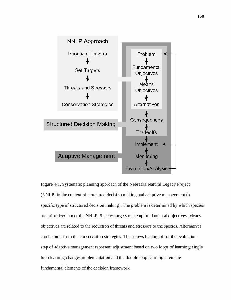
168
Figure 4-1. Systematic planning approach of the Nebraska Natural Legacy Project
(NNLP) in the context of structured decision making and adaptive management (a
specific type of structured decision making). The problem is determined by which species
are prioritized under the NNLP. Species targets make up fundamental objectives. Means
objectives are related to the reduction of threats and stressors to the species. Alternatives
can be built from the conservation strategies. The arrows leading off of the evaluation
step of adaptive management represent adjustment based on two loops of learning; single
loop learning changes implementation and the double loop learning alters the
fundamental elements of the decision framework.

169
Figure 4-2. Dichotomous key for determining when to consider using adaptive
management, given specified uncertainties and knowledge of the management context.
The first part of the key evaluates whether the uncertainty is appropriate for adaptive
management, such that the uncertainty could be reduced through designed monitoring
and review of management consequences. The second part of the key addresses whether
the knowledge gained would be useful. The third part of the key relates to whether it is
practically possible to reduce the uncertainty. Adaptive management is impossible or
unlikely to succeed if the answer to any of these questions is “no.” Potential reasons for
the answer being “no” are listed along the right-hand side of the key.
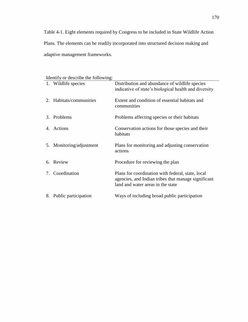
170
Table 4-1. Eight elements required by Congress to be included in State Wildlife Action
Plans. The elements can be readily incorporated into structured decision making and
adaptive management frameworks.
Identify or describe the following:
1. Wildlife species
2. Habitats/communities
3. Problems
4. Actions
5. Monitoring/adjustment
6. Review
7. Coordination
8. Public participation
Distribution and abundance of wildlife species
indicative of state’s biological health and diversity
Extent and condition of essential habitats and
communities
Problems affecting species or their habitats
Conservation actions for those species and their
habitats
Plans for monitoring and adjusting conservation
actions
Procedure for reviewing the plan
Plans for coordination with federal, state, local
agencies, and Indian tribes that manage significant
land and water areas in the state
Ways of including broad public participation
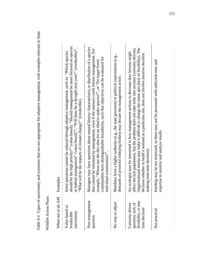
171
Tab
le 4
-2.
Types
of
unce
rtai
nty
and s
cen
ario
s th
at a
re n
ot
app
ropri
ate
for
adap
tive
man
agem
ent,
wit
h e
xam
ple
s re
levan
t to
Sta
te
Wil
dli
fe A
ctio
n P
lans.
When
not
to d
o A
M
Ex
ample
s
Val
ue-
bas
ed o
r
irre
duci
ble
unce
rtai
nty
Som
e ques
tions
cannot
be
reduce
d t
hro
ugh a
dap
tive
man
agem
ent,
such
as:
“W
hic
h s
pec
ies
should
be
the
hig
h p
riori
ty?”
(val
ue-
bas
ed),
“S
hou
ld m
anag
emen
t be
more
focu
sed o
n s
pec
ies
or
hab
itat
man
agem
ent”
(val
ue-
bas
ed)?
”, “
Wil
l th
ere
be
a d
rou
ght
nex
t yea
r?”
(irr
educi
ble
)”,
“What
wil
l be
the
impac
ts o
f cl
imat
e ch
ange?
” (i
rred
uci
ble
).
No
n-m
anag
emen
t
ques
tion
Man
ager
s m
ay h
ave
qu
esti
ons
about
nat
ura
l his
tory
ch
arac
teri
stic
s o
r d
istr
ibu
tio
n o
f a
spec
ies
that
can
not
be
info
rmed
by m
anag
emen
t, e
ven
if
the
answ
ers
could
info
rm m
anag
emen
t. F
or
exam
ple
, “W
her
e ar
e th
e den
sit
es f
or
an e
lusi
ve
snak
e sp
ecie
s?”,
or
“Do t
arget
fore
st
com
munit
ies
hav
e dis
tinguis
hab
le b
ound
arie
s, s
uch
that
obje
ctiv
es c
an b
e ev
aluat
ed f
or
indiv
idual
co
mm
unit
ies?
”.
No w
ay t
o a
dju
st
Man
dat
es f
rom
a h
igh
er a
uth
ori
ty (
e.g., t
he
stat
e gover
nor)
or
poli
tica
l ex
pec
tati
ons
(e.g
.,
dem
ands
of
pow
erfu
l lo
bb
yin
g b
odie
s) m
ay d
icta
te t
he
man
agem
ent
acti
on.
Curi
osi
ty-d
riven
ques
tion, la
ck o
f
flex
ibil
ity, o
r one-
tim
e dec
isio
n
An e
colo
gis
t m
ay b
e in
tere
sted
in h
ow
man
agem
ent
acti
ons
to d
ecre
ase
dee
r bro
wse
mig
ht
affe
ct t
he
tick
popula
tion, but
the
pro
ble
m d
oes
no
t ta
ke
tick
s in
to a
ccount
(curi
osi
ty-d
riven
).
Org
aniz
atio
nal
iner
tia
may
mak
e it
dif
ficu
lt t
o c
han
ge
the
stat
us
quo (
lack
of
flex
ibil
ity).
Th
e
dec
isio
n w
het
her
to b
uil
d a
wet
land a
t a
par
ticu
lar
site
, does
not
involv
e it
erat
ive
dec
isio
n
mak
ing (
on
e-ti
me
dec
isio
n).
Not
pra
ctic
al
Fundin
g m
ay b
e to
o r
estr
icte
d, or
ther
e m
ay n
ot
be
per
sonnel
wit
h s
uff
icie
nt
tim
e an
d
exper
tise
to m
onit
or
and a
nal
yze
res
ult
s

172
Tab
le 4
-3. A
spec
ts o
f ad
apti
ve
man
agem
ent
(AM
) pro
ject
des
ign w
ith e
xam
ple
s re
levan
t to
Sta
te W
ildli
fe A
ctio
n P
lans.
How
to d
esig
n
AM
E
xam
ple
s
Involv
e th
e
righ
t p
eop
le
If a
wel
l-re
spec
ted r
anch
er a
gre
es t
o w
ork
wit
h a
sta
te b
iolo
gis
t to
ex
per
imen
t w
ith t
echniq
ues
for
reduci
ng
wood
y e
ncr
oac
hm
ent,
oth
er c
om
munit
y m
emb
ers
may
bec
om
e in
tere
sted
. C
on
ver
sely
, if
th
e sa
me
ran
cher
feel
s al
ien
ated
or
that
his
opin
ions
are
under
val
ued, he
may d
issu
ade
oth
ers
from
bec
om
ing i
nvolv
ed.
Pri
ori
tize
unce
rtai
nti
es
In a
n a
gri
cult
ure
-support
ed c
om
munit
y, a
targ
et s
pec
ies
dep
end
s on w
etla
nds.
Tw
o u
nce
rtai
nti
es e
mer
ge
duri
ng
pla
nnin
g:
(1)
agro
chem
ical
s im
pac
ts a
nd (
2)
bes
t m
ethods
for
wet
land c
on
stru
ctio
n. W
rong a
ssum
pti
on
s ab
out
the
amount
of
tole
rable
agro
chem
ical
s co
uld
lea
d t
o t
erri
ble
conse
qu
ence
s fo
r th
e sp
ecie
s, s
takeh
old
ers,
or
both
. C
onst
ruct
ing s
ubpar
wet
lands
is l
ess
risk
y t
han
mis
regula
ting c
hem
ical
s an
d e
xper
imen
t co
sts
outw
eigh
pro
ject
ed b
enef
its.
Ther
efore
, th
e ag
roch
emic
al u
nce
rtai
nty
should
be
pri
ori
tize
d.
Rep
rese
nt
hypoth
eses
wit
h m
odel
s
In a
fir
e-ad
apte
d o
ak f
ore
st, th
ere
may b
e dif
fere
nt
hypoth
eses
about
the
impac
ts o
f fi
re f
requen
cy a
nd i
nte
nsi
ty
on o
ak r
egen
erat
ion a
nd t
he
import
ance
of
envir
on
men
tal
fact
ors
, su
ch a
s li
ght
avai
labil
ity. M
ult
iple
model
s
wit
h d
iffe
rent
var
iable
s an
d r
elat
ionsh
ips
can b
e d
evel
oped
and u
sed t
o p
redic
t oak
reg
ener
atio
n f
oll
ow
ing f
ire
man
agem
ent.
Choose
how
to
lear
n
An N
GO
wan
ts t
o t
est
bis
on
gra
zing a
s a
pra
irie
man
agem
ent
tool.
Ther
e is
unce
rtai
nty
about
how
man
y b
ison
can b
e su
pport
ed e
colo
gic
ally
and e
conom
ical
ly.
Act
ive
adap
tive
man
agem
ent
would
div
ide
the
pra
irie
into
unit
s an
d t
est
dif
fere
nt
trea
tmen
ts. S
om
e ar
eas
may
be
dam
aged
or
money c
ould
be
lost
, but
lear
nin
g w
ould
be
rela
tivel
y q
uic
k. A
pas
siv
e ap
pro
ach w
ould
gen
erat
e dif
fere
nt
model
-bas
ed p
redic
tions,
im
ple
men
t th
e
hypoth
esiz
ed o
pti
mal
tre
atm
ent,
and c
om
par
e re
sult
s to
the
model
s. L
earn
ing i
s sl
ow
er b
ut
safe
r.
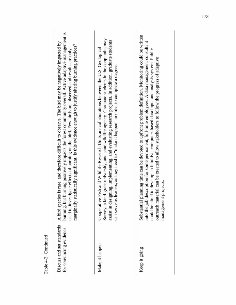
173
Tab
le 4
-3. C
onti
nued
Dis
cuss
and s
et s
tandar
ds
for
convin
cin
g e
vid
ence
A b
ird s
pec
ies
is r
are,
an
d t
her
efore
dif
ficu
lt t
o o
bse
rve.
The
bir
d m
ay b
e n
egat
ivel
y i
mp
acte
d b
y
burn
ing, but
burn
ing p
osi
tivel
y i
mpac
ts t
he
fore
st c
om
munit
y o
ver
all.
Act
ive
adap
tive
man
agem
ent
is
use
d t
o i
nves
tigat
e ef
fect
s of
burn
ing o
n t
he
bir
d.
Few
bir
ds
are
obse
rved
and r
esult
s ar
e only
mar
gin
ally
sta
tist
ical
ly s
ignif
ican
t. I
s th
is e
vid
ence
enou
gh t
o j
ust
ify a
lter
ing b
urn
ing p
ract
ices
?
Mak
e it
hap
pen
C
ooper
ativ
e F
ish a
nd W
ildli
fe R
esea
rch U
nit
s ar
e co
llab
ora
tion
s bet
wee
n t
he
U.S
. G
eolo
gic
al
Surv
ey,
a la
nd-g
rant
univ
ersi
ty,
and s
tate
wil
dli
fe a
gen
cy. G
rad
uat
e st
ud
ents
in
th
e co
op
un
its
may
assi
st i
n d
esig
nin
g, im
ple
men
ting, an
d e
val
uat
ing r
esea
rch p
roje
cts.
In a
ddit
ion, gra
duat
e st
uden
ts
can s
erv
e as
lea
der
s, a
s th
ey n
eed t
o “
mak
e it
hap
pen
” in
ord
er t
o c
om
ple
te a
deg
ree.
Kee
p i
t goin
g
Subst
anti
al p
lannin
g t
ime
can b
e d
evote
d t
o u
pfr
on
t pro
ble
m d
efin
itio
n. M
onit
ori
ng c
ould
be
wri
tten
into
the
job d
escr
ipti
on f
or
som
e per
man
ent,
full
-tim
e em
plo
yee
s. A
dat
a m
anag
emen
t co
nsu
ltan
t
could
be
hir
ed t
o d
evel
op a
n i
ntu
itiv
e, c
om
pute
r-b
ased
dat
a in
put
and a
nal
ysi
s sy
stem
. P
ubli
c
outr
each
mat
eria
l ca
n b
e cr
eate
d t
o a
llow
sta
keh
old
ers
to f
oll
ow
the
pro
gre
ss o
f ad
apti
ve
man
agem
ent
pro
ject
s.
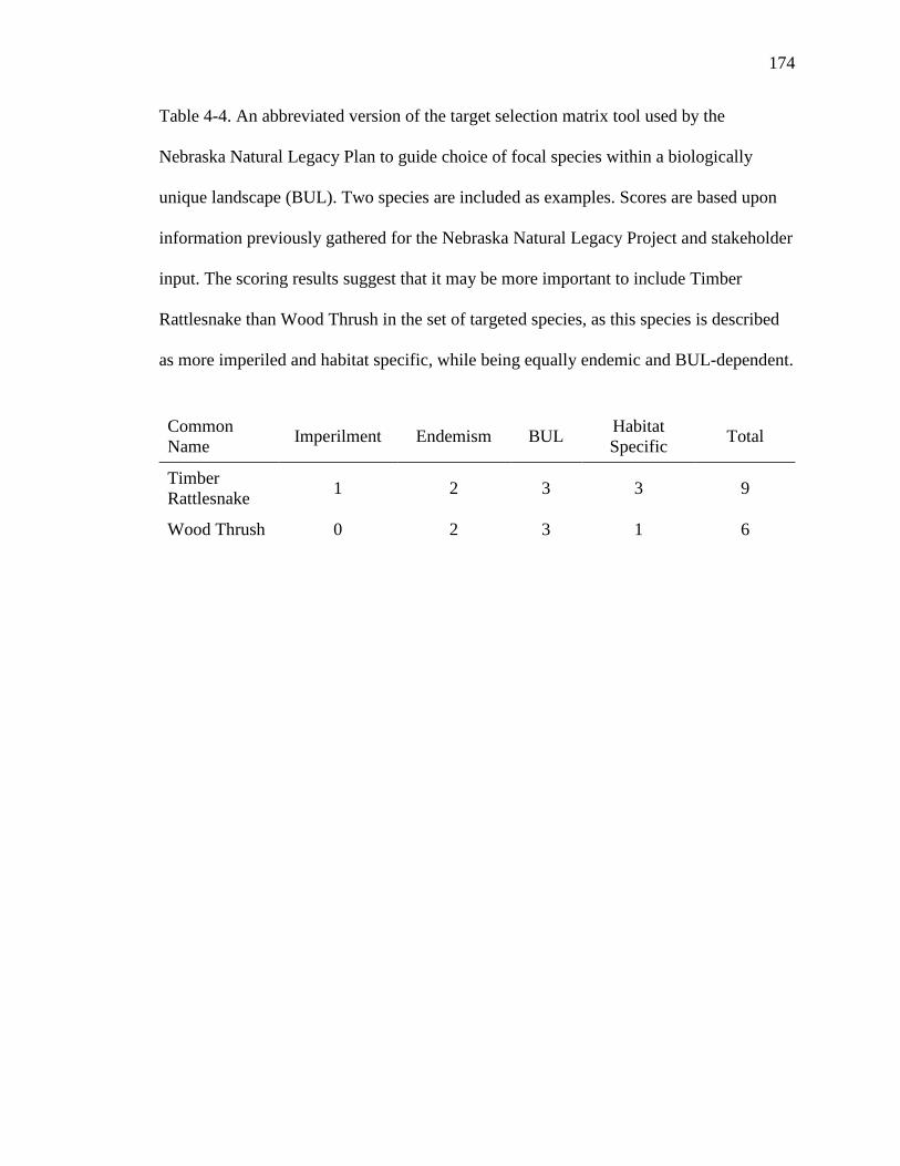
174
Table 4-4. An abbreviated version of the target selection matrix tool used by the
Nebraska Natural Legacy Plan to guide choice of focal species within a biologically
unique landscape (BUL). Two species are included as examples. Scores are based upon
information previously gathered for the Nebraska Natural Legacy Project and stakeholder
input. The scoring results suggest that it may be more important to include Timber
Rattlesnake than Wood Thrush in the set of targeted species, as this species is described
as more imperiled and habitat specific, while being equally endemic and BUL-dependent.
Common
Name Imperilment Endemism BUL
Habitat
Specific Total
Timber
Rattlesnake 1 2 3 3 9
Wood Thrush 0 2 3 1 6
175
CHAPTER 5: REDUCING UNCERTAINTY ABOUT OAK SEEDLING
ABUNDANCE TO IMPROVE CONSERVATION OF OAK-DOMINATED FORESTS
1. INTRODUCTION
Oak-dominated forests are valued for many reasons, including supporting
wildlife, supplying timber, and providing cultural benefits (Fei et al. 2011). Ecologist and
forest managers have observed a general trend of reduced oak abundance in eastern North
America since the 1980’s (Abrams 1992, Fei et al. 2011). Loss of fire on the landscape is
believed to be a major driver of the oak decline. In the absence of fire, more shade-
tolerant but less fire-tolerant tree species a competitive advantage over oaks by reducing
light availability to oak seedlings (Nowacki and Abrams 2008). Therefore, prescribed
burning and thinning of shade-tolerant trees may be necessary to conserve oak-dominated
ecosystems.
Studies have examined the general impacts of burning and thinning (Iverson et al.
2008, Abrams and Steiner 2013, Knapp et al. 2015), but the consequences for a given oak
forest will likely depend on the historical context, present condition, and how burning
and thinning are applied. Adaptive management is a useful framework for learning about
specific forest systems by testing different hypotheses about consequences through
monitoring and review (Holling 1978, Walters 1986, Lyons et al. 2008, Williams et al.
2009). Adaptive management is appropriate when there is: (a) uncertainty about how
systems or species might respond to management or uncertainty about the particular
mechanisms driving observed responses (Williams et al. 2009), (b) an ability to learn, and
176
(c) opportunity to change management based on what is learned (Williams and Brown
2012).
One area of uncertainty related to oak conservation management is the impact
burning and thinning will have on oak seedling abundance. Assuming that seedling
abundance is indicative of oak regeneration potential, reducing uncertainty about oak
seedling abundance through adaptive management can improve oak conservation.
Hypotheses (i.e., models) could differ based on management specifics (e.g., frequency
and intensity of prescribed burning, amount of thinning), predicted shape of the response
(e.g., positive vs. negative, linear vs. nonlinear), strength (i.e., coefficients) of anticipated
effect, or the potential for interactions between management actions (e.g., whether the
impact of burning is different in the presence of thinning; whether thinning is effective
without burning). In order to detect the management effects, variability resulting from
environmental drivers will likely need to be accounted for in the models.
To conserve and restore oak-dominated forest communities as part of Nebraska’s
State Wildlife Action Plan, also known as the Nebraska Natural Legacy Project
(Schneider et al. 2011), managers have reintroduced fire at Indian Cave State Park in
southeastern Nebraska, in conjunction with thinning of small trees. Management
practices can be informed by similar oak conservation efforts elsewhere in the Midwest
(e.g., Iverson et al. (2008) found that repeated burning and partial thinning in a southern
Ohio forest increased the density of large oak seedlings, and Knapp et al. (2015) found
that after 60 years, areas with repeated burning on a four-year fire interval contained
more oak seedlings than unburned areas). However, uncertainties remain about how the
177
oak forest communities of southeastern Nebraska will respond, including how
management will impact oak seedling abundance.
Previously adaptive management was not possible at Indian Cave State Park
because a lack of data prevented formal evaluation of management. As an initial step
toward reducing uncertainty through adaptive management, a series of meetings with
park managers and state conservation planners was used to develop hypotheses about the
environmental and management factors influencing oak seedling abundance and to design
data collection methods for an initial inventory of oak seedlings at Indian Cave State
Park. In this chapter, I use the inventory data to test hypotheses built from combinations
of various environmental drivers and management actions through a multimodel
inference/information theoretic approach. I also explore opportunities for further
implementing adaptive management, built upon the knowledge acquired from this
preliminary effort.
2. STUDY SITE AND DATA COLLECTION
Indian Cave State Park is an approximately 3,300-acre parcel of state protected
land in the Missouri River bluffs of southeastern Nebraska (Schneider et al. 2011). The
park contains mixed hardwood forest communities dominated by red and white oaks,
hickories, and basswood. Based on familiarity with oak conservation practices elsewhere,
park managers hypothesize that burning creates suitable conditions for oak seedling
germination and thinning improves oak seedling survival by increasing light availability.
Prescribed burning was first applied in the park in 2009, and since then prescribed
178
burning and thinning have been applied in sections of the park. Management was not
conducted as a formal experimental procedure but rather implemented opportunistically.
Data were collected during the months of June and July 2014. The oak seedling
inventory was conducted in tandem with a broader Indian Cave State Park forest
community inventory project (unpublished data). A total of 360 points were located
throughout the forested areas of the park, using stratified random sampling to collect data
from 30 points in each of 12 elevation/aspect combinations; presence of oak communities
can be driven by elevation and aspect (Collins and Carson 2004). At each of the points,
canopy closure, understory plant groundcover, litter:bare groundcover, oak seedling
abundance, and tree composition was assessed.
Canopy closure was estimated at each point using a spherical densiometer, with
readings averaged between two observers when possible. Within a 4-m radius plot
centered on the point, the percentage of ground covered by plants less than 6-ft tall was
visually estimated, as was the percentage of litter to bare ground (summed to 100%). In
the same plot, oak seedlings were counted and distinguished as red or white oak seedlings
to the best of the observers’ abilities. Within a 10-m radius plot, all trees (greater than 6-ft
tall) were recorded to species, assigned a size class based on diameter at breast height
(dbh) (small: ≤ 10-cm dbh, medium: 10-cm < dbh < 30-cm, large: ≥ 30-cm dbh), and
designated canopy or subcanopy (where a canopy tree is defined as receiving direct
overhead sunlight). A geographic information systems layer of the park, provided by a
manager, was used to determine if points were within 20-m of an opening (edge).
3. RESPONSE VARIABLE AND COVARIATES
179
The response variable of interest for this study is oak seedling abundance. Red
and white oak seedlings are combined to avoid numerous zero values and due to
uncertainty about the accuracy of differentiation between red and white oak groups. The
covariates, selected based on meetings with park managers and state conservation
planners, include a mix of ecological and management variables to explore the factors
correlated with oak seedling abundance and to test for evidence of management effects.
The covariates are: number of large oaks within 10-m, number of small trees (any
species) within 10-m, number of times burned (based on management burn units),
number of times burned before mid-2012 (prior to germination following a mast year),
and edge (y/n). Canopy closure was excluded from the present study based on the limited
range observed in the park (75% of points with canopy closure over 90% and only
outliers below 80% closure) and unsupportive results from a pilot study conducted the
previous summer (unpublished data).
Large oaks, in comparison to medium and small oaks, have greater basal area for
acorn production and tend to produce more acorns per basal area (Greenberg 2000).
Many of those acorns settle near their source tree (Sork 1984, Dow and Ashley 1996). In
addition, if the environmental conditions at the site (e.g., elevation and aspect, soil
moisture) are favorable to large oaks, they may be suitable for seedlings as well, although
this is not necessarily the case and may be species specific (Collins and Carson 2004).
Therefore, greater numbers of large oaks are hypothesized to increase the number of
seedlings. Analysis of a pilot study (30 points collected in 2013) further supports
inclusion of large oaks as a covariate.
180
Thinning has been implemented in areas of the park in an effort to reduce the
number of small, shade-tolerant trees. Fewer small trees are hypothesized to increase the
number of seedlings by allowing greater light availability. Due to lack of sites that were
thinned and not burned, and given the variability in the number of small trees remaining
at thinned sites, the number of small trees is used as a surrogate for thinning.
The impact of burning is hypothesized to be influenced by how often a site was
burned and whether burning occurred prior to or post the late spring 2012 germination of
seedlings produced in the mast of fall 2011. Managers assume that most of the seedlings
observed during the study are from the spring 2012 cohort. Fire before the late spring
2012 germination (hereafter pre-germination) is hypothesized to have increased oak
seedling abundance by providing suitable germination conditions. The impact of fire post
germination is less well understood. Pre-germination, sites were burned zero, one, two, or
four times. Given a strong relationship between the number of times burned pre- and
post- germination (Table 5-1), the number of times burned post-germination is not as a
covariate; instead, models include “number of times burned total” or “number of times
burned pre-germination.” For the analysis, number of times burned is modeled as a
factor, rather than a count variable, to accommodate potential threshold effects.
There are many ways in which edge could influence seedling counts. Sites near
the edge could receive more sunlight and increase the number of seedlings, or edge sites
could experience greater human disturbance and decrease the number of seedlings. A
model with edge was included to test whether there was evidence of an edge effect. Edge
was treated as a binary variable, where “1” indicates a point is within 20-m of an
181
opening, and “0” indicates a point is more than 20-m from an opening (determined using
an available GIS data layer).
4. STATISTICAL METHODS
Prior to selecting the models to compare, covariates were tested for collinearity to
avoid inclusion of correlated covariates in the same model, as this can generate confusing
results (Zuur et al. 2010). The set of models represents hypotheses about what
environmental drivers and management actions impact oak seedling abundance (Table 5-
2). Most models contain additive covariates, but an interaction between small trees and
burning was included to address a specific hypothesis that the relationship between
burning and oak seedling abundance may be impacted by the number of small trees
present. Each model was fit to the sample data using a negative binomial family
distribution, implemented in R (version 3.1.0, 2014) with glm.nb in package MASS
(Venables and Ripley 2002). The negative binomial family was chosen to address
overdispersion discovered during data exploration under a Poisson distribution.
Following the multimodel inference/information theoretic approach to comparing models
(Burnham and Anderson 2002), the AICc (Akaike information criterion, corrected to
address the small sample size), delta AICc, model weights (a.k.a model probabilities),
and cumulative model weights were calculated in R (version 3.1.0, 2014) using package
glmulti (Calcagno and de Mazancourt 2010). Model averaged covariate effect estimates,
average over the full model set (assuming zero effect for models not containing the
covariate) and 95% confidence interval bounds were found using package MuMIn
(Bartoń 2015).
182
5. RESULTS
The number of oak seedlings within the 4-m radius plots ranged from 0 to 76,
with a mean of 5.33 and median of 3. Based on the boxplot (Figure 5-1), there are
numerous outliers. The number of large oaks within the 10-m plots ranged from 0 to 14
trees, with a mean of 2.97 and median of 2. Based on the boxplot (Figure 5-2), there are
two potential outliers. The number of small trees ranged from 0 to 101, with a mean of
19.47 and median of 15. The boxplot (Figure 5-3) suggests a number of potential outliers.
Of the 360 points, 47 were designated edge (313 not edge). All outliers were retained but
may have influenced the results.
The two quantitative covariates, number of large oaks and number of small trees,
were not strongly correlated (r = 0.17) (Figure 5-4). Relationships with and between
categorical variables (Figure 5-5) were examined with Poisson generalized linear
modeling for count data and binomial modeling for the edge data. Statistically significant
effects were detected in most cases (Table 5-3) but because of the relevancy to
management and the relatively small size of effects, these covariates were allowed to
appear in the same models, acknowledging that this may influence model results.
The top model is “oak seedling abundance ~ number of large oaks” with a weight
of 0.33 (Table 5-2, Figure 5-6) 11. The next closest model is “oak seedling ~ large oaks +
times burned pre-germination” with a delta AICc of 1.03 and weight of 0.20. Of the 17
models, eight have a weight greater than 0.005, all of which contain the number of large
11 Model averaging was deemed unnecessary for the purposes of displaying the relationship between large
oaks and oak seedling abundance because the coefficient for large oaks did not vary widely between
models containing large oaks (ranging from 0.165 to 0.177).

183
oaks. Model averaged covariate effect estimates result in the number of large oaks being
the only covariate (ignoring the intercept) with a 95% confidence interval not containing
0 (Table 5-4).
6. DISCUSSION
The results support the hypothesis that the number of large oaks influences the
number of oak seedlings. The top model contains this covariate alone, all the models with
weight greater than 0.005 include large oaks, and the 95% confidence interval excludes 0
for the model averaged effect estimate. The finding that the number of large oaks is
correlated with oak seedling abundance is supported by the results of Collins and Carson
(2004).
Unlike other studies (e.g., Iverson et al. 2008, Abrams and Steiner 2013, Knapp et
al. 2015), management effects were not detected. Although the covariates for times
burned pre-germination and the number of small trees appear in the second and third best
models, respectively, the models also contain the number of large oaks and are less
supported than the model with large oaks alone. This suggests that these covariates likely
do not substantially help explain the variability.
Lack of evidence does not necessarily mean that management is failing. Other
possible explanations include: (a) management needs more time to make an observable
impact, (b) there were too few data points to detect differences, (c) the relationships
between covariates or outliers influenced the results, or (d) another covariate could be
driving the effectiveness of management, such that the impacts of management cannot be
detected without accounting for the covariate. Other environmental factors that were not

184
considered in this analysis include soil conditions, groundcover of different types of
understory vegetation (e.g., nettles, hog peanut, sunflower), and detailed topographical
characteristics (e.g., degree of slope, drainages). Adaptive management could further
resolve uncertainties about environmental drivers and management impacts.
7. ADAPTIVE MANAGEMENT POTENTIAL
The Nebraska Natural Legacy Project encourages the use of adaptive management
to reduce uncertainty about how systems in Nebraska work, for the purposes of
improving conservation of wildlife and their habitats (Schneider et al. 2011). The models
representing different hypotheses about which factors are related to oak seedling
abundance, demonstrate uncertainty prior to the study. The results, particularly the
relatively low weight (0.33) of the top model (oak seedling abundance ~ number of large
oaks), show that substantial uncertainty remains about the drivers of oak seedling
abundance.
As management decisions were not made with learning in mind, the present study
is closer to external research than adaptive management. However, the study could
inform an adaptive management approach (William 2015), especially the establishment
of management hypotheses and baseline data that can be used for future comparisons. It
may be worth developing an active adaptive management approach, in which learning is
an objective driving management decisions. Indian Cave State Park is an ideal, and
perhaps the only feasible, setting for experimenting with methods for oak conservation in
southeastern Nebraska. The park covers a relatively large area (approximately 3,300
acres), contains a sizeable portion of the oak-dominated forestland in the state (within
185
Nebraska these natural communities only occur along the Missouri river bluffs on the
eastern state border), is supported by state agency (in contrast to private) resources, and
has managers experienced with prescribed burning and thinning.
The adaptive management project could use plots established within the park to
test different management strategies, such as doing nothing, burning, thinning, and
burning with thinning. Although some of these strategies are unlikely to improve oak
conservation, such as doing nothing, testing the extremes of management alternatives can
increase the probability of detecting an effect, and thus speed the rate of learning.
Another way to improve the chances of detecting an effect is to limit variability between
plots. For example, the study shows that the number of large oaks has an impact on the
number of seedlings. Accounting for this variability could mean identifying sites with
similar numbers of large oaks or controlling the number of seedlings by planting
seedlings.
8. CONCLUSION
The results of this study highlight the importance of accounting for the number of
large oaks in models of oak seedling abundance. While it does not provide evidence that
management efforts to date have influenced seedling abundance, this does not mean that
management is failing to improve oak forest condition. Given the uncertainty remaining
after the preliminary analysis, adaptive management may be appropriate. Although
adaptive management requires substantial planning and resources for implementation, the
ultimate success of management may depend on learning how to improve the
effectiveness of conservation efforts. Indian Cave State Park is perhaps the best place to
186
try an adaptive management approach to oak conservation in southeastern Nebraska
under the Nebraska Natural Legacy Project. Our study provides a starting point for
implementing adaptive management by having already included managers and
conservation planners in the process, developed a monitoring protocol, modeled multiple
management hypotheses, and provided baseline data for comparisons over time.
9. LITURATURE CITED
Abrams, M. D. 1992. Fire and the development of oak forests. BioScience 42:346–353.
Abrams, M. D. and K.C. Steiner. 2013. Long-term seedling height growth and
compositional changes following logging and wildfire in a central Pennsylvania oak
forest. Castanea 78:256–265.
Bartoń, K. 2015. MuMIn: Multi-model inference – model selection and model averaging
based on information critera. R package version 1.14.0
Burnham K.P. and D. R. Anderson 2002. Model selection and multimodel inference: a
practical information-theoretic approach, 2nd edition. Springer, New York, NY.
Calcagno, V. and C. de Mazancourt. 2010. glmulti: an R package for easy automated
model selection with (generalized) linear models. Journal of Statistical Software
34(12):1–29.
Collins, B. and L. L. Battaglia. 2008. Oak regeneration in southeastern bottomland
hardwood forest. Forest Ecology and Management 255:3026–3034.
Collins, R. J. and W. P. Carson. 2004. The effects of environment and life stage on
Quercus abundance in the eastern deciduous forest, USA: are sapling densities most
responsive to enviornmental gradients? Forest Ecology and Management 201:241–258.
Crow, T. R. 1992. Population dynamics and growth patterns for a cohort of northern red
oak (Quercus rubra) seedlings. Oecologia 91:192–200.
Dow, B. D. and M. V. Ashley. 1996. Microsatellite analysis of seed dispersal and
parentage of saplings in bur oak, Quercus macrocarpa. Molecular Ecology 5:615–627.
Fei, S., N. Kong, K. C. Steiner, W. K. Moser, and E. B. Steiner. 2011. Change in oak
abundance in the eastern United States from 1980 to 2008. Forest Ecology and
Management 262:1370–1377.
187
Greenberg, C. H. 2000. Individual variation in acorn production by five species of
southern Appalachian oaks. Forest Ecology and Management 132:199–210.
Holling, C. S., editor. 1978. Adaptive Environmental Assessment and Management.
Wiley & Sons, New York, NY.
Iverson, L. R., T. F. Hutchinson, A. M. Prasad, and M. P. Peters. 2008. Thinning, fire,
and oak regeneration across a heterogeneous landscape in the eastern U.S.L 7-year
results. Forest Ecology and Management 255:3035–3050.
Knapp, B. O., K. Stephan, and J. A. Hubbart. 2015. Structure and composition of an oak-
hickory forest after over 60 years of repeated prescribed burning in Missouri, U.S.A.
Forest Ecology and Management 344:95–109.
Lyons, J. E., M. C. Runge, H. P. Laskowski, and W. L. Kendall. 2008. Monitoring in the
context of structured decision‐making and adaptive management. The Journal of Wildlife
Management 72:1683–1692.
Nowacki, G. J. and M. D. Abrams. 2008. The demise of fire and “mesophication” of
forests in the eastern United States. BioScience 58:123–138.
R Core Team. 2014. Version 3.1.0. R: A language and environment for statistical
computing. R Foundation for Statistical Computing, Vienna, Austria.
Schneider, R., K. Stoner, G. Steinauer, M. Panella, and M. Humpert. 2011. The Nebraska
Natural Legacy Project: State Wildlife Action Plan. Second edition. The Nebraska Game
and Parks Commission, Lincoln, Nebraska, USA.
Sork, V. L. 1984. Examination of seed dispersal and survival in red oak, Quercus Rubra
(Fagaceae), using metal-tagged acorns. Ecology 65:1020–1022.
Venables, W. N., and B. D. Ripley. 2002. Modern applied statistics with S. 4th edition.
Springer, New York, NY.
Walters, C. J. 1986. Adaptive Management of Renewable Resources. MacMillan
Publishing Company, New York, NY.
Williams, B. K. 2011. Passive and active adaptive management: approaches and an
example. Journal of Environmental Management 92:1371–1378.
Williams, B.K. 2015. Integrating external and internal learning in resource management.
Journal of Wildlife Management 79:148–155.
Williams, B. K., and E. D. Brown. 2012. Adaptive Management: The U.S. Department of
the Interior Applications Guide. Adaptive Management Working Group, U.S.
Department of the Interior, Washington, D.C., USA.

188
Williams, B. K., R. C. Szaro, and C. D. Shapiro. 2009. Adaptive Management: The U.S.
Department of the Interior Technical Guide. Adaptive Management Working Group,
U.S. Department of the Interior, Washington, D.C.
Zuur, A. F., E. N. Ieno, and C. S. Elphick, 2010. A protocol for data exploration to avoid
common statistical problems. Methods in Ecology and Evolution 1: 3–14.

189
Figure 5-1. Boxplot of oak seedling abundance within 4-m radius plot for 360 locations
sampled at Indian Cave State Park in southeastern Nebraska.
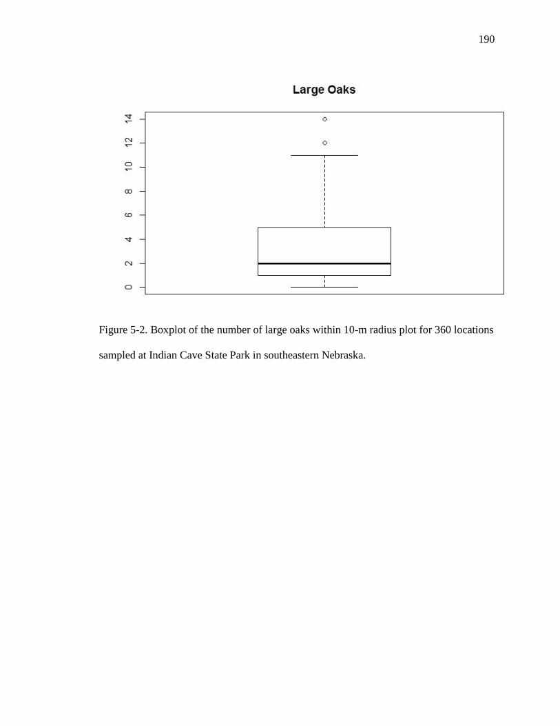
190
Figure 5-2. Boxplot of the number of large oaks within 10-m radius plot for 360 locations
sampled at Indian Cave State Park in southeastern Nebraska.
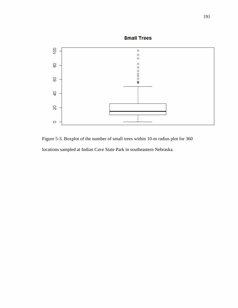
191
Figure 5-3. Boxplot of the number of small trees within 10-m radius plot for 360
locations sampled at Indian Cave State Park in southeastern Nebraska.
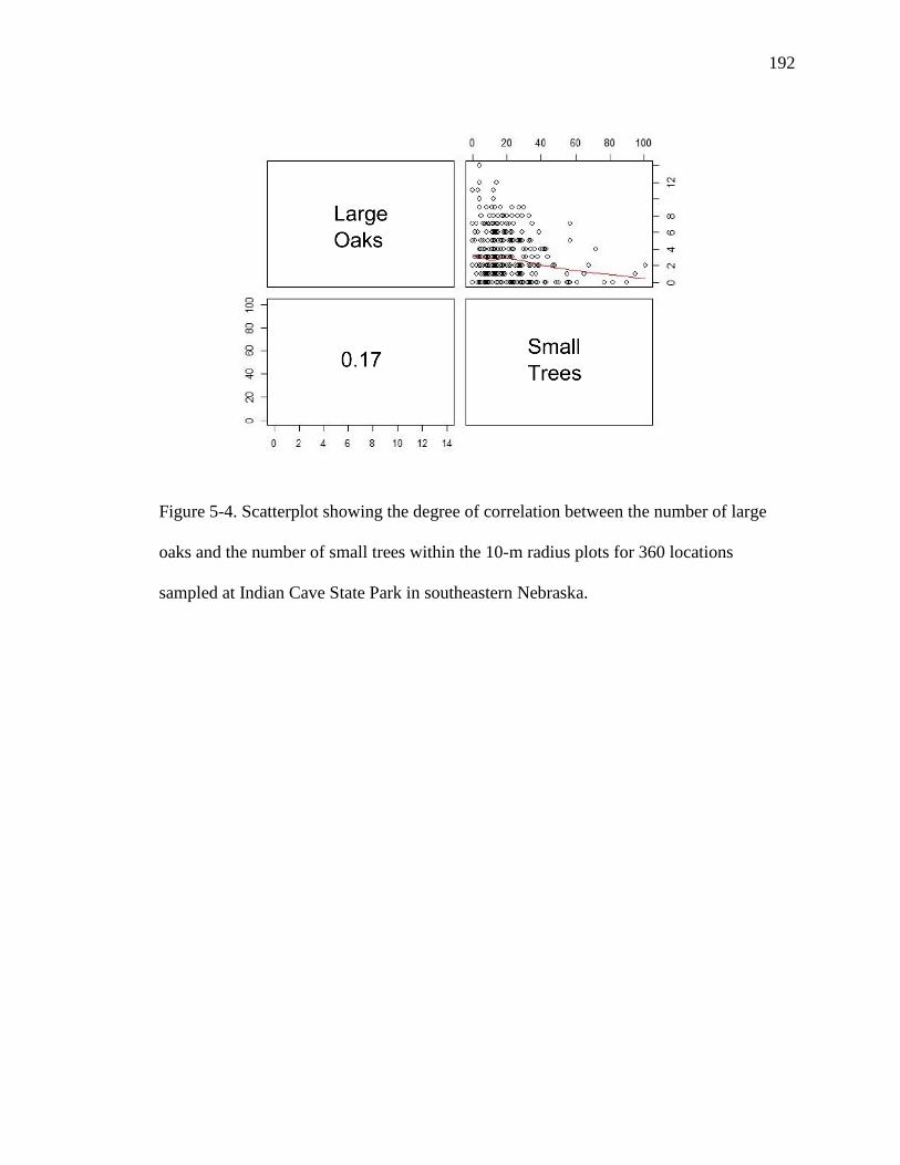
192
Figure 5-4. Scatterplot showing the degree of correlation between the number of large
oaks and the number of small trees within the 10-m radius plots for 360 locations
sampled at Indian Cave State Park in southeastern Nebraska.

193

194
Figure 5-5. Plots of the relationships between the categorical covariates (times burned
pre-germination, total times burned, and edge) and numerical covariates (number of large
oaks, number of small trees). The results suggest that there are potentially important
differences in central tendency and variability when examining covariates in the context
of other covariates, which may impact effect estimates when included together in the oak
seedling abundance models.

195
Figure 5-6. Plot of predicted oak seedling abundance based on the number of large oaks,
using the top model (oak seedling abundance ~ number of large oaks). Dashed lines
indicate the 95% confidence interval. The lines are not straight because the data is back-
transformed from the negative binomial generalized linear model.
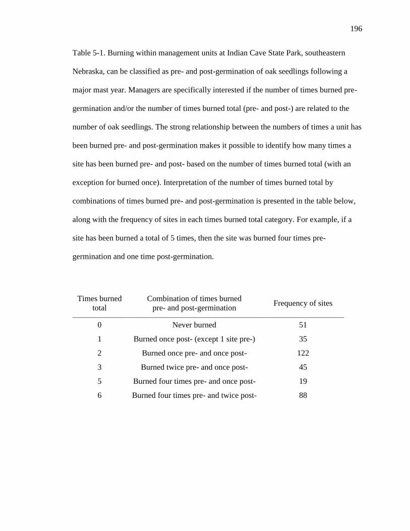
196
Table 5-1. Burning within management units at Indian Cave State Park, southeastern
Nebraska, can be classified as pre- and post-germination of oak seedlings following a
major mast year. Managers are specifically interested if the number of times burned pre-
germination and/or the number of times burned total (pre- and post-) are related to the
number of oak seedlings. The strong relationship between the numbers of times a unit has
been burned pre- and post-germination makes it possible to identify how many times a
site has been burned pre- and post- based on the number of times burned total (with an
exception for burned once). Interpretation of the number of times burned total by
combinations of times burned pre- and post-germination is presented in the table below,
along with the frequency of sites in each times burned total category. For example, if a
site has been burned a total of 5 times, then the site was burned four times pre-
germination and one time post-germination.
Times burned
total
Combination of times burned
pre- and post-germination Frequency of sites
0 Never burned 51
1 Burned once post- (except 1 site pre-) 35
2 Burned once pre- and once post- 122
3 Burned twice pre- and once post- 45
5 Burned four times pre- and once post- 19
6 Burned four times pre- and twice post- 88
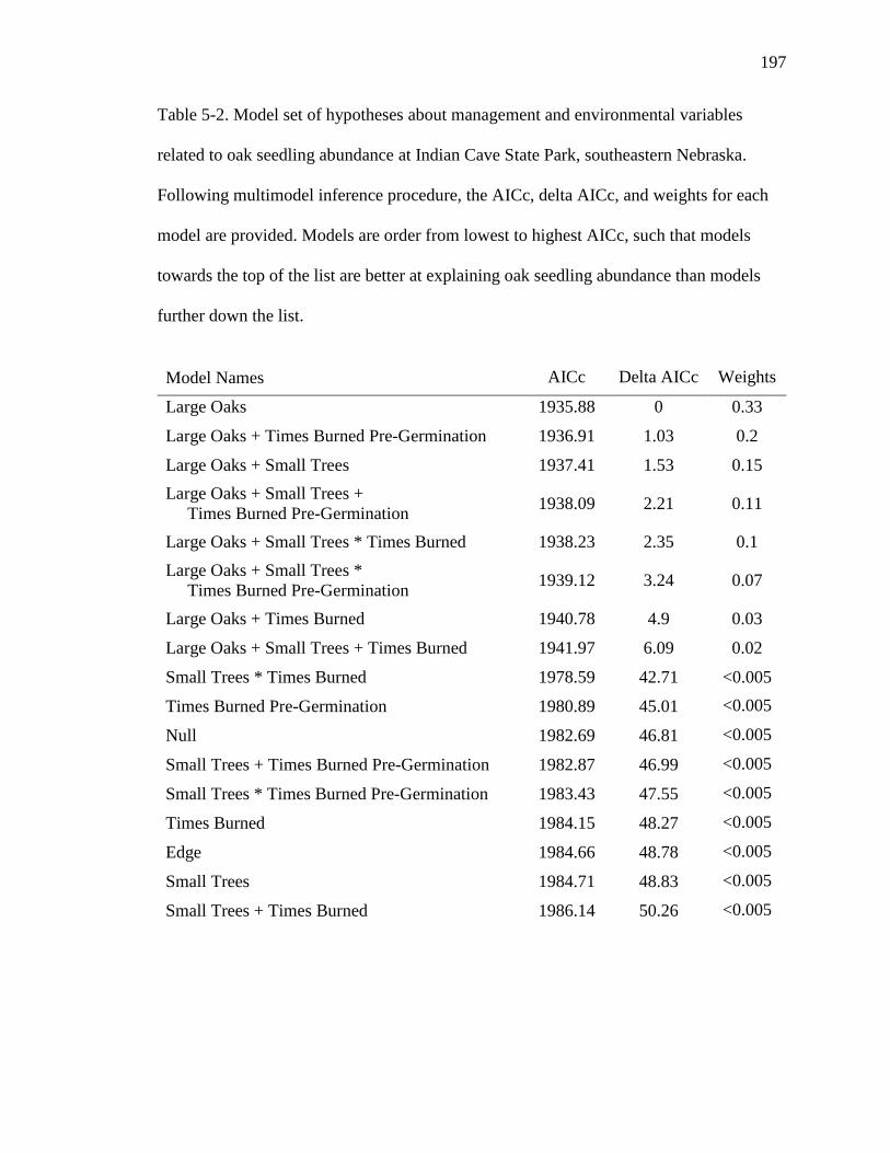
197
Table 5-2. Model set of hypotheses about management and environmental variables
related to oak seedling abundance at Indian Cave State Park, southeastern Nebraska.
Following multimodel inference procedure, the AICc, delta AICc, and weights for each
model are provided. Models are order from lowest to highest AICc, such that models
towards the top of the list are better at explaining oak seedling abundance than models
further down the list.
Model Names AICc Delta AICc Weights
Large Oaks 1935.88 0 0.33
Large Oaks + Times Burned Pre-Germination 1936.91 1.03 0.2
Large Oaks + Small Trees 1937.41 1.53 0.15
Large Oaks + Small Trees +
Times Burned Pre-Germination 1938.09 2.21 0.11
Large Oaks + Small Trees * Times Burned 1938.23 2.35 0.1
Large Oaks + Small Trees *
Times Burned Pre-Germination 1939.12 3.24 0.07
Large Oaks + Times Burned 1940.78 4.9 0.03
Large Oaks + Small Trees + Times Burned 1941.97 6.09 0.02
Small Trees * Times Burned 1978.59 42.71 <0.005
Times Burned Pre-Germination 1980.89 45.01 <0.005
Null 1982.69 46.81 <0.005
Small Trees + Times Burned Pre-Germination 1982.87 46.99 <0.005
Small Trees * Times Burned Pre-Germination 1983.43 47.55 <0.005
Times Burned 1984.15 48.27 <0.005
Edge 1984.66 48.78 <0.005
Small Trees 1984.71 48.83 <0.005
Small Trees + Times Burned 1986.14 50.26 <0.005
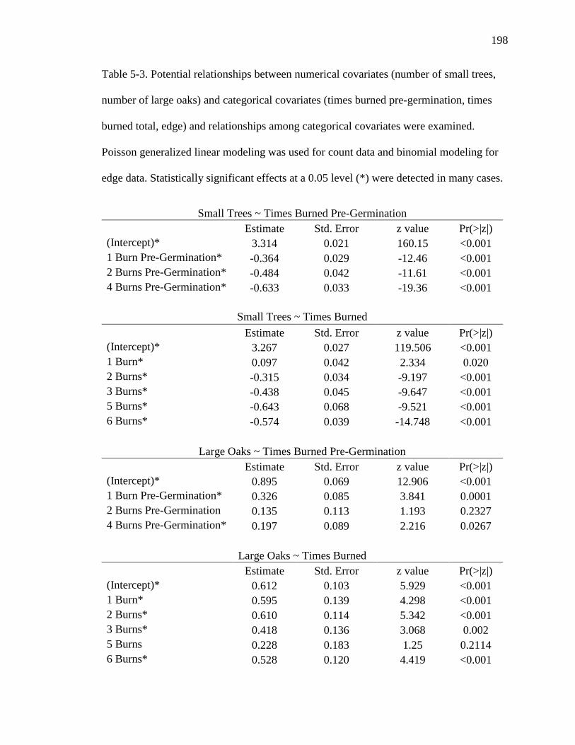
198
Table 5-3. Potential relationships between numerical covariates (number of small trees,
number of large oaks) and categorical covariates (times burned pre-germination, times
burned total, edge) and relationships among categorical covariates were examined.
Poisson generalized linear modeling was used for count data and binomial modeling for
edge data. Statistically significant effects at a 0.05 level (*) were detected in many cases.
Small Trees ~ Times Burned Pre-Germination
Estimate Std. Error z value Pr(>|z|)
(Intercept)* 3.314 0.021 160.15 <0.001
1 Burn Pre-Germination* -0.364 0.029 -12.46 <0.001
2 Burns Pre-Germination* -0.484 0.042 -11.61 <0.001
4 Burns Pre-Germination* -0.633 0.033 -19.36 <0.001
Small Trees ~ Times Burned
Estimate Std. Error z value Pr(>|z|)
(Intercept)* 3.267 0.027 119.506 <0.001
1 Burn* 0.097 0.042 2.334 0.020
2 Burns* -0.315 0.034 -9.197 <0.001
3 Burns* -0.438 0.045 -9.647 <0.001
5 Burns* -0.643 0.068 -9.521 <0.001
6 Burns* -0.574 0.039 -14.748 <0.001
Large Oaks ~ Times Burned Pre-Germination
Estimate Std. Error z value Pr(>|z|)
(Intercept)* 0.895 0.069 12.906 <0.001
1 Burn Pre-Germination* 0.326 0.085 3.841 0.0001
2 Burns Pre-Germination 0.135 0.113 1.193 0.2327
4 Burns Pre-Germination* 0.197 0.089 2.216 0.0267
Large Oaks ~ Times Burned
Estimate Std. Error z value Pr(>|z|)
(Intercept)* 0.612 0.103 5.929 <0.001
1 Burn* 0.595 0.139 4.298 <0.001
2 Burns* 0.610 0.114 5.342 <0.001
3 Burns* 0.418 0.136 3.068 0.002
5 Burns 0.228 0.183 1.25 0.2114
6 Burns* 0.528 0.120 4.419 <0.001
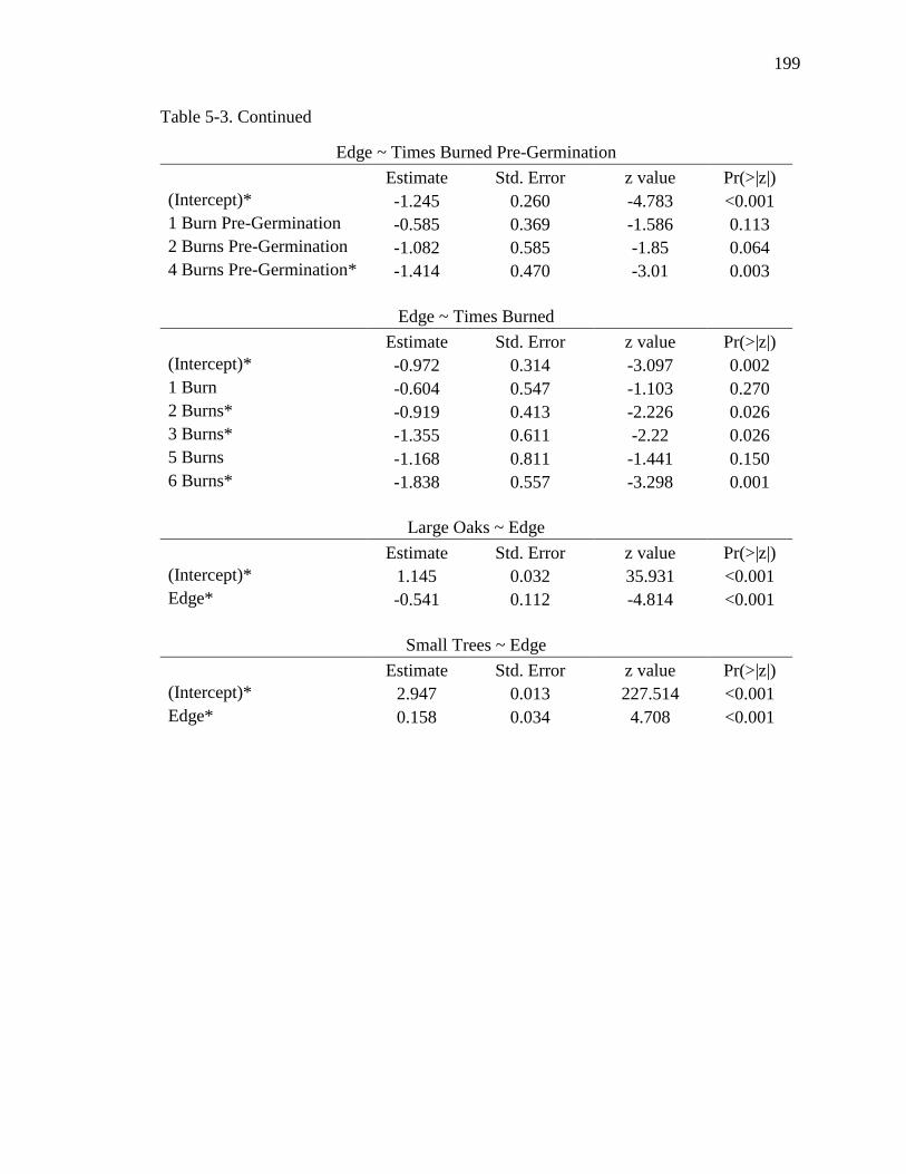
199
Table 5-3. Continued
Edge ~ Times Burned Pre-Germination
Estimate Std. Error z value Pr(>|z|)
(Intercept)* -1.245 0.260 -4.783 <0.001
1 Burn Pre-Germination -0.585 0.369 -1.586 0.113
2 Burns Pre-Germination -1.082 0.585 -1.85 0.064
4 Burns Pre-Germination* -1.414 0.470 -3.01 0.003
Edge ~ Times Burned
Estimate Std. Error z value Pr(>|z|)
(Intercept)* -0.972 0.314 -3.097 0.002
1 Burn -0.604 0.547 -1.103 0.270
2 Burns* -0.919 0.413 -2.226 0.026
3 Burns* -1.355 0.611 -2.22 0.026
5 Burns -1.168 0.811 -1.441 0.150
6 Burns* -1.838 0.557 -3.298 0.001
Large Oaks ~ Edge
Estimate Std. Error z value Pr(>|z|)
(Intercept)* 1.145 0.032 35.931 <0.001
Edge* -0.541 0.112 -4.814 <0.001
Small Trees ~ Edge
Estimate Std. Error z value Pr(>|z|)
(Intercept)* 2.947 0.013 227.514 <0.001
Edge* 0.158 0.034 4.708 <0.001
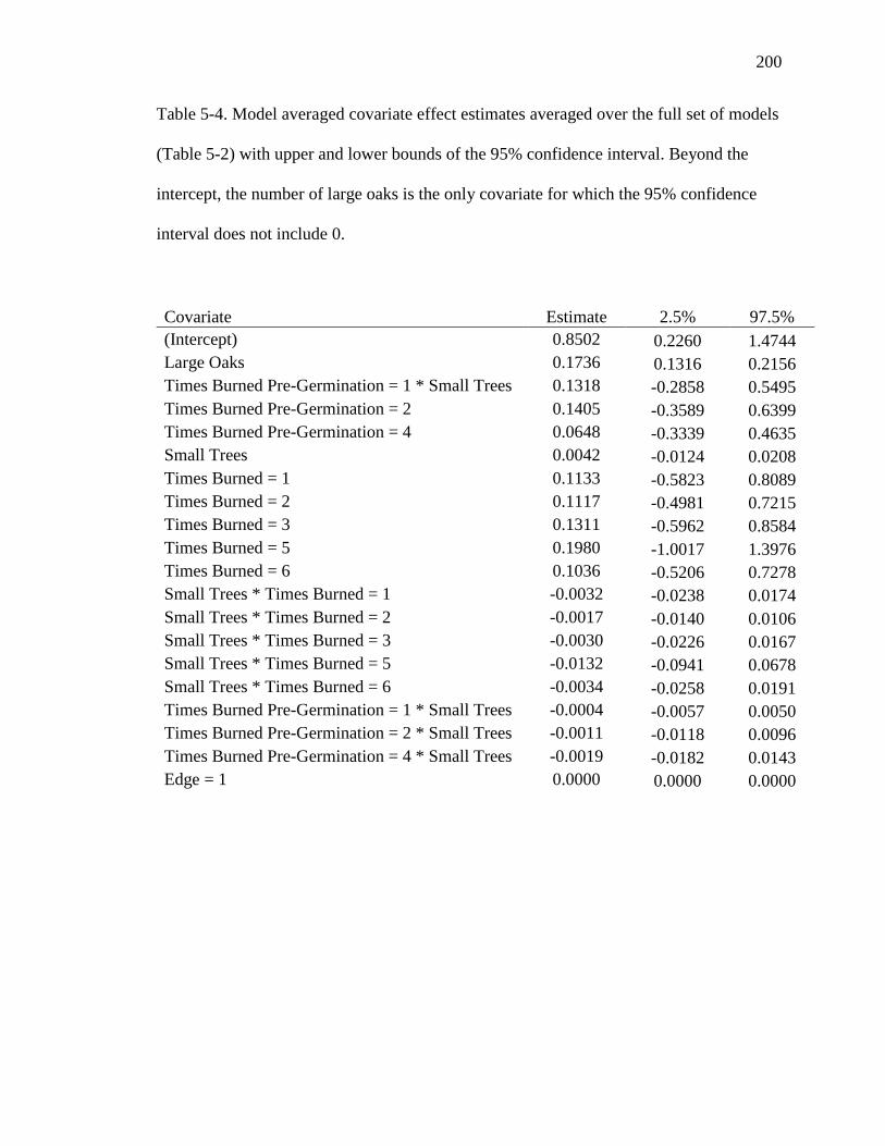
200
Table 5-4. Model averaged covariate effect estimates averaged over the full set of models
(Table 5-2) with upper and lower bounds of the 95% confidence interval. Beyond the
intercept, the number of large oaks is the only covariate for which the 95% confidence
interval does not include 0.
Covariate Estimate 2.5% 97.5%
(Intercept) 0.8502 0.2260 1.4744
Large Oaks 0.1736 0.1316 0.2156
Times Burned Pre-Germination = 1 * Small Trees 0.1318 -0.2858 0.5495
Times Burned Pre-Germination = 2 0.1405 -0.3589 0.6399
Times Burned Pre-Germination = 4 0.0648 -0.3339 0.4635
Small Trees 0.0042 -0.0124 0.0208
Times Burned = 1 0.1133 -0.5823 0.8089
Times Burned = 2 0.1117 -0.4981 0.7215
Times Burned = 3 0.1311 -0.5962 0.8584
Times Burned = 5 0.1980 -1.0017 1.3976
Times Burned = 6 0.1036 -0.5206 0.7278
Small Trees * Times Burned = 1 -0.0032 -0.0238 0.0174
Small Trees * Times Burned = 2 -0.0017 -0.0140 0.0106
Small Trees * Times Burned = 3 -0.0030 -0.0226 0.0167
Small Trees * Times Burned = 5 -0.0132 -0.0941 0.0678
Small Trees * Times Burned = 6 -0.0034 -0.0258 0.0191
Times Burned Pre-Germination = 1 * Small Trees -0.0004 -0.0057 0.0050
Times Burned Pre-Germination = 2 * Small Trees -0.0011 -0.0118 0.0096
Times Burned Pre-Germination = 4 * Small Trees -0.0019 -0.0182 0.0143
Edge = 1 0.0000 0.0000 0.0000
201
CHAPTER 6: CONCLUSION
Uncertainties and conflicting values are prevalent in complex social-ecological
systems and can make it challenging to determine appropriate natural resource
management policies. To help managers proceed in the face of these challenges, a
number of perspectives and tools have been advanced over the past forty years.
Approaches include resilience thinking, structured decision making, adaptive
management, and optimization. Combining the benefits of these various, and inherently
related, management perspectives and tools may further improve our ability to implement
the social-ecological systems paradigm.
Resilience thinking emphasizes the potential for non-linear transitions into
alternative stable states and proposes principles for increasing a social-ecological
system’s capacity to handle disturbances. A structured decision making process can help
managers reach transparent, defensible decisions by articulating problems, incorporating
stakeholder values, describing consequences, and representing uncertainty. Adaptive
management, itself a type of structured decision making, can improve efforts for iterative
decisions by learning through deliberate monitoring, review, and adjustment.
Optimization is a tool for identifying optimal policies for a given characterization of the
system, including system dynamics and objectives.
In this dissertation, I have attempted to link resilience thinking and structured
decision making as a framework for natural resource management, using oak forest
conservation in southeastern Nebraska as a case study. Integrating resilience thinking into
the structured decision making process should generate transparent natural resources

202
management decisions that defensibly account for the lessons of resilience thinking.
Chapter 2 discusses how structured decision making can emphasize principles of
resilience thinking. Chapter 3 demonstrates how optimization can identify policies using
a Markov decision process reflecting elements of resilience thinking. Chapter 4 provides
a practical method for incorporating adaptive management projects into State Wildlife
Action Plans. Chapter 5 presents an initial effort to reduce uncertainty for oak forest
conservation in southeastern Nebraska. In the following sections, I discuss (1)
management implications for oak forest conservation in southeastern Nebraska, (2)
general challenges and limitations that cannot be resolved by incorporating resilience
thinking into structured decision making, (3) methods for improving the framework, and
(4) some concluding remarks.
1. MANAGING INDIAN CAVE STATE PARK
Oak forest conservation is used as a case study throughout the dissertation, with
most chapters specifically discussing management of Indian Cave State Park in
southeastern Nebraska under the Nebraska Natural Legacy Project. I present an example
of how resilience thinking could be incorporated into a structured decision making
process for oak forest management at Indian Cave State Park. I use a Markov decision
process model to depict hypotheses about: (a) the risk of transitioning out the oak-
attracted state, (b) consequences of management actions, and (c) stakeholder values. I
provide a method for identifying questions to address through adaptive management and
outline a potential adaptive management project for Indian Cave State Park. Lastly, I
offer a set of hypotheses related to oak seedling abundance at Indian Cave State Park,

203
identify the number of large oaks as a driver, and suggest ways to further reduce
uncertainty. I now discuss how managers and conservation planners could translate my
recommendations and examples into a realizable management plan for Indian Cave State
Park.
In Chapter 2, I describe hypothetical results of a structured decision making
process that incorporates resilience thinking. In actual application, the problem step
should be expanded by discussing the system history with stakeholders and explicitly
describing what is and is not within control of the group. The objectives should be
selected by the group, being sure to consider general resilience and larger Nebraska
Natural Legacy Project goals. In addition, learning should be considered as an objective,
given the Nebraska Natural Legacy Project’s desire to use adaptive management. The
example set of alternatives is based on previous practices (e.g., prescribed burning and
thinning). Structured decision making encourages creative thinking, so managers should
contemplate whether there are other possibilities. The consequences need to be described
in detail based on the best available information, with uncertainty explicitly represented.
Tradeoffs should be made with a deeper understanding of risk tolerance and the value of
learning.
Decisions about monitoring and review should be made based on the key
uncertainties, the implications of uncertainty, the anticipated value of learning, and a
realistic assessment of the availability of resources. Chapter 4 presents ways of
determining when and how to use adaptive management for State Wildlife Action Plans,
generally, and includes a draft adaptive management plan for Indian Cave State Park. The
example does not explicitly incorporate resilience thinking, but planners could use the
204
information in Chapter 2 to do so. Designing a practical project with a reasonable chance
of success would require: (1) involving the right people (the Nebraska Natural Legacy
Project conservation planners have already established a working group from a subset of
stakeholders), (2) prioritizing uncertainties (which informally occurred by identifying oak
seedling abundance as an important management concern (Chapter 5)), (3) representing
hypotheses with models (discussed shortly), (4) choosing how to learn, (5) setting
standards for convincing evidence, (6) making the project happen (an initial study of oak
seedling abundance has occurred, but further study is needed to determine management
effects), (7) keeping the project going, and (8) deciding when to assess the project.
The Markov decision processes in Chapter 3: (a) represent a quantified resilience-
based state-and-transition model, (b) describe transition probabilities as influenced by
management actions, (c) depict resilience thinking assumptions about the consequences
of specific actions, and (d) incorporate resilience objectives into the reward function.
Optimization was used to help make tradeoffs by determining the state-based policy
expected to achieve the greatest value given probabilities of state transitions, the
desirability of states, and management cost. Planners can use this Markov decision
process optimization approach to determine the specifics for the state-based alternatives
of Chapter 2. Uncertainty about aspects of the Markov decision process can be
incorporated by developing multiple models.
The Markov decision process models of Chapter 3 are highly simplified (e.g., the
reward function does not clearly address all the objectives in Chapter 2) and estimates are
not based on data. For the models to be useful for decision making, the defining
characteristics of each state need to be precisely described, such that it would be possible

205
to designate units as existing in one of the states. The forest inventory data (Chapter 5)
available on tree species composition and size could be used to begin identifying forest
states present on the landscape. In addition, the models must be credible and describe
consequences in terms of the selected objectives and alternatives. Credibility can be
achieved by applying the best available information and having open communication
between experts and decision makers. Communication enables inclusion of the relevant
objectives, alternatives, and consequences, and allows decision makers to make the
necessary value judgments. Chapter 3 highlights the importance of these judgments by
demonstrating sensitivity to model parameters. Given present data limitations for Indian
Cave State Park, models would need to be heavily assumption-based initially, with
multiple models used to represent the range of hypotheses expressed by experts and
decision makers. Monitoring data collected in future surveys could be used to revise
transition probabilities.
In contrast to the Markov decision process models, the models of Chapter 5 relate
to one particular aspect of the oak dominance objective, namely the abundance of oak
seedlings. Instead of describing forest state changes across time, these models explore
what variables (including management actions) are correlated with the number of oak
seedlings for one snapshot in time (seedlings of summer 2014). However, the models can
be used to make assumptions about how the system will change over time (e.g., if
burning was correlated with high numbers of oak seedlings, burning the park should
increase the number of oak seedlings over time and thus increase resilience of the oak-
attracted state). The study of Indian Cave State Park revealed that the number of large
206
oaks is related to oak seedling abundance. Management effects were not detected and
future data collection is needed to elucidate whether management is having an impact.
One important concern is whether there is an ability to conduct monitoring and
subsequently review the data. An initial inventory was conducted (Chapter 5), but
additional monitoring is needed for adaptive management at Indian Cave State Park.
Given sufficient monitoring and review capabilities, the state park is a prime candidate
for an adaptive management project as part of the Nebraska Natural Legacy Project.
Indian Cave State Park contains a large portion of Nebraska’s oak forest communities, is
home to wildlife and plant species targeted by state conservation planners, has
experienced oak forest managers, and has management flexibility. By comparing
observations to predictions made by multiple models (like those of Chapter 3 or Chapter
5), adaptive management could reduce uncertainty about management effects on oak
seedling abundance, or other management-relevant uncertainties. Building from the
structured decision making examples of Chapters 2 and 4, and employing the modeling
approaches of Chapters 3 and 5, Indian Cave State Park managers and conservation
planners can develop an adaptive management plan for maintaining resilience in their oak
forest social-ecological system.
2. GENERAL CHALLENGES AND LIMITATIONS
The framework presented here explores how resilience and structured decision
making (including adaptive management) can be practically applied. However,
implementation will likely still be challenging. Understanding the limitations of the
approach is necessary to establish reasonable expectations about what can be achieved.
207
The framework cannot prevent that: (a) decision making occurs as part of a governance
structure, (b) tough value judgments need to be made, (c) monitoring and review are
difficult, and (d) demonstrating successful increases in resilience (particularly general
resilience) may be impossible.
Structured decision making does not determine the underlying governance
structure, such as who the decision makers are and whether decision makers are
accountable to stakeholders. The governance structured may be predetermined (e.g., set
by federal or state mandates) or may need to be developed (e.g., establishing a group
charter), but in either case this must be done prior to the decision making process.
Dissatisfaction with how the decision will ultimately be made is a source of conflict that
cannot be addressed through the framework.
While structured decision making offers constructive ways of separating conflicts
over values (what people care about) from disagreement about facts (potential actions,
hypothesized consequences), the process does not eliminate the need to make tough
choices about how tradeoffs are made, including how uncertainty and risk are addressed.
For example, managers may have to decide if intensive, costly management is justified if
there is uncertainty about how management is influencing resilience. Choosing what and
how to monitor and review can be especially challenging; on the surface learning while
doing sounds simple and worthwhile, but the realities of resource limitations and
uncertain returns (in terms of how much will actually be learned and whether the
knowledge will influence management practices) can make monitoring and review
difficult to efficiently design and implement.
208
If and how resilience can be measured is a source of debate and has implications
for assessing achievement of a general resilience objective. I avoided the issue by
assuming that the principles of resilience proposed in the literature were sufficient for
assessing general resilience, when used to create sub-objectives as described by
constructed performance measures. This approach is useful for comparing among
alternatives, but does not provide a means for directly observing changes in resilience
over time. Even if an initial decision is reached based on assumptions about the principles
of resilience, debate over the tradeoffs between steady, predictable resource delivery and
natural variability is likely to arise when the project is later assessed for achievement of
objectives.
3. IMPROVING THE FRAMEWORK
Future work is needed to refine and test the framework for synthesizing resilience
thinking and structured decision making in social-ecological systems. One method for
improving the framework would involve asking experts in a particular approach (e.g.,
resilience thinking or decision analysis) to examine the process. The experts would
review whether (a) their approach is accurately represented and (b) the unfamiliar
approaches are understandable. Another method would be to ask natural resources
managers to consider if and how their decision making would be different if they used the
framework. The framework could be tested by conducting workshops. Multiple groups
could go through a given case study using the framework to see where difficulties arise
and how the results differ between groups. Workshops could also be used to compare
decisions and stakeholder satisfaction between frameworks (e.g., structured decision
209
making without resilience thinking; resilience thinking without structured decision
making; ad-hoc decision making) to explore the benefits of applying a particular
approach over another. Ultimately, a framework meant for application must be tested
through implementation. The usefulness of the framework is based on how well it
generates decisions that lead to better natural resources management outcomes than
would have been achieved under traditional decision making approaches.
4. CONCLUDING REMARKS
In the introduction, I argued that we must find ways to transcend the discussion of
the benefits of a complex social-ecological systems paradigm into actually making
informed, defensible decisions under difficult circumstances. I believe developing a
management framework that builds upon structured decision making and explicitly
incorporates resilience thinking is a necessary step toward increasing our ability to
implement the paradigm. To this end, I provide recommendations for the practice of
natural resource management and present ideas that can hopefully foster conversations
between scholars, technical experts, policy makers, and stakeholders regarding how to
address complex management issues. Further progress at the interface of social-
ecological systems theory and natural resource management practice will help us enhance
the resilience of desirable system states, so that we continue to receive ecosystem goods
and services into the distant future.