response of taxonomic groups in streams to gradients in...

Response of taxonomic groups in streams to gradients in

resource and habitat characteristics

Richard K. JohnsonDept. of Aquatic Sciences and Assessment

SLU, Uppsala

What it’s about

• Ecological drivers & scales• Land use & hydro-morphology• Response of stream assemblages to

resource and habitat gradients• Multiple-stressor effects on stream

invertebrates (special thanks to Colin Townsend)

Regional diversity is the result of evolutionary history (rates of speciation and extinction), and sets the upper limit of local diversity.

Geographically distinct regions often have their own distinct flora and fauna…

Inve

rtebr

ate

asse

mbl

ages

Local diversity is constrained by the size of the regional species pool, but often also the size and heterogeneity of the habitat, and the outcome of interactions.

altered after Frissell et al. 1986,Poff 1997 and others

ecoregioncatchmentstreamreachhabitatspace

time

dece

nnia

years

months

days

fishes

plants

inverts

algae

Conceptual models of biological change

hierarchy

envi

ronm

enta

l filt

ers

regional species poolclimate T oC

Q m3/s

Adapted from P. Verdonschot

Birds’ (landscape) perspective

• large scale patterns in vegetation are evident

• spatial scales > 10 km2

• temporal scales of usually > 10’s of years

Bugs’ (local) perspective

• individual particles are important

• spatial scales usually < 1 m2, often cm2 scale

• temporal scales of hours to years

Predictors of stream assemblages (pCCA)

• VE - 42% (macrophytes) to 58% (diatoms) in lowland streams

• Unique effects:– Geo; 5% (inverts) to 7% (fish)

– Regional; 12% (diatoms) to 14% (inverts)

– Local; 16% (macrophytes) to 29% (inverts)

• Shared variance; 1% (inverts) to 22% (diatoms)

Johnson et al. 2007 (Freshwater Biology)

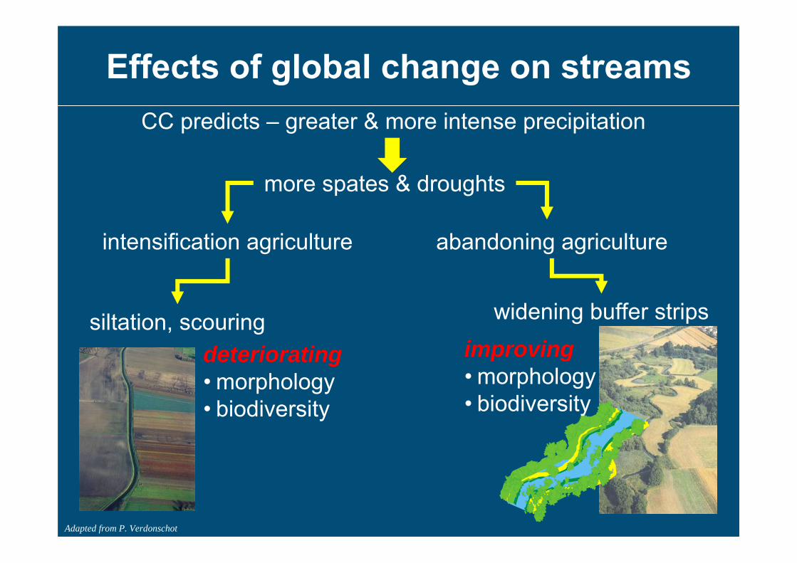
Effects of global change on streamsCC predicts – greater & more intense precipitation

more spates & droughts

abandoning agricultureintensification agriculture

siltation, scouringdeteriorating• morphology• biodiversity

widening buffer stripsimproving• morphology• biodiversity


Change , Yes we can: Climate ↔ hydrology ↔ species

(data CEH)

• Catchment model explained 69% of discharge variation• UK chalk geology: higher winter discharges

0

1

2

3

4

5

Jan Feb Mar Apr May Jun Jul Aug Sep Oct Nov Dec

Month

Dis

char

ge (c

umec

s) +

inte

rqua

rtile

rang

e

1974-19952071-2100

10 km10 km10 km

river Lambourn catchment (235 km2)

Climate modelPRUDENCE B2 med-low (RCAO HadAM3H model)

Catchment rainfall-runoff modelIHACRES


Change , Yes we can: Land-use ↔ Habitat ↔ species

(data BOKU)

• Siltation at the disturbed site due to land-use change (drainage)• Most habitats present at disturbed site, though many < 5%

reference site disturbed site

homogeneoussubstratum

heterogeneoussubstratum


• Land-use and hydromorphology were good predictors of fish assemblages• Climate, land-use and local physical descriptors were species-specific

(data CNRS)

46 Fish taxa11 spp selected

Clustering by SOM (Self Organising Map)

Prediction by MLP-BP (Multi-Layer Perceptron with backpropagation algorithm)

picture by Gomez Caruana, F.

1

2

3

4

0

0.34

0.8Barbatula barbatula

0

0.34

0.8Barbatula barbatula

0

0.44

0.94Phoxinus phoxinus

0.03

0.51

0.99Salmo trutta fario

0.03

0.51

0.99Salmo trutta fario

0.07

0.4

0.73Cottus gobio0.01

0.23

0.45Cottus poecilopus

0

0.34

0.88Leuciscus cephalus

0.01

0.4

0.8Rutilus rutilus0

0.37

0.82Gobio gobio

0

0.36

0.73Perca fluviatilis

0.28

0.56Esox lucius

0

0

0.28

0.56Leuciscus pyrenaicus

picture by De Falco, M.

98%

88%

97%

99% 93% 97%

99%

97%96%

98%100%

Land-use and hydromorphology -predictors of fish assemblages


STAR - streams types across Europe

STAR stream types

Lowlandstreams

Main stress gradients

Eutrophication / organic pollution

Hydromorphology

Land use

Sampling

Standardized sampling:

– Fish (electrofishing, 2 runs, 10 x width)

– Inverts (multihabitat, n = 20, composite)

– Macrophytes (100-m stream stretch)

– Diatoms (5 cobbles)

Environmental gradients -lowland streams

48% of variance explained by PC1 and PC2.

1st PC: % forest (+); % pasture (-), nutrients (-).

2nd PC: CPOM (+); stream order (-), cobble (-).

Studied biological response to these two orthogonal gradients

nutrients

habitat

Analyses

• Regressed measures of diversity (5) and assemblage composition (2) to two gradients (n = 66 streams)

• Three metrics of response models:• Precision (coefficient of determination),

• Sensitivity (magnitude of change, slope),

• Error (RMSEP)

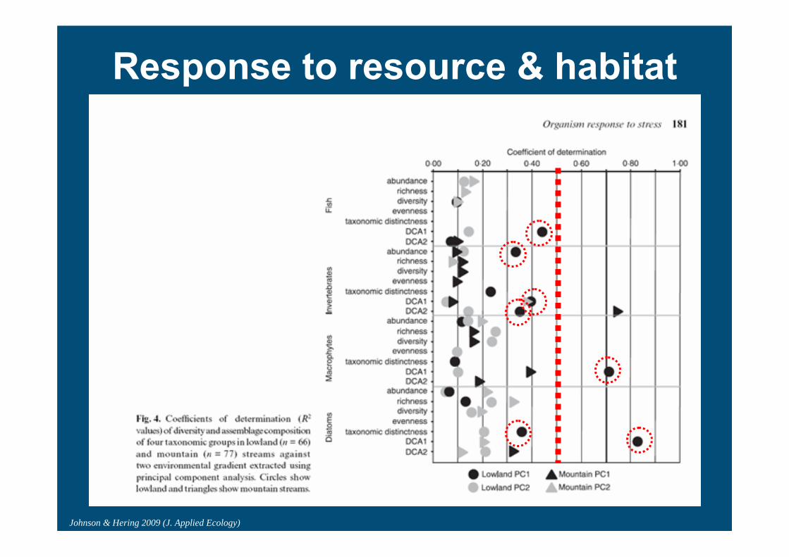
Response to resource & habitat

Johnson & Hering 2009 (J. Applied Ecology)

Assemblage response to resource gradient

Fish R2 = 0.44

Invertebrates R2 = 0.37

Macrophytes R2 = 0.70

Diatoms R2 = 0.82


• Responses were species-specific• Diatom assemblages collapsed at ca 50 µg P/L, invertebrates much higher

Assemblage response to habitat gradient

Fish R2 = 0.12

Invertebrates R2 = 0.05

Macrophytes R2 = 0.07

Diatoms R2 = 0.08


• All groups showed very weak responses to habitat gradient

PCA used to isolate

high & lowresource

&habitat groups

Johnson unpubl.

Not giving up; another approach

• All four groups showed clear differences between H and L resource groups

• ANOSIM – R values between 0.36 (macrophytes) and 0.81 (invertebrates)

Fish Invertebrates

Macrophytes Diatoms

Johnson unpubl.

Response to Resource(blue = H, red = L)

Response to Habitat(blue = H, red = L)

• All four groups showed considerable overlap between H and L habitat quality

• ANOSIM – only fish and invertebrates differed, but R values were low (< 0.20)

Fish Invertebrates

Macrophytes Diatoms

Johnson unpubl.

• Local factors more important than regional

• Response to resource gradient: diatoms ≥macrophytes > fish ≈ invertebrates

• Response to habitat gradient: macrophytes ≈diatoms > fish ≈ invertebrates

• Response trajectories differed between taxonomic group and stressor (nutrients –moderate to strong; hydromorphology – weak)BUT...multiple stressors at work?

Summary - scale, resource & habitat

Simple outcome: additive or multiplicative effect of all stressors combined equal to sum or productof individual effects.

Complex outcome: synergistic or antagonisticcombined effect larger or smaller than predicted from single effects.

Multiple stressors the norm not the exception!

Adapted from Townsend et al. 2008 (J. Applied Ecology )

Understanding effects of multiple stressors

Field survey - realistic but lacks control

Channel experiment - controlled but realism in question (i.e. appropriate temporal and spatial scale)

Reach-scale experiment - reasonably controlled and reasonably realistic


The survey

• 32 grassland streams in summer • 2nd order, homogeneous land-use (e.g. tussock

grass (least impaired) or pasture with sheep [impaired])– % sediment cover (S) – Log10DIN+Log10SRP (N)

• All variables normalized and scaled 0-1

• Multivariate models to quantify individual stressor effects and interaction Y=b1S + b2N + b3SN + bo


The reach-scale experiment

Nine relatively unimpacted streams (50 m reaches, 5 week experiment)

Complete factorial design -ambient, intermediate and high levels of both nutrients and sediment

Repeated measures ANOVA


The channel experimentEighteen channels (18 d experiment)

Complete factorial design -nutrients and sediment, also normal and 85% reduced dischargeANOVA: important terms are sediment and nutrients and the interactions:

Sediment * Nutrients

Sediment * Discharge

Nutrients * DischargeAdapted from Townsend et al. 2008 (J. Applied Ecology )

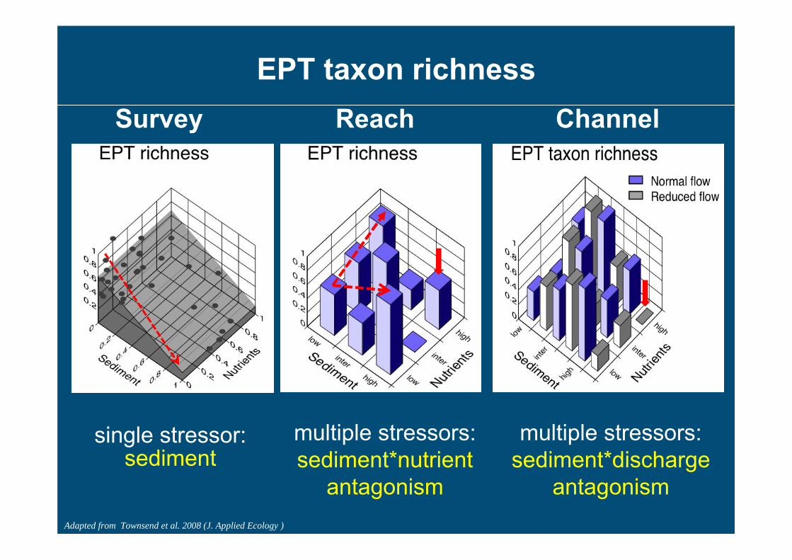
EPT taxon richnessSurvey Reach Channel

single stressor: sediment

multiple stressors: sediment*nutrient

antagonism

multiple stressors: sediment*discharge

antagonismAdapted from Townsend et al. 2008 (J. Applied Ecology )

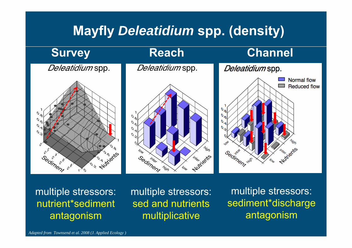
Mayfly Deleatidium spp. (density)Survey Reach Channel

multiple stressors: nutrient*sediment

antagonism

multiple stressors: sed and nutrients

multiplicative

multiple stressors: sediment*discharge

antagonismAdapted from Townsend et al. 2008 (J. Applied Ecology )

Relative importance of nutrients, sediment and discharge?

Nutrient effects

Sediment effects

Discharge effects

Survey 4 6Reach experiment 5 8Channel experiment 8 13 16


Summary - multiple stressorsSediment often more influential than nutrients

Abstraction perhaps more important than both

Surveys and experiments both offer something (not always the same result)

Survey - responses confounded by uncontrolled influences?

Experiments - scale appropriate?

Survey and, especially, experiments revealed many complex interactions

Managers may get it wrong if multiple stressors act in complex ways


Focus on nutrients vs hydromorphology

Timespan=1980-2009. Databases=SCI-EXPANDED.stream* and nutrient* = 3839stream* and hydromorpho* = 68

Since acceptance of WFDTimespan=2000-2009. Databases=SCI-EXPANDED.stream* & nutrient* = 2661stream* & hydromorpho* = 61

Web of Science®1980-2009 (22/2)

Is there a problem?

Is the problem easy to measure?

Do we know what to measure?

Hydromorphology alterations of streams

Yes

Not really

Nope

• How do we best establish the reference condition of streams where present-day analogues are lacking or too few (e.g. lowland streams)?

• Without drastically altering the landscape, is it possible to reconstruct the natural or near natural hydro-geo-morphology and structure and function of streams? How important is spatial configuration in stream restoration, e.g. for hydrology, for dispersal and colonization, etc?

• How important are terra-aquatic linkages for stream structure and function? Can use of large woody debris in stream restoration replace the function of mature riparian habitats?

• Many streams are affected by multiple stressors. Is it possible to separate the effects of multiples stressors on stream systems to best design and recommend management programs?

Some questions

“Landscape where the richness element is a little sunshine

innocent..”

Thoreau “Walden or life in the woods”

response of taxonomic groups in streams to gradients in...

Documents