response uncertainty and time-variant reliability...

*Correspondence to: Y. G. Zhao, Department of Architecture, Nagoya Institute of Technology, Gokiso, Showa-ku,Nagoya 466-8555, Japan.

Received 4 September 1998CCC 0098}8847/99/101187}27$17)50 Revised 2 February 1999Copyright ! 1999 John Wiley & Sons, Ltd. Accepted 4 May 1999

EARTHQUAKE ENGINEERING AND STRUCTURAL DYNAMICS

Earthquake Engng. Struct. Dyn. 28, 1187}1213 (1999)

RESPONSE UNCERTAINTY AND TIME-VARIANTRELIABILITY ANALYSIS FOR HYSTERETIC MDF

STRUCTURES

Y. G. ZHAO*, T. ONO AND H. IDOTA

Department of Architecture, Nagoya Institute of Technology, Gokiso, Showa-ku, Nagoya 466-8555, Japan

SUMMARY

Response uncertainty evaluation and dynamic reliability analysis corresponding to classical stochasticdynamic analysis are usually restricted to the uncertainties of the excitation. The inclusion of the parameteruncertainties contained in structural properties and excitation characteristics has become an increasinglyimportant problem in many areas of dynamics. In the present paper, a point estimate procedure is proposedfor the evaluation of stochastic response uncertainty, and a response surface approach procedure instandard normal space is proposed for analysis of time-variant reliability analysis for hysteretic MDFstructures having parameter uncertainties. Using the proposed procedures, the response uncertainties andtime-variant reliability can be easily obtained by several repetitions of stochastic response analysis undergiven parameters without conducting sensitivity analysis, which is considered to be one of the primarydi$culties associated with conventional methods. In the time-variant reliability analysis, the failure prob-ability can be readily obtained by improving the accuracy of the "rst-order reliability method using theempirical second-order reliability index. The random variables are divided into two groups, those with CDFand those without CDF. The latter are included via the high-order moment standardization technique.A numerical example of a 15F hysteretic MDF structure that takes into account uncertainties of fourstructural parameters and three excitation characteristics is performed, based on which the proposedprocedures are investigated and the e!ects of parameter uncertainties are discussed. Copyright ! 1999John Wiley & Sons, Ltd.

KEY WORDS: parameter uncertainty; response uncertainty; time-variant reliability; hysteretic MDF struc-ture; point-estimates; response surface approach

1. INTRODUCTION

The response uncertainty evaluation and dynamic reliability analysis corresponding to theclassical stochastic dynamic analysis are usually restricted to the uncertainties of the excitation.However, it has recently been recognized that the model parameters such as geometry materialproperties and excitation characteristics, are often poorly understood and the inclusion of theseparameter uncertainties has become an increasingly important problem in many areas of

dynamics.!"# The present paper attempts to evaluate the response uncertainty and dynamicreliability of hysteretic MDF structures a!ected by the parameter uncertainties included in thestructural properties and excitation characteristics.

For response uncertainty evaluation, early research monographs in this "eld, addressing bothstatic and dynamic problems, include the structural parameters by adopting series expansions inorder to evaluate the structural response.!$% In the framework of dynamic stochastic response,studies of uncertain linear systems with deterministic loads may be classi"ed into statisticalfrequency-domain analysis& and time-domain analysis.' The conventional approach in thedynamic analysis of structural systems with stochastic uncertainties is based on the seriesexpansion of stochastic quantities with respect to stochastic uncertainties and evaluates the"rst- and second-order moments of the response by solving deterministic equations once theperturbation method is applied. Some recent studies($) have shown that assuming the "rst-orderapproximation of the mean response to be coincident with the deterministic solutions, obtainedby "xing the stochastic mean value, can cause signi"cant error when the coe$cients of variationof stochastic parameters are relatively large. Therefore, in order to solve static problems, animproved approach that takes into account the "rst- and second-order probabilistic informationof stochastic parameters for computing the mean solution has been proposed. In the improvedapproach, the variance and covariance of the solutions are calculated using the improved meansolution rather than the mean solution.

Another improved approach!* has been proposed for evaluating in the time domain thestatistical moments of the response of linear systems subject to time-variant deterministic input.This method requires (1) a second-order Taylor series expansion with respect to the uncertainparameters, (2) introduction of the state vector space in order to obtain the "rst-order di!erentialequations and (3) adoption of the improved statistical moment into the "rst-order deterministicdi!erential equations.

All of these methods, which are referred to here as series expansion methods, have the followingweaknesses:

(1) The sensitivity of the response is required. Obtaining the sensitivity of the response,however, is not always easy because the response analysis includes complicated proceduressuch as eigenvalue analysis and the solution of line equations.

(2) Application to non-linear systems is di$cult. This is partially due to the fact that thesensitivity analysis in a non-linear system is much more di$cult than that in a linear system.

(3) Only the case of deterministic input, or the parameter uncertainties contained in structuralproperties are considered. In reality however, evaluation of response uncertainty due toboth the excitation characteristics and the structural properties under random processinput is also required, which is complicated if done using series expansion methods.

In order to evaluate the uncertainties of stochastic response due to parameter uncertainties, thepresent paper proposes a point estimation procedure, in which the stochastic response, includingparameter uncertainties, is obtained by several repetitions of stochastic response analysis undergiven parameters. In the case of non-linear dynamic analysis under stochastic excitation, theproposed procedure can be easily performed, without conducting any sensitivity analysis, whichis considered to be one of the primary di$culties associated with conventional methods.

On the other hand, for time-variant reliability analysis, to include parameter uncertainties, onecan "rst solve the problem with given parameters and then integrate over the system parametersto "nd the overall reliability. However, the computation could become excessive since repeated

1188 Y. G. ZHAO, T. ONO AND H. IDOTA

Copyright ! 1999 John Wiley & Sons, Ltd. Earthquake Engng. Struct. Dyn. 28, 1187}1213 (1999)

solutions of stochastic structural response are required, and so an approximate method havinggood accuracy and numerical e$ciency is needed. For a linear oscillator, a First-Order Reli-ability Method (FORM) was proposed by Hohenbichler and Rackwitz in which the distributionof the maximum peak of the response is used.!! This method has been used in the case ofnon-stationary excitation by Balendra and Quek.!%$!+ For general problems, reliabilityestimation methods have been proposed by Gueri and Rackwitz,!, for which auxiliary variablesare introduced so that FORM can be used. A more general discussion of time-variant structuralreliability analysis is provided by Wen and Chen,, where only one auxiliary random variableis introduced and a performance function was proposed. This method has been applied tosystem reliability by Wen and Chen.!#$!& Incorporating these methods, a nested FORM hasbeen proposed by Madsen and Tvedt!' based on the discussion of the calculation of the failureprobability with given parameters. In these methods, which enable an evaluation of thedynamic structural reliability that includes parameter uncertainties to be performedusing FORM, calculating the gradients of the performance function is an important step.Because it is not always easy to obtain these gradients,!( a spectral stochastic "niteelement formulation using polynomial chaoses has been proposed%$+ and the Response Sur-face Approach (RSA) has recently been introduced!) to avoid the di$culties in obtainingthe gradients.

Because time-variant reliability in the above methods is conducted using FORM, the problemof accuracy will arise for the case of a strong non-linear performance function. To improve theanalytical accuracy, the Second-Order Reliability Method (SORM) may be used, but the compu-tation of Hessian matrix and its the rotational transformation are necessary.%*$%! On the otherhand, in all the above methods, the random variables that express the parameter uncertainties aregenerally expressed as continuous random variables that have a known Cumulative DistributionFunction (CDF). In reality however, due to the lack of statistical data, the CDF of some randomvariables may be unknown, and their probabilistic characteristics may be expressed using onlystatistical moments.

In order to improve the two weaknesses described above, a computational procedure of RSAin standard normal space is proposed. In this procedure, the time-variant reliability analysisis conducted through several repetitions of dynamic reliability analysis with given parameters,and without any sensitivity analysis. Because the response surface is directly obtainedas a polynomial of standard normal random variables, neither a complicated computation ofthe Hessian matrix is needed, nor is it necessary to carry out its rotational transformationand eigenvalue analysis. In order to include the random variables having no CDF, therandom variables included in the analysis model are divided into two groups, thosehaving continuous CDF, such as sti!ness, damping, and strength, and those having no CDF,such as excitation characteristics. Random variables having no CDF are included via theHigh-Order Moment Standardization Technique (HOMST), the use of which requires almostno extra e!ort.

2. NON-LINEAR STOCHASTIC RESPONSE AND RELIABILITY ANALYSISWITH DETERMINISTIC PARAMETERS

The uncertainties in classical stochastic dynamic analysis are usually restricted to excitation. Forhysteretic MDF structures, the non-linear random vibration analysis is generally conducted

RESPONSE UNCERTAINTY AND TIME-VARIANT ANALYSIS OF MDF STRUCTURES 1189


using equivalent linearization,%%$%+ and the equivalent sti!ness and equivalent damping ratio aredetermined according to random vibration theory using the following equations%,

K!(!)"K

*!

[(1!")(1#ln !)#"!] (1)

#!(!)"#

*#0)15 !1!1

!!1#" (!!1)" (2)

where K!

is the equivalent sti!ness, #!

is the equivalent damping ratio for the nth mode," is the sti!ness ratio, ! is the ductility ratio, K

*is the initial sti!ness and #

*the damping

ratio.Assume the ground acceleration is idealized as a segment of "nite duration of a stationary

Gaussian process having mean of zero. Using the random mode decomposition method com-bined with the mean-value response spectrum,%#"%' the deviation of the stochastic response isobtained as

$%""!

"

!#

B"B

#%*$"#

!&*$""

&*$##

(3)

where B"is the participation factor of the ith mode obtained by dynamic analysis of structures,

%*$ "#

is the correlation coe$cient between the ith and jth modes, which can be obtained fromrandom vibration analysis, and &

*$""is the spectral moment of ith mode, which can be obtained

from the mean-value response spectrum.Using the result of the standard deviation of response $

"obtained from random vibration

analysis, the mean value and standard deviation of the maximum response are obtained using thefollowing equations:

'#"$

" !!2 ln (D# 0)5772

!2 ln (D" (4)

$#" )$

"!12 ln (D

(5)

where '#

and $#

are the mean value and standard deviation, respectively, of the maximumresponse, ( is the mean cross ratio, and D is the duration of ground motion.

After obtaining the deviation of the stochastic response, failure probability is de"ned as the "rstpassage probability of the maximum response, the probability distribution of which is assumed tobe given by

F"(u)"exp #!(D exp !!1

2 $ u$"%%"& (6)

where ( is the cross ratio, and $"is the standard deviation of the stochastic response obtained

from stochastic vibration analysis.



3. STOCHASTIC RESPONSE INCLUDING PARAMETER UNCERTAINTIES

3.1. Stochastic response with parameter uncertainties

In the analysis described in the previous section, all input parameters, including structuralproperties and excitation characteristics, are assumed to be deterministic. When these parameteruncertainties are included in the analysis, the parameters are expressed as random variablesX and the maximum response can be expressed as a function of X

R#$%

"R#(X) (7)

In evaluating the response uncertainty due to the parameter uncertainties, the method gener-ally employed is to expand R

#$%to a Taylor series and conduct the evaluation using a "rst-order

approximation!$%( as shown below:

$%-

"!$

!#

*R#

(X)*x

$

*R#

(X)*x

#

%$#

$$$#

(8)

where $$is the standard deviation of x

$and %

"#is the correlation coe$cient of x

$and x

#.

No explicit description of R#$%

is given in random vibration theory (only its mean value '#

andstandard deviation $

#, expressed by equations (4) and (5), are given). The gradients of R

#$%are

di$cult to obtain because the random vibration analysis is non-linear and the gradient analysisprocedure includes several complicated procedures, such as the inverse distribution function,eigenvalue analysis, the computation of the participation factor and the spectral moments.!( Inorder to avoid the di$culties associated with the computation of gradients, the present paper willevaluate the mean value '

-and standard deviation $

-of R

#$%utilizing the computational results

of equations (4) and (5).After including the parameter uncertainties described by random variables X, the mean value

'#

and standard deviation $#, expressed in equations (4) and (5) become functions of X, denoted

by '#(X) and $

#(X), respectively. For a group of given values of X, the values of the functions

'#(X) and $

#(X) can be obtained using the method described in the previous section. To include

the uncertain parameters X, functions '#(X) and $

#(X) can be computed for given X, after which

these functions can be integrated over the entire area for which X is de"ned to obtain the meanvalue '

-and standard deviation $

-of the maximum response.

Since

'#(X)"' R

#(X) f (R

#+X) dR

#(9)

$%#(X)"' (R

#(X)!'

#(X))% f (R

#+X) dR

#(10)

'-

and $-

can be expressed as the following equations:

'-"' R

#(X) f (R

#+ X) f (X) dR

#dX"E['

#(X)] (11)

$%-"' (R

#(X)!'

-)% f (R

#+X) f (X) dR

#dX"E[$%

#(X)]#E['%

#(X)]!'%

-(12)



where

E[ ) (X)]"'%

) (X) f (X) dX (13)

The distribution f (R#

+ X) is presented only in order to facilitate description, and is not requiredfor the evaluation.

In order to evaluate E['#(X)], E['%

#(X)], and E[$%

#(X)], Monte-Carlo simulation or direct

integration may be used. A large number of repetitions of non-linear stochastic analysis isrequired. Another general approximation is obtained from the Taylor expansion of thesefunctions,%( in which the previously described di$culties in the computation of derivativesdescribed above will be encountered. The response surface approach can be used to avoid thedi$culties in computation of derivatives. However, according to our computational experience,the results of this approximation depend strongly on the "tting points. Therefore, an approxima-tion method that is both e$cient and accurate is required. The present paper evaluates E['

#(X)],

E['%#(X)], and E[$%

#(X)] using the method of point estimates.

3.2. Concept of point estimates

The method of point estimates was proposed by Rosenblueth%) for estimating the "rst fewmoments of a function of random variables. This method uses a weighted sum of the functionevaluated at a "nite number of points. The weights and points at which the function is evaluatedare chosen as the weights and points at which the variable itself must be evaluated to give thecorrect "rst few moments of the variable itself, i.e. the estimating points x

!, x

%,2,x

&and the

corresponding weights p!, p

%,2, p

&are selected using the following equations:

&!".!

p""1 (14)

&!".!

p"x""'

%(15)

&!".!

p"(x

"!'

%)!"' (x!'

%)! f (x) dx (16)

where f (x) is the PDF of x, and '%

is the mean value of x.For a three-point estimate, let the concentrations be p

", and x

", p

*and x

*, and p

'and x

'.

Gorman+* derived the following equations for x"

, x*, x

'and p

", p

*, p

':

p"

"12 $1#"

+%/,

",%

!"%+%% (17)

p*"1! 1

",%

!"%+%

(18)

p'

"12 $1!"

+%/,

",%

!"%+%% (19)

x"

"'%!$

%2

(,!"+%

) (20)



x*"'

%(21)

x'

"'%#$

%2

(,#"+%

) (22)

where,"(4"

,%!3"%

+%)!/% (23)

For a function of y"y (x), the kth central moment of y can be calculated using x"

, x*, x

', p

",

p*, and p

'

$$("$(

"p"

(y"

!'()$#p

*(y

*!'

()$#p

'(y

'!'

()$ (24)

where the mean value and standard deviation of y"y (x) are as follows:

'("p

"y"

#p*y*#p

'y'

(25)

$%("p

"[y

"!'

(]%#p

*[y

*!'

(]%#p

'[y

'!'

(]% (26)

3.3. Point estimates for a function of n variables

The procedure leading to equations (17)}(26) has been generalized to a function of multiplevariables Z"G(X), where X"x

!, x

%,2,x

!. The joint probability density is assumed to be

concentrated at points in the 2! hyperquadrants of the space de"ned by X. For a large n, thenumber of function recalls of G (X) will be too large for practical applications. Rosenblueth%)approximated G(X) using the following function:

Z"G-(X)"G*!.".!$Z

"G*% (27)

and Idota et al.+! approximated G(X) using the following function:

Z"G-(X)" !!".!

(Z"!G*)#G* (28)

whereZ

""G('

!,2, '

""!, x

", '

"'!,2, '

!) (29)

G*"G('!,2,'

",2, '

!) (30)

The mean value and standard deviation of approximation (27) are expressed as

')"G*

!.".!$')"G*% (31)

$%)".!

".!($%

)"#'%

)")

(G*)%0!"!1!'%

)(32)

The mean value and standard deviation of approximation (28) are expressed as

')" !

!".!

(')"

!G*)#G* (33)

$%)" !

!".!

$%)"

(34)



where ')"

, and $)"

are the mean value and standard deviation, respectively, of Z"which are

obtained using equations (25) and (26).Using equations (27)}(34), only 2n#1 function calls of G(X) are needed for computation of

mean value and standard deviation of G(X) having n random variables.Substituting the functions '

#(X), '%

#(X) and $%

#(X) in the previous section for G(X) in equation

(27) or equation (28), point estimates for E['#(X)], E['%

#(X)] and E[$%

#(X)] can be obtained, and

the mean value '-

and deviation $-

of the maximum response can be evaluated.

3.4. Investigation on the method of point estimates

In the "rst example, consider the following function of a standard normal random variable:

y"exp(u/#&) (35)

where & and / are parameters. In the present example, &"1)5 and /"0)1}0)6 are assumed.The variable y is a lognormal variable with parameter & and /, and the "rst four moments are

expressed exactly as

'("exp (&#!

%/%) (36a)

$%("'%

((0!1) (36b)

"+"!0!1 (0#2) (36c)

","0,#20+#30%!3 (36d)

where

0"exp(/%), (36e)

"+

and ",

are the third and fourth order dimensionless central moments, i.e. skewness andkurtosis of y, respectively.

The "rst four moments obtained using equations (24), (25) and (26) are depicted as (a), (b), (c)and (d) in Figure 1 along with the corresponding theoretical values. Figure 1 reveals that themean value and standard deviation obtained by point estimates are in very good agreement withthe exact values, but for third- and fourth-order moments, the results obtained by point estimatescannot be used as an approximation of the exact values.

In the second example, consider the following function of a lognormal normal randomvariable:

y"ln(x) (37)

where x is a lognormal variable with parameters & and #. In the present example, &"1)5 and/"0)1}0)5 are assumed.

The variable y is a normal random variable and the "rst four moments can be readily obtainedas '"&, $"/, "

+"0, "

,"3, exactly.

The "rst four moments obtained using equations (24), (25) and (26) are depicted as (a), (b), (c),and (d) in Figure 2 along with the corresponding theoretical values. Figure 2 shows that the ' and$ obtained using point estimates are in very good agreement with the exact values when / isassumed to be small (below 0)4). The accuracy of the results obtained using point estimatesdecreases as the order of the moments to be evaluated increases. For "

+and "

,, the results

obtained using point estimates cannot be used as an approximation of the exact values. Also note



Figure 1. Point estimates for Example 1

that if the deviation of the random variable x is large, the estimating point x obtained usingequation (20) becomes negative, and is therefore out of the de"nition area of the variable.

These two examples show that point estimates are only applicable for lower-order moments offunctions of random variables with small deviation. Since the evaluation of response uncertaintydescribed in Section 3.1 includes only the mean value of the functions '

#(X), '%

#(X) and $%

#(X),

point estimates are applicable in the present study.

4. TIME-VARIANT RELIABILITY ANALYSIS METHOD

4.1. Extensive xrst-order reliability method

In order to include the parameter uncertainties, one can "rst solve the problem with givenparameters and then integrate over the system parameters to "nd the overall reliability, providedthe probability information for the parameters is available. The integral is shown as

P2"'X

P&(X) f (X) dX (38)



Figure 2. Point estimates for Example 2

where P&(X) is the conditional failure probability for a given X, which is evaluated using

state-of-the-art techniques, and f (X) is the joint probability density function of X.However, the computation could become excessive since repeated solutions of stochastic

structural response are required, and so an approximate method having good accuracy andnumerical e$ciency is needed. Therefore, Wen and Chen, developed the following performancefunction in standard normal space, in which only one auxiliary random variable is introduced.

G(X, u!'!

)"u!'!

!1"![P&(X)] (39)

The gradients of the performance function with respect to U are given by

#*G*u

"&")!

"![J"!!

]3 #*[P&(X)

*x"&")!

(40)

where U is the standard normal variable vector transformed from X by Rosenblatt transforma-tion, and u

!'!is a standard normal random variable independent of U. [J] is the Jacobian matrix

for the transformation of variables.



This performance function enables an evaluation of the dynamic structural reliability thatincludes parameter uncertainties to be performed using FORM and is referred to as ExtensiveFORM (EFORM) in the present paper. Calculation of the gradients of the performance functionis an important step of the EFORM. However, it is not always easy to obtain these gradients,!(especially for the case where non-linearity of the structural performance is considered. In orderto avoid such di$culties in obtaining the gradients, in this paper the performance function isapproximated using Response Surface Approach (RSA).!)

4.2. Response surface approach in standard space

RSA is a statistical analysis method that examines the relationship between experimentalresponse and variations in the values of input variables. The basic concept of RSA is to replace theoriginal implicit performance function by an approximated explicit function (generally a second-order polynomial) expressed in terms of basic random variables.+%"+, For time-variant reliabilityanalysis, Yao and Wen!) have introduced RSA to avoid the sensitivity analysis required inEFORM. However, because the response surface function is expressed as a polynomial of basicrandom variables in original space, when the computational accuracy of failure probabilityis improved by using SORM, it is necessary to compute the Hessian matrix, and to carry outits rotational transformation and eigenvalue analysis. Alternatively, one can use the point-"ttingSORM approximation+# after the response surface has been obtained, but additional iteratione!ort will be needed.+& In order to improve on this weakness, in this paper the performancefunction is directly approximated in standard normal space. This has the following twoadvantages:

(1) Because the response surface function is expressed directly as a second-order polynomial ofstandard normal random variables, it is very simple to obtain the second-order derivativematrix (the scaled Hessian matrix) and compute the failure probability using the simpleapproximation of SORM.+#$+'

(2) In RSA, "tting points are controlled by their distance from the original point, which isgenerally expressed as a multiple of the standard deviation of the random variable. If theresponse surface function is expressed as the function of standard normal random vari-ables, the factors become very simple. This is because all the standard deviations of all thestandard normal random variables are equal to 1.

For simpli"cation, the performance function shown in equation (39) is approximated by thefollowing second-order polynomial of standard normal random variables, in which the mixedterms are neglected

G-(U)"a*#u

!'!# !

!#.!

!#u## !

!#.!

&#u%#

(41)

where a*, !

#, and &

#are 2n#1 regression coe$cients with j ranging from 1 to n.

If the practical performance function G(U) in equation (39) is "tted by G-(U) of equation (41) atthe "tting points in the vicinity of the design point, the regression coe$cients a

*, !

#, and &

#can be

determined from the linear equations of a*, !

#, and &

#obtained at each "tting point.

For the obtained design point U'in standard normal space, "tting points along the co-ordinate

axes are selected. Along each axis u#, j"1,2, n, two points having the co-ordinates (U-

', u

'#!2)



and (U-', u

'##2) are selected, where U-

'"3u

'$, k"1,2, n except j4 represents the co-ordinates

of the design point along all the axes except the j-axis, and 2 is a factor which represents thedistance from the central point to the "tting point. Transform the "tting points into original spaceusing Rosenblatt transformation, and "t the original performance function by the performancefunction approximation in equation (41) at these points. The regression coe$cients in equation(41) can now be obtained.

Because the design point is not generally known beforehand, this paper uses the iterative RSAprocedure in the point-"tting SORM+# to approach the performance function in the course ofobtaining the design point. Using the procedure, only m(2n#1) repetitions of nonlinear randomvibration analysis are required for evaluation of time variant reliability with n random variables,where m is the number of iterations. As shown in the ensuing sections of the present paper, thisprocedure is reasonably accurate.

4.3. Computation of failure probability

After obtaining the response surface function shown in equation (41), the "rst-order reliabilityindex and its corresponding failure probability can be readily obtained. For the case of a strongnon-linear performance function, in order to improve the analytical accuracy, the failure prob-ability can be obtained using MCS or SORM. In this paper, the failure probability is computedusing the empirical SORM reliability index.+'

Because the response surface function has the same form as the point-"tted performancefunction,+# the scale Hessian matrix corresponding to equation (41) is readily obtained as

B" 2+5G- +

&!

2 0

6 ! 60 2 &

!

(42)

where

+5G- +"(1# !!#.!

(!##2&

#u*#) (43)

The sum of the principle curvatures and the average principle curvature radius of the limit statesurface at design point U* can be expressed as:+#

K4" 2

+5G- +!!#.!

&# !1! 1

+5G- +%(!

##2&

#u*#)%" (44)

R"n!1K

(

(45)

With the aid of K(

and R expressed in equations (44) and (45), the failure probabilitycorresponding to the point-"tted performance function (response surface function) can beobtained by substituting equations (44) and (45) in the following empirical second-order reliabil-ity index, which is in closed form:

7("!1"! !1(!7

2) $1# ! (7

2)

R1(!72)%"0!"!1/%0!'%*(/!*0!'%"211" , K

(*0 (46)



7("$1# 2)5K

(2n!5R#25(23!57

2)/R%% 7

2#1

2K

( $1#K(

40% , K((0 (47)

where K(is the sum of the principle curvatures of the limit state surface given as in equation (44),

R the average principle curvature radius given as in equation (45), n the number of randomvariables, 7

2the "rst-order reliability index and 7

(the second-order reliability index.

4.4. Inclusion of random variables having no CDF

In the analysis method described above, all random variables are assumed to be continuousvariables having a known CDF. However, the CDF of some of these variables may not beactually obtainable, and their probability information may be expressed only as cumulatemoments. In order to include these random variables, the High-Order Moment StandardizationTechnique (HOMST)+($+) is used.

When the CDF of a random variable cannot be obtained, the histogram is assumed to beobtainable from statistical data. The failure probability of equation (38) can be expressed in sumform:

P2"!

"

P&(x

")h(x

")8x

"(48)

where P&(x

") is the conditional failure probability when the random variable takes the given value

of x"x", and h(x

") is the value of the histogram when x is equal to x

".

Using HOMST, the random variable can be transformed into a standard normal randomvariable by the high-order moment standardization function S,

y"x!'%

$%

(49)

u"1a

["+(

#3(",(

!1)y!"+(

y%] (50)

a"!(5"%+(

!9",(

#9) (1!",(

) (51)

where "$(

is the kth-order dimensionless central moment of y, which is equal to the kth-orderdimensionless central moment of x according to the de"nition of high-order moment, u is thestandard normal random variable.

Because u is a continuous random variable, a continuous random variable x- can be obtainedby the inverse transformation S"! corresponding to u.

x-"S"!(u) (52)

Although x and x- are di!erent random variables, they correspond to the same standardnormal random variable and have the same high-order moments and the same statisticalinformation source. Therefore, f (x-) can be considered to be an anticipated continuous distribu-tion of x. Using this continuous distribution, the failure probability shown in equation (48) canagain be expressed as in equation (38), and reliability analysis can be performed using theEFORM equations described in the previous section. The Jacobinan matrix can be obtaineddirectly from equations (49), (50) and (51), instead of from the Rosenblatt transformation:

J"""*u

"*x

"

" 1a$

%

[3($,(

!1)!2"+(

y] (53)



and the inverse function of S is expressed as

x-" $%

2"+

[3(",!1)!!9("

,!1)%#4"

+("

+!ua)]#'

%(54)

When both random variables having continuous CDF and those having no CDF are con-sidered, the random variables can be divided into two groups X"[X

!, X

%], where X

!are the

random variables having CDF, and X%

those having no CDF. For X%, using the anticipated

distribution f%(X-

%) obtained from HOMST described above for X

%, the total failure probability

can be written as

P2"'X

!$X5%

P&(X

!, X-

%) f

!(X

!) f

!(X-

%) dX

!dX-

%(55)

Equation (55) can be solved using the EFORM combined with the RSA in standard normalspace described in the previous section. When doing this, the Jacobian matrix of X

!is obtained by

Rosenblatt transformation, and that of X%

is obtained using HOMST. In this way, the randomvariables without CDF can be included with almost no extra e!ort. Note that the histogram h (x

")

and the anticipated distribution f%(X-

%) of X

%are not needed in the computation; they are used

here only for convenience of description.

5. NUMERICAL EXAMPLE AND INVESTIGATIONS

5.1. Structural model and conditional random vibration analysis

In this section, the response uncertainty and time-variant reliability analysis for a 15F steelstructure having a total height of 52)5 m is performed. The height, weight, initial sti!ness andstrength of each #oor are listed in Table I. The structural model is assumed to be a shearinghysteretic MDF model, and the force}deformation relationship is assumed to be bilinear. Thedamping and sti!ness ratios are assumed to be 0)02 and 0)05, respectively.

The acceleration spectrum recommended by the Architecture Institute of Japan (AIJ),* is usedas the earthquake input and is expressed as

S+(!, h)"# $

1#f+!1d % F

,G+R+A

*0)!)d!

'

F,G+R+A

*d!

')!)!

'2)F

,G-R

-<*

! !')!

(56)

where f+, f

-, d, G

+, G

-, and !

6are parameters of the response spectrum and are assumed to be

2)5, 2)5, 0)5, 1)2, 2)0, and 0)55, respectively, according to the recommendations of the AIJ.,*As the input of the peak ground acceleration, the maximum value of 818 gal, obtained on

January 17th, 1995 during the Hanshin-Awaji earthquake, is used. The computational resultsusing deterministic structural parameters are listed in Table II, in which R

#$%represents the

maximum response of relative storey displacement. Table II shows that all #oors enter the ductilearea when subjected to the previously mentioned input. The maximum ductility ratio occurs at



Table I. Structural parameters

Floor H (cm) = (t) K (t/cm) Q (t) K!/K

*

15 400 397 404 490 0)0514 400 1278 615 1909 0)0513 335 1909 1084 3044 0)0512 310 1400 1429 3739 0)0511 310 1386 1687 4216 0)0510 310 1465 1979 4464 0)059 310 1624 2200 5271 0)058 310 1595 2488 5665 0)057 310 1615 2889 6141 0)056 310 1961 3347 5669 0)055 450 3546 2999 5953 0)054 450 4613 2909 7224 0)053 500 5802 2803 8735 0)052 400 7593 3625 9922 0)051 475 6007 4507 10330 0)05

H: Floor height =: Floor weightK: Initial sti!ness Q: Initial strengthK

!/K

*: Sti!ness ratio

Table II. Stochastic response using deterministic parameters

Floor $"

' of R#$%

Duct. ratio $ of R#$%

P&

7

15F 0)877 2)30 1)90 0)46 0)0 #14F 2)293 6)16 1)98 1)21 0)0 #13F 2)892 7)62 2)71 1)57 0)0 #12F 2)880 7)47 2)85 1)59 0)0 #11F 2)988 7)52 3)01 1)68 1)2#10"' 5)6010F 3)100 7)68 3)40 1)77 1)0#10"# 4)279F 2)944 7)25 3)03 1)71 2)9#10"' 5)008F 2)894 7)09 3)11 1)69 9)5#10"' 4)767F 2)655 6)52 3)07 1)50 6)5#10"' 4)846F 2)917 7)16 4)23 1)72 2)0#10"+ 2)885F 3)947 9)60 4)84 2)34 1)7#10"% 2)124F 4)276 10)26 4)13 2)55 1)5#10"+ 2)973F 4)662 11)22 3)60 2)77 8)0#10"# 3)772F 4)168 10)16 3)71 2)44 1)3#10", 3)651F 3)599 8)97 3)91 2)05 3)2#10", 3)41

the "fth #oor, and the corresponding mean value of maximum response is found to be 9)60 witha standard deviation of 2)34.

Assuming the excursion level is taken to be 7 based on the deformation capacity of buildings inseismic design recommended by the AIJ,,! the computational results of failure probability withgiven parameters are listed in Table II. The conditional failure probability corresponding to the"fth #oor is found to be 0)017.



5.2. Parameter uncertainties

Seven parameters, four structural parameters and three excitation characteristics, have beenconsidered. The uncertainty of structural parameters, the initial sti!ness K

*, initial strength Q

*,

#oor weight = and damping ratio # in each #oor are assumed to be totally correlated. Eachparameter is multiplied by a random variable having a unit mean value

K-*"x

*K

*(57a)

Q-*"x

.Q

*(57b)

=-"x/= (57c)

#-"x$# (57d)

D-"x0D (57e)

S-+"x

1S+

(57f )

where x*, x

., x

/, x$ , x0

and x1

are random variables having a mean value of 1. K*, Q

*, =, #,

D and S+

are the deterministic values of initial sti!ness, yield strength, #oor weight, dampingratio, duration and response spectra, respectively, and K-

*, Q-

*, =-, #-, D- and S-

+are the

corresponding variables that include uncertainties.According to References 4, 28, 38 and 41, x

*, x

., x

/, x$ , x0 are assumed to be lognormal

random variables with coe$cients of variation of 0)1, 0)2, 0)1, 0)4 and 0)3 respectively. The "rstfour moments of the standard response spectrum are taken to be '"1)0. $"0)26, "

+"0)798,

","7)152 according to Reference 28.The distribution of the peak ground acceleration a

)is obtained directly from th excursion

probability curve of the annual peak ground acceleration under the assumption that theearthquake occurs in accordance with the Poisson's Law:

f+(a)"$ "

a*%$ a

a*%"0%'!1

(58)

where a*

is the minimum value of a), which is taken to be 20 gal, and " is taken to be 2)34.

5.3. Response uncertainty evaluation

In order to investigate the evaluation procedure for response uncertainty, the uncertainties ofonly four parameters, i.e. x

*, x

., x

/and x$ are considered. All four random variables have known

CDF, so the results can be con"rmed using the Monte-Carlo Simulation (MCS). Evaluations areconducted using the approximation functions given in equations (27) and (28). The standarddeviations of the maximum response obtained using point estimates are listed in Table III alongwith those obtained using MCS with a sample size of 10 000. Table III shows that although only2n#1"9 repetitions of nonlinear random vibration analysis are required in equations (27) and(28), both of these approximation functions yield good results. The largest error for equation (27)is 1)815 per cent and that for equation (28) is 2)383 per cent. That is to say, the results obtainedusing point estimates using either equation (27) or equation (28) can be used as an accurateapproximation of the actual values. Since the errors obtained using equation (27) are generallysmaller than those obtained using equation (28), the present paper will use equation (27) for the



Table III. Comparison of MCS and PEM with four parameter uncertainties (p ofmaximum response)

Floor MCS Point estimatesEquation (27) Error (%) Equation (28) Error (%)

1 2)3523 2)3096 1)815 2)2962 2)3832 2)7234 2)6936 1)094 2)6839 1)4513 3)0926 3)0475 1)458 3)0319 1)9644 2)8554 2)8083 1)649 2)7977 2)0205 2)6448 2)6237 0)798 2)6154 1)1136 1)8958 1)8829 0)680 1)8842 0)6107 1)6597 1)6535 0)373 1)6561 0)2158 1)7935 1)7935 0)000 1)7966 0)1739 1)8132 1)8235 0)568 1)8258 0)695

10 1)9009 1)9171 0)852 1)9194 0)97211 1)7939 1)8113 0)970 1)8150 1)17412 1)7015 1)7193 1)046 1)7229 1)25813 1)6691 1)6732 0)241 1)6689 0)01314 1)3607 1)3712 0)772 1)3765 1)16215 0)5303 0)5378 1)414 0)5390 1)646

evaluation of the uncertainties of the maximum response in which all the parameter uncertaintiesare considered.

In order to investigate the e!ect of the parameter uncertainties, the mean value of themaximum response using deterministic parameters, two parameter uncertainties (x

*and x

.only),

four parameter uncertainties (x*, x

., x

/and x$ only) and six parameter uncertainties

(x*, x

/, x$ , x0

and x1) are depicted in Figure 3, in which the inclusion of parameter uncertainties

is revealed to make the mean values of the maximum response larger for some #oors and smallerfor others. Generally, the inclusion of the parameter uncertainties have little e!ect on the meanvalue of the maximum response.

The standard deviation of the maximum response corresponding to Figure 3 are depicted inFigure 4, in which the deviations including parameter uncertainties are very di!erent from thoseusing deterministic parameters. From the comparison between Figures 3 and 4, one can see thatthe parameter uncertainties have a much greater e!ect on the standard deviation than on themean value of the maximum response. Figure 4 reveals that the greater the number of parameteruncertainties included, the larger the standard deviation of the maximum response. Since thestandard deviation using six parameter uncertainties is much larger than that using deterministicparameters, two parameter uncertainties and four parameter uncertainties, the e!ect of theuncertainties included in the excitation properties is found to be dominant on the uncertainties ofthe maximum response.

5.4. !ime-variant reliability analysis

In order to investigate the e$ciency of the procedure proposed for time-variant reliabilityanalysis, uncertainties of only two parameters, i.e. x

*and x

., are "rst considered. The "tting

points in standard normal space are controlled by 2"0)5.



Figure 3. Mean values of maximum response including parameter uncertainties

For the "fth #oor, convergence is reached easily after "ve iterations. The "rst-order reliabilityindex is obtained as 7

2"1)118, with corresponding failure probability of P

2"0)1319. Using the

SORM approximation described in Section 4)3, the sum of the principle curvatures of the limitstate surface is readily obtained as K

("0)0689, with a corresponding average principle curvature

radius of R"29)042. It can be seen from this that the non-linearity of the performance function isvery weak. With the aid of K

(and R, the second-order reliability index is obtained as 7

("1)151,

with corresponding failure probability of P("0)1249. For the purpose of comparison, MCS with

50 000 trials is also conducted and the failure probability is obtained as 0)1236. One can see thatthe SORM result obtained in this paper agrees with the MCS result quite well.

In order to investigate the procedure of the RSA, the response surface obtained after the "rst,third and "fth iterations are depicted in Figures 5}7, in which the black point is the design pointof the limit state surface and the dashed lines describe the coordinates of the design point. In these"gures, the surface with rough mesh is the response surface described by equation (41) and thatwith "ne mesh is the true limit state surface described by equation (39). From Figures 5}7, one cansee that although the response surface obtained after the "rst iteration does not approximate thetrue limit surface in the vicinity of the design point, as the number of iterations increases, theapproximation gradually becomes better. The response surfaces obtained after the "fth iterationagrees with the limit state surface quite well in the vicinity of the design point.



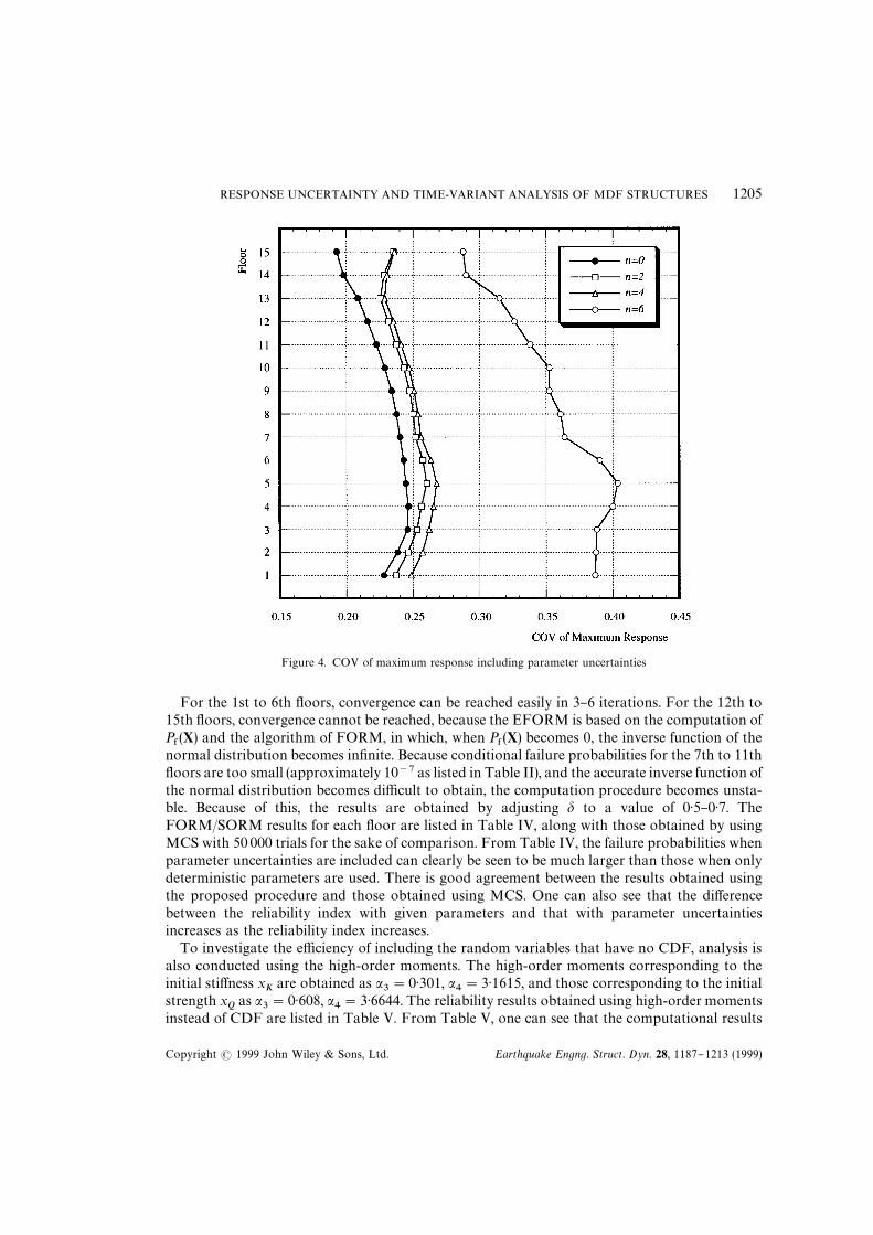
Figure 4. COV of maximum response including parameter uncertainties

For the 1st to 6th #oors, convergence can be reached easily in 3}6 iterations. For the 12th to15th #oors, convergence cannot be reached, because the EFORM is based on the computation ofP&(X) and the algorithm of FORM, in which, when P

&(X) becomes 0, the inverse function of the

normal distribution becomes in"nite. Because conditional failure probabilities for the 7th to 11th#oors are too small (approximately 10"' as listed in Table II), and the accurate inverse function ofthe normal distribution becomes di$cult to obtain, the computation procedure becomes unsta-ble. Because of this, the results are obtained by adjusting 2 to a value of 0)5}0)7. TheFORM/SORM results for each #oor are listed in Table IV, along with those obtained by usingMCS with 50 000 trials for the sake of comparison. From Table IV, the failure probabilities whenparameter uncertainties are included can clearly be seen to be much larger than those when onlydeterministic parameters are used. There is good agreement between the results obtained usingthe proposed procedure and those obtained using MCS. One can also see that the di!erencebetween the reliability index with given parameters and that with parameter uncertaintiesincreases as the reliability index increases.

To investigate the e$ciency of including the random variables that have no CDF, analysis isalso conducted using the high-order moments. The high-order moments corresponding to theinitial sti!ness x

*are obtained as "

+"0)301, "

,"3)1615, and those corresponding to the initial

strength x.

as "+"0)608, "

,"3)6644. The reliability results obtained using high-order moments

instead of CDF are listed in Table V. From Table V, one can see that the computational results



Figure 5. Response surface obtained after "rst iteration

Figure 6. Response surface obtained after third iteration



Figure 7. Response surface obtained after "fth iteration

Table IV. Results with two parameter uncertainties using known CDF

Floor Present method MCSno.

FORM SORM 2 No. of (50 000)iter. 7 P

272

P2

7(

P2

15 # # # # # # # 014 # # # # # # # 013 # # # # # # 3)66 1)3#10",12 # # # # # # 3)28 5)3#10",11 2)797 2)58#10"+ 2)876 2)02#10"% 0)7 4 2)93 1)7#10"+10 2)292 1)09#10"% 2)453 7)08#10"+ 0)7 8 2)40 8)3#10"+9 2)729 3)18#10"+ 2)898 1)88#10"+ 0)6 3 2)83 2)4#10"+8 2)606 4)58#10"+ 2)649 4)03#10"+ 0)7 5 2)71 3)4#10"+7 2)676 3)73#10"+ 2)792 2)62#10"% 0)7 3 2)77 2)8#10"+6 1)569 5)83#10"% 1)651 4)94#10"% 0)5 3 1)63 5)2#10"%5 1)118 0)1319 1)151 0)1249 0)5 5 1)16 0)12364 1)561 4)93#10"% 1)574 5)77#10"% 0)5 6 1)62 5)2#10"%3 2)005 2)25#10"% 2)024 2)15#10"% 0)5 3 2)07 1)9#10"%2 1)968 2)45#10"% 1)965 2)47#10"% 0)5 6 2)00 2)3#10"%1 1)744 4)06#10"% 1)791 3)66#10"% 0)5 4 1)82 3)4#10"%



Table V. Results with two parameter uncertainties using high-order moments

Floor FORM SORM 2 No. ofno. iter.

72

P2

7(

P2

15 # # # # # #14 # # # # # #13 # # # # # #12 # # # # # #11 2)724 3)23#10"+ 2)800 2)56#10"% 0)7 610 2)284 1)12#10"% 2)340 9)64#10"+ 0)7 79 2)638 4)17#10"+ 2)620 4)39#10"+ 0)8 38 2)554 5)32#10"+ 2)621 4)39#10"+ 0)6 127 2)634 4)23#10"+ 2)792 2)62#10"% 0)6 46 1)575 5)76#10"% 1)616 5)31#10"% 0)5 35 1)120 0)1313 1)167 0)1217 0)5 64 1)571 5)81#10"% 1)554 6)02#10"% 0)5 63 2)029 2)12#10"% 1)987 2)35#10"% 0)5 62 1)959 2)50#10"% 1)990 2)33#10"% 0)5 41 1)761 3)91#10"% 1)781 3)74#10"% 0)7 3

obtained using high-order moments agree approximately with those obtained using CDF. Inother words, the procedure of including the random variables that have no CDF is e!ective.

In the case of inclusion of all of the seven parameter uncertainties considered in the presentpaper, i.e. x

*, x

., x

/, x$ , x0

, x1and a

), the "tting points in standard normal space are controlled

by 2"0)6, for all the random variables except a), for which a value of 2"0)08 is used. For the

5th #oor, convergence is reached after only three iterations and the response surface function isobtained as

G-"24)086#u!'!

!0)228u!#1)556u

%!0)358u

+!0)0229u

,!2)055#10",u

#!1)707u

&!1)400u

'!0)0519u%

!#0)202u%

%(59)

!0)0104u%+!0)0805u%

,!0)0141u%

##0)202u%

&!1)327u%

'where u

!, u

%, u

+, u

,, u

#, u

&and u

'are standard normal random variables corresponding to K

*,

Q*, =, /, S

+, D and a

), respectively.

Using equation (59), the "rst-order reliability index is obtained as 72"3)679, with correspond-

ing failure probability of P2"1)17#10",. The average principle curvature and curvature radius

corresponding to equation (59) are readily obtained as K4"3)276#10"% and R"213)685. The

second-order reliability index is obtained as 74"3)695, with corresponding failure probability of

P2"1)10#10",. The SORM results only improved those of FORM slightly because the

non-linearity in equation (59) is not strong.For the 1st to 10th #oors, the convergency is reached quickly after 3}5 iterations; for the 11th to

15th #oors, convergence is not reached because the conditional failure probabilities P&(X) are too

small. The design points and FORM/SORM results obtained from the reliability evaluationprocedure are listed in Table VI, where the design points have been transformed to original apacefor convenience of comparison. From Table VI, the values at the design point corresponding tothe random variables that have relatively larger uncertainty, i.e. the yield strength x

., the



Table

VI.

Com

putationalresults

with

sevenparam

eteruncertainties

Floor

Design

pointF

OR

MSO

RM

Iter.no.

x*

x.

x/

#D

S+

a72

P2

74

P2

101)008

0)8911)016

0)9250)955

1)1341)081

3)8575)74#

10"#

3)9973)21#

10"#

59

1)0030)908

1)0060)921

0)9541)096

1)3463)935

4)15#10"

#4)056

2)49#10"

#5

81)001

0)8901)011

0)9390)958

1)1411)214

3)9234)37#

10"#

3)9983)20#

10"#

47

1)0060)903

1)0070)929

0)9591)119

1)2723)924

4)35#10"

#4)021

2)90#10"

#4

61)006

0)9061)006

0)9300)959

1)1230)939

3)7468)99#

10"#

3)8535)82#

10"#

35

1)0030)897

1)0060)931

0)9611)116

0)8393)679

1)17#10"

,3)695

1)10#10"

#3

41)005

0)8941)008

0)9280)955

1)1270)923

3)7498)87#

10"#

3)7797)89#

10"#

43

1)0050)898

1)0060)924

0)9551)121

1)0503)815

6)80#10"

#3)901

4)78#10"

#5

21)005

0)8971)007

0)9180)952

1)1241)018

3)7987)28#

10"#

3)8765)30#

10"#

41

1)0050)905

1)0070)945

0)9551)112

0)9753)778

7)92#10"

#3)706

1)05#10"

,3

Init.1)000

1)0001)000

1)0001)000

1)0000)818

RESPONSEUNCERTAINTYANDTIME-VARIANTANALYSISOFMDFSTRUCTURES1209

Copyright!1999JohnWiley&Sons,Ltd.EarthquakeEngng.Struct.Dyn.28,1187}1213(1999)

Figure 8. Relationship between #oor number and reliability index

damping ratio #, the peak acceleration a), the duration D and the response spectra S

+, are seen to

be very much di!erent than their initial values. The values at the design point corresponding tothe random variables that have relatively little uncertainty, i.e. the initial sti!ness x

*, the #oor

weight x/

are, on the other hand, not changed much from their initial values. The in#uence of therandom variables that have relatively larger uncertainty are more dominant than those of therandom variables that have relatively little uncertainty. The values corresponding to the peakacceleration a

), at the design point are seen to be most di!erent from the initial values, meaning

a)has the most dominant e!ect on the results of reliability evaluation.The "rst-order reliability indices that include all of the seven parameter uncertainties are

depicted in Figure 8. It can be seen from this "gure that the di!erences in reliabiity indicesbetween di!erent #oors are much smaller than in the case when parameters are given. Therefore,the maximum response does not have dominant e!ect in the case of time-variant reliabilityanalysis as in the case of given parameters. A similar conclusion was obtained for the limit statecondition.,%

For the purpose of comparison, the "rst-order reliability indices that include two parameteruncertainties (only x

*and x

.), those that include four parameter uncertainties (x

*, x

., x

/and x$)

and those that include six parameter uncertainties (x*, x

., x

/,x$ , x0

and x1) under the same level

of earthquake input (818 gal) are also depicted in Figure 8. The "gure shows that the greater the



number of parameter uncertainties included, the smaller the "rst-order reliability index. In otherwords, disregarding parameter uncertainties will result in a very high evaluation of the safety ofstructures. The reliability index with the uncertainties of all the seven parameters are much largerthan those with uncertainties of two, four, six parameters, because the latter take very large peakground acceleration (818 gal) as input.

6. CONCLUSIONS

The response uncertainty evaluation in the present study reveals the following:

(1) An evaluation procedure for the uncertainty of the non-linear stochastic response wasdeveloped, in which the mean value and standard deviation of the maximum response thattakes into account parameter uncertainties can be evaluated through only a few repetitionsof non-linear random vibration analysis using deterministic parameters, without the needfor sensitivity analysis of the maximum response.

(2) The response uncertainties evaluated using point estimates are in good agreement withthose obtained using MCS. Both the approximation functions for point estimate can beused to evaluate the stochastic response uncertainty with consideration of parameteruncertainties.

(3) The mean values of the maximum response obtained using parameter uncertainties remainalmost unchanged as those obtained using deterministic parameters. For the standarddeviation of the maximum response, the deviations obtained using parameter uncertaintiesare very di!erent from those obtained using deterministic parameters.

(4) The e!ects of the uncertainties contained in the excitation characteristics are greater thanthose contained in the structural properties.

(5) The greater the number of parameter uncertainties included, the larger the standarddeviation of the maximum response. Disregarding parameter uncertainties will evaluatethe uncertainties of the maximum response to be very low.

(6) Mean value and standard deviation obtained using point estimates are in very goodagreement with the exact values for functions of random variables with small deviation, butfor third- and fourth-order moments, the results obtained using point estimates cannotused as an approximation of the actual values. This precaution is necessary when usingpoint estimates.

The time-variant reliability analysis in the present study reveals for the following:

(1) A time-variant reliability analysis procedure for hysteretic MDF structures was developed,in which the failure probability takes into account parameter uncertainties, includingrandom variables that have no CDF. The procedure can be carried out through a severalrepetitions of earthquake reliability analysis with given parameters, and without anysensitivity analysis.

(2) Because the response surface function is expressed directly as a second-order polynomial ofstandard normal random variables, the computational accuracy can be improved easily byusing SORM, The complicated computation of the Hessian matrix is not required, nor is itnecessary to carry out the rotational transformation or eigenvalue analysis of the Hessianmatrix.



(3) The failure probability that takes parameter uncertainties into account is much larger thanthat with deterministic parameters (mean values of random variables). Good agreementwas observed between the results obtained using the developed procedure and thoseobtained using MCS.

(4) The di!erence between the reliability index with given parameters and that with parameteruncertainties increases as the reliability index increases.

(5) The maximum response has more signi"cant e!ect on the failure probability when usinggiven parameters than when parameter uncertainties are taken into account.

(6) The in#uence in the time-variant reliability analysis of the random variables that haverelatively larger uncertainty is more dominant than that of random variables that haverelatively little uncertainty. The peak ground acceleration has the most dominant e!ect onthe results of reliability evaluation.

(7) The greater the number of parameter uncertainties included, the smaller the "rst-orderreliability index. Disregarding parameter uncertainties will result in very high evaluation ofthe safety of structures.

(8) The developed procedure in the present paper is generally practical for time-variantreliability analysis of hysteretic MDF structures in which random variables that have noCDF are included. However, like EFORM, the procedure is di$cult to apply to problemsin which the conditional failure probability P

&(X) is too small.

ACKNOWLEDGEMENTS

This study was in part supported by the Kouzai Club and a Grant-in-Aid for Encouragement ofYoung Scientists, from the Ministry of ESSC, Japan. The support is gratefully acknowledged. Theauthors also wish to thank the reviewers of this paper for their critical comments and suggestions.

REFERENCES

1. R. A. Ibrahim, &Structural dynamics with parameter uncertainties', Appl. Mech. Rev. 40(3), 309}328 (1987).2. R. G. Ghanem and P. D. Spanos, Stochastic Finite Elements: A Spectral Approach, Springer, Berlin, 1991.3. R. G. Ghanem and P. D. Spanos, &Spectral Stochastic Finite element formulation for reliability analysis', J. Engng.

Mech. ASCE 117(10), 2351}2372 (1991).4. Y. K. Wen and H. C. Chen, &On fast integration for time variant structural reliabiity', Probab. Engng. Mech. 2(3),

156}162 (1987).5. Der Kiureghian, &Measure of Structural Safety under Imperfect States of Knowledge', J. Struct. Div. ASCE, 115(5),

1119}1139 (1989).6. R. Singh and P. Lee, &Frequency response of linear systems with parameter uncertainties', J. Sound <ib. 168, 71}92

(1993).7. P. C. Chen and W. W. Soyoka, &Impulse response of a dynamic system with statistical properties', J. Sound <ib. 31,

309}314 (1973).8. A. Kardara, C. G. Bucher and M. Shinozuka, &Structural response variability', J. Engng. Mech. ASCE 115(12),

2035}2054 (1989).9. I. Elishako!, Y. J. Ren and M. Shinozuka, &Improved "nite element method for stochastic problems', Chaos Solitons

Fractals 5, 883}846 (1995).10. N. Impollonia, G. Muscolino and G. Ricciardi, &Improved approah in the dynamics of structural systems with

mechanical uncertainties', 3rd Int. Conf. on Computational Stochastic Mechanics, Santorini, Greece, June 14}17, 1998.11. M. Hohenbichler and R. Rackwitz, &Non-normal dependent vectors in structural safety', J. Engng. Mech. ASCE

107(6), 1227}1238 (1981).12. S. T. Quek, Y. P. Teo and T. Balendra, &Non-stationary structural response with evolutionary spectra using

seismological input model', Earthquake Engng. Struct. Dyn. 19, 275}288. (1990).13. T. Balendra, S. T. Quek and Y. P. Teo, &Time-variant reliability of linear oscillator considering uncertainties of

structural and input model parameters', Probab. Engng. Mech. 6(1), 11}18 (1991).



14. F. Gueri, and R. Rackwitz, &Outcrossing formulation for deteriorating structural systems', Structural Congress, ASCE,New Orleans, Louisiana, 1986.

15. Y. K. Wen and H-C. Chen, &System reliability under time varying loads, part 1', J. Engng. Mech. ASCE 115(4),808}823 (1989).

16. Y. K. Wen and H-C. Chen, &System reliability under time varying loads, part 2', J. Engng. Mech. ASCE 115(4),824}839 (1989).

17. H. O. Madsen and Lars Tvedt, &Methods for time-dependent reliability and sensitivity analysis', J. Engng. Mech.ASCE 116(10), 2118}2135 (1990).

18. Y. G. Zhao and J. J. Sun, &On dynamic sensitivity analysis of structures', Earthquake Engng. Engng. <ib. 11(4), 28}38(1991) (in Chinese).

19. H. J. Yao and Y. K. Wen, &Response surface method for time-variant reliability analysis', J. Struct. Engng. ASCE122(2), 193}201 (1996).

20. A. Der Kiureghian and M. De Stefano, &E$cient Algorithm for Second-Order Reliability Analysis', J. Engng. Mech.ASCE 117(12), 2904}2923 (1991).

21. H. U. Koyluoglu and S. R. K. Nielsen, &New Approximations for SORM integrals', Struct. Safety 13, 235}246 (1994).22. Y. K. Wen, &Equivalent linearization for hysteretic systems under random excitation', J. Appl. Mech. 47(1), 150}154

(1980).23. P-T.D. Spanos and W. D. Iwan, &On the existence and uniqueness of solutions generated by equivalent linearization',

Int. J. Nonlinear Mech. 13(2), 71}78 (1978).24. W. D. Iwan and N. C. Gates, &Estimating earthquake response of simple hysteretic structures', Engng. Mech. Div.

ASCE 105(3), 391}405 (1979).25. A. Der Kiureghian, &Probabilistic modal combination for earthquake loadings', 7th =CEE 6, (1980) 729}734.26. J. R. Jiang and Q. N. Lu, &Stochastic seismic response analysis of hysteretic MDF structures using mean response

spectra', Earthquake Engng. Engng. <ib. 4(4), 1}13 (1984) (in Chinese).27. J. J. Sun and J. R. Jiang, &Stochastic seismic response and reliability analysis of hysteretic frame-shear wall structures',

Earthquake Engng. Engng. <ib. 12(2), 59}68 (1992) (in Chinese).28. J. R. Jiang and J. J. Sun, &Statistical properties of strong ground motion', Report of Institute of Engineering Mechanics,

SSB of China, (1987) (in Chinese).29. E. Rosenblueth, &Point estimates for probability moments', Proc. Natl. Acad. Sci. ;SA 72 (10), 3812}3814 (1975).30. M. R. Gorman, &Reliability of structural systems', Ph.D !hesis, Case =estern Reserve ;niversity 1980, 320}332.31. H. Idota, T. Ono and Y. Hayakawa (1991). &A study on reliability analysis of high redundant structural system',

Structural Safety and Reliability, JCOSSAR191, Vol. 3, 497}502.32. C. G. Bucher and U. Bourgund, &A fast and e$cient response surface approach for structual reliability problems',

Struct. Safety, 7, 57}66 (1990).33. M. R. Rajashekahar and B. R. Ellingwood, &A new look at the response surface approach for reliability analysis',

Struct. Safety, 12, 205}220 (1993).34. Y. W. Liu and F. Moses, &A sequential response surface method and its application in the reliability analysis of aircraft

structural systems', Struct. Safety, 16, 39}46 (1994).35. Y. G. Zhao and T. Ono, &New approximations for SORM: part II', J. Engng. Mech. ASCE 125(1), 86}93 (1999).36. Y. G. Zhao and T. Ono, &Time variant reliability analysis including random variables with no CDF', in Spanos (ed.),

Computational Stochastic Mechanics, Balkema, Rotterdam, 1999, 245}252.37. Y. G. Zhao and T. Ono, &New approximations for SORM: part I', J. Engng. Mech. ASCE 125(1), 79}85 (1999).38. T. Ono, H. Idota and H. Kawahara, &A statistical study on reistances of steel columns and beams using higher order

moments', J. Struct. Construct. Engng. AIJ 370, 19}27 (1986) (in Japanese).39. T. Ono, H. Idota and A. Totsuka, &Reliability evaluation of structural systems using higher-order moments

standardization technique', J. Struct. Construct. Engng. AIJ. 418, 71}79 (1990) (in Japanese).40. AIJ, Recommendations for ¸oads on Buildings, Architecture Institute of Japan, Tokyo (1993) (in Japanese).41. AIJ, (1990),;ltimate Strength and Deformation Capacity of Building in Seismic Design, Architecture Institute of Japan,

Tokyo 1990, (in Japanese).42. Y. G. Zhao, J. R. Jiang and J. J. Chen, &A uni"ed treatment of uncertainties in structural reliability analysis',

Earthquake Engng. Engng. <ib. 15(4), 1}9 (1995) (in Chinese).



response uncertainty and time-variant reliability...

Documents