Revealed Preference in Game Theory

Adam Galambos 1

Department of Managerial Economics and Decision Sciences, Kellogg School of

Management, Northwestern University, 2001 Sheridan Road, Evanston, IL, 60208

Abstract

I characterize joint choice behavior generated by the pure strategy Nash equilib-

rium solution concept by an extension of the Congruence Axiom of Richter(1966)

to multiple agents. At the same time, I relax the “complete domain” assumption of

Yanovskaya(1980) and Sprumont(2000) to “closed domain.” Without any restric-

tions on the domain of the choice correspondence, determining pure strategy Nash

rationalizability is computationally very complex. Specifically, it is NP–complete

even if there are only two players. In contrast, the analogous problem with a single

decision maker can be determined in polynomial time.

Key words: Nash equilibrium; Revealed preference; Complexity

Email address: a-galambos@kellogg.northwestern.edu (Adam Galambos).1 I am grateful to Professor Marcel K. Richter for many inspiring and stimulating

discussions on these topics, as well as many suggestions. I wish to thank Profes-

sors Beth Allen, Andrew McLennan and Jan Werner, and participants of the Mi-

cro/Finance and Micro/Game theory workshops at the University of Minnesota for

their comments. This paper is based on my doctoral dissertation at the University

of Minnesota. I gratefully acknowledge the financial support of the NSF through

grant SES-0099206 (principal investigator: Professor Jan Werner).

27 September 2005

1 Introduction

What are the testable implications of the Nash equilibrium solution? If we

observed a group of agents play different games, could we tell, without knowing

their preferences, whether they are playing according to Nash equilibrium?

Such questions could be of interest to a regulatory agency, wanting to know if

some firms they observe in the market are behaving in a competitive or in a

collusive way. A manager might ask the same question about her employees.

A mechanism designer might want to test if a certain group of agents behave

according to the Nash equilibrium solution, to see if he can realistically assume

that the agents will behave that way when faced with his mechanism. But these

questions are also of interest in themselves from a theoretical point of view.

The revealed preference literature asks questions of the form: “What con-

ditions characterize choice behavior that is generated by maximization of a

preference relation with certain properties?” Starting with Samuelson (1938)

and Houthakker (1950), answers to such questions have been obtained in quite

general settings, when there is an individual decision maker (Richter, 1966,

1971, 1975). The analogous revealed preference questions in the multi-person

decision making problem were addressed only recently. 2 Yanovskaya (1980)

and Sprumont (2000) characterize joint choice behavior that is consistent with

the pure strategy Nash equilibrium solution for normal form games. Their

conditions are very similar to the “Consistency” and “Converse Consistency”

2 See Carvajal et al. (2004) for a survey. Yanovskaya (1980) and Sprumont (2000)

are most closely related to our work, because they formulate their questions for

normal form games, as we do. A complementary literature (Ray and Zhou, 2001;

Ray and Snyder, 2003) considers analogous questions for extensive form games.

2

conditions of Peleg and Tijs (1996).

I generalize existing results by relaxing the requirement that the domain of the

choice correspondence be complete, and by allowing for infinfite action sets.

My characterization is a straightforward extension of the revealed preference

result of Richter (1966) to a multi-agent setting. 3 Then I consider the question

of “Nash rationalizability” when no restrictions are imposed on the domain

of the choice correspondence, and show that this problem is computationally

very complex. Specifically, it is NP-complete even if there are only two players.

In contrast, the analogous problem with one decision maker can be solved in

polynomial time.

2 Characterization of Nash rationalizability

Suppose we observe a finite set I of players play different games, with universal

strategy spaces Si. Let S :=∏

i∈I Si. Let Λ be a finite set of game forms, i.e. a

set of Cartesian product subsets of S (sometimes called subforms below). For

each subform S in Λ, we observe the strategy profiles played. We assume that

if there are several strategy profiles which players would be willing to choose,

then we observe all of these as chosen. Formally, we are given a non-empty

valued choice correspondence C : Λ ⇒ S with the property that C(S) ⊆ S for

all S ∈ Λ.

3 In the context of extensive form games and subgame perfect Nash equilibrium,

Ray and Zhou (2001) also use a revealed preference approach and allow for infinite

action sets. However, they impose the “complete domain” assumption, and use a

“subgame consistency” and an “internal consistency” condition in addition to the

revealed preference condition.

3

Question 1 When can we find total, transitive and reflexive preferences

(%i)i∈I on S such that for all S ∈ Λ, the chosen set C(S) is the set of pure

strategy Nash equilibria of (S, (%i)i∈I), i.e.

s∗ ∈ C(S) ⇐⇒ ∀i ∈ I,∀si ∈ Si, s∗ %i (si, s

∗−i)?

If we can find such preferences, we say that C is (pure strategy Nash equilib-

rium) rationalizable.

To answer this question, define a revealed preference relation (Samuelson, 1938;

Richter, 1966) for the individual choice problem where, for any i ∈ I, the

allowable “budgets” are sets of the form {s ∈ S|∀j 6=isj = s′j} with s′ ∈ S.

Define for each i ∈ I a relation Vi on S:

sVis′ ⇐⇒ ∃S∈Λ

[

s, s′ ∈ S and ∀j∈I\{i}sj = s′j and s ∈ C(S)]

(1)

Let Wi be the transitive closure Vi, i.e. the indirectly revealed preferred relation.

Axiom 1 [I-Congruence]

∀S∈Λ∀s∈S

[

[∀i∈I∀s′i∈Si

sWi(s′i, s−i)] ⇒ s ∈ C(S)

]

(2)

This condition generalizes that in Richter (1966) to situations with several

agents.

Previous authors have made the assumption that observations are complete in

the sense that Λ contains all Cartesian product subsets of S. For the theorem

4

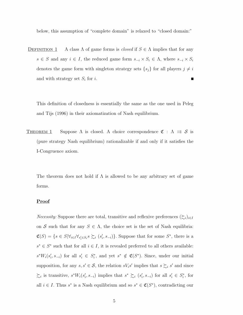
below, this assumption of “complete domain” is relaxed to “closed domain:”

Definition 1 A class Λ of game forms is closed if S ∈ Λ implies that for any

s ∈ S and any i ∈ I, the reduced game form s−i × Si ∈ Λ, where s−i × Si

denotes the game form with singleton strategy sets {sj} for all players j 6= i

and with strategy set Si for i.

This definition of closedness is essentially the same as the one used in Peleg

and Tijs (1996) in their axiomatization of Nash equilibrium.

Theorem 1 Suppose Λ is closed. A choice correspondence C : Λ ⇒ S is

(pure strategy Nash equilibrium) rationalizable if and only if it satisfies the

I-Congruence axiom.

The theorem does not hold if Λ is allowed to be any arbitrary set of game

forms.

Proof

Necessity: Suppose there are total, transitive and reflexive preferences (%i)i∈I

on S such that for any S ∈ Λ, the choice set is the set of Nash equilibria:

C(S) = {s ∈ S|∀i∈I∀s′i∈Si

s %i (s′i, s−i)}. Suppose that for some S∗, there is a

s∗ ∈ S∗ such that for all i ∈ I, it is revealed preferred to all others available:

s∗Wi(s′i, s−i) for all s′i ∈ S∗

i , and yet s∗ /∈ C(S∗). Since, under our initial

supposition, for any s, s′ ∈ S, the relation sVis′ implies that s %i s′ and since

%i is transitive, s∗Wi(s′i, s−i) implies that s∗ %i (s′i, s−i) for all s′i ∈ S∗

i , for

all i ∈ I. Thus s∗ is a Nash equilibrium and so s∗ ∈ C(S∗), contradicting our

5

initial supposition and proving the necessity of I-Congruence.

Sufficiency: Assume that I-Congruence holds. For S ∈ Λ and s ∈ S, let Ssi de-

note the one-player subform with strategy sets {sj} for all j 6= i, and strategy

set Si for player i. For each i ∈ I, let Λi := {Ssi |S ∈ Λ, s ∈ S}. (Note that

by closedness ∅ 6= Λi ⊆ Λ.) We derive, for each i ∈ I, an “individual choice

correspondence” Ci on Λi. For all S ∈ Λi, let

Ci(S) := {x ∈ S|x ∈ C(S) for some S with S = Sxi } (3)

By definition, the revealed preferred relation derived from Ci coincides with

Wi. Therefore, by I-Congruence, Ci coincides with C on Λi. Since I-Congruence

restricted to the one-player games Λi is the same as the Congruence axiom of

Richter (1966), for each i ∈ I there exists a total, transitive, reflexive binary

relation %i on S such that for each S ∈ Λi, the set Ci(S) = C(S) is the set

of %i-maximal elements. We will show that these preferences (pure strategy

Nash equilibrium) rationalize C on Λ.

C(S) are Nash equilibria: Given S ∈ Λ, suppose s′ ∈ C(S). Then, for all i ∈ I,

by the definition of Wi it must be that s′Wis′′ for all s′′ ∈ Ss′

i . Since %i extends

Wi (see Richter (1966)), this implies that for all i ∈ I, s′ %i s′′ for all s′′ ∈ Ss′

i ,

i.e. that s′ is a Nash equilibrium.

all Nash equilibria are chosen by C: Given (S) ∈ Λ, suppose that s′ ∈ S is a

Nash equilibrium, i.e. for all i ∈ I, it holds that s′ %i s′′ for all s′′ ∈ Ss′

i . Since

%i rationalizes Ci = C on Λi, we have s′ ∈ Ci(Ss′

i ) = C(Ss′

i . Then s′Wis′′ for

all s′′ ∈ Ss′

i , and, by I-Congruence, s′ ∈ C(S). Q.E.D.

6

3 Nash equilibrium rationalizability under arbitrary domains

In the previous section we substantially weakened the “complete domain” as-

sumption of the previous literature to “closedness.” In a revealed preference

context even this assumption seems restrictive, and one would like to avoid

any restrictions on the set of game forms observed. Formally this means that

Λ could be an arbitrary set of game forms. While it is possible, even under

arbitrary domains, to characterize Nash rationalizability using revealed pref-

erence conditions, we show in this section that this problem is NP-complete.

That is, any algorithm that decides Nash rationalizability for choice corre-

spondences with arbitrary domains is necessarily very complex computation-

ally. This holds even if there are only two players. It is natural to ask whether

the same complexity arises if there is only a single player. We show that it

does not — the appropriate one player analogue of the Nash rationalizability

problem can be decided in polynomial time.

In this section we assume that the universal strategy spaces Si are finite. Let Λ

be an arbitrary finite set of game forms, i.e. a set of Cartesian product subsets

of 4 S. For each subform S ∈ Λ, we observe the strategy profiles played. We

assume that if there are several strategy profiles which players would be willing

to choose, then we observe all of these as chosen. As before, we ask whether a

given choice correspondence C is pure strategy Nash rationalizable. To simplify

notation, we now require Nash rationalizability by strict preferences. 5 That

is, we ask

4 Recall that S :=∏

i∈I Si.5 All the results below continue to hold if we ask for rationalizability by weak

preferences.

7

Question 2 When can we find total, transitive and asymmetric preferences

(≺i)i∈I on S such that for all S ∈ Λ, the chosen set C(S) is the set of pure

strategy Nash equilibria of (S, (≺i)i∈I), i.e.

s∗ ∈ C(S) ⇐⇒ ∀i ∈ I,∀si ∈ Si, (si, s∗−i) ≺i s∗?

If we can find such preferences, we say that C is (pure strategy Nash equilib-

rium) rationalizable.

It is possible to characterize pure strategy Nash rationalizability for arbi-

trary domains (Galambos, 2004). In addition to deriving revealed preference

relations from chosen strategy profiles (as in section 2), one must also de-

rive revealed preference relations from non-chosen strategy profiles. Suppose,

for example, that a 3 × 3 subform in Λ — involving only two players — is

{s1, s2, s2}× {z1, z2, z3}, and the strategy profile chosen by C is (s1, z1). As in

section 2, we then infer that if C is to be Nash rationalized, it must be that

(s2, z1) ≺1 (s1, z1) and (s3, z1) ≺1 (s1, z1) (4)

(s1, z2) ≺2 (s1, z1) and (s1, z3) ≺2 (s1, z1). (5)

In addition, since (s3, z3) was not chosen, it must also be that

(s3, z3) ≺1 (s2, z3)or (s3, z3) ≺1 (s1, z3) OR (6)

(s3, z3) ≺2 (s3, z2)or (s3, z3) ≺2 (s3, z1).

It is not surprising that deciding Nash rationalizability from a set of such state-

ments could be computationally very complex. It is natural to ask whether

there exists an alternative, not so complex method for deciding rationalizabil-

ity. The main result of this section answers that question in the negative.

8

Theorem 2 The (pure strategy Nash equilibrum) rationalizability problem is

NP-complete.

In fact, we prove a stronger statement: The (pure strategy Nash equilibrum)

rationalizability problem is NP-complete even if we have only two players.

The proof (in Appendix A) is based on a standard technique in the theory of

computational complexity: “polynomially reducing” a problem that is known

to be NP-complete to the given problem. 6

3.1 Supra-semirationalizability

With only one player, the Nash rationalizability problem (as formulated in

section 3) specializes to the classical revealed preference problem with finite

budgets. It is not difficult to show then that rationalizability of a non-empty

valued choice correspondence C : Λ ⇒ S can be decided in polynomial time.

One might conjecture that the complexity of the two-player problem does not

arise with one decision maker because rationalizability can be characterized

without having to use the disjunctive revealed preferred relations (like (6)

above) that are derived from non-chosen points in the multi-player problem.

Somewhat surprisingly, this is only partly true. The statement in (6) has dis-

junctions in two roles. The capitalized “OR” separates two statements, one of

which relates to player 1 only, and the other to player 2 only. This disjunction

corresponds, intuitively, to “player 1 would deviate at (s3, z3) OR player 2

would deviate at (s3, z3).” In each of those two statements, the occurrences of

6 Specifically, we use 3SAT, a version of the satisfiability problem that was shown

to be NP-complete in Cook (1971).

9

the small case “or” separate the different possible deviations of a particular

player. While disjunctions of the first kind (“OR”) clearly cannot occur with

one player, it is possible to formulate the problem for one decision maker so

that disjunctions of the second kind (“or”) can occur. We present such a for-

mulation below, and show that even this more general and intuitively more

complex problem can be decided in polynomial time.

Suppose that one decision maker chooses from finite budgets S ∈ Λ. However,

our observations of her choices are imperfect in the sense that her actual chosen

set is known to be only a subset of the observed set C(S). 7 To determine

whether her choices could be generated by maximizing a preference relation,

we must ask the question: Does there exist a preference relation ≺ on S such

that for each budget S ∈ Λ the ≺-maximal elements are contained in C(S)?

This notion of rationality was labeled supra-semirationality by Matzkin and

Richter (1991). Since we do not know whether an element s ∈ C(S) is actually

chosen or not, we can derive revealed preferred relations only from elements not

in C(S). We know that if s /∈ C(S), some element of C(S) must be preferred

to it. For example, if S = {s1, s2, s3, s4} and C(S) = {s2, s4}, then supra-

semirationalizability of C requires

s1 ≺ s2 or s1 ≺ s4, (7)

s3 ≺ s2 or s3 ≺ s4.

More generally, our “data set” looks like

7 For example, she might choose bundles consisting of three different goods, but we

observe her choice only in two of those goods.

10

s1

0/∈C({s1

0, s1

1, . . . , s1

k1}) (8)

s2

0/∈C({s2

0, s2

1, . . . , s2

k2}) (9)

... (10)

sm0

/∈C({sm0

, sm1

, . . . , smkm}), (11)

where sqr ∈ S for q = 1, . . . ,m and r = 0, . . . , kq. We write the set of direct

revelations as

s1

0C {s1

1, . . . , s1

k1} (12)

s2

0C {s2

1, . . . , s2

k2} (13)

...

sm0

C {sm1

, . . . , smkm}. (14)

The interpretation is that the decision maker strictly prefers some element of

{s11, . . . , s1

k1} to s1

0, and strictly prefers some element of {s2

1, . . . , s2

k2} to s2

0, etc.

It is clear that supra-semirationalizability is equivalent to (12 – 14).

If every alternative appearing in one of the sets on the right hand side in

(12–14) also appeared on the left hand side on some other line, it is clear that

there would exist no rationalization. If there were one, the alternatives that

appear in (12–14) would contain a preference cycle: s10

would be worse than

some alternative on the right in (12), which in turn would appear on the left

on another line and so would be worse than another alternative, which in turn

would appear on the left on another line, and so would be worse than . . . . With

a finite number of alternatives, this would result in a preference cycle. For this

reason, if a set of revelations has the property that all alternatives appearing

on the right also appear on the left, we say that it is an implicit cycle. Thus it

is a necessary condition for rationalizability that the set of revelations contain

no implicit cycle. In separate work on supra-semirationalizability we show that

this condition is also sufficient for rationalizability.

11

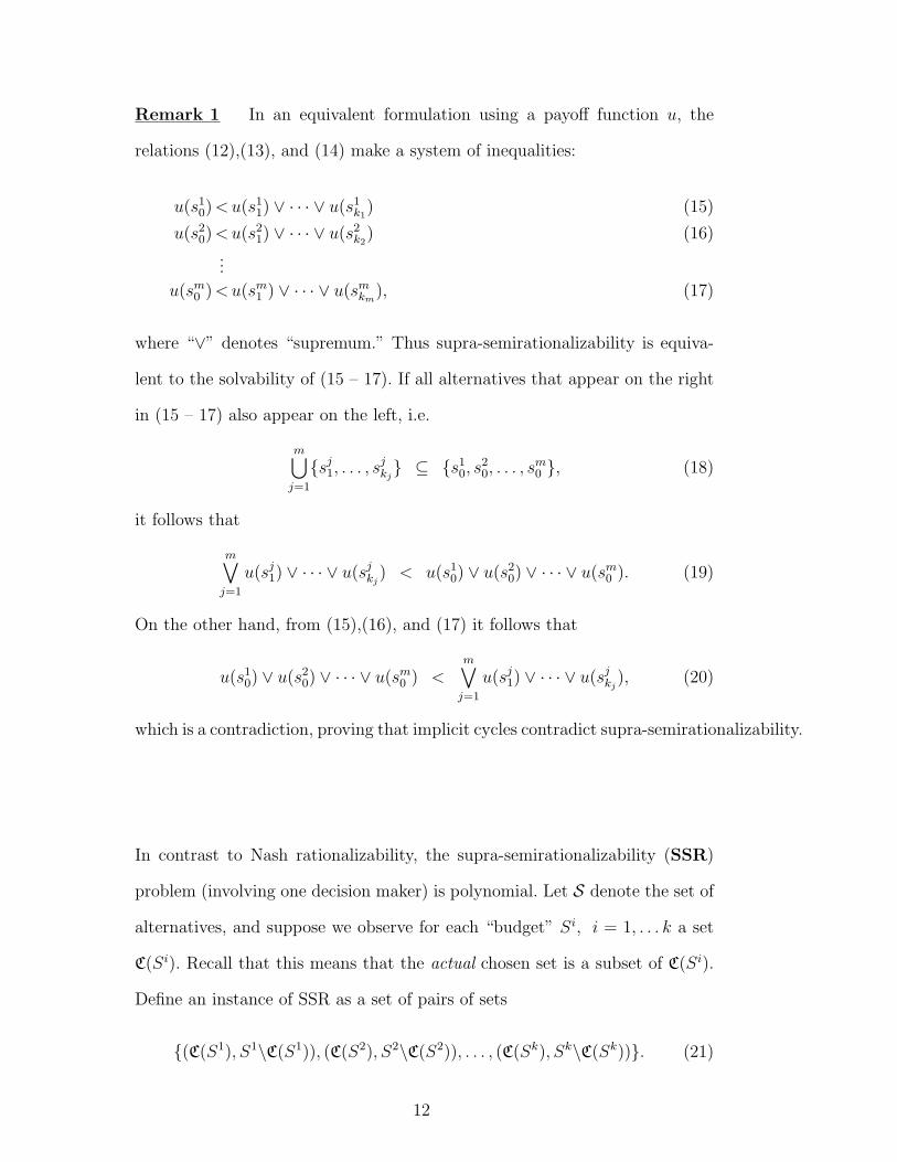
Remark 1 In an equivalent formulation using a payoff function u, the

relations (12),(13), and (14) make a system of inequalities:

u(s1

0) < u(s1

1) ∨ · · · ∨ u(s1

k1) (15)

u(s2

0) < u(s2

1) ∨ · · · ∨ u(s2

k2) (16)

...

u(sm0

) < u(sm1

) ∨ · · · ∨ u(smkm

), (17)

where “∨” denotes “supremum.” Thus supra-semirationalizability is equiva-

lent to the solvability of (15 – 17). If all alternatives that appear on the right

in (15 – 17) also appear on the left, i.e.

m⋃

j=1

{sj1, . . . , s

jkj} ⊆ {s1

0, s2

0, . . . , sm

0}, (18)

it follows that

m∨

j=1

u(sj1) ∨ · · · ∨ u(sj

kj) < u(s1

0) ∨ u(s2

0) ∨ · · · ∨ u(sm

0). (19)

On the other hand, from (15),(16), and (17) it follows that

u(s1

0) ∨ u(s2

0) ∨ · · · ∨ u(sm

0) <

m∨

j=1

u(sj1) ∨ · · · ∨ u(sj

kj), (20)

which is a contradiction, proving that implicit cycles contradict supra-semirationalizability.

In contrast to Nash rationalizability, the supra-semirationalizability (SSR)

problem (involving one decision maker) is polynomial. Let S denote the set of

alternatives, and suppose we observe for each “budget” Si, i = 1, . . . k a set

C(Si). Recall that this means that the actual chosen set is a subset of C(Si).

Define an instance of SSR as a set of pairs of sets

{(C(S1), S1\C(S1)), (C(S2), S2\C(S2)), . . . , (C(Sk), Sk\C(Sk))}. (21)

12

Such a list is a yes-instance if there exists a preference relation on S such that

for each Si, the set C(Si) contains the preference-maximal elements. Otherwise

it is a no-instance.

Theorem 3 The supra-semirationalizability problem can be decided in polyno-

mial time.

Proof

The following algorithm determines in polynomial time whether an instance

of SSR is a yes-instance or a no-instance. By “polynomial time” we mean,

intuitively, that the number of steps in the algorithm is polynomial in the

length of the input string ((21) above, with the finite sets C(Si) and Si\C(Si)

written out element by element).

Algorithm:

1. Let I := {1, . . . , k}. Let Q = ∅.

2. Let q = 1 and r = 1.

3. Scan the sets Si\C(Si), i ∈ I, to check if the qth element of C(Sr) (denote

it by x∗) appears in any of them.

3.1. If it does:

3.1.1. If C(Sr) has q elements and r is the highest index in I, STOP.

3.1.2. If C(Sr) has q elements, let q = 1 and increase r by 1. Go to

step 3.

3.1.3. Increase q by 1 and go to step 3.

3.2. If x∗ does not appear in any Si\C(Si), add it to Q and set x ≺ x∗

for all x ∈ S\Q.

3.3. Scan the sets C(Si), i ∈ I to check if x∗ appears in any of them,

13

and let I ′ := {i ∈ I : x∗ /∈ C(Si)} (note that by the definition of x∗

in step 3, I ′ $ I). If I ′ = ∅, set I = ∅ and STOP. (Note that the

observations with labels in I\I ′ are now supra-semirationalized by

≺.)

3.4. Relabel the pairs (C(Si), Si\C(Si)), i ∈ I ′, with the labels 1, . . . , |I ′|.

Let I := {1, . . . , |I ′|}. Go to step 2.

At every iteration the algorithm either returns to step 2 or 3 or it stops. The

algorithm stops after at most∑k

i=1|C(Si)| iterations. If I 6= ∅ when the al-

gorithm stops, the input choice correspondence is a no-instance. In this case

{(C(Si), Si\C(Si))| i ∈ I} is an implicit cycle, and by the argument on page

11 the input choice correspondence is not rationalizable. If I = ∅ when the

algorithm stops, the input choice correspondence is a yes-instance. In this case

≺ is a partial order on S that supra-semirationalizes the input choice corre-

spondence. 8 It is clear that each step is polynomial in the length of the input,

and so is the number of iterations. Q.E.D.

4 Conclusion

We characterized behavior generated by the pure strategy Nash equilibrium

concept for normal form games under a “closed domain” assumption. Our

characterization is a straightforward extension of classical revealed preference

theory to a multi-agent setting.

8 This can be seen by noticing that indicies are ommitted from I in step 3.3 only

if the corresponding observation is rationalized by the partial order defined so far.

14

Without restrictions on the domain of the choice correspondence, pure strategy

Nash rationalizability is a computationally very complex problem. Specifically,

it is an NP-complete problem even if the number of players is held fixed

(and is two or more). In contrast, the one-player analogue of the problem,

supra-semirationalizability, can be decided in polynomial time. This implies

that the classical revealed preference problem (with finite budgets) and the

Nash rationalizability problem under a “closed domain” can also be decided

in polynomial time.

An interesting question for future research is the role of beliefs in multi-agent

decision making. Since the literature so far has addressed only the Nash equi-

librium solution concept, the role of beliefs has been hidden by the implicit

assumption that agents’ beliefs correspond exactly to the actions taken. If

one were to study behavior generated by other solution concepts that are not

“Nash-like,” such as Pearce-Bernheim rationalizability, the prominent role of

beliefs would become apparent.

Another interesting aspect of this problem is the relationship between the

analyst or observer and the decision making process. In rationalizability for

individual choice problems, it seems clear that the observer and the deci-

sion making process are entirely separate. That is, the analyst is outside the

decision making problem, observing the behavior of the decision maker. In

collective decision making situations, it is conceivable that the analyst is him-

self one of the decision makers. For example, a player in a game, not knowing

the preferences of the other players, might attempt to draw conclusions con-

cerning the plausibility of certain possible outcomes, based on some previous

experiences of games played by the same agents. Analyzing situations of this

kind might lead to interesting applications.

15

A Appendix

Here we prove Theorem 2 of section 3, which states that the Nash ratio-

nalizability problem (NR) is NP-complete. Our proof involves two additional

problems: Nash rationalizability with only two players 9 (NR2), and the classic

problem of determining the satisfiability of a Boolean formula in conjunctive

normal form with three disjuncts in each conjunct (3SAT).

Proof [Theorem 2 ]

We will prove the theorem using polynomial-time reduction, a standard tech-

nique in the theory of computational complexity. We will show that the 3SAT

problem, known to be NP-complete (see Cook (1971) and Garey and Johnson

(1979)), polynomially transforms into the Nash rationalizability problem with

two players (henceforth denoted by NR2), which is a special case of the Nash

rationalizability problem (henceforth denoted by NR). That is, we will con-

struct an algorithm that runs in polynomial time, and, given any instance of

3SAT, produces an instance of NR2 with the property that the NR2 instance

is rationalizable if and only if the 3SAT instance is satisfiable. This will imply

that if there exists a polynomial-time algorithm for deciding NR2, then any

instance of 3SAT can be decided in polynomial time by first polynomially

transforming it into an instance of NR2 and then deciding that in polynomial

time. Since 3SAT is NP-complete, this argument will establish that NR2 is

NP-complete.

NR2: The Nash rationalizability problem with two players can be described

as follows. Let S := {s∗, s∗, s0, s1, s2, s3, . . . } be the set of potential actions of

9 I.e. the same two players are involved in every observed subform.

16

player 1 (in any subform a finite subset of this will be player 1’s action space).

Let Z := {z∗, z∗, z0, z1, z2, . . . } be the set of potential actions of player 2 (in

any subform a finite subset of this will be player 2’s action space). An instance

of NR2 consists of a choice function on a finite set of finite subforms of S×Z.

For example, the following instance of NR2 encodes a choice function on two

subforms.

({s0, s1, s2} × {z0, z1}, s2z1) , ({s0, s4, s5} × {z0, z2}, s4z0) (A.1)

The first subform is {s0, s1, s2}× {z0, z1}, and the (only) observed outcome is

(s2, z1). In general, an instance of NR2 consists of a list of subform–outcome

pairs of the form (A × B, ab), where A ⊂ S, B ⊂ Z and a ∈ A, b ∈ B. An

instance of NR2 is a yes-instance if the corresponding choice function is (pure

strategy Nash equilibrium) rationalizable, and it is a no-instance if it is not.

A polynomial-time algorithm for NR2 is a polynomial-time algorithm that

returns, for any given instance of NR2, a yes if and only if it is a yes-instance.

Below we will show that if there exists a polynomial-time algorithm for NR2,

then there exists a polynomial-time algorithm for 3SAT, which proves that

NR2 is NP-complete. 10

3SAT: Suppose that X = {x1, x2, . . . , xm} is a set of Boolean variables and

X = {x1, . . . , xm} is the set of their negations. For any truth assignment

T : X → {t, f}, we define for x ∈ X the extension of T by T (x) = t if, and

only if T (x) = f. The set X∗ := X ∪ X is the set of literals. A subset C of

X∗ is a clause. Suppose a set {C1, . . . , Ck} of clauses is given. A truth assign-

ment T : X → {t, f} satisfies {C1, . . . , Ck} if for every clause Ci there exists

10 It is clear that NR2 is in the class NP: given an instance of NR2 and prefer-

ence relations for every player, it can be checked in polynomial time whether the

preferences Nash rationalize the given choice function.

17

x ∈ Ci with T (x) = t. A set of clauses is satisfiable if there exists a truth

assignment that satisfies it. We can now state 3SAT: Given an arbitrary finite

set of clauses with exactly three elements in every clause, does there exist a

satisfying truth assignment? 3SAT is known to be NP-complete (see Garey

and Johnson (1979)).

3SAT → NR2: We now define the polynomial-time transformation men-

tioned at the beginning of the proof. That is, we define a polynomial-time

algorithm that takes any instance of 3SAT as its input, and produces an in-

stance of NR2 that is rationalizable if and only if the input 3SAT instance is

satisfiable. Suppose we are given an arbitrary instance of 3SAT:

V ={

{v1

1, v2

1, v3

1}, {v1

2, v2

2, v3

2}, · · · , {v1

l , v2

l , v3

l }}

, (A.2)

where vij ∈ X∗. Suppose w.l.o.g. that the set of variables that appear in V is

{x1, . . . , xk}. We will construct an instance of NR2 for V , using the actions

s∗, s∗, s0, s1, . . . , sk for player 1, and the actions z∗, z

∗, z0, z1, . . . , zk for player

2.

Informal description of the construction: For every clause, we construct

a game form where player 1’s action set is s0, s∗, and all si such that xi appears

in the clause and is not negated; player 2’s action set is z0, z∗, and all zi such

that xi appears in the clause and is negated. The (unique) outcome for this

game form is (s∗, z∗). We will construct these game forms in such a way that

rationalizing (s∗, z∗) as a Nash equilibrium will always be possible (and very

simple), and it will also be possible (and simple) to rationalize all other points

except (s0, z0) as not Nash equilibria. Thus rationalizability will boil down to

being able to assign preferences in such a way that (s0, z0) is not a Nash equilib-

rium, and this will be possible if, and only if, the clause on which the game form

was based is satisfied. Satisfying all clauses simultaneously will be possible if,

18

and only if, the set of games constructed according to the above description

can be simultaneously rationalized. Using an example, I will present further

details of the construction, and then I will proceed to a general description.

Suppose the variables appearing in an instance of 3SAT are x1, x2, x3, x4, x5,

and one particular clause is {x1, x2, x3}. Following the above described con-

struction, we have a subform–outcome pair ({s0, s1, s3, s∗}×{z0, z2, z

∗}, s∗z∗).

We will add two additional subform–outcome pairs that will imply that player

1 prefers (s0, z0) to (s∗, z0) and that player 2 prefers (s0, z0) to (s0, z∗). Ra-

tionalizability will boil down to finding preferences for the players such that

either player 1 prefers (s1, z0) to (s0, z0), or player 1 prefers (s3, z0) to (s0, z0),

or player 2 prefers (s0, z2) to (s0, z0). The first of these will correspond to set-

ting x1 true, the second will correspond to setting x3 true, and the third will

correspond to setting x2 false. This procedure, however, may lead us to assign

preferences implying both that a variable xi is true and that it is false. In the

example just described, we might rationalize (s0, z0) not being a Nash equi-

librium by assigning player 2 a preference of (s0, z2) over (s0, z0), which would

correspond to setting x2 false. At the same time, we might rationalize (s0, z0)

not being a Nash equilibrium in another game form by assigning player 1 a

preference of (s2, z0) over (s0, z0), which would correspond to setting x2 true.

To prevent this, we construct a “module” of subform–outcome pairs (denoted

below by Γ2) that will be rationalizable, but only if exactly one of the above

two possibilities hold: either player 2 prefers (s0, z2) to (s0, z0), or player 1

prefers (s2, z0) to (s0, z0), but not both (see Figure A.1).

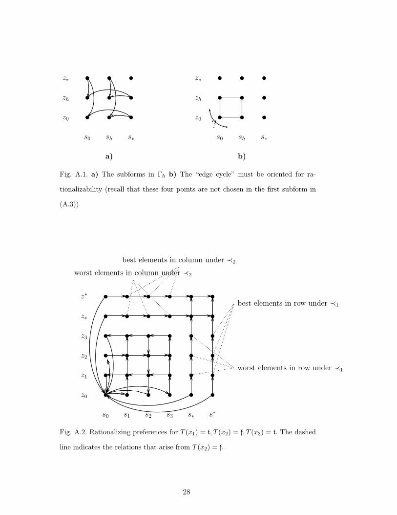
Detailed description of the construction: First we construct a set of

games for every variable that is negated in some clause in V . That is, sup-

pose {v1j , v

2j , xh} ∈ V . Then we construct Γh, which consists of the following

subform–outcome pairs:

19

({s0, sh, s∗} × {z0, zh, z∗}, s∗z∗) (A.3)

({s0} × {zh, z∗}, s0zh)

({s0} × {z0, z∗}, s0z0)11

({sh} × {zh, z∗}, shzh)

({sh} × {z0, z∗}, shz0)

({sh, s∗} × {z0}, shz0)

({s0, s∗} × {z0}, s0z0)11

({sh, s∗} × {zh}, shzh)

({s0, s∗} × {zh}, s0zh)

Figure A.1 illustrates this set of subform–outcome pairs. For transparency, the

first pair in (A.3) is not shown (and, given the other eight subform–outcome

pairs in the list, its rationalizability will depend only on orienting the edge

cycle in Figure A.1 b)). Each of the remaining eight involve only one player,

and only two points, and so each has one revealed preference implication:

the point chosen is preferred to the one not chosen. Figure A.1 a) shows the

resulting eight such implications, with the arrows pointing to the preferred

point. For example, ({s0}×{zh, z∗}, s0zh) is shown as an arrow pointing from

(s0, z∗) to (s0zh).

Now we transform the 3SAT instance V into an instance of NR2 as follows.

1. Replace every clause of the form {xe, xf , xg} with

({s0, se, sf , sg, s∗} × {z0, z

∗}, s∗z∗). (A.4)

2. Replace every clause of the form {xe, xf , xg} with

({s0, se, sf , s∗} × {z0, zg, z

∗}, s∗z∗) (A.5)

and Γg (see (A.3) for the definition of the nine subform–outcome pairs in

11 Note that this is independent of h, so this subform–outcome pair could be included

only once, not for every variable xh that is negated in some clause.

20

Γh for h = 1, . . . , k).

3. Replace every clause of the form {xe, xf , xg} with

({s0, se, s∗} × {z0, zf , zg, z

∗}, s∗z∗) (A.6)

and Γg and Γf .

4. Replace every clause of the form {xe, xf , xg} with

({s0, s∗} × {z0, ze, zf , zg, z

∗}, s∗z∗) (A.7)

and Γg, Γf and Γe.

5. Add the following subform–outcome pairs:

({s0} × {z0, z∗}, s0z0), ({s0, s

∗} × {z0}, s0z0). (A.8)

The resulting instance of NR2 will be denoted by NRV .

In the worst case, all variables that appear in V are distinct and are negated,

which gives l · 30 subform–outcome pairs, i.e. the input size is increased by a

multiplicative factor. The transformation involves only replacing each clause

by at most 30 subform–outcome pairs, as described above, and so it runs in

polynomial time (in fact in linear time).

V satisfiable ⇐⇒ NRV Nash rationalizable: Now we must show that

the polynomial transformation V 7→ NRV constructed above has the property

mentioned at the beginning of the proof: V is satisfiable if and only if NRV

is Nash rationalizable.

⇐ First, suppose NRV is Nash rationalizable. Let 12 Sk := {s∗, s∗, s0, s1, . . . , sk}

and Zk := {z∗, z∗, z0, z1, . . . , zk}, and denote the players’ rationalizing pref-

erences on Sk × Zk by ≺1, and ≺2. Define, for each variable xi with i ∈

12 Recall that V involves the variables x1, . . . , xk.

21

{1, 2, . . . , k} (recall that these are exactly the variables that appear in V ) a

truth assignment:

T≺(xi) = t ⇐⇒ s0z0 ≺1 siz0. (A.9)

Consider a clause of the form {xe, xf , xg}. Since NRV contains (see (A.4) and

(A.8))

({s0, se, sf , sg, s∗} × {z0, z

∗}, s∗z∗), (A.10)

({s0} × {z0, z∗}, s0z0),

({s0, s∗} × {z0}, s0z0),

and since s0z0 is not a Nash equilibrium in the first subform, but it is an

equilibrium in the second and the third, it must be that

[s0z0 ≺1 sez0] or [s0z0 ≺1 sfz0] or [s0z0 ≺1 sez0]. (A.11)

Under T≺ this means that {xe, xf , xg} is satisfied.

Now consider a clause of the form {xe, xf , xg}. It is easy to see that if ≺1, and

≺2 rationalize NRV , then it follows from the construction of Γg that either

s0zg ≺2 s0z0 holds, or sgz0 ≺1 s0z0 holds, but not both. 13

If sgz0 ≺1 s0z0, then by definition T≺(xg) = f, so {xe, xf , xg} is satisfied. If,

on the other hand, s0z0 ≺1 sgz0, then s0zg ≺2 s0z0 holds (the edge cycle in Γg

must be oriented), and since s0z0 is not a Nash equilibrium in ({s0, se, sf , s∗}×

{z0, zg, z∗}, s∗z∗) (see (A.5)), it must be that either s0z0 ≺1 sez0 or s0z0 ≺1

sfz0. Then, by the definition of T≺, either T≺(xe) = t or T≺(xf ) = t, and so

{xe, xf , xg} is satisfied.

13 In fact, Γg is constructed so that it is rationalizable if and only if the “edge cycle”

indicated by a dashed line in Figure A.1 b) is oriented in one direction or the other.

22

The situation for clauses of the type {xe, xf , xg} and {xe, xf , xg} is analogous,

and these clauses will also be satisfied by T≺. Thus the truth assignment T≺

satisfies V .

⇒ To prove the converse, suppose that V is satisfied by a truth assignment

T . We will describe rationalizing (non-total) preference relations ≺1 on Sk and

≺2 on Zk, and we will show that they are acyclic. 14 Then extensions of these

orders to total orders will also rationalize NRV . First we define player 1’s pref-

erences. The example in Figure A.2 illustrates the construction of rationalizing

preferences (for both players).

1. For z ∈ Zk\{z0}, let (s∗, z) be the best element in the row Sk×{z} under

≺1. (In fact, for simplicity, we may order the points in the rows Sk ×{z∗}

and Sk × {z∗} as shown in figure A.2.)

2. In the row Sk × {z0} let (s∗, z0) be the worst element under ≺1.

3. For z ∈ Zk\{z∗, z∗, z0}, let (s∗, z) be the worst element in the row Sk×{z}

under ≺1.

4. In the row Sk × {z0} let (s∗, z0) be worse than any other point except

(s∗, z0) (which we have already defined to be the bottom element in that

row).

5. In the row Sk ×{z∗} let (s∗, z∗) be the second best element under ≺1 (in

step 1. we defined (s∗, z∗) as the best element in this row).

6. For all i ∈ {1, 2, . . . , k} such that T (xi) = t, let s0z0 ≺1 siz0 and

(sk, zi) ≺1 (sk−1, zi) ≺1 · · · ≺1 (s1, zi) ≺1 (s0, zi), (A.12)

14 Recall that Sk := {s∗, s∗, s0, s1, . . . , sk} and Zk := {z∗, z

∗, z0, z1, . . . , zk}.

23

and for all i ∈ {1, 2, . . . , k} such that T (xi) = f, let siz0 ≺1 s0z0 and

(s0, zi) ≺1 (s1, zi) ≺1 · · · ≺1 (sk−1, zi) ≺1 (sk, zi). (A.13)

The preferences ≺2 for player 2 are defined symmetrically — one can just

exchange the roles of “s” and “z” in the preceding definition, and substitute

≺2 for ≺1 and “column” for “row” — except for the crucial step 6., which

becomes:

6’. For all i ∈ {1, 2, . . . , k} such that T (xi) = t, let s0zi ≺2 s0z0 and

(si, z0) ≺2 (si, z1) ≺2 · · · ≺2 (si, zk−1) ≺2 (si, zk), (A.14)

and for all i ∈ {1, 2, . . . , k} such that T (xi) = f, let s0z0 ≺2 s0zi and

(si, zk) ≺2 (si, zk−1) ≺2 · · · ≺2 (si, z1) ≺2 (si, z0). (A.15)

One can easily verify that the above defined preferences are acyclic. Since we

defined relations only on rows and columns, we can check acyclicity for each

row and for each column separately. In the row Sk × {z0} and in the column

{s0} ×Zk all relations involve the point (s0, z0), and so there is no possibility

of a cycle. In the rows Sk × {z∗} and Sk × {z∗} and in the columns {s∗} ×Zk

and {s∗} × Zk it is again clear that ≺1 and ≺2 have no cycles; in fact, we

can define preferences on these rows and columns as shown in Figure A.2. As

to the remaining rows and columns, we will verify acyclicity on just one —

preferences on the others are defined very similarly. Consider the row Sk×{zi}

(where 0 < i ≤ k). The point (s∗, zi) is the best element in that row, (s∗, zi)

is the worst, and the remaining are ordered linearly — i.e., the entire row is

ordered linearly.

It remains to show that these preferences do, in fact, rationalize all the subform–

24

outcome pairs in NRV . It is immediate that the sets of subform–outcome

pairs Γi (for i = 1, . . . , k) are rationalized by these preferences (that is,

the outcome (s∗, z∗) is a Nash equilibirum, and at any other profile either

player 1 prefers to deviate under ≺1 or player 2 prefers to deviate under ≺2).

Checking that the other subform–outcome pairs (A.4–A.8) are also rational-

ized by ≺1 and ≺2 is also routine. For example, consider one of the type

defined in (A.5): ({s0, se, sf , s∗} × {z0, zg, z

∗}, s∗z∗). Under ≺1 and ≺2, the

profile (s∗, z∗) is clearly a Nash equilibrium. The profiles on the same row

or column as (s∗, z∗) are not Nash equilibria, because they are dominated by

(s∗, z∗). The profile (s0, z0) is not a Nash equilibrium because the truth as-

signment T (based on which ≺1,≺2 were defined) is satisfied, and thus either

(s0, z0) ≺1 (se, z0) or (s0, z0) ≺1 (sf , z0) holds (by step 6. in the definition of

≺1), or (s0, z0) ≺2 (s0, zg) holds (by step 6’. in the definition of ≺2). The re-

maining points are not Nash equilibria because either player 1 would deviate

to his s∗ strategy, or player 2 would deviate to her z∗ strategy (or both).

We have shown that our polynomial transformation produces a Nash ratio-

nalizable instance of NR2 if and only if the input 3SAT instance is satisfiable.

Thus if an algorithm could decide any instance of NR2 in polynomial time,

then any instance V of 3SAT could be be decided in polynomial time by first

using our algorithm to produce NRV in polynomial time, and then deciding

NRV in polynomial time. Since 3SAT is NP-complete, this proves that NR2

is NP-complete. Q.E.D.

25

References

Carvajal, A., Ray, I., Snyder, S., February 2004. Equilibrium behavior in mar-

kets and games: testable restrictions and identification. Journal of Mathe-

matical Economics 40 (1-2), 1–40.

Cook, S. A., 1971. The complexity of theorem-proving procedures. In: Pro-

ceedings of the third annual ACM symposium on Theory of computing.

Association for Computing Machinery, pp. 151–158.

Du, D.-Z., Ko, K.-I., 2000. Theory of Computational Complexity. Discrete

Mathematics and Optimization. John Wiley & Sons, Inc.

Galambos, A., 2004. Revealed preference in game theory. Ph.D. thesis, Uni-

versity of Minnesota.

Garey, M. R., Johnson, D. S., 1979. Computers and Intractability. W.H. Free-

man and Company.

Houthakker, H. S., May 1950. Revealed preference and the utility function.

Economica NS 17 (66), 159–174.

Matzkin, R. L., Richter, M. K., 1991. Testing strictly concave rationality.

Journal of Economic Theory 53, 287–303.

Peleg, B., Tijs, S. H., 1996. The consistency principle for games in strategic

form. International Journal of Game Theory 25, 13–34.

Ray, I., Snyder, S., 2003. Observable implications of Nash and subgame-perfect

behavior in extensive games. Tech. Rep. 2, Department of Economics, Brown

University.

Ray, I., Zhou, L., 2001. Game theory via revealed preferences. Games and

Economic Behavior 37, 415–424.

Richter, M. K., 1966. Revealed preference theory. Econometrica 34, 635–645.

Richter, M. K., 1971. Rational choice. In: Chipman, J. S., Hurwicz, L., Richter,

26

M. K., Sonnenschein, H. (Eds.), Preferences, Utility, and Demand. Harcourt

Brace Jovanovich, pp. 635–645.

Richter, M. K., 1975. Rational choice and polynomial measurement theory.

Journal of Mathematical Psychology 12, 99–113.

Samuelson, P. A., 1938. A note on the pure theory of consumer’s behaviour.

Economica 5, 61–71.

Sprumont, Y., 2000. On the testable implications of collective choice theories.

Journal of Economic Theory 93, 205–232.

Yanovskaya, E., 1980. Revealed preference in non-cooperative games. Mathe-

matical Methods in the Social Sciences 24 (13), in Russian.

27

z∗

zh

z0

s0 sh s∗

a)

z∗

zh

z0

s0 sh s∗

b)

?

Fig. A.1. a) The subforms in Γh b) The “edge cycle” must be oriented for ra-

tionalizability (recall that these four points are not chosen in the first subform in

(A.3))

z∗

z∗

z3

z2

z1

z0

s0 s1 s2 s3 s∗ s∗

best elements in column under ≺2

worst elements in column under ≺2

best elements in row under ≺1

worst elements in row under ≺1

Fig. A.2. Rationalizing preferences for T (x1) = t, T (x2) = f, T (x3) = t. The dashed

line indicates the relations that arise from T (x2) = f.

28