RF FUNDAMENTALS for the

INTERNET of THINGS

BRENT McADAMS November, 2017

Executive Summary

Demystifying RF for IoT Deployments

With the Internet of Things (IoT) and the emergence of the Industrial Internet of Things (IIoT), a

surge of innovation is occurring across the industry that connects an ecosystem of sensors,

devices and equipment to a network that promises to improve asset utilization, enhance

process efficiency and boost productivity.

With the estimated number of connected “things” expected to reach over 25 billion by

2020i, this provides an opportunity to change the way business is done.

The IoT Ecosystem, as depicted below in Figure 1, consists of Sensors, Gateways, Infrastructure, and

of course, the flashy part of the IoT Ecosystem, Big Data and Analytics. A speaker at a recent IoT

conference summed it up best with the statement “Big Data will be Big!”. The modeling of data

supporting predictive analytics, whether it resides in the cloud or at the edge, gives organizations the

ability to quickly diagnose and troubleshoot not only their sensor networks from a predictive

maintenance perspective but also their operations, reducing excess use of energy and/or raw

materials.

Figure 1. IoT Ecosystem

While the Ecosystem can be hardwired, typically, a hybrid approach is utilized. This includes

wireless sensor networks (WSN) and much of the network infrastructure through highspeed,

broadband links. Even though Radio Frequency (RF) technology is a part of our everyday lives and

in terms of IIoT, has been adopted for decades in some of the harshest conditions, wireless

technology is still viewed by many as magic. Arthur C. Clarke was a brilliant futurist and writer, but

he is best known for one of his laws being “Any sufficiently advanced technology is

indistinguishable from magic”ii. Certainly, wireless (or RF) communications falls within that law. The

purpose of this paper is to help demystify the subject as regardless of the RF Technology used in IoT

deployments, the same core principles apply.

FOUNDATION

In the simplest of terms, wireless transmissions are radio frequency (RF) signals which travel based on

behaviors called propagation characteristics. RF radiates from an antenna on the transmitter end

and is received by an antenna on the receiver end. The actual data being carried is modulated on

one end, transmitted over the air, and demodulated on the other end. The RF signal’s propagation

characteristics are dictated by frequency, wavelength, and amplitude.

Depending on the technology and the part of the world the system is being deployed, regulatory

bodies for that country will govern the frequencies that can be used. For instance, in the U.S., the

Federal Communications Commission (FCC) allocated what is known as the Industrial, Scientific, and

Medical (ISM) Band which allows license free operation in the 900MHz, 2.4GHz and 5.8GHz bands.

However, other countries may use 900MHz for their national cellular band or even over the air

television. In addition, there are also licensed bands used below 900MHz and above 5.8GHz.

Regardless of the band selected, the same propagation characteristics mentioned earlier apply.

Using 900MHz as an example, which is one of the more common IoT bands, the typical operation is

from 902-928 MHz. Hertz (Hz) simply means frequency or cycles per second where the preceding “M”

is a prefix meaning Mega, denoting a factor of one Million. Therefore, at 900 MHz, the frequency is

900 Million (900,000,000) cycles per second. Wi-Fi most commonly uses 2.4 GHz and 5.8 GHz, where

the G is a prefix meaning Giga, denoting a factor of one Billion. Therefore, the frequency is 2.4 Billion

(2,400,000,000) and 5.8 Billion (5,800,000,000) cycles per second respectively.

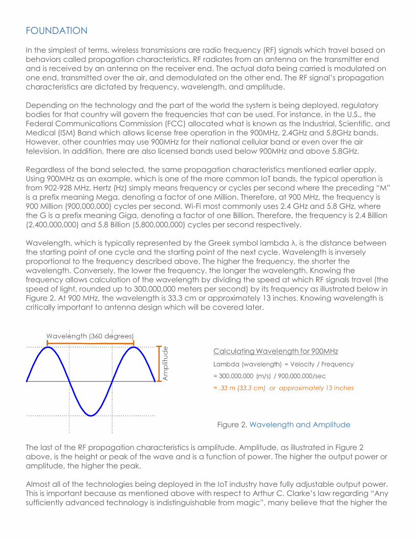
Wavelength, which is typically represented by the Greek symbol lambda λ, is the distance between

the starting point of one cycle and the starting point of the next cycle. Wavelength is inversely

proportional to the frequency described above. The higher the frequency, the shorter the

wavelength. Conversely, the lower the frequency, the longer the wavelength. Knowing the

frequency allows calculation of the wavelength by dividing the speed at which RF signals travel (the

speed of light, rounded up to 300,000,000 meters per second) by its frequency as illustrated below in

Figure 2. At 900 MHz, the wavelength is 33.3 cm or approximately 13 inches. Knowing wavelength is

critically important to antenna design which will be covered later.

Figure 2. Wavelength and Amplitude

The last of the RF propagation characteristics is amplitude. Amplitude, as illustrated in Figure 2

above, is the height or peak of the wave and is a function of power. The higher the output power or

amplitude, the higher the peak.

Almost all of the technologies being deployed in the IoT industry have fully adjustable output power.

This is important because as mentioned above with respect to Arthur C. Clarke’s law regarding “Any

sufficiently advanced technology is indistinguishable from magic”, many believe that the higher the

output power, the better. However, in some cases, higher output power just increases the overall

noise floor and can create self-interference. Although, in other cases, higher output power is needed

just to overcome ambient noise. Regarding output power, RF power is measured by two units on two different scales. The first is a

linear scale using milliwatts (mW). On the linear scale, the reference point is zero but does not reveal

gain or loss in relation to the whole. The second, is a relative scale, measured in decibels (dB) where

the reference point is the measurement itself. dB is nothing more than a ratio expressed on a

logarithmic scale and gets very confusing because it is completely relative, with no reference but

does reveal gain or loss in relation to the whole. Using dB for power measurement simplifies our

calculations and is what allows us to add and subtract our gains and losses.

A couple of the most common examples of referenced dB values are dBm and dBi. dBm is absolute

power measured relative to 1mW whereas, dBi is antenna gain referenced to a hypothetical,

perfect isotropic radiator. System gain and fade margin will be discussed later in this document

which will provide some clarity into why dB is important. For now, perhaps the most important thing to

remember in the world of RF is the rule of 3’s and 10’s. If you can remember five basic steps, you can

perform any RF math calculation. The five basic steps are as follows:

SENSITIVITY

When evaluating wireless technology, the sensitivity specification is just as important as the raw

output power. In our everyday conversations, we know that it is just not about how loud someone

can talk but also how well we can hear and more importantly, be able to understand what they are

saying. Sensitivity provides this “hearing” specification. Receiver sensitivity is the lowest power level at

which the receiver can detect an RF signal and just like being able to understand a conversation,

demodulate the data.

Usually, there is a Bit Error Rate (BER) specification following the receiver sensitivity specification. It is

typically expressed as 10 to a negative power and is essentially, the ability to understand what the

other device is transmitting. For example, a bit error rate of 10-4 means that the probability of a bit

error will occur for every 10,000 bits transmitted.

As with output power, the rule of 3s and 10s also apply here. When comparing a receiver sensitivity

specification of -110dBm to that of one with a -107dBm, the first thought is that there is only a

difference of 3dB. However, the receiver with the -110dBm specification can hear signals that are

half as strong as the receiver with the -107dBm specification. Because receive sensitivity indicates

how faint a signal can be successfully received, the lower the power level, the better. This means

that the larger the absolute value of the negative number, the better the receive sensitivity.

0dBm = 1mW (starting point)

30dBm = 1W

Increase by 3dBm, power in mW doubles

Decrease by 3dBm, power in mW is halved

Increase by 10 dBm, power in mW is multiplied by 10

Decrease by 10 dBm, power in mW is divided by 10

PRACTICAL APPLICATION

With some of the fundamentals behind us, let’s make practical use of the information as well as

introducing new terminology and concepts. Regardless of the wireless technology being

implemented, link budgets are key in determining whether a system will work. Link budgetiii accounts

for all of the gains and losses from the transmitter, through the medium (free space, cable,

waveguide, fiber, etc.) to the receiver in a telecommunication system. It accounts for the

attenuation of the transmitted signal due to propagation, as well as the antenna gains and

miscellaneous losses. A simple link budget equation looks like this:

Received Power (dB) = Transmitted Power (dB) + Gains (dB) − Losses (dB)

The image below in figure 3 helps to explain this concept and will certainly provide some insight as to

why some wireless links work and others do not. Starting from the transmitter, we will walk through

each step of the wireless link and discuss each item as numbered in Figure 3, providing a simplistic

hypothetical example for each variable on a system operating at 900MHz, completing the Link

Budget calculation in step 9.

Figure 3. Link Budget

Transmitter Output Power – The transmitter output power will be based on the technology

being deployed and the country it is being deployed in. With intrinsically safe, battery-

powered wireless sensor networks, minimizing energy use is a primary goal to maximize

battery life. As such, output power could be as low as 10 dBm (or 10mW). However, for

other systems such as licensed radio systems, output power can be significantly higher.

Hypothetical Example: 30dBm (1W)

Transmitter Loss - from the RF connector of the transmitter to the antenna, the system will

experience losses from the coaxial cable as well as insertion lossiv resulting from jumpers,

adapters/connectors, lightning arrestors, etc. It is very important when remote mounting

an antenna to consult the manufacturer’s specifications for the coaxial cable being

used. Misapplication of the improper cable can result in a loss that will prevent the system

from working properly. As an example, LMR400 low loss cable will experience a loss of

3.9dB/100 ft. @ 900 MHz whereas using the same cable @ 2.4 GHz will result in a loss of

6.8dB/100 ft.v

Hypothetical Example: 4.3 dB of loss (3.9dB from 100’ LMR400 and 2 connectors at .2dB

each)

Antenna Gain – Antennas are a complete subject in itself and perhaps one of the most

complicated aspects of an RF system. There have been numerous books published on

antenna theory and design that go into explicit detail. However, an antenna is an

electromagnetic radiator converting electrical currents to radio waves at the

transmitting end and back to electrical currents on the receiving end.

The most common types of antennas are omni-directional and directional antennas.

Omni-directional antennas radiate its energy in a 360° pattern whereas a directional

antenna will focus its energy in one direction. In point-to-multipoint systems, omni-

directional antennas are typically used at the gateway (or access point) and repeater

sites whereas the remote sites use directional antennas, especially in those applications

where remote transmitters are located a significant distance from the gateway.

All antennas have a gain specification typically expressed in dBi which as mentioned

previously is referenced to a hypothetical isotropic antenna. In directional antennas, as

shown in Figure 4, as gain increases, so does the directionality.

Figure 4. Antenna Gain

The energy radiated from the antenna, identified above in Figure 3 as EIRP, is the

Effective Isotropic Radiated Power and accounts for all the gains and losses on that end

of the system. In our hypothetical example thus far, the transmitter has an output power

of 30dBm, the losses in coax and connectors are 4.3dB, and shown below, we will use an

antenna with a gain of 3dBi. Therefore, the EIRP is 28.7dBm.

Hypothetical Example: 3 dBi of gain

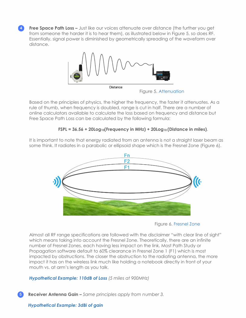
Free Space Path Loss – Just like our voices attenuate over distance (the further you get

from someone the harder it is to hear them), as illustrated below in Figure 5, so does RF.

Essentially, signal power is diminished by geometrically spreading of the waveform over

distance.

Figure 5. Attenuation

Based on the principles of physics, the higher the frequency, the faster it attenuates. As a

rule of thumb, when frequency is doubled, range is cut in half. There are a number of

online calculators available to calculate the loss based on frequency and distance but

Free Space Path Loss can be calculated by the following formula:

FSPL = 36.56 + 20Log10(Frequency in MHz) + 20Log10 (Distance in miles).

It is important to note that energy radiated from an antenna is not a straight laser beam as

some think. It radiates in a parabolic or ellipsoid shape which is the Fresnel Zone (Figure 6).

Figure 6. Fresnel Zone

Almost all RF range specifications are followed with the disclaimer “with clear line of sight”

which means taking into account the Fresnel Zone. Theoretically, there are an infinite

number of Fresnel Zones, each having less impact on the link. Most Path Study or

Propagation software default to 60% clearance in Fresnel Zone 1 (F1) which is most

impacted by obstructions. The closer the obstruction to the radiating antenna, the more

impact it has on the wireless link much like holding a notebook directly in front of your

mouth vs. at arm’s length as you talk.

Hypothetical Example: 110dB of Loss (5 miles at 900MHz)

Receiver Antenna Gain – Same principles apply from number 3.

Hypothetical Example: 3dBi of gain

Receiver Loss - Same principles apply from number 4.

Hypothetical Example: 4.3dB of loss

Received Signal Strength – this is the received signal strength at the Receiver after all the

gains and losses (Free Space Path loss of -110 dBm plus 27.4dB of system gain).

Hypothetical Example: -82.6dBm (the expected received strength level)

Receiver Sensitivity –Receiver sensitivity, as covered earlier, is the threshold or lowest

power level at which the receiver can detect an RF signal. Having a received signal

strength (from number 7) equal to or less than the receiver is not desirable and will not

produce a reliable link. Therefore, contingency or margin must be factored in and will be

covered in number 9.

Hypothetical Example: -110dBm (Receiver Sensitivity, specified from manufacturer)

Fade Margin – Finally, that contingency mentioned above is just how much margin

(expressed in dB) there is between the received signal and the receiver sensitivity. This

margin can help overcome the attenuation through obstacles, attenuation from rain and

atmospheric conditions as well as challenges faced with terrain.

Like most RF parameters, there are differing opinions of recommended fade margins.

However, designing systems with 20 dB of margin will leave you with a robust system and a

high degree of reliability.

Based on the information supplied above, Figure 7 provides a summary of the Hypothetical

Example and our Fade Margin.

Figure 7. Calculated Link Budget

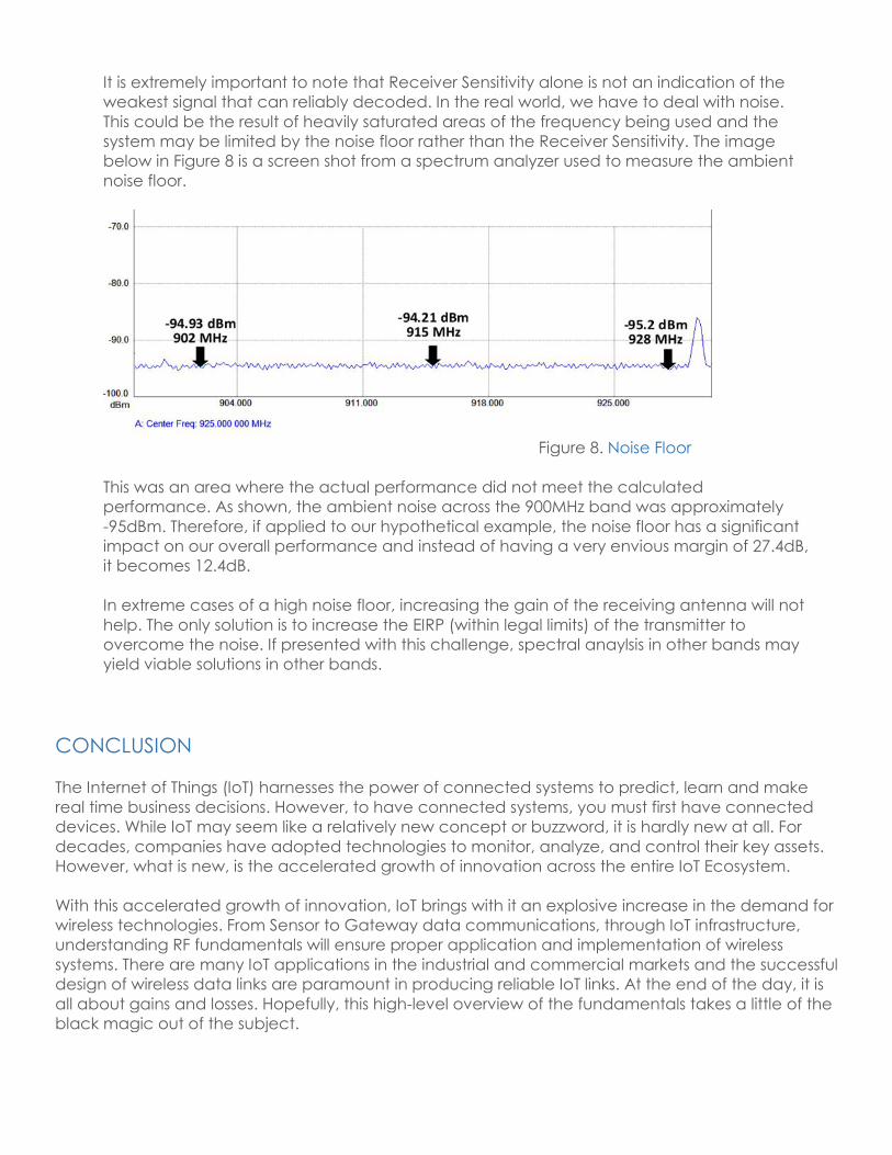
It is extremely important to note that Receiver Sensitivity alone is not an indication of the

weakest signal that can reliably decoded. In the real world, we have to deal with noise.

This could be the result of heavily saturated areas of the frequency being used and the

system may be limited by the noise floor rather than the Receiver Sensitivity. The image

below in Figure 8 is a screen shot from a spectrum analyzer used to measure the ambient

noise floor.

Figure 8. Noise Floor

This was an area where the actual performance did not meet the calculated

performance. As shown, the ambient noise across the 900MHz band was approximately

-95dBm. Therefore, if applied to our hypothetical example, the noise floor has a significant

impact on our overall performance and instead of having a very envious margin of 27.4dB,

it becomes 12.4dB.

In extreme cases of a high noise floor, increasing the gain of the receiving antenna will not

help. The only solution is to increase the EIRP (within legal limits) of the transmitter to

overcome the noise. If presented with this challenge, spectral anaylsis in other bands may

yield viable solutions in other bands.

CONCLUSION

The Internet of Things (IoT) harnesses the power of connected systems to predict, learn and make

real time business decisions. However, to have connected systems, you must first have connected

devices. While IoT may seem like a relatively new concept or buzzword, it is hardly new at all. For

decades, companies have adopted technologies to monitor, analyze, and control their key assets.

However, what is new, is the accelerated growth of innovation across the entire IoT Ecosystem.

With this accelerated growth of innovation, IoT brings with it an explosive increase in the demand for

wireless technologies. From Sensor to Gateway data communications, through IoT infrastructure,

understanding RF fundamentals will ensure proper application and implementation of wireless

systems. There are many IoT applications in the industrial and commercial markets and the successful

design of wireless data links are paramount in producing reliable IoT links. At the end of the day, it is

all about gains and losses. Hopefully, this high-level overview of the fundamentals takes a little of the

black magic out of the subject.

ABOUT THE AUTHOR

Brent McAdams is the Sr. Vice President of Global Strategic Initiatives for

OleumTech Corporation and leads the company’s OEM efforts as well as

developing strategic partnerships to deliver a global IoT strategy, including

edge-to-enterprise solutions. Mr. McAdams has appeared in a number of

publications, including Pipeline & Gas Journal, Control Engineering, ISA

InTech Magazine, and Plant Engineering as well as being a featured

speaker at industry events around the world.

SOURCES

i Internet of Things in Logistics, DHL Trend Research | Cisco Consulting Services, 2015

http://www.dhl.com/content/dam/Local_Images/g0/New_aboutus/innovation/DHLTrend

Report_Internet_of_things.pdf

ii Clarke's three laws. (2016, December 26). In Wikipedia, The Free Encyclopedia. Retrieved

23:24, December 26, 2016, from

https://en.wikipedia.org/w/index.php?title=Clarke%27s_three_laws&oldid=756806139 iii Link budget. (2016, October 21). In Wikipedia, The Free Encyclopedia. Retrieved 10:48, October

21, 2016, from https://en.wikipedia.org/w/index.php?title=Link_budget&oldid=745477270

iv Insertion loss. (2016, November 12). In Wikipedia, The Free Encyclopedia. Retrieved 14:35, November

12, 2016, from https://en.wikipedia.org/w/index.php?title=Insertion_loss&oldid=749116874

v LMR®-400 Flexible Low Loss Communications Coax. Times Microwave Systems, from:

http://www.timesmicrowave.com/documents/resources/22-25.pdf