risk-based evaluation of landfill gas flare efficiency
TRANSCRIPT

RISK-BASED EVALUATION OF LANDFILL GAS FLARE EFFICIENCYUsing Computational Fluid Dynamics (CFD)
Dr. Rouzbeh Abbassi and Professor Kelly Hawboldt, Process Engineering Department Faculty of Engineering and Applied Science, Memorial University of Newfoundland
April 2012

This research project was funded under the The Harris Centre – MMSBWaste Management Applied Research Fund. The intellectual propertyvests with the author(s). For more information about this Research Fundto obtain hard copies of this report, please contact the Harris Centre.

1
Final Report
Risk-based Evaluation of Landfill Gas Flare Efficiency Using Computational Fluid Dynamics (CFD)
Dr. Rouzbeh Abbassi and Professor Kelly Hawboldt
Process Engineering Department, Faculty of Engineering and Applied Science,
Memorial University of Newfoundland
St. John's, NL, Canada
Waste Management Applied Research Fund 2010-2011
Harris Centre
Memorial University
April 20th, 2012

2
Abstract
Methane is produced in landfills through the anaerobic digestion of organic material. Methane is a
greenhouse gas with 24.5 times the global warming potential when compared to carbon dioxide (CO2).
Landfill gas also contains hydrogen sulfide which may account for up to 1 percent by volume of landfill gas
emissions and impacts human health even in low concentrations. As a result, landfill gas is typically
collected and either flared (to convert methane and hydrogen sulphide to carbon dioxide and sulfur dioxide
respectively) or used for power on site. Flaring is typically an incomplete combustion process, producing
many other pollutants that may result in environmental and human health impacts. Quantifying these
emissions would result in better flare designs and plume dispersion estimates. However, the efficiency of
flare combustion is site and flare design specific, making predictions difficult. In this work a Computational
Fluid Dynamics (CFDs) model (using Fluent as a tool) was developed to simulate the flow and combustion
mechanisms of the flare. The model can be used as a tool in flare design and as a method to ensure an
operating flare is working properly. It can also be used to predict dispersed gases concentrations, allowing
operators to optimize environmental monitoring stations and flare operations. The model is a function of
the input data and therefore critical parameters such as exit gas velocities, stack height and diameter
among other parameters must be specified. The model was validated using lab data from published work.
A risk assessment model is proposed as part of this work which integrates the CFD model with a risk
model.
Keywords: Landfill gas, Flaring, Reaction mechanism, CFD, Environmental risk assessment

3
Abstract 2
Table of Contents 3
Chapter 1: Introduction 5
1.1. Introduction 5
1.2. Objectives 5
1.3. Scope 6
Chapter 2: Gas Composition 7
2.1. Landfill gas composition 7
2.2. Flare gas composition 10
Chapter 3: CFD Modeling 12
3.1 Flare CFD modeling 12
3.1.1 Governing equations 12
3.1.1.1 Mass and species transport 13
3.1.1.2 Momentum transport 13
3.1.1.3 Energy transport 13
3.2 Flared studies: A case study 14
3.2.1 Chemistry 14
3.2.2 Modeling parameters 14
3.3 Results and discussion 15
Chapter 4: Environmental Risk Assessment 18
4.1 Environmental risk assessment 18
4.1.1 Hazard identification and assessment 23
4.1.2 Exposure assessment 24
4.1.3 Dose-response assessment 29
4.1.4 Risk characterization 31
4.2 A developed risk-based methodology 32
4.3 A risk-based methodology: A case study 33

4
4.3.1 Specification of a considered site 34
4.3.2 Risk analysis 34
Chapter 5: Conclusion 36
5.1 Conclusion 36
5.2 Recommendation for future works 36
Acknowledgment 36
References 37
Appendix 1 40
Appendix 2 42

5
Chapter 1
Introduction
1.1. Introduction
The atmospheric methane burden has more than doubled and the tropospheric methane
concentration has increased at an approximate rate of 1% per year over the past two centuries. Landfill
gas is typically 40%-60% methane which has 24.5 times the global warming potential of carbon dioxide
(CO2) over a hundred year period. Hydrogen sulfide can make up to 1% by volume of landfill gas and
impacts human health even in low concentration of 30 ppb (Alian, 1997). In addition landfill gas has been
found to contain as many as 550 trace components (EPA, 2002). As a result, collection and flaring of the
landfill gas has been used to decrease the intensity of the Green House Gas (GHG) emissions and
convert toxic gases to more benign compounds (e.g. H2S to SO2). In the past it was assumed the flare
achieved 98% combustion efficiency (EPA, 2002). However, studies by the Alberta Research Council and
others have shown that flare combustion efficiency can be as low as 64% depending on flare feed gas
composition, wind speeds, and other factors. The control of flare combustion is limited due to lack of
control over air/fuel ratios, temperature, and combustion time. As a result of incomplete combustion
products are formed which can be more toxic than the landfill gas compounds. Landfill gas is utilized to
generate waste based power and/or heating, however the low levels of methane limit this use. Further
inerts such as nitrogen and water vapor decrease the heating value of the gas and other compounds such
as H2S are corrosive and toxic, limiting use as a fuel. The gas must typically be treated to meet
boiler/engine standards. As such, the traditional method of disposing of landfill gas is flaring. As outlined
above the lack of understanding of the combustion process within the flare and costs associated with field
testing of flares complicate the management of flaring. In order to assess the risks associated with flared
gas we must first have a reliable method to at the very least give good estimates of flare emissions. Once
this is accomplished a risk-based approach can be used as a key to evaluate the impact and optimize the
operation of the flare.
1.2. Objectives
The overall objective of this project is to further develop best management practices of landfill gas.
We plan to combine a CFD model with a kinetic model to better predict flared gas compositions.
Knowledge of the composition of the flared gas under different flaring scenarios would allow the operator
to optimize flaring process parameters and management to maximize combustion and minimize the
formation of toxic and/or undesirable contaminants.
Specific objectives include the following:
1. Identify range of possible feed gases (generated in landfill operations)

6
2. Develop a model to simulate flaring of gas and validate the model
3. Develop a methodology to determine impact of flaring based on modeling results, and propose
alternative uses
1.3. Scope
The methodologies applied to this research are as follows:
1. Literature review of various types and composition of landfill gas and flare process parameters
2. CFD modeling of the landfill gas flare by application of Fluent (as a CFD tool) and considering different
parameters which affect the combustion efficiency
3. Develop a risk-based methodology to evaluate the flare efficiency based on the landfill gas composition
and ambient conditions

7
Chapter 2 Gas Composition
2.1. Landfil l gas composition
Landfill gas is produced by the biological decomposition of wastes placed in a landfill (NRCAN,
2011). There is a significant variability in landfill gas composition based on the waste in the landfill. The
gas is complex as outlined in Table 2.1.
Table 2.1. Average landfill gas composition (Eklund et al., 1998)
Average landfill gas composition (ppmv)
Compound Concn (ppmv) Compound Concn (ppmv) Methane 55.63% o-ethyltoluene 3.43
Carbon dioxide 37.14% p-diethylbenzene 2.67 Oxygen 0.99% m-ethyltoluene 2.49
Total NMOC 438.09 t-2-pentene 2.37 Ethane 222.61 o-xylene 2.17
Total unidentified VOCs 134.55 o-dichlorobenzene 2.17 Limonene 35.38 n-propylbenzene 2.09 Toluene 14.57 Styrene 2.02
n-decane and p-dichlorobenzene
13.97 1-undecene 2.02
p-isopropyltoluene 13.14 p-ethyltoluene 2.01 Propane 13.03 1,2,3-trimethylbenzene 1.90
Isobutane 8.24 Benzyl chloride and m-dichlorobenzene
1.88
a-pinene 7.85 1,3,5-trimethylbenzene 1.76 3-methylpentane 7.75 n-butylbenzene 1.50
Acetone 6.09 m-dlethylbenzene 1.46 p-xylene+m-xylene 5.97 Dichlorodifluoromethane 1.27
n-undecane 5.50 Chlorobenzene 1.15 1,2,4-trimethylbenzene and t-
butylbenzene 5.06 dichlorotoluene 1.15
Ethylbenzene 4.71 n-octane 0.99 1,3-butadlene 3.98 n-pentane 0.97
n-butane 3.80 Benzene 0.93 Isopentane 3.76 n-hexane 0.92 n-nonane 3.57 Isobutene + 1-butene 0.92

8
Brosseau and Heitz (1994) outline the major compounds in Table 2.2.
Table 2.2. Landfill gas composition (Brosseau and Heitz at 1994)
Compounds Palos Verdes CA
% Vol
C.T.E.D. Montreal QC
% Vol
Methane 53.283 60
Carbon Dioxide 45.588 37
Hydrogen 0.056 -
Oxygen 0.070 0.1
Nitrogen 0.272 2.8
Trace Gases 0.731 0.1
Kim, 2006 outlined the impact of seasons and the age of the landfill on gas composition with respect
to sulphur compounds (Table 2.3). This information is key in that some compounds will more readily
combust than others and some are more toxic than others. Kim 2006 is not included in Refs.
Table 2.3. Reduced S compounds from each individual vent pipe (all units in ppb)
Season Vent No. H2S CH3SH DMS CS2 DMDS Spring V1 2629 3400 1913 80.8 147 V2 124,410 52.1 32.5 28.6 14.3 V3 12,168 1387 397 76.3 18.2 V4 11,463 1698 935 391 413 Summer V1 6848 690 1011 163 313 V2 523,838 253 347 302 146 V3 192,013 1017 540 364 78.8 V4 278,413 514 929 162 142 Fall V1 437 5.88 30.2 3.12 9.36 V2 200,431 53.3 13.7 27.0 4.32 V3 280,970 97.1 65.4 20.6 2.96 V4 108,234 30.8 26.5 48.0 3.48 Winter V1 --- 7.43 76.5 14.3 14.8 V2 181,337 18.6 0.01 4.22 3.72 V3 92,426 7.22 0.01 3.41 0.01 V4 70,280 6.02 3.47 8.54 1.78
The seasonal variation of Volatile Organic Carbon (VOC) at the landfill in the city of Izmir, Turkey
was studied by Dincer et al., in 2006. This investigation demonstrated that VOC concentrations were
relatively low in September compared to May. ATSDR (2011) assessment of the composition of major
compounds and theirs impact is summarized in Table 2.4.

9
Table 2.4. Typical landfill gas composition ATSDR (2011)
Component Percent by volume Characteristics Methane 45-60 Methane is naturally occurring gas. It is
colorless and odorless. Landfills are single largest source of U.S. man-made methane
emissions Carbon dioxide 40-60 Carbon dioxide is naturally found at small
concentrations in the atmosphere (0.03%). It is colorless, odorless, and slightly acidic.
Nitrogen 2-5 Nitrogen comprises approximately 79% of the atmosphere. It is odorless, tasteless, and
colorless. Oxygen 0.1-1 Oxygen comprises approximately 21% of the
atmosphere. It is odorless, tasteless, and colorless.
Ammonia 0.1-1 Ammonia is a colorless gas with a pungent odor.
NMOCs (non-methane organic compounds)
0.01-0.6 NMOCs are organic compounds (i.e., compounds that contain carbon). (Methane is organic compounds but is not considered as NMOC). NMOCs may occur naturally or be
formed in synthetic chemical processes. NMOCs most commonly found in landfills
include acrylonitrile, benzene, 1,1-dichlorethane, 1,2 -cis dichloroethylene, dichloromethane, carbonyl sulfide, ethyl-benzene, hexane, methyl ethyl ketone,
tetrachloroethylene, toluene, trichloroethylene, vinyl chloride, and xylenes.
Sulfides 0-1 Sulfides ((e.g. hydrogen sulfide, dimethyl sulfide, mercaptans) are naturally occurring gases that give the landfill gas mixture its
rotten-egg smell. sulfides can cause unpleasant odors even at very low
concentrations. Hydrogen 0-0.2 Hydrogen is an odourless, colorless gas.
Carbon monoxide 0-0.2 Carbon monoxide is an odorless, colorless gas.
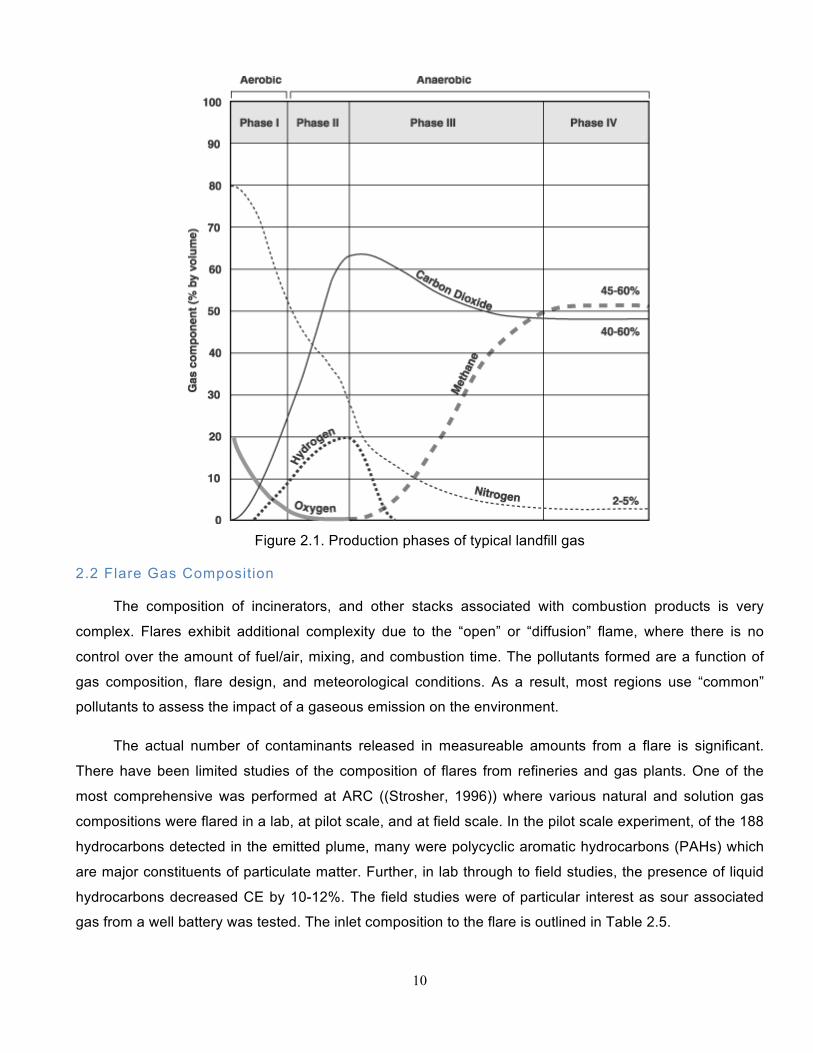
The composition is also a function of bacterial activity. The production phases of landfill gas can be
seen in Figure 1. In addition to waste composition and age of refuse, the presence of oxygen in the
landfill, moisture content and temperature affect the landfill gas composition.
10
Figure 2.1. Production phases of typical landfill gas
2.2 Flare Gas Composition
The composition of incinerators, and other stacks associated with combustion products is very
complex. Flares exhibit additional complexity due to the “open” or “diffusion” flame, where there is no
control over the amount of fuel/air, mixing, and combustion time. The pollutants formed are a function of
gas composition, flare design, and meteorological conditions. As a result, most regions use “common”
pollutants to assess the impact of a gaseous emission on the environment.
The actual number of contaminants released in measureable amounts from a flare is significant.
There have been limited studies of the composition of flares from refineries and gas plants. One of the
most comprehensive was performed at ARC ((Strosher, 1996)) where various natural and solution gas
compositions were flared in a lab, at pilot scale, and at field scale. In the pilot scale experiment, of the 188
hydrocarbons detected in the emitted plume, many were polycyclic aromatic hydrocarbons (PAHs) which
are major constituents of particulate matter. Further, in lab through to field studies, the presence of liquid
hydrocarbons decreased CE by 10-12%. The field studies were of particular interest as sour associated
gas from a well battery was tested. The inlet composition to the flare is outlined in Table 2.5.

11
Table 2.5. Sour Associated Gas Composition (Strosher, 1996)
Compound Mole %
Methane 45.4
Ethane 10.7
Propane 5.7
Butanes 2.4
Pentanes 2.6
Hydrogen Sulphide 22.8
There are significant gaps in the nature and emission rate of flared gas, however research is
ongoing. The uncertainty results in difficulty in predicting downwind concentrations of pollutants. This
uncertainty increases when coupled with the fact that most commercially available dispersion models are
designed for continuous sources (such as compressor stacks or incinerators) rather than intermittent
sources such as flares.

12
Chapter 3 CFD Modeling
3.1. Flare CFD modeling
Different mathematical models based on the numerical solution of the fluid dynamics equations have
been proposed for simulation and control of industrial combustion; however there is very little on flare
modelling. The advantage to CFD simulation over physical prototypes is the ability to simulate the actual
production platform rather than a smaller experimental model ((Ferguson, 2010)). Application of CFDs
reduces the cost of using actual flare experiments, although the results received by CFDs are only as
good as the input data. Further, inaccurate models lead to erroneous results. Castiñeira and Edgar,
2006a/b proposed the CFD tool Fluent for simulating two different types of flare. Three different
combustion flames of different sizes and compositions were simulated and demonstrated close agreement
between simulation and experimental data. The effect of crosswind on the combustion efficiency of the
flames is also simulated by CFD (Castiñeira and Edgar, 2008a; 2008b; Gottimukkala, 2008). The results
demonstrated that the high momentum flames are more sensitive to crosswinds whenever the jet velocity
increases. The effect of cross wind velocity and exit jet is also investigated using CFD (Fluent) by Lawal et
al., 2010. Results demonstrated that variation of these two parameters directly affect the flare efficiency.
Using CFD models we are able to evaluate different variables such as cross wind velocity, flare tip
diameter, heating value of the gas etc. on flare efficiency, temperature and gas composition profiles in the
flame. The drawback to the published studies above is the lack of detail in the kinetic model, there was no
study of emissions outside of carbon dioxide, and little detail on specifics such as pilot flame modelling
etc... In this work, we first develop the CFD model, validate with published data (using a more complex
kinetic model), and evaluate emissions outside of carbon dioxide. In our work a detailed reaction
mechanism (containing 23 species and 74 reactions) was used.
3.1.1. Governing Equations
CFD is based on solving conservation or transport equations for mass, momentum, energy, and
species. A set of partial differential equations consisting of six equations and six unknowns (density, three
components of velocity, temperature and pressure) which are all the function of three special dimensions
and time are given below:

13
3.1.1.1. Mass and species transport
Mass conservation can be expressed in terms of density or individual gaseous species (𝑌!), as
illustrated in equations 1 and 2 respectively.
!!!!+ ∇. 𝜌𝑢 = 𝑚!
.!!! (3.1)
!!!
𝜌𝑌! + ∇. 𝜌𝑌!𝑢 = ∇. 𝜌𝐷!∇𝑌! +𝑚!.!!! +𝑚!,!
.!!! (3.2)
In equation 1, 𝑚!.!!! is the production rate of the species by evaporating droplets or particles.
3.1.1.2. Momentum transport
!!!
𝜌𝑢 + ∇. 𝜌𝑢𝑢 + ∇𝑝 = 𝜌𝑔 + 𝑓! + ∇. 𝜏!" (3.3)
In equation 3, considering 𝑢 = [𝑢, 𝑣,𝑤]!, uu (dyadic tensor) is given by the tensor product of the
vectors 𝑢 and 𝑢! , the term 𝑓! is forces such as grad exerted from liquid droplets and 𝜏!" is stress tensor
defined as follows:
𝜏!" = 𝜇(2𝑆!" −!!𝛿!"(∇. 𝑢) (3.4)
In equation 4, 𝜇 is the dynamic viscosity of the fluid and 𝑆!" is the symmetric rate of strain tensor,
defined as follows:
𝑆!" =!!(!!!!!!
+ !!!!!!) 𝑖, 𝑗 = 1,2,3,… (3.5)
This equation can be computed by a Direct Numerical Solution (DNS), wherein the dissipative terms
are computed directly or Large Eddy Simulation (LES), wherein large scale eddies are computed directly
and sub-grid scale dissipative processes are modeled.
3.1.1.3. Energy transport
!!!
𝜌ℎ! + ∇. 𝜌ℎ!𝑢 = !"!"+ 𝑞.!!!𝑞!.!!! − ∇. 𝑞.!! + 𝜀 (3.6)
In this equation, the sensible enthalpy is the function of temperature, as follows:
ℎ! = 𝑌!! ℎ!,! and ℎ!,! 𝑇 = 𝐶!,!!!!
(𝑇!)𝑑𝑇! (3.7)

14
The term 𝑞.!!!in equation 6 is the heat release rate per unit volume from a chemical reaction, 𝑞!.!!! is
the energy transferred to the evaporating droplets, and 𝑞.!! is conductive and radiative heat fluxes,
calculated by equation 8, in which 𝑘 is the thermal conductivity.
𝑞.!! = −𝑘∇𝑇 − ℎ!,!! 𝜌𝐷!∇𝑌! + 𝑞.!! (3.8)
3.2. Flared studies: A case study
To investigate the total emissions from the flared gases, a CFD model using Fluent integrated with
detailed reaction mechanism has been developed. To validate a model, a case study of using an
experimental flare (lab scale size) burning methane has been adopted from the literature. Ideally a landfill
gas would be used as a case study. However, the published data regarding landfill flares do not include
parameters such as flow rate and stack specifications. We visited the Robin Hood Bay facility to collect
information on their flare operation. However, there was little data available. Further, the existing flare (a
simple candle stick flare) is scheduled to be replaced by a larger scale industrial type flare. (At this time
we will take the data from this flare and apply the methodology outlined below. Sentence unclear, which
flare? The experimental flare (lab scale size) referred to above?
3.2.1. Chemistry
There have been great advances lately in obtaining detailed reaction mechanism that can describe
hydrocarbon combustion in various temperatures and operating conditions (Mendiara et al., 2004).
However, using a complex mechanism with hundreds of compounds increases computational cost (days
to run models) with little gain in accuracy of predicting gas compositions and subsequent impact. A
reduced mechanism accomplishes the goal of predicting combustion efficiencies accurately and predicting
contaminants of concern in emissions. We first tested our CFD model with a very simple five global steps
mechanism to ensure the model was running properly. We were able to predict CO2 levels accurately,
however, this mechanism was limited in the breadth of species involved (Peters and Kee, 1987; Bilger et
al., 1990). We adopted the mechanism propped by Mendiara et al (2004) which has 23 species and 74
reactions.
3.2.2. Modeling parameters
We first needed to verify our CFD model and reaction mechanism. Castiñeira and Edgar studied a
lab scale methane flare in 2008. In this study the diameter of the stack at the middle of the domain is 7.2
mm. The fuel contained 15% methane. To simulate open combustion, a two dimensional domain (0.7*0.7
m2) is used for this simulation. The model is defined and meshed in Gambit. Gambit is one of the well-

15
known and user-friendly preprocessor ((ANSYS, 2012) not in Refs) to create the geometry and meshing
for importing to Fluent. (The overall 129,560 cells with the similar size considered in the domain. Sentence
unclear). The primary temperature of the exit gas is considered at 2000 K. The temperature provides the
ignition energy for the gases at the beginning. As most of the reactions in this mechanism are exothermic,
the required extra heat for all the reactions in the flame will be supplied by the heat which is released from
these reactions.
To model the combustion process with Fluent, the segregated, steady state solver is used for
computations. The standard K-ε model that includes two extra transport equations to represent the
turbulent properties of the flow is used without any change in default constant values of Cε1 and Cε2.
The in situ adaptive tabulation (ISAT) method was used to save computational work that is a most
powerful tool to accelerate detailed stiff chemistry. A speedup of two to three orders of magnitude (is
assisted assists) a simulation that would take months without considering ISAT to be run in days instead
((Fluent, 2012)). The absolute and relative error tolerances were set as 1*10−6 and 1*10−9 , respectively.
These values were previously used by Castiñeira, 2008 for a similar study. The ISAT error tolerance was
set as 1*10 −4. The maximum storage capacity was set as 200 Mb. The reference time step was set as
0.001.
3.3. Results and discussion
After modeling the flare gas combustion by application of a methodology discussed in the previous
sections, the results of CH4 combustion and CO2 production from the flared gases were compared with
the experimental results. Figure 3.1. compares the experimental and simulation results of methane
combustion in the middle axes of the flare. Both the data and the model show the same trend but at
different distances in the flame. This is due to the fact that in the experiment the combustion process
starts at some distance from the flare tip. However, in the simulated flare, as the gas and the air are
exiting simultaneously from the flare tip with a high temperature, methane combustion occurs immediately
after releasing from the tip. The critical aspect is that we were able to predict final product emissions,
combustion efficiency, and temperature of the flame.

16
Figure 3.1. Experimental and simulation mass fraction of CH4
The results of CO2 mass fraction can be seen in Figure 3.2. The minimum mass fraction of CO2 is 0.11
which is in agreement with the experimental results. However, the maximum in the simulation is achieved
at a shorter distance from the flare tip. Again, this is a result of the reason stated above. Again the model
matched both trend and concentrations in flame.
Figure 3.2. Experimental and simulation mass fraction of CO2
After comparing the results of the methane combustion and CO2 production from the simulation with
experimental data, the concentration of other species existed in the considered reaction mechanism were
also analyzed. We demonstrate this with the other major carbon species, carbon monoxide (CO), an
important gas due to its toxicity and GHG effect. (Figure 3.3). The CO shows a peak early in the flame
where we would expect the largest level of incomplete combustion products. There is no experimental
data because the study did not consider other compounds. This demonstrates the use of the CFD model,
0
0.02
0.04
0.06
0.08
0.1
0.12
0.14
0.16
0.18
0 5 10 15 20 25 30 35 40 45 50 55 60 65
XC
H4
X/d
Experimental
Simula8on
0
0.02
0.04
0.06
0.08
0.1
0.12
0 10 20 30 40 50 60
XC
O2
X/d
Experimental
Simulation

17
with the ability to predict compounds not measured due to lack of analytical or capture equipment on the
flare.
Figure 3.3. Simulation mass fraction of CO
As the experimental data from Castiñeira and Edgar (2008a) was in a controlled lab setting, the
flare is able to achieve high combustion efficiencies. However, as (Strosher (1996)) demonstrated, as one
moves from a lab scale to pilot to field, and gas composition changes from pure methane to mixtures, the
combustion efficiency drops. This is largely due to poor mixing between air and feed gas, where the air
surrounds the flare rather than co-flowing with the fuel (as in the lab). The CFD model was adapted to
account for this by tuning the air: fuel ratios to match emission of carbon dioxide. This is an example of
how in an industrial flare, the CFD model must be combined with some basic emission data (this data is
typically available as companies are to measure key components of the flare emissions). The CFD model
can provide additional information about the nature of the emissions that would be extremely costly and
technically difficult to obtain. Further, the model can determine combustion efficiency, effect of varying
flow rates, stack height and diameter, and wind speed on emissions. We are continuing this work by using
the developed model to predict actual landfill/industrial flares. Contaminants of concern in the gas emitted
can be predicted as above and used to determine the impact of the flare on the surrounding area. From
this type of analysis we can determine combustion efficiency, effect of varying flow rates, stack height and
diameter, and wind speed on emissions. We are continuing this work by using the developed model to
predict actual landfill/industrial flares. Our next step is to incorporate the mechanism outlined in Appendix
2 (with sulfur compounds) to predict emissions from flare gases containing H2S.
0
0.05
0.1
0.15
0.2
0.25
0 5 10 15 20 25 30
XC
O
X/d
18
Chapter 4 Environmental Risk Assessment
4.1. Environmental risk assessment
Environmental risk analysis is a systematic process of assessing, managing and communicating risk
to human health caused by an event or activity occurring in the environment. Risk analysis is a detailed
examination that consists of risk assessment, risk evaluation and risk management alternatives that are
produced to recognize the nature of unwanted, adverse consequences to human life, health, property and
environment (Bondad et al., 2008). The Food and Drug Administration ((FDA, 2002) not in Refs) defines
“risk analysis as a tool to enhance the scientific basis of regulatory decisions.” It includes risk assessment,
risk management and risk communication activities. Each component has unique responsibilities. Risk
assessment provides information on the extent and characteristics of the risk attributed to a hazard. Risk
management includes the activities undertaken to control the hazard. Risk communication involves an
exchange of information and opinion concerning risk and risk related factors between the risk assessors,
risk managers and other interested parties (Fjeld et al. 2006). In simple terms:
Risk analysis = risk assessment + risk management + risk communication
These three components of risk analysis are dependent on one another for analyzing the magnitude
of risk caused by the release of the contaminants, as can be seen in Figure 4.1. Environmental risk
assessment is the characterization of adverse health effects that results from human and ecological
exposures to environmental hazards. The field of environmental risk assessment has grown in the last two
decades due to the increase in public concern about the adverse effect of chemicals and hazards to the
wildlife and ecosystem. Environmental risk assessment uses a set of tools to identify the likelihood and
magnitude of adverse effects posed by environmental agents on human health and to natural resources.
Conclusively, risk assessment is a systematic process for describing and quantifying the risk related to
hazardous substances, processes, actions, or events (Covello et al., 1993).

19
Figure 4.1. Different components of risk analysis (Brunk, 1998)
However, most environmental risk assessments are performed to answer a question or resolve an
issue, such as: Is it safe for a proposed chemical plant to operate in this location or is it safe to dispose?
Risk Assessment
ü Hazard (vs. “risk”) identification
ü Hazard characterization ü Exposure assessment ü Risk estimation
Risk communication
Receiving messages from risk Stakeholders
ü Perceptions of risk magnitude ü Prioritization of risk ü Perception of risk acceptability
Delivering messages to risk Stakeholders
ü Best estimate of risk ü Standards of safety ü Management strategies chosen
Risk Management
Risk evaluation
ü Profile the risk ü Rank Risks ü Set of risk assessment policy ü Communication risk assessment
Risk management option assessment
ü Identify management options ü Select safety standard ü Final management design
Monitor & review effectiveness
Implement management strategy

20
The Canadian Council of Ministers of the Environment (CCME) (1996/2007) has set forth guidelines for a
three-tiered system that may be used to derive environmental quality criteria. The following components
outlined by CCME are involved in the risk assessment process (CCME, 1996/2007):
Figure 4.2. Different components of risk assessment process (CCME, 1997)
As per Figure 4.2, the receptor is the person or population exposed to the contaminant at the
exposure point. One of the important factors in determining exposure includes the characteristics of
receptors. For most of the equations used to estimate the exposure, at least two terms (e.g. age, body
weight and gender), attempt to define a specific receptor’s characteristics or parameters. Some
characteristics like body weight, volume of air inhaled per unit, amount of soil consumed inadvertently and
time spent indoors and outdoors for human and ecological entities should be evaluated as a part of the
environmental risk assessment process. The values for each of the receptors vary significantly and, for
this reason, which receptors receive the greatest exposure from the contaminant needs to be defined.
Hazard, a measure of harm or the potential of the event to cause harm, is one of the components of
the risk assessment process. Different types of hazards exist. Some are natural, while industrial or
technological hazards are caused by human beings.
Exposure is one of the components of the analysis phase of a risk assessment. It is a measure of the
amount that the likely recipient of a specific hazard absorbs. For any special hazard, the greater the
exposure, the greater the risk of an adverse effect is on health. Exposure can be simply identified as the
amount of the agent that is available to a human or animal. Exposure can occur through different
pathways for humans, as illustrated in Figure 4.3. The absorption of chemicals is related to the route of
exposure. Furthermore, the absorption of a chemical also is affected by its chemical and physical
properties. In simple terms, chemicals that are soluble in fat can be absorbed more easily into the body.

21
These risk assessment processes are divided into different components according to different
organizations such as Environmental Protection Agency (EPA) and CCME.
The EPA baseline risk assessment process includes data collection and evaluation, exposure
assessment, toxicity assessment and risk characterization (USEPA, 1999), as can be seen in Figure 4.4.
Figure 4.3. Major pathways of human exposure to environmental contaminants (Health Canada,
1995)
There are many different risk assessment approaches proposed by regulations agencies such as
EPA and CCME. Most of these approaches are comprised of four steps, which are outlined below:
ü Hazard identification and assessment
ü Exposure assessment
ü Dose-Response assessment
ü Risk characterization
These four steps provide a better understanding of a system’s environmental risk assessment. Thus,
these steps are described in the following sections.

22
Data collection and
evaluation
ü Gather and analyze
relevant site data
ü Identify potential
chemical of concern
Exposure assessment
ü Analyze contaminant
releases
ü Identify exposed
populations
ü Identify potential
exposure pathways
ü Estimate exposure
concentrations
pathways
ü Estimate contaminant
intakes for pathways
Toxicity assessment
ü Collect qualitative and
quantitative toxicity
information
ü Determine appropriate
toxicity values
Risk characterization
ü Characterize potential
for adverse health
effects to occur
ü Evaluate uncertainty
ü Summarize risk
information
Figure 4.4. Different processes of risk assessment according to EPA (USEPA, 1999)

23
4.1.1. Hazard identification and assessment
The potential for chemicals to cause adverse effects on the lives of humans, plants and animals can
be provided and understood by considering hazard assessment. Hazard identification is the first stage in
hazard assessment (Phua et al., 2007). It includes gathering and evaluating toxicity data on the types of
health impact or disease that may be produced by a chemical and the conditions under which the impact
or the disease is produced. In order to identify the hazard, the data for all contaminants at a site should be
examined and the data to stress the chemicals of concern should be consolidated. The following steps
show the data needed in hazard identification stages (Khan, 2008):
• Site history
• Land use
• Contaminant levels in media
ü Air
ü Ground water
ü Surface water
ü Soils and sediments
• Environmental characteristics affecting chemical fate and transport
ü Geologic
ü Hydrologic
ü Atmospheric
ü Topographic
• Potentially affected population
• Potentially affected biota
Hazard assessment is most commonly used for analyzing the effects of chemicals on the natural
environment. The definition of hazard is formulated by Klopffer (1994) as follows:
Hazard = Exposure * Effect (4.1)
This shows that there is no hazard (bad effect) if there is no exposure. The following steps are
involved in hazard assessment:
1) The contaminant data should be sorted by medium (e.g. ground water, soil, etc.) for both
carcinogens and non-carcinogens.
2) The average and range of each chemical concentration observed at the site should be
demonstrated.

24
3) The toxicity scores (TS) for each chemical in each medium due to carcinogens and non-
carcinogens should be demonstrated as follows:
For non-carcinogens: Considering exposure duration, the toxicity score is estimated as follows:
TS = RFCCMax (4.2)
RFC = Chronic reference concentration (an estimate of acceptable daily intake)
For carcinogens: TS = SF * CMax (4.3)
SF = Slope factor (slope factor here is considered for daily intake
(slope factor * day))
4) Ranking the compounds by toxicity scores for each exposure route
5) For each exposure route, selecting those chemicals that compose 99 percent of the total score.
4.1.2. Exposure assessment
There has been a significant increase in awareness of environmental issues in recent years and there
is a great concern among the people over how their health is affected by environmental factors. Exposure
assessment includes estimating the dose or concentration of the contaminant taken in by human and
ecological receptors per unit of time. Characterization of the exposure setting, identification of exposure
pathways and quantification of exposure are different steps in exposure assessment.
Using the exposure assessment, the following questions can be answered:
1) Who and what is exposed (e.g. people, aquatic ecosystems)?
2) How much exposure occurs?
3) How often and how long does the exposure occur and what is its frequency and duration?
Various plausible exposure pathways exist for every valued ecosystem component. Different
pathways include direct contact, water ingestion, soil or sediment ingestion, and through the food chains.
Indirect contact should be considered as well.
Using the fate and transport model, which is validated through field measurement, the information for
input into an exposure model can be provided. Different steps for calculating exposures to chemicals
present in the environment can be seen in Figure 4.5.
For calculating people’s and ecological entities’ expose to environmental contaminants, several
assumptions need to be considered.

25
The average values are generally used for:
• Body weight
• Amount of food and water consumed
• Amount of air breathed, and
• Number of times people and ecological entities are exposed to contaminants over their lifetime
The exposure pathway describes how the contaminants go into the environment from their source to
humans or other living organisms.
Exposure pathways include the following steps:
• Source of contamination
• Environmental media
• Point of exposure
• Receptor person or population; and
• Route of exposure
It is noteworthy that the source of environmental contaminants varies from place to place. It can
consist of exhaust from cars, wastewater released by factories and mills, waste disposal sites or closed
factories or disposal sites. Furthermore, a number of natural sources can release various substances into
the environment.
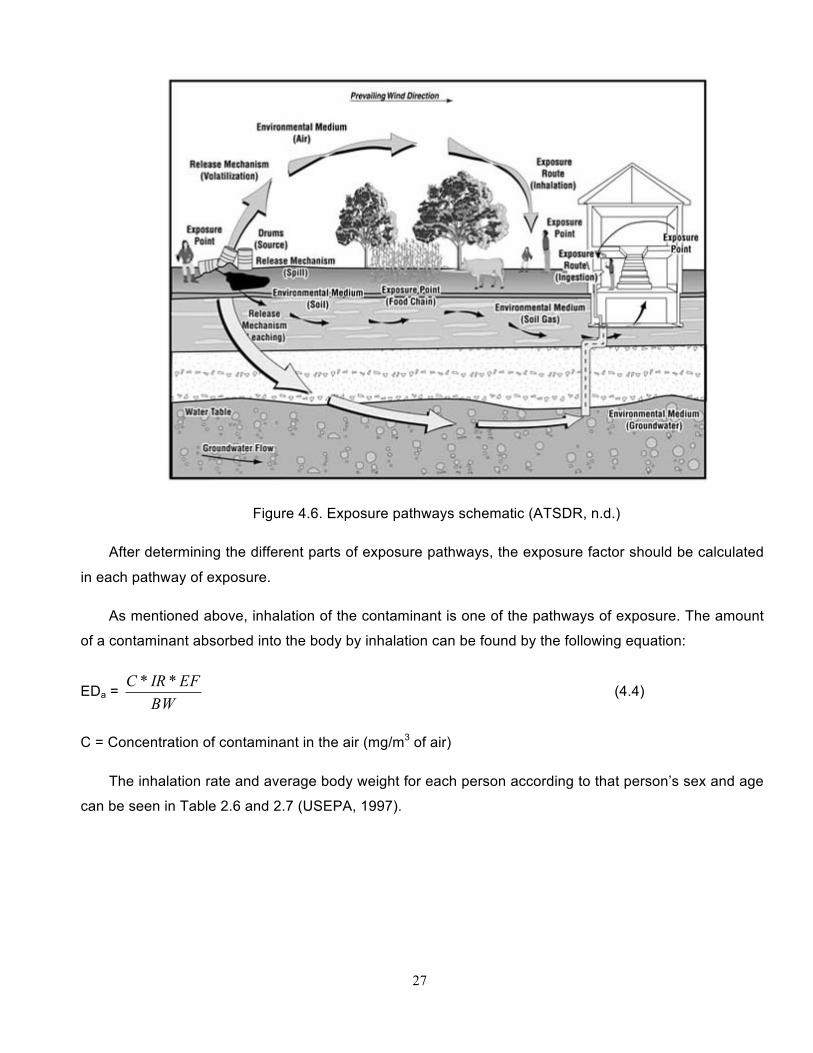
When the contaminants are released from their sources, they can travel over different environmental
media to reach the points where human exposures can occur. For humans, the major environmental
media are water, air, food and soil. Figure 4.6 demonstrates how contaminants are transported through
the food chain and affect human health through exposure and food intake.

26
Figure 4.5. Different steps for calculating exposure to chemicals (Health Canada, 1995)
The point of exposure is where contact with the contaminants occurs. Different locations that people
are exposed during the day and night (e.g. homes, workplaces, lakes, rivers or other bodies of water) can
be the point of exposure.
The individual or population that is exposed to the contaminant at the point of exposure is the
receptor. For example, people may be exposed to the contaminated air by going outside and breathing.
Finally, the route of exposure is the way that the contaminant enters into the human and animal body.
Ingestion, inhalation and skin contact are three general routes by which human and animals take the
contaminant into their body.
27
Figure 4.6. Exposure pathways schematic (ATSDR, n.d.)
After determining the different parts of exposure pathways, the exposure factor should be calculated
in each pathway of exposure.
As mentioned above, inhalation of the contaminant is one of the pathways of exposure. The amount
of a contaminant absorbed into the body by inhalation can be found by the following equation:
EDa = BW
EFIRC ** (4.4)
C = Concentration of contaminant in the air (mg/m3 of air)
The inhalation rate and average body weight for each person according to that person’s sex and age
can be seen in Table 2.6 and 2.7 (USEPA, 1997).

28
Table 4.1. Average body weight for each age group according to their sex (USEPA, 1997)
Model Age Group Body Weight (kg)
Male Female
0-17 34.3 33.0
18-44 78.2 64.3
45-64 79.9 68.0
65+ 74.8 66.6
Table 4.2. EPA recommended inhalation values (USEPA, 1997)
Age Group (years) Sex Inhalation values
(m3/day)
<1 Both 4.5
1-2 Both 6.8
3-5 Both 8.3
6-8 Both 10
9-11 Male 14
Female 13
12-14 Male 15
Female 12
15-18 Male 17
Female 12
19-65+ Male 11.3
Female 15.2
Moreover, the amount of a contaminant taken into the body per food is calculated for each individual
food by the following equation:

29
(Food group 1) (Food group 2)
EDf = BW
EFCRCF ** + BW
EFCRCF ** (4.5)
4.1.3. Dose-Response assessment
Dose-Response assessment is the step of the risk assessment process that connects the likelihood
and severity of damage on human health from exposures to different levels of risk agents. The
quantitative relationship between the level of exposure and the intensity of the resulting adverse health
effects is represented by graphs. This graph, which can be seen in Figure 2.14, shows the cumulative
exposure or rate of exposure per unit of time.
Figure 4.7. Dose-Response curve (USEPA, 1991)
The extrapolation of dose relationships from a specific population to another group or from animal
studies to human beings should be conducted according to the following factors:
ü Difference in physical dimensions like body weights
ü Difference in intake
ü Different life span
ü Difference in the absorption rate of chemical, nature, routes.
Regression methods can be used for finding the dose and response relationship if enough data are
available. Dose-Response models can be divided into three main categories. These categories are
described in the following paragraphs.
Simple Dose-Response models: These models show the single measurement of dose (e.g.
cumulative exposure) to a single measure health response (e.g. number of fatalities). These models are
used to estimate the number of cases of cancer caused by exposure to low level radiation. For
applications of this model, dose-response relationships are usually shown by curves with thresholds.

30
Tolerance distribution models: These models are based on the fact that each person in the population
has an individual threshold tolerance associated with the specific risk agent. In these models, it is
assumed that the probability that a particular individual will experience an adverse effect when exposed at
the dose level d is the same as the probability for the tolerance level of the individual less than d. The log-
probit model is the most commonly used tolerance models. It is popular because the result of toxicity tests
often fit the shape assumed in the model. This model is usually used for determining the dose-response of
the exposure to toxic gases and estimation of infections from disease caused by organisms.
Mechanistic models: These models usually show the biological processes that lead to an adverse
effect as a series of events evolving over time. Although such models can become mathematically
complex, they are usually based on very simple biological assumptions. Hit, multistage, and cellular
proliferation models are the most well-known in this case (Fjeld, 2006). Mathematical equations of
different dose-response models can be seen in Table 2.8.
Table 4.3. Mathematical equations of several dose-response models used in cancer risk assessment (Edler et al., 1998)
Model
Equations for the probability of
response (Proportion of population
affected at dose d)
Parameter constraints
Probit F(d) = φ (a+b lnd) b>0
Logit F(d) = [1-exp(-(a+b lnd))]-1 b>0
Weibull F(d) = 1 – exp(-bdk) b>0, K>0
One hit P(d) = [1-exp(-bd)] b>0
Multistage F(d) = [1-exp(-∑=
k
i
ii da
0
)] ai≥ 0
The standard procedure for assessing non-cancer risks related to hazardous components uses a No
Observed Adverse Effect Level (NOAEL) approach. NOAEL is the point in which no-effect level is
observed. By applying an uncertainty factor to this point, it may be then used to estimate a dose limit for
humans. This limit is below a presumed threshold and shows the acceptable exposure level. For
establishing a permissible exposure levels for humans for non-carcinogens, the NOAEL is used for finding
the RFD (Reference Dose) as follows:

31
RFD = UF
NOAEL (4.6)
UF is the uncertainty factor, which is assumed to be 10 when relevant research based information is
missing.
In a new dose-response procedure, the benchmark dose method is used instead of NOAEL. In
benchmark modeling, the bench mark (BM), which is the dose related to 10% response, is evaluated. The
lower bond of 95% confidence interval for this BM is called LBM (Faustman, 1996).
To determine the best model that can fit the dose and response data, EPA develops the Benchmark
Dose Software (BMDS) to facilitate the application of benchmark dose (BMD) methods to the EPA
hazardous pollutant risk assessment. This software helps find the Bench Mark (BM) and Lower Bond of
95% of confidence interval (LBM) associated with different doses and responses. After finding BM and
LBM, the RFD is calculated as follows:
RFD = UFLBMBM ,
(4.7)
A different approach is used for carcinogens which are generally assumed to have a non-threshold
dose-response. A decision about these chemicals (carcinogens) must be made to determine “how large a
risk of cancer can be accepted, in order to set acceptable intake levels” (Health Canada, 1995). Different
acceptable levels of risk are used around the world. These levels vary between one extra cancer death
per ten thousand people and one extra cancer death per million people exposed to the contaminants over
their entire lifetime.
After establishing the acceptable level of risk, a dose that people can be exposed to on a daily basis
over their entire lifetime that will not exceed the accepted level of risk of cancer can be calculated. As the
acceptable dose is directly related to the decision about an acceptable level of risk, it is called Risk-
specific Dose (RsD). Considering each carcinogen, which has its own slope factor, the RsD is calculated
as follows (Health Canada, 1995):
RsD = Acceptable level of risk / Slope factor (4.8)
4.1.4. Risk characterization
By integrating exposure assessment and toxicity assessment, which are discussed earlier, the
probability of negative effects is understood. Risk characterization is carried out for individual chemicals
and then summed for a mixture of chemicals (Considering that additivity is assumed). Next, the amount of

32
these chemicals can be compared with different guidelines on chemicals concentration. These guidelines
suggest different criteria by considering different chemicals and ways of exposure.
Qualitative and quotient methods are suitable for risk characterization. The judgment will be relied on
using qualitative methods, such as a ranking system that shows the level of risk in terms of high, moderate
or low. If there is sufficient information available about the Expected Environmental Concentration (EEC)
in the most important medium or media and where there are adequate studies available in the literature to
determine the toxicological benchmark, the quotient method may be used. The quotient is calculated by
“taking the ratio of the EEC and a BC (Benchmark Concentration) (CCME, 1996)”. If the quotient is less
than 1, it shows that the risk is slight and little or no action is required. If the quotient is near 1, it shows
uncertainty in the risk estimate and additional data is required. Finally, if the quotient is more than 1, it
shows that the risk is greater and regulatory action may be indicated (CCME, 1996).
4.2. A developed risk-based methodology
A risk-based methodology based on the EPA framework integrated with the flare CFD modeling was
developed to assess the effect of the flare gas emissions on human health downstream of the flare. The
developed methodology can be found in Figure 4.9. Emissions predicted from the CFD model are passed
to a stack dispersion model, which predicts species concentrations downstream of the flare (as a function
of distance from flare). For concentrations at different distances, the hazard quotient method can be used
to determine the effects of the flared gases. After adopting the species concentrations of the flared gases,
and modeling the transport of contaminants at the downstream of the flare, the hazard quotient method
can be used to consider the effects of the flared gases on human health.
By integrating exposure and toxicity assessment, the probability of negative effects is determined. Risk is
calculated for individual chemicals and then summed for a mixture of chemicals (considering additive
property of risk). The HQ is calculated by taking the ratio of exposure chemical concentration and TLV-
TWA for each chemical of concern, as represented by Equation 4.9 (Abbassi et al., 2011).
𝐻𝑄 = !"#$%&'( !"#!$#%&'%("# !"#!!"#
= !"#$%#&'(&)"#∗!"#$ !"#$%/!"!"#!!"#/!"
(4.9)
HQ is used to determine the distance from the flare which is safe for human exposure. Wherever the HQ
is less than one, it demonstrates the inhaled species concentrations are less than the human tolerance
level and there is no effect on the human health.

33
Figure 4.10. Risk-based methodology for evaluating a flare performance
4.3. A risk-based methodology: A case study
A risk-based methodology developed in section 4.2. has been applied to the case of the Kangiran flare.
Although this case study is from oil and gas facilities, it has been adopted as it can provide us with the
required information to illustrate the developed process. By having the required information of a landfill
gas flare and surrounding environmental conditions, the same process developed in section 4.2 can be
applied for managing the performance of a specific landfill flare.
Identifying the landfill flared gases
Modeling the stack using CFD pre-‐processors
The concentrations and the flow rate of the gases should be determined
The stack diameter should be known The mesh size should be selected by using
sensitivity analysis
Applying the CFD to model the flaring process
Fluent is the CFD software used in this paper
Finding the chemical species after flaring The species with maximum concentrations selected as the chemicals of concern
Application of dispersion model to determine the surrounded concentrations
Aermod is an EPA dispersion model
Dose-‐Response assessment for the chemicals of concern
Risk criteria for different contaminants can be adopted from EPA and CCME
Risk characterization to determine the safe surrounding environment
HQ method is used in this paper to characterize the risk

34
4.3.1. Specification of a considered site
The Shahid Hashemi-Nejad (Khangiran) natural gas process facility is one of the most important gas
processing facilities, located in northeastern Iran in an open inhabitable range land, semi arid and dusty
with windblown sand. The feed gas is supplied from the Mozdouran gas fields. This gas process facility
consists of 5 sour gas treating unit, 3 dehydration units, 3 sulfur recovery units, 2 distillation units, 2
stabilizer units and 14 additional units related to other services. The wind direction in the Khangiran
vicinity is from northwest to southeast. This condition occurs in the Khangiran gas process facility for 90%
of the year. For the remainder of the year, the wind direction changes, and the wind blows from southeast
to northwest. Wind roses were used to give a succinct view of how wind speed and direction are typically
distributed and to determine the direction of the prevailing wind in the vicinity of Khangiran. During 10% of
the year, the wind direction is 160 degrees, which causes the wind to carry toxic gases to the personnel
dormitory. This dormitory is located 1050 meters away from the flare stack and it is 200 meters in length.
The release time was considered to be 1 h.
4.3.2. Risk Analysis
SO2 is the toxic gas considered during the release time (1 h) in this study. SO2 is a colorless gas
which smells like burnt matches. It can be oxidized to sulfur trioxide, which in the presence of water vapor
is readily transformed to sulfuric acid mist. SO2 with acute exposure of 5 ppm may cause dryness of nose
and throat and a miserable increase in resistance to bronchial air flow. SO2 increasing up to 6 to 8 ppm
causes a decrease in tidal respiration volume. Sneezing, cough & eye irritation occur at 10 ppm. SO2
concentration of 20 ppm may cause Bronchospasm and 50 ppm causes extreme discomfort, but no injury
in less than a 30 minute exposure. Finally, inhalation of 1000 ppm more than 10 minutes causes death
(Thienes and Haley, 1972). The Concentration of SO2 in this modeling scenario is 100.63 kmole/hr.
The dispersion of SO2 in the studied area has been estimated by using AERMOD. The results of this
modeling are summarized in Table 4.4. demonstrated that personnel dormitory is covered by a plume
with a concentration of more than 5 ppm of SO2 released from the flared gases.
Table 4.4. Concentrations of SO2 in two different areas considered in this modeling scenario
Area SO2 Concentration (ppm) Number of Employees
1 2 200
2 5 220
35
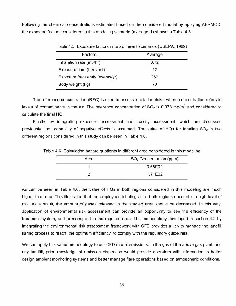
Following the chemical concentrations estimated based on the considered model by applying AERMOD,
the exposure factors considered in this modeling scenario (average) is shown in Table 4.5.
Table 4.5. Exposure factors in two different scenarios (USEPA, 1989)
Factors Average
Inhalation rate (m3/hr) 0.72
Exposure time (hr/event) 12
Exposure frequently (events/yr) 269
Body weight (kg) 70
The reference concentration (RFC) is used to assess inhalation risks, where concentration refers to
levels of contaminants in the air. The reference concentration of SO2 is 0.078 mg/m3 and considered to
calculate the final HQ.
Finally, by integrating exposure assessment and toxicity assessment, which are discussed
previously, the probability of negative effects is assumed. The value of HQs for inhaling SO2 in two
different regions considered in this study can be seen in Table 4.6.
Table 4.6. Calculating hazard quotients in different area considered in this modeling
Area SO2 Concentration (ppm)
1 0.68E02
2 1.71E02
As can be seen in Table 4.6, the value of HQs in both regions considered in this modeling are much
higher than one. This illustrated that the employees inhaling air in both regions encounter a high level of
risk. As a result, the amount of gases released in the studied area should be decreased. In this way,
application of environmental risk assessment can provide an opportunity to see the efficiency of the
treatment system, and to manage it in the required area. The methodology developed in section 4.2 by
integrating the environmental risk assessment framework with CFD provides a key to manage the landfill
flaring process to reach the optimum efficiency to comply with the regulatory guidelines.
We can apply this same methodology to our CFD model emissions. In the gas of the above gas plant, and
any landfill, prior knowledge of emission dispersion would provide operators with information to better
design ambient monitoring systems and better manage flare operations based on atmospheric conditions.

36
Chapter 5 Conclusion
5.1. Conclusion
In this work we have developed a CFD model for use as a tool in landfill gas flaring. The costs
associated with large scale testing of landfill flares and improper operation due to lack of predictive models
could be reduced using the CFD model. We validated the model with published data and developed a
method to scale up our model to accommodate the non-ideal mixing encountered in landfill flares. Finally
we proposed methodology to integrate the CFD model with dispersion and risk models to evaluate
environmental impact and which can be used as a tool in designing environmental monitoring networks.
As the report indicates, the model is general but the input parameters will be a function of the specific
landfill as the composition of the landfill gas is a function of waste, landfill age and season. The chemical
reaction mechanism used must balance computational time and cost with emission predictions that reflect
contaminants of concern and flame temperature (or combustion efficiency). By integrating the CFD and
environmental risk assessment, we have a tool to manage the flaring which incorporates human and
environmental health concerns.
5.2. Recommendations
Based on the investigations of the landfill gas flare composition and modeling of the flaring process
using CFD, the authors are (contusing?) continuing the work:
1. Collection of data from local landfill flares and incinerators for input to our CFD model for a real case
study
2. Modeling different processes such as steam injection and air injection, processes used to increase the
efficiency of landfill gas flaring and validation of the results with real cases
3. Application of a methodology developed in this research to a landfill gas flare to create a field case
study which identifies the carcinogenic and non-carcinogenic risks of flared gases.
Acknowledgements
The authors gratefully acknowledge the financial support provided by the Harris Centre of Memorial
University under the Waste Management Applied Research Fund of 2010-2011.

37
References:
Abbassi, R., Dadashzadeh, M., Khan, F. and Hawboldt, K. 2011. Risk-based prioritisation of indoor air pollution monitoring using computational fluid dynamics. Indoor and Build Environment, DOI: 10.1177/1420326X11428164 Agency for Toxic Substances and Disease Registry (ATSDR): http://www.atsdr.cdc.gov/ Alian, D. 1997. Landfill gas management in Canada. Proceedings of air and waste management
association’s annual meeting and exhibition, Quebec, Canada.
Anonymous. 2010. Waste management opens first-ever private landfill gas to energy in south western
Ontario. ON, Canada.
Bilger, R.W., Starner, S.H., Kee, R.J. 1990. On reduced mechanisms for methane-air combustion in non-
premixed flames. Combustion and Flame, 80: 135-149.
Bondad, MGR., Arthur, J.R. and Subasinghe, R.P. 2008. Understanding and applying risk analysis in
aquaculture. Rome, Italy: Food and Agriculture Organization of the United Nations.
Brosseau, J., Heitz, M., 1994. Trace gas compounds from municipal landfill sanitary sites. Atmos. Environ.
28 (2), 285–293.
Brunk, C. 1998. Risk management workshop.
http://cmte.parl.gc.ca/Content/HOC/committee/362/envi/reports/rp1031697/envi01/15-ch8-e.html
Castiñeira, D., A. 2006a. Computational fluid dynamics simulation model for flare analysis and control.
PhD thesis, Austin, Texas: The University of Texas at Austin.,.
Castiñeira, D., and Edgar, T.F. 2006b. CFD for simulation of steam-assisted and air-assisted flare
combustion systems. Energy and Fuels, 20(3): 1044-1056.
Castiñeira, D., and Edgar, T.F. 2008a. CFD for simulation of crosswind on the efficiency of high
momentum jet turbulent combustion flames. Journal of Environmental Engineering, 134(7): 561-571.
Castiñeira, D., and Edgar, T.F. 2008b. Computational fluid dynamics for simulation of wind-tunnel
experiments on flare combustion systems. Energy and Fuels, 22(3): 1698-1706.
Canadian Council of Ministers of the Environment (CCME). 1996. A framework of ecological risk
assessment: General guidance. The national contaminated sites remediation program, Winnipeg,
Manitoba, Canada.
Canadian Council of Ministers of the Environment (CCME). 2007. Canadian water quality guidelines for
the protection of aquatic life.
Covello, V.T., and Merkhofer, M.W. 1993. Risk assessment methods, approaches for assessing health
and environmental risks. New York and London: Plenum Press, ISBN: 0-306-44382-1.
Dincer, Faruk; Odabasi, Mustafa; Muezzinoglu, Aysen. Journal of Chromatography A vol. 1122 issue 1-2
July 28, 2006. p. 222-229

38
Edler, L., and Kopp-Schneider, A. 1998. Statistical models for low dose exposure. Mutation Research,
405: 227-236.
Eklund, B., Anderson, E.P., Walker, B.L. and Burrows, D.B. 1998. Characterization of landfill gas
composition at the fresh kills municipal solid waste landfill. Environmental Science and Technology, 32:
2233-2237.
Environment Agency. 2002. Investigation of the composition, emissions and effects of trace components
in landfill gas. R&D Project, P1-438.
Faustman, M.E. 1996. Review of Noncancer Risk assessment: Application of Benchmark Dose Methods.
Department of environmental health, Seattle, WA: University of Washington.
Ferguson S. 2010. CD-adapco, http://www.kr.cd-adapco.com/press_events/Dynamics/27/flare.html#
Fjeld, R.A., Eisenberg, N.A, and Compton, K.L. 2006. Quantitative environmental risk analysis for human
health. N.Y.: John Wiley & Sons, ISBN-13: 978-0-471-72243-4.
Fluent. 2012. User manuals 6.2. Fluent Inc.
Gottimukkala, B.C.V. 2008. CFD simulation of industrial flares with reduced mechanism and NOx
dispersion from vehicular exhaust pipe. M.Sc. Thesis, Lamar University, Texas, USA.
Health Canada. 1995. Investigating human exposure to contaminants in the environment : A community
handbook. Ottawa: Minister of National Health and Welfare, ISBN: 0-662-23543-6.
Karapidakis, E.S. and Tsava, A. 2010. Electric power production by biogas generation at Volos landfill in
Greece. Department of natural resources and environment, Greece.
Khan, F.I. 2008. Risk assessment: Class handout. Memorial University of Newfoundland, St. John’s, NL,
Canada.
Kim, K.H., 2006. Emissions of reduced sulfur compounds (RSC) as a landfill gas (LFG): a comparative
study of young and old landfill facilities. Atmospheric Environment 40: 6567–6578.
Klopffer, W. 1994. Environmental hazard Assessment of chemicals and products Part II: Persistence and
degradability of organic chemicals. Environmental science and pollution research, 1(2): 108–116.
Lawal, S., Fairweather, M., Ingham, D., Ma, L., Pourkashanian, M. and Williams, A. 2010. Computational
study of combustion in flares: structure and emission of a jet flame in turbulent cross-flow. GERG
Academic Network Event, Brussels.
Mendiara, T. Alzueta, M.U. Millera, and Bilbao R., 2004, An Augmented Reduced Mechanism for Methane
Combustion, Energy and Fuels 18(3).
Peters, N. and Kee, R.J. 1987. The Computation of stretched laminar methane-air diffusion flames
using a reduced four-step mechanism. Combustion and Flame, 68(1): 17-29.
Phua, S.T.G., Davey, K.R., Daughtry, B.J. 2007. A new risk framework for predicting chemical
residue(s)—Preliminary research for PCBs and PCDD/Fs in farmed Australian Southern Bluefin Tuna
(Thunnus maccoyii). Chemical engineering and processing, 46(5): 491-496.

39
Strosher, M. 1996. Investigations of flare gas emissions in Alberta. Final report to Environment Canada,
Alberta Energy Utilities Board and the Canadian Association of Petroleum Producers, Calgary, Alberta,
Canada.
Thienes, C., and Haley, T.J. 1972. Clinical Toxicology, 5th ed., Philadelphia:Lea and Febiger, , p. 198.
U.S. Environmental Protection Agency (USEPA). 1989. Exposure factors handbook, EPA/600/8-89/043.
U.S. Environmental Protection Agency (USEPA). 1991. Risk Assessment for Toxic Air Pollutants: A
Citizen's Guide - EPA 450/3-90-024.
U.S. Environmental Protection Agency (USEPA). 1997. Exposure Factors Handbook. Office of Health and
Environmental Assessment. Volumes 1 and 2. EPA/600/P-95/002Fa and EPA/600/P-95/002Fb.
U.S. Environmental Protection Agency (USEPA). 1998. Guidelines for ecological risk assessment, Risk
assessment forum. EPA-630-R-98-002F. Washington, USA.
U.S. Environmental Protection Agency (USEPA). 1999. Office of solid waste, Media to receptor bio-
concentration factors (BCFs).

40
Appendix 1
Reduced reaction mechanism considered in this research (k=A*Tn exp(−Ea/T)) (REF????Z)
Reactions A n Ta 1) oh+o=h+o2 2.00E+14 -0.4 0.0 2) o+h2=oh+h 5.06E+04 2.7 6290.0 3) oh+h2=h2o+h 2.10E+08 1.5 3450.0 4) 2oh=o+h2o 4.30E+03 2.7 -2486.0 5) h+h+m=h2+m 1.00E+18 -1.0 0.0 h2o/0.0/ 6) h+h+h2o=h2+h2o 6.00E+19 -1.3 0.0 7) h+o+m=oh+m 6.20E+16 -0.6 0.0 h2o/5.0/ 8) h+oh+m=h2o+m 1.60E+22 -2.0 0.0 h2o/5.0/ 9) h+o2+m=ho2+m 2.10E+18 -1.0 0.0 h2o/10.0/ n2/0.0/ 10) h+o2+n2=ho2+n2 6.70E+19 -1.4 0.0 11) h+ho2=h2+o2 4.30E+13 0.0 1411.0 12) h+ho2=2oh 1.70E+14 0.0 874.0 13) o+ho2=o2+oh 3.30E+13 0.0 0.0 14) co+o+m=co2+m 6.20E+14 0.0 3000.0 h2o/5.0/ 15) co+oh=co2+h 1.50E+07 1.3 -758.0 16) ho2+co=co2+oh 5.80E+13 0.0 22934.0 17) ch2o+oh=hco+h2o 3.40E+09 1.2 -447.0 18 )hco+m=h+co+m 1.90E+17 -1.0 17000.0 h2o/5.0/ 19) hco+oh=h2o+co 1.00E+14 0.0 0.0 20) hco+o2=ho2+co 7.60E+12 0.0 400.0 21) ch3+h+m=ch4+m 1.30E+16 -0.6 383.0 h2o/8.57/ n2/1.43/ 22) ch4+h=ch3+h2 1.30E+04 3.0 8040.0 23) ch4+o=ch3+oh 1.00E+09 1.5 8600.0 24) ch4+oh=ch3+h2o 1.60E+06 2.1 2460.0 25) ch4+o2=ch3+ho2 7.90E+13 0.0 56000.0 26) ch3+o=ch2o+h 8.40E+13 0.0 0.0 27) ch3+oh=ch2+h2o 7.50E+06 2.0 5000.0 28) ch2(s)+h2o=ch3+oh 3.00E+15 -0.6 0.0 29) ch2oh+h=ch3+oh 1.00E+14 0.0 0.0 30) ch3+oh+m=ch3oh+m 6.30E+13 0.0 0.0 h2o/8.58/ n2/1.43/ 31) ch3+ho2=ch3o+oh 8.00E+12 0.0 0.0

41
32) ch3+o2=ch3o+o 2.90E+13 0.0 30480.0 33) ch3+o2=ch2o+oh 1.90E+12 0.0 20315.0 34) ch3+ch3+m=c2h6+m 2.10E+16 -1.0 620.0 35) h2o/8.59/ n2/1.43/ h2/2.00/ co/2.00/ co2/3.00/ 36) ch3+ch2o=ch4+hco 7.80E-08 6.1 1967.0 37) ch2+o2=co+h2o 2.20E+22 -3.3 2867.0 38) ch2+o2=ch2o+o 3.30E+21 -3.3 2867.0 39) ch2+ch3=c2h4+h 4.20E+13 0.0 0.0 40) ch2(s)+h2o=ch2+h2o 3.00E+13 0.0 0.0 ch2(s)+o2=co+oh+h 7.00E+13 0.0 0.0 41) ch3oh+o=ch2oh+oh 3.90E+05 2.5 3080.0 42) ch2o+h+m=ch3o+m 5.40E+11 0.5 2600.0 h2o/8.58/ n2/1.43/ 43) h+ch2o+m=ch2oh+m 5.40E+11 0.5 3600.0 h2o/8.58/ n2/1.43/ h2/2.00/ co/2.00/ co2/3.00/ 44) ch2oh+o2=ch2o+ho2 7.20E+13 0.0 3577.0 45) c2h6+h=c2h5+h2 5.40E+02 3.5 5210.0 46) c2h6+oh=c2h5+h2o 7.20E+06 2.0 864.0 47) c2h6+ch3=c2h5+ch4 5.50E-01 4.0 8300.0 48) c2h4+h+m=c2h5+m 1.10E+12 0.5 1822.0 h2o/5.00/ 49) c2h5+h=ch3+ch3 4.90E+12 0.3 0.0 50) c2h5+o=ch3cho+h 5.30E+13 0.0 0.0 51) c2h4+m=c2h2+h2+m 3.50E+16 0.0 71500.0 h2o/10.0/ n2/1.50/ 52) c2h4+h=c2h3+h2 5.40E+14 0.0 14900.0 53) c2h4+o=ch2cho+h 4.70E+06 1.9 180.0 54) c2h4+o=ch3+hco 8.10E+06 1.9 180.0 55) c2h4+oh=c2h3+h2o 2.00E+13 0.0 5940.0 56) h+c2h2+m=c2h3+m 3.10E+11 0.6 2590.0 h2o/5.00/ h2/2.00/ co/2.00/ co2/3.0/ 57) c2h3+o2=ch2o+hco 1.10E+23 -3.3 3890.0 58) c2h3+o2=ch2cho+o 2.50E+15 -0.8 3135.0 59) c2h3+o2=c2h2+ho2 5.20E+15 -1.3 3310.0 60) c2h2+o=hcco+h 1.40E+07 2.0 1900.0 61) ch3cho+oh=ch3co+h2o 2.30E+10 0.7 -1110.0 62) ch2cho+h=ch3+hco 1.00E+14 0.0 0.0 63) ch2cho+h=ch3co+h 3.00E+13 0.0 0.0 64) ch2cho+oh=ch2co+h2o 2.00E+13 0.0 0.0 65) ch2cho+o2=ch2o+co+oh 2.20E+11 0.0 1500.0 66) ch2cho+ch3=c2h5cho 5.00E+13 0.0 0.0 67) c2h5+hco=c2h5cho 1.80E+13 0.0 0.0 68) c2h5cho+h=c2h5co+h2 8.00e+13 0.0 0.0 69) c2h5cho+oh=c2h5co+h2o 1.2e+13 0.0 0.0 70) ch2co+oh=hcco+h2o 1.00E+07 2.0 3000.0 71) h+hcco=ch2+co 1.00E+14 0.0 0.0 72) hcco+o2=co2+co+h 1.40E+07 1.7 1000.0 73) hcco+o2=co+co+oh 2.90E+07 1.7 1000.0

42
Appendix 2 Reduced reaction mechanism including H2S (k=A*Tn exp(−Ea/T))
Reactions A n Ea 1) H2S+M = S+H2+M 1.600E+24 -2.6100 44800.00 2) N2/1.5/ SO2/10/ H2O/10/ 3) H2S+H = SH+H2 1.200E+07 2.1000 350.00 4) H2S+O = SH+OH 7.500E+07 1.7500 1460.00 5) H2S+OH = SH+H2O 2.700E+12 0.0000 0.00 6) H2S+S = 2SH 8.300E+13 0.0000 3700.00 7) H2S+S = HS2+H 2.000E+13 0.0000 3723.84 8) S+H2 = SH+H 1.400E+14 0.0000 9700.00 9) SH+O = H+SO 1.000E+14 0.0000 0.00 10) SH+OH = S+H2O 1.000E+13 0.0000 0.00 11) SH+HO2 = HSO+OH 1.000E+12 0.0000 0.00 12) SH+O2 = HSO+O 1.900E+13 0.0000 9000.00 13) S+OH = H+SO 4.000E+13 0.0000 0.00 14) S+O2 = SO+O 5.200E+06 1.8100 -600.00 15) 2SH = S2+H2 1.000E+12 0.0000 0.00 16) SH+S = S2+H 1.000E+13 0.0000 0.00 17) S2+M = 2S+M 4.800E+13 0.0000 38800.00 18 )S2+H+M = HS2+M 1.000E+16 0.0000 0.00 N2/1.5/ SO2/10/ H2O/10/ 19) S2+O = SO+S 1.000E+13 0.0000 0.00 20) HS2+H = S2+H2 1.200E+07 2.1000 352.42 21) HS2+O = S2+OH 7.500E+07 1.8000 1460.00 22) HS2+OH = S2+H2O 2.700E+12 0.0000 0.00 23) HS2+S = S2+SH 8.300E+13 0.0000 3700.00 24) HS2+H+M = H2S2+M 1.000E+16 0.0000 0.00 N2/1.5/ SO2/10/ H2O/10/ 25) H2S2+H = HS2+H2 1.200E+07 2.1000 360.00 26) H2S2+O = HS2+OH 7.500E+07 1.8000 1460.00 27) H2S2+OH = HS2+H2O 2.700E+12 0.0000 0.00 28) H2S2+S = HS2+SH 8.300E+13 0.0000 3700.00 29) SO3+H = HOSO+O 2.500E+05 2.9200 25300.00 30) SO3+O = SO2+O2 2.000E+12 0.0000 10000.00 31) SO3+SO = 2SO2 1.000E+12 0.0000 5000.00 32) SO+O(+M) = SO2(+M) 3.200E+13 0.0000 0.00 N2/1.5/ SO2/10/ H2O/10/ LOW / 1.200E+21 -1.54 0.00 / TROE / 0.5500 1.0e-30 1e+30 / 33) SO2+O(+M) = SO3(+M) 9.200E+10 0.0000 1200.00 LOW / 2.400E+28 -4.00 2640.00 /

43
34) SO2+OH(+M) = HOSO2(+M) 5.7306E+12 -0.2700 0.00 LOW / 1.688E+27 -4.09 0.00 / TROE / 0.47 1e-30 1e30 / 35) SO2+OH = HOSO+O 3.900E+08 1.8900 38200.00 36) SO2+OH = SO3+H 4.900E+02 2.6900 12000.00 37) SO2+CO = SO+CO2 2.700E+12 0.0000 24300.00 38) SO+M = S+O+M 4.000E+14 0.0000 54000.00 N2/1.5/ SO2/10/ H2O/10/ 39) SO+H+M = HSO+M 5.000E+15 0.0000 0.00 N2/1.5/ SO2/10/ H2O/10/ 40) HOSO(+M) = SO+OH(+M) 9.940E+21 -2.5400 38190.00 LOW / 1.156E+46 -9.02 26647.00 / TROE / 9.5000E-01 2.9890E+03 1.1000E+00 / 41) SO+OH = SO2+H 1.077E+17 -1.35 0 42) SO+O2 = SO2+O 7.600E+03 2.3700 1500.00 43) 2SO = SO2+S 2.000E+12 0.0000 2000.00 44) HSO+H = HSOH 2.500E+20 -3.1400 460.00 45) HSO+H = SH+OH 4.900E+19 -1.8600 785.00 46) HSO+H = S+H2O 1.600E+09 1.3700 -170.00 47) HSO+H = H2SO 1.800E+17 -2.4700 25.00 48) HSO+H = H2S+O 1.100E+06 1.0300 5230.00 49) HSO+H = SO+H2 1.000E+13 0.0000 0.00 50) HSO+O+M = HSO2+M 1.100E+19 -1.7300 -25.00 51) HSO+O = SO2+H 4.500E+14 -0.4000 0.00 52) HSO+O+M = HOSO+M 6.900E+19 -1.6100 800.00 53) HSO+O = O+HOS 4.800E+08 1.0200 2700.00 54) HSO+O = OH+SO 1.400E+13 0.1500 150.00 55) HSO+OH = HOSHO 5.200E+28 -5.4400 1600.00 56) HSO+OH = HOSO+H 5.300E+07 1.5700 1900.00 57) HSO+OH = SO+H2O 1.700E+09 1.0300 235.00 58) HSO+O2 = SO2+OH 1.000E+12 0.0000 5000.00 59) HSOH = SH+OH 2.800E+39 -8.7500 37800.00 60) HSOH = S+H2O 5.800E+29 -5.6000 27400.00 61) HSOH = H2S+O 9.800E+16 -3.4000 43500.00 62) H2SO = H2S+O 4.900E+28 -6.6600 36000.00 63) H+SO2(+M) = HOSO(+M) 3.119E+08 1.6100 3606.00 LOW / 2.662E+38 -6.43 5577.00 / TROE / 8.2000E-01 1.3088E+05 2.6600E+02 / 64) HOSO+M = O+HOS+M 2.500E+30 -4.8000 60000.00 65) HOSO+H = SO2+H2 3.000E+13 0.0000 0.00 66) HOSO+H = SO+H2O 6.300E-10 6.2900 -960.00 67) HOSO+OH = SO2+H2O 1.000E+12 0.0000 0.00 68) HOSO+O2 = HO2+SO2 1.000E+12 0.0000 500.00 69) HSO2+H = SO2+H2 3.000E+13 0.0000 0.00 70) HSO2+OH = SO2+H2O 1.000E+13 0.0000 0.00 71) HSO2+O2 = HO2+SO2 1.000E+13 0.0000 0.00 72) H+SO2(+M) = HSO2(+M) 1.060E+09 1.4800 594.60 LOW / 1.251E+31 -5.17 1563.00 /
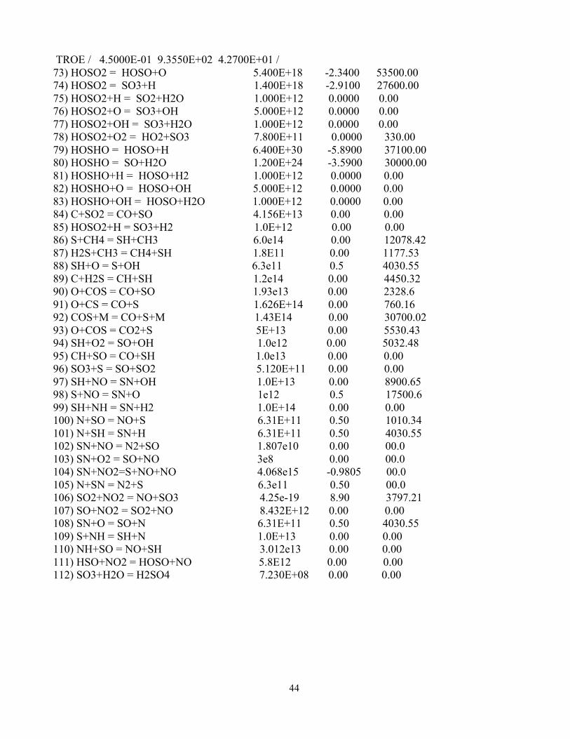
44
TROE / 4.5000E-01 9.3550E+02 4.2700E+01 / 73) HOSO2 = HOSO+O 5.400E+18 -2.3400 53500.00 74) HOSO2 = SO3+H 1.400E+18 -2.9100 27600.00 75) HOSO2+H = SO2+H2O 1.000E+12 0.0000 0.00 76) HOSO2+O = SO3+OH 5.000E+12 0.0000 0.00 77) HOSO2+OH = SO3+H2O 1.000E+12 0.0000 0.00 78) HOSO2+O2 = HO2+SO3 7.800E+11 0.0000 330.00 79) HOSHO = HOSO+H 6.400E+30 -5.8900 37100.00 80) HOSHO = SO+H2O 1.200E+24 -3.5900 30000.00 81) HOSHO+H = HOSO+H2 1.000E+12 0.0000 0.00 82) HOSHO+O = HOSO+OH 5.000E+12 0.0000 0.00 83) HOSHO+OH = HOSO+H2O 1.000E+12 0.0000 0.00 84) C+SO2 = CO+SO 4.156E+13 0.00 0.00 85) HOSO2+H = SO3+H2 1.0E+12 0.00 0.00 86) S+CH4 = SH+CH3 6.0e14 0.00 12078.42 87) H2S+CH3 = CH4+SH 1.8E11 0.00 1177.53 88) SH+O = S+OH 6.3e11 0.5 4030.55 89) C+H2S = CH+SH 1.2e14 0.00 4450.32 90) O+COS = CO+SO 1.93e13 0.00 2328.6 91) O+CS = CO+S 1.626E+14 0.00 760.16 92) COS+M = CO+S+M 1.43E14 0.00 30700.02 93) O+COS = CO2+S 5E+13 0.00 5530.43 94) SH+O2 = SO+OH 1.0e12 0.00 5032.48 95) CH+SO = CO+SH 1.0e13 0.00 0.00 96) SO3+S = SO+SO2 5.120E+11 0.00 0.00 97) SH+NO = SN+OH 1.0E+13 0.00 8900.65 98) S+NO = SN+O 1e12 0.5 17500.6 99) SH+NH = SN+H2 1.0E+14 0.00 0.00 100) N+SO = NO+S 6.31E+11 0.50 1010.34 101) N+SH = SN+H 6.31E+11 0.50 4030.55 102) SN+NO = N2+SO 1.807e10 0.00 00.0 103) SN+O2 = SO+NO 3e8 0.00 00.0 104) SN+NO2=S+NO+NO 4.068e15 -0.9805 00.0 105) N+SN = N2+S 6.3e11 0.50 00.0 106) SO2+NO2 = NO+SO3 4.25e-19 8.90 3797.21 107) SO+NO2 = SO2+NO 8.432E+12 0.00 0.00 108) SN+O = SO+N 6.31E+11 0.50 4030.55 109) S+NH = SH+N 1.0E+13 0.00 0.00 110) NH+SO = NO+SH 3.012e13 0.00 0.00 111) HSO+NO2 = HOSO+NO 5.8E12 0.00 0.00 112) SO3+H2O = H2SO4 7.230E+08 0.00 0.00


THE LESLIE HARRIS CENTRE OF REGIONAL POLICY AND DEVELOPMENT1st Floor Spencer Hall, St. John’s, NL Canada A1C 5S7Tel: 709 864 6170 Fax: 709 864 3734 www.mun.ca/harriscentre