1 | P a g e

ESSAYS ON THE FISCAL ASPECTS OF TRADE LIBERALISATION

DACIA ASTAIRE SAMUELS, MSc.

Thesis submitted to the University of Nottingham

for the degree of Doctor of Philosophy

JULY 2017

2 | P a g e

ABSTRACT

This thesis comprises a series of three studies that explore the impact of trade

reform on fiscal revenue. Two of the studies use cross-country econometric

methods and the third utilizes a partial equilibrium approach to analyse the

impact of trade liberalisation on tax revenue and welfare in Jamaica. The first

study examines the impact of trade liberalisation on total revenue and trade

tax revenue as a share of GDP across countries, explores heterogeneity within

the sample (in particular the extent to which a country’s level of development

influences variations in the effects of trade liberalisation) and utilises

alternative indicators of openness to determine if the findings of the model are

sensitive to the indicator of openness used. The study finds that, in the case

of the openness index used by Khattry and Rao (2002), international trade tax

and total tax revenue as a percent of GDP are likely to rise as an economy

becomes less open. In contrast, when trade as a percent of GDP is used as the

indicator of openness, the results show a positive relationship between

openness, and trade and total tax revenue as a share of GDP. The results also

suggest that international trade tax revenue tends to fall over time as a country

develops. The second study uses events analysis to examine the same issue.

There is weak evidence that trade reform has positive revenue effects in the

long-run; however, there may be negative impacts within a year of reform.

The third study explores the impact of trade liberalisation under the EU-

CARIFORUM Economic Partnership Agreement (EPA) on Jamaica by simulating

different tariff reform scenarios and comparing the results with the end term

EPA as negotiated. It finds that small countries can devise appropriate

strategies to mitigate potential negative fiscal effects of trade reform such as

scheduling tariff reductions for high revenue items later in the reform process.

It also finds that there is often a trade-off between revenue and welfare, which

makes welfare increasing and revenue enhancing outcomes difficult to

achieve.

3 | P a g e

ACKNOWLEDGEMENTS

I must express sincere gratitude to my supervisor, Professor Chris Milner, for

his guidance over the period of my thesis. I have learnt so much from him that

I will apply throughout my career. I must also thank Dr. Peter Wright, formerly

of the University of Nottingham, for providing the data for the dummy

variables used in the events analyses. Additionally, I thank Jamaica Customs

for providing the trade data for Jamaica that I utilised in Chapter 4 of the thesis

and Mr. Olivier Jammes of the World Bank for providing a version of TRIST that

was compatible with my computer. Finally, I wish to thank my family and

friends who encouraged me throughout the process of completing the thesis.

4 | P a g e

TABLE OF CONTENTS Abstract ......................................................................................................................... 2

Acknowledgements ...................................................................................................... 3

List of Figures ................................................................................................................ 6

List of Tables ................................................................................................................. 7

Acronyms ...................................................................................................................... 9

1. Introduction ........................................................................................................... 10

1.1 Structure of the thesis ...................................................................................... 11

2. THE FISCAL IMPLICATIONS OF TRADE LIBERALISATION ...................................... 13

2.1 Introduction ...................................................................................................... 13

2.2 Literature Review .............................................................................................. 14

2.3 Data Analysis ..................................................................................................... 27

2.5 Addressing Endogeneity in the Model .............................................................. 46

2.6 Conclusions ....................................................................................................... 50

Appendix 2A - Countries in Equations 1 and 2............................................................ 53

Appendix 2B: Correlation Matrices ............................................................................. 54

3. Events Analysis of the Impact of Trade Liberalisation ............................................ 55

3.1 Introduction ...................................................................................................... 55

3.2 Measuring Events .............................................................................................. 56

3.3 Data Analysis ..................................................................................................... 58

3.4 Regression Model ............................................................................................. 63

3.5 Regression Results ............................................................................................ 68

3.6 Heterogeneity within the model....................................................................... 79

3.7 Conclusions ....................................................................................................... 93

Appendix 3A - Countries and Year of Liberalisation Event in Events Analysis ............ 97

4. REVENUE AND WELFARE EFFECTS OF THE EU-CARIFORUM EPA ON JAMAICA AND

THE DESIGN OF WIRE TARIFF REFORM OUTCOMES ........................................... 98

4.1 Introduction ...................................................................................................... 98

4.2 Literature Review ............................................................................................ 102

4.3 Jamaica – Trade and Tariff Profile................................................................... 113

4.4 Methodology ................................................................................................... 121

4.5 Tariff Liberalisation Scenarios ......................................................................... 131

5 | P a g e

4.6 Welfare Increasing and Revenue Enhancing (WIRE) Tariff Reform Outcomes

.............................................................................................................................. 151

4.7 Conclusions ..................................................................................................... 159

Appendix 4A – Tariff Line Descriptions ..................................................................... 162

Appendix 4B – Detailed Results for WIRE Tariff Reform Scenarios .......................... 163

5. Conclusions ........................................................................................................... 166

5.1 Limitations of the study and opportunities for further research ................... 168

Bibliography .............................................................................................................. 169

6 | P a g e

LIST OF FIGURES

Figure 2-1: Share of Total Tax Revenue in GDP……………………………………………………….28 Figure 2-2: Share of Trade Tax Revenue in GDP………………………………………………………29 Figure 2-3: Ratio of Trade Tax Revenue to Total Tax Revenue………………………………..29 Figure 2-4: Scatterplot TRgdp and Urbpop……………………………………………………………..33 Figure 2-5: Scatterplot TRgdp and lnpop…………………………………………………………………33 Figure 2-6: Scatterplot TRgdp and lnGDPpc…………………………………………………………….33 Figure 2-7: Scatterplot TRgdp and Dep……………………………………………………………………33 Figure 2-8: Scatterplot TRgdp and tt……………………………………………………………………….33 Figure 2-9: Scatterplot TTgdp and lnGDPpc…………………………………………………………….34 Figure 2-10: Scatterplot TTgdp and DTaxdgp………………………………………………………….34 Figure 2-11: Scatterplot TTgdp and Trade………………………………………………………………35 Figure 2-12: Augmented Component Plus Residual Plot for lnGDPpc, Equation 1…..41 Figure 3-1: Scatterplot of Total Trade Tax Revenue as a Share of GDP and the World Bank Dummy………………………………………………………………………………………………………….59 Figure 3-2: Scatterplot Total Trade Tax Revenue as a Share of GDP and the Sachs-Warner1 Dummy……………………………………………………………………………………………………60 Figure 3-3: Scatterplot Total Trade Tax Revenue as a Share of GDP and the Sachs-Warner2 Dummy……………………………………………………………………………………………………61 Figure 3-4: Scatterplot Total Trade Tax Revenue as a Share of GDP and the Dean1 Dummy…………………………………………………………………………………………………………………..62 Figure 3-5: Scatterplot Total Trade Tax Revenue as a Share of GDP and Dean2 Dummy…………………………………………………………………………………………………………………..62 Figure 3-6: Minimum Ratio of Export to Total Trade Taxes (1972-1990)…………………86 Figure 3-7: Ratio of Export Taxes to Total Trade Taxes (1972 and 1989)…………………87 Figure 4-1: Jamaica's Top Ten Imports in 2011……………………………………………………. 114 Figure 4-2: Jamaica’s Main Trading Partners in 2011 ............................................... 114 Figure 4-3 Jamaican Imports from EU 2011 .............................................................. 115 Figure 4-4 Jamaican Exports to the EU 2011 ............................................................ 116 Figure 4-5: Effect of an EPA with Perfect Substitution ............................................. 129 Figure 4-6: Scenario 1 Trade Creation and Diversion estimates............................... 136 Figure 4-7: Scenario 1 Change in Tariff and Total Tax Revenue ............................... 137 Figure 4-8: Scenario 1 Net Welfare Effects ............................................................... 137 Figure 4-9: Scenario 2 Trade Diversion and Trade Creation Estimates…………………. 138 Figure 4-10: Scenario 2 Change in Tariff and Total Tax Revenue……………………………140 Figure 4-11: Scenario 2 Net Welfare Effect .............................................................. 139 Figure 4-12: Collected Applied Tariff Rate by ISIC Sector Scenarios 1 and 2 ............ 140 Figure 4-13: Comparison of Initial Applied Tariff Rates and Statutory Tariff Rates 153 Figure 4-14: Comparison of the Initial Applied Tariff Rate and Revised Rates under Scenario 3b ............................................................................................................... 154 Figure 4-15: Initial Applied Tariff Rates and Maximum Rates under Scenario 4 ...... 155 Figure 4-16: Applying a uniform tariff rate to the collected tariff rate structure..... 156

7 | P a g e

LIST OF TABLES

Table 2-1: Variable Means by Country and Year Groupings (1972-2006) ………………..32 Table 2-2: Regression Results, TRgdp and TTgdp…………………………………………………….38 Table 2-3: Comparison of Khattry and Rao Equation 1 Coefficients with Eq. 1 Regression Estimates, TRgdp………………………………………………………………………………….39 Table 2-4: Comparison of Khattry and Rao Equation 2 (TTgdp) Coefficients with Regression Results………………………………………………………………………………………………….39 Table 2-5: Regression Results with the square of Per capita GDP, TRgdp and TTgdp……………………………………………………………………………………………………………………..41 Table 2-6: Equation 1 Regression by Country Group, TRgdp……………………………………42 Table 2-7: Equation 2 Regression by Country Group, TTgdp……………………………………43 Table 2-8: Regressions without high income countries, TRgdp and TTgdp………………45 Table 2-9: Regressions using 1-year lag of Trade, TRgdp and TTgdp……………………….47 Table 2-10: Equation 2 without Trade, TTgdp…………………………………………………………49 Table 2-11: Regressions using 3-year lag of Trade, TRgdp and TTgdp……………………..50 Table 2-12: Correlation Matrix for Equation 1…………………………………………………………54 Table 2-13: Correlation Matrix for Equation 2…………………………………………………………54 Table 3-1: The Determinants of Tax Revenue as a Share of GDP (TRgdp) – Average Post Reform Effect………………………………………………………………………………………………………….69 Table 3-2: The Determinants of Tax Revenue as a Share of GDP (TRgdp) – Immediate Reform Impact………………………………………………………………………………………………………71 Table 3-3: The Determinants of Trade Tax Revenue as a Share of GDP (TTgdp) – Average Post Reform Effect ........................................................................................ 72 Table 3-4: The Determinants of Trade Tax Revenue as a Share of GDP (TTgdp) – Immediate Reform Impact .......................................................................................... 75 Table 3-5: Comparison of Regression Results across Models for the Share of Total Tax Revenue in GDP .......................................................................................................... 76 Table 3-6: Comparison of Regression Results across Models for the Share of Total Trade Tax Revenue in GDP .......................................................................................... 77 Table 3-7: The Determinants of Tax Revenue as a Share of GDP by Income Group – Average Post Reform Effect ........................................................................................ 80 Table 3-8: The Determinants of Tax Revenue as a Share of GDP by Income Group –Immediate Reform Impact .......................................................................................... 81 Table 3-9: The Determinants of Trade Tax Revenue as a Share of GDP by Income Group – Average Post Reform Effect ..................................................................................... 82 Table 3-10: The Determinants of Trade Tax Revenue as a Share of GDP by Income Group - Immediate Reform Impact ............................................................................ 83 Table 3-11: Ratio of Export Taxes to Total Trade Taxes in Descending Order of the Highest Value over 1972-1975 – Top 15 in Sample .................................................... 87 Table 3-12: The Determinants of Tax Revenue as a Share of GDP by Export Tax Revenue to Total Trade Tax Revenue Ratio – Average Post Reform Effect ................ 88 Table 3-13: The Determinants of Tax Revenue as a Share of GDP by Export Tax Revenue to Total Trade Tax Revenue –Immediate Reform Impact............................ 89 Table 3-14: The Determinants of Trade Tax Revenue as a Share of GDP by Export Tax Revenue to Total Trade Tax Revenue – Average Post Reform Effect ......................... 90 Table 3-15: The Determinants of Trade Tax Revenue as a Share of GDP by Export Tax

Revenue to Total Trade Tax Revenue - Immediate Reform Impact……………91

Table 4-1: Jamaica Tariff Profile……………………………………………………………………………119

8 | P a g e

Table 4-2: Jamaica TRIST Summary Data .................................................................. 120 Table 4-3: Trade and Revenue Impact of Full Liberalisation for Jamaica under the EU-CARIFORUM EPA ....................................................................................................... 134 Table 4-4: Change in Pattern of Imports – Scenarios 1 and 2................................... 135 Table 4-5: Revenue and Welfare Effects of the EU-CARIFORUM EPA for Jamaica - Scenarios 1 and 2 ...................................................................................................... 135 Table 4-6: Top 10 Industries by Imports Value Change for Scenario 1 ..................... 143 Table 4-7: Top 10 Industries by Imports Value Change for Scenario 2 ..................... 144 Table 4-8: Average Collected Applied Rates ............................................................. 145 Table 4-9: Top 25 Tariff lines by Revenue Loss with Change in Imports and Welfare (US$).......................................................................................................................... 147 Table 4-10: Proportion of EU imports in each tariff line in total EU imports Pre and Post Scenario 1 .......................................................................................................... 148 Table 4-11: Full Liberalisation of EU Imports vs End term EPA with Excluded Products .................................................................................................................................. 149 Table 4-12: Revenue and Welfare Impacts of Linear Cuts in the Collected Applied Tariff Rate (US$ million) ..................................................................................................... 157 Table 4-13: Revenue and Welfare Impacts of Maximum Collected Applied Tariff Rates (US$ million) .............................................................................................................. 157 Table 4-14: Revenue and Welfare Impacts of Uniform Collected Applied Tariff Rates (US$ million) .............................................................................................................. 158 Table 4-15: Change in Pattern of Imports - Details .................................................. 163 Table 4-16: Revenue and Welfare Impacts of Linear Cuts of 5% and 10% in the Collected Applied Tariff Rate (US$) Details .............................................................. 164 Table 4-17: Revenue and Welfare Impacts of Maximum Collected Applied Tariff Rates of 15%, 20%, 30%, and 32% (US$) Details ................................................................ 164 Table 4-18: Revenue and Welfare Impacts of Uniform Collected Applied Tariff Rate of 3.3%, 4.3%, 4.5%, and 7.4% (US$) Details ................................................................ 165

9 | P a g e

ACRONYMS

CARICOM Caribbean Community

CARIFORUM CARICOM member countries plus Cuba and the

Dominican Republic

CET Common External Tariff

CGE Computable General Equilibrium

CREs Compensated Radial Elasticities

EAC East African Co-operation

EPA Economic Partnership Agreement

EU European Union

FTA Free Trade Area

GCT General Consumption Tax

GDP Gross Domestic Product

GMM Generalised Method of Moments

GOJ Government of Jamaica

IMF International Monetary Fund

LDCs Least Developed Countries

MFN Most Favoured Nation

NTBs Non-Tariff Barriers

OECD Organisation for Economic Cooperation and

Development

QRs Quantitative Restrictions

ROW Rest of the World

SMART Single Market Partial Equilibrium Tool

SSA Sub-Saharan Africa

TPR Trade Policy Review

TRIST Trade Impact Simulation Tool

VAT Value Added Tax

WIRE Welfare Increasing and Revenue Enhancing Reforms

WITS World Integrated Trade Solution

WTO World Trade Organisation

10 | P a g e

1. INTRODUCTION

Studies on the impact of trade liberalisation often focus on its effects on

welfare. While this normative perspective is important, it is also necessary to

consider the potential impact of trade reform on fiscal revenue. This issue is

of primary concern to policymakers, particularly in developing country

contexts where sources of fiscal revenue sources may be limited and hence,

tariff revenue may be a major source of fiscal revenue. Therefore, although

there is widespread recognition and acceptance among economists that tariffs

are a second-best method of achieving fiscal policy objectives (Michael et al.

(1993)), trade liberalisation is often feared for possible negative fiscal

consequences due to the potential for loss of revenue as a result of tariff

reform.

Additionally, there are political economy concerns that impact the ability of a

government to implement tariff reform as competing interest groups lobby to

gain the outcome that is in their best interest. In many instances, the benefits

of a tariff tend to be concentrated on certain key interest groups who lobby

for their continuation while the costs are often widely dispersed (Bliss (1987)).

Therefore, it often proves difficult for governments to push through reforms

as there is likely to be an inherent bias for the continuation of tariffs. It is

therefore incumbent on policymakers to balance these competing

considerations and at the same time ensure that the ultimate trade reform

outcome is positive for the country – whether in terms of fiscal revenue,

welfare, or both.

A review of available studies on the fiscal and welfare effects of trade reform

reveal that there are relatively few on the fiscal aspects and more on the

welfare effects of trade reform. In addition, a lot of these studies focus on a

theoretical rather than empirical assessment of these issues. This thesis adds

to the empirical studies on both these aspects of trade reform, with the fiscal

effects being a primary focus of two chapters.

While most studies on the fiscal aspects of trade reform measure trade tax

revenue at an aggregate level, it is useful to analyse the impact of trade reform

on the different components of trade tax revenue so that reform measures are

appropriately structured. An understanding of what drives the change in trade

tax revenue – whether mainly import taxes, export taxes, and/or other

components - can identify priority areas for reform and inform the order of

implementation of reform measures. Conceivably, one may observe a

reduction in total trade taxes as a result of tariff reform and yet when the total

figure is dissected, there may have been a net increase in import duties, and a

reduction in export duties and exchange taxes. This type of analysis is

particularly relevant when comparing the aggregate measure of total trade

11 | P a g e

taxes across countries with varying tax systems as it is likely to be more difficult

to determine the principal components impacted by the reform; for example,

whether one is likely to observe mainly changes in import duties, and/or

changes in export duties. In this context, the specific research questions that

this thesis will investigate are:

• How does trade liberalisation affect total tax revenue, and

international trade tax revenue in particular?

• Are there variations in the impact of trade liberalisation depending on

a country’s level of economic development or dependence on specific

taxes, such as export taxes?

• Are the findings of the model sensitive to the indicator of openness

used?

In addition to consideration of the fiscal effects, the welfare implications are

also an important aspect of trade reform, particularly as the gains of

liberalisation are often expressed in terms of an improvement in consumer

welfare. For policymakers, a primary concern is how to structure trade

reforms to obtain the desired outcomes for tariff revenue and welfare; for

example, an aim of trade reform may be revenue neutrality and positive

welfare effects. Most of the studies on the fiscal and welfare effects are

analysed in a stylised first-best framework of full liberalisation that is not

particularly realistic for policy makers. This thesis extends the analysis by

examining this issue in a second-best framework – where there is partial

liberalisation under a free trade agreement but tariffs remain on Rest of the

World (ROW) imports. For detail and depth of analysis, it is useful to examine

this issue at an individual country level. A suitable case study for consideration

is that of a small open economy (Jamaica) in a free trade agreement (EU-

CARIFORUM Economic Partnership Agreement (EPA)). In this second-best

setting, one can assess various reform scenarios and their likely impact on

revenue and welfare. Through a partial equilibrium approach, this thesis will

answer the questions:

• How can Jamaica design Rest of the World (ROW) tariffs to minimise

possible negative fiscal and welfare impacts of the EU-CARIFORUM

EPA?

• Can Jamaica achieve Welfare Increasing and Revenue Enhancing

(WIRE) outcomes in this context?

1.1 Structure of the thesis

In order to answer these research questions, the thesis starts by examining the

question of whether trade liberalisation necessarily results in revenue

12 | P a g e

depletion and assesses the likelihood that countries will recoup international

trade tax revenue losses by changes in other tax sources, such as domestic

taxes (Chapter 2). Two equations are estimated, using fixed effects panel

regression analysis, with international trade tax revenue as a share of GDP, and

total trade tax revenue as a share of GDP as the dependent variables. The

regressions include relevant socio-economic indicators, such as the level of

urbanisation, per capita income, population size, and the age-dependency

ratio. These equations are estimated at an aggregate level and then by country

groups based on a country’s level of development in order to assess how

liberalisation may impact each country differently. Accounting for possible

endogeneity issues, the study then goes on to vary the model by using a more

traditional indicator of openness, trade as a per cent of GDP.

Chapter 3 continues the analysis within an events framework based on the fact

that trade liberalisation is often driven by economic shocks and externally

imposed under loan agreements with multilateral lending institutions. We can

therefore examine the impact of trade liberalisation through changes in key

fiscal variables, such as total tax revenue and trade tax revenue as a share of

GDP, in the period before and after liberalisation. This chapter also explores

the issue of heterogeneity within the sample, in regard to varying levels of

development among countries and the treatment of export taxes by individual

countries.

Chapter 4 takes the analysis further and examines the tariff revenue, trade

creating, trade diverting and welfare effects of full liberalisation under the EU-

CARIFORUM EPA at the product level for Jamaica. It also examines the

different effects of utilising statutory tariff rates versus collected tariff rates in

the analysis and analyses how Jamaica may adjust Common External Tariffs on

ROW imports after implementation of the EPA in order to address concerns

about tariff revenue depletion and welfare loss, for example. It then examines

the feasibility of achieving welfare increasing and revenue enhancing (WIRE)

outcomes for tariff adjustments on ROW imports post-EPA.

The thesis then concludes in Chapter 5 where the main findings and higher-

level conclusions, along with their limitations, are identified.

13 | P a g e

2. THE FISCAL IMPLICATIONS OF TRADE LIBERALISATION

2.1 Introduction

The impact of trade liberalisation on fiscal revenue has long been a concern for

policymakers and researchers. Their main concerns include exploring whether

adverse revenue effects necessarily accompany trade liberalisation and

possible mitigating measures where adverse effects are observed. In addition,

researchers have analysed the factors that are likely to influence the degree of

revenue loss such as a country’s level of development, the degree of

urbanisation and the degree of openness of its economy.

In order to investigate these issues, researchers have utilised various

methodologies, ranging from cross-section regression analysis to more recent

efforts to take advantage of both time and group variations with the use of

panel datasets. Limitations of some of these models, such as cross-country

simple linear regression analysis, include the inability to examine changes in

the variables over time which is especially important in the context of

international trade given that trade liberalisation usually has lagged effects.

Additionally, some models (including those that use panel datasets) have

undesirable features such as endogeneity, depending on the indicators used

to measure variables such as openness and international trade taxes.

This essay examines the question of whether trade liberalisation necessarily

results in revenue depletion and the likelihood that countries will recoup

international trade tax revenue losses by changes in other tax sources, such as

domestic taxes. Using fixed effects panel regression analysis, with

international trade tax revenue as a share of GDP, and total tax revenue as a

share of GDP as the dependent variables, the study estimates the relationship

between openness and international trade tax revenue and total tax revenue

as a share of GDP. 1 The regressions include relevant socio-economic

indicators, such as the level of urbanisation, per capita income, population

size, and the age-dependency ratio. The concept of openness is explored by

using alternative measures - an openness index (Khattry and Rao (2002)) and

the one-year lag of Trade as a share of GDP). The openness index is

endogenous to the model and is therefore unlikely to provide reliable

estimates. The lag of trade as a share of GDP does not face this criticism as it

is less likely to be contemporaneously correlated over time with trade and total

1 International trade tax revenue comprise taxies imposed on goods and services

entering a customs territory, including import duties, export duties, profits of export

or import monopolies, exchange profits, and exchange taxes. Total tax revenue refers

to all compulsory transfers to the central government. (IMF Government Financial

Statistics Database - 2014)

14 | P a g e

tax revenue as a share of GDP. In addition, the study explores heterogeneity

within the model by estimating the equations by country groups based on a

country’s level of development in order to assess how liberalisation may

impact each country differently. Before delving into the data analysis and

regression results, the next section provides a review of key literature on trade

liberalisation and its possible impact on fiscal revenue.

2.2 Literature Review

The Literature Review first provides an overview of the relevant theoretical

underpinnings for tariff formulation and the principles of taxation in general.

This section also provides a rationale for the imposition of tariffs and their

impact on domestic and global welfare. It then goes on to focus specifically on

the factors that influence the level of trade taxes (of which revenue earned

from tariffs comprise the vast majority) in total tax revenue and as a

percentage of GDP. Following this discussion, it examines the impact of trade

liberalisation on tax revenue, taking account of issues such as the impact on

domestic tax revenue, and export taxes. It also provides an overview of the

methodologies that have been used thus far to investigate the nature of the

relationship between trade tax revenue and trade liberalisation. Finally, it

concludes by summarising the main findings from the literature review and

charts the layout of the rest of the chapter.

2.2.1 Theoretical Foundations

In order to have a complete understanding of the issues surrounding the

impact of trade liberalisation on trade taxes, this section assesses the factors

that influence the amount of trade taxes that a government can raise in order

to gauge the final revenue outcome from liberalisation. In this context, there

are often conflicting effects at play; for example, some effects of tariff

liberalisation depend on the elasticity of substitution between imports and

their domestic substitutes and it is therefore difficult to predict the final reform

outcome. The section then goes on to trace the likely impact of trade

liberalisation on key variables as identified in the economic literature.

(a) Factors Influencing the Share of Trade Tax Revenue in Total Revenue and in

GDP

The share of trade tax revenue in total government revenue and in GDP varies

between countries due to several factors. It may be observed that the share

of trade tax revenue in GDP varies with a country’s level of economic

15 | P a g e

development. It is argued that as a country becomes more developed, tax

systems mature, administrative experience and efficiencies are gained, and

thus other sources of revenue become much more significant than trade tax

revenue. Greenaway (1980) attributes this inverse relationship between trade

tax revenue and the level of economic development to a country’s level of

industrialisation which gives rise to greater need for cash transactions; low

income elasticity of trade tax revenue; changes in the composition of imports

demanded as economies develop, towards intermediate capital goods; the

maturity of infant industries which causes less revenue to be earned from their

import substitutes; and the general disinclination of industrialised countries to

use trade taxes as a source of revenue.

One can also assume that the degree of openness of an economy provides an

indication of potential revenue earnings from taxes on trade.2 One can expect

a positive correlation between trade tax revenue and the size of the traded

goods sector as, ceteris paribus, the more goods that are subjected to import

duties and export taxes, for example, the more earnings a government is likely

to receive. In a general equilibrium context, however, where there is imperfect

competition, the imposition of additional duties and taxes on imports may

induce changes in consumer behaviour such as increased spending on

domestic substitutes. In this case, even where producers of domestic

substitutes take the opportunity to increase product margins, the increase may

be less than the full amount of the tariff; hence, the final outcome is

unpredictable. Moreover, in many developing countries, there is a difference

in the average nominal tariff and the collected tariff rate due to the number of

exemptions available.

In its common manifestation, trade liberalisation involves the reduction and/or

removal of duties on imports entering into a country. One would therefore

expect that the amount of trade tax revenue earned by a government would

vary depending on the rates of import duties, export taxes, and stamp duties,

for example. Khattry and Rao (2002) posit that the direct effect of tariff

liberalisation is dependent on whether or not initial tariffs were relatively high

and above their revenue-maximising levels. If they are not above their

revenue-maximising levels, tariff liberalisation will increase tariff revenue; if

they are, then tariff liberalisation will lead to declining revenue. They also

point out that the indirect effects of tariff liberalisation depend on the

elasticity of substitution between imports and their domestic substitutes. It is

noted that in general the net change cannot be predicted.

2 For a more intensive discussion, see Greenaway (1980), Greenaway and Milner

(1991) and Cole (1992)

16 | P a g e

Where a country is heavily dependent on primary agricultural products, there

may be increased likelihood of the presence of export taxes on products from

the traditional export sectors (Burgess and Stern (1993)). As noted by

Greenaway and Milner (1991) and Khattry and Rao (2002), the removal of

export taxes is expected to reduce tax yield but other export enhancing

measures could be pursued such as tax rebates which may encourage

increased exports and hence, greater earnings and direct tax yields from

sources such as income tax. Export taxes, however, are a negligible source of

revenue for the vast majority of countries currently.

Changes in the exchange rate can affect the share of trade taxes in total

revenue and GDP. A depreciation of the real exchange rate makes imports

more expensive in domestic currency terms and can therefore reduce the

quantity of imports demanded and increase demand for domestic import

substitutes. The precise effect depends on the relevant price elasticity of

demand for imports and the price elasticity of supply for import substitutes. If

price elasticity of demand for imports is relatively inelastic then the

government would expect to see increased revenue earnings from tariffs.

Greenaway and Milner (1991) note that this is often the case for capital goods

and intermediates for Less Developed Countries. On the other hand,

consumer goods and food items with domestic substitutes tend to have high

elasticity. Currency depreciation also has a positive effect on exports which

may lead to increased revenue from taxes on income. The net impact

therefore depends on these competing considerations (Agbeyegbe et al.

(2006)).

Khattry and Rao (2002) point to the structural constraints faced by many

developing countries in relation to their level of urbanization and age-

dependency ratios. In Lewis’ (1954) model of structural change, an economy

becomes more urbanised as it develops. This increases its need for and

capacity to tax as the urban population demands provision of additional public

services and provides a targeted tax base through the economic activity

generated. In many developing countries where the rural economy tends to

be the dominant sector, economic activity tends to be less concentrated and

mostly informal in nature, which makes tax assessment difficult. Therefore, in

some cases, governments levy taxes on agricultural exports. In addition, the

high age-dependency ratios in many countries mean that the tax base is

smaller than in developed countries which tend to have lower age-dependency

ratios.

The factors discussed above constitute the explanatory variables that influence

changes in trade taxes and total taxes. The age dependency ratio, the level of

urbanization, and per capita income account for structural characteristics in

the economy that determine a country’s taxable base. The inclusion of the

exchange rate in the trade tax revenue model accounts for the possible impact

17 | P a g e

of changes in monetary policy on exports and imports. Additionally, one

should be mindful that the final impact of trade liberalisation on fiscal revenue

is also dependent on other factors such as a country’s existing tariff structure

and where tariffs are located in relation to their revenue-maximising levels,

the availability of domestic substitutes and their elasticities of supply and

demand, and other structural constraints faced by individual economies.

(b) The Impact of Trade Liberalisation

The likely impact of trade liberalisation can be assessed in terms of the

measures that comprise the reform process. This section sets out the a priori

expectations of reforms, such as the removal of quantitative restrictions; tariff

reform, including liberalisation and reduction in dispersion; domestic tax

revenue; and exchange rate adjustment, on fiscal revenue. One of the most

frequent components of reform has been the tariffication of quantitative

restrictions (QRs). The replacement of quantitative restrictions provides an

additional source of tax revenue but the extent to which this happens is

dependent on the impact of tariffs on domestic prices and hence on domestic

demand for the affected products. It may be the case that the increase in prices

reduces demand and hence the volume of trade, thereby affecting the revenue

outcome. Ebrill et al. (1999) note that the impact of changes in quantitative

restrictions is dependent on the nature of the restriction itself and the

administrative capabilities of the countries implementing such reform. For

example, removing quotas on imports that are also subject to tariffs may lead

to an increase in revenue due to increased import volume.

Another plank of trade reform is tariff liberalisation. As already discussed, if

the initial tariff rate is above the revenue maximising rate, then any reduction

of the tariff is likely to increase trade tax revenue as the incentive for evasion

is lessened by the decrease or removal of the tariff and positive changes in

income may be induced. The converse is also true. If the initial tariff rate is

below the revenue maximising rate, then tariff reduction or elimination is likely

to result in a reduction in government revenue from trade taxes. The final

impact of tariff changes will therefore take account of the number of tariffs

above and below the tariff maximising rate, the magnitude of tariff changes,

and cross price elasticities of demand of imports and supply of import

substitutes. (See Greenaway and Milner (1991)).

Domestic tax revenue is also impacted by trade liberalisation. In many

developing countries, taxes on imported goods and services are an important

source of revenue. Indeed, these taxes are often levied on the tariff-inclusive

price. The removal of tariffs is therefore likely to reduce tax yield if the base is

eroded. Agbeyegbe et al. (2006) note, however, that the ultimate impact on

revenue yield has to take account of possible changes in import demand

18 | P a g e

(positive) and demand for import substitutes (negative) due to lower prices on

imports from removal of the tariff. Moreover, there may be long-term effects

on the tax base if liberalisation has a positive effect on economic growth.

Liberalisation measures often comprise a reduction in the dispersion of tariff

rates, and simplification of the tariff structure - with significant reduction or

removal of tax exemptions. Greenaway and Milner (1991) note that this

should be revenue-neutral but may have the positive effect of reducing the

incentive for tax evasion and improve administrative efficiencies and this will

have a positive effect on the revenue outcome. Ebrill et al. (1999) focus on the

relative importance of price elasticities of demand of imports impacted by the

reform measure. In this regard, it is argued that if reducing tariff dispersion

negatively affects effective rates of protection, then there is likely to be an

increase in imports and hence, increased revenue from trade taxes. In

addition, higher tariffs tend to be associated with goods that have higher price

elasticities of demand and if these tariffs are lowered, then the positive

revenue effect is likely to be reinforced through increased demand for these

products.

The removal of export taxes – another facet of liberalisation - may lead to a

reduction in trade tax revenue, ceteris paribus, if export volume is not affected

positively. Greenaway and Milner (1991) posit that one can expect an inverse

relationship between the significance of export taxes and the share of non-

traditional exports in total exports. This follows from the fact that export taxes

are applied to traditional exports in most cases and often allow for exemptions

so that producers are competitive.

In addition, one can expect some amount of exchange rate adjustment in many

trade reform packages. This can be analysed using the standard implications

of devaluation in a small open economy. Devaluation will increase the price of

imports but the extent to which this affects customs revenue depends on the

price elasticity of demand for imports. In addition, devaluation makes non-

tradeables more attractive to consumers than tradeables (which are now

relatively more expensive). This has a dual effect – there is likely to be a

decrease in customs revenue but also an increase in domestic indirect tax

revenues. Income taxes from tradeables may also rise as the now lower price

of exports in foreign markets should encourage greater demand for these

products; once producers respond, they should see increased earnings.

Khattry and Rao (2002) also discuss a terms of trade shock effect of

liberalisation. This would result from simultaneous trade liberalisation by

several developing countries which could lead to a glut on the market of similar

products. It is argued that this would depress the prices of these exports and

negatively affect export revenue and also income tax earnings from exporters.

This argument fails to take account, however, of the supply constraints and

19 | P a g e

rigidities faced by many developing countries which makes it very unlikely that

a significant number of these countries could increase production to take

advantage of the now more open economies simultaneously. Importantly, one

also needs to consider the demand for the products in question – more open

economies do not necessarily lead to increased demand for particular

products.

Agbeyegbe et al. (2006) also explore other impacts of trade liberalisation on

income and profit taxes. The short-run channel through which these impacts

are transmitted is via the changes in profits of importers and producers of

import substitutes. In addition, there may be long-run consequences if trade

liberalisation impacts on economic growth – positively or negatively – and

therefore on incomes and income tax liabilities. These general equilibrium

considerations are not the subject of this study but it is useful to bear in mind

that there are other possible indirect effects of trade liberalisation.

In addition to the nature of the trade reforms themselves, timing and

sequencing of reforms are also important considerations in determining the

final impact of trade liberalisation. Papageorgiou et al. (1990) argue that for

liberalisation to succeed it is best to implement reform measures quickly

rather than gradually – fast removal of QRs, and real depreciation of the

domestic currency. In addition, there should be a stable macroeconomic

environment. On the other hand, others such as Toye (2000) object to the “big

bang” approach and would rather see more gradual implementation of reform

measures with particular attention being paid to the sequencing of reforms

with stabilisation policies.

A common thread in the discussion above is that there can be no firm

expectation of the final impact of trade reform. Each country’s experience

depends on the its initial tariff structure before reform, price elasticities of

demand and supply for imports and domestic substitutes, the nature of trade

reforms, the pace and sequencing of trade reforms, and the extent of exchange

rate adjustment, if any. While recognizing that more detailed country-specific

analysis is necessary for any country contemplating trade reforms, cross-

country and panel analysis is useful to assess general patterns and trends over

time as countries have liberalised their economies. The next section examines

empirical studies conducted on the subject, with a view to identifying

appropriate methodologies for this research and the application of new or

different techniques where appropriate.

2.2.2 Methodologies

There is no single approach to determining the impact of trade liberalisation

on revenue. Most studies of the relationship between trade liberalisation and

20 | P a g e

changes in tax revenue utilise both correlation and regression analyses. The

regression models range from limited three variable cross-country regressions

(see Greenaway (1980) and Cole (1992)) to very extensive multi-variable

models with panel data (see Greenaway et al. (2002), Baunsgaard and Keen

(2005); and Khattry and Rao (2002), for example). One common thread in the

approaches taken by the various authors is careful selection of the trade

liberalisation variable. Indeed, one finds that in some instances the sensitivity

of results depends on the measure of liberalisation used. This section will

explore the models that have been used so far to examine the question of how

trade liberalisation impacts on growth and what are the best indicators of the

factors under consideration. It will also identify the limitations of some of the

indicators of trade liberalisation and models used and how researchers have

addressed these issues.

Measures of Trade Liberalisation and Openness

Researchers have investigated several approaches to measure the degree of

openness of an economy. Openness is often seen as being synonymous with

the outward orientation of an economy. Wacziarg (2001) lists three categories

of openness indicators – outcome measures, policy indicators and deviation

measures – in his study on the relationship between trade policy and economic

growth.

Outcome measures comprise indicators such as changes in trade volume and

composition that show the results of a country’s interaction with the global

market. The conventional measure of openness is exports plus imports, as a

percentage of GDP.3 However, some researchers have used the collected tariff

rate (import duties as a percentage of total imports) to measure openness.4 A

less accepted measure is the ratio of international trade taxes to international

trade used by Khattry and Rao (2002). The use of this measure gives rise to

issues of endogeneity where the share of international trade taxes in GDP is

used as the dependent variable. Moreover, as noted by Agbeyegbe et al.

(2006), this measure is limited in its application as a close relationship is not

directly observed between changes in one of the components of international

trade tax revenue, exports, and trade liberalisation.

More generally, the main drawback of outcome measures is the lack of a

strong theoretical framework for analysis as most theoretical papers utilise

trade policy measures such as tariffs (see David (2008) and Pritchett (1996)).

Wacziarg (2001) rejects the use of outcome measures, citing endogeneity

concerns relating to the use of outcome measures and variables such as

3 See Ebrill et al. (1999), Greenaway and Milner (1991), Greenaway et al. (2002) 4 For example, Ebrill (1999)

21 | P a g e

economic growth. He also notes that outcome measures include a gravity

component (trading patterns simply based on variations in geographical

location and country size) which would not be appropriate for a study that

seeks to capture the policy regime and that there are endogeneity concerns.

Other researchers such as Chang et al. (2009) have no issues with the use of

outcome measures. They use the volume of trade (the ratio of real exports

and imports to real GDP) to measure openness in their study on the effect of

openness and other variables on economic growth. Chang et al. (2009)

highlight that after controlling for country and time specific effects, the trade

to GDP ratio is a suitable proxy for trade policy. In addition, when the trade to

GDP ratio is replaced with average tariff rates to measure the robustness of

the model, the results remain the same.

Policy measures include the scheduled or applied tariff rates, non-tariff

barriers, and tariff revenues. Their levels indicate a country’s trade orientation

– low levels suggest openness to trade; high levels may suggest a

protectionist/anti-free trade leaning. Pritchett (1996) classifies these

indicators as “incidence” measures where there is direct assessment of the

trade policy measure. Wacziarg (2001) states that policy measures are likely

to influence outcome measures directly; for example, high tariff rates and the

existence of non-tariff barriers directly influence the amount of imports and

therefore, trade as a share of GDP. However, their utility may be limited based

on data availability and endogeneity concerns, depending on the variables in

the regression model.

Finally, deviation measures are based on the divergence of actual trade volume

from predicted free-trade levels, pioneered by Leamer (1988). The models are

based on gravity equations and factor endowments. The main drawback for

these models is the likelihood of omitted variables, including ones that reflect

policy stance and are highly correlated with gravity or endowment variables.

Arguing that it is best to combine variations in several measures to obtain an

indicator of openness that captures different dimensions of trade policy,

Wacziarg (2001) develops a Trade Policy Openness Index by measuring the

variation in trade shares attributable to various trade policy measures. The

ratio of exports plus imports to GDP is regressed on policy, gravity and

endowment variables. The components of the index are:

• The share of import duties in total imports

• The unweighted coverage ratio for the pre-Uruguay Round

time period published by UNCTAD

• Dummy variables based on country’s liberalization status,

using Sachs and Warner (1995)

22 | P a g e

The regression also includes the log of land area, log of population and the

growth rate of GDP per capita. The coefficients from the regression are used

as weights to construct a weighted average of these variables – the trade policy

openness index, equal to the portion of observed trade shares attributable to

the effective impact of trade policy. According to Wacziarg (2001), his

methodology avoids the problem of measurement error, as he constructs the

difference between potential and observed trade shares, and collinearity

between endowment, gravity and policy factors.

Also favouring the use of liberalisation indices, Greenaway et al. (2002) utilise

three indicators of liberalisation: indices developed by Dean et al. (1994), Sachs

and Warner (1995), and whether the country has a Structural Adjustment Loan

(SAL). Dean et al. (1994) derive a composite index of liberalisation to assess

when liberalisation occurred in their sample of thirty-two developing

countries. Reference is made to changes in tariffs, quotas, export measures,

and exchange rates. Sachs and Warner (1995) assess whether an economy is

open or closed based upon movements in non-tariff barriers and average tariff

levels; whether or not the country is socialist; the existence of state

monopolies over key exports; and the difference between the official and black

market exchange rates. All three indicators are entered as dummy variables

into a dynamic panel setting.

In addition to the measures cited above, there are other methods that assess

trade liberalisation and openness by comparing price levels across countries.

For example, Dollar (1992) estimates a cross-country index of real exchange

rate depreciation to estimate “outward-orientation”, using a measure of price

levels compiled by Summers and Heston for 121 countries. The measure is

similar to comparing purchasing power parities (PPP) across countries. The

main drawback of these measures, as noted by Balassa (1964) is the risk of

overvaluation of the exchange rate by PPP as developed countries tend to have

a comparative advantage in the traded goods sector (leading to higher

exchange rates) which imply that non-traded goods cost more in developed

countries when compared with less developing countries using the same

exchange rate, which is often not the case.

Estimation Techniques

Various techniques have been employed to explore the impact of trade

liberalisation on tax revenue. Ebrill et al. (1999) explore the impact of trade

liberalisation on revenue using fixed effects panel regression in two models. In

the first model, using a dataset of 27 countries over the years 1980-92, import

tax revenue as a share of GDP is determined by the import base and dummy

variables representing the reduction of tariffs, quantitative restrictions, and

23 | P a g e

export barriers. Other variables included in the estimating equation are

exports as a percentage of GDP, per capita income in 1990 U.S. dollars, dummy

variables for whether the country has a VAT, the achievement of Article VIII

status with the IMF ( possible indicator of a liberal trading regime as Article VIII

refers to the acceptance of the obligations of member states to avoid

discriminatory currency practices and restrictions on current payments for

international transactions), and the real exchange rate. Article VIII status with

the IMF is used as a liberalisation indicator since it is thought to be unrelated

to trade tax revenue and thus, uncorrelated with the error term, while at the

same time signalling a country’s commitment to free trade. The sample used

only includes countries that have undertaken liberalisation. Their results show

that tariff reductions have not had a significant impact on trade tax revenue

while changes in export taxes have had a significantly negative impact on trade

revenues. In addition, changes in QRs, using appropriate exchange rate

policies to support the reform process, and stimulating imports are likely to

have a positive and significant effect on trade tax revenue.

The second equation models trade tax revenue as a function of the collected

tariff rate, its square, and the other independent variables included in the first

model, excluding the liberalisation dummies, the import base, and exports as

a share of GDP. A quadratic form is estimated of the relationship between the

collected tariff rate and trade tax revenue to capture the idea of a revenue

maximising rate above which the collected tariff may actually decline. The

model confirms the existence of a revenue-maximising tariff rate.

Baunsgaard and Keen (2005) use similar fixed effects regressions to assess the

impact of trade liberalisation on tax revenue. However, the approach here is

different from those outlined previously in that the model seeks to estimate

the relationship between the costliness of collecting alternative forms of

revenue to trade taxes or the value of public spending, and trade liberalisation.

The dependent variable in this case is domestic tax revenue which is regressed

against a lagged dependent variable, trade tax revenue as a percentage of GDP

and a vector X that includes per capita GDP, openness, inflation, aid per capita,

and agriculture as a share of total value added. Similar to Ebrill et al. (1999),

Baunsgaard and Keen (2005) include a dummy variable reflecting whether the

country has a VAT in place, and have interaction terms of the VAT with

openness, and VAT with per capita GDP. In addition, a one-step Generalised

Method of Moment (GMM) regression is estimated to deal with issues of

endogeneity associated with trade tax revenue and bias from inclusion of the

lagged dependent variable. Their findings indicate that some trade tax

revenue lost as a result of trade liberalisation is likely to be recovered from

other sources and that countries with a VAT recover less revenue than those

without.

24 | P a g e

Agbeyegbe et al. (2006) use GMM estimation with an “orthogonal deviation

transformation” based on Arellano and Bover (1995) to estimate the

relationship between trade liberalisation and tax revenue for a panel data set

of 22 Sub-Saharan African countries over 1980-1996. An orthogonal deviation

transformation expresses each observation as the deviation from the average

of future observations in a sample for the same unit (for example, country) and

weights each deviation to standardise the variance. Where errors are serially

uncorrelated and homoskedastic initially, the transformed errors will also have

the same properties. The dependent variables are indicators such as total tax

revenue, trade taxes, and taxes on goods and services as a share of GDP. These

are regressed on the standard variables in the tax literature – per capita GDP,

the share of agriculture in GDP, the share of industry in GDP, the terms of

trade, inflation, government consumption, the real effective exchange rate,

net aid transfer, openness (share of international trade in GDP and share of

customs revenue as per cent of total imports), and a dummy variable for CFA

franc countries. They find that the openness indicators are not significant in

either equations, i.e., trade liberalisation does not have a significant impact on

trade tax revenues for this group of countries.

Khattry and Rao (2002) also use regression analysis to determine the factors

that influence tax revenue in general and trade tax revenue in particular. The

two models use panel data for 80 countries for the period 1970-98. For the

first model, the share of tax revenue in GDP is regressed on the natural log of

population size, the natural log of real GDP per capita, the age-dependency

ratio, the degree of urbanisation, and the index of openness. The second

equation looks at the effect of openness on customs revenue, using the same

independent variables as in the previous equation and adding the share of

domestic indirect taxes/GDP, the exchange rate, and the trade/GDP ratio.

Applying the same logic as Ebrill et al. (1999), the second equation includes a

quadratic form of the openness index because it is believed that rates of trade

taxation above a certain threshold may lead to declining tax revenues. The

openness variable selected is endogenous to the model, which limits one’s

ability to draw inferences from the estimation. Approaches to address

endogeneity include using lagged values, instrumental variables, 5 GMM

estimation,6 and event studies.7 An appropriate approach for this current

study is therefore to estimate an alternative specification of the model that

includes a lagged value of the traditional indicator of openness (Trade as a

share of GDP) to control for endogeneity and test the robustness of results,

using an extended data set. In addition, an event study will be done using the

liberalisation indicators identified in Greenaway et al. (2002) in a fixed effects

5 For example, Ebrill et al. (1999) 6 See Baunsgaard and Keen (2005), Agbeyegbe et al. (2006), and Chang et al. (2009). 7 Greenaway et al. (2002)

25 | P a g e

regression framework. The results from these two analyses will then be

compared to see if results are consistent across methodologies.

2.2.3 Conclusions

The literature on the impact of trade liberalisation on tariff revenue is diverse

but provides several starting points for analysis. Common variables that are

thought to affect the share of trade tax revenue among the studies researched

include GDP per capita, the share of agriculture, and domestic taxes as a

percent of GDP. The final effect of trade liberalisation depends on the

interplay of these factors, and the relative strength of each. It is accepted that

any assessment of the impact of liberalisation should include an analysis of

existing tariff levels and their location in relation to the revenue-maximising

rates. In addition, trade liberalisation also features less dispersion of tariff

rates, and the tariffication of quantitative restrictions. The analysis would

therefore need to take account of the impact of relative prices and demand for

final and intermediate goods as a result of changes in the price level due to

adjustments in the tariff structure.

Other issues that need to be assessed include: the pace of the liberalisation

process (rapid vs. gradual); the impact of exchange rate changes, usually

depreciation, that often accompany trade liberalisation; and the impact of

liberalisation on domestic tax revenues. With respect to the pace of

liberalisation, there is disagreement on whether a ‘big-bang’ approach is best

when implementing trade reform as it may speed up the adjustment process;

or whether a slower paced reform programme is best to give interest groups

time to adjust to incremental changes. For exchange rate changes, the impact

of depreciation is dependent on the elasticities of demand for exports and

imports and the availability of domestic substitutes. Domestic tax revenues

are also likely to be affected by trade liberalisation because most countries levy

taxes such as stamp duty on the tariff-inclusive price of the commodity; hence,

any reduction in that price is likely to affect revenue, ceteris paribus. Another

central question is the extent to which other sources can compensate for lost

trade tax revenue. Possible mitigating policies include measures to strengthen

the administrative capacity of tax institutions, and concomitant introduction

of other indirect taxes such as a consumption tax or a VAT.

Based on the preceding discussion, it is clear that a definitive outcome cannot

be predicted for the impact of trade liberalisation on particular countries.

However, the likely impacts can be assessed based on the experiences of

countries that have undergone liberalisation and any general trends that may

be observed. It is generally felt that a panel framework is best suited for this

analysis as it allows for the capturing of both cross-country and inter-temporal

effects. A key variable in any model estimating the impact of trade

liberalisation on fiscal revenue is the indicator of openness. All measures have

26 | P a g e

advantages and disadvantages, with liberalisation indices arguably being the

most recommended. While trade as a share of GDP is an outcome measure

and therefore not a direct indicator of trade policy, it can be argued that trade

ratios show the manifestation of trade policy. If an economy is inward-looking,

one should expect to see lower trade to GDP ratios, ceteris paribus, as

consumers and producers respond to high tariffs. Additionally, changes in

trade ratios depend on factors such as the structure of the economy, and

elasticities of demand and supply, and income elasticities. One criticism of the

measure is that in the case of developing countries that are dependent on the

exports of commodities, the share of imports in GDP tends to be relatively

stable over time but the share of exports in GDP is likely to vary based on

changes in the global market. The openness indicator may not fully capture

policy changes in this case where changes in trade as a share of GDP are driven

by exogenous factors on the global market that affect primary exports.

This research utilises a panel regression framework to analyse the impact of

trade reforms on fiscal revenue, similar to Baunsgaard and Keen (2005) and

Khattry and Rao (2002) and modifies the model to take into account

endogeneity concerns. The next section describes the data that will be used

in the model and presents trends in trade tax revenue and total tax revenue as

a share of GDP, the exchange rate, the level of urbanization, the age

dependency ratio, per capita income, population size, domestic taxes as a

share of GDP, the level of urbanization and trade (exports plus imports) as a

share of GDP.

27 | P a g e

2.3 Data Analysis

The data for the model are relevant tax and socio-economic indicators for 78

countries (see Appendix 2A) over the period 1970-2006. These include the

share of tax revenue in GDP, the share of trade tax revenue in GDP as

dependent variables. Independent variables are the exchange rate, the

natural log of population size, the dependency ratio, per capita GDP, domestic

taxes on goods and services as a share of GDP, the level of urbanisation, and

trade as a share of GDP.

2.3.1 Definition of key variables

In order to understand fully the composition of the model, it is necessary to

define the key variables. These definitions are from the International

Monetary Fund’s Government Financial Statistics (GFS) database.

Tax revenue (% of GDP): Tax revenue refers to compulsory transfers to the

central government for public purposes. Certain compulsory transfers such as

fines, penalties, and most social security contributions are excluded. Refunds

and corrections of erroneously collected tax revenue are treated as negative

revenue. The data are sourced from International Monetary Fund,

Government Finance Statistics Yearbook and data files, and World Bank and

OECD GDP estimates.

Taxes on international trade (current LCU): Taxes on international trade

include import duties, export duties, profits of export or import monopolies,

exchange profits, and exchange taxes. Data are sourced from International

Monetary Fund, Government Finance Statistics Yearbook and data files.

Trade (% of GDP): Trade is the sum of exports and imports of goods and

services measured as a share of gross domestic product. Data are sourced

from World Bank national accounts data, and OECD National Accounts data

files.

28 | P a g e

2.3.2 Descriptive Analysis

Figures 2-1 to 2-3 show general trends in the key revenue indicators – total tax

revenue and trade tax revenue as a share of GDP, and the trade tax to total tax

revenue ratio.

Figure 2-1: Share of Total Tax Revenue in GDP

Total tax revenue as a percentage of GDP generally increases over the period

under study for most country groups, except for low income countries, as

shown in Figure 2-1. There is a significant gap in the percentage of tax revenue

in GDP (TRgdp) collected by high income countries compared with that

collected by other country groups. This may be explained by the fact that high

income countries tend to have more highly developed institutional structures

for tax collection and thus, are able to collect a higher proportion of tax

revenue than less developed countries. For high income countries, TRgdp

averaged 29% over 1972-78 and 35% over 2000-06. At the other end of the

spectrum, TRgdp was 12% in 1972-78 and increased slightly to 15% for low

income countries over the 2000-06 period.

Taxes on international trade as a percentage of GDP (TTgdp) generally trend

downwards for lower and upper middle income countries over the period (see

Figure 2-2). For high income countries, there was an increase in TTgdp from

2% in the late 1980s to 5% for most of the 1990s, before falling in the late

1990s onwards. TTgdp ranged from 4% to 5% over the period 1972-2006 for

10

20

30

40

Me

an

Tax R

even

ue

as s

hare

of G

DP

(%

)

1970 1980 1990 2000 2010

Year

Low Income Lower Middle Income

Upper Middle Income High Income

Average Tax Revenue as a Share of GDP by Country Group

29 | P a g e

low income countries; and from 4% to 6% over the same period for lower

middle income countries. For upper middle income countries, TTgdp averaged

a low of 2% for the 2000-2006 period and a high of 4% for 1979-1985.

Figure 2-2: Share of Trade Tax Revenue in GDP

Figure 2-3: Ratio of Trade Tax Revenue to Total Tax Revenue

02

46

8

Me

an

Tra

de T

ax R

eve

nu

e a

s a

Sh

are

of G

DP

(%

)

1970 1980 1990 2000 2010

Year

Low Income Lower Middle Income

Upper Middle Income High Income

Average Trade Tax Revenue as a Share of GDP by Country Group0

.1.2

.3.4

Me

an

Ratio o

f T

rad

e T

ax to T

ota

l T

ax R

even

ue

1970 1980 1990 2000 2010

Year

Low Income Lower Middle Income

Upper Middle Income High Income

Average Trade Tax to Total Tax Ratio by Country Group

30 | P a g e

Figure 2-3 shows that high income countries have the lowest proportion of

international trade taxes in total taxes while the highest proportion is observed

in low income countries. Over time, the trade tax to total tax ratio falls for all

country groups, except the high income group. However, high income

countries have the lowest rates for most of the time period. This again

confirms the theory that as economies develop, the sources of tax revenue are

diversified and countries rely less on trade tax revenue.

Average values of the variables for low income to high income countries are

broken down into six-year time periods to see any trends in Table 2-1. Tax

Revenue as a percentage of GDP is highest in high income countries. This

supports Khattry and Rao’s (2002) discussion that a country’s capacity to tax

increases with its level of development due to increased urbanisation and

institutional capacities. The level of trade taxes (TT) as a share of GDP is

smallest for high income countries at 2.5%; the share for low income to upper

middle income countries ranges from 3.5% to 5.6%. This is complemented by

the fact that high income countries have the highest average share of domestic

taxes as a percent of GDP at 10% compared to low and lower middle income

countries with averages of 4.7% and 5.6% respectively. Interestingly, trade

measured as per cent of GDP is highest in lower middle income countries and

lowest in low income countries. The openness index (tt) is seen to increase

with the level of development. On average, the share of taxes on international

trade as a per cent of total trade for high income countries is 3% compared to

12% for low income countries and 7% for lower middle income countries.

As is expected, GDP per capita increases as one moves to higher income

groups, with average per capita income being $317 in low income countries;

$1,191 in lower middle income; $3,677 in upper middle income; and $18,010

in high income countries. Per capita income increases for middle income and

high income countries, with the sharpest increase for high income countries

over the period. Per capita income in low income countries fluctuated over

the time periods and income for the 2000-2006 period was in fact lower than

that for the initial 1972-78 time-frame. For all countries, the share of domestic

taxes in GDP increases over time – suggesting that the capacity of the state to

tax increases over time and with development (higher income levels).

The dependency ratio gets progressively lower as income levels increase –

from an average of 0.9 in low income countries to 0.5 in high income countries.

The ratio declined for all countries over time - most significantly for lower

middle income and upper middle income countries. The level of urbanisation

is also highest in high income countries where the urban population as a per

cent of the total is 74%. This compares with a rate of 23% for low income

countries and 43% for lower middle income ones. Additionally, urbanisation

increases, as is expected, over time and with the level of development. This is

evidenced by the over 7 percentage point increase in the urban population as

31 | P a g e

a per cent of a country’s total population from 70% in 1972-78 to 77% in 2000-

06 for high income countries, compared with a movement from 18.03% to

28.55% for low income countries over similar time periods. For lower middle

income and upper middle income countries, the comparable percentages are

36.94% in 1972-78 to 49.25% in 2000-06, and 53.30% to 70.34% for the same

years, respectively.

For all country groups, the value of trade as a per cent of GDP increased year

on year for all time periods. Low income countries consistently had the lowest

share of trade in GDP, ranging from 46.84% in 1972-78 to 57.83% in 2000-2006.

Interestingly, lower middle income countries have a higher share of trade in

GDP than upper middle income countries, with trade averaging 67.07% and

95.91% of GDP for lower middle income countries over 1972-78 and 2000-

2006 respectively. This compares with 47.18% and 84.06% of GDP for upper

middle income countries over the same time periods. High income countries

had the highest value of trade in GDP at 102.26% for the 2000-2006 time

period.

The openness index (tt) was highest (least open) for low income countries but

declined over 1972-2006. The values for the other country groups are quite

similar, with upper middle income countries being the most open at the end

of the period. Lower middle income and high income countries had the same

value of the openness index rounded to one decimal place for the 2000-2006

period.

32 | P a g e

Table 2-1: Variable Means by Country and Year Groupings (1972-2006)

Variable Means by Country and Year Groupings (1972-2006)

Countries Years lnpop GDPpc (PPP US$) TRgdp (%) TTgdp (%) tt Trade (%) Urbpop (%) Dep ER DTaxgdp (%)

Low Income 1972-1978 16.12 342.68 12.12 4.75 12.71 46.84 18.03 0.92 22.55 4.18

1979-1985 16.31 321.93 13.23 4.69 11.52 47.32 20.85 0.92 31.97 4.79

1986-1992 16.51 304.04 14.19 5.04 12.5 46.42 23.48 0.9 90.99 4.88

1993-1999 16.68 296.56 12.54 3.59 9.72 52.54 25.96 0.88 372.51 4.35

2000-2006 16.85 312.82 14.66 5.18 10.32 57.83 28.55 0.85 1,297.73 5.59

Lower Middle Income 1972-1978 15.36 1,010.49 16.41 6.36 9.12 67.07 36.94 0.91 33.25 4.34

1979-1985 15.54 1,134.04 18.49 6.12 7.85 74.17 40.46 0.87 47.24 5.43

1986-1992 15.7 1,150.85 16.84 5.33 6.86 78.57 43.84 0.82 103.79 5.15

1993-1999 15.84 1,281.75 17.59 5.49 6.36 90.55 46.7 0.75 229.66 6.41

2000-2006 15.96 1,449.37 17.13 3.81 3.68 95.91 49.25 0.67 456.63 7.89

Upper Middle Income 1972-1978 15.97 3,062.65 17.71 4.08 6.6 47.18 53.3 0.82 3.81 5.24

1979-1985 16.12 3,267.31 18.86 4.39 5.96 63.41 57.19 0.75 27.7 5.85

1986-1992 16.26 3,440.99 18.36 3.94 5.13 69.73 62.29 0.68 255.68 5.79

1993-1999 16.38 4,131.39 16.95 2.63 2.97 78.68 66.71 0.62 11,952.84 6.99

2000-2006 16.48 4,665.01 19.45 1.67 2.1 84.06 70.34 0.57 107,906.60 9

High Income 1972-1978 15.72 13,226.08 28.66 2.61 3.62 68.6 70.02 0.59 61 8.7

1979-1985 15.78 15,173.66 31.53 1.71 2.12 77.1 72..57 0.54 97.82 9.68

1986-1992 15.82 18,031.14 33.41 1.66 2.1 72.88 74.45 0.51 100.32 10.23

1993-1999 15.88 20,718.91 34.66 4.59 4.95 79.7 76.12 0.5 113.32 10.91

2000-2006 15.93 24,694.78 35.32 3.84 3.71 102.26 77.53 0.49 51.31 11.21

33 | P a g e

Graphical Representation of Data (1970 – 2006)

Figure 2-4: Scatterplot TRgdp and Urbpop Figure 2-5: Scatterplot TRgdp and lnpop

Figure 2-7: Scatterplot TRgdp and Dep

Figure 2-8: Scatterplot TRgdp and tt

There appears to be a positive relationship between the share of tax revenue

in GDP and the levels of urbanisation and per capita income. From Figure 2-6,

it can be seen that higher per capita income levels correspond to higher tax

revenue shares. In addition, the relationship between total tax revenue and

02

04

06

0

TR

gd

p1

12 14 16 18 20lnpop

02

04

06

0

TR

gd

p1

.4 .6 .8 1 1.2Dep

02

04

06

0

TR

gd

p1

0 20 40 60 80tt

02

04

06

0

TR

gd

p1

4 6 8 10 12lnGDPpc

02

04

06

0

TR

gd

p1

0 20 40 60 80 100Urbpop

Figure 2-6: Scatterplot TRgdp and lnGDPpc

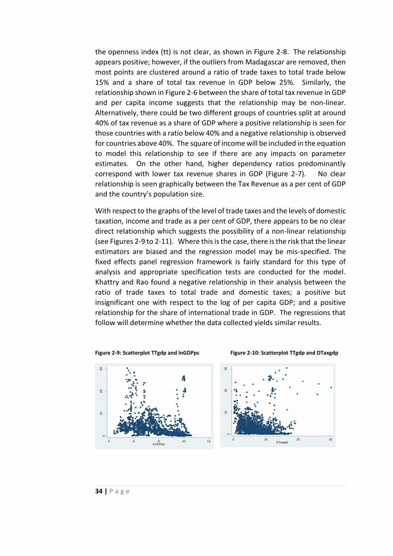
34 | P a g e

the openness index (tt) is not clear, as shown in Figure 2-8. The relationship

appears positive; however, if the outliers from Madagascar are removed, then

most points are clustered around a ratio of trade taxes to total trade below

15% and a share of total tax revenue in GDP below 25%. Similarly, the

relationship shown in Figure 2-6 between the share of total tax revenue in GDP

and per capita income suggests that the relationship may be non-linear.

Alternatively, there could be two different groups of countries split at around

40% of tax revenue as a share of GDP where a positive relationship is seen for

those countries with a ratio below 40% and a negative relationship is observed

for countries above 40%. The square of income will be included in the equation

to model this relationship to see if there are any impacts on parameter

estimates. On the other hand, higher dependency ratios predominantly

correspond with lower tax revenue shares in GDP (Figure 2-7). No clear

relationship is seen graphically between the Tax Revenue as a per cent of GDP

and the country’s population size.

With respect to the graphs of the level of trade taxes and the levels of domestic

taxation, income and trade as a per cent of GDP, there appears to be no clear

direct relationship which suggests the possibility of a non-linear relationship

(see Figures 2-9 to 2-11). Where this is the case, there is the risk that the linear

estimators are biased and the regression model may be mis-specified. The

fixed effects panel regression framework is fairly standard for this type of

analysis and appropriate specification tests are conducted for the model.

Khattry and Rao found a negative relationship in their analysis between the

ratio of trade taxes to total trade and domestic taxes; a positive but

insignificant one with respect to the log of per capita GDP; and a positive

relationship for the share of international trade in GDP. The regressions that

follow will determine whether the data collected yields similar results.

Figure 2-9: Scatterplot TTgdp and lnGDPpc Figure 2-10: Scatterplot TTgdp and DTaxgdp

01

02

03

0

TT

gd

p

0 10 20 30DTaxgdp

01

02

03

0

TT

gd

p

4 6 8 10 12lnGDPpc

35 | P a g e

Figure 2-11: Scatterplot TTgdp and Trade

Correlation

With respect to Equation 1, Tax Revenue as a percentage of GDP is negatively

correlated with population size, the dependency ratio, and the openness

index. It is strongly and positively correlated with per capita GDP and the level

of urbanisation.

With respect to equation 2, there is small negative correlation between Taxes

on International Trade as a percent of GDP (TTgdp), and the share of domestic

taxes in GDP and the exchange rate. Larger negative correlations are observed

for population size, per capita GDP, and the level of urbanisation.

Unsurprisingly, there is large positive correlation between TTgdp and the

openness index as the numerator is the same in both measures. There is much

smaller correlation between TTgdp, and Trade as a percent of GDP and the

dependency ratio (see Appendix 2B).

2.4 Methodology

Based on the empirical approaches discussed in the Literature Review, this

section uses various methods to analyse the revenue effects of trade

liberalisation and notes the extent to which the results obtained are similar or

different to earlier findings.

The regression model uses a similar panel regression analysis to Khattry and

Rao (2002) in the first instance. The model is then varied by utilising

alternative specifications. The openness index is dropped and the traditional

indicator of openness – trade as a share of GDP – is incorporated into the

model. The time period of the model is also extended from 1972-1998 to

01

02

03

0

TT

gd

p

0 100 200 300 400 500Trade

36 | P a g e

1972-2006. Dummy variables are used for individual countries and years to

capture unobservable country and time specific factors.

2.4.1 Regression Model

The model for the determinants of Total Revenue as a Share of GDP is :

TRgdpit = a0 + a1 lnpopit + a2 ln GDPpcit + a3depit + a4urbpopit + a5ttit + γFE +

δFE + eit (1)

where

TRgdpit is the share of tax revenue in GDP

lnpopit is the natural log of population size

ln GDPpcit is the natural log of per capita GDP

depit is the age-dependency ratio

urbpopit is the degree of urbanisation

ttit is the index of openness, measured by the ratio of international

trade taxes to the volume of total trade. A fall in this ratio is

indicative of greater trade openness.

γFE is the country fixed effect

δFE is the time fixed effect

The model for the determinants of Total Trade Tax as a share of GDP is as

follows:

TTgdpit = a0 + a1 ttit + a2 ttit2+ a3ERit + a4 lnpopit + a5 ln GDPpcit + a6depit +

a7urbpopit + a8tradeit + a9Dtaxgdpit + γFE + δFE + eit (2)

where

TTgdpit is the share of trade tax revenue in GDP

ttit is the index of openness, measured by the ratio of international

trade taxes to the volume of total trade. A fall in this ratio is

indicative of greater trade openness.

ERit is the nominal exchange rate

lnpopit is the natural log of population size

37 | P a g e

ln GDPpcit is the natural log of per capita GDP

depit is the age-dependency ratio

urbpopit is the degree of urbanisation

tradeit is trade as % of GDP

Dtaxgdpit is domestic taxes on goods and services as % of GDP

γFE is the country fixed effect

δFE is the time fixed effect

It should be noted that Equation 2 in particular has endogeneity issues as,

arguably, it is likely that the error term is not uncorrelated with the

independent variable Taxes on International Trade as a percent of Total Trade

(tt). Changes in Trade as a share of GDP may influence directly the ratio “tt”.

2.4.2 Regression Results

Using a fixed effects regression technique, regressions were run for equations

1 and 2 – both for the time period 1972-1998 to compare to Khattry and Rao’s

(2002) results and for the extended time period 1972-2006. Table 2-2 reports

the results and shows that all variables, with the exception of the dependency

ratio, were significant in Equation 1 for both time periods. For the extended

time period, a negative but insignificant relationship is estimated between Tax

Revenue as a per cent of GDP and the dependency ratio. However, for the

reduced time period, a positive but insignificant relationship is observed.

Positive relationships are seen between the share of tax revenue and the level

of urbanization, per capita income, and the index of openness.

As can be seen from Table 2-3, with the exception of the population size

variable and the coefficient on the dependency ratio for the reduced time

period, all signs of coefficients are similar to those obtained by Khattry and Rao

(2002). The difference may be attributed to the slightly smaller sample size in

the equations that were run for the time period 1972-1998. For equation 1,

with TRgdp as the dependent variable, the countries missing were Barbados,

Israel, Myanmar, Paraguay and Singapore.

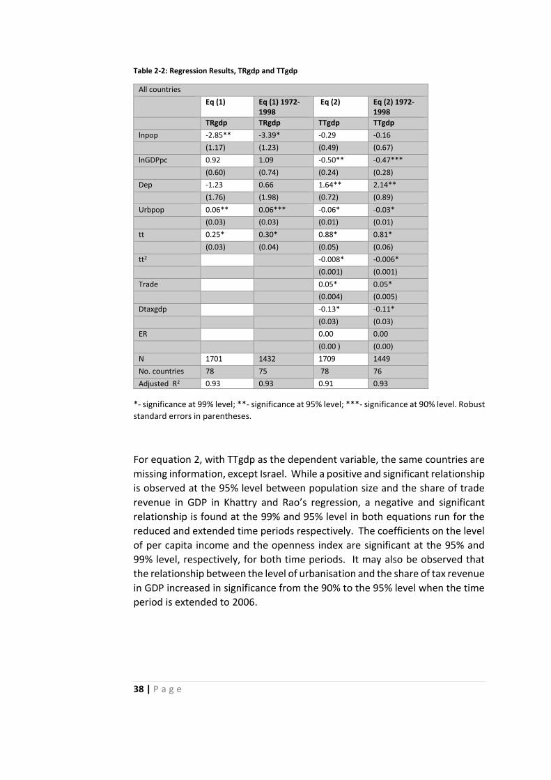
38 | P a g e

Table 2-2: Regression Results, TRgdp and TTgdp

All countries

Eq (1) Eq (1) 1972-1998

Eq (2) Eq (2) 1972-1998

TRgdp TRgdp TTgdp TTgdp

lnpop -2.85** -3.39* -0.29 -0.16

(1.17) (1.23) (0.49) (0.67)

lnGDPpc 0.92 1.09 -0.50** -0.47***

(0.60) (0.74) (0.24) (0.28)

Dep -1.23 0.66 1.64** 2.14**

(1.76) (1.98) (0.72) (0.89)

Urbpop 0.06** 0.06*** -0.06* -0.03*

(0.03) (0.03) (0.01) (0.01)

tt 0.25* 0.30* 0.88* 0.81*

(0.03) (0.04) (0.05) (0.06)

tt2 -0.008* -0.006*

(0.001) (0.001)

Trade 0.05* 0.05*

(0.004) (0.005)

Dtaxgdp -0.13* -0.11*

(0.03) (0.03)

ER 0.00 0.00

(0.00 ) (0.00)

N 1701 1432 1709 1449

No. countries 78 75 78 76

Adjusted R2 0.93 0.93 0.91 0.93

*- significance at 99% level; **- significance at 95% level; ***- significance at 90% level. Robust

standard errors in parentheses.

For equation 2, with TTgdp as the dependent variable, the same countries are

missing information, except Israel. While a positive and significant relationship

is observed at the 95% level between population size and the share of trade

revenue in GDP in Khattry and Rao’s regression, a negative and significant

relationship is found at the 99% and 95% level in both equations run for the

reduced and extended time periods respectively. The coefficients on the level

of per capita income and the openness index are significant at the 95% and

99% level, respectively, for both time periods. It may also be observed that

the relationship between the level of urbanisation and the share of tax revenue

in GDP increased in significance from the 90% to the 95% level when the time

period is extended to 2006.

39 | P a g e

Table 2-3: Comparison of Khattry and Rao Equation 1 Coefficients with Eq. 1 Regression Estimates,

TRgdp

Variables Khattry & Rao Coefficients

Regression Coefficients 1972-1998

Regression Coefficients 1972-2006

lnpopit +** -* -**

ln GDPpcit + +** +**

depit - + -

urbpopit +* +*** +**

ttit +* +* +*

*- significance at 99% level; **- significance at 95% level; ***-significance at 90% level.

With respect to Equation 2, which has the share of trade taxes in GDP as the

dependent variable, when the similar time frame (1972-1998) is applied,

domestic taxes as a per cent of GDP has a negative and significant relationship

with the share of taxes on international trade in GDP. (See Tables 2-3 and 2-4

for a comparison of regression coefficients.) This concurs with the significant

negative relationship that Khattry and Rao estimate in their model and this is

also found in the extended model. In addition, the level of urbanisation was

estimated to have a significant negative relationship with Taxes on

International Trade over the period 1972-1998. Khattry and Rao (2002) found

a negative but insignificant relationship for this variable. A positive and

significant relationship was found between TTgdp and the dependency ratio at

the 95% level of significance for both time periods. The exchange rate variable

(ER) was not found to be significant for both time frames.

Table 2-4: Comparison of Khattry and Rao Equation 2 (TTgdp) Coefficients with Regression Results

Variables Khattry and Rao Coefficients

Regression Coefficients 1972-1998

Regression Coefficients 1972-2006

ttit +* +* +*

ttit2 -* -* -*

ERit + + +

lnpopit +* - -

ln GDPpcit + -*** -**

depit + +** +**

urbpopit - -* -*

tradeit +* +* +*

Dtaxgdpit -* -* -*

*- significance at 99% level; **- significance at 95% level; ***-significance at 90% level

40 | P a g e

While Khattry and Rao (2002) found a positive but insignificant relationship

between GDP per capita and total trade taxes as a share of GDP, the regression

coefficient for this variable for both time periods was found to be negative and

significant; that is, as per capita income increases, one is likely to observe a

decrease in the proportion of international trade taxes in GDP. This result is

consistent with economic theory and observed patterns discussed in Section

2.3.2 where countries with higher levels of income tend to have lower

proportion of trade tax revenue in GDP due to diversification of sources of

taxation and other factors. Additionally, a negative and insignificant

relationship was found between population size and taxes on international

trade. This result was inconsistent with the positive and significant

relationship found by Khattry and Rao (2002). This may be explained by the

different samples used. Barbados, Israel, Myanmar, Paraguay and Singapore

are missing from the model run for 1972-1998 when compared to Khattry and

Rao’s sample.

2.4.3 Specification Tests

The Hausman test was conducted on both Equations 1 and 2 to see if a random

effects estimator would be more appropriate than a fixed effects estimator.

The results of the test on Equation 2 show that the coefficients estimated by

the efficient random effects estimator are not the same as the ones estimated

by the consistent fixed effects estimator. In this case, it is best to use a fixed

effects model. The test could not be performed on Equation 1 as the data

failed to meet the asymptotic assumptions of the test.

The Wooldridge test for serial autocorrelation in panel data sets revealed that

both equations have serial autocorrelation. Heteroskedasticity is also present

in both equations and so, robust standard errors are reported for the models.

In addition, tests were conducted for non-linearity in the per capita income

variable. As shown in Figure 2-12, the predicted values of the natural log of

per capita income (lnGDPpc) in the model are different from the lowess

smoothing curve estimate. This suggests that that the relationship is likely to

be non-linear. Equations were estimated including the square of per capita

income, with results reported in Table 2-5. The square term of per capita GDP

is significant in all equations. However, as all the values of the remaining

parameters are similar in direction and significance as those observed in

models without the squared term, it is clear that the linear estimator does not

significantly bias the results. The next section examines the differing effects of

the model if countries are grouped by income.

41 | P a g e

Figure 2-12: Augmented Component Plus Residual Plot for lnGDPpc, Equation 1

Table 2-5: Regression Results with the square of Per capita GDP, TRgdp and TTgdp

All countries

Eq (1) Eq (1) 1972-1998

Eq (2) Eq (2) 1972-1998

TRgdp TRgdp TTgdp TTgdp

lnpop -5.95* -6.92* -3.27* -2.02*

(1.43) (1.54) (0.60) (0.75)

lnGDPpc 9.96* 12.47* 9.04* 5.81*

(2.81) (3.57) (1.26) (1.49)

lnGDPpc2 -0.65* -0.82* -0.67* -0.44*

(0.19) (0.24) (0.08) (0.10)

Dep -0.78 0.54 2.20* 2.21**

(1.76) (1.96) (0.71) (0.87)

Urbpop 0.10* 0.10* -0.03* -0.01

(0.03) (0.04) (0.01) (0.01)

tt 0.26* 0.31* 0.90* 0.81*

(0.04) (0.04) (0.05) (0.06)

tt2 -0.008* -0.006*

(0.001) (0.001)

Trade 0.05* 0.05*

(0.004) (0.005)

Dtaxgdp -0.13* -0.10*

(0.03) (0.03)

ER 0.00 0.00

(0.00) (0.00)

N 1701 1432 1709 1449

No. countries 78 75 78 76

Adjusted R2 0.93 0.93 0.92 0.93

*- significance at 99% level; **- significance at 95% level; ***-significance at 90% level. Robust

standard errors in parentheses.

35

40

45

50

55

60

Aug

men

ted c

om

pon

ent p

lus r

esid

ua

l

4 6 8 10lnGDPpc

Residuals Linear prediction

Lowess smooth

42 | P a g e

2.4.4 Breakdown by Country Group

There are likely to be differences in the relationships between the dependent

and independent variables for individual country groups – low income, lower

middle income, upper middle income and high income. Tables 2-6 and 2-7

show the results of regression run for Equations 1 and 2 respectively for each

country grouping. For Equation 1, the openness index and the level of

urbanization are the only variables that exhibit a consistent (positive)

relationship with the share of tax revenue in GDP across country groups. With

respect to the openness index, the relationship is not significant for the high

income group. In contrast, the level of urbanisation is found to be a significant

variable for only the low income group. Country size, as indicated by total

population, has a positive relationship with TRgdp that is significant for low

income countries. At the same time, a negative relationship is observed for

the three other categories of countries, with the lower middle income and high

income categories showing a significant relationship at the 90% and 99% level,

respectively, between population size and the share of trade revenue in GDP.

Table 2-6: Equation 1 Regression by Country Group, TRgdp

Eq (1) TRgdp 1972-2006

Low Income Lower Middle Income

Upper Middle Income

High Income

lnpop 17.20* -5.42*** -0.87 -0.75*

(2.62) (3.08) (4.75) (2.57)

lnGDPpc 5.53* 1.80*** -0.19 -3.99*

(0.84) (1.03) (1.26) (1.32)

Dep 11.01* -6.09 -11.16** -17.35*

(2.42) (3.98) (5.12) (4.27)

Urbpop 0.39* 0.08 0.09 0.03

(0.08) (0.05) (0.09) (0.05)

tt 0.22* 0.92* 0.27** 0.03

(0.04) (0.08) (0.13) (0.03)

N 390 490 274 547

No. of countries 18 21 12 27

Adjusted R2 0.90 0.80 0.61 0.93

*- significance at 99% level; **- significance at 95% level; ***- significance at 90% level.

Robust standard errors in parentheses.

The relationship between GDP per capita and TRgdp is positive and significant

for low income and lower middle income countries but negative for upper

middle income and high income countries, with significance being observed

only in the case of the latter group. The dependency ratio shows a negative

and significant relationship for upper middle income, and high income groups.

43 | P a g e

A negative relationship is also seen for lower middle income countries but this

is not significant. On the other hand, a significant positive relationship is seen

for low income countries.

With respect to Equation 2 which seeks to quantify the relationship between

Taxes on international trade as a share of GDP (TTgdp) and variables such as

population size, per capita GDP, and Trade as a per cent of GDP (Table 2-7), the

variations across income groups observed for equation 1 are also seen.

Population size has a positive and insignificant relationship with the share of

trade taxes in GDP for low income and high income countries; while the

relationship is negative for lower middle income and upper middle income

countries. Significance is only observed for the upper middle income category.

Table 2-7: Equation 2 Regression by Country Group, TTgdp

Eq (2) TTgdp 1972-2006

Low Income Lower Middle Income

Upper Middle Income

High Income

lnpop 0.25 -0.66 -5.49* 0.27

(1.35) (0.99) (1.36) (1.14)

lnGDPpc 0.16 -0.37 -2.85* -1.09*

(0.40) (0.32) (0.52) (0.39)

Dep 0.66 -2.53** -3.45** -0.43

(1.08) (1.02) (1.34) (1.97)

Urbpop -0.10* -0.03 0.01 -0.03***

(0.03) (0.02) (0.03) (0.02)

tt 0.40* 0.88* 0.51* 1.56*

(0.03) (0.10) (0.11) (0.06)

tt2 -0.003* -0.005 -0.003 -0.02*

(0.0008) (0.005) (0.008) (0.002)

Trade 0.08* 0.06* 0.01* 0.04*

(0.008) (0.006) (0.004) (0.006)

Dtaxgdp -0.17* -0.14* -0.06 -0.09*

(0.06) (0.03) (0.05) (0.03)

ER 0.00** 0.00* 0.00 0.00

(0.00) (0.00) (0.00) (0.00)

N 396 467 274 572

No. of countries 18 21 12 27

Adjusted R2 0.95 0.95 0.94 0.97

*- significance at 99% level; **- significance at 95% level; ***- significance at 90% level. Robust

standard errors in parentheses.

With respect to GDP per capita, lower middle, upper middle and high income

country groups show a negative, but significant only for the last two categories,

relationship with TTgdp. A positive relationship and insignificant relationship

is observed for the low income group.

The dependency ratio varies inversely with the level of international trade

taxes for lower middle income, upper middle income and high income

44 | P a g e

(insignificant) countries. For low income countries, the relationship seen is

positive and insignificant.

The level of urbanisation is shown to have a negative relationship with the level

of international trade taxes for low, lower middle and high income country

groups, with significance at the 99% level for the low income countries and at

the 90% level for high income countries; the relationship is not significant for

lower middle income and high income countries. For the upper middle income

group, the relationship observed is positive but insignificant.

The coefficients on the openness index and trade as a percentage of GDP are

positive and significant at the 99% level for all country groups. This implies

that regardless of the level of development, increases in exports plus imports

as a per cent of GDP generally imply an increase in the level of international

trade taxes as a per cent of GDP. However, an increase in the openness index,

“tt”, means that there is a higher ratio of trade tax revenue to total trade.

Therefore as “tt” increases, the economy becomes less open), the positive

coefficient on the openness index suggests that international trade tax as a

percent of GDP is likely to rise as an economy becomes less open.

Domestic taxes as a per cent of GDP have a negative and significant

relationship with TTgdp for low, lower middle, and high income countries. A

negative but insignificant relationship is observed for upper middle income

countries. Although the estimated coefficient is very small, the Exchange Rate

variable is significant for low income and lower middle income countries, at

the 95% and 99% level respectively, but insignificant for upper middle income

and high income countries.

Table 2-8 shows the results of running both equations for only developing

countries, that is, countries in the high income category were left out. These

regressions yield results that are generally similar to those obtained by Khattry

and Rao (2002) for both models. However, there is now a positive relationship

between population size and the share of international trade tax revenue as a

percentage of GDP (TTgdp). All other signs remain unchanged. With respect

to the Total Revenue equation (TRgdp), the coefficients on the population size

and dependency variables have changed to positive, with the other signs

remaining unchanged.

45 | P a g e

Table 2-8: Regressions without high income countries, TRgdp and TTgdp

Eq (1) Eq (1) 1972-1998

Eq (2) Eq (2) 1972-1998

TRgdp TRgdp TTgdp TTgdp

lnpop 4.45* 5.51* 0.94 1.13***

(1.70) (2.04) (0.60) (0.68)

lnGDPpc 1.87* 2.86* -0.84* -0.72**

(0.67) (0.81) (0.27) (0.28)

Dep 0.02 2.53 2.24* 1.76**

(1.99) (2.15) (0.67) (0.81)

Urbpop 0.04 0.02 -0.06* -0.05*

(0.04) (0.05) (0.01) (0.01)

tt 0.35* 0.42* 0.58* 0.59*

(0.05) (0.05) (0.04) (0.04)

tt2 -0.005* -0.004*

(0.0009) (0.0008)

Trade 0.04* 0.05*

(0.005) (0.005)

Dtaxgdp -0.12* -0.11*

(0.03) (0.03)

ER 0.00 0.00***

(0.00 ) (0.00)

N 1154 966 1137 958

No. of countries 51 50 51 50

Adjusted R2 0.81 0.82 0.92 0.93

*- significance at 99% level; **- significance at 95% level; ***- significance at 90% level. Robust

standard errors in parentheses.

These models have examined fully the effects of liberalisation using the fixed

effects model of Khattry and Rao (2002). It has been shown that this model is

robust to changes in time periods and has varying effects depending on the

country group under study. One consistent finding across all models is that

the openness index has a positive relationship with both Total Tax Revenue

and Trade Tax Revenue as a share of GDP. Due to its construction, an increase

in the index means that the economy is becoming less open and therefore the

results in this case suggest that as an economy becomes less open, trade tax

revenue and total tax revenue as a share of GDP increases. This finding will be

further examined given the challenges with using the openness index (tt) and

the next section will present alternative measures that could be used, such as

the traditional indicator of openness – trade as a per cent of GDP, and event

analysis.

46 | P a g e

2.5 Addressing Endogeneity in the Model

Khattry and Rao (2002) use “tt” as a new measure of openness. This variable

is the ratio between total international trade taxes and total trade. For them,

a decrease in this ratio means greater openness. This indicator has certain

challenges with respect to measuring the concept of openness. In the first

instance, Khattry and Rao themselves note that there is the potential criticism

that this measure is endogenous with respect to the dependent variable (total

trade taxes as a share of GDP). They note the potential solutions such as using

instrumental variables (Lee (1993); Frankel and Romer (1999)) but find that

findings from these studies are not superior to measures that use tariffs

directly. This criticism could be avoided by using the traditional indicator of

openness – trade as a percentage of GDP – in their models.

They also note other potential shortcomings of using this “index of openness”,

including possible underestimation of the Laffer effect of peak tariffs and of

the impact of smuggling and other tax evasion efforts. Specifically, the

composition of the indicator with total trade as the denominator and taxes on

international trade as the numerator does not adequately capture cases where

there may be a reduction in the tariff that leads to an increase in international

trade tax revenue. This would result in an increase in the openness index, “tt”,

ceteris paribus. However, the economy in this case did not become less open.

Khattry and Rao (2002) counter this criticism by arguing that changes in trade

volume (the denominator) reflect the net effect of policy changes and

exogenous factors and therefore, the index accommodates instances such as

these. This argument should be rejected as the relative effect depends on the

extent to which there has been an increase in marginal trade tax revenue vis-

á-vis total trade. Agbeyegbe et al. (2006) also point out that this measure is

limited in its application as a close relationship is not directly observed

between changes in exports and trade liberalisation.

Greenaway and Milner (1991) note that the net effect of a tariff reduction is

dependent on the initial tariff and the elasticity of demand for imports over

the tariff range in question. Trade tax revenue will increase if the initial tariff

is above the revenue maximising rate. They also note external effects of

liberalisation such as reducing the incentive for smuggling thereby increasing

compliance and the tax base. A reduction in trade tax revenue would result if

the initial tariff is below the revenue maximizing rate. For Greenaway and

Milner (1991), the net effect of tariff liberalisation is dependent on the location

of existing rates in relation to the revenue maximising rate, the shares of the

respective imports in total imports, and relevant individual own and cross price

elasticities of demand and supply – a very complex issue.

47 | P a g e

2.5.1 Trade as a share of GDP as the indicator of openness

In order to test its usefulness and to address the problem of endogeneity,

Equations 1 and 2 were run for both time periods excluding the openness

index, “tt”, and using the one-year lag of Trade as a per cent of GDP. Trade as

a share of GDP itself could be seen as being endogenous to the model as it is

also dependent on changes in GDP along with the dependent variables –

international trade taxes (TTgdp) and total tax revenue (TRgdp) as shares of

GDP. Lagging the variable removes the contemporaneous relationship among

the variables and is one way to address this issue. In addition to the one-year

lag, regressions were also run with the three-year lag of Trade as a share of

GDP to test for sensitivity of the time period chosen.

Table 2-9: Regressions using 1-year lag of Trade, TRgdp and TTgdp

All countries

Eq. 1 (1972-2006)

Eq. 1 (1972-1998)

Eq. 2 (1972-2006)

Eq. 2 (1972-1998)

TRgdp TRgdp TTgdp TTgdp

lnpop -9.16* -8.25* -5.68* -2.44

(1.02) (1.12) (1.06) (1.56)

lnGDPpc -0.92 -0.42 -2.82* -2.16*

(0.58) (0.73) (0.35) (0.40)

Dep -2.37 -0.43 3.91* 1.97

(1.68) (1.99) (1.16) (1.44)

Urbpop 0.08* 0.05 -0.02 -0.01

(0.03) (0.03) (0.02) (0.02)

Tradet-1 0.02* 0.03* 0.03* 0.02*

(0.01) (0.01) (0.01) (0.01)

Dtaxgdp -0.29* -0.27*

(0.04) (0.05)

ER 0.00* 0.00

(0.00) (0.00)

N 2077 1681 1713 1447

No. of countries

78 76 78 76

Adjusted R2

0.93 0.93 0.74 0.76

*- significance at 99% level; **- significance at 95% level; ***- significance at 90% level. Robust

standard errors in parentheses.

With respect to Equation 1 with Tax Revenue as a percentage of GDP as the

dependent variable, the Adjusted R-squared value remains high for the

equation without “tt” at 0.93 (see Table 2-9). This suggests that the model

does not lose much of its explanatory power if “tt” is dropped and replaced by

Trade. The one-year lag of Trade as a share of GDP is shown to have a positive

and significant relationship (at the 99% level) with the Tax Revenue as a per

48 | P a g e

cent of GDP. A negative and significant relationship is found between the

share of tax revenue and population size; while a positive and significant

relationship is found with respect to the level of urbanisation (at the 99% level

of significance). The dependency ratio and the level of per capita income have

negative but insignificant relationships with the share of tax revenue in GDP.

When the reduced time period is applied to the equation, population size

remains a significant variable in the model and the level of urbanisation is no

longer a significant variable.

For the extended time period with the one-year lag of Trade as a share of GDP

(Tradet-1) as the only indicator of openness in Equation 2, significant negative

relationships were found between the share of Taxes on International Trade in

GDP and population size, the level of per capita income, and the share of

domestic taxes on GDP – all at the 99% level. Significant positive relationships

were found with respect to the dependency ratio, and Trade as a per cent of

GDP. Hence, by this estimate, higher trade means higher taxes on

international trade, ceteris paribus. Additionally, when the time period is

reduced, two variables lose their significance: population size, and the

dependency ratio. The exchange rate is not significant in either time period.

The adjusted R-squared falls substantially in the model without “tt”, however.

This is not surprising, given the significant correlation between TTgdp and “tt”

because of the inclusion of the value of taxes on international trade as an

element in both variables.

Another variation of the model in Equation 2 was undertaken by excluding the

one-year lag of Trade as a per cent of GDP as an independent variable. Thus,

“tt” and its square was the only indicator of openness. The results are reported

in Table 2-10 and are different from those obtained in earlier estimates with

respect to the fact that in this estimation, population size, the level of per

capita income, and the dependency ratio do not have a significant relationship

with the share of international trade taxes in total trade. The significant

variables for both time periods are the level of urbanisation, the openness

index and its square, the share of domestic taxes in GDP, and the exchange

rate variable.

It should be noted that the removal of the openness variable has a greater

impact on Equation 2 than on Equation 1. This is expected given the high

degree of correlation between the dependent variable (TTgdp) and the

openness index (tt) and the endogeneity issues associated therewith.

Importantly, the revised regressions with the one-year lag of the traditional

indicator of openness (Trade as a share of GDP) indicate that an increase in

international trade increases trade tax revenue and total tax revenue. This is

contrary to Khattry and Rao’s (2002) finding that an increase in openness

49 | P a g e

negatively affects trade tax revenue and total tax revenue. The digression

suggests that the tt openness index may not be an adequate indicator to

capture the effects of liberalisation on tax revenue.

Table 2-10: Equation 2 without Trade, TTgdp

1972-2006 1972-1998

TTgdp TTgdp

lnpop -0.62 -0.21

(0.55) (0.73)

lnGDPpc -0.07 0.001

(0.27) (0.32)

Dep 1.14 1.30

(0.78) (0.98)

Urbpop -0.04* -0.03**

(0.01) (0.01)

tt 0.85* 0.76*

(0.05) (0.06)

tt2 -0.007* -0.005*

(0.001) (0.001)

Trade ------ ------

Dtaxgdp -0.15* -0.10*

(0.03) (0.03)

ER 0.00* 0.00**

(0.00) (0.00)

N 1709 1449

Adjusted R2 0.89 0.91

*- significance at 99% level; **- significance at 95% level; ***- significance at 90% level. Robust

standard errors in parentheses.

In addition, the findings are sensitive to the lag chosen for Trade as a share of

GDP (see Table 2-11). The three-year lag of Trade as a share of GDP is

significant at the 95% level for Equation 1, with TRgdp as the dependent

variable, over the period 1972-2006. However, income as measured by GDP

per capita and the dependency ratio are now significant variables. The results

for the reduced time period (1972-1998) are not sensitive to a change in the

lag of trade as a share of GDP as the results remain the same. Only population

size and the three-year lag of Trade as share of GDP are significant for this time

period.

With respect to Equation 2, with TTgdp as the dependent variable, the results

are not sensitive to a change in lag value of Trade as a share of GDP to three

years. Population size, per capita income, the dependency ratio, domestic

taxes as a share of GDP and the exchange rate all remain as significant variables

with similar directional relationships as the equation with the one-year lag of

Trade as a share of GDP. The results are the same when the time period is

reduced to 1972-1998.

50 | P a g e

Table 2-11: Regressions using 3-year lag of Trade, TRgdp and TTgdp

All countries

Eq. 1 (1972-2006)

Eq. 1 (1972-1998)

Eq. 2 (1972-2006)

Eq. 2 (1972-1998)

TRgdp TRgdp TTgdp TTgdp

lnpop -9.48* -8.78* -6.66* -3.53**

(1.05) (1.19) (1.13) (1.70)

lnGDPpc -1.09**** -0.79 -2.89* -2.01*

(0.60) (0.76) (0.39) (0.45)

Dep -3.25*** -2.03 3.68* 1.40

(1.70) (2.03) (1.20) (1.55)

Urbpop 0.08* 0.04 -0.03 -0.02

(0.03) (0.03) (0.02) (0.02)

Tradet-3 0.02** 0.03* 0.02* 0.004

(0.008) (0.01) (0.01) (0.006)

Dtaxgdp -0.30* -0.27*

(0.04) (0.05)

ER 0.00* 0.00**

(0.00) (0.00)

N 2022 1618 1659 1389

No. of countries

78 76 78 76

Adjusted R2

0.93 0.94 0.73 0.76

*- significance at 99% level; **- significance at 95% level; ***- significance at 90% level. Robust

standard errors in parentheses.

The next chapter will apply one other method - event analysis - to the question

of the impact of liberalisation on taxes on tax revenue. This will assist in

evaluating the validity of findings of these models.

2.6 Conclusions

This chapter has examined two techniques to analyse the fiscal implications of

trade liberalisation. Both are set in a fixed effects panel regression model –

the difference lies in the measurement of tariff liberalisation (openness). In

the first instance, equations 1 and 2, with dependent variables as tax revenue

as a share of GDP and international trade tax revenue as a share of GDP,

respectively, were run for two time periods (1972-1998 and 1972-2006). The

results suggest a negative relationship between trade liberalisation, as

measured by the openness index, and international trade tax and total tax

revenue. All variables, but for the dependency ratio, are significant in Equation

1 for both time periods. With the exception of the population size variable and

the coefficient on the dependency ratio for the reduced time period, all signs

of coefficients are similar to those obtained by Khattry and Rao (2002). The

results suggest that the share of tax revenue in GDP increases with advances

in level of urbanization, per capita income, and a fall in an economy’s openness

51 | P a g e

(an increase in the openness index means an economy is becoming less open).

On the other hand, in contrast to Khattry and Rao’s (2002) finding, the

regression results indicate that the share of tax revenue in GDP is likely to fall

as population size increases. With respect to Equation 2, the results show

that the share of international trade tax revenue in GDP is likely to fall as

domestic taxes as a per cent of GDP, and the level of urbanisation increases.

Additionally, it is observed that as per capita income, and the age-dependency

ratio increase, one is likely to observe an increase in the proportion of

international trade taxes in GDP.

In order to determine any variations due to differing levels of development,

these models were then analysed by country group. The results show that

the share of tax revenue in GDP is likely to fall as an economy becomes more

open. For Equation 1, the openness index is one of two variables (the other

being the level of urbanisation) that exhibit a consistent (positive) relationship

with the share of tax revenue in GDP across country groups. Importantly, the

results suggest that international trade tax revenue tends to fall over time as

a country develops (level of per capita income increases). For equation 2, the

coefficients on the openness index and trade as a percentage of GDP are

positive and significant for all country groups. The positive coefficient on trade

as a percentage of GDP implies that regardless of the level of development,

increases in exports plus imports as a per cent of GDP generally imply an

increase in the level of international trade taxes as a per cent of GDP.

However, in contrast, as an increase in the openness index means that an

economy is becoming less open, the positive coefficient on the openness index

suggests that international trade tax as a percent of GDP is likely to rise as an

economy becomes less open. The model also predicts that trade tax revenue

is likely to fall as domestic taxes as a per cent of GDP increase. This relationship

is significant for low, lower middle, and high income countries and suggests

that domestic taxes are one avenue through which countries may recoup lost

trade tax revenue as a result of trade liberalisation.

As both models utilised by Khattry and Rao (2002) contain an openness index

which presents certain challenges, including the potential for endogeneity

within the model, the model was varied to utilise an alternative measure of

openness - trade as a per cent of GDP. It should be noted that Trade as a share

of GDP is also endogenous within the models as the dependent variables are

also conditioned on GDP. The method chosen to address this was to lag Trade

as a share of GDP for one and three-year periods. Choosing two different lags

allowed for testing for robustness of results to the time period chosen. When

the one-year lag of Trade as a percent of GDP is used as the indicator of

openness, the results show a positive relationship between openness, and

trade and total tax revenue as a share of GDP for both equations; that is, trade

52 | P a g e

tax revenue and total tax revenue are likely to increase as an economy

becomes more open. This suggests that the models are sensitive to the

indicator of openness used. In addition, the final effect of trade liberalisation

is difficult to predict and is dependent on a variety of factors that may be

difficult to capture in one model. Except for Equation 1 with total tax revenue

(TRgdp) for the time period, 1972-1998, the results are not sensitive to the lag

value chosen. One can therefore use the one-year lag which provides greater

degrees of freedom and more power to the results.

Given the findings from these models, it is clear that there is much room for

further analysis in this area to find better ways of measuring the net impact of

liberalisation on government revenue. The analysis could be extended to

examine the impact of lowering tariffs as against eliminating non-tariff

barriers, for example. In addition, there could be further breakdown of the

different components of trade taxes, by import taxes and export taxes, for

example, to see how the liberalisation process impacts each component. There

is also room to analyse the net effect of trade liberalisation by using a general

equilibrium model that can take account of the impact of relative prices and

demand for final and intermediate goods as a result of changes in the price

level due to adjustments in the tariff structure.

53 | P a g e

APPENDIX 2A - COUNTRIES IN EQUATIONS 1 AND 2 Low Income Lower Middle Income

Bangladesh Bhutan Burkina Faso Cameroon Burundi Colombia Congo, Dem. Rep. Congo, Rep. Gambia, The Dominican Republic Ghana Ecuador India Egypt, Arab Rep. Kenya Fiji Liberia Guyana Madagascar Jordan Malawi Lesotho Myanmar Morocco Nepal Nicaragua Pakistan Paraguay Papua New Guinea Peru Sierra Leone Philippines Uganda Sri Lanka Zambia Swaziland Zimbabwe Syrian Arab Republic

Thailand

Tunisia

Upper Middle Income High Income Argentina Australia Japan Botswana Austria Korea, Rep.

Brazil Barbados Luxembourg

Chile Belgium Malta Costa Rica Canada Netherlands

Malaysia Cyprus New Zealand

Mauritius Denmark Norway Mexico Finland Portugal Panama France Singapore

South Africa Greece Spain Turkey Iceland Sweden Uruguay Ireland Switzerland

Israel United Kingdom

Italy United States

54 | P a g e

APPENDIX 2B: CORRELATION MATRICES

Table 2-12: Correlation Matrix for Equation 1

TRgdp lnpop lnGDPpc tt Dep Urbpop

TRgdp 1.0000

lnpop -0.1369 1.0000

lnGDPpc 0.6729 -0.0045 1.0000

Tt -0.1332 0.0121 -0.5043 1.0000

Dep -0.4799 -0.1115 -0.7801 0.4047 1.0000

Urbpop 0.5111 0.0258 0.8372 -0.4306 -0.6787 1.0000

Table 2-13: Correlation Matrix for Equation 2

TTgdp lnpop lnGDPpc tt tt2 DTaxgdp Trade ER Dep Urbpop

TTgdp 1.00

lnpop -0.32 1.00

lnGDPpc -0.27 -0.03 1.00

tt 0.72 0.02 -0.47 1.00

tt2 0.52 0.04 -0.21 0.83 1.00

DTaxgdp -0.09 -0.05 0.51 -0.11 0.13 1.00

Trade 0.34 -0.57 0.15 -0.14 -0.09 0.03 1.00

ER -0.04 0.06 0.005 -0.04 -0.01 0.07 -0.01 1.00

Dep 0.28 -0.10 -0.78 0.38 0.16 -0.43 -0.11 -0.04 1.00

Urbpop -0.25 -0.01 0.84 -0.41 -0.20 0.47 0.15 0.02 -0.67 1.00

55 | P a g e

3. EVENTS ANALYSIS OF THE IMPACT OF TRADE LIBERALISATION

3.1 Introduction

The impact of trade reform on fiscal revenue can be measured in various ways

but a key variable to consider is the definition of trade reform itself. Some

models have used the degree of openness as an indicator of trade reform.

Openness indicators include, for example, a change in exports plus imports as

a share of GDP or the openness index (the ratio of total trade tax revenue to

the value of total trade as in Khattry and Rao (2002) and Chapter 2), that

indicate a country’s general orientation towards the world. Researchers utilise

an openness variable to examine the impact of trade reform on fiscal revenue,

taking into account other variables such as population size and the

dependency ratio. The vast majority of these models measure liberalisation

over time although trade liberalisation was often driven by economic shocks

and externally imposed under loan agreements with multilateral lending

institutions. As a condition of the loans, countries (mainly developing) were

required to undergo a series of reforms, including trade liberalisation. In these

cases, trade liberalisation can be linked to specific periods when these reforms

occur.

In this case, one can analyse the impact of trade liberalisation directly by

observing the changes in key variables, such as total tax revenue and trade tax

revenue as a share of GDP, in the period before and after liberalisation. Events

analysis is a valid methodology for conducting this analysis as it takes into

account the context within which reforms occurred and how that may have

affected the composition, pace and sequencing of reforms. This chapter

explores this methodology and applies it to an analysis of the impact of trade

liberalisation on total tax revenue and trade tax revenue as a share of GDP. It

compares the results from these models to those obtained in Chapter 2 in

order to evaluate robustness of findings.

Chapter 3 also explores the issue of heterogeneity within the sample,

specifically relating to the varying levels of development among countries and

the treatment of export taxes by individual countries over the time period and

their impact on the liberalisation experience and fiscal revenue. The fact that

developing countries often undertook trade reforms as part of a lending

programme with the Fund or the World Bank means that their liberalisation

experience is likely to be different from countries that liberalised with no

external impetus. For example, the pace of liberalisation may have been more

aggressive for those countries in a reform programme when compared to

those that liberalised on their own timetable, leaving them vulnerable to

56 | P a g e

shocks to fiscal revenue. This chapter analyses the models in terms of

developing and developed countries in order to explore these issues and to see

if there is any empirical basis for these inferences.

In addition, export taxes constitute a relatively small proportion of total trade

tax revenue for most countries. However, for those countries where export

taxes constitute a large proportion of government revenue, it may be argued

that they may seek to implement a reform programme that aims to minimise

the impact on export tax revenue. In this case, they may therefore be willing

to reduce import taxes at a much faster rate and decrease export taxes more

slowly when compared to countries that do not have a high proportion of

export tax to total trade tax revenue. Moreover, under IMF and World Bank

reform programmes, export taxes were often targeted in the first phase of

reform; thus, putting even more pressure on those countries with significant

export tax revenue levels. In this context, it would be interesting to see if there

are significant differences in fiscal revenue of those countries over time when

compared to other countries.

Chapter 3 starts by providing an overview of the events measures that will be

used in the study. It then goes on to explore the correlation between the

events measures and the fiscal revenue indicators – total tax revenue and

trade tax revenue. The results from the regression models are then analysed.

The next section goes on to explore heterogeneity within the sample based on

the level of income and dependence on export taxes. The chapter then

concludes by summarising the main findings and implications for future work.

3.2 Measuring Events

There are several approaches to measuring events. Some include composite

indices, while others explore specific indicators of a particular event. All of

them involve a subjective assessment, to some extent, of the variables to be

used as an event indicator and the date the event occurred. An events

indicator may be viewed as being exogenous to the model as it is less likely to

be correlated over time with trade and total tax revenue as a share of GDP.

Indeed, for developing countries, liberalisation events occur oftentimes as part

of package of reforms under the International Monetary Fund (IMF) or World

Bank. One may therefore be able to use a dummy variable such as the date

when a country entered into a structural adjustment loan with the World Bank

(Greenaway et al. (2002)). Using indicators related to a specific year or event,

however, may present challenges because liberalisation takes place over time

and there may be years when an economy is perceived to be open but a change

in government or other external factors alter the movement towards

liberalisation. Although these issues are recognized, events analysis is still

57 | P a g e

useful to examine liberalisation through a different lens. This chapter draws

upon the work of Sachs and Warner (1995), Dean et al. (1994), and Greenaway

et al. (2002) to identify the year of liberalisation events and apply the analysis

in an econometric model to assess the impact of these events on government

revenue.

With respect to composite indices, the Sachs-Warner index is one of the most

often cited work in empirical studies. Sachs and Warner (2005) develop a

composite indicator of the degree of openness of thirty-four countries using

five criteria. A country is judged to be closed if it had:

1. Nontariff barriers (NTBs) that apply to 40% or more of its trade.

2. Average tariff rates greater than 40%.

3. A black market exchange rate that deviated from the official exchange rate

by 20% or more, on average, during the 1970s or 1980s.

4. A socialist economic system.

5. A state monopoly on major exports.

The liberalisation date is set from the year at which the economy is deemed to

be continually open until the end of the sample period of the study in 1994.

Sachs and Warner (1995) note that there are limitations to the methodology

used such as the subjective dating of the liberalisation event and the arbitrary

levels of indicator thresholds. In addition, there is the criticism that the Sachs-

Warner index ascribes a discrete value (either liberalisation occurred or it did

not) to a process that usually lasts several years (David (2008)). Other

challenges include the lack of significance and small magnitude of the effect of

tariffs and quotas in the index once all its constituents are separated (Harrison

and Hanson (1999) and Rodriguez and Rodrik (2001). While the index is an

imperfect measure (as are all indicators of openness), it is useful and relevant

as it includes features that are typical of a closed economy and can therefore

be used to compare and contrast the effect of liberalisation with open

economies.

Alternatively, studies such as Dean et al. (1994) evaluate the individual

components of trade reform and therefore, do not face criticism on conflating

several factors in one index as seen in Sachs-Warner (1995). They assess

changes in tariffs, non-tariff barriers, foreign exchange controls, and export

impediments in thirty-two countries from 1982 to 1993 in South and East Asia,

Latin America, and Africa. Data include changes in the level, range, and

dispersion of tariffs, and the extent of quantitative restrictions. Based on the

changes in these variables, a year(s) of liberalisation is derived for each

58 | P a g e

country. As is often the case in studies of this nature, there is some subjectivity

in ascribing the year of reform given that there are several indicators that may

not be all pointing in the same direction at the same time.

There is also the use of a relatively simple policy proxy dummies, such as the

date of signature of a country’s Structural Adjustment Loan with the World

Bank. Measures such as these do not directly measure the liberalisation

experience; however, a structural adjustment loan may be seen as an indicator

of a country’s intent to liberalise (based on the policy conditionalities of the

loan) and thus, provide an indicator that is not directly correlated with trade

tax revenue and total tax revenue. Greenaway et al. (2002) utilise such an

approach in their analysis of liberalisation events.

The event measures are distinct and are not interchangeable as most provide

different estimates of the liberalisation event even for the same countries. In

fact, only Venezuela records the same year of liberalization for all three

measures and another two countries – Ghana and Costa Rica - have a variance

of one year among the event indicators. The analysis in this section treats each

event indicator separately and a judgement is not made on the superiority of

one measure over the other. This approach is useful as it tests the robustness

of these measures across time and may provide an indication of the main

factors that influence trade tax and total tax revenue, in general, as the event

indicators measure liberalisation differently.

Similar to Greenaway et al. (2002), we include two variations of the Dean et al.

and the Sachs-Warner dummies in the regression models – one where the

dummies take a value of 1 only in the year the event occurred and the other

where the dummy takes the value of 1 in the year of liberalisation and for all

subsequent years. The event indicators replace the openness index in both

equations estimated by Khattry and Rao (2002). The model also incorporates

lagged values of the Dean and Sachs-Warner variables. Appendix 3A provides

the list of the predominantly developing countries used in the sample and the

date of liberalisation based on the three event indicators over the period 1972-

2006. The next section analyses the data that will be used in the regression

models.

3.3 Data Analysis

Each event dummy is plotted against total trade tax revenue as a share of GDP

to see if there is any pattern that can be observed. With respect to the World

Bank dummy, there is no clear pattern pre- and post-signature of a World Bank

Structural Adjustment loan agreement (see Figure 3-1). There are several

59 | P a g e

factors that may influence the relationship between a structural adjustment

loan and total trade taxes as a share of GDP. In the first instance, a reform

programme is multi-faceted and the final impact on trade tax revenue and

total tax revenue depends on the execution of the programme and the

response of the economy to reforms. For example, there may be a revenue-

enhancing component in the form of technical assistance in customs

administration and at the same time, there is a requirement to reduce tariff

peaks on luxury items which may have a negative effect on fiscal revenue. At

the same time, where tariff rates are above the revenue maximising rate, a

reduction in rates may lead to increased revenue as consumers are

incentivised to increase consumption. The final effect on trade tax revenue

depends on the interplay of all these and other factors.

Figure 3-1: Scatterplot of Total Trade Tax Revenue as a Share of GDP and the World Bank Dummy

The plot of trade tax revenue in GDP and the first Sachs-Warner dummy (SW1)

shows that there appears to be a greater proportion of points below the 5%

mark after trade liberalisation. The Sachs-Warner dummy in this case takes

the value of 0 before the year of liberalisation and 1 in the year of liberalisation

and all the subsequent years. It measures the average post reform effect of

trade liberalisation on trade tax revenue as a share of GDP. Although the data

points post-liberalisation appear to be lower, it is not clear that total tax

revenue as a share of GDP is significantly different after trade liberalisation.

From Figure 3-2, it can be seen that trade liberalisation generally took place in

the late 1980s and early 1990s.

05

10

15

20

25

TT

gdp

(%

)

1970 1980 1990 2000 2010Year

TTgdp where WB dummy=1 TTgdp where WB dummy=0

Total Trade Tax Revenue as a Share of GDP and the World Bank Dummy

60 | P a g e

Figure 3-2: Scatterplot Total Trade Tax Revenue as a Share of GDP and the Sachs-Warner1 Dummy

For liberalisation to have taken place using the Sachs-Warner measures, there

would be less Nontariff barriers (NTBs), a significant reduction (>20%) in the

black market exchange rate, a move from a socialist to a free market economy,

and a removal of state monopolies on major exports. The extent to which

these measures generate positive effects depends on how they are

implemented and existing economic structures. For example, a removal or

reduction in NTBs could be revenue enhancing if there is a complementary

shift in trade facilitation that encourages imports. Depending on individual

elasticities of demand and supply of imports, one could see increased trade tax

revenue. On the other hand, if NTBs are removed but an anti-import stance

remains, then one is not likely to see any positive effects on trade tax revenue.

In addition, if there were taxes on exports that were previously collected by

the state monopolies and export taxes are removed under trade reform, then

it is likely that there would be a reduction in export taxes, and therefore trade

taxes collected post-reform, all things being equal. Another factor to consider

is the broader macroeconomic environment. If the rate of GDP growth

exceeds that of trade tax revenue, then the share of tax revenue in GDP is likely

to fall over time. The Sachs-Warner index takes into account exchange rate

changes and movement towards a capitalist economy which have direct

impact on the macroeconomy and GDP. One will therefore have to estimate

the regression models to see how these factors affected the countries in the

sample.

Figure 3-3 plots data points where the second Sachs Warner dummy (SW2)

takes a value of 0 in the years before and after trade liberalisation and 1 in the

year of liberalisation itself. This dummy seeks to capture the immediate

impact of trade liberalisation on trade tax revenue and total revenue as a share

05

10

15

20

25

TT

gdp

(%

)

1970 1980 1990 2000 2010Year

TTgdp where SW1=0 TTgdp where SW1=1

Scatterplot Trade Tax Revenue as a Share of GDP and Sachs-Warner1 Dummy

61 | P a g e

of GDP. There is no clear immediate impact of trade liberalisation on the share

of trade tax revenue in GDP. The immediate impact depends on the nature of

the reform programme, including factors such as the timing and sequencing of

reforms. If there are drastic movements in the exchange rate and immediate

implementation of free market reforms, then immediate effects are more

likely to be observed. However, if reforms are implemented over time (as is

likely the case), then significant immediate effects are less likely to be

observed.

Figure 3-3: Scatterplot Total Trade Tax Revenue as a Share of GDP and the Sachs-Warner2 Dummy

Figures 3-4 and 3-5 show a roughly similar picture to the scatterplots of trade

tax revenue in GDP and the Sachs-Warner dummies. The first Dean dummy

(D1) measures the average effect of trade liberalisation on trade tax revenue

and total tax revenue as a share of GDP over time. Figure 3-4 shows that the

share of trade tax revenue in GDP appears to be lower post trade reform. The

Dean measure is based on changes in tariffs, non-tariff barriers, foreign

exchange controls, and export impediments. The average impact of trade

liberalisation on trade tax revenue in GDP therefore depends on the

components of the trade reform, including timing and sequencing

considerations. In addition, one has to take account of the broader economic

reform programme which affects GDP.

05

10

15

20

25

TT

gdp

(%

)

1970 1980 1990 2000 2010Year

TTgdp where SW2=1 TTgdp where SW2=0

Scatterplot Trade Tax Revenue as a Share of GDP and Sachs-Warner2 Dummy

62 | P a g e

Figure 3-4: Scatterplot Total Trade Tax Revenue as a Share of GDP and the Dean1 Dummy

In Figure 3-5, no clear difference is seen between trade tax revenue as a share

of GDP in the year of liberalisation, as measured by the second Dean dummy

(D2), and the years before and after trade reform. Like the SW2 dummy, D2

estimates the immediate impact of trade reform on trade tax revenue as a

share of GDP. The dummy takes a value of 0 in the years before and after trade

reform, and 1 in the year of trade liberalisation. The immediate impact of

trade reform depends on how aggressive is the reform timetable, the nature

of reforms, and the components of the broader economic reform programme,

among other factors.

Figure 3-5: Scatterplot Total Trade Tax Revenue as a Share of GDP and Dean2 Dummy

05

10

15

TT

gdp

(%

)

1970 1980 1990 2000 2010Year

TTgdp where Dean1=1 TTgdp where Dean1=0

Scatterplot Trade Tax Revenue as a Share of GDP and Dean1 Dummy

05

10

15

TT

gdp

(%

)

1970 1980 1990 2000 2010Year

TTgdp where Dean2=1 TTgdp where Dean2=0

Scatterplot Trade Tax Revenue as a Share of GDP and Dean 2 Dummy

63 | P a g e

3.4 Regression Model

This chapter uses an events framework like that employed in Greenaway et al.

(2002) to assess if there is any discernible impact of trade liberalisation on total

tax revenue and trade tax revenue as a share of GDP before and after trade

liberalisation. The three dummy variables used to measure the liberalisation

event are indices developed by Dean et al. (1994), and Sachs and Warner

(1995), and a World Bank dummy which is based on the date that a country

signed a Structural Adjustment Loan (SAL) with the World Bank. The Dean et

al. (1994) measure is based on a subjective assessment of the timing of

liberalisation taking into account changes in tariffs, quotas, export measures,

and exchange rates which assesses when liberalisation occurred in their

sample of thirty-two developing countries. The Sachs and Warner index,

developed for thirty-four countries, assesses whether an economy is open or

closed based upon movements in non-tariff barriers and average tariff levels;

whether or not the country is socialist; the existence of state monopolies over

key exports; and the difference between the official and black market

exchange rates.

These event dummies are included in a model with other independent

variables that are shown to have influence total tax revenue and trade tax

revenue as a share of GDP. These variables include population size, the level

of urbanisation, per capita income and the dependency ratio.

The model explaining Total Revenue as a share of GDP is:

TRgdpit = a0 + a1 lnpopit + a2 ln GDPpcit + a3depit + a4urbpopit + a5Dit + γFE +

δFE + eit (3)

where

TRgdpit is the share of tax revenue in GDP

lnpopit is the natural log of population size

ln GDPpcit is the natural log of per capita GDP

depit is the age-dependency ratio

urbpopit is the degree of urbanisation

Dit is a dummy variable indicating a liberalisation event, either

using the Sachs-Warner (SW), Dean et al. (D), or World Bank

Structural Adjustment Loan (WB) indicator

64 | P a g e

γFE is the fixed effect estimate that captures unobservable country

effects

δFE is the time fixed effect that captures unobservable changes that

occur over time

In addition, the model for Total Trade Tax Revenue as a share of GDP is given

below:

TTgdpit = a0 + a1lnpopit + a2lnGDPpcit + a3depit + a4urbpopit + a5Dit +

a6Dtaxgdpit + a8ERit +γFE + δFE + eit (4)

where

TTgdpit is the share of trade tax revenue in GDP

lnpopit is the natural log of population size

ln GDPpcit is the natural log of per capita GDP

depit is the age-dependency ratio

urbpopit is the degree of urbanisation

Dit is a dummy variable indicating a liberalisation event, either

using the Sachs-Warner (SW), Dean et al. (D), or World Bank

Structural Adjustment Loan (WB) indicator

Dtaxgdpit is domestic taxes on goods and services as % of GDP

ERit is the exchange rate

γFE is the fixed effect estimate that captures unobservable country

effects

δFE is the time fixed effect that captures unobservable changes that

occur over time

The dummy variables in the model take two variations. In the first variation,

the dummies take the value of 0 in the years preceding trade liberalisation and

1 for the year of liberalisation and all subsequent years (SW1, D1, WB1). The

coefficient on these dummy variables therefore captures the average post-

reform effect of trade liberalisation on the share of total tax revenue and trade

tax revenue. The second variation of the dummy variable only takes a value of

1 in the year of liberalisation itself (SW2, D2, WB2), thus capturing the

immediate impact on the share of trade tax and total tax revenue in GDP. The

dummies are also lagged by one and two years to assess if there are any short-

65 | P a g e

term effects on trade tax and total tax revenue related to the liberalisation

event.

Robust standard errors are used as heteroskedasticity is present in both

equations.

A Priori Expectations

There are many competing factors at play that affect the impact of tariff

liberalisation on fiscal revenue, in large part due to the varying forms that trade

reform can be implemented. Reform can comprise the removal of tariffs and

quantitative restrictions up front or over a phased period. Quantitative

restrictions may also be changed to tariffs. Trade reform often comprises

multiple facets that are implemented simultaneously or sequentially. It is

therefore difficult to predict the final impact; however, the analysis of a priori

expectations can be framed in the context of the likely impacts of the measure.

One can predict that the share of trade tax revenue in GDP is likely to have an

inverse relationship with a country’s level of economic development. As a

country becomes more developed, tax systems mature, administrative

experience and efficiencies are gained, and thus other sources of revenue

become much more significant than trade tax revenue. In addition, there may

be greater need for cash transactions and a change in the composition of

imports needed for production as an economy develops leading to a

movement away from trade taxes to domestic import taxes (Greenaway

(1980). As country develops, it is also less likely to be heavily dependent on

primary agricultural products. At the early stages of development, countries

are more likely to impose export taxes on primary products. Under trade

liberalisation, the removal of export taxes is expected to reduce tax yield but

there may be positive effects on tax revenue as other export enhancing

measures such as export credits are implemented as part of the reform

package.

It is also likely that there will be positive revenue effects of tariff liberalisation

if the initial tariff rate is above the revenue maximising rate. In this case, any

reduction of the tariff is likely to increase trade tax revenue as the incentive

for evasion is lessened by the decrease or removal of the tariff and positive

changes in income may be induced. Conversely, if the initial tariff rate is below

the revenue maximising rate, then tariff reduction or elimination is likely to

result in a reduction in government revenue from trade taxes as no positive

changes in income are likely to be induced in this case (Khattry and Rao (2002)).

The net impact of tariff changes will therefore depend on the location of tariffs

relative to the tariff maximising rate, the magnitude of tariff changes, and cross

price elasticities of demand of imports and supply of import substitutes.

66 | P a g e

In addition, the tariff liberalisation programme often simplifies the tariff

structure, reduces the dispersion of tariff rates, and significantly lessens

discretionary tax waivers. Greenaway and Milner (1991) state that this should

be revenue-neutral but there is the potential for positive revenue effects if the

reform induces greater tax compliance. An alternative framework to analyse

this issue is to look at effective rates of protection (Ebrill et al. (1999)). If

reducing tariff dispersion negatively affects effective rates of protection, then

there is likely to be an increase in imports and hence, increased revenue from

trade taxes. In addition, higher tariffs tend to be associated with goods that

have higher price elasticities of demand and if these tariffs are lowered, then

the positive revenue effect is likely to be reinforced through increased demand

for these products.

Another component of trade reform is the replacement of quantitative

restrictions with tariffs, which may have positive revenue effects. The extent

to which this occurs depends on the impact of these tariffs on domestic prices

and hence on domestic demand for the affected products. The change to

tariffs may result in lower consumer prices as supply is no longer restricted,

which may lead to increased demand for the product. Once supply is able to

meet demand, there is likely to be increased revenue from additional imports,

ceteris paribus. As noted by Ebrill et al. (1999), other factors that influence the

final income include the nature of the restriction itself and the administrative

capabilities of the executing agencies of the reform.

Domestic tax revenue is also impacted by trade liberalisation. In many

developing countries, taxes on imported goods and services are an important

source of revenue. Indeed, these taxes are often levied on the tariff-inclusive

price. The removal of tariffs is therefore likely to reduce tax yield if the base is

eroded. Agbeyegbe et al. (2006) note, however, that the ultimate impact on

revenue yield has to take account of possible changes in import demand

(positive) and demand for import substitutes (negative) due to lower prices on

imports from removal of the tariff.

In addition, one often sees some amount of exchange rate adjustment in trade

reform packages. Devaluation is likely to increase the price of imports but the

extent to which this affects customs revenue depends on the price elasticity of

demand for imports. In addition, devaluation makes tradeables more

expensive than non-tradeables. This may have two divergent effects – a

negative impact on customs revenue but a positive impact on domestic

indirect tax revenues. The precise effect depends on the relevant price

elasticity of demand for imports and the price elasticity of supply for import

substitutes. If price elasticity of demand for imports is relatively inelastic then

the government would expect to see increased revenue earnings from tariffs.

67 | P a g e

On the other hand, consumer goods and food items with domestic substitutes

tend to have high elasticity. Currency depreciation also has a positive effect

on exports which may lead to increased revenue from taxes on income. The

net impact therefore depends on these competing considerations (Agbeyegbe

et al. (2006)).

A country’s level of urbanization and age-dependency ratio also may influence

the share of total tax revenue in GDP. In Lewis’ (1954) model of structural

change, an economy becomes more urbanised as it develops. This increases

its revenue need and capacity to tax as the urban population demands

provision of additional public services and provides a focused tax base. In

many developing countries where the rural economy tends to be the dominant

sector, economic activity tends to be less concentrated and mostly informal in

nature, which limits tax administration and collection. Therefore, in some

cases, governments levy taxes on agricultural exports. In addition, the high

age-dependency ratios in many countries mean that the tax base is smaller

than in developed countries which tend to have lower age-dependency ratios.

Finally, the sign on the dummy variable that captures the liberalisation event

can be either positive or negative, depending on the combination of factors

operating during the trade reform process. If there is a positive effect on trade

tax revenue and total tax revenue, one can expect the sign on the dummy

variable coefficient (a5) to be positive, that is, revenue will be higher on

average after the liberalization event relative to the pre-liberalization period.

On the other hand, if trade tax revenue and total tax revenue are adversely

impacted by trade liberalisation, then one can expect a negative sign on a5,

that is, revenue is less on average for the period after liberalisation.

Other impacts of trade liberalisation may also be seen on income and taxes on

profits which are not explicitly explored in these models and may be explored

in a CGE-type setting. Agbeyegbe et al. (2006) note that short-run impacts can

be observed through changes in profits of importers and producers of import

substitutes. Long-run impacts of trade liberalisation may be seen if there are

changes in economic growth and by extension, incomes and income tax

liabilities that may be attributed to the reform programme.

To conclude, it is clear that the final impact of trade reform on fiscal revenue

cannot be predicted with any great degree of certainty. Factors such as the

age dependency ratio, the level of urbanization, and per capita income account

for structural characteristics in the economy that determine a country’s

taxable base. The inclusion of the exchange rate in the trade tax revenue

model accounts for the possible impact of changes in monetary policy on

exports and imports. In addition, there are other factors that influence the

68 | P a g e

final reform outcome, such as the initial tariff structure, price elasticities of

demand and supply for imports and domestic substitutes and the nature of

trade reforms. The next section formally outlines the model that will be used

to analyse the impact of trade liberalisation on fiscal revenue within the

framework of the variables discussed.

Trade as a share of GDP is not included in these models as it likely to be

collinear with the liberalisation event; ceteris paribus, trade liberalisation

should lead to increased trade as a share of GDP.

3.5 Regression Results

Total Tax Revenue as a Share of GDP

The level of urbanisation is shown to have a positive and significant

relationship with total tax revenue as a share of GDP for all models that

measure the average post-reform of effect of trade liberalisation over time

(see Table 3-1). This is consistent with Lewis’ (1954) argument that

urbanisation provides a centralised population for taxation which is easier to

manage than dispersed rural populations. The Sachs-Warner event dummy

itself (SW1) is significant at a 90% level and estimates that the share of total tax

revenue in GDP is 0.87 percentage points more on average in the years after

liberalisation. Hence in this sample, liberalisation has a positive effect on total

tax revenue. In the vast majority of cases, trade liberalisation is a component

of a broader reform program that may include structural changes in the

economy that spur economic activity and leads to increased tax revenue. The

average post-reform effect as measured by the Dean et al. (1994) and World

Bank dummies, although having a negative sign, is not significant.

The dependency ratio is shown to have a negative relationship with total tax

revenue as a share of GDP, significant in the case of the models with the Dean

and World Bank dummies. As the dependency ratio increases, there is likely

to be a reduction on the tax base and this may lead to reduced tax collection,

all things being equal. Population size is not significant for all models with the

liberalisation event, with no consistent sign. Per capita income is significant

for the model with the WB dummy where it is estimated that as per capita

income rises, the share of total tax revenue in GDP is likely to rise. The majority

of the sample of countries for the World Bank dummy is upper middle income

and so the difference in the income level of these countries, and their capacity

to tax, with the few low-income countries is especially stark.

69 | P a g e

Table 3-1: The Determinants of Tax Revenue as a Share of GDP (TRgdp) – Average Post Reform Effect

All countries (1972 – 2006)

lnpop -1.67 -0.32 0.52

(2.03) (2.88) (2.33)

lnGDPpc -0.32 0.37 1.96**

(0.87) (0.76) (0.82)

Dep -0.17 -5.09** -4.91**

(2.27) (2.50) (2.43)

Urbpop 0.20* 0.14* 0.14*

(0.05) (0.04) (0.04)

SW1 0.87*** ---

(0.51) ---

D1 -0.86

(0.55)

WB -0.02

(0.42)

N 738 489 551

No. of countries 29 18 21

Adjusted R2 0.79 0.63 0.79

*- significance at 99% level; **- significance at 95% level; ***- significance at 90% level. Robust standard

errors.

With respect to the models that capture the immediate and lagged impact of

the liberalisation event (that is, in the year of liberalisation itself the dummy

takes a value of 1), consistent relationships are found between the level of

urbanisation and the dependency ratio, and total tax revenue as a share of

GDP (see Table 3-2). The level of urbanisation is found to have a significant

positive impact of tax revenue as a share of GDP for all models – again

confirming empirical findings and economic theory that urbanisation increases

the need for and facilitates tax collection. In addition, the dependency ratio is

shown to vary inversely with tax revenue as a share of GDP for all models,

being significant in models with the Dean and WB dummies.

As the dependency ratio rises, one is likely to see a fall of almost five

percentage points in total tax revenue as a share of GDP in these models. Per

capita income is found to be a significant variable only for the model with the

WB dummy where total tax revenue as a share of GDP is estimated to vary

positively with level of income. The sign on the per capita income is similar,

but not significant, for the other models. Population size is not estimated to

be a significant variable in determining the share of total tax revenue in GDP

in all models.

The immediate impact of the liberalisation event itself is significant in the case

of the Sachs-Warner dummy. It should be recalled that this measure takes a

70 | P a g e

value of 1 only in the year of liberalisation. By the Sachs-Warner measure,

total tax revenue as a share of GDP is on average 1.72 percentage points less

in the year of liberalisation. A smaller negative effect is seen for the Dean

dummy; however, it is not significant. There is a small positive coefficient on

the World Bank dummy; which is not significant. In addition to estimating the

immediate impact of the liberalisation event, lagged values are also used for a

year and two years following liberalisation to assess if there are any significant

delayed impacts on total tax revenue as a share of GDP. None of these lagged

values was found to be significant which suggests that there are no large

effects on the share of total tax revenue within one to two years of the

liberalisation event.

The findings of the models are sensitive to the measure of trade liberalisation

used and in particular, the dating of the liberalisation event and the sample

chosen. There is a significant average positive effect on total tax revenue as a

share of GDP over time from trade liberalisation as measured by the Sachs and

Warner dummy. However, the immediate effect is estimated to be negative

by that same measure, suggesting that there may be a negative impact in the

very short-term but in the long-run the average effect is likely to be positive.

In addition, trade liberalisation is often a part of a reform package where there

may be broader economic and systemic reforms that have a positive effect on

the economy and indirectly on total tax revenue.

71 | P a g e

Table 3-2: The Determinants of Tax Revenue as a Share of GDP (TRgdp) – Immediate Reform Impact All countries (1972-2006)

lnpop -1.58 -1.68 -1.70 -0.22 -0.20 -0.26 0.54 0.53 0.50

(2.02) (2.03) (2.03) (2.88) (2.88) (2.88) (2.34) (2.33) (2.33)

lnGDPpc -0.46 -0.41 -0.36 0.43 0.42 0.42 1.97** 1.96** 1.95**

(0.87) (0.87) (0.88) (0.76) (0.76) (0.76) (0.83) (0.83) (0.83)

Dep -0.25 -0.31 -0.32 -4.88** -4.87** -4.89** -4.92** -4.91** -4.91**

(2.27) (2.27) (2.28) (2.49) (2.49) (2.49) (2.44) (2.44) (2.44)

Urbpop 0.20* 0.20* 0.21* 0.14* 0.14* 0.14* 0.14* 0.14* 0.14*

(0.05) (0.05) (0.05) (0.04) (0.04) (0.04) (0.04) (0.04) (0.04)

SW2 -1.72* --- --- --- --- ---

(0.59) --- --- --- --- ---

SW2,t-1 -0.45 --- --- --- ---

(0.57) --- --- --- ---

SW2,t-2 0.43 --- --- ---

(0.56) --- --- ---

D2 -0.18 --- ---

(0.62) --- ---

D2,t-1 -0.47

(0.58)

D2,t-2 -0.38

(0.64)

WB2 --- 0.43

--- (0.43)

WB2,t-1 --- 0.04

--- (0.50)

WB2,t-2 --- -0.16

(0.55)

N 738 738 738 489 489 489 551 551 551

No. of countries 29 29 29 18 18 18 21 21 21

Adjusted R2 0.80 0.80 0.80 0.62 0.62 0.62 0.79 0.79 0.79

*- significance at 99% level; **- significance at 95% level; ***- significance at 90% level. Robust standard errors in parentheses.

72 | P a g e

Total Trade Tax Revenue as a Share of GDP

With respect to the models predicting the determinants of total trade tax

revenue, per capita income has a consistent negative and significant

relationship with the share of total trade tax revenue in GDP for all models

estimating the average post-reform impact of the liberalisation event (see

Table 3-3). As per capita income rises, there is an estimated fall in trade tax

revenue as a share of GDP of between 0.84 and 2.12 percentage points.

Domestic taxes as a share of GDP is also shown to vary inversely with the share

of total trade tax revenue in GDP – falling by between 0.08 and 0.39

percentage points, with significance for models with the Sachs-Warner and

World Bank dummies. This finding is supported by the empirical literature

where it is observed that countries tend to increase the collection of domestic

taxes and reduce the share of trade tax revenue as they grow due to an

increase in administrative capacity over time and urbanisation, among other

factors.

Table 3-3: The Determinants of Trade Tax Revenue as a Share of GDP (TTgdp) – Average Post Reform

Effect

All countries

lnpop 0.36 -2.79** -0.12

(0.97) (1.30) (1.24)

lnGDPpc -1.78* -2.12* -0.84***

(0.44) (0.37) (0.47)

DTaxgdp -0.22* -0.08 -0.39*

(0.05) (0.05) (0.06)

ER 0.00** 0.00* 0.00*

(0.00) (0.00) (0.00)

Dep 4.07* -1.23 1.53

(1.32) (1.28) (1.39)

Urbpop 0.02 0.05* 0.02

(0.03) (0.02) (0.02)

SW1 -0.08 ---

(0.23) ---

D1 0.10

(0.24)

WB 0.16

(0.23)

N 680 469 532

No. of countries 29 18 21

Adjusted R2 0.71 0.70 0.70

*- significance at 99% level; **- significance at 95% level; ***- significance at 90% level. Robust standard

errors in parentheses.

In addition, the level of urbanisation has a consistent positive sign across all

models; however, it is significant only for the model with the Dean dummy.

The exchange rate has a consistent positive relationship with total trade tax

revenue as a share of GDP; however, it is miniscule though significant. The

share of total trade tax revenue in GDP is likely to rise with an increase in the

73 | P a g e

dependency ratio for the models with the Sachs-Warner (significant) and

World Bank dummies. A negative but insignificant relationship is observed for

the Dean dummy model. Population size is only significant for Dean dummy

model where it is estimated that total trade tax revenue as a share of GDP is

likely to fall as population size increases.

The liberalisation event dummies are not significant for any of the models. This

suggests that trade liberalisation did not have any effect on total trade tax

revenue as a share of GDP on average post-reform on the basis of the

measures used.

With respect to the models that capture the immediate and lagged impact of

the liberalisation event (that is, in the year of liberalisation itself the dummy

takes a value of 1), consistent positive relationships are found between the

level of urbanisation and the exchange rate, and total trade tax revenue as a

share of GDP (see Table 3-4). In the case of the level of urbanisation, the

relationship is significant only for the model with the Dean dummy. Although

the coefficient on the exchange rate is significant for all models, the magnitude

of the effect is extremely small.

Per capita income is shown to vary inversely with total trade tax revenue as a

share of GDP; the relationship is only significant for the model with the Dean

dummy. In addition, Total Trade Tax revenue as a share of GDP is also shown

to vary inversely with Domestic taxes as a share of GDP for all models, being

significant for models with the Sachs-Warner and World Bank dummies. This

is consistent with empirical findings that developed countries have a larger

proportion of total tax revenue from domestic sources than less developed

countries. It is also consistent with the finding of no effect on total tax revenue

as domestic taxes are likely to replace lost trade tax revenue to some extent

and therefore offset any negative impact on total revenue.

The dependency ratio is also shown to vary positively with trade tax revenue

as a share of GDP for the models with the Sachs-Warner (significant) and World

Bank dummies. For the model with the Dean dummy, the coefficient is positive

and not significant. Population size is estimated to be a significant variable

only in the model with the Dean dummy, where it varies inversely with the

share of trade tax revenue in GDP. Although not significant, a similar sign is

also seen in the model with the World Bank dummy.

Similar to the model which estimates the average effect of trade liberalisation

over time, the event dummies are not significant in the models estimating the

immediate impact of the liberalisation event itself. The one and two-year lags

of the dummies are also not significant, which suggests that there is no

74 | P a g e

discernible impact of the share of trade tax revenue in GDP as a result of trade

liberalisation using the event indicators under study.

It is clear that the findings of the models are sensitive to the measure of trade

liberalisation used and in particular, the dating of the liberalisation event and

the associated sample. However, the consistent finding of a lack of significance

for all event indicators for the total trade tax revenue as a share of GDP model

is noteworthy.

75 | P a g e

Table 3-4: The Determinants of Trade Tax Revenue as a Share of GDP (TTgdp) – Immediate Reform Impact

All countries (1972 – 2006)

lnpop 0.37 0.37 0.38 -2.81** -2.81** -2.83** -0.18 -0.17 -0.17

(0.96) (0.96) (0.96) (1.30) (1.30) (1.30) (1.25) (1.25) (1.25)

lnGDPpc -1.79* -1.77* -1.75* -2.13* -2.14* -2.13* -0.87*** -0.87*** -0.87***

(0.44) (0.44) (0.43) (0.37) (0.37) (0.37) (0.48) (0.48) (0.48)

DTaxgdp -0.23* -0.22* -0.22* -0.08 -0.08 -0.08 -0.39* -0.39* -0.39*

(0.05) (0.05) (0.05) (0.05) (0.05) (0.05) (0.06) (0.06) (0.06)

ER 0.00** 0.00** 0.00** 0.00* 0.00* 0.00* 0.00* 0.00* 0.00*

(0.00) (0.00) (0.00) (0.00) (0.00) (0.00) (0.00) (0.00) (0.00)

Dep 4.09* 4.07* 4.06* -1.25 -1.23 -1.25 1.51 1.51 1.51

(1.32) (1.32) (1.32) (1.28) (1.27) (1.28) (1.40) (1.40) (1.40)

Urbpop 0.02 0.02 0.02 0.06* 0.06* 0.06* 0.02 0.02 0.02

(0.03) (0.03) (0.03) (0.02) (0.02) (0.02) (0.02) (0.02) (0.02)

SW2 -0.27 --- --- ---

(0.26) --- --- ---

SW2,t-1 0.05 --- ---

(0.29) --- ---

SW2,t-2 0.47 ---

(0.30) ---

D2 -0.15

(0.30)

D2,t-1 -0.24

(0.24)

D2,t-2 -0.13

(0.35)

WB2 -0.03

(0.23)

WB2,t-1 0.004

(0.32

WB2,t-2 0.04

(0.27

N 680 680 680 680 469 469 532 532 532

No. of countries 29 29 29 29 18 18 21 21 21

Adjusted R2 0.72 0.72 0.72 0.54 0.70 0.70 0.70 0.70 0.70

*- significance at 99% level; **- significance at 95% level; ***- significance at 90% level. Robust standard errors in parentheses.

76 | P a g e

When one compares the findings of the events analysis with those obtained

from the models in Chapter 2 and by Khattry and Rao (2002) for the share of

total tax revenue in GDP, it may be seen that a consistent relationship is not

observed for any variable in all models (see Table 3-5). The events analysis

found a consistently positive and significant relationship between the level of

urbanisation and total tax revenue in GDP; while a negative relationship was

found in Khattry and Rao’s (2002) model with the openness index. In addition,

the dependency ratio was found to have a negative relationship with total tax

revenue in GDP for the events analysis; the opposite was found in Khattry and

Rao’s (2002) model. This may be explained by the difference in the

liberalisation measure used and sample size and composition. The openness

index used by Khattry and Rao (2002) measures the total trade taxes as a share

of GDP as a share of total trade. The sample covers a diverse array of countries

with varying income levels. In contrast, the events analysis focussed on

developing countries that reformed (had a liberalisation event) between 1972

to 2006 and would therefore have different characteristics from the Khattry

and Rao’s (2002).

Table 3-5: Comparison of Regression Results across Models for the Share of Total Tax Revenue in GDP

Variables Khattry and Rao Coefficients

Extended Regression Coefficients 1972-2006

WB regression coefficients

WB2

regression coefficients

SW1 regression coefficients

SW2 regression coefficients

D1 regression coefficients

D2

regression coefficients

ttit +* +* --- --- --- --- --- ---

lnpopit

+* +* + + - - - -

ln GDPpcit

+ +** +** +** - - + +

depit + + -** -** - - -** -**

urbpopit - -* +* +* +* +* +* +*

WB --- --- - --- --- --- --- ---

WB2 -

SW1 --- --- --- +*** --- --- ---

SW2 --- -* --- ---

D1 --- - ---

D2 --- -

Table 3-6 compares the results obtained from the events analysis with those

found by Khattry and Rao (2002) for the determinants of total trade tax as a

share of GDP. It can be seen that consistent relationships among all the

models are found between the share of domestic taxes in GDP and the

exchange rate, and the share of international trade taxes in GDP. In the case

of the exchange rate, a positive relationship is found while in the case of

domestic taxes as a share of GDP, a negative relationship is observed. The

77 | P a g e

income variable while found to have a positive relationship with the share of

trade taxes in GDP in Khattry and Rao’s (2002) model, has a negative

relationship for all the models with event dummies. As the equations with

event dummies reflect a limited sample of developing countries, it may be the

case that these countries import less with higher incomes due to an increased

ability to produce import substitutes and hence, this may be reflected in a

lower share of trade tax revenue in GDP. Moreover, the results suggest that

countries generally move away from trade taxes as a significant source of fiscal

revenue as they develop over time.

Table 3-6: Comparison of Regression Results across Models for the Share of Total Trade Tax Revenue

in GDP

Variables Khattry and Rao Coefficients

Extended Regression Coefficients 1972-2006

WB regression coefficients

WB2 regression coefficients

SW1 regression coefficients

SW2 regression coefficients

D1 regression coefficients

D2

regression coefficients

ttit +* +* --- --- --- --- ---

ttit2 -* -* --- --- --- --- ---

lnpopit

+* +* - - + + -** -**

ln GDPpcit

+ +** -*** -*** -* -* -* -*

Dtaxgdpit -* -* -* -* -* -* - -

ERit + + +* +* +* +* +* +*

depit + + + + +* +* - -

urbpopit - -* + + + + +* +*

WB --- --- + --- --- --- ---

WB2 -

SW1 --- --- --- - --- --- ---

SW2 --- - --- ---

D1 --- + ---

D2 --- -

*- significance at 99% level; **- significance at 95% level; ***- significance at 90% level.

Additionally, the level of urbanisation has a negative relationship with trade taxes in GDP in Khattry and Rao’s (2002) model but a positive relationship is found for all models with liberalisation dummies. The dependency ratio has a positive relationship with the share of international trade taxes in GDP for all models with the exception of the model with the Dean et al. (1994) dummies.

Importantly, the liberalisation dummy itself is found to be significant only in

the case of the Sachs-Warner dummy for the model estimating the

determinants of total tax revenue as a share of GDP. There is an average

increase of 0.87 percentage points in total tax revenue as a share of GDP in the

years after liberalisation. The immediate impact as measured by the Sachs-

Warner dummy is negative with total tax revenue in GDP estimated to fall by -

78 | P a g e

1.72 in the year of liberalisation. For their part, Khattry and Rao (2002) found

a positive relationship between their openness index and total tax revenue in

GDP; that is, as the economy becomes less open (an increase in the openness

index), total taxes in GDP is likely to rise.

In addition, it is important to remember that trade liberalisation is often a part

of a reform package that covers broader economic and systemic reforms that

may have a net positive or negative effect on the economy and indirectly on

total tax revenue. Indeed, it may be the case that the Sachs-Warner picks up

this average effect on total tax revenue over time while there is no significant

impact on trade tax revenue itself. Countries may find different means to

adapt; for example, by adjusting domestic taxes (a significant variable in the

trade tax revenue equation), which will be reflected in the average revenue

picture. The study also shows that the findings are sensitive to the sample

used, the measure of openness and the liberalisation event.

Specification Tests

The Hausman test was conducted on both models and found that there was

no systematic difference in coefficients between the fixed effects and random

effects estimators. The choice of a fixed effects estimator is therefore

appropriate.

Heteroskedasticity is present in both models; hence, robust standard errors

are used. The Wooldridge test for serial autocorrelation in panel data sets

revealed that both equations have serial autocorrelation.

Given the diversity in the sample by development level and tax composition,

the next section goes on to do further analysis on the models focussing on the

developed vs developing country distinction and the use of export taxes in the

pre-reform to see how these factors impacted total tax revenue and trade tax

revenue as a share of GDP.

79 | P a g e

3.6 Heterogeneity within the model

The findings reported in the previous section masks differences in a country’s

level of development. As espoused by Lewis (1954), a country’s level of

development is a key determinant of the capacity to tax. In addition, the

relationship between the dependency ratio, domestic taxes as a share of GDP,

and the level of urbanization and tax revenue and trade tax revenue as a share

of GDP is likely to be different for countries at varying income levels. For

example, high income countries are likely to have a much different tax

structure than developing countries.

The sample for the events analysis mainly comprises developing countries that

would have liberalized within the period 1972-2006. Most developed

countries liberalized before that time period and therefore could not be

included in the analysis. The Sachs-Warner index was the only event measure

that was significant. The twenty-nine countries for this model comprise a

majority of low income and lower middle income countries (62%). Thirty-one

per cent are upper middle income countries and a further 7% are high income

countries that liberalized over the period.

In addition to diversity with respect to income levels within the sample, there

are also differences with respect to the treatment of different tax types.

Import taxes are the traditional indicators used for assessing trade

liberalisation impacts. However, particularly in the context of developing

countries, export taxes may also influence the structure and characteristics of

the trade reform programme. Countries with relatively higher rates of export

tax dependence may have a different trade reform experience; for example,

by reducing import taxes up front and slowing the pace of reduction of export

taxes in the reform process when compared to other countries.

This section first begins by further dissecting the models, specifically with

respect to the Sachs-Warner indicator to see what income groups were

affected by the liberalisation event. Both models on the determinants of tax

and trade tax revenue as a share of GDP will be broken down into two groups

– high income and upper middle income countries, and low and lower middle

income countries. It should be noted that the sample sizes are small, with 13

and 12 countries in the high income and upper middle income groups, and low

and lower middle income groups, respectively. The results therefore do not

have as much power as models that utilise larger samples.

It then goes on to assess how the structure of export taxes may influence trade

reform and subsequently, total tax and trade tax revenue as a share of GDP.

This is done by examining the ratio of export taxes to total trade taxes over the

period 1972-1989, which is when most trade reforms occurred for developing

countries under IMF and World Bank lending programmes. The section then

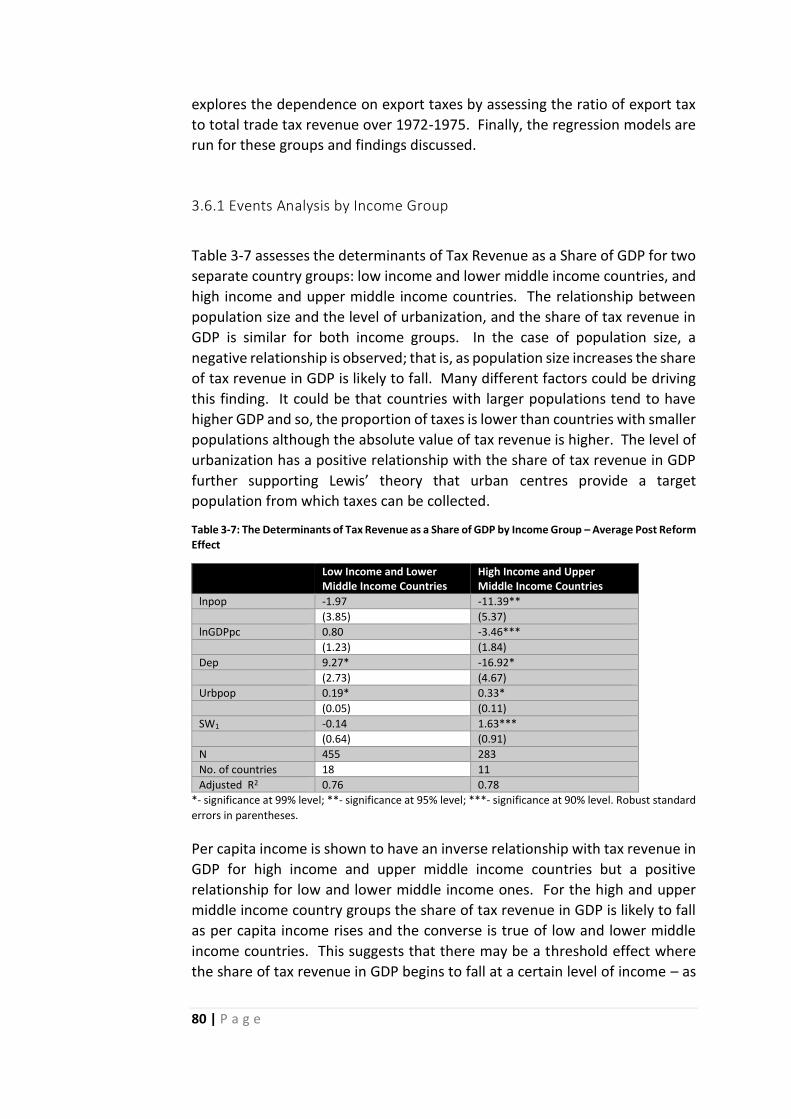
80 | P a g e

explores the dependence on export taxes by assessing the ratio of export tax

to total trade tax revenue over 1972-1975. Finally, the regression models are

run for these groups and findings discussed.

3.6.1 Events Analysis by Income Group

Table 3-7 assesses the determinants of Tax Revenue as a Share of GDP for two

separate country groups: low income and lower middle income countries, and

high income and upper middle income countries. The relationship between

population size and the level of urbanization, and the share of tax revenue in

GDP is similar for both income groups. In the case of population size, a

negative relationship is observed; that is, as population size increases the share

of tax revenue in GDP is likely to fall. Many different factors could be driving

this finding. It could be that countries with larger populations tend to have

higher GDP and so, the proportion of taxes is lower than countries with smaller

populations although the absolute value of tax revenue is higher. The level of

urbanization has a positive relationship with the share of tax revenue in GDP

further supporting Lewis’ theory that urban centres provide a target

population from which taxes can be collected.

Table 3-7: The Determinants of Tax Revenue as a Share of GDP by Income Group – Average Post Reform

Effect

Low Income and Lower Middle Income Countries

High Income and Upper Middle Income Countries

lnpop -1.97 -11.39**

(3.85) (5.37)

lnGDPpc 0.80 -3.46***

(1.23) (1.84)

Dep 9.27* -16.92*

(2.73) (4.67)

Urbpop 0.19* 0.33*

(0.05) (0.11)

SW1 -0.14 1.63***

(0.64) (0.91)

N 455 283

No. of countries 18 11

Adjusted R2 0.76 0.78

*- significance at 99% level; **- significance at 95% level; ***- significance at 90% level. Robust standard

errors in parentheses.

Per capita income is shown to have an inverse relationship with tax revenue in

GDP for high income and upper middle income countries but a positive

relationship for low and lower middle income ones. For the high and upper

middle income country groups the share of tax revenue in GDP is likely to fall

as per capita income rises and the converse is true of low and lower middle

income countries. This suggests that there may be a threshold effect where

the share of tax revenue in GDP begins to fall at a certain level of income – as

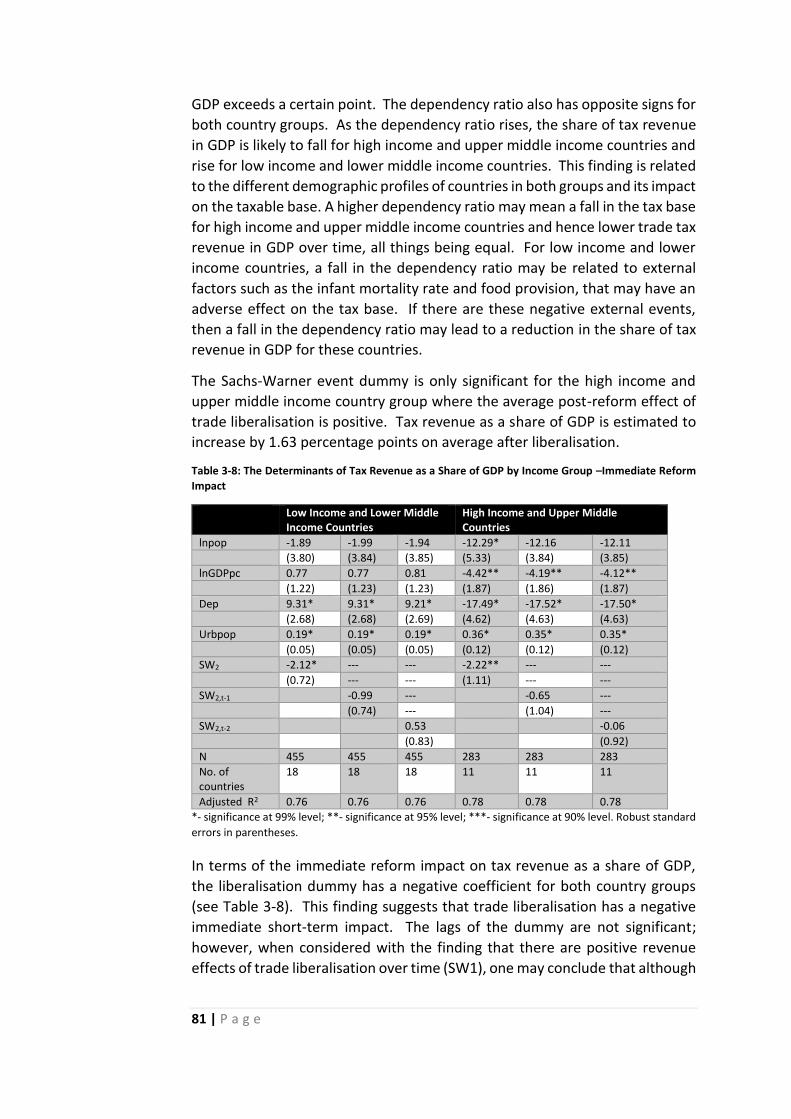
81 | P a g e

GDP exceeds a certain point. The dependency ratio also has opposite signs for

both country groups. As the dependency ratio rises, the share of tax revenue

in GDP is likely to fall for high income and upper middle income countries and

rise for low income and lower middle income countries. This finding is related

to the different demographic profiles of countries in both groups and its impact

on the taxable base. A higher dependency ratio may mean a fall in the tax base

for high income and upper middle income countries and hence lower trade tax

revenue in GDP over time, all things being equal. For low income and lower

income countries, a fall in the dependency ratio may be related to external

factors such as the infant mortality rate and food provision, that may have an

adverse effect on the tax base. If there are these negative external events,

then a fall in the dependency ratio may lead to a reduction in the share of tax

revenue in GDP for these countries.

The Sachs-Warner event dummy is only significant for the high income and

upper middle income country group where the average post-reform effect of

trade liberalisation is positive. Tax revenue as a share of GDP is estimated to

increase by 1.63 percentage points on average after liberalisation.

Table 3-8: The Determinants of Tax Revenue as a Share of GDP by Income Group –Immediate Reform

Impact

Low Income and Lower Middle Income Countries

High Income and Upper Middle Countries

lnpop -1.89 -1.99 -1.94 -12.29* -12.16 -12.11

(3.80) (3.84) (3.85) (5.33) (3.84) (3.85)

lnGDPpc 0.77 0.77 0.81 -4.42** -4.19** -4.12**

(1.22) (1.23) (1.23) (1.87) (1.86) (1.87)

Dep 9.31* 9.31* 9.21* -17.49* -17.52* -17.50*

(2.68) (2.68) (2.69) (4.62) (4.63) (4.63)

Urbpop 0.19* 0.19* 0.19* 0.36* 0.35* 0.35*

(0.05) (0.05) (0.05) (0.12) (0.12) (0.12)

SW2 -2.12* --- --- -2.22** --- ---

(0.72) --- --- (1.11) --- ---

SW2,t-1 -0.99 --- -0.65 ---

(0.74) --- (1.04) ---

SW2,t-2 0.53 -0.06

(0.83) (0.92)

N 455 455 455 283 283 283

No. of countries

18 18 18 11 11 11

Adjusted R2 0.76 0.76 0.76 0.78 0.78 0.78

*- significance at 99% level; **- significance at 95% level; ***- significance at 90% level. Robust standard

errors in parentheses.

In terms of the immediate reform impact on tax revenue as a share of GDP,

the liberalisation dummy has a negative coefficient for both country groups

(see Table 3-8). This finding suggests that trade liberalisation has a negative

immediate short-term impact. The lags of the dummy are not significant;

however, when considered with the finding that there are positive revenue

effects of trade liberalisation over time (SW1), one may conclude that although

82 | P a g e

trade tax revenue may decline initially, other sources, such as domestic taxes,

will eventually be substituted to replace lost revenue.

Similar to the average effects model in Table 3-7, the model also predicts that

as the level of urbanization increases so will the share of tax revenue in GDP.

Population size is shown to have a negative relationship with the share of tax

revenue in GDP. The dependency ratio has a positive relationship with the

dependent variable for low income and lower middle income countries and a

negative relationship for high and upper middle income countries. Finally, per

capita income is shown to vary inversely with tax revenue as a share of GDP

for high and upper middle income countries and positively for low income and

lower middle income countries.

Table 3-9: The Determinants of Trade Tax Revenue as a Share of GDP by Income Group – Average Post

Reform Effect

Low and Lower Middle Income Countries

High and Upper Middle Income Countries

lnpop 5.49** -6.46*

(2.15) (1.46)

lnGDPpc -0.14* -2.16*

(0.58) (0.64)

DTaxgdp -0.24* -0.14**

(0.06) (0.06)

ER 0.00** 0.00

(0.00) (0.00)

Dep 3.26*** -7.18*

(1.87) (1.92)

Urbpop 0.06** -0.02

(0.03) (0.03)

SW1 -0.15 0.06

(0.33) (0.39)

N 434 246

No. of countries 18 11

Adjusted R2 0.67 0.85

*- significance at 99% level; **- significance at 95% level; ***- significance at 90% level. Robust standard

errors in parentheses.

For the model estimating the determinants of trade tax revenue as a share of

GDP over time (see Table 3-9), per capita income and the share of domestic

taxes in GDP are shown to have a negative relationship with the dependent

variable for both income groups. This is consistent with the a priori

expectation that at higher income levels, countries show a preference for

domestic taxes over border taxes due to ease of administration. In addition, a

fall in the exchange rate is likely to reduce the share of trade tax revenue in

GDP as ceteris paribus, a fall in the exchange rate makes imports more

expensive and exports less so. The final effect depends on which effect

dominates and elasticities of demand and supply. It should be noted, however,

that the coefficient on the exchange rate is very small and so, this effect is

minimal.

83 | P a g e

Population size is shown to have a positive relationship with the share of trade

tax revenue in GDP for low and lower middle income countries. In contrast,

trade tax revenue is likely fall as population size increases for high and upper

middle income countries. Although population size is a used as a rough

indicator of the taxable base, it is clear that there is an interplay with a

country’s level development which may determine the extent to which trade

tax revenue can be collected. The dependency ratio also has opposite signs

for both income groups. For low and lower middle income countries, the

share of trade tax revenue in GDP is expected to fall as the dependency ratio

falls; the converse is true for high and upper middle income countries.

The level of urbanisation has a positive and significant relationship with trade

tax revenue as a share of GDP for low and lower middle income countries while

a positive, but insignificant relationship, is seen for high and upper middle

income countries. The liberalisation event dummies are not significant for

both income groups, which suggests that there is no significant effect on trade

tax revenue as a share of GDP, in the years after trade reform.

Table 3-10: The Determinants of Trade Tax Revenue as a Share of GDP by Income Group - Immediate

Reform Impact

Low Income and Lower Middle Income Countries

High Income and Upper Middle Countries

lnpop 5.46** 5.49** 5.54** -6.47* -6.47* -6.47*

(2.15) (2.15) (2.15) (1.45) (1.45) (1.45)

lnGDPpc -0.15 -0.13 -0.11 -2.15* -2.16* -2.16*

(0.58) (0.58) (0.58) (0.59) (0.59) (0.58) DTaxgdp -0.24* -0.24* -0.24* -0.14** -0.14** -0.14** (0.06) (0.06) (0.06) (0.06) (0.06) (0.06) ER 0.00* 0.00* 0.00* 0.00 0.00 0.00 (0.00) (0.00) (0.00) (0.00) (0.00) (0.00)

Dep 3.24*** 3.21*** 3.17*** -7.20* -7.18* -7.19*

(1.87) (1.87) (1.87) (1.91) (1.91) (1.91)

Urbpop 0.06** 0.06** 0.06** -0.02 -0.02 -0.02

(0.03) (0.03) (0.03) (0.04) (0.04) (0.04)

SW2 -0.56 --- --- 0.28 --- ---

(0.36) --- --- (0.35) --- ---

SW2,t-1 -0.07 --- 0.23 ---

(0.44) --- (0.38) ---

SW2,t-2 0.55 0.24

(0.44) (0.45)

N 434 434 434 246 246 246

No. of countries

18 18 18 11 11 11

Adjusted R2 0.67 0.67 0.67 0.85 0.85 0.85

*- significance at 99% level; **- significance at 95% level; ***- significance at 90% level. Robust standard

errors in parentheses.

With respect to the immediate impact of trade liberalisation on trade tax

revenue as a share of GDP (see Table 3-10), the event dummies are also not

84 | P a g e

significant. In the model, no evidence was found of a significant impact in the

year of liberalisation and in the one to two-year period following liberalisation.

However, recall that the model found a negative and significant relationship

between share of total tax revenue in GDP and trade liberalisation on average

post-reform for the high income and upper middle income country group

(mainly upper middle income countries). As trade liberalisation is part of an

integrated process of broader economic reform, high and upper middle

income countries may find it easier to incorporate changes to their tax system

(such as increased use of domestic taxes) given that they have more advanced

tax systems than their less developed counterparts. In addition, over the long

term, the effect of trade liberalisation on total tax revenue was found to be

positive in the years after liberalisation. This may be due to an increased ability

of high and upper middle income countries to take advantage of the economic

opportunities brought about by trade liberalisation.

Similar to the model that assesses the average effect of trade liberalisation

over time, domestic taxes as a share of GDP and per capita income are shown

to vary inversely with the share of trade tax revenue in GDP for both country

groups. As the share of domestic taxes in GDP rises, the model predicts that

the share of trade tax revenue will fall. This suggests that countries do replace

trade taxes with domestic taxes over time due to ease of collection and

distributional concerns, among other factors. In addition, as per capita income

increases, the share of trade tax revenue is GDP is likely to fall. As an indicator

of the level of development, a rise in per capita income means that countries

are becoming more developed and therefore, better able to diversify the tax

base, in particular, extend the coverage of domestic taxes. Also, another factor

that may explain this relationship is that industries that may have benefitted

from high tariffs on imports in the early stages of development may see those

protective measures removed as they mature.

In addition, the exchange rate has a positive relationship with the share of

trade tax revenue in GDP. An increase in the exchange rate (appreciation)

makes imports less expensive and exports costlier. The effect in the model is

estimated to be extremely small, however, and to not be significant for high

and upper middle income countries. Population size is shown to have a

negative relationship with the share of trade tax revenue in GDP for high and

upper middle income but a positive one for low and lower middle income

countries. It may be the case that as population size increases for upper and

middle income countries, there is an increase in the taxable base for

alternative taxes, such as consumption taxes, which further reduce the trade

tax revenue share in GDP. The converse may occur in low income and lower

middle countries that still have trade tax revenue as a major source of income

and so, an increase in the population may mean increased consumption of

imported products and therefore, an increase in trade tax revenue at a lower

rate than the rate of GDP growth.

85 | P a g e

The level of urbanisation is found to vary positively with the share of trade tax

revenue is GDP for low and lower middle income countries, suggesting that as

these countries become more urbanised the share of trade tax revenue was

likely to rise by about 0.06%. In this case, the countries at this level of

development are not likely to have a sufficiently developed tax system to

replace trade taxes with domestic taxes; however, with urbanisation, they may

be better able to centrally locate customs services, etc. and thus, improve the

collection of trade tax revenue. On the other hand, for high and upper middle

income countries that are at a different level of development, a significant

relationship is not found between the level of urbanisation and trade tax

revenue as a share of GDP. Arguably, most of these countries would have

already been urban throughout the sample period and one would therefore

not expect any significant change in trade tax revenue as a result of changes in

the level of urbanisation.

In addition, the model predicts that a fall in the dependency ratio is likely to

lead to a reduction in the share of trade tax revenue in GDP for low and lower

middle income countries. On the other hand, as the dependency ratio rises, it

is likely to lead to a fall in trade tax revenue as a share of GDP in high income

and upper middle income countries. The variation in findings may be due to

the different demographic characteristics of both income groups and its

impact on the taxable base. For high income and upper middle income

countries, a higher dependency ratio may mean a fall in the tax base and hence

lower trade tax revenue in GDP over time, all things being equal. Health, social

and environmental facts may influence a reduction in the dependency ratio in

low income and lower income countries. They may also have an adverse effect

on the tax base and by extension, the share of tax revenue in GDP for these

countries.

The results of the events analysis suggest that there are significant differences

between high income and upper middle income, and low income and lower

middle income countries with respect to the interaction of key variables and

the total tax and trade tax revenue as a share of GDP. Importantly, the results

suggest that the impact of trade liberalisation is at the aggregate tax revenue

level. While the overall average effect is estimated to be positive and

significant for only high income and upper middle income countries, the short-

term impact (within a year of the liberalisation event) is negative for both

country income groups. There is also no evidence that there are significant

lagged effects of trade liberalisation within one and two years of the reform

date.

In addition to the variation in the sample by country size, there are also likely

to be differences in the implementation of the reforms themselves which are

likely to be influenced by the existing trade tax structure. The majority of

analyses tend to concentrate on how the structure of import taxes affects the

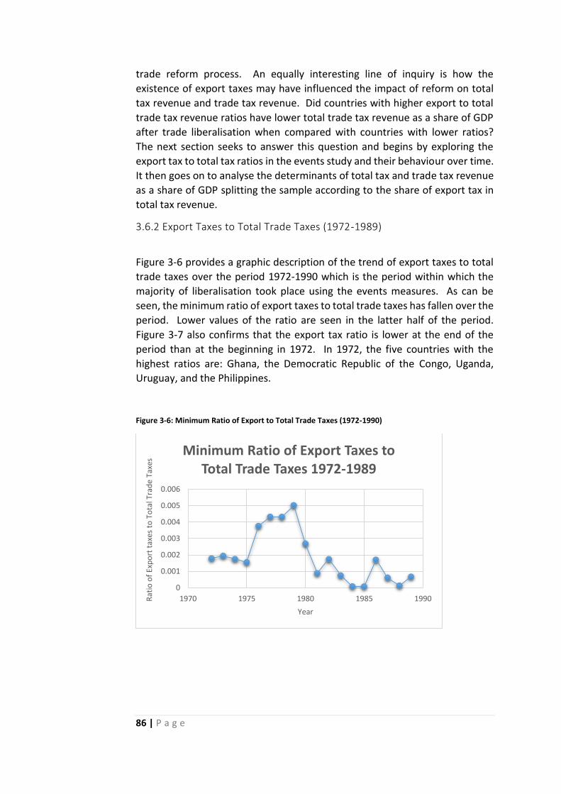
86 | P a g e

trade reform process. An equally interesting line of inquiry is how the

existence of export taxes may have influenced the impact of reform on total

tax revenue and trade tax revenue. Did countries with higher export to total

trade tax revenue ratios have lower total trade tax revenue as a share of GDP

after trade liberalisation when compared with countries with lower ratios?

The next section seeks to answer this question and begins by exploring the

export tax to total tax ratios in the events study and their behaviour over time.

It then goes on to analyse the determinants of total tax and trade tax revenue

as a share of GDP splitting the sample according to the share of export tax in

total tax revenue.

3.6.2 Export Taxes to Total Trade Taxes (1972-1989)

Figure 3-6 provides a graphic description of the trend of export taxes to total

trade taxes over the period 1972-1990 which is the period within which the

majority of liberalisation took place using the events measures. As can be

seen, the minimum ratio of export taxes to total trade taxes has fallen over the

period. Lower values of the ratio are seen in the latter half of the period.

Figure 3-7 also confirms that the export tax ratio is lower at the end of the

period than at the beginning in 1972. In 1972, the five countries with the

highest ratios are: Ghana, the Democratic Republic of the Congo, Uganda,

Uruguay, and the Philippines.

Figure 3-6: Minimum Ratio of Export to Total Trade Taxes (1972-1990)

0

0.001

0.002

0.003

0.004

0.005

0.006

1970 1975 1980 1985 1990Rat

io o

f Ex

po

rt t

axes

to

To

tal T

rad

e Ta

xes

Year

Minimum Ratio of Export Taxes to Total Trade Taxes 1972-1989

87 | P a g e

Figure 3-7: Ratio of Export Taxes to Total Trade Taxes (1972 and 1989)

Table 3-11 ranks countries by the highest value of the export tax to total tax ratio over the period 1972-1975. The highest value is 0.84, which belongs to Ghana. A little less than fifty percent of countries (12) in the sample have an export tax to total tax ratio below 0.081. The countries with export taxes mainly comprise developing countries, ranging from low income to upper middle income countries. The rankings show broad heterogeneity across income groups.

Table 3-11: Ratio of Export Taxes to Total Trade Taxes in Descending Order of the Highest Value over

1972-1975 – Top 15 in Sample

Country Highest value over 1972-1975 Average over 1972-1975

Guyana 0.84 0.44

Uruguay 0.78 0.49

Ghana 0.67 0.65

Malaysia 0.51 0.40

Mauritius 0.41 0.29

Pakistan 0.39 0.32

Nicaragua 0.38 0.17

Ecuador 0.36 0.29

Sri Lanka 0.35 0.30

Thailand 0.34 0.18

Philippines 0.29 0.25

The Gambia 0.22 0.17

Mexico 0.21 0.17

Morocco 0.19 0.13

Tunisia 0.17 0.07

Of the twenty-nine countries in the events study, twenty-two imposed export taxes over the period. It would be instructive to note if there is a significant difference in the impact of trade liberalisation (as denoted by the Sachs-

0.2

.4.6

.8

Expo

rt T

ax to T

ota

l T

rad

e T

ax R

atio

Countries

1972 1989

Ratio of Export Taxes to Total Trade Taxes (1972 and 1989)

88 | P a g e

Warner liberalisation event) on total tax and trade tax revenue when export taxes are above and below the median point of 8% of Total Trade Tax revenue. Although the median ratio appears relatively low, it sets a base of comparison for countries with respect to the extent to which they would need to replace export tax revenue in the reform process. It also allows one to assess if there is any difference in the impact of liberalisation on total tax revenue and trade tax revenue between the two groups. The regression models for the determinants of trade tax and total tax revenue as a share of GDP continue to be used for this section. The models are run for countries with export tax to total trade tax revenue ratios above and below the median level.

3.6.3 Events Analysis by Share of Export Tax to Total Trade Tax

For the determinants of tax revenue as a share of GDP, there are clear

differences in the results for countries above and below the median ratio. For

countries with export to total trade tax ratios below 0.08 in the initial five years

of the study (1972-1975), an inverse and significant relationship is found

between population size and the level of urbanization, and the share of total

tax revenue in GDP (see Table 3-12). A significant positive relationship is also

found between per capita income and total tax revenue as a share of GDP.

Table 3-12: The Determinants of Tax Revenue as a Share of GDP by Export Tax Revenue to Total Trade

Tax Revenue Ratio – Average Post Reform Effect

Export Tax to Total Trade Tax Revenue Ratio<0.08

Export Tax to Total Trade Tax Revenue Ratio>0.08

lnpop -5.88* 8.58*

(1.98) (3.22)

lnGDPpc 6.33* -0.76

(1.02) (1.41)

Dep 3.02 -1.88

(3.01) (2.65)

Urbpop -0.14* 0.15*

(0.06) (0.06)

SW1 2.37* -2.49*

(0.69) (0.80)

N 289 349

No. of countries 12 13

Adjusted R2 0.91 0.76

*- significance at 99% level; **- significance at 95% level; ***- significance at 90% level. Robust standard

errors in parentheses.

On the other hand, a positive and significant relationship is found between

population size and the level of urbanization, and the share of total tax revenue

in GDP for countries with export to total trade tax ratios above the median

level. Per capita income is not found to be a significant variable for these

countries. For both groups, the dependency ratio is not a significant variable.

These findings are likely driven by the diverse characteristics of countries in

89 | P a g e

both groups. Both groups included countries from all income levels; for

example, the group above the median export to total tax ratio, included South

Africa, Mexico and The Gambia. It would appear that more high and upper

middle income groups appear to be in the group above the median total tax

ratio and the result reported with respect to per capita income is consistent

with the sign to obtained for the model with high income countries.

With respect to the liberalisation event, the results show that there was a

positive effect on total tax revenue for countries below the median ratio.

However, countries with export tax to total trade tax ratios above the median

level, were likely to see negative effects of the share of total tax revenue in

GDP, falling by 2.49 percentage points on average in the period after trade

liberalisation, as denoted by the Sachs-Warner event dummy.

Table 3-13: The Determinants of Tax Revenue as a Share of GDP by Export Tax Revenue to Total Trade

Tax Revenue –Immediate Reform Impact

Export Tax to Total Tax Revenue Ratio<0.08

Export Tax to Total Tax Revenue Ratio>0.08

lnpop -5.74* -5.94* -6.03* 8.00** 8.00** 8.04**

(1.99) (2.01) (2.01) (3.24) (3.26) (3.26)

lnGDPpc 6.58* 6.62* 6.69* -0.99 -0.96 -0.95

(1.05) (1.05) (1.06) (1.43) (1.43) (1.43)

Dep 2.47 2.53 2.52 -2.02 -2.09 -2.11

(3.10) (3.12) (3.12) (2.66) (2.67) (2.67)

Urbpop -0.17* -0.16* -0.16* 0.14** 0.14** 0.14**

(0.06) (0.06) (0.06) (0.06) (0.06) (0.06)

SW2 -1.91 --- --- -2.28* --- ---

(0.73) --- --- (0.75) --- ---

SW2,t-1 -0.01 --- -1.13 ---

(0.72) --- (0.76) ---

SW2,t-2 1.15 -0.38

(0.81) (0.67)

N 289 289 289 349 349 349

No. of countries

12 12 12 13 13 13

Adjusted R2 0.91 0.91 0.91 0.76 0.76 0.76

*- significance at 99% level; **- significance at 95% level; ***- significance at 90% level. Robust standard

errors in parentheses.

Regarding the immediate reform impact on tax revenue as a share of GDP (see

Table 3-13), the liberalisation dummy is not significant for countries below the

median export tax to trade tax ratio. However, there is a significant negative

effect on the share of total tax revenue in GDP within the first year of

liberalisation for countries with trade tax revenue above the median ratio.

There is no significant lagged effect on the share of total tax revenue in GDP

within one and two years of liberalisation for countries in both groups.

As found in the average effects model in Table 3-12, significant negative

relationships are found between the population size and the level of

urbanization and the share of total revenue in GDP for countries below the

median export to total trade tax ratio. For countries above the median ratio,

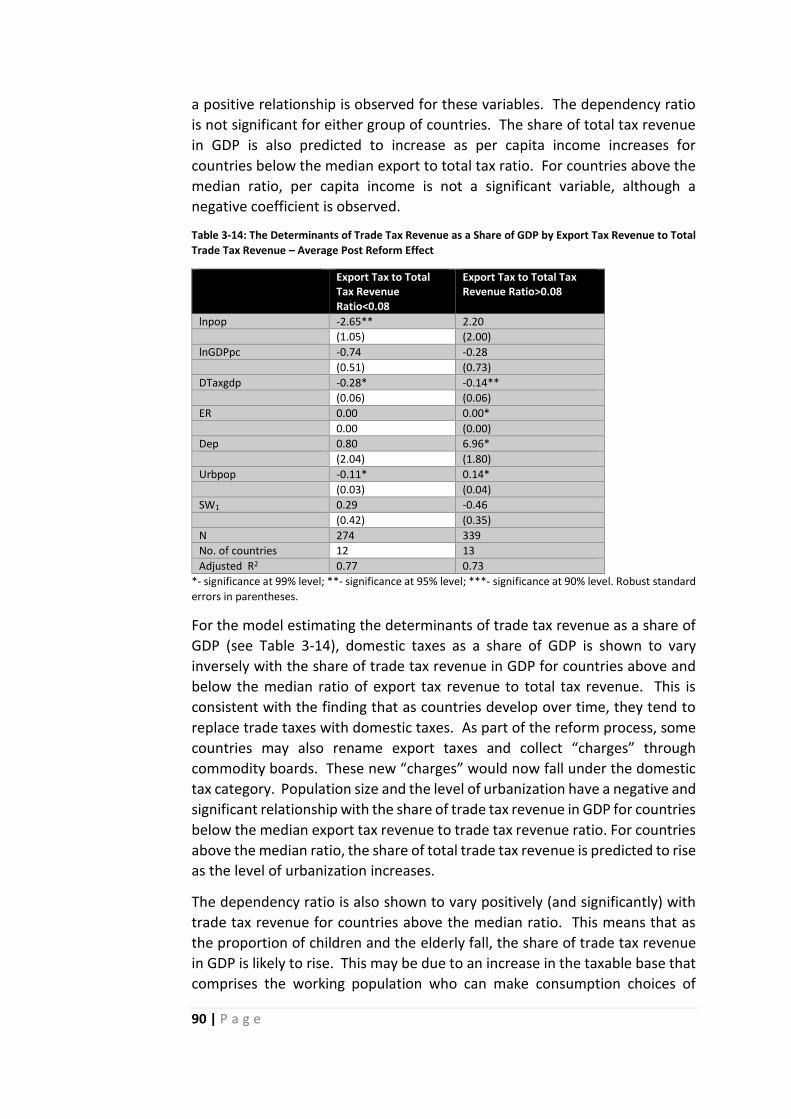
90 | P a g e

a positive relationship is observed for these variables. The dependency ratio

is not significant for either group of countries. The share of total tax revenue

in GDP is also predicted to increase as per capita income increases for

countries below the median export to total tax ratio. For countries above the

median ratio, per capita income is not a significant variable, although a

negative coefficient is observed.

Table 3-14: The Determinants of Trade Tax Revenue as a Share of GDP by Export Tax Revenue to Total

Trade Tax Revenue – Average Post Reform Effect

Export Tax to Total Tax Revenue Ratio<0.08

Export Tax to Total Tax Revenue Ratio>0.08

lnpop -2.65** 2.20

(1.05) (2.00)

lnGDPpc -0.74 -0.28

(0.51) (0.73)

DTaxgdp -0.28* -0.14**

(0.06) (0.06)

ER 0.00 0.00*

0.00 (0.00)

Dep 0.80 6.96*

(2.04) (1.80)

Urbpop -0.11* 0.14*

(0.03) (0.04)

SW1 0.29 -0.46

(0.42) (0.35)

N 274 339

No. of countries 12 13

Adjusted R2 0.77 0.73

*- significance at 99% level; **- significance at 95% level; ***- significance at 90% level. Robust standard

errors in parentheses.

For the model estimating the determinants of trade tax revenue as a share of

GDP (see Table 3-14), domestic taxes as a share of GDP is shown to vary

inversely with the share of trade tax revenue in GDP for countries above and

below the median ratio of export tax revenue to total tax revenue. This is

consistent with the finding that as countries develop over time, they tend to

replace trade taxes with domestic taxes. As part of the reform process, some

countries may also rename export taxes and collect “charges” through

commodity boards. These new “charges” would now fall under the domestic

tax category. Population size and the level of urbanization have a negative and

significant relationship with the share of trade tax revenue in GDP for countries

below the median export tax revenue to trade tax revenue ratio. For countries

above the median ratio, the share of total trade tax revenue is predicted to rise

as the level of urbanization increases.

The dependency ratio is also shown to vary positively (and significantly) with

trade tax revenue for countries above the median ratio. This means that as

the proportion of children and the elderly fall, the share of trade tax revenue

in GDP is likely to rise. This may be due to an increase in the taxable base that

comprises the working population who can make consumption choices of

91 | P a g e

traded goods. However, the dependency ratio is not significant for countries

above the median export tax to trade tax revenue ratio.

Per capita income is not a significant variable for either country group. It

should also be noted that the exchange rate is shown to have a positive

relationship with trade tax revenue in GDP, which is significant for countries

above the median export tax to total trade tax revenue. A reduction in the

exchange rate is likely to reduce the share of trade tax revenue in GDP as

ceteris paribus, a fall in the exchange rate makes imports more expensive and

exports less so. The final effect depends on which effect dominates and

elasticities of demand and supply. However, the effect on trade tax revenue

as a share of GDP is minimal in the model. With respect to the trade

liberalisation event, there is no significant effect on trade tax revenue as a

share of GDP on average in the years after liberalisation for either country

group.

Table 3-15: The Determinants of Trade Tax Revenue as a Share of GDP by Export Tax Revenue to Total

Trade Tax Revenue - Immediate Reform Impact

Export to Total Tax Ratio<0.08 Export to Total Tax Ratio>0.08

lnpop -2.71* -2.69* -2.64** 2.06 2.08 2.10

(1.03) (1.04) (1.04) (1.99) (1.99) (1.98)

lnGDPpc -0.72 -0.70 -0.66 -0.31 -0.30 -0.30

(0.53) (0.53) (0.53) (0.73) (0.73) (0.73) DTaxgdp -0.29* -0.29* -0.28* -0.14** -0.13** -0.13** (0.06) (0.06) (0.06) (0.06) (0.06) (0.06) ER 0.00 0.00 0.00 0.00* 0.00* 0.00* 0.00 0.00 0.00 (0.00) (0.00) (0.00)

Dep 0.77 0.80 0.76 6.91* 6.90* 6.91*

(2.04) (2.05) (2.06) (1.81) (1.80) (1.80)

Urbpop -0.11* -0.11* -0.11* 0.14* 0.14* 0.14*

(0.03) (0.03) (0.03) (0.04) (0.04) (0.04)

SW2 -0.52 --- --- -0.22 --- ---

(0.46) --- --- (0.28) --- ---

SW2,t-1 0.04 --- 0.12 ---

(0.52) --- (0.32) ---

SW2,t-2 0.83*** 0.42

(0.43) (0.41)

N 274 274 274 339 339 339

No. of countries

12 12 12 13 13 13

Adjusted R2 0.77 0.77 0.77 0.73 0.73 0.73

*- significance at 99% level; **- significance at 95% level; ***- significance at 90% level. Robust standard

errors in parentheses.

With respect to the immediate impact of trade liberalisation on trade tax

revenue as a share of GDP (see Table 3-15), the results of the model show that

trade liberalisation had no immediate impact on trade tax revenue as a share

of GDP within the year of the liberalisation for countries below the median

export tax to total tax ratio. There also is no impact on trade tax revenue seen

within a year of liberalisation; however, there is some impact within two years

92 | P a g e

of liberalisation for these countries. Trade tax revenue is predicted to fall by -

0.83 percentage points two years after trade liberalisation. For countries

above the median ratio, no immediate impact is seen in the year of

liberalisation, nor within one and two years of the liberalisation event.

However, it should be recalled that effects at the aggregate level on total tax

revenue were seen. This supports the theory that trade liberalisation often

forms part of a comprehensive macroeconomic reform programme that may

include reforms to domestic taxes and incentive structures. The overall impact

of this process may therefore be more likely to be observed at the aggregate

level rather than on trade tax revenue itself.

Domestic taxes as a share of GDP is shown to have a negative relationship with

the share of trade tax revenue in GDP for both country groups. As the share

of domestic taxes in GDP increases, the model predicts that the share of trade

tax revenue will decrease. This suggests that there may be some replacement

of trade taxes with domestic taxes over time due to administrative efficiencies,

among other factors. In addition, the exchange rate has a positive relationship

with the share of trade tax revenue in GDP, which is significant for countries

above the median ratio of export tax to total trade tax revenue. An

appreciation of the exchange rate makes imports less expensive and exports

more so; the final effect being determined by demand and supply elasticities.

Again, the effect in the model is estimated to be extremely small.

Population size and the level of urbanization are shown to vary inversely and

significantly with the share of trade tax revenue in GDP for countries below the

median export tax revenue to trade tax revenue ratio. On the other hand, a

significant relationship is not seen for countries above the median ratio with

respect to population size. The share of trade tax revenue in GDP is likely to

increase with an increase in the level of urbanization for countries below the

median ratio.

The dependency ratio is also shown to vary positively with the share of trade

tax revenue in GDP for countries both country groups, with a significant

relationship for countries above the median ratio. This may be due to an

increase in the taxable base that comprises the working population who can

make consumption choices of traded goods. Per capita income is not a

significant variable for either country group.

The results of the events analysis by export tax ratio suggest that there are

significant differences among countries when split into groups by the ratio of

export tax to total tax revenue. The findings reaffirm that there are tangible

differences between countries that require a tailored approach to

liberalisation. In addition, with respect to the question of whether there was

any difference in the impact of trade liberalisation on countries based on their

initial export tax to total tax ratio, countries above the median ratio were

93 | P a g e

predicted to see an average negative effect on the share of total tax revenue

in GDP over time while those below the median ratio were likely to see a

positive effect on total tax revenue as a share of GDP. The short-term effect

of trade liberalisation on total tax and trade tax revenue itself is not significant,

with the exception of a two-year lag for countries that was found to be

significant for countries with export tax to trade tax revenue ratios above the

median level. The effect of trade liberalisation, as denoted by the Sachs-

Warner event are therefore manifested over time at an aggregate level and

therefore depend on the interplay of the entire economic reform programme,

of which trade liberalisation is often just one component.

3.7 Conclusions

This chapter explored an alternative framework to examine the impact of trade

reform on total tax revenue and trade tax revenue as a share of GDP. Trade

liberalisation is often driven by external events and shocks such as a severe

decline in the balance of payments and lack of access to global financial

markets. Countries (mainly developing) facing these constraints turned to

multilateral lending institutions, such as the IMF and World Bank, for

assistance. In most cases, trade reform was included as part of a

comprehensive economic reform programme with strict conditionalities for

continued financing under these loan agreements. Since these “events” are

the driving force behind reforms, it makes sense to utilise an events framework

to analyse the impact of trade reform on total tax and trade tax revenue. Three

events measures were used based on work by Sachs-Warner (1995), Dean et

al. (1994) and Greenaway et al. (2005). In the first scenario, the setup of the

event dummies sought to capture the average effect of trade reform on total

tax revenue as a share of GDP. The second variation of the event dummies

captured the immediate impact of liberalisation on the dependent fiscal

revenue variables. The models were also run with lags of the event dummies

to see if there are impacts within one and two years of liberalisation.

In general, trade liberalisation as captured by events was not a significant

determinant of changes in total or trade tax revenues; in the vast majority of

cases the dummy variable was insignificant. There is weak evidence that trade

liberalisation, as denoted by the Sachs-Warner dummy, was associated with

an increase in the share of total tax revenue in GDP (by 0.87 percentage points

on average in the years after liberalisation). The average post-reform effect

as measured by the Dean et al. (1994) and World Bank dummies, although

having a negative sign, is not significant. The immediate impact of the

liberalisation is a reduction in total tax revenue as a share of GDP by 1.72

percentage points in the year of liberalisation event, as measured by the Sachs-

Warner dummy. The other event dummies are not significant; although, there

94 | P a g e

is a small negative coefficient for the Dean dummy and a small positive

coefficient on the World Bank dummy. The lagged values of the event

dummies are not significant which suggests that there are no significant effects

on the share of total tax revenue within one to two years of the liberalisation

event.

The results also suggest that there may be a negative impact on total tax

revenue as a share of GDP within the year of liberalisation but the long-run

average effect is likely to be positive. This is not surprising as trade

liberalisation is often a part of a comprehensive reform programme that

includes other components such as exchange rate adjustment and broader tax

reform. If, for example, there are changes to domestic taxes and exchange

rate adjustments, then the final impact will be shown at the aggregate tax

revenue level after the reforms have worked through the economy, taking into

account factors such as supply and demand of imports and domestic

substitutes and the administrative capacity of the state to collect taxes. Since

the other event measures are not significant in the models, it is clear that the

findings are sensitive to the measure of trade liberalisation used and in

particular, the dating of the liberalisation event and the sample chosen.

With respect to the share of trade tax revenue in GDP, none of the

liberalisation event dummies is significant for any of the models. This suggests

that trade liberalisation did not have any significant effect on total trade tax

revenue as a share of GDP on average in the years following liberalisation. The

effect on trade tax revenue as a share of GDP depends on the nature of reforms

and timing and sequencing, among other factors. A gradual reduction in tariffs

and replacement with indirect taxes are less likely to lead to significant

changes in the share of trade tax revenue in GDP. Another consideration is the

pace of GDP growth. Once a country’s rate of GDP growth exceeds growth in

trade tax revenue as a share of GDP, one can expect that the trade tax revenue

as a share of GDO will fall.

Trade liberalisation does not have an immediate impact on the share of total

trade taxes as a share of GDP as the event dummies are not significant. The

one and two-year lags of the dummies are also not significant, which suggests

that there is no discernible impact of the share of trade tax revenue in GDP as

a result of trade liberalisation using the event indicators under study.

When the models are assessed based on country groups – high and upper

middle income countries, and low and lower middle income countries, there

are significant differences in the impact of trade liberalisation on total tax and

trade tax revenue. Trade liberalisation is shown to have an average positive

effect on total tax revenue as a share of for the high income and upper middle

income country group GDP, by the Sachs-Warner measure. However, the

immediate reform impact on tax revenue as a share of GDP is negative and

95 | P a g e

significant for both country groups. The lags of the dummy are not significant,

which means that the effect is not carried forward into subsequent years.

These findings support the conclusion that while there may be a negative

effect initially of trade reform on total tax revenue as a share of GDP on both

country groups, the average effect is likely to be positive for high and upper

middle income countries in the long run. High and upper middle income

countries have more developed economies and administrative systems that

may make it easier to replace any income lost from liberalisation with revenue

from other sources. In addition, the composition and execution of a wider

reform programme is likely to influence the final effect on total tax revenue as

a share of GDP. The study found no evidence that trade liberalisation impacts

trade tax revenue as a share of GDP on average in the years after reform or in

the short-term in both country groups.

The results of the analysis by the share of export tax revenue in total tax

revenue show that the impact of trade liberalisation on total tax and trade tax

revenue as a share of GDP is different for those countries above and below the

median threshold. Countries with ratios above the median level were likely to

see negative effects of the share of total tax revenue in GDP, as denoted by

the Sachs-Warner event dummy. No significant short-term impact is found for

countries below the median export tax to trade tax ratio. However, there is a

significant negative effect on the share of total tax revenue in GDP within the

first year of liberalisation for countries with trade tax revenue above the

median ratio. There is no significant lagged effect on the share of total tax

revenue in GDP within one and two years of liberalisation for countries in both

groups.

There is no significant effect on trade tax revenue as a share of GDP on average

in the years after liberalisation for either country group. The results also show

that trade liberalisation has no immediate impact on trade tax revenue as a

share of GDP within the year of the liberalisation for countries below the

median export tax to total tax ratio. There also is no impact on trade tax

revenue seen within a year of liberalisation; however, there is some impact

within two years of liberalisation for these countries.

The overall impact of trade liberalisation on fiscal revenue is therefore more

likely to be observed at the aggregate level rather than on trade tax revenue

itself. Trade liberalisation usually forms part of a reform programme that

covers broader economic and systemic reforms that may have a net positive

or negative effect on the economy and indirectly on total tax revenue. The

Sachs-Warner index captures some of these reforms and the average effect of

trade liberalisation on total tax revenue as a share of GDP over time is shown

to be positive and significant.

96 | P a g e

It is clear that the findings of the models are sensitive to the measure of trade

liberalisation used and in particular, the dating of the liberalisation event and

the associated sample. There is much room for further analysis in this area to

find better ways of measuring the net impact of liberalisation on government

revenue. In addition, other methods for events analysis could be explored

that are applicable to a larger number of countries. As the revenue effects

observed are at the aggregate level, it would be useful to analyse the net effect

of trade liberalisation by using a general equilibrium model that can take

account of the complex relationships in the domestic economy, the

adjustment of indirect taxes, and the impact of relative prices and demand for

final and intermediate goods as a result of changes in the price level due to

trade reform.

97 | P a g e

APPENDIX 3A - COUNTRIES AND YEAR OF LIBERALISATION EVENT IN

EVENTS ANALYSIS Year of Liberalisation Event

Country World Bank Dean Sachs-Warner

Algeria 1989 Argentina 1987 1989 1991

Bangladesh 1989 Botswana 1979

Brazil 1983 1987 1991

Cameroon 1989 1989 1993

Chile 1985 1985 1976

Colombia 1985 1985 1991

Costa Rica 1985 1985 1986

Ecuador 1991

Ghana 1987 1987 1985

Guyana 1981 1988

India 1991 1994

Israel 1985

Kenya 1980 1988 1993

Korea 1982 1987 1968

Malawi 1981 1988 Malaysia 1988 1963

Mauritius 1981 1968

Mexico 1986 1985 1986

Morocco 1984

Nepal 1991

Nicaragua 1991

Pakistan 1982 1988 Paraguay 1989

Peru 1989 1991

Philippines 1980 1986 1988

South Africa 1990 1991

Sri Lanka 1987 1991

Thailand 1982 1989 Tunisia 1987 1989

The Gambia 1985

Uruguay 1987 1990

Zambia 1985 1993

98

4. REVENUE AND WELFARE EFFECTS OF THE EU-CARIFORUM EPA

ON JAMAICA AND THE DESIGN OF WIRE TARIFF REFORM

OUTCOMES

4.1 Introduction

In October 2008, Jamaica signed the Economic Partnership Agreement (EPA)

as a member of the CARIFORUM1 group – CARICOM plus Dominican Republic

and Cuba. The EPA succeeded the Cotonou Agreement (2000) which provided

non-reciprocal market access for African, Caribbean, and Pacific states to the

EU2 market on more favourable terms than those granted to other countries.

The Cotonou Agreement required a waiver from the World Trade Organization

(WTO) as it was contrary to Article 1 of the GATT, which guaranteed most

favoured nation (MFN) treatment to all members, with exceptions for regional

free trade agreements or economic integration agreements that meet the

substantive criteria of Article XXIV of the GATT or Article V of the General

Agreement on Trade in Services (GATS). In order to secure the waiver, EU and

ACP states agreed to replace the Cotonou agreement with a WTO-compatible

one by the end of 2007.

The EU-CARIFORUM EPA is the first EPA to be completed between Europe and

one of the six sub-regions of the ACP. The Agreement is divided into six parts,

with annexes and protocols:

- Part I: Trade Partnership for Sustainable Development

- Part II: Trade and Trade-related matters

o Title I. Trade in Goods

o Title II. investment, Trade in Services and E-commerce

o Title III. Current Payments and Capital movements

o Title IV. Trade-related issues

- Part III: Dispute avoidance and Settlement

- Part IV: General Exceptions

- Part V: institutional Provisions

1 CARIFORUM comprises CARICOM plus The Dominican Republic and Cuba. The members of

CARICOM are: Antigua and Barbuda; The Bahamas; Barbados; Belize; Dominica; Grenada;

Guyana; Haiti; Jamaica; Montserrat; St. Kitts and Nevis; St. Lucia; St. Vincent and the

Grenadines; Suriname; Trinidad and Tobago.

2 EU comprises Austria, Belgium, Bulgaria, Croatia, Cyprus, Czech Republic, Denmark, Estonia,

Finland, France, Germany, Greece, Hungary, Ireland, Italy, Latvia, Lithuania, Luxembourg,

Malta, Netherlands, Poland, Portugal, Romania, Slovakia, Slovenia, Spain, Sweden, and the

United Kingdom.

99

- Part VI: General and final Provisions

Under the EU-CARIFORUM EPA, the tariff liberalization regime was as follows:

• 2009 - CARIFORUM would remove tariffs on 52.8 % of tariff lines (most

already at 0% or near 0%).

• 2013 - five years from the date of signature of the EPA (2013),

CARIFORUM would remove tariffs on 56% of tariff lines;

• 2018 – 61.1 % will be liberalised

• 2023 - 82.7% will be liberalised;

• 2028 – 84.6% will be liberalised

• 2033 - 86.9% will be liberalised

According to the Caribbean Regional Negotiating Machinery (2009), the

objectives of the Agreement from CARIFORUM’s perspective were to remove

the barriers to trade between the EU and CARIFORUM and to improve the

competitiveness of CARIFORUM goods and services. The expected end result

was an increase in employment and business opportunities for CARIFORUM

countries.

The EPA had its detractors, such as Girvan (2008), who argued that CARICOM

states in particular made too many concessions under the agreement and that

the benefits of the agreement would mainly accrue to the European Union.

Girvan (2008) argued that CARIFORUM negotiated market access which was

very different from “market presence”, in reference to capacity and technical

barriers to trade which may limit the actual penetration of the EU market by

CARIFORUM firms.

In the current context, regional governments have expressed dissatisfaction

that the promised benefits of the EPA have not materialised so far.3 The

former Head of the Delegation to the EU, Paola Amedi also expressed her

disappointment with the seeming inability of the Jamaican private sector to

take advantage of the EPA.4 While noting that the problem is not market

access as Jamaica has access to other foreign markets through the CSME

(Caribbean Single Market Economy) and from the Caribbean Basin Initiative,

she stated that the EU was providing over €7 million to work on NTB issues

such as sanitary and phytosanitary measures and other trade related

assistance.

3 “Caribbean countries not fully satisfied with EPA accord”, Jamaica Observer, 21

March 2016.

4 “EU Laments Jamaica's Failure to Maximise EPA Benefits”, Jamaica Gleaner, 23

October 2014.

100

Revenue Considerations of Tariff Liberalisation

Whilst it is clear from Girvan and others that there were other concerns with

the EPA mainly arising from the asymmetrical nature of the partnership with

the two groups at different level of development, the primary focus of this

essay is the revenue concerns of CARIFORUM, mainly the CARICOM grouping.

As with other ACP regions that were, and are still, negotiating EPAs, one of the

main concerns for CARICOM, and Jamaica, was the revenue impact of the

agreement.

In general, this is a concern that is not limited to the small island states of the

Caribbean. Kowalski (2005) note that trade tax revenues as a percent of GDP

was 4% for low and middle income countries between 1995 and 2000 as

against less than 1% percent for high income countries. In the case of LDCs in

Africa, import duties constituted approximately 34% of total government

revenue over the period 1999-2001. The picture has improved somewhat over

the years. Data from Chapter 2 show that Taxes on international trade as a

percentage of GDP generally trend downwards for lower and upper middle

income countries over the period 1972-2006. For high income countries, there

was an increase in the share of trade taxes in GDP from 2% in the late 1980s to

5% for most of the 1990s, before falling in the late 1990s onwards.

Bilal et al. (2012) note that average applied tariff rates in ACP countries were

between one-third to one-half of 1980 levels in 2006/7. Despite this progress,

trade tax revenue as a share of total tax revenue was over 30% for 15 out of

43 Sub-Saharan Africa countries in their sample. Therefore, any drastic fall in

trade tax revenues would have serious implications for social expenditure and

the broader functioning of the state. In the context of the small island states

of the Caribbean, customs revenue as a percentage of total fiscal revenue

ranges from a high of 25% and 18% for The Bahamas and Belize, respectively,

to a low of 5% for Trinidad and Tobago. For Jamaica specifically, customs

revenue as a percentage of total taxes was approximately 8% in 2011 and

2012, rising to 9% in 2013.5

Singh et al. (2014) highlight that revenue considerations have been one of the

factors in the reluctance for countries to enter into Economic Partnership

Agreements with the EU. In the case of CARIFORUM countries,

implementation of the EPA has stalled in many countries partly due to the

effects of the 2007/2008 global financial crisis which led to slowed economic

activity in these countries. Where tariff revenue constitutes a significant

5 IMF Government Financial Statistics Database. Available Online:

http://data.imf.org/?sk=A0867067-D23C-4EBC-AD23-D3B015045405. Date accessed:

May 24, 2016

101

portion of fiscal revenue and governments are contemplating tariff

liberalisation, there has to be some consideration of measures that would

offset lost revenue from tariff reform with alternative sources. Notably, for

Jamaica where there is a high rate of discretionary waivers, revenue

considerations may not necessarily be driven by the EPA. In 2011, the trade

weighted average MFN tariff rate (in the tariff schedule) was 9.8% and the

collected tariff rate (what is actually collected at the border weighted by the

amount of imports per tariff line) is 3.6%. This suggests that the government

collected less than half of the value of statutory tariffs. Concerns about

revenue fall-off post-EPA could therefore be addressed by reducing the

amount of duty waivers and exemptions.

Building on the analyses in Chapters 2 and 3, Chapter 4 explores issues of trade

liberalisation, fiscal revenue and welfare for a small open economy, Jamaica,

in the context of the EU-CARIFORUM Economic Partnership Agreement (EPA).

The EU-CARIFORUM EPA provides for, inter alia, the liberalisation of trade in

goods across participant countries over a maximum period of 25 years. This

chapter explores the tariff revenue, trade creating, trade diverting and welfare

effects of full liberalisation under the EU-CARIFORUM EPA at the product level

for Jamaica. It also examines the different effects of utilising statutory tariff

rates versus collected tariff rates in the analysis, which is especially relevant

where a country has a high level of exemptions or discretionary waivers. In

addition, this chapter analyses how Jamaica may apply statutory tariffs on

ROW imports after implementation of the EPA in order to address concerns

about tariff revenue depletion and welfare loss, for example. It also examines

the extent to which revenue considerations influenced the phasing schedule

and exclusions list of the EPA, with particular reference to Jamaica’s schedule

of commitments. It then examines the feasibility of achieving welfare

increasing and revenue enhancing (WIRE) outcomes for tariff adjustments on

ROW imports post-EPA.

The chapter starts by reviewing the literature on varying approaches to trade

liberalisation and the theories that have been developed to try to understand

the effects of liberalisation with a focus on Hatta (1977) as a basis for analysis.

The literature review also examines empirical studies on the welfare and

revenue effects of trade reform. It then goes on to assess the different

methodological tools that are available to assess the impact of tariff reforms

and analyses the 2011 trade and tariff data for Jamaica that will be used in the

reform scenarios. Then utilising the welfare increasing and revenue enhancing

concept discussed in Falvey (1994), various tariff liberalisation scenarios will

be conducted for Jamaica to assess the conditions under which tariff reforms

will and will not enhance tariff revenue and welfare within the context of the

EU-CARIFORUM EPA.

102

The next section presents the theoretical and empirical issues in the analysis

of the tariff revenue and welfare impacts of tariff reform.

4.2 Literature Review

There is extensive research and analysis of the effects of trade liberalisation on

revenue as this issue is of prime concern to governments, especially those from

developing countries that are contemplating trade reform. Much of the

discussion surrounds how reform measures can be structured to have positive

revenue and welfare effects and where that is not possible, to promote overall

revenue and welfare neutral outcomes. In this regard, issues that present for

deeper analysis include appropriate timing and sequencing of reforms (see

Falvey and Kim (1992)), the coverage of reforms, and the impact of interest

groups on the reform process. In addition, there is the question of how

governments can make up for lost revenue through consumption taxes, for

example, in both perfectly competitive as well as imperfectly competitive

markets, and in asymmetrical trading arrangements. In this context, Abe and

Naito (2008) find that even in imperfectly competitive markets, trade

liberalisation when combined with consumption taxes can increase revenue

and welfare. Similarly, Conway et al. (1989) find that under some conditions

entering into preferential trading arrangements yield superior welfare gains,

particularly when the union is with “non-competitive” countries.

One can therefore analyse varying approaches to trade liberalisation, and in

particular tariff reform; for example, the concertina approach, and “one-off”,

immediate tariff reductions which can either be applied across the board or

selectively, and their impact on welfare and revenue. The Literature Review

summarises the theoretical approaches that have evolved in an effort to

understand the effects of liberalisation on welfare and revenue as well as

empirical research in the area.

4.2.1. Theoretical Issues

This section outlines one of the main models utilised to analyse the impact of

tariff reform on welfare – Hatta (1977) – and the main variations of this model.

It then broadens the discussion to include the utility of domestic tax reform to

mitigate some of the negative welfare and revenue effects of tariff reform.

Finally, the review concludes by summarising the empirical studies on the

welfare and revenue effects of trade reform, with special emphasis on the

Caribbean region, and identifying knowledge gaps where the essay can make

a contribution to the economic literature.

103

Modelling the welfare and revenue effects of trade liberalisation

The theoretical research on welfare and revenue effects of trade liberalisation,

and tariff reform specifically, includes analyses for markets with varying levels

of competition – perfectly competitive markets, and imperfectly competitive

markets such as oligopolies and monopolies – as well as for traded and non-

traded goods. As expected, the theoretical conclusions are sensitive to the

underlying set of assumptions of the model. The focus of most theories in this

field is on the conditions under which tariff reforms improve welfare in single-

good and multi-good settings. Contributors to this literature include Hatta

(1977), Hatta and Fukushima (1979) and Fukushima and Kim (1989). The basic

model assumes a two-commodity multi-country world where:

I. Each country faces a strictly concave production possibility curve.

II. There is only one consumer who has well-behaved compensated

demand functions for both goods in each country.

III. Producer prices are maximised with prices as given.

IV. Consumers and producers face the same prices.

V. Each country is small and is a price taker of the two goods.

VI. No country imports or exports both goods, has only tariffs as

trade barriers, and where there is no inferior good.

VII. An ad valorem tariff is place on each imported good by each

country.

Under these conditions, global welfare is judged to improve if the utility

possibility set of the world grows. Hatta (1977) and Hatta and Fukushima

(1979) find that tariff reform that reduces the highest tariffs to the level of the

second highest will increase welfare if there are no inferior goods, the good on

which the highest tariffs is imposed is a substitute for all other goods and non-

traded goods are substitutes for all other goods. In addition, unilateral trade

liberalisation improves welfare if the country with the highest tariff unilaterally

reduces its tariff to that of the second highest or if all countries reduce their

tariffs proportionately. Fukushima and Kim (1989) extend the analysis above

by generalising to a multi-good framework where each country now has

specific tariffs as well as subsidies on each good. In this setting, a proportional

reduction in tariffs/subsidies increases global welfare, noting that

international lump-sum transfers need to occur for the Pareto improvement

to be realised.

The framework outlined above may be modified to allow for greater

generalisation of findings as well as to include alternate measures of welfare

104

effects. In this regard, building on the work of Fane (1991), Falvey (1994) uses

the basic framework developed by Hatta and combines that framework with

the concept of compensated radial elasticities (CREs) to assess the conditions

under which a welfare improving and revenue enhancing (WIRE) reform will

exist, with the underlying proposition that these types of reform are more

likely to be sustained after the reform. CREs measure the proportionate

reduction in the tax base due to a proportionate radial increase in all tax rates.

Falvey (1994) finds that WIRE reforms exist where CREs of tariffs under reform

are different and, where CREs are the same, there may still be welfare

improvement if taxes are above their revenue maximum. In the case of single

tax reform, reforms that increase taxes at their lowest level or reduce subsidies

at their highest will have positive effects on welfare and revenue.

There are also models that take into account domestic distortions and non-

traded commodities in a multi-household framework by extending the Hatta

(1977) framework. The results of these models vary from those which are

focussed on single households with no distortions. For example, Diewert et al.

(1991) propose that strict Pareto improvements will occur from tariff reform

if: (i) the reform leads to prices that are closer to world prices, (ii) if all tariffs

are reduced proportionally or linearly and the gains are transferred to

households by a lump sum, (iii) if a tariff on a single good is reduced, provided

that the good has the highest tariff rate, domestic commodities are zero and

traded goods are net substitutes. Welfare improvement in this instance is

judged on the basis of Pareto optimal changes achieved through lump sum

transfers to households of gains realised from tariff reform. It should be noted

that as the analytical assumptions are relaxed and domestic distortions are

allowed in the models, the findings are not easily generalizable. For example,

Anderson and Neary (1992) use the concept of “implicit separability” to derive

sufficient conditions for welfare enhancing tariff reforms under specific

assumptions. However, their findings are quite sensitive to the assumptions

made. More recently, Anderson and Neary (2016) utilise Hatta’s (1977)

framework to propose conditions under which tariff reform leads to a rise in

welfare with no loss of tariff revenue. They posit that trade reform that

comprises a mean-preserving reduction in tariff dispersion and convex

combinations of uniform absolute tariff reductions is beneficial to an economy

when the marginal cost of revenue from the tariff is exceeds the marginal cost

of revenue from alternative sources. In addition, they show that when

households have different preferences for the same set of goods, tariff

dispersion within different groups is not efficient.

Hatta and Ogawa (2007) also show that the optimal tariff in a revenue

constrained environment is close to uniformity when the goods imported are

close substitutes. In the context of non-traded commodities, there can be

specific focus on public production. In this case, the publicly produced good is

substituted for the non-traded private goods in Hatta’s model and it is

105

assumed that the non-traded publicly produced good is complementary to

some traded private goods in order for welfare to improve as a result of tariff

reform and that the government utilises the revenue gained from levying

specific tariffs on private goods to produce a non-market provided good rather

than transferring the revenue as a lump-sum payment to consumers. A key

contributor to this literature is Abe (1992) who finds that the reduction of the

highest tariffs will improve welfare if the publicly produced good is

oversupplied initially; the highest tariff rate is applied to private goods that are

complements to the publicly produced good; no private goods are inferior; and

the private goods on which the highest tariffs are applied are net substitutes

for all the other private goods. Conversely, a uniform change of all tariffs will

reduce welfare if the publicly produced good is initially undersupplied, there is

no substitutability among private goods, there is no inferior good, the market

is in stable local equilibrium, and the price of the publicly produced good is less

than the world price of private goods. If the publicly produced good is initially

oversupplied and the other conditions hold, a uniform change of all tariffs

toward any target will improve welfare. Abe (1992) posits that tariff reform

may be harmful to the small economy where tariff revenue limits the

production of the publicly produced good and renders it scarce and where

price elasticities of demand and supply are relatively inelastic.

The preceding analyses are based in a partial equilibrium setting. Other

models, such as Heady and Mittra (1986), use a general equilibrium approach

to analyse the welfare and revenue effects of tariff reform. Heady and Mittra

(1986) point to the critical role of the characteristics of the social welfare

function (which includes the elasticity of substitution between factors and the

taxation power of the government) in determining optimal tariffs. However,

as this essay will utilise a partial equilibrium approach, the literature review

will focus on this line of research.

The analyses above provide insight into how trade liberalisation, and in most

instances tariff reform, affects welfare and revenue. The rules suggest that

unilaterally lowering the highest tariff to the next level can increase welfare.

However, as expected, the welfare and revenue effects are dependent on the

characteristics of the market and the nature of the goods in question (for

example, whether they are privately or publicly produced; or finished or

intermediate goods). While most studies show analytical rigour in the

development of the theory, there is a dearth of empirical verification of the

rules suggested. This essay explores the potential to apply these theories and

verify their propositions. Specifically, there is room to extend Falvey’s use of

compensated radial elasticities to empirical application where data is

available. In addition, one can further explore the significance of assumptions

relating to the degree of homogeneity of goods being traded on the analysis

of the welfare effects of unilateral tariff liberalisation.

106

The literature cited above focuses on mainly the welfare effects of trade

reform but there is complementary analysis of the interplay between trade

liberalisation and domestic tax reform and specifically, how domestic taxes can

limit the impact of a reduction in trade tax revenue on the fiscal account. The

next section delves further into this issue and reviews studies that have

analysed welfare and revenue effects of combined tariff and domestic tax

reform.

Tariff and Domestic Tax Reform

Empirical studies have analysed how trade liberalisation and domestic tax

reform interact. Hatzipanayotou et al. (1994) show how a uniform decrease

in trade taxes plus an increase in consumption taxes can improve welfare and

increase government revenue. In this case, a general equilibrium model is

developed for a small open economy with trade and consumption taxes and

limited factor mobility internationally. A uniform decrease in tariffs plus a

simultaneous increase in consumption taxes are welfare and revenue-raising

if either all tariffs and consumption taxes are harmonised or the consumption

tax is equal to the tariff on each good. Additionally, they propose that if the

country’s initial position subsidises producers then holding consumer prices

constant by reducing the tariff but increasing the consumption tax by the same

amount will improve welfare and increase government revenue.

Erbil (2004) also uses a CGE model to examine whether trade taxes or output

taxes are costlier in welfare terms. The comparison is based on the “marginal

cost of funds” as the welfare defining tool, where countries with higher

marginal cost of funds for tariffs than output taxes would be better off after

tariff reform. They find that tariffs are the more expensive distortion for most

countries in their study (26 out of 32 countries) and posit that these countries

would be better off reducing tariffs and replacing them with indirect taxes.

However, Kreickemeier and Raimondos-Møller (2008) argue that the

replacement of tariffs with indirect taxes such as consumption taxes does not

necessarily lead to increased access of imports to the market of the country

undertaking the reform. In addition, they show that the welfare effect of

reforming only tariffs is greater than when the reform package also increases

consumption taxes.

In contrast, Keen and Ligthart (2005) explore the same theme but in the

context of imperfect competition and find that matching tariff reductions with

proportional increases in consumption taxes reduces domestic welfare. Abe

and Naito (2008) also analyse welfare effects under imperfect competition but

for a country that imports final and intermediate goods. They find that trade

liberalisation and domestic tax reform can still enhance welfare in this context

but the inclusion of the intermediate good in the analysis is crucial to this

result.

107

Konan and Maskus (2000) assert that the benefits of trade liberalisation

depend on the current tax structure and the extent to which other taxes are

reformed. Applying a similar general equilibrium framework to Egypt, they

examine the welfare effects of various scenarios, including unilateral tariff

elimination, tariff unification, and removal of the consumption tax. They

conclude that the replacement tax imposed by the government is important in

determining welfare effects and that it is important to consider joint trade and

domestic policy reform in the face of economic distortions.

Domestic tax revenue is also impacted directly by trade liberalisation. In many

developing countries, taxes on imported goods and services are an important

source of revenue and are levied on the tariff-inclusive price. The removal of

tariffs is therefore likely to reduce tax yield if the base is eroded. Agbeyegbe

et al. (2006) note, however, that the ultimate impact on revenue yield has to

take account of possible changes in import demand (positive) and demand for

import substitutes (negative) due to lower prices on imports from removal of

the tariff. Moreover, there may be long-term effects on the tax base if

liberalisation has a positive effect on economic growth.

In addition to the revenue and welfare effects of trade liberalisation, there are

also issues relating to the timing and sequencing of reforms that in and of

themselves may impact welfare and revenue gains/losses. Kubota (2000)

argues that trade reform should occur after governments undertake

“efficiency-enhancing and revenue-increasing” tax reform The issue may also

be assessed in the context of overall market liberalisation reforms; for

example, Papageorgiou et al. (1990) find that liberalisation tends to be less

successful in cases where capital market liberalisation precedes trade

liberalisation. It is argued that reforms in the capital market are likely to be

felt immediately while trade reforms tend to take longer to have an effect.

Therefore, in order to synchronise the re-allocation effects of reforms, it may

be best to implement trade reforms first. Falvey and Kim (1992) provide a rich

assessment of the various issues surrounding timing and sequencing, ranging

from the place of tariffication of quantitative restrictions in the reform

programme to the appropriate speed of reform.

There is therefore room to marry analyses of welfare effects of trade

liberalisation with an analysis of the feasibility of replacing lost revenue with a

VAT, for example. Additionally, one can analyse the role that timing and

sequencing plays in determining welfare and revenue effects and, for countries

with high dependence on trade tax revenue, the conditions under which the

proposed reform can be welfare improving and revenue enhancing if revenue

replacement by consumption taxes is not possible.

This essay will explore these issues empirically and report on best practices or

possible rules that may be applicable in a small country context. However,

before launching into the empirical analysis, it is necessary to review other

108

studies that have sought to quantify the welfare and revenue effects of trade

reform. The next section assesses these studies and outlines the main

modelling approaches used and their findings with a view to develop and

refine the approach to be used in this study.

4.2.2. Empirical Studies on Quantifying Welfare and Revenue Effects

Several researchers have quantified the welfare and fiscal effects of trade

liberalisation in the context of multilateral trade negotiations in the World

Trade Organisation, bilateral trade agreements, unilateral trade liberalisation

and regional trade agreements. It should be noted that the number of

theoretical papers on the welfare effects of trade reform far exceed the

number of empirical papers - which leaves much room for further empirical

research in this field. This section reviews existing research on assessing

welfare and revenue effects, particularly with respect to the Caribbean.

There are two main approaches to modelling the welfare and revenue effects

– a general equilibrium framework (normally a computable general

equilibrium (CGE) model) or a partial equilibrium framework. While the

general equilibrium framework assesses the impact of liberalisation on the

economy as a whole and allows the linkages across sectors to be incorporated,

the analysis is conducted at a very high level of aggregation which limits the

applicability of findings to specific goods or services. The partial equilibrium

approach, on the other hand, allows detailed analysis at a fairly disaggregated

level; however, it does not capture effects on the economy as a whole and

cannot be used to explore inter-sector linkages (see Busse and Lüehje (2007),

Busse and Grossmann (2007) and Milner et al. (2005)). As this essay will focus

on the impact of trade liberalisation at the highest level of detail available for

Jamaica and CARICOM and given the paucity of data that would do justice to a

CGE framework, a partial equilibrium approach will be used to assess how

liberalisation ought to occur to maximise welfare and minimise revenue loss.

In the context of the Caribbean, the most recent studies on the impact of trade

liberalisation on fiscal revenue and welfare refer to the Economic Partnership

Agreements. Singh et al. (2014) assess the impact of the EU-CARIFORUM EPA

five years after the agreement was signed in 2008. Their assessment covers all

the aspects of the EPA, including trade in goods, services, trade facilitation and

development cooperation. Of particular interest to this study is the

methodology used to assess the trade in goods and revenue impact of the EPA.

Singh et al. (2014) assess three scenarios:

1. An “EPA Review” scenario that estimates the impact of the tariff

reduction commitments made by both the EU and CARIFORUM

countries during the review period (2008-2013);

109

2. A “full EPA” scenario that estimates the impact of tariff reduction

commitments over the full implementation period of the EPA; and

3. A “no-EPA” counterfactual scenario where there is no EPA and

CARIRIFOUM states maintain pre-EPA tariffs on imports from the EU

and CARIOFORUM imports are subject to GSP preferences by the EU.

They utilise a partial equilibrium framework in the form of the World Bank’s

TRIST, with elasticity estimates based on World Bank data, their own

judgement and assumptions to simplify the model. Import elasticity of

demand estimates are based on World Bank data and their judgement. Supply

elasticity is assumed to be infinitely elastic and elasticities of substitution are

assumed at various levels based on expert judgement. In the model, they

specify an importer and a set of exporters. The simulation involves tariff

changes by the importer which then lead to a change in the pattern of trade

and the quantities demanded for individual products. They find that in the

early years of implementation of the EU-CARIFORUM EPA over the period 2008

to 2013, customs revenue fell by 2% for CSME countries (-US$30.7 million)

compared with a projected loss of -13.27% when the full EPA is implemented.

This is not surprising as Singh et al. (2014) note that CARIFORUM countries

scheduled the high revenue products for later phases of liberalisation and so

the revenue impact of the EPA on CARIFORUM states is ‘muted’ in the short-

term.

Additionally, Milner et al. (2005); Morrissey et al. (2007); Busse and Lüehje

(2007); and Gasiorek and Winters (2004) have also conducted studied on the

impact of the EU-CARIFORUM EPA. Most of these studies are also set in a

partial equilibrium framework which allows for analysis at a relatively detailed

level. Greenaway and Milner (2006) apply this framework to examine the

welfare and revenue effects for CARICOM states of an EPA between the

European Union (EU) and CARIFORUM, reciprocal liberalisation with both the

EU and the United States (US), and multilateral liberalisation. The model

allows for different assumptions about the degree of substitutability between

locally produced goods and imports – perfect substitution and imperfect

substitution with increasing costs for local producers. In the perfect

substitution case, Greenaway and Milner (2006) note three effects of

introducing a discriminatory tariff in a regional trade agreement where EU

prices are higher than those in the rest of the world:

I. A trade creation effect as a result of increased consumption (due to

price reduction from high cost local/CARIFORUM suppliers to lower

cost EU suppliers).

II. An extra-regional trade diversion effect where goods that were

previously imported from suppliers in the rest of the world (ROW) are

now imported from less-efficient EU suppliers. It should be noted that

this cost also includes tariff revenue foregone from ROW suppliers.

110

III. A trade creation effect caused by the replacement of intra-regional

suppliers with more efficient EU suppliers. EU suppliers may not be

more efficient than ROW suppliers; however, to the extent that they

have replaced less efficient regional suppliers, there is a positive

“source substitution effect” of the EPA.

The net welfare effect depends on the relative strength of the trade creation

and diversion effects which are also dependent on the shape of the EU supply

curve. In the case of imperfect substitution, there are similar trade creation

and diversion effects; however, the net welfare effect is even more difficult to

predict. Using imperfect substitution in their model, Greenaway and Milner

(2006) find that overall welfare effects represent only a small percentage of

GDP but there is substantial redistribution of rents from producers and

governments to consumers. As expected, they find that multilateral trade

liberalisation yields the greatest welfare gains for CARICOM states, followed

by reciprocal free trade agreements with both the EU and the US, and then an

EPA. Using a general equilibrium framework, Bussolo (2002) finds a similar

ordering of policy options for Jamaica. It therefore appears that though the

models have differing uses and applicability, the core conclusions are the same

– unilateral trade liberalisation yields the greatest improvement in welfare;

however, the adjustment costs are significant. This conclusion is also

supported by Busse and Lüehje (2007) who find that although there will be

significant gains from the EPA, the adjustment effects require a gradual

approach to liberalisation, providing adequate time for governments to reform

their tax systems, for example.

Other studies such as Gasiorek and Winters (2004) highlight that it is the

degree to which the EU price is below the ROW tariff-inclusive price that

determines the magnitude of trade creation effects. They also note that the

welfare effects ultimately depend on the group that is the main supplier of

goods to the market (EU or ROW), demand and supply elasticities, the level of

the tariff, and the extent to which tariff reductions are passed on to

consumers.

Similar analyses have been conducted for African countries. Bilal et al. (2012)

conduct a review of studies undertaken on trade liberalisation and fiscal

adjustments for African countries in the process of negotiating an EPA. While

finding that there is much variation of the findings of different studies,

depending on the assumptions made in the model, Bilal et al. (2012) note that

there are some common factors that seem to influence the fiscal impact of an

EPA. These factors include the country’s trade structure (for example, whether

domestic production mainly comprises finished goods that compete with

imports or is reliant on imports as inputs into the production process), demand

for imports from the EU, the effective tariff rate, and the price elasticity of

demand and substitution. In addition, e that the implementation schedule of

111

the agreement is also very important in assessing the fiscal impacts of an EPA

as an extended period for implementation may mitigate potential negative

fiscal effects as the impact will be spread over time. Indeed, the EU-

CARIFORUM EPA adopted this approach and high revenue items were

scheduled for liberalisation during the last phase. It is also noted that a

country’s ability to identify alternative sources of financing is a key

determinant of the fiscal impact of an EPA. They also note that most studies

tended to overestimate the fiscal impact of an EPA due to methodological

errors as well as a lack of information on the commitments made for the

agreement.

Vollmer et al. (2009) apply the same model developed by Greenaway and

Milner (2006) to assess the effects of interim agreements between the EU and

nine Sub-Saharan African (SSA) countries, using the actual tariff rates that were

negotiated based on the agreement’s phasing schedule. Here, the comparison

is between the short-run and long-run welfare effects of an EPA and full

liberalisation. They find that four countries - Botswana, Cameroon,

Mozambique and Namibia - seem likely to have net positive welfare effects

from the agreement while the other five countries are predicted to have

minimal trade effects. Vollmer et al. (2009) estimate that the EPA is likely to

have high trade creation and low trade diversion effects for these countries.

Of interest, they estimate bilateral elasticities of import demand from

disaggregated trade data and input them into the import demand function.

Busse and Grossmann (2005) also use a partial equilibrium framework to

analyse the impact of an EPA on West African countries and conclude that the

adjustment costs associated with the EPA require a gradualist approach to

trade liberalisation. This point is supported by Morrissey et al. (2007) in their

theoretical and empirical analysis of the trade and welfare implications of EPAs

for ACP countries, and the specific case of an EPA between the East African Co-

operation (EAC) and the EU. They conclude that the net welfare effects of an

EAC-EU EPA are not consistent across sectors and depend on the costs of

producing imports between the EU, and ROW and domestic sources. Their

analysis also suggests that it is more likely that the static effects of an EPA will

be negative for ACP countries and that LDCs especially are not likely to have

additional gains from an EPA by virtue of the fact that they would enjoy

preferential access by virtue of the Everything But Arms initiative under the EU

Generalised System of Preferences.

Common themes in the empirical literature are the role of appropriate timing

and sequencing in trade liberalisation, particularly where trade tax revenue

constitutes an important source of fiscal revenue. Additionally, there is the

impact of dislocation of local and/or regional suppliers on the economy

through job losses and also a loss of domestic tax revenue previously garnered

from these suppliers. The net welfare effect of trade liberalisation within the

context of a Free Trade Agreement (FTA) is the result of three phenomena – a

112

change in consumption, trade diversion, and trade creation. The first effect is

the direct result of price changes on consumers and the trade diversion effect

is the welfare loss realised from diverting trade from more efficient ROW

suppliers to less efficient intra-regional suppliers (in the case of a Free Trade

Agreement, for example). On the other hand, trade creation occurs where

domestic production is replaced by more efficient products from suppliers

within the FTA. Most studies suggest that the net welfare effects are small as

a percentage of GDP in the long run. However, in the short run, there are

likely to be significant adjustment costs, and there may even be a welfare loss,

as less efficient producers are forced to exit from the market resulting in job

losses and reduced fiscal revenue for the government. These short term

effects prove especially challenging politically and present the greatest threat

to the sustainability of reforms.

This essay analyses the possibility of achieving WIRE reform outcomes within

the context of full liberalisation of EU imports into Jamaica under a

CARIFORUM-EU EPA under various scenarios. These scenarios include the

application of statutory tariff rates vis-à-vis the collected tariff rate on ROW

imports; and the introduction of different tariff reform measures, for example,

a linear cut in the collected tariff rate and a reduction of maximum tariff rates.

In order to conduct the analysis, the study will utilise tools that have already

been developed to analyse the impact of tariff reform scenarios – notably,

work by the World Bank. Before delving into the methodology of the study,

the next section describes Jamaica’s trade and tariff structure in order to

provide the context for the tariff reform scenarios that will be conducted.

113

4.3 Jamaica – Trade and Tariff Profile

With an estimated population of 2.8 million, the Jamaican economy is very

open and its trading pattern mirrors both its geographic location as well as its

colonial past. Data from the World Bank show that, in 2011, GDP amounted

to $14.4 billion (current US$).6 In that same year, total merchandise exports

amounted to US$1.5 billion while imports totalled US$6.4 billion; therefore,

the economy had a merchandise trade deficit of almost $5 billion.

The World Trade Organisation (WTO) Trade Policy Review (TPR) 2010 notes

that Jamaica imposes no restrictions or taxes on exports. While exports are

not taxed, the revenue generated from exports and the multiplier effect of

increased income and production in the economy is usually reflected in higher

total tax earnings from all tax categories. Trade tax revenue constitutes a

significant portion of overall fiscal revenue (amounting to between 27% - 28%

of total revenue (WTO TPR (2010)), with the majority earned from General

Consumption Tax and Special Consumption Tax on imports and customs

duties. The figure would be higher but for the large number of discretionary

waivers and exemptions that are granted. Given the economic difficulties that

the country is facing and its current unsustainable level of public debt (at 142%

of GDP for FY 2011/20127), trade tax revenue is seen as critical in supporting

the government’s fiscal consolidation efforts. Additionally, as one of the

structural benchmarks under the IMF Extended Fund Facility (EFF) signed in

May 2013, the Jamaican Government committed to reducing the number of

discretionary waivers in an effort to increase treasury inflows.

4.3.1. Trade Structure

Data reported by the World Bank show that, in 2011, over 92% of Jamaica’s

exports went to high-income economies while these economies accounted for

61% of the country’s total merchandise imports. As Jamaica does not maintain

any export taxes or charges, there are no direct fiscal implications of further

liberalisation that can be analysed with respect to exports. The analysis here

will therefore focus on Jamaica’s imports in 2011. From UN COMTRADE data

Jamaica’s main imports (goods) in 2011 were oil (accounting for over 36% of

total imports), boilers and machinery, beverages and vehicles (Figure 4-1). The

country’s main source of imports in 2011 was the United States (see Figure 4-

6 World Bank World Development Indicators database.

http://databank.worldbank.org/data/views/reports/tableview.aspx. Date accessed:

August 21, 2013.

7 See IMF Country Report No. 13/126, ‘Jamaica Request for an Extended Arrangement

Under the Extended Fund Facility’.

114

2), comprising 34% of total imports, followed by Venezuela at 15% of total

imports. In both these cases, the main import is petroleum and petroleum by-

products. CARICOM partner Trinidad and Tobago is third with 13% of total

imports and is followed by Brazil, China, Mexico and Japan. It is thus evident

that the EU is not a major source of imports and the net welfare effect of an

EPA is not likely to be positive. Trade diversion is likely to exceed trade

creation in this case as the EU is unlikely to displace petroleum imports from

the United States and Venezuela.

Figure 4-1: Jamaica's Top Ten Imports in 2011

Figure 4-2: Jamaica’s Main Trading Partners in 2011

010203040

Min

era

l…

Be

vera

g…

Nu

clea

r…

Ve

hic

les…

Elec

tric

a…

Ce

real

s

Pla

stic

s…

Ph

arm

ac…

Pap

er &

…

Art

icle

s…

% o

f to

tal i

mp

ort

s

HS Chapter

2011 Top Ten Imports(% of total imports)

2011 Main Trading Partners

United States Total

Venezuela Total

Trinidad and TobagoTotal

Brazil Total

China Total

Mexico Total

115

Trade with the EU

Imports from the EU to Jamaica have declined from US$369 million in 2009 to

US$354 million in 2010, then grew to US$426 million in 2011 and fell to US$385

million in 2012. In 2011, Jamaica’s imports from the EU totalled $436 million

or approximately 7% of total imports, which represented an increase of

approximately $74 million over the 2010 figure. As shown in Figure 4-3, five

industrial categories account for over 50% of imports from the EU –

Manufacture of motor vehicles (14%); manufacture of other chemicals (13%);

manufacture of general purpose machinery (13%); manufacture of parts and

accessories for motor vehicles (6%). The majority of these items are subject to

import duties. However, it should be noted that 70% of non-agricultural tariff

lines were duty-free and a further and 27% had applied rates of between 0%-

25% (see WTO TPR (2010)).

Figure 4-3 Jamaican Imports from EU 2011

With respect to exports (Figure 4-4), total exports from Jamaica to the EU was

US$328 million in 2011. Exports are concentrated in a few products – artificial

corundum/aluminium oxide (62%), cane or beet sugar (15%) and undenatured

ethyl alcohol (3%). These products already face low tariffs and so, there would

appear to be few benefits for existing Jamaican exports under an EPA.

Total Imports from EU 2011

341 - Manufacture of motor vehicles

242 - Manufacture of other chemical products

291 - Manufacture of general purpose machinery

343 - Manufacture of parts and accessories for motor vehicles and their engines

116

Figure 4-4 Jamaican Exports to the EU 2011

Trade Agreements

Jamaica is a member of the Caribbean Community (CARICOM) since its

inception in 1973 and is in the process of further deepening integration

through the implementation of the Caribbean Single Market and Economy.

Goods entering the country from CARICOM states enter the country duty-free,

provided they meet the rules of origin, and the same applies to the country’s

exports to other member states.

The WTO Trade Policy Review (2010) outlines the bilateral agreements

negotiated by the Community, to which Jamaica is a party, which includes

preferential trade agreements with the Dominican Republic (1998), Cuba

(2000), Colombia (1995), Costa Rica (2004) and Venezuela.

The CARICOM/Costa-Rica and the CARICOM/Dominican Republic free trade

agreements provide for reciprocal tariff concessions for goods from CARICOM

More Developed Countries (MDCs), and Costa Rica and the Dominican

Republic, respectively. At the time of the Review, none of these two

agreements was fully implemented. The CARICOM/Venezuela Agreement is

non-reciprocal and provides preferential access for most of CARICOM’s

exports to the Venezuelan market. The CARICOM/Colombia Agreement not

only covers market access but also includes provisions for trade promotion and

investment, and the phasing out of Non-Tariff Barriers (NTBs). The

CARICOM/Cuba agreement provides duty-free markets access for an agreed

set of goods and includes provisions for trade promotion, services, intellectual

Jamaican Exports to the EU 2011

Artificial corundum, whether or not chemically defined; aluminium oxide; aluminiumhydroxide.

Cane or beet sugar and chemically pure sucrose, in solid form.

117

property rights and other broad trade areas. The latter agreement is being

implemented provisionally by Jamaica.

In addition to these agreements, Jamaica, as a CARICOM member, benefits

from preferential trade agreements with major trading partners such as the

United States, Canada and the European Union. However, some of these

arrangements have had to be modified to comply with WTO rules. Jamaica’s

trade with the European Union is currently governed by the CARIFORUM-EU

Economic Partnership Agreement (2008) which provides for reciprocal duty-

free treatment of exports from both groups. Jamaica has begun to implement

the phased reduction as detailed in the phasing schedule for the CARIFORUM-

EU EPA. The Agreement goes beyond market access for goods to include

provisions for services, public procurement, intellectual property rights, NTBs,

and Sanitary and Phyto-Sanitary (SPS) measures, among other areas.

With respect to the United States, Jamaica benefits from the Caribbean Basin

Trade Partnership Act (2000) which provides preferential access to the US

market for certain goods detailed under the Caribbean Basin Initiative (CBI)

and additional items that were excluded under the CBI such as footwear and

petroleum products. The WTO TPR (2010) reported that over 90% of Jamaica’s

trade with the United States fell under the CBI according to Government of

Jamaica sources. Jamaica is party to negotiations with the United States for a

Free Trade Area of the Americas; however, according to the Caribbean Office

of Trade Negotiations (OTN), this process is considered dormant.

Jamaica’s products have duty-free access to the Canadian market under

CARIBCAN, an agreement between the Commonwealth Caribbean and Canada

(1986). The agreement provides duty-free access to over 97% of Jamaica’s

exports to Canada, provided they meet the requisite rules of origin. Excluded

products include garments and footwear. CARICOM and Canada are currently

negotiating a WTO-compatible reciprocal trade agreement. On November 30

2011, the WTO General Council approved a new waiver for CARIBCAN until

December 31 2013 whilst the parties move towards finalising a Trade and

Development Agreement.

4.3.2. Tariff Profile

The WTO Trade Policy Review (2010) notes that Jamaica, as a member of

CARICOM, has implemented the Common External Tariff (CET) which

harmonizes tariff rates among members in the community. The CET is 0%-20%

for industrial goods and 0%-40% for agricultural products. There is differential

implementation of the CET among members of the Community, with member

states being allowed to maintain a sensitive list to which CET rates would not

apply and particular exceptions for members of the Organization of Eastern

118

Caribbean States (OECS) and Haiti. According to the Revised Treaty of

Chaguaramas Article 83 (1), changes to the Common External Tariff have to be

agreed by the CARICOM Council for Trade and Economic Development

(COTED). Article goes on to state that COTED may alter or suspend the CET

where:

1. The product is not being produced in CARICOM

2. The quantity of the good produced is not sufficient to meet the

demand from the Community

3. The quality of the good produced in the Community is below

CARICOM standard or a standard authorised by COTED

There are therefore instances where the CET is not uniform across the

Community as member states seek derogations based on the exceptions

outlined above.

With respect to Jamaica itself, the WTO reports that the average tariff in 2011

for agricultural products was 17.9% and 6% for non-agricultural products. In

its Trade Policy Review for Jamaica 2010, the WTO Secretariat noted the

significant variation between the country’s applied and bound tariff rates. In

the case of agricultural products, for example, over 96% of goods in that

category have duties bound between 50%-100% but only 1.5% of agricultural

products have these rates applied to them at the border. In fact, 41% of

agricultural products in 2011 had duty-free status while a further 46% had

applied rates of between 15% and 50%. The case is slightly different for non-

agricultural products – 82% of which had lower average bound rates of

between 25% and 50%. Duty-free treatment was applied to 70% of non-

agricultural tariff lines and 27% had applied rates of between 0%-25%.

The profile suggests that while the Government of Jamaica (GOJ) maintains

relatively low applied rates when compared to its bound rates, it still retains

the flexibility to increase tariff rates whenever it sees fit. Indeed, applied rates

were increased for certain categories of motor vehicles in 2013 in an attempt

to garner increased revenue to improve the country’s primary surplus (a

conditionality of the country’s Extended Fund Facility with the International

Monetary Fund). The applied rates vary by product category and Table 4-1

outlines the main product groups and their average tariff rates. The highest

applied MFN tariff rates are found on: Fish and fish products (28.8%); animal

products (26.5%); dairy products (25.2%); fruits, vegetables, plants (23%); and

beverages and tobacco (23%). The lowest applied MFN rates are found on

imports of cotton (0%); non-electrical machinery (1.5%); and chemicals (2.6%).

Petroleum products and chemicals constitute the larger share of imports

valuing 27.3% (40.4% duty-free) and 13% (64.2% duty-free), respectively.

Jamaica has high proportion of discretionary waivers, which can only be

granted by the Minister of Finance and Planning. The WTO TPR (2010) states

119

that the cost of exemptions and waivers amounted to greater than 50% of total

trade tax revenue in 2007-2008 and fell to over 25% in 2009/2010. There is

therefore room to increase fiscal revenue simply by reducing the number of

exemptions and waivers.

Table 4-1: Jamaica Tariff Profile

Tariffs and imports: Summary and duty ranges

Summary Total Ag Non-Ag

Simple average MFN applied

2011

7.6 17.9 6.0

Trade weighted average 2010 10.1 16.4 8.5

Frequency distribution

Duty-free

0 <= 5 5 <= 10 10 <= 15 15 <= 25 25 <= 50 50

<=100 > 100 NAV

Tariff lines and import values (in %) in %

Agricultural products

MFN applied 2011 41.6 4.6 1.5 4.0 14.3 32.3 1.5 0 0.2

Non-agricultural products

MFN applied 2011 69.5 1.5 3.5 4.3 17.4 3.8 0 0 0.0

Source: WTO Tariff Profile for Jamaica found at http://stat.wto.org/TariffProfiles/JM_e.htm. Date Accessed:

September 13, 2013.

Applied Tariffs and Imports by product groups

MFN applied duties (Tariff Lines)

Imports (Value)

Product groups AVG Duty-free Max Share Duty-free

in %

in % in %

Animal products 26.5 9.5 100 1.6 28.2

Dairy products 25.2 11.7 75 0.8 8.1

Fruit, vegetables, plants 23.0 34.2 100 1.6 23.9

Coffee, tea 15.6 22.9 40 0.2 15.6

Cereals & preparations 12.4 47.5 40 6.7 50.8

Oilseeds, fats & oils 17.6 52.8 40 1.5 48.9

Sugars and confectionery 19.0 37.5 40 1.6 3.3

Beverages & tobacco 23.0 13.6 40 5.1 32.3

Cotton 0.0 100.0 0 0.0 100.0

Other agricultural products 5.6 82.5 40 0.9 81.3

Fish & fish products 28.8 18.8 40 1.8 34.6

Minerals & metals 4.1 74.6 50 8.4 63.0

Petroleum 4.8 33.5 25 27.3 40.4

Chemicals 2.6 84.7 40 13.0 64.2

Wood, paper, etc. 7.0 58.3 20 6.0 48.4

Textiles 3.1 84.0 25 1.4 40.6

Clothing 19.8 0.9 20 1.1 0.1

Leather, footwear, etc. 6.7 63.5 30 1.8 19.1

Non-electrical machinery 1.5 91.8 25 6.6 78.0

Electrical machinery 6.6 65.9 40 4.7 51.5

Transport equipment 7.5 70.1 50 5.3 21.3

Manufactures, n.e.s. 11.9 39.8 50 2.6 38.1

120

The data for this essay were obtained from Jamaica Customs and were cleaned

to remove free zone imports and government purchases which do not attract

duties and would therefore, have overestimated the taxable base if they were

included in the data set. Table 4-2 outlines the structure of the data. It shows

that of total trade taxes collected of $610 million in 2011, the General

Consumption Tax (GCT) comprises 57% of the total taxes collected on imports,

with tariff collections and the Special Consumption Tax comprising 28% and

third 13%, respectively. Total trade taxes collected from the EU amounted to

$64.9 million, of which 54% was collected as GCT, 31% for tariffs, 8.4% for SCT,

and 7% for Additional Stamp Duty. It should be noted that GCT and SCT also

apply to domestic products at the same rates; however, Additional Stamp Duty

is only applied to imports. The trade weighted average MFN tariff rate is 9.8%

and the collected tariff rate (what is actually collected at the border weighted

by the amount of imports per tariff line) is 3.6%. This suggests that the GOJ

collects less than half of the value of statutory tariffs.

Table 4-2: Jamaica TRIST Summary Data

Summary of Jamaica Trade and Tariff Data for TRIST

# of tariff lines 5091

# of partners 127

Total Imports (US$)

6,226,419,840

Statutory tariff Collected tariff Additional

Stamp Duty General Consumption Tax

Special Consumption Tax

Total Value (US$)

610,098,835 224,600,926 16,200,605 452,944,249 107,482,013

Share Of Total 28.0% 2.0% 56.5% 13.4%

Simple Average

10.2% 7.7% 0.6% 15.1% 0.3%

Weighted Average

9.8% 3.6% 0.3% 7.0% 1.7%

121

4.4 Methodology

There are several tools that may be used to analyse the impact of tariff reform

on revenue and welfare. Two of those tools developed by the World Bank are

the World Integrated Trade Solution (WITS) and the Tariff Reform Impact

Simulation Tool (TRIST) which are partial equilibrium models developed to

analyse the short-term impacts of tariff reform. This section analyses the uses,

structure and methodology of both tools with a view to determining the most

suitable software for simulating the impact of tariff reform for Jamaica. It then

goes on to discuss the estimation of suitable elasticity values for the analysis

and the calculation of the welfare effect.

4.4.1. World Integrated Trade Solution (WITS)

The World Integrated Trade Solution (WITS) software was developed by the

World Bank, working closely with various International Organizations such as

the United Nations Conference on Trade and Development (UNCTAD),

International Trade Centre (ITC), United Nations Statistical Division (UNSD) and

the World Trade Organization (WTO). The software accesses and retrieves

information on trade and tariffs from the UN COMTRADE Data Base, the United

Nations Conference on Trade and Development (UNCTAD) Trade Analysis

Information System (TRAINS), and the World Trade Organization's (WTO)

Integrated Data Base (IDB). In addition, there is the Consolidated Tariff

Schedule Data Base (CTS) that contains WTO bound tariffs, Initial Negotiating

Rights (INR) and other indicators. It also provides an analytical tool – the Single

Market Partial Equilibrium Tool (SMART) – which assesses the impact of tariff

reform on revenue, welfare and trade flows.

Methodology

WITS allows the user to simulate different effects of various trade liberalization

measures through the SMART tool. The theoretical basis of the tool is the

Armington model which assumes imperfect substitution between goods from

different sources. On the demand side, the model assumes a representative

agent that chooses a composite good that maximises its welfare at a given

general price level. The import demand elasticity determines changes in the

consumption of the good based on changes in price. The makeup of the

composite good itself depends on the relative price of each good and the

relationship between the relative price of the goods and their consumption is

the Armington substitution elasticity.

122

On the supply side, SMART assumes infinite export supply elasticity, that is,

exporters are price takers on the world market. This means that in a perfectly

competitive market in equilibrium, changes in demand will only affect the

quantity supplied and not price. This assumption can be changed, however,

and the software can assume varying degrees of elasticity.

SMART analyses trade policy impacts in terms of trade diversion, trade

creation, price effect, and effects on tariff revenue, consumer surplus and

welfare changes. For SMART, trade diversion occurs where imports from one

country increase as a result of a change in relative prices vis-à-vis other

countries that export the same product but are not part of a preferential

grouping such as a Free Trade Area (FTA). Trade creation is the increase in

imports as a result of a reduction in prices due to the removal of or decrease

in a tariff rate. Amjadi et al. (2011) note that SMART assumes infinite elasticity

of supply by default but can also simulate cases where the supply curve of an

imported good is characterised by finite elasticity.

The software calculates the tariff revenue impact as the final ad valorem duty

times the final import value minus the initial ad valorem tariff times the initial

import value. Amjadi et al. (2011) point out that the result is not automatic

but depends in the elasticity of demand of the imported good. They also note

that SMART does not calculate the final consumer surplus. The welfare change

is generally given as the reduction in deadweight loss as a result of the tariff

reduction and comprises the effects of the changes in tariff revenue and

consumer surplus as a result of increased imports. The change in tariff revenue

itself reflects two competing effects – a reduction in tariff revenue at the pre-

reform import quantity and an increase in tariff revenue from the post reform

increase in imports. Amjadi et al. (2011) note that in most cases, given the

import demand elasticity assumptions of SMART, the simulation provides a net

negative tariff revenue effect.

In addition to SMART, WITS allows the user to simulate tariff cuts using

prescribed formulas such as specification of new rate or new maximum rate,

linear percentage cut or Swiss formula. Any number of different formulas, and

variations of a given formula, may be applied for different products and

countries. Both pre- and post-tariff cut rates are reported for every importer-

exporter combination and for each product at HS 6-digit level.

The software also features a global simulation model (partial equilibrium) that

analyses global trade policy changes at the industry (product) level. The

framework employs national product differentiation, and allows for the

simultaneous assessment of trade policy changes, at the industry level, on a

global, regional, or national level. Results allow the assessment of importer

and exporter effects related to trade values, tariff revenues, exporter

(producer) surplus, and importer (consumer).

123

4.4.2. Tariff Reform Impact Simulation Tool (TRIST)

TRIST was also developed by the World Bank and uses Microsoft Excel to

perform trade policy simulations at a very detailed level; typically at the HS-8

digit level. According to Brenton et al. (2009), the main advantages of TRIST

lie in its simplicity, transparency of formulas used, inexpensiveness, flexibility,

and policy relevance due to the use of actual tariff revenue rather than

simulated data based on statutory tariffs. The tool also explicitly includes

other taxes levied on trade such as value added taxes in the analysis of the

impact of tariff reform on tax revenue, in general. Other features, subject to

data availability, include the ability to assess sensitive sectors in the short-run

in terms of possible negative domestic employment and output effects, and

the impact on household expenditure of price changes that result from trade

reform. Like SMART and other partial equilibrium models, TRIST does not

assess the long-run economy wide impact of trade reform which would be

more appropriate for general equilibrium models.

Methodology

TRIST uses two Excel files – the Data Aggregation Tool and the Simulation Tool

– to perform trade policy simulations. Brenton et al. (2009) note that the

model has five main features:

1. Using standard economic theory, elasticities determine the magnitude

of the change in demand as a result of price changes due to tariff

reform.

2. The Armington assumption of imperfect substitution between similar

goods applies; that is, consumers differentiate goods by source.

3. There is no direct substitution between different products.

4. There is an infinite supply of the import good. This means that

domestic changes in demand due to trade reform have no impact on

global supply of the good in question.

5. As a partial equilibrium tool, there is no capacity to analyse sectoral

linkages and economy-wide impacts.

The model assumes that a given change in the tariff is fully transmitted to the

consumer and that there is no resulting change in the world price. For a change

in the tariff (with VAT and excise taxes remaining the same), TRIST utilises the

following formula to calculate the percentage change in the price of good i

from exporter j:

124

∆𝑝𝑗

𝑝𝑗𝑜𝑙𝑑 =

⌊𝑝𝑗

𝑛𝑒𝑤

𝑃𝑤𝑙𝑑⌋ − [

𝑝𝑗𝑜𝑙𝑑

𝑃𝑤𝑙𝑑]

[𝑝𝑗

𝑜𝑙𝑑

𝑃𝑤𝑙𝑑]

=(1 + 𝑡𝑗

𝑛𝑒𝑤)(1 + 𝑒𝑥𝑡𝑗)(1 + 𝑣𝑎𝑡𝑗) − (1 + 𝑡𝑗𝑜𝑙𝑑)(1 + 𝑒𝑥𝑡𝑗)(1 + 𝑣𝑎𝑡𝑗)

(1 + 𝑡𝑗𝑜𝑙𝑑)(1 + 𝑒𝑥𝑡𝑗)(1 + 𝑣𝑎𝑡𝑗)

=𝑡𝑗

𝑛𝑒𝑤−𝑡𝑗𝑜𝑙𝑑

(1+𝑡𝑗𝑜𝑙𝑑)

(1)

Where ∆𝑝𝑗 – change in price of imports from country j

𝑝𝑗𝑜𝑙𝑑 – price of imports from j before tariff change

𝑝𝑗𝑛𝑒𝑤 – price of imports from j after tariff change

𝑃𝑤𝑙𝑑 – world market price

𝑡𝑗𝑜𝑙𝑑 – tariff rate applied to imports from country j before tariff change

𝑡𝑗𝑛𝑒𝑤 – tariff rate applied to imports from country j after tariff change

𝑒𝑥𝑡𝑗- excise tax rate applied to imports from country j

𝑣𝑎𝑡𝑗 – VAT rate applied to imports from country j

TRIST utilises a three-step process to calculate the effects of trade reform on fiscal revenue, demand for imports, and domestic production. In the first instance, the model estimates an exporter substitution effect, for a user-assumed export substitution elasticity, which shows how consumers substitute between imports from different trading partners as a result of changes in relative prices due to a preferential trading regime, for example. Imports are held constant at this stage. Brenton et al. (2009) highlight that the value of the export substitution elasticity determines the extent to which changes in relative prices lead to changes in relative imports from various sources. The formula, provided below, utilised by TRIST at this stage deflates imports from each supplier post-substitution effects by the ratio of total imports for the particular product pre-tariff reform to the sum of total imports of the product from all suppliers post-substitution effect.

𝑞𝑗𝐸𝑆 = [

∆𝑝𝑗

𝑝𝑗𝑜𝑙𝑑 ∗ 𝛾𝑗

𝐸𝑆 + 1] 𝑞𝑗𝑜𝑙𝑑 ∗

∑ (𝑞𝑗𝑜𝑙𝑑)𝑗=1,…,𝑛

∑ {[∆𝑝𝑗

𝑝𝑗𝑜𝑙𝑑∗𝛾𝑗

𝐸𝑆+1]𝑞𝑗𝑜𝑙𝑑}𝑗=1,…,𝑛

(2)

Where:

𝑞𝑗𝐸𝑆 – imported quantity from country j after exporter substitution step

𝑞𝑗𝑜𝑙𝑑 – imported quantity from country j before tariff reform

𝛾𝑗𝐸𝑆 – exported substitution elasticity for imports from country j

125

Provided that data on domestic production is available, the model then estimates the domestic substitution effect, for a user-assumed domestic substitution elasticity. This effect captures the extent to which consumers substitute between imports and domestic production as a result of changes in relative prices of goods from these two sources. The change in total imports from this step is distributed across all importers based on their share of the import market. As the weighted average of the prices of imports from individual countries change, there is a change in total imports relative to domestic products. The extent of this change is determined by the elasticity of substitution between domestic and imported products (eds). The resulting change in total imports is then distributed across all sources of imports based on their share in total imports. The model assumes that any change in total imports is matched by an equal change in domestic output in the opposite direction; hence, aggregate consumption is held constant at this stage. Formally, the model estimates the following equation:

𝑄𝑖𝑚𝑝𝐷𝑆 = [

∆�̅�𝑖𝑚𝑝

�̅�𝑖𝑚𝑝𝑜𝑙𝑑 ∗ 𝛿𝐷𝑆 + 1] 𝑄𝑖𝑚𝑝

𝑜𝑙𝑑 (3)

𝑞𝑗𝐷𝑆 = 𝑞𝑗

𝐸𝑆 + [𝑄𝑖𝑚𝑝𝐷𝑆 − 𝑄𝑖𝑚𝑝

𝑜𝑙𝑑 ] ∗ [𝑞𝑗

𝑜𝑙𝑑

∑ (𝑞𝑗𝑜𝑙𝑑)𝑗=1,…,𝑛

] (4)

Where:

𝑄𝑖𝑚𝑝𝑜𝑙𝑑 – is initial total imports

𝑄𝑖𝑚𝑝𝐷𝑆 – is total imports after substitution with domestic products

𝑞𝑗𝐷𝑆 – is quantity imported from supplier j after substitution between imports

and domestic output 𝛿𝐷𝑆 – is domestic substitution elasticity for imports from country j

∆�̅�

𝑃𝑜𝑙𝑑̅̅ ̅̅ ̅̅= ∑ [

𝑞𝑗𝑜𝑙𝑑

∑ (𝑞𝑗𝑜𝑙𝑑)𝑗=1,…,𝑛

∗∆𝑝𝑗

𝑝𝑗𝑜𝑙𝑑]𝑗=1,…,𝑛 is the change in the price of total imports

Finally, the model calculates an overall demand effect which captures the change in demand, and ultimately domestic consumption, as a result of the change in prices of imports (equal to the change in the total price of imports weighted by their share in domestic consumption). The change in consumption from this stage is distributed across imports and domestic production based on their initial shares of total consumption of the good. The change in imports is then distributed across individual import suppliers based on their share in total imports. The formula used by TRIST is:

𝑄𝑇𝐷𝑛𝑒𝑤 = [

∆�̃�

�̃�𝑜𝑙𝑑∗ 𝜇𝐷 + 1] 𝑄𝑇𝐷

𝑜𝑙𝑑 (5)

𝑄𝑖𝑚𝑝𝑛𝑒𝑤 = 𝑄𝑖𝑚𝑝

𝐷𝑆 + [𝑄𝑇𝐷𝑛𝑒𝑤 − 𝑄𝑇𝐷

𝑜𝑙𝑑] ∗ [𝑄𝑖𝑚𝑝

𝑜𝑙𝑑

𝑄𝑖𝑚𝑝𝑜𝑙𝑑 +𝑄𝑑𝑜𝑚

𝑜𝑙𝑑 ] (6)

𝑞𝑗𝑛𝑒𝑤 = 𝑞𝑗

𝐷𝑆 + [𝑄𝑖𝑚𝑝𝑛𝑒𝑤 − 𝑄𝑖𝑚𝑝

𝐷𝑆 ] ∗ [𝑞𝑗

𝑜𝑙𝑑

∑ (𝑞𝑗𝑜𝑙𝑑)𝑗=1,…,𝑛

] (7)

Where

126

𝑄𝑇𝐷𝑜𝑙𝑑 – is initial total demand for product i

𝑄𝑇𝐷𝑛𝑒𝑤 – is total demand after the change in the price of product i

𝑄𝑑𝑜𝑚𝑜𝑙𝑑 – is the initial quantity demanded for domestic products

𝑄𝑑𝑜𝑚𝑛𝑒𝑤 – is the final demand for domestic products

𝑄𝑖𝑚𝑝𝑛𝑒𝑤 – is the final demand for imports for product i

𝑞𝑗𝑛𝑒𝑤 – is the amount imported form supplier j after all three effects from

changes in the price of imports (exporter substitution, domestic substitution and the demand effects)

𝜇𝐷 – is the elasticity of demand for product i

∆�̃�

�̃�𝑜𝑙𝑑= [

𝑄𝑖𝑚𝑝𝑜𝑙𝑑

𝑄𝑖𝑚𝑝𝑜𝑙𝑑 +𝑄𝑑𝑜𝑚

𝑜𝑙𝑑 ∗∆�̅�

�̅�𝑜𝑙𝑑] is the change in price of total domestic consumption

The responsiveness of imports to price changes is determined by the elasticity of demand for imports which is assumed by the user of the tool. TRIST provides default values of all these elasticities. However, if the user chooses not to use these values, Brenton et al. (2009) point to the possibility of using import demand elasticities estimated in Kee et al. (2008), SMART, and local sources where available.

4.4.3 Choice of Tool

TRIST and SMART are both partial equilibrium models that assess the short-

term impact of trade reform. TRIST operates at a more detailed level (HS-8)

than SMART (HS-6) and the former utilizes actual collected revenue data while

the latter simulates effects based on imports and the statutory applied tariff

rate. TRIST also explicitly includes additional duties and charges in its analysis

of the impact of trade reform. The theoretical framework for the two models

is similar. Both use standard consumer demand theory and incorporate the

Armington assumption. The choice of tool depends on the level at which the

analysis will be conducted and the ease with which other duties and charges

on imports can be accommodated in the analysis. Singh et al. (2014) note that

the WITS/SMART framework is limited as it is not set up to include domestic

production in the analysis of adjustments due to tariff reform. While domestic

production data is often not available at a similar level of detail to import data,

it would be useful to have this as an option for modelling purposes. In contrast,

TRIST allows for the inclusion of domestic production data where available.

This essay utilizes TRIST as the main analytical tool as it allows for analysis at

the most detailed tariff line level and for the inclusion of additional duties and

charges in the model, which are a significant source of government revenue

for small island developing states such as Jamaica.

127

Both models have their limitations as reflected in the assumptions that

underpin the framework. Importantly, the models will not estimate a change

in imports for a product from a source where the original import value is zero.

This means that, for example, where Jamaica did not import cars from the EU

before the EPA, the model will not show that there will now be imports of cars

from the EU when the EPA is fully implemented. This may not be a realistic

assumption for all products. However, as noted by Singh et al. (2014), TRIST

and SMART are unable to factor the possible entry of new imports in their

analysis as this would itself require a modelling approach to estimate the

demand for these new products (and assuming infinite supply). While this is a

limitation, it does not diminish the value of these models to estimate the likely

effects of the EU-CARIFORUM EPA and other FTAs, given existing trade flows.

4.4.4 Setting Elasticity Values for TRIST

TRIST utilises elasticities to determine the responsiveness of alternative

suppliers (both domestic and international) and demand to changes in price.

Elasticities determine the final estimated effects of tariff reform. In the

“Elasticity Management” panel, TRIST provides the user with the option of

choosing two default elasticity values for individual products – those used in

the World Bank SMART simulation tool or values obtained from Kee et al.

(2008). The WITS user manual (2011) which outlines the SMART tool, however,

states that the import demand elasticity values used in SMART are also based

on estimates Kee et al. (2008). With respect to the values for substitution

elasticity, SMART uses 1.5 as the default value but it is recognised that a higher

substitution elasticity value may be appropriate for primary products as

compared to industrial products whose complexity of production suggests that

there may be supply rigidity issues.

This study will utilise the import demand elasticity values estimated by Kee et

al. (2008) for Jamaica, given the rigour of the study and its ability to facilitate

cross-country comparisons as the estimates of import demand elasticities for

various countries are calculated using the same methodology. The estimated

import demand elasticities are defined by Kee et al. (2008) as the percentage

change in the quantity demanded of an imported good when the price of this

good increases by 1 percent, holding external prices, productivity levels, and

endowments constant.

With respect to Jamaica, Kee et al. (2008) estimate a simple average import

elasticity of demand of -1.16 and an import weighted average import demand

elasticity of -1.05. The median value is -1.08 and the standard deviation is -

1.1. This compares with the highest average import elasticity of demand in the

study of -4.05 which belongs to Japan and the lowest average of -1.02 which is

Suriname’s. For their study on the EU-CARIFORUM EPA, Singh et al. (2014)

utilize two variants of import demand elasticities in their model. In the

128

“original elasticities” model, they use elasticity values based on World Bank

(Kee et al. (2008) values), adjusted in a few cases with expert judgement. In

the “simplified elasticities” model, an import demand elasticity of -1.16, which

is the simple average import demand elasticity estimated by Kee et. al (2008)

for some of the CARIFORUM countries studied, is used for all products.

With respect to values for the elasticities of domestic and export substitution,

there are fewer detailed empirical studies when compared to studies on

import demand elasticity estimates. In their review empirical studies on trade

elasticities in Latin America, Fullerton et al. (1999) note that Gafar (1995)

derives a relative price elasticity of imports to domestic products for Guyana

of -0.32 (significant at the 5% level). This estimate is in line with the general

finding of Fullerton et al. (1999) that imports tend to be highly price inelastic

in the Latin American region, with most of the values of relative price

elasticities between 0 and -0.60. They also note that estimates across import

categories are similar; for example, in the case of agricultural and consumer

goods in Brazil conducted by Zini (1988) and Weiskoff (1979).

Another review conducted by McDaniel and Balistreri (2003) mainly focusses

on US estimates of Armington elasticities at varying levels of aggregation of

the SIC. They note that higher estimates of substitution elasticity are usually

observed as the level of disaggregation increases. In this regard, Gallaway et

al.’s (2003) average long-run Armington elasticity estimate of about 2 at the 4-

digit SIC level is much lower than Hummels’ (1999) 7 at the 3-digit SIC level.

In their analysis of the impact of the EU-CARIFORUM EPA, Singh et al. (2014)

utilise two alternative value of the elasticity of substitution. In the first

instance, they use a value of five for imports in categories HS01 to HS24 and

1.5 for HS25 to HS92 and HS94 to HS97. In the second instance (‘simplified

elasticities” model, they utilise an elasticity of substitution value of 1.5 that is

applied to all products. This mirrors the default value in SMART/WITS.

Due to the lack of agreement on set values for the elasticity of substitution,

this study will apply the default value of 1.5 as used in SMART, which assumes

that some source substitution is possible as a result of tariff reform. However,

I will also run the models with two alternative values for the elasticity of

domestic substitution – eds=1 and eds=2 – to examine the sensitivity of model

estimates to changes in this parameter.

4.4.5. Calculating the welfare effect

As discussed in the Literature Review, the net welfare effect depends on the

relative strength of the trade creation and diversion effects which is also

dependent on the shape of the supply curve. Although the TRIST tool does not

129

calculate the welfare effect directly, it calculates trade diversion estimates for

each scenario. Using this information, the trade creation and ultimately, the

welfare effects can be derived. The welfare effect is calculated using the same

methodology as Greenaway and Milner (2006) to analyse the effect of a

Regional Economic Partnership Agreement between CARICOM and the EU in

the case of perfect substitution. The perfect substitution scenario, illustrated

in Figure 4-5, is chosen as it is similar to the framework within which the

scenarios are conducted in TRIST. There are other approaches, such as Laird

and Yates (1986) and Zafar (2005) to modelling the welfare effect; however,

some, such as Kowalski (2005) do not apply to the CARIFORUM EPA where

there is differentiated trade liberalisation, that is, tariffs will continue to be

imposed on ROW imports while imports from the EU and CARICOM countries

will enter duty-free.

Figure 4-5: Effect of an EPA with Perfect Substitution – Greenaway and Milner (2006)

Where

DH represents the demand curve for a small home country in the regional

agreement

SP is the supply curve for producers in the home country

SEU is the supply curve for producers in the EU

SROW is the supply curve for producers in the Rest of the World

Greenaway and Milner (2006) start with an initial scenario of a tariff inclusive

price, Pt, where the home country imports OM2, with OM1 coming from

domestic suppliers and M1M2 from ROW sources. In this simple case, there is

assumed to be no domestic production (also true for the tariff simulations in

TRIST due to lack of data) and therefore, the welfare effect is given by the

triangle ABPtROW plus tariff revenue on extra-regional imports (a + b). When

goods from the EU are allowed duty-free while tariffs are applied to ROW

imports, the ROW supply curve shifts upwards (StROW) and imports from the EU

130

now replace ROW imports and constitute the area OM3. Greenaway and

Milner (2006) note three effects, shown in Figure 4-5, of introducing a

discriminatory tariff in a regional trade agreement where EU prices are higher

than those in the rest of the world:

I. A trade creation effect (M2M3) as a result of increased consumption

(due to price reduction from high cost local/CARIFORUM suppliers to

lower cost EU suppliers).

II. An extra-regional trade diversion effect (M1M2) where goods that

were previously imported from suppliers in the rest of the world

(ROW) are now imported from less-efficient EU suppliers. It should be

noted that this cost also includes tariff revenue foregone from ROW

suppliers (a + b).

III. A trade creation effect (OM1) caused by the replacement of intra-

regional suppliers with more efficient EU suppliers (shown by c in

Figure 4-5). Consumer surplus increases by c + d which represents

resource saving and the loss of producer surplus.

In the final analysis, the welfare effects are unclear and depend on the weight

of the consumption and trade creation effects (welfare increasing) and the

trade diverting effects. Formally, the change in welfare is given by:

∆W= (c+d+e) – b (8)

The perfect competition case is highly stylised. Where the price of EU imports

is close to ROW sources, the trade diverting effects under the EPA are

minimized. However, governments may be concerned about revenue loss

where it is shown that the EPA is likely to lead to a significant reduction in

revenue from tariffs on ROW imports. Additionally, the case presented

assumes no domestic production; however, where this assumption does not

hold (as is likely the case), the EPA will likely result in adjustment costs for the

domestic market which will need to be addressed.

It should also be noted that the assumptions for the elasticity values are likely

to have a significant impact on the reform outcome. Where the import

elasticity of demand is low, one may expect to see less trade diversion effects

than at higher elasticity of demand values. Similarly, where the elasticity of

export substitution is low, one may observe very limited replacement of ROW

imports with EU imports, for example, and thus limited revenue and trade

creation effects as a result of the EPA. These issues are analysed fully in the

next section where the tariff liberalisation scenarios under the EPA are

presented and discussed.

131

4.5 Tariff Liberalisation Scenarios

This section examines two tariff reform scenarios for the EU-CARIFORUM EPA

and their implications for tariff revenue, total tax revenue and welfare. As

cited by Singh et al. (2014), revenue concerns have been one of the main

factors influencing the delay in implementing commitments made under the

EPA. In the case of Jamaica, however, revenue considerations may not

necessarily be driven by the EPA as there is a high rate of discretionary waivers.

In 2011, the government collected less than half of the value of statutory

tariffs. It may therefore be possible to address revenue concerns post-EPA by

reducing the amount of duty waivers and exemptions.

The first two scenarios assess the revenue and welfare impacts of a highly

stylized outcome of full liberalisation of all EU imports into Jamaica. The

scenarios serve as a yardstick to measure the most extreme revenue impacts

possible and can therefore be used to judge the extent to which the end term

EPA mitigates fiscal concerns. For these scenarios, the model is estimated with

both statutory and collected tariff rates to illustrate the impact of discretionary

waivers (collected tariff rates) and to explore the possibility of mitigating

negative revenue effects of the EPA (through applying statutory tariffs).

Subsequently, the model estimates the revenue and welfare impact of the

actual EU-CARIFORUM EPA to assess if Jamaica addressed revenue concerns in

the final tariff commitments made. A model is not estimated for the short-

term implementation of the EU-CARIFORUM EPA as Singh et al. (2014) already

highlight, based on the estimates from their model, that the revenue impact is

quite small over the five-year period (2008-2013) and that the fiscal impacts

are estimated to be much higher in the long run where tariffs on high revenue

imports are slated for reduction.

Additionally, the models assume that consumption tax rates stay constant.

Based on the tariff revenue data available, the GCT already comprises the

majority of total trade tax revenue at 57% in 2011. The scenarios therefore do

not envisage further increases in GCT at this time. In fact, the GCT rates were

reduced in 2012 from 17.5% to 16.5% and so, it would not be realistic to model

an increase in GCT across the board. A differentiated GCT structure is also not

attractive due to the added inefficiencies that would attend the processing of

transactions and returns.

4.5.1. Full liberalisation of EU imports with Collected and Statutory Tariff

Rates on ROW Imports

TRIST may be used to estimate trade diversion as a result of full liberalization

with the EU. From this step, one can then estimate the welfare changes of a

given tariff reform scenario, in addition to the revenue effects. It should be

132

recalled that the formula used by TRIST to calculate trade diversion to the EU

is:

TDEU = MxsEU – M0

EU (9)

where MxsEU = (M0

EU + [M0EU*(-exs)*ΔPrm]*TM0/TMxsp)

MxsEU is imports from the EU after the exporter substitution effect is applied.

M0EU is the initial level of EU imports.

exs is the elasticity of exporter substitution.

ΔPrm is the change in the relative price of imports from the EU vis-à-vis other

imports.

TM0 is total initial imports of commodity i.

TMxsp is total imports of commodity i after the substitution effect and change

in relative price.

The trade creation estimate is obtained from the following formula:

TC = ΔMEU - TDROW (10)

For the tariff reform simulation exercise, two scenarios are examined:

1. Duty-free access of EU exports to the Jamaican market, with no

(collected) tariff change for imports from CARICOM and the Rest of

the World.

2. Duty-free access of EU exports to the Jamaican market; no tariff

change for CARICOM imports; and the application of statutory tariff

rates to imports from the Rest of the World.

For both scenarios, the value of the elasticity of domestic substitution is 1 and

the elasticities of demand are Kee et al. (2008) estimates for Jamaican imports.

Key results for Scenarios 1 and 2 with an elasticity of export substitution (Ees)

value of 1.5 are summarized in Table 4-3. Sensitivity analysis of changes in the

Ees, with three alternative values of 1, 1.5, and 2, were conducted for all three

scenarios and are reported in Table 4-5. While the approach of applying a

single Ees value to all products greatly simplifies the modelling approach, there

are obvious limitations to the analysis. These include the reality that different

products have varying elasticities of export substitution, with some not having

any real option of substitutability, particularly where there are not competing

suppliers. In a limited sense, the TRIST framework does account for some of

that effect by not creating trade where initial imports are zero for that tariff

line. Nonetheless, the results have to be interpreted with the caveat that

source substitution will actually take place at varying extents for different tariff

lines.

133

In defining the first scenario, the “all duty free” option is selected for the EU

and “no tariff change” for CARICOM and the Rest of the World (ROW). The

elasticity of export substitution is estimated at 1.5; the elasticity of domestic

substitution at 1, and the elasticities of demand are Kee et al. (2008) estimates

for Jamaican imports. Total initial imports in 2011 amounted to US$6.2 billion,

with $436 million from the EU, over $1 billion from CARICOM member states

and $4.8 billion from ROW suppliers. In 2011, over 71% of total imports from

CARICOM comprised petroleum products. The remaining 29% comprised

mainly imports of grain, beverages, meat, other food, paper and chemical

products. The TRIST simulation estimates that imports will increase by 0.4% or

US$22.6 million as a result of full liberalization under the EU-EPA. Revenue

loss is estimated at 9% for collected tariff and 2.4% for total taxes on imports

(includes the General Consumption Tax, Additional Stamp Duty and other

duties) from the pre-EPA full liberalization level. The fall in import duties of

$20 million is close to Busse and Lüehje’s (2007) estimated reduction in

revenue from import duties of $22.2 million using 2002 data. When there is

no change in the tariffs applied to petroleum products under an EPA, the

estimated reduction in import duties is slightly less at $19 million. There is

minimal impact on petroleum imports in the model as the UEU is not a

significant source of petroleum imports for Jamaica.

For scenario 2, statutory tariff rates are applied to imports from the Rest of the

World while there is no change in the tariff regime for imports from CARICOM,

and EU imports are now duty-free. Similar to the first scenario, the elasticity

of export substitution is assumed to equal 1.5; the elasticity of domestic

substitution at 1, and the elasticities of demand are Kee et al. (2008) estimates

for Jamaican imports. As outlined in Table 4-3, with the application of

statutory tariff rates to ROW imports, total imports fall by over $338 million or

5.4% from the pre-EPA level. However, there are strong positive revenue

effects as collected tariff revenue increases by 54.7% or $123 million. Total tax

revenue (which includes tariff revenue as well as revenue from General

Consumption Tax (GCT), Additional Stamp Duty, and Special Consumption Tax)

increases by 13.5% or $108 million. It is noted that the increase in total tax

revenue is less than the increase in tariff revenue. This is due to the fact that

revenue from other duties and charges fall because of the reduction in value

of ROW imports (ROW imports fall by over $345 million) compared to a much

smaller rise in imports from the EU (almost $33 million). It should be recalled

that other duties and charges are levied on the tariff inclusive price, that is, the

tariff is added to the value of imported good. As an illustration, under scenario

2, Additional Stamp Duty calculated for tariff line 020130100 (additional beef

cuts of high quality) fell from $2,186 pre-reform to $2,037 post-reform

because ROW imports of this line item fell and even though tariff revenue

increased, it was not enough to offset the reduction in the value of goods

134

imported. Practically, this means that the effect of tariff reform on total

revenue is very important as while an increase in the tariff is likely to increase

tariff revenue, depending on elasticity assumptions, the effect on other duties

and charges is not as straightforward. The change in other duties and charges

is dependent on the same elasticities that determine the change in value of

imports in response to tariff reform as the value of imports is the main basis

on which these charges are levied.

Table 4-3: Trade and Revenue Impact of Full Liberalisation for Jamaica under the EU-CARIFORUM EPA

Impact on imports: Scenario 1 (Ees=1.5)

Scenario 2 (Ees =1.5)

Imports pre $6,226,419,840 $6,226,419,840

Imports post $6,249,067,713 $5,888,048,811

Change in imports $22,647,873 -$338,371,029

% change in imports 0.4% -5.4%

Impact on Revenue:

Collected Tariff revenue pre $224,600,926 $224,600,926

Collected Tariff revenue post $204,336,619 $347,481,019

Change in collected tariff revenue -$20,264,307 $122,880,092

% change in collected tariff revenue -9.0% 54.7%

Total Tax Revenues on Imports

Total revenue pre $801,227,793 $801,227,793

Total revenue post $782,208,856 $909,223,928

Change in Total revenue -$19,018,937 $107,996,135

% change in Total revenue -2.4% 13.5%

Collected Tariff rate:

Collected applied tariff rate pre 3.6% 3.6%

Collected applied tariff rate post 3.3% 5.9%

% change in collected applied tariff rate -9.4% 63.6%

Scenario 1: Duty-free access of EU exports to the Jamaican market, with no (collected) tariff change for

imports from CARICOM and the Rest of the World.

Scenario 2: Duty-free access of EU exports to the Jamaican market; no tariff change for CARICOM

imports; and the application of statutory tariff rates to imports from the Rest of the World.

Table 4-4 summarises the changes in the pattern of trade as a result of

liberalisation under the EPA under both scenarios. Using calculations from the

four-step TRIST calculation, imports from the ROW and CARICOM decrease and

are replaced by EU imports after accounting for the exporter substitution

effect under Scenario 1. The demand effect then leads to an increase in

imports from the EU and much smaller reductions in imports from CARICOM

135

and the ROW. For Scenario 2, the reduction in imports from CARICOM and the

ROW is much larger (over $26 million and $340 million, respectively). This

suggests that there is much greater displacement when statutory tariffs are

applied and therefore, the trade diversion estimates are expected to be

greater under Scenario 2.

Table 4-4: Change in Pattern of Imports – Scenarios 1 and 2

Change in Pattern of Imports Scenarios 1 and 2 (US$ million)

EU CARICOM ROW Total

Initial Imports 436.24 1,035.79 4,754.39 6,226.42

Scenario 1

Imports after Exporter substitution effect

450.66 1,034.93 4,740.83 6,226.42

Imports after demand effect

460.77 1,035.77 4,752.53 6,249.07

Scenario 2

Imports after exporter substitution effect

477.93 1,078.50 4,669.95 6,226.38

Imports after demand effect

469.21 1,009.65 4,409.19 5,888.05

Scenario 1: Duty-free access of EU exports to the Jamaican market, with no (collected) tariff change for

imports from CARICOM and the Rest of the World.

Scenario 2: Duty-free access of EU exports to the Jamaican market; no tariff change for CARICOM

imports; and the application of statutory tariff rates to imports from the Rest of the World.

4.5.2. Trade Diversion, Trade Creation and Net welfare effects

Table 4-5: Revenue and Welfare Effects of the EU-CARIFORUM EPA for Jamaica - Scenarios 1 and 2

Ees Value

Trade Creation (US$)

Trade Diversion (US$)

Net Welfare Effect (US$)

% change in total tax revenue

% change in tariff revenue

Scenario 1: ROW and CARICOM No tariff change; EU duty-free

1 10,376,670 9,187,788 19,616.55 -2.30% -8.70%

1.5 10,967,103 13,560,794 -42,795.90

-2.40% -9%

2 11,539,276 17,805,628 -103,394.81

-2.50% -9.30%

Scenario 2: Statutory rates ROW and No tariff change CARICOM; EU duty free

1 18,294,176 52,631,792 -995,790.86

14.00% 56.90%

1.5 32,973,222 84,442,734 -1,492,615.85

13.50% 54.7%

2

58,728,530 141,191,937 -2,391,438.80

12.70% 51.50%

Scenario 1: Duty-free access of EU exports to the Jamaican market, with no (collected) tariff change for

imports from CARICOM and the Rest of the World.

Scenario 2: Duty-free access of EU exports to the Jamaican market; no tariff change for CARICOM

imports; and the application of statutory tariff rates to imports from the Rest of the World.

136

For Scenario 1, trade diversion effects of the EPA (with Ees = 1.5) are estimated

as $14.4 million in TRIST, with $13.56 million and $862,000 diverted from the

ROW and from CARICOM, respectively (see Table 4-5 and Figure 4-6)). In line

with Milner et al.’s (2005) estimation of welfare effects under an EPA, trade

creation also occurs where Jamaican imports from CARICOM move from less

efficient CARICOM producers to more efficient EU producers.

Scenario 1: Duty-free access of EU exports to the Jamaican market, with no (collected) tariff change for imports from CARICOM and the Rest of the World.

Sensitivity analysis of estimates to changes in the value of the elasticity of

export substitution were conducted for Ees = 1 and Ees = 2. Higher elasticity

of export substitution values should mean that it is easier for consumers to

switch between alternative sources; that is, there is increased competition

based on price (assuming that the products are sufficiently similar). The

converse is also true. Lower elasticity of export substitution values should

mean that it is more difficult for consumers to switch suppliers and thus, lead

to lower trade diversion estimates. At the same time, in the case of a regional

trade agreement, an increase in the tariff may have limited welfare effects as

consumers may have to pay a higher price for goods from the extra-regional

supplier if there is no regional supplier. These effects are illustrated by using

alternative values of the elasticity of export substitution.

-

5,000,000.00

10,000,000.00

15,000,000.00

20,000,000.00

1 1 . 5 2

DO

LLA

RS

Elasticity of export substitution values

TRADE CREATION AND TRADE DIVERSION ESTIMATES

Trade Creation Trade Diversion

Figure 4-6: Scenario 1 Trade Creation and Diversion estimates

137

Scenario 1: Duty-free access of EU exports to the Jamaican market, with no (collected) tariff change for

imports from CARICOM and the Rest of the World.

Figure 4-8: Scenario 1 Net Welfare Effects

Scenario 1: Duty-free access of EU exports to the Jamaican market, with no (collected) tariff change for

imports from CARICOM and the Rest of the World.

When the Ees is reduced to 1, there is a marginal fall in the change in tariff and

total tax revenue of 0.1 percentage point and 0.3 percentage point,

respectively (see Figure 4-7). The trade diversion and trade creation estimates

are also lower when compared to the values obtained for Ees = 1; however,

the change in the trade diversion is more substantial, falling by over $4 million.

This result suggests that based on the relatively low source substitution

parameter (Ees=1) and the elasticity of demand for imports estimates, there is

-10.00%

-8.00%

-6.00%

-4.00%

-2.00%

0.00%

1 1.5 2

Change in Tariff and Total Tax Revenue

% change in total tax revenue

% change in tariff revenue

19,616.55

(42,795.90)

(103,394.81)

1 1.5 2

Do

llars

Elasticity of Export Substitution values

Net Welfare Effect

Net Welfare Effect

Figure 4-7: Scenario 1 Change in Tariff and Total Tax Revenue

138

less trade diversion as consumers change the source of imports from ROW

suppliers to EU suppliers to a smaller extent when compared to an Ees value

of 1.5.

The net welfare effect is small and positive in the case of Ees = 1 and negative

in the case of Ees = 1.5 (Figure 4-8). As expected, when the Ees is increased to

2, the values of trade creation and trade diversion are higher, as well as the

percentage change in total tax and tariff revenue. The welfare effect is also

small and negative in this case. However, when one examines the range of

values for trade creation and those for trade diversion, it is clear that trade

diversion estimates are the most sensitive to changes in the Ees.

The trade diversion and trade creation effects are much higher under Scenario

2 which is expected given the effective removal of tariff exemptions for

imports from the ROW under this scenario (see Fig 4-9). The trade diversion

effects of the EPA are estimated at $84 million in TRIST. The trade creation

effect is estimated at $1.5 million which is the change in EU imports after the

consumption effect. This therefore means that there is a welfare loss (-$1.5

million) when imports from the EU enter the Jamaican market duty-free and

statutory rates are applied to ROW imports. It should be recalled, however,

that under this scenario, there were large positive revenue effects (over $123

million increase in tariff revenue) which may offset the welfare loss.

Figure 4-9: Scenario 2 Trade Diversion and Trade Creation Estimates

Scenario 2: Duty-free access of EU exports to the Jamaican market; no tariff change for CARICOM imports; and the application of statutory tariff rates to imports from the Rest of the World.

-

20,000,000.00

40,000,000.00

60,000,000.00

80,000,000.00

100,000,000.00

120,000,000.00

140,000,000.00

160,000,000.00

1 1 . 5 2

TRADE CREATION AND TRADE DIVERSION ESTIMATES

Trade Creation Trade Diversion

139

Figure 4-10: Scenario 2 Change in Tariff and Total Tax Revenue

Scenario 2: Duty-free access of EU exports to the Jamaican market; no tariff change for CARICOM imports; and the application of statutory tariff rates to imports from the Rest of the World.

Similar to Scenario 1, sensitivity analysis of estimates to changes in the value

of the elasticity of export substitution were conducted for Ees = 1 and Ees = 2.

When the Ees is reduced to 1, there is a 2.2 percentage point increase in total

tariff revenue. This compares to a fall of 3.2 percentage points when the Ees

is increased to 2 (see Figure 4-10). As expected, the net welfare loss increases

as the elasticity of export substitution increases, moving from -$995 million at

Ees = 1 to -$2.4 billion at Ees = 2 (see Figure 4-11).

Figure 4-11: Scenario 2 Net Welfare Effect

Scenario 2: Duty-free access of EU exports to the Jamaican market; no tariff change for CARICOM imports; and the application of statutory tariff rates to imports from the Rest of the World.

0.00%

10.00%

20.00%

30.00%

40.00%

50.00%

60.00%

1 1.5 2

Change in Tariff and Total Tax Revenue

% change in total tax revenue % change in tariff revenue

-995,790.86

-1,492,615.85

-2,391,438.80

1 1.5 2

Net Welfare Effect

Net Welfare Effect

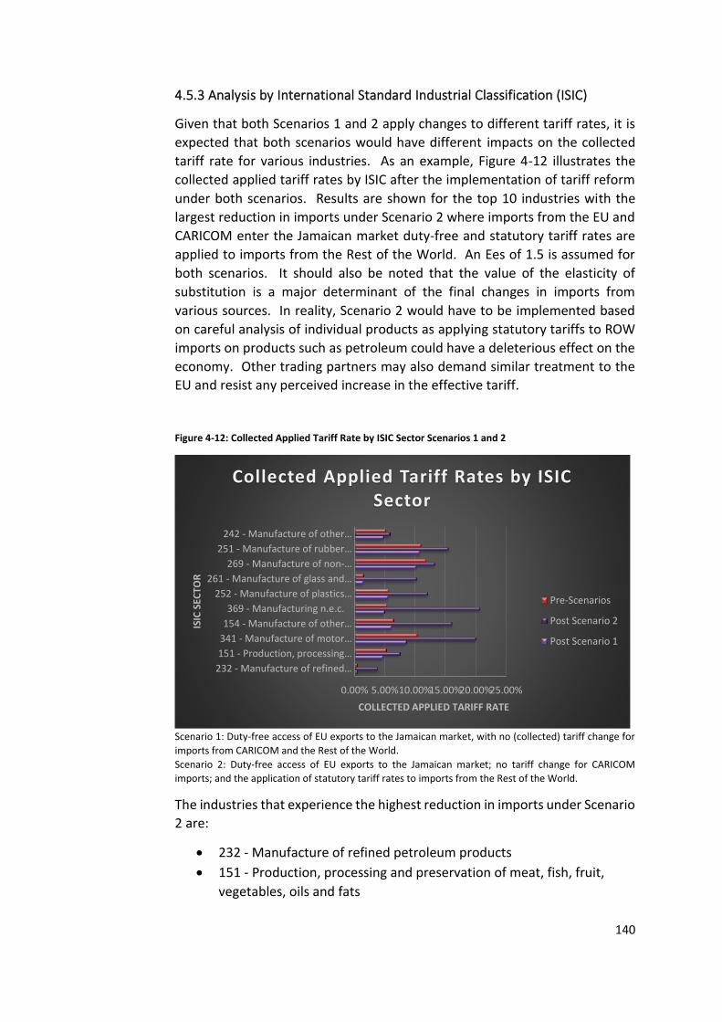
140

4.5.3 Analysis by International Standard Industrial Classification (ISIC)

Given that both Scenarios 1 and 2 apply changes to different tariff rates, it is

expected that both scenarios would have different impacts on the collected

tariff rate for various industries. As an example, Figure 4-12 illustrates the

collected applied tariff rates by ISIC after the implementation of tariff reform

under both scenarios. Results are shown for the top 10 industries with the

largest reduction in imports under Scenario 2 where imports from the EU and

CARICOM enter the Jamaican market duty-free and statutory tariff rates are

applied to imports from the Rest of the World. An Ees of 1.5 is assumed for

both scenarios. It should also be noted that the value of the elasticity of

substitution is a major determinant of the final changes in imports from

various sources. In reality, Scenario 2 would have to be implemented based

on careful analysis of individual products as applying statutory tariffs to ROW

imports on products such as petroleum could have a deleterious effect on the

economy. Other trading partners may also demand similar treatment to the

EU and resist any perceived increase in the effective tariff.

Figure 4-12: Collected Applied Tariff Rate by ISIC Sector Scenarios 1 and 2

Scenario 1: Duty-free access of EU exports to the Jamaican market, with no (collected) tariff change for

imports from CARICOM and the Rest of the World.

Scenario 2: Duty-free access of EU exports to the Jamaican market; no tariff change for CARICOM

imports; and the application of statutory tariff rates to imports from the Rest of the World.

The industries that experience the highest reduction in imports under Scenario

2 are:

• 232 - Manufacture of refined petroleum products

• 151 - Production, processing and preservation of meat, fish, fruit,

vegetables, oils and fats

0.00% 5.00%10.00%15.00%20.00%25.00%

232 - Manufacture of refined…

151 - Production, processing…

341 - Manufacture of motor…

154 - Manufacture of other…

369 - Manufacturing n.e.c.

252 - Manufacture of plastics…

261 - Manufacture of glass and…

269 - Manufacture of non-…

251 - Manufacture of rubber…

242 - Manufacture of other…

COLLECTED APPLIED TARIFF RATE

ISIC

SEC

TOR

Collected Applied Tariff Rates by ISIC Sector

Pre-Scenarios

Post Scenario 2

Post Scenario 1

141

• 341 - Manufacture of motor vehicles

• 154 - Manufacture of other food products

• 369 - Manufacturing n.e.c.

• 252 - Manufacture of plastics products

• 261 - Manufacture of glass and glass products

• 269 - Manufacture of non-metallic mineral products n.e.c.

• 251 - Manufacture of rubber products

• 242 - Manufacture of other chemical products

In most cases, the collected applied tariff rate more than doubles from its

initial value; for example, the collected applied tariff rate for the manufacture

of refined petroleum products and for the manufacture of motor vehicles

move from 0.46% and 10.40% to 3.87% and 20.09%, respectively (see Table 4-

6). In the case of motor vehicles, imports from the EU increased by over $14

million under scenario 2, with the share of EU imports in total motor vehicle

imports increasing from 17.3% pre-reform to 24% post-reform. It should also

be noted that, as TRIST does not estimate changes for tariff lines with an initial

value of zero, where there are no initial imports from the EU in a particular

tariff line, the demand effect is especially strong as consumers face higher

prices to purchase the same goods due to the application of statutory tariff

rates.

In contrast, the change in the collected applied tariff rate is much lower under

Scenario 1. For petroleum products and motor vehicle industries, the collected

applied tariff rates move from the initial levels of 0.46% and 10.4% to 0.45%

and 8.58%, respectively. Both scenarios therefore yield very different trade

diversion and trade creation effects and consequently, varied net welfare

effects. For Scenario 1, the Top 10 industries with the largest increases in

import value are:

• 341 - Manufacture of motor vehicles

• 155 - Manufacture of beverages

• 151 - Production, processing and preservation of meat, fish, fruit,

vegetables, oils and fats

• 011 - Growing of crops; market gardening; horticulture

• 242 - Manufacture of other chemical products

• 269 - Manufacture of non-metallic mineral products n.e.c.

• 152 - Manufacture of dairy products

• 154 - Manufacture of other food products

• 343 - Manufacture of parts and accessories for motor vehicles and

their engines

• 101 - Mining and agglomeration of hard coal

142

Table 4-7 shows the changes in the collected applied tariff rate for these

industries under both scenarios at an Ees of 1.5. In the case of scenario 1,

these rates are reduced and this has a positive overall effect on demand and

consequently increases imports from these industries. In the case of motor

vehicle imports, the share of imports from the EU increases from 17.3% to 19%

- less than the increase observed under Scenario 2. Motor vehicle imports

from the EU increase by over $7.3 million while ROW imports of motor vehicles

fall by approximately $800,000. This is not surprising as the lower change in

tariffs on ROW imports means that there is less source substitution and

consequently, only a minor reduction in ROW motor vehicle imports.

143

Table 4-6: Top 10 Industries by Imports Value Change for Scenario 1 RESULTS BY ISIC SECTOR

Protection (Collected applied tariff rate) Price Change for Imports Initial Value of Value Change

% Change in imports

ISIC Initial Rates Post Scenario 1 Post Scenario 2 Scenario 1 Scenario 2 Imports Scenario 1 Scenario 2 Scenario 1 Scenario 2

341 - Manufacture of motor vehicles

10.40% 8.58% 20.09% -1.56% 10.67% 351,471,551 6,566,486 -45,990,003 1.87% -13.08%

155 - Manufacture of beverages 4.30% 3.03% 1.92% -1.15% -2.10% 198,669,622 3,485,620 5,643,207 1.75% 2.84%

151 - Production, processing and preservation of meat, fish, fruit, vegetables, oils and fats

5.27% 4.72% 7.54% -0.48% 4.25% 365,045,414 2,434,779 -50,218,001 0.67% -13.76%

011 - Growing of crops; market gardening; horticulture

3.54% 2.33% 3.01% -0.99% 0.01% 194,933,187 2,227,563 -1,670,690 1.14% -0.86%

242 - Manufacture of other chemical products

5.18% 4.83% 5.86% -0.31% 0.81% 297,990,725 1,040,387 -3,710,465 0.35% -1.25%

269 - Manufacture of non-metallic mineral products n.e.c.

11.85% 10.21% 13.30% -1.34% 1.83% 73,528,592 1,024,782 -5,868,754 1.39% -7.98%

152 - Manufacture of dairy products

6.71% 5.27% 10.73% -1.26% 4.59% 57,341,256 926,671 -2,601,924 1.62% -4.54%

154 - Manufacture of other food products

6.48% 6.12% 16.12% -0.31% 10.84% 221,741,816 751,089 -39,203,217 0.34% -17.68%

343 - Manufacture of parts and accessories for motor vehicles and their engines

10.79% 9.84% 10.08% -0.78% -0.55% 59,781,915 624,243 450,419 1.04% 0.75%

101 - Mining and agglomeration of hard coal

4.99% 0.00% 0.01% -4.76% -4.75% 7,459,043 319,202 318,853 4.28% 4.27%

144

Table 4-7: Top 10 Industries by Imports Value Change for Scenario 2

RESULTS BY ISIC SECTOR

Protection (Collected applied tariff rate) Price Change for Imports Initial Value of Value Change

% Change in imports

ISIC Initial Rates Post Scenario 1 Post Scenario 2 Scenario 1 Scenario 2 Imports Scenario 1 Scenario 2 Scenario 1 Scenario 2

232 - Manufacture of refined petroleum products

0.46% 0.45% 3.87% -0.01% 3.60% 1,347,858,663 214,137 -125,683,773 0.02% -9.32%

151 - Production, processing and preservation of meat, fish, fruit, vegetables, oils and fats

5.27% 4.72% 7.54% -0.48% 4.25% 365,045,414 2,434,779 -50,218,001 0.67% -13.76%

341 - Manufacture of motor vehicles

10.40% 8.58% 20.09% -1.56% 10.67% 351,471,551 6,566,486 -45,990,003 1.87% -13.08%

154 - Manufacture of other food products

6.48% 6.12% 16.12% -0.31% 10.84% 221,741,816 751,089 -39,203,217 0.34% -17.68%

369 - Manufacturing n.e.c.

5.37% 4.98% 20.75% -0.33% 20.69% 73,638,004 79,813 -28,219,927 0.11% -38.32%

252 - Manufacture of plastics products

5.66% 5.52% 12.13% -0.13% 6.30% 129,883,222 197,448 -10,666,467 0.15% -8.21%

261 - Manufacture of glass and glass products

1.51% 1.46% 10.34% -0.05% 9.08% 48,459,700 30,618 -6,864,365 0.06% -14.17%

269 - Manufacture of non-metallic mineral products n.e.c.

11.85% 10.21% 13.30% -1.34% 1.83% 73,528,592 1,024,782 -5,868,754 1.39% -7.98%

251 - Manufacture of rubber products

11.01% 10.78% 15.52% -0.19% 4.20% 72,973,826 159,077 -3,836,731 0.22% -5.26%

242 - Manufacture of other chemical products

5.18% 4.83% 5.86% -0.31% 0.81% 297,990,725 1,040,387 -3,710,465 0.35% -1.25%

145

4.5.4. Scenario 1 Summary Results by Product

It would be useful to examine Scenario 1 in more detail in order to set a basis

for examining alternative scenarios of tariff reform that may increase revenue

while enhancing welfare at the same time. It should be recalled that in

Scenario 1, the “all duty free” option is selected for the EU and “no tariff

change” for CARICOM and the Rest of the World (ROW). The elasticity of

export substitution is estimated at 1.5; the elasticity of domestic substitution

at 1, and the elasticities of demand are Kee et al. (2008) estimates for Jamaican

imports. The TRIST simulation estimates that under this scenario imports will

increase by 0.4% or US$22.6 million as a result of full liberalization under the

EU-EPA. Revenue loss is estimated at 9% for collected tariff and 2.4% for total

taxes on imports (includes the General Consumption Tax, Additional Stamp

Duty and other duties) from the pre EPA full liberalization level. With respect

to the net welfare effect, the simulation showed a small net welfare loss of -

$42,796 at an elasticity of export substitution value of 1.5. The sensitivity

analysis showed that the net welfare effect is small and positive in the case of

Ees = 1 and negative in the case of Ees = 2 at a value of (-$103,395), which led

to the conclusion that the Ees value had a very strong effect on the trade

diversion estimate as diversion increased substantially as the Ees value was

raised. It would appear that at lower Ees values, the EPA would result in less

consumers switching from ROW to EU suppliers.

Table 4-8: Average Collected Applied Rates

Average Collected Applied Tariff Rates

Pre Scenario 1

Post Scenario 1

Import Weighted Average Collected Applied Tariff Rate

3.6% 3.3%

Import Weighted Average ROW Collected Applied Tariff Rate

4.284% 4.281%

Simple ROW Average Collected Applied Rate 7.43265% 7.43121% Scenario 1: Duty-free access of EU exports to the Jamaican market, with no (collected) tariff change for

imports from CARICOM and the Rest of the World.

Table 4-8 provides summary statistics on the average import weighted applied

tariff for imports in general and ROW imports specifically. It shows that the

average collected applied tariff rate (weighted by imports) declines by 9.4% as

a result of full trade liberalisation of EU products. The average applied tariff

for ROW imports declines marginally from 4.284% to 4.281%. In real terms,

while total imports increase by $22.6 million after full liberalisation of EU

imports under the EPA, ROW imports decline by -$1.9 million. This explains

the marginal change in the import weighted average ROW collected applied

tariff as the change in ROW imports is relatively small. However, the change

146

in revenue is much greater. Under this scenario, collected applied tariff

revenue declines by $20.3 million and total fiscal revenue (tariff revenue plus

value added taxes, and stamp duties, etc.) declines by $19 million.

In order to assess the main products that would generate the revenue loss,

Table 4-9 lists the Top 25 tariff lines with the highest revenue loss (see

Appendix 4A for tariff line descriptions). These 25 lines constitute 59% of the

total loss in collected applied tariff revenue and 61% of the loss in ROW tariff

revenue. Of the 25 lines, 10 are related to motor vehicle imports of varying

engine sizes. The product with the highest revenue loss is onions. Motor

vehicles of engine size between 2000cc and 3000cc; other potatoes, prepared

or preserved; tiles, cubes, etc; and Motor vehicles of engine size between

2500cc and 3200cc round out the Top 5. For these products, the net welfare

loss/gain varies. For example, although onions have the highest revenue loss

for any tariff line, there is a small welfare gain as a result of full liberalisation

with the EU under an EPA.

Like other free trade agreements, trade liberalisation is considered to take

place within the trade agreement once substantially all trade is not subject to

import duties (see Article 24 of the General Agreement on Tariffs and Trade

1994). In practice, for the EPA, ‘substantially all trade’ has been interpreted to

mean that at least 80% of trade in goods between CARICOM and the EU would

have to be liberalized. Table 4-10 provides the share of these top 25 tariff lines

in total EU imports. In order to avoid negative revenue effects, Jamaica may

simply exclude the majority of these lines from import liberalisation as their

exclusion would still mean that substantially all trade has been liberalized. If

the condition used is 20% of EU trade before the tariff reform scenario is

implemented, then 21 out of the 25 products could be excluded as they

comprise 19% of total EU imports into Jamaica. If the condition is 20% post-

scenario, then 19 of these lines could be excluded, comprising 20% of total EU

imports. It would be therefore instructive to compare these results with the

actual end term EU-CARIFORUM EPA that was negotiated with excluded

products.

147

Table 4-9: Top 25 Tariff lines by Revenue Loss with Change in Imports and Welfare (US$)

Tariff Line ROW Post collected applied tariff

Change in Collected Applied Tariff Revenue (US$)

Change in Collected Applied Tariff Revenue from ROW Imports (US$)

Change in Total Fiscal Revenue (US$)

Change in Total Fiscal Revenue from ROW Imports (US$)

Total Change in Imports (US$)

Change in Imports from ROW (US$)

NET WELFARE LOSS/GAIN (US$)

Total -20,264,307 -256,600 -19,022,713 -622,762 22,644,920 -1,862,552 -42,796

0703101000 35.8% -1,616,022 1,089 -1,562,488 2,450 1,766,240 3,045 23,915

8703234030 8.2% -1,245,245 -16,054 -1,088,750 -58,484 1,416,168 -194,600 -11,219

2004109000 18.3% -1,073,052 -15,663 -1,064,370 -38,354 1,115,259 -85,775 2,250

6908901000 17.9% -925,794 -42,613 -948,134 -100,073 813,958 -237,630 -11,347

8703339030 10.3% -911,467 -14,559 -831,948 -44,710 926,348 -140,909 -1,560

8703233030 10.5% -887,791 -16,533 -823,399 -49,590 1,009,035 -156,809 -12,640

0701900000 40.0% -657,645 -19,132 -657,661 -19,148 426,827 -47,838 3,634

2202909030 20.0% -654,169 8,669 -473,863 29,943 1,095,390 43,344 10,830

2204100010 28.4% -477,708 -16,385 -504,596 -65,708 432,384 -57,634 -1,112

8703232031 12.4% -389,798 -6,998 -350,777 -21,121 434,668 -56,651 -3,748

2701190000 5.0% -372,402 -1 -384,372 -6 319,202 -21 5,265

8703322031 10.0% -289,262 -251 -274,088 -646 346,855 -2,520 5,129

0402210010 0.0% -278,521 0 -278,521 0 317,057 -2,410 2,820

2208700020 11.7% -226,193 193 -203,105 592 297,421 1,653 2,692

8703234010 20.6% -219,463 -5,125 -177,125 -7,509 235,835 -24,912 -3,144

2005519000 16.6% -202,296 7,550 -151,801 17,910 433,603 45,386 4,111

8703249032 15.9% -197,737 187 -138,589 851 274,620 1,177 2,256

8418300000 19.5% -184,821 -5,945 -186,308 -13,970 177,517 -30,414 -1,440

8703233011 17.0% -181,066 -3,602 -171,504 -3,707 195,756 -21,235 -2,568

2208201020 0.9% -168,588 192 -101,414 1,996 433,916 21,536 5,982

8703339011 16.4% -166,800 -4,643 -143,684 -6,832 160,679 -28,281 -1,673

2106909010 17.8% -164,587 -5,322 -172,060 -12,687 142,141 -29,882 386

8703232030 13.3% -158,822 -3,717 -158,371 -9,737 182,550 -27,938 -1,515

1904100000 18.7% -156,050 -3,147 -159,115 -7,633 142,420 -16,796 932

2004909000 20.0% -154,524 5,600 -126,573 13,160 278,760 28,007 1,784

148

Table 4-10: Proportion of EU imports in each tariff line in total EU imports Pre and Post Scenario 1

Tariff Line Change in Collected Applied Tariff Revenue (US$)

Pre-Scenario 1 Proportion of Tariff line Imports in total EU Imports

Pre-Scenario 1 Cumulative Proportion

Post-Scenario 1 Proportion of Tariff line in total EU Imports

Post-Scenario 1 Cumulative Proportion

0703101000 -1,616,022 0.93% 0.93% 1.26% 1.26%

8703234030 -1,245,245 3.49% 4.42% 3.65% 4.91%

2004109000 -1,073,052 1.26% 5.67% 1.45% 6.36%

6908901000 -925,794 1.11% 6.78% 1.28% 7.64%

8703339030 -911,467 2.02% 8.80% 2.14% 9.78%

8703233030 -887,791 2.35% 11.15% 2.48% 12.26%

0701900000 -657,645 0.37% 11.51% 0.45% 12.71%

2202909030 -654,169 1.43% 12.94% 1.58% 14.29%

2204100010 -477,708 0.39% 13.33% 0.48% 14.77%

8703232031 -389,798 0.78% 14.11% 0.84% 15.61%

2701190000 -372,402 1.71% 15.82% 1.69% 17.30%

8703322031 -289,262 0.77% 16.59% 0.80% 18.10%

0402210010 -278,521 0.23% 16.82% 0.29% 18.39%

2208700020 -226,193 0.30% 17.12% 0.35% 18.74%

8703234010 -219,463 0.23% 17.35% 0.28% 19.02%

2005519000 -202,296 0.24% 17.59% 0.31% 19.33%

8703249032 -197,737 0.46% 18.05% 0.49% 19.82%

8418300000 -184,821 0.21% 18.25% 0.24% 20.06%

8703233011 -181,066 0.20% 18.45% 0.24% 20.29%

2208201020 -168,588 0.40% 18.85% 0.47% 20.76%

8703339011 -166,800 0.17% 19.02% 0.20% 20.96%

2106909010 -164,587 3.34% 22.36% 3.20% 24.16%

8703232030 -158,822 0.91% 23.27% 0.91% 25.07%

1904100000 -156,050 0.18% 23.45% 0.21% 25.28%

2004909000 -154,524 0.18% 23.63% 0.23% 25.51%

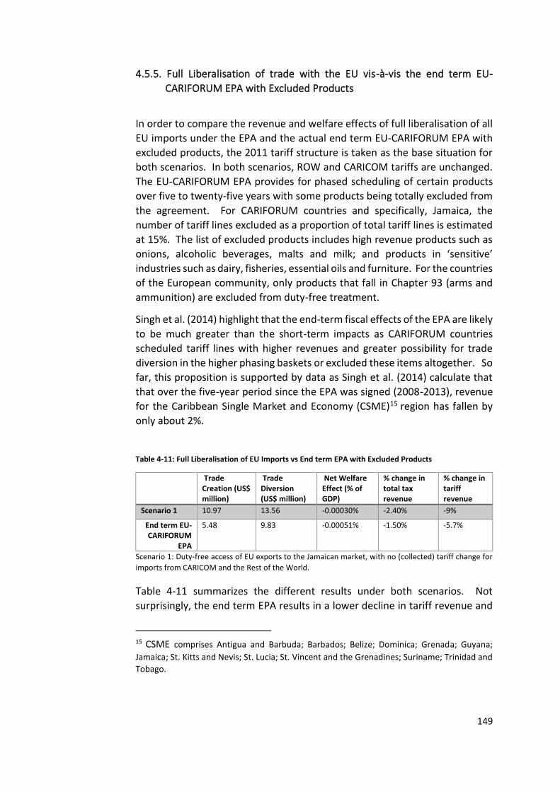
149

4.5.5. Full Liberalisation of trade with the EU vis-à-vis the end term EU-

CARIFORUM EPA with Excluded Products

In order to compare the revenue and welfare effects of full liberalisation of all

EU imports under the EPA and the actual end term EU-CARIFORUM EPA with

excluded products, the 2011 tariff structure is taken as the base situation for

both scenarios. In both scenarios, ROW and CARICOM tariffs are unchanged.

The EU-CARIFORUM EPA provides for phased scheduling of certain products

over five to twenty-five years with some products being totally excluded from

the agreement. For CARIFORUM countries and specifically, Jamaica, the

number of tariff lines excluded as a proportion of total tariff lines is estimated

at 15%. The list of excluded products includes high revenue products such as

onions, alcoholic beverages, malts and milk; and products in ‘sensitive’

industries such as dairy, fisheries, essential oils and furniture. For the countries

of the European community, only products that fall in Chapter 93 (arms and

ammunition) are excluded from duty-free treatment.

Singh et al. (2014) highlight that the end-term fiscal effects of the EPA are likely

to be much greater than the short-term impacts as CARIFORUM countries

scheduled tariff lines with higher revenues and greater possibility for trade

diversion in the higher phasing baskets or excluded these items altogether. So

far, this proposition is supported by data as Singh et al. (2014) calculate that

that over the five-year period since the EPA was signed (2008-2013), revenue

for the Caribbean Single Market and Economy (CSME)15 region has fallen by

only about 2%.

Table 4-11: Full Liberalisation of EU Imports vs End term EPA with Excluded Products

Trade Creation (US$ million)

Trade Diversion (US$ million)

Net Welfare Effect (% of GDP)

% change in total tax revenue

% change in tariff revenue

Scenario 1 10.97 13.56 -0.00030% -2.40% -9%

End term EU-CARIFORUM

EPA

5.48 9.83 -0.00051% -1.50% -5.7%

Scenario 1: Duty-free access of EU exports to the Jamaican market, with no (collected) tariff change for

imports from CARICOM and the Rest of the World.

Table 4-11 summarizes the different results under both scenarios. Not

surprisingly, the end term EPA results in a lower decline in tariff revenue and

15 CSME comprises Antigua and Barbuda; Barbados; Belize; Dominica; Grenada; Guyana;

Jamaica; St. Kitts and Nevis; St. Lucia; St. Vincent and the Grenadines; Suriname; Trinidad and

Tobago.

150

total tax revenue when compared with the full liberalisation of EU imports into

Jamaica. The 5.7% decline in tariff revenue is not as high as the 12% decline

estimated for Jamaica under the EPA by Busse and Lüehje (2007). In absolute

terms, the model estimates a lower reduction in tariff revenue of $12.8 million

for the End-term EU-CARIFORUM EPA than those estimated by Stevens et al.

(2009) for the Overseas Development Institute (€26.8 million or $39.5 million)

and Fontagné et al. (2009) for CEPII (€14.1 million or $20.7 million).

Additionally, trade creation and trade diversion levels are less for the end term

EPA than under full liberalisation of EU imports. This is expected given that full

liberalisation removes duties on all EU imports thereby increasing the potential

for trade diversion from ROW products and increasing opportunities for trade

creation by diverting more expensive imports from ROW and CARICOM

producers to more efficient EU producers. It should also be noted that the

welfare loss is greater for the end term EPA; however, both levels are less than

one-thousandth of a percent of Jamaica’s 2011 GDP. The reduction in welfare

is much lower than the 4.5% welfare loss estimated for Jamaica by Greenaway

and Milner (2006) in the case where CARICOM grants reciprocal market access

to the EU only (EU reciprocity case). Indeed, since the signing of the EPA in

2008, the global financial crisis of 2007/8 and inadequate initial trade links

between CARIFORUM and the European Union have meant that some of the

projected benefits and costs of the EPA have not materialised. Singh et al.

(2014) note that, in 2012, imports from the EU for Jamaica had fallen back to

close to 2004 levels. It is clear therefore that in line with Ambassador

Amedi’s16 comments, there are other factors that influence competitiveness

and market penetration besides market access.

While the approach outlined above is useful and expedient for policy purposes,

a more holistic approach to tariff reform is recommended, which might

generate both positive changes in revenue and welfare. In addition, where

welfare and revenue concerns intersect, the issue is often posed as a trade-off

– increased tariff revenue often means lower welfare and vice versa. The next

section also explores whether this is necessarily the case. Indeed, it may not

be possible to achieve both and the final decision will be made by policymakers

based on their judgement of what is most appropriate for their economies at

a given point in time.

16 “EU Laments Jamaica's Failure To Maximise EPA Benefits”, Jamaica Gleaner, 23

October 2014

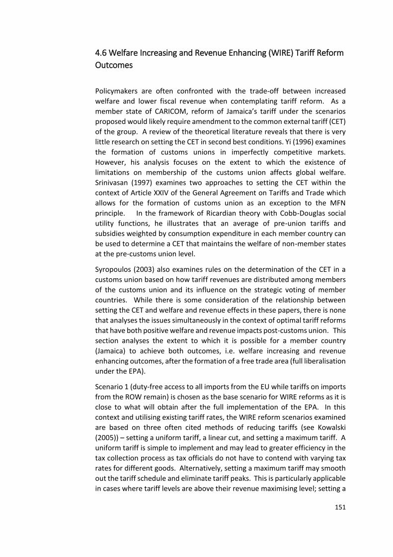
151

4.6 Welfare Increasing and Revenue Enhancing (WIRE) Tariff Reform

Outcomes

Policymakers are often confronted with the trade-off between increased

welfare and lower fiscal revenue when contemplating tariff reform. As a

member state of CARICOM, reform of Jamaica’s tariff under the scenarios

proposed would likely require amendment to the common external tariff (CET)

of the group. A review of the theoretical literature reveals that there is very

little research on setting the CET in second best conditions. Yi (1996) examines

the formation of customs unions in imperfectly competitive markets.

However, his analysis focuses on the extent to which the existence of

limitations on membership of the customs union affects global welfare.

Srinivasan (1997) examines two approaches to setting the CET within the

context of Article XXIV of the General Agreement on Tariffs and Trade which

allows for the formation of customs union as an exception to the MFN

principle. In the framework of Ricardian theory with Cobb-Douglas social

utility functions, he illustrates that an average of pre-union tariffs and

subsidies weighted by consumption expenditure in each member country can

be used to determine a CET that maintains the welfare of non-member states

at the pre-customs union level.

Syropoulos (2003) also examines rules on the determination of the CET in a

customs union based on how tariff revenues are distributed among members

of the customs union and its influence on the strategic voting of member

countries. While there is some consideration of the relationship between

setting the CET and welfare and revenue effects in these papers, there is none

that analyses the issues simultaneously in the context of optimal tariff reforms

that have both positive welfare and revenue impacts post-customs union. This

section analyses the extent to which it is possible for a member country

(Jamaica) to achieve both outcomes, i.e. welfare increasing and revenue

enhancing outcomes, after the formation of a free trade area (full liberalisation

under the EPA).

Scenario 1 (duty-free access to all imports from the EU while tariffs on imports

from the ROW remain) is chosen as the base scenario for WIRE reforms as it is

close to what will obtain after the full implementation of the EPA. In this

context and utilising existing tariff rates, the WIRE reform scenarios examined

are based on three often cited methods of reducing tariffs (see Kowalski

(2005)) – setting a uniform tariff, a linear cut, and setting a maximum tariff. A

uniform tariff is simple to implement and may lead to greater efficiency in the

tax collection process as tax officials do not have to contend with varying tax

rates for different goods. Alternatively, setting a maximum tariff may smooth

out the tariff schedule and eliminate tariff peaks. This is particularly applicable

in cases where tariff levels are above their revenue maximising level; setting a

152

maximum tariff level that is below this level may in fact increase tariff revenue

and welfare. Finally, a linear cut is one of the most frequently used methods

for reducing tariff rates. Falvey and Kim (1992) note a general rule that a

proportional reduction in all tariffs raises welfare. In order to select

appropriate values for the three scenarios, different values were utilised in

TRIST to illustrate the possibilities of WIRE reforms empirically. After reviewing

the results of the simulations, the ones presented here are judged to be the

most appropriate for the dataset and scenarios. From the outset, it should be

noted that as a member of CARICOM, Jamaica implements the CET, with some

derogations. In presenting these scenarios, it is understood that Jamaica

would need to seek derogations or amendments to the CET from

CARICOM/COTED to give effect to some of these proposals.

Taking Scenario 1 (duty-free access to all imports from the EU while tariffs on

imports from the ROW remain) as the initial scenario, the three additional

scenarios are:

I. Scenario 3 – A linear cut of a) 5% and b) 10% on ROW duties, with

duties on imports from the EU and CARICOM being duty-free provided

that they meet the rules of origin.

II. Scenario 4 – A maximum tariff of a) 15% and b) 20% c) 30% and d)

32% applied to ROW imports, with duties on imports from the EU and

CARICOM being duty-free.

III. Scenario 5 – A uniform tariff of a) 7.4% and b) 4.5% c) 4.3% and d)

3.3% applied to ROW imports, with duties on imports from the EU and

CARICOM being duty-free

It is important to frame the results in the context of the existing tariff structure

in order to understand the impacts of each tariff reform scenario. From the

data analysis section, Jamaica’s simple average tariff in 2011 for agricultural

products was 17.9% and 6% for non-agricultural products. Forty-one percent

of agricultural products in 2011 had duty-free status while a further 46% had

applied rates of between 15% and 50%. Duty-free treatment was applied to

70% of non-agricultural tariff lines and 27% had applied rates of between 0%-

25%. The highest applied MFN tariff rates were found on: Fish and fish

products (28.8%); animal products (26.5%); dairy products (25.2%); fruits,

vegetables, plants (23%); and beverages and tobacco (23%). The lowest

applied MFN rates were found on imports of cotton (0%); non-electrical

machinery (1.5%); and chemicals (2.6%). Petroleum products and chemicals

constituted the larger share of imports valuing 27.3% (40.4% duty-free) and

13% (64.2% duty-free), respectively.

153

Figure 4-10: Comparison of Initial Applied Tariff Rates and Statutory Tariff Rates

Figure 4-13 shows the variation between the collected applied tariff rate and

the statutory tariff rate, that is, the difference in what is authorised (the

statutory rate) and what is in fact collected by the tax authorities (the initial

applied tariff rate) after full liberalisation of EU imports under the EU-

CARIFORUM EPA, with ROW and CARICOM tariffs unchanged. While a

statutory tariff rate of less than 10% applies to 60% of all tariff lines, a tariff of

less than 10% is collected in 71% of tariff lines. Additionally, a statutory tariff

of between 26% - 50% applies to about 8% of tariff lines; however, tariff rates

of between 26% - 50% were actually collected in only about 4% of tariff lines.

This suggests that there is some revenue loss that occurs through the

discretionary application of the statutory tariff. The analysis of the scenarios

that follow use the collected applied tariff rate as this presents a more realistic

picture of the likely outcome of tariff reform than if the statutory tariff rates

were utilised.

Moving from an initial second-best scenario of full liberalisation with the EU

and CARICOM, and ROW tariffs remaining unchanged, the welfare effects are

positive while there is a small reduction in tariff revenue when the collected

applied tariff rate on ROW imports is reduced by 5% and 10% (Scenarios 3a

and 3b in Table 4-12, respectively). In the case of a 5% reduction, there is a

positive welfare gain of $125,771 and tariff revenue falls by 4%. When the

collected applied tariff rate is reduced by 10% (as shown in Figure 4-14), the

welfare gain is almost double the amount observed at a 5% reduction, valuing

$246,385. Tariff revenue also falls by 8%. Thus, under this scenario, as the

rate of reduction increases, tariff revenue falls but welfare gains increase.

0.0%

10.0%

20.0%

30.0%

40.0%

50.0%

60.0%

70.0%

0%-5% 6% - 10% 11% - 15% 16% - 25% 26% - 50% 51% - 100%Per

cen

tage

of

Tari

ff L

ines

Tariff Rates

Comparison of Initial Applied Tariff Rates and Statutory Tariff Rates

Scen 1 Initial Applied Tariff Rate Scen 1 Statutory Tariff Rate

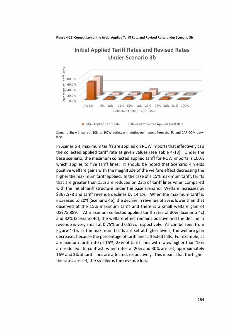
154

Figure 4-11: Comparison of the Initial Applied Tariff Rate and Revised Rates under Scenario 3b

Scenario 3b: A linear cut 10% on ROW duties, with duties on imports from the EU and CARICOM duty-free.

In Scenario 4, maximum tariffs are applied on ROW imports that effectively cap

the collected applied tariff rate at given values (see Table 4-13). Under the

base scenario, the maximum collected applied tariff for ROW imports is 100%

which applies to five tariff lines. It should be noted that Scenario 4 yields

positive welfare gains with the magnitude of the welfare effect decreasing the

higher the maximum tariff applied. In the case of a 15% maximum tariff, tariffs

that are greater than 15% are reduced on 23% of tariff lines when compared

with the initial tariff structure under the base scenario. Welfare increases by

$367,578 and tariff revenue declines by 14.1%. When the maximum tariff is

increased to 20% (Scenario 4b), the decline in revenue of 3% is lower than that

observed at the 15% maximum tariff and there is a small welfare gain of

US$75,889. At maximum collected applied tariff rates of 30% (Scenario 4c)

and 32% (Scenario 4d), the welfare effect remains positive and the decline in

revenue is very small at 0.75% and 0.55%, respectively. As can be seen from

Figure 4-15, as the maximum tariffs are set at higher levels, the welfare gain

decreases because the percentage of tariff lines affected falls. For example, at

a maximum tariff rate of 15%, 23% of tariff lines with rates higher than 15%

are reduced. In contrast, when rates of 20% and 30% are set, approximately

16% and 3% of tariff lines are affected, respectively. This means that the higher

the rates are set, the smaller is the revenue loss.

0.0%

20.0%

40.0%

60.0%

80.0%

0%-5% 6% - 10% 11% - 15% 16% - 25% 26% - 50% 51% - 100%

Per

cen

tage

of

Tari

ff L

ines

Collected Applied Tariff Rates

Initial Applied Tariff Rates and Revised Rates Under Scenario 3b

Initial Applied Tariff Rate Revised Collected Applied Tariff Rate

155

Figure 4-12: Initial Applied Tariff Rates and Maximum Rates under Scenario 4

Scenario 4: Maximum tariffs are applied on ROW imports that cap the collected applied tariff rate at 20% (4b) and 30% (4c)

Scenario 5 examines the effect of applying a uniform tariff on ROW imports

after full liberalisation of imports from the EU and CARICOM. In Scenario 5a,

where the simple average collected applied tariff of 7.4% is set as a uniform

tariff, there is an increase in tariff revenue of 37.6%; however, there is a net

welfare loss of -US$835,660 (see Table 4-14). This net welfare loss should be

anticipated as a uniform tariff of 7.4% increases the tariff rate on

approximately 65% of tariff lines that previously had tariff rates below 7.4%

under the initial scenario (see Figure 4-16). When the uniform tariff rate is

lowered, it is expected that there will be a reduction in the net welfare loss

and also a decrease in tariff revenue. This is observed in Scenario 5b where

the uniform tariff is set at 4.5% and the net welfare loss is now -US$110,978.

It should be noted that in this case, however, the new tariff revenue is above

the initial level by US$6.8 million. Scenario 5c utilizes the import weighted

ROW collected applied tariff rate of 4.3% while Scenario 5d applies the import

weighted collected applied tariff rate from all sources of 3.3%. In comparison

to applying the simple average collected applied tariff rate of 7.4%, the welfare

loss is significantly less when the import weighted average tariff is used –

US$886,818 in the case of the former compared to US$70,549 and US$23,895

when the import weighted ROW and all source average tariffs are used,

respectively. In all cases, there is a decline in total imports, with the smallest

decline and lowest welfare loss in the case of Scenario 5d. This is expected as

Scenario 5d applies the lowest uniform tariff. However, as the welfare loss

decreases with the reduction in the uniform tariff, the revenue loss increases.

This is illustrated by the variation in the change in revenue between Scenario

5a and Scenario 5d where there is an increase in tariff revenue of 62% when

0.0%

10.0%

20.0%

30.0%

40.0%

50.0%

60.0%

70.0%

0%-5% 6% - 10% 11% - 15% 16% - 25% 26% - 30% 31% - 50% 51%-100%

Initial Applied Tariff Rates and Maximum Rates under Scenario 4

Initial Applied Tariff Rate Scenario 4c Scenario 4b

156

the simple average tariff of 7.4% is used compared to 23% reduction in tariff

revenue when the import weighted average of 3.3% is applied.

Figure 4-13: Applying a uniform tariff rate to the collected tariff rate structure

It should be noted that all uniform tariff scenarios lead to welfare losses while

both linear cut scenarios and maximum tariff scenarios see positive changes in

welfare. At lower levels of the maximum tariff, higher welfare values are

observed; however, they are associated with lower tariff revenues. Based on

the results of the various scenarios, it may be said that there are certain

conditions that increase the likelihood of WIRE reforms. Of all the scenarios,

Scenario 4d seems the most likely to yield a WIRE reform. After applying a

maximum tariff of 32%, there is a welfare gain of $15,128.42 and there is a fall

in revenue of 0.55% that could be seen as a neutral effect. The results of the

various scenarios suggest that the pre-existing tariff structure is a major

determinant of a WIRE reform outcome. Countries with high tariffs and large

variations between tariffs are more likely to have positive welfare effects as a

result of tariff reform and especially in the case where a uniform tariff is

applied, may see an increase in tariff revenue, depending on the assumptions

relating to the elasticities of demand, and exporter substitution.

0.0%

10.0%

20.0%

30.0%

40.0%

50.0%

60.0%

70.0%

0%-5% 6% - 10% 11% - 15% 16% - 25% 26% - 50% 51% - 100%

Pe

rce

nta

ge o

f ta

riff

lin

es

Collected applied tariff rate

APPLYING UNIFORM TARIFF RATE OF 4 .3% AND 7.4% TO THE COLLEC TED TARIFF RATE

STRUCTURE

Per cent of tariff lines grouped by collected applied tariff rate

Uniform tariff of 7.4%

Uniform tariff of 4.3%

157

Table 4-12: Revenue and Welfare Impacts of Linear Cuts in the Collected Applied Tariff Rate (US$ million)

Total Imports Imports from

the EU Imports from ROW

Imports from CARICOM

Percentage Change in Tariff Revenue

Percentage Change in Total Tax Revenue

Welfare Change (% of GDP)

Scenario 1 (base values) 6,249.06 460.77 4,752.53 1,035.77 204.30 780.93

Post Scenario 3a - Linear cut of 5% in the collected applied tariff rate

6,260.71 460.59 4,764.12 1,036.00 -4.1%

-1.0% 0.00087%

Post Scenario 3b - Linear cut of 10% in the collected applied tariff rate

6,272.46 460.42 4,775.69 1,036.35 -8.3% -2.0% 0.00171%

Table 4-13: Revenue and Welfare Impacts of Maximum Collected Applied Tariff Rates (US$ million)

Total Imports Imports from the EU Imports from ROW Imports from CARICOM

Percentage Change in Tariff Revenue

Percentage Change in Total Tax Revenue

Welfare Change

Scenario 1 (base values) 6,249.06 460.77 4,752.53 1,035.77 204.30 780.93

Post Scenario 4a - Maximum tariff of 15% for the collected applied tariff rate

6,285.85 460.40 4,789.50 1,035.95 -14.1% -3.5% 0.00255%

Post Scenario 4b - Maximum tariff of 20% for the collected applied tariff rate

6,256.43 460.70 4,760.00 1,035.73 -2.9% -0.7% 0.00053%

Post Scenario 4c - Maximum tariff of 30% for the collected applied tariff rate

6,251.06 460.77 4,754.55 1,035.74 -0.7% -0.2% 0.00014%

Post Scenario 4d - Maximum tariff of 32% for the collected applied tariff rate

6,250.56 460.77 4,754.04 $1,035.74 -0.5% -0.1% 0.00010%

158

Table 4-14: Revenue and Welfare Impacts of Uniform Collected Applied Tariff Rates (US$ million)

Total Imports Imports from the EU Imports from

ROW Imports from CARICOM

Percentage Change in Tariff Revenue

Percentage Change in Total Tax Revenue

Welfare Change (% of GDP)

Scenario 1 (base values) 6,249.06 460.77 4,752.53 1,035.77 204.30 780.93

Post Scenario 5a - Uniform tariff of 7.4% applied to Imports from ROW

5,947.14 462.59 4,470.32 1,014.23 62.4% 15.7% -0.00614%

Post Scenario 5b - Uniform tariff of 4.5% applied to Imports from ROW

6,156.68 460.65 4,671.35 1,024.68 3.3% 0.9% -0.00077%

Post Scenario 5c - Uniform tariff of 4.3% applied to Imports from ROW

6,171.19 460.53 4,685.26 1,025.40 -1.0% -0.1% -0.00049%

Post Scenario 5d - Uniform tariff of 3.3% applied to Imports from ROW

6,243.83 459.91 4,754.87 1,029.05 -22.8% -5.6% -0.00017%

159 | P a g e

4.7 Conclusions

This chapter sought to examine different tariff reform scenarios for Jamaica

under the EU-CARIFORUM EPA and analyse the possibility of achieving WIRE

outcomes with tariff liberalisation. The specific aims introduction were to:

I. explore the tariff revenue, trade creating, trade diverting and welfare

effects of full liberalisation under the EU-CARIFORUM EPA at the

product level for Jamaica.

II. examine the different effects of utilising statutory tariff rates versus

collected tariff rates in the analysis

III. analyse how Jamaica may adjust its tariffs on ROW imports after

implementation of the EPA in order to address concerns about tariff

revenue depletion and welfare loss, for example.

IV. examine the feasibility of achieving welfare increasing and revenue

enhancing (WIRE) outcomes for tariff adjustments on ROW imports

post-EPA.

With respect to points (i) and (ii), it is shown that Jamaica can mitigate negative

fiscal effects of the EU-CARIFORUM EPA with the application of statutory tariff

rates rather than collected tariff rates. However, there is a trade-off between

revenue and welfare, as in the case of the application of statutory tariff on

ROW imports, there is a significant increase in total tariff revenue but a net

welfare loss. This essay also showed that the effects of tariff liberalisation

under the EPA vary by industry and product. In particular, where there are no

imports from the EU to replace imports from the ROW, the demand effect is

especially strong as consumers face higher prices to purchase the same goods,

particularly when statutory tariff rates are applied.

With respect to point (iii), in order to mitigate negative revenue effects of tariff

reform, the essay showed that Jamaica may exclude high revenue products

from the EU-CARIFORUM EPA as their exclusion would still mean that

substantially all trade has been liberalized under the GATT definition. For

completeness, the results from the scenario of full liberalisation of EU imports

under the EU-CARIFORUM EPA were compared with the provisions of the end

term EU-CARIFORUM EPA that was signed in October 2008 which excludes

approximately 15% of tariff lines. It was observed that the end term EPA

resulted in a lower decline in tariff revenue and total tax revenue when

compared with the full liberalisation of EU imports into Jamaica. The welfare

loss was also found to be greater for the end term EPA. This finding suggests

that the Jamaican authorities included high revenue products on the list of

excluded products and this reduced the potential revenue loss from the EPA

by 37%.

160 | P a g e

With respect to point (iv), the essay showed that it is challenging to design

WIRE reforms. For Jamaica, applying a maximum tariff of 32% to ROW imports

post-EPA is most likely to yield welfare increasing and revenue enhancing

outcomes. All uniform tariff scenarios post-EPA led to welfare losses while

both linear cut scenarios and maximum tariff scenarios post-EPA see positive

changes in welfare. The results also suggest that the pre-existing tariff

structure is a major determinant of a WIRE reform outcome; that is, where

countries have high tariffs and large dispersion between tariffs, they are more

likely to observe positive welfare effects as a result of tariff reform and

particularly where a uniform tariff is applied, may see an increase in tariff

revenue. It should be noted that Jamaica would have to seek derogations or

amendments to the CET from COTED/CARICOM for changes in statutory tariff

rates that are outside of the CET.

This essay has enriched the economic literature on tariff reform and the effects

that it may have on welfare and fiscal revenue. While much of the theoretical

literature on WIRE reforms is established in a first-best framework of non-

preferential liberalisation, this essay explores these effects in the second-best

context of the EU-CARIFORUM EPA, using an empirical approach and is a useful

addition to the literature on WIRE reforms. In a first-best scenario, one can

see that it is easier to establish clearer rules for achieving WIRE outcomes

(Falvey (1994)). In the second-best context, it is not clear that lowering the

tariff is necessarily welfare raising, particularly where the free trade agreement

creates trade diversion. Ultimately, there may not need to be a choice

between welfare and revenue as in the end, policymakers will make a decision

based on their judgement of the needs of their economies.

The essay is also of direct relevance to policymakers in Jamaica and the wider

CARICOM region. It offers a detailed analysis of multiple liberalisation

scenarios, utilising statutory vs. applied tariff rates on ROW imports post-EPA,

which may be used to inform future policy decisions on tariff reform. As

Jamaica has already made provision for high revenue products in its schedule

of commitments under the EPA by placing those items in the later phases of

the agreement, the application of statutory rates, that is, limiting the number

of discretionary waivers and exemptions is one relatively easy way of

increasing tariff revenue. The research will also prove useful for those ACP

regions that have not yet negotiated a final EPA agreement with the EU by

highlighting the possible effects on fiscal revenue and welfare and how they

may be mitigated, in the event that these effects are likely to be negative.

As with all partial equilibrium models, the findings of this essay are limited to

impact effects that do not take into account changes in relative prices and

income due to changes in tariff rates. This provides an opportunity for future

research on economy-wide implications of tariff reform for countries such as

Jamaica, in the context free trade agreements, using a computable general

161 | P a g e

equilibrium model, for example. In addition, there is scope for further

research on WIRE reforms for larger, more developed countries in a similar

second-best environment of a free trade agreement.

162 | P a g e

APPENDIX 4A – TARIFF LINE DESCRIPTIONS

Tariff Line Description

0703101000 Onions

8703234030 Motor vehicle exceeding 2000cc but not exceeding 3000cc imported by dealers (petrol)

2004109000 Other Potatoes [Prepared or Preserved (Frozen; Excluding By Vinegar, Acetic Acid)]

6908901000 Tiles, cubes and similar articles the largest surface of which is capable of being enclosed in a square the side of which is 7 cm or more

8703339030 Motor vehicles 2500cc to 3200cc imported by dealers

8703233030 Motor Vehicle exceeding 1800cc but not exceeding 2000cc imported by Dealers (petrol)

0701900000 Other [Other Potatoes (Fresh or Chilled)]

2202909030 Red Bull, Arizona, Monster and similar energy drinks.

2204100010 Sparkling wine of fresh grapes.

8703232031 Motor vehicle exceeding 1600cc but not exceeding 1800cc imported by dealers (petrol)

2701190000 Other coal

8703322031 Motor vehicles of a cylinder capacity exceeding 1,600 cc but not exceeding 2000cc, imported by dealers

0402210010 Not containing added sugar or other sweetening matter [milk and cream, concentrated or sweetened]

2208700020 Liqueurs and Cordials, nesoi

8703234010 Motor Vehicle Exceeding 2000cc but not exceeding 3000cc imported by individuals (petrol)

2005519000 Other [Shelled Beans, Prepared or Preserved (Excluding By Vinegar; Not Frozen)]

8703249032 Motor vehicle exceeding 3,500 imported by dealers

8418300000 Freezers of the chest type, not exceeding 800 litre capacity

8703233011 SUVs/Wagons (Pathfinders and the like) exceeding 1800cc but not exceeding 2000cc imported by individuals (petrol)

2208201020 Brandy, in bottles of a strength not exceeding 46% volume, nesoi

8703339011 SUVs/Wagons (Pathfinders and the like) exceeding 2500cc but not exceeding 3200cc imported by individuals

2106909010 Dietary and nutritional supplements (vitamins and minerals etc, both in tablets and powders)

8703232030 Motor vehicle exceeding 1500cc but not exceeding 1600cc imported by dealers (petrol)

1904100000 Prepared foods obtained by the swelling or roasting of cereals or cereal products

2004909000 Other [Other Vegetables and Mixtures of Vegetable (Prepared or Preserved; Frozen)]

163 | P a g e

APPENDIX 4B – DETAILED RESULTS FOR WIRE TARIFF REFORM

SCENARIOS

Table 4-15: Change in Pattern of Imports - Details

Change in Pattern of Imports Scenarios 1 and 2 (US$ million)

EU CARICOM ROW Total

Initial Imports $436,239,229

$1,035,788,772

$4,754,391,839

$6,226,419,840

Scenario 1

Imports after Exporter substitution effect

$450,661,532

$1,034,927,263

$4,740,831,045

$6,226,419,840

Imports after demand effect

$460,767,126

$1,035,768,348

$4,752,532,239

$6,249,067,713

Scenario 2

Imports after exporter substitution effect

$477,929,061

$1,078,500,229

$4,669,949,105

$6,226,378,395

Imports after demand effect

$469,212,451

$1,009,646,200

$4,409,190,160

$5,888,048,811

164 | P a g e

Table 4-16: Revenue and Welfare Impacts of Linear Cuts of 5% and 10% in the Collected Applied Tariff Rate (US$) Details

Total Imports Imports from the EU Imports from ROW Imports from CARICOM Tariff Revenue Total Tax Revenue Welfare Change

Scenario 1 (base) $6,249,064,760 $460,767,126 $4,752,529,286 $1,035,768,348 $204,304,795 $780,927,887

Post Scenario 3a - Linear cut of 5% in the collected applied tariff rate

$6,260,705,579 $460,589,825 $4,764,115,633 $1,036,000,121 $195,958,928 $773,289,339 $125,771.02

Post Scenario 3b - Linear cut of 10% in the collected applied tariff rate

$6,272,460,507 $460,415,218 $4,775,693,290 $1,036,351,999 $187,343,106 $765,353,957 $246,385.08

Table 4-17: Revenue and Welfare Impacts of Maximum Collected Applied Tariff Rates of 15%, 20%, 30%, and 32% (US$) Details

Total Imports Imports from the EU Imports from ROW Imports from CARICOM Tariff Revenue Total Tax Revenue Welfare Change

Scenario 1 (base) $6,249,064,760 $460,767,126 $4,752,529,286 $1,035,768,348 $204,304,795 $780,927,887

Post Scenario 4a - Maximum tariff of 15% for the collected applied tariff rate

$6,285,852,058 $460,403,203 $4,789,500,896 $1,035,947,959 $175,438,771 $753,810,599 $367,577.59

Post Scenario 4b - Maximum tariff of 20% for the collected applied tariff rate

$6,256,433,042 $460,700,974 $4,759,997,263 $1,035,734,805 $198,343,651 $775,300,068 $75,887.98

Post Scenario 4c - Maximum tariff of 30% for the collected applied tariff rate

$6,251,059,938 $460,771,268 $4,754,553,191 $1,035,735,478 $202,780,496 $779,524,113 $20,152.30

Post Scenario 4d - Maximum tariff of 32% for the collected applied tariff rate

$6,250,558,712 $460,774,818 $4,754,043,028 $1,035,740,865 $203,186,536 $779,912,773 $15,128.45

165 | P a g e

Table 4-18: Revenue and Welfare Impacts of Uniform Collected Applied Tariff Rate of 3.3%, 4.3%, 4.5%, and 7.4% (US$) Details

Total Imports Imports from the EU Imports from ROW Imports from CARICOM Tariff Revenue Total Tax Revenue Welfare Change

Scenario 1 (base) $6,249,064,760 $460,767,126 $4,752,529,286 $1,035,768,348 $204,304,795 $780,927,887

Post Scenario 5a - Uniform tariff of 7.4% applied to Imports from ROW

$5,947,144,487 $462,594,175 $4,470,316,948 $1,014,233,363 $331,690,800 $903,355,184 -$886,817.85

Post Scenario 5b - Uniform tariff of 4.5% applied to Imports from ROW

$6,156,682,145 $460,652,982 $4,671,351,713 $1,024,677,450 $211,095,020 $788,258,369 -$110,978.00

Post Scenario 5c - Uniform tariff of 4.3% applied to Imports from ROW

$6,171,188,969 $460,527,154 $4,685,258,064 $1,025,403,751 $202,350,084 $779,870,175 -$70,549.17

Post Scenario 5d - Uniform tariff of 3.3% applied to Imports from ROW

$6,243,827,764 $459,912,735 $4,754,869,332 $1,029,045,696 $157,793,662 $737,053,641 -$23,895.00

166 | P a g e

5. CONCLUSIONS

This thesis has examined several aspects of the fiscal and revenue impacts of

trade liberalisation over the course of three chapters. In particular, the thesis

answers the following questions:

• How does trade liberalisation affect total tax revenue, and

international trade tax revenue in particular?

• Are there variations in the impact of trade liberalisation depending on

a country’s level of economic development and dependence on specific

types of taxes, such as export taxes?

• Are the findings of the model sensitive to the indicator of openness

used?

• Can reform be designed to achieve welfare increasing and revenue

enhancing outcomes in the context of a small open economy?

Based on the results of the various models in the study, the impact of trade

reform is country-specific, even though there are broad recommendations and

best practices to achieve optimal outcomes. A country’s level of development

and in particular, its administrative capacity to tax are major determinants of

the extent to which total tax revenue and trade tax revenue are impacted by

trade reform. The study found that while there may be a negative effect on

tax revenue within a year of liberalisation, the long-term effect is likely to be

positive. Trade reform does not occur in isolation and it is clear that

accompanying broader macroeconomic reforms often stimulate the economy

and lead to additional activities that increase total revenue. There is also

evidence that countries do replace trade tax revenue with domestic taxes over

time and so, any reform program should have a component to strengthen tax

administration capacity, examine mechanisms to regularise the informal

economy, and encourage greater compliance with tax schedules to minimise

any possible negative effects.

There is also some evidence that the existing tax structure influences the

revenue impact of trade reform when assessed within the context of

liberalisation events. Countries with different levels of dependence on export

taxes may implement trade reform to minimise the risk of a sudden reduction

in export tax revenue. These countries may therefore seek to convert export

taxes to licensing fees or other charges that are linked to the provision of

specific services. Although regressive, one could also explore moving to

indirect taxation with appropriate safeguards for vulnerable members of

society. The study found that it takes time for other sources of revenue to

come on stream to mitigate the initial negative impact of trade reform. It is

therefore suggested that broader tax reform take place at the same time that

167 | P a g e

the country is implementing trade liberalisation so that alternative sources of

revenue are identified.

The thesis confirms that regression models that attempt to quantify the impact

of trade reform on fiscal revenue are very sensitive to the indicator of

openness used. More than five different indicators of openness or trade

liberalisation were used in the study and they yielded different results due to

differences in criteria and methodology. It is therefore recommended that

researchers use multiple measures and triangulate findings with information

on country context as well as global socio-economic conditions. This approach

is more likely to ensure an accurate understanding of the factors that drive the

regression results and appropriate variable selection.

In terms of a country’s experience in implementing trade liberalisation and its

effect on fiscal revenue, the thesis examined the case of Jamaica and the EU-

CARIFORUM EPA and explored the possibility of achieving WIRE outcomes with

tariff liberalisation. The scenarios analysed in the thesis are highly stylised and

allow for broad conclusions on the type of reform that will most likely lead to

WIRE reform outcomes – a maximum tariff of 32% applied to ROW imports

post-EPA in the case of Jamaica. There also tends to be a trade-off between

revenue and welfare; for example, in the case of applying statutory tariffs on

ROW imports, there is a significant increase in total tariff revenue but a net

welfare loss.

In reality, trade policy and tariff reform are influenced by complex economic,

social and political considerations and so, implementing reforms as designed

within a theoretical framework is rarely possible. Countries do take concrete

steps to mitigate potential revenue loss from trade reform. Jamaica did this in

the EU-CARIFORUM EPA by excluding a majority of high revenue products

from the agreement as their exclusion still meant that substantially all trade

was liberalized under the GATT definition. The liberalisation schedule saved

the government potential revenue loss of 37% when the end term EPA is

compared with full liberalisation of EU imports into Jamaica. Other countries

and regions that have not yet negotiated a final EPA agreement with the EU

may use this approach to identify sensitive products that should be excluded

from liberalisation or placed in the last phase of liberalisation to minimize

negative fiscal effects.

Realizing that other countries are likely to demand similar treatment to the EU,

the government of Jamaica may wish to have a broader strategy to address

tariff reform for ROW imports, minimizing tariff peaks and reducing tariff

dispersion. The strategy should take into account producer and consumer

impacts, along with revenue considerations.

168 | P a g e

5.1 Limitations of the study and opportunities for further research

As with all partial equilibrium models, the findings of this essay are limited to

impact effects that do not take into account changes in relative prices and

income due to changes in tariff rates. There is therefore room to analyse the

net effect of trade liberalisation by using a general equilibrium model that can

take account of the impact of relative prices and demand for final and

intermediate goods. One could use this framework to examine the impact of

changes in the price level due to adjustments in the tariff structure for a cross-

section of countries or for individual countries such as Jamaica. Further

research can also be undertaken to analyse the net impact of individual

components of trade liberalisation; for example, changes in import and the

removal of non-tariff barriers on government revenue.

The findings of the events analysis are limited because of the small number of

countries in the sample based on the event indicators used. Sachs-Warner

used thirty-four countries that liberalised in its original sample - twenty-nine

of which were used in this study based on data availability for all indicators

used in the models. The findings, therefore, cannot be generalised. Further

work could be done to extend the Sachs-Warner (1995) methodology to other

countries and update the dataset to see if there are other countries that have

liberalised according to their criteria. The models could then be re-assessed

within an events framework to yield more robust results.

In addition, while much of the theoretical literature on WIRE reforms is

established in a first-best framework of non-preferential liberalisation, the

thesis explored these effects in the second-best context of the EU-CARIFORUM

EPA, using an empirical approach. In a first-best scenario, it is easier to

establish clearer rules for achieving WIRE outcomes (Falvey (1994)). In the

second-best context, it is not clear that lowering the tariff is necessarily welfare

raising, particularly where the free trade agreement creates trade diversion.

The empirical methodology utilised in the essay is therefore a very useful

addition to the literature on WIRE reforms. However, there is scope for further

research on WIRE reforms for larger, more developed countries in a similar

second-best environment of a free trade agreement.

169 | P a g e

BIBLIOGRAPHY

Abe, K. (1992), ‘Tariff Reform in a Small Open Economy with Public Production’, International Economic Review, 33, 1, 209-222.

Abe, K. and T. Naito (2008), ‘Welfare- and Revenue-Enhancing Tariff and Tax

Reform under Imperfect Competition’, Journal of Public Economic Theory, 10, 6, 1085-1094.

Agbeyegbe, T.D., J. Stotsky and A. WoldeMariam (2006), Trade Liberalisation,

exchange rate changes and tax revenue in Sub-Saharan Africa, Journal of Asian Economics, 17, 261-284.

Amjadi, A., P. Schuler, H. Kuwahara and S. Quadros (2011), World Integrated

Trade Solution User’s Manual, (Washington DC: World Bank). Anderson, J. E. and J. P. Neary (1992), ‘Trade Reform with Quotas, Partial Rent

Retention, and Tariffs’, Econometrica, 60, 1, 57-76. Anderson, J. E. and J. P. Neary (2016), ‘Sufficient statistics for tariff reform

when revenue matters’, Journal of International Economics, 98, 150-159.

Arellano, M. and O. Bover (1995), ‘Another look at the instrumental variable

estimation of error-components models’, Journal of Econometrics, 68, 29-51.

Balassa, B. (1964), ‘The Purchasing Power Parity Doctrine: A Reappraisal’,

Journal of Political Economy, 72, 6, 584–596. Baunsgaard, T. and M. Keen (2005), ‘Tax Revenue and (or?) Trade

Liberalization’, IMF Working Paper 05/112 (Washington DC: International Monetary Fund).

Bilal, S., M. Dalleau and D. Lui (2012), ‘Trade Liberalisation and Fiscal Adjustments: The Case of EPAs in Africa’, European Centre for Development Policy Management Discussion Paper 137.

Bliss, C. (1987), ‘Taxation, cost-benefit analysis, and effective protection’, in D.

Newberry and N.H. Stern (eds.), The theory of taxation for developing countries (New York: Oxford University Press for the World Bank).

Brenton, P., C. Saborowski, C. Staritz and E. von Uexkull (2009), ‘Assessing the

Adjustment Implications of Trade Policy Changes Using TRIST (Tariff

170 | P a g e

Reform Impact Simulation Tool)’, Policy Research Working Paper 5045 (Washington DC: World Bank).

Burgess, R. and N. Stern (1993), ‘Taxation and Development’, Journal of

Economic Literature, 31, 2, 762-830. Busse, M. and H. Grossman (2007), ‘The Trade and Fiscal Impact of EU/ACP

Economic Partnership Agreements on West African Countries’, Journal of Development Studies, 43, 5, 787–811.

Busse, M. and S. Lüehje (2007), ‘Should the Caribbean Countries Sign an

Economic Partnership Agreement with the EU? Challenges and Strategic Options’, Journal of Economic Integration, 22, 3, 598-618.

Bussolo, M. (2002), ‘CARICOM Trade Policy Scenarios: A General Equilibrium

Evaluation for Jamaica’, Integration and Trade, 6, 157-180. Caribbean Regional Negotiating Machinery (2009), ‘The EPA at a Glance: An

Overview of the CARIFORUM-EC Economic Partnership Agreement’ (Barbados: CRNM Information Unit).

Chang, R., L. Kaltani and N. V. Loayza (2009), ‘Openness can be good for

growth: The role of policy complementarities’, Journal of Development Economics, 90, 33-49.

Cole, I.M. (1992), ‘Fiscal dependence on trade taxes and economic

development: additional results and a reconciliation of the empirical evidence’, Applied Economics, 24, 1321-1325.

Conway, P., D. Appleyard, and A. Field (1989), ‘Trade Agreements vs. Unilateral

Tariff Reductions: Evidence from Modelling with a Continuum of Goods’, International Economic Review, 30, 4, 775-794.

David, H. L. (2008), ‘So You Want to Use a Measure of Openness?’ in K. Banaian

and B. Roberts (eds.), The Design and Use of Political Economy Indicators (New York: Palgrave Macmillan US).

Dean, J., S. Desai, and J. Riedel (1994), ‘Trade policy reform in developing countries since 1985: A review of the evidence’, World Bank Development Policy Group mimeo.

Diewert, W. E., A. H. Turunen-Red and A. D. Woodland (1991), ‘Tariff Reform

in a Small Open Multi-Household Economy with Domestic Distortions and Nontraded Goods’, International Economic Review, 32, 4, 937-957.

171 | P a g e

Dollar, D. (1992), ‘Outward-Oriented Developing Economies Really Do Grow More Rapidly: Evidence from 95 LDCs, 1976–1985’, Economic Development and Cultural Change, 40, 3, 523–544.

Ebrill, L., J. Stotsky, and R. Gropp (1999), ‘Revenue Implications of Trade

liberalization', Occasional Paper No. 180. (Washington DC: International Monetary Fund).

Erbil, C. (2004), ‘Trade Taxes are Expensive’. Available at SSRN:

https://ssrn.com/abstract=587681 or http://dx.doi.org/10.2139/ssrn.587681

Falvey, R. (1994), ‘Revenue Enhancing Tariff Reform’, Weltwirtschaftliches

Archiv, 130, 1, 175-190. Falvey, R. and C. D. Kim (1992), ‘Timing and Sequencing Issues in Trade

Liberalisation’, The Economic Journal, 102, 413, 908-924. Fane, G. (1991), ‘Piecemeal Tax Reforms and the Compensated Radial

Elasticities of Tax Bases’, Journal of Public Economics, 45, 2, 263-270. Fontagné, L., D. Laborde and C. Mitaritonna (2009), ‘An Impact Study of the

EU-ACP Economic Partnership Agreements (EPAs) in the Six ACP Regions’, WP No 2008 – 04, (Paris: CEPII).

Frankel, J. and D. Romer (1999), ‘Does trade cause growth?’, American

Economic Review, 89, 3, 379–399. Fukushima, T. and N. Kim (1989), ‘Welfare Improving Tariff Changes: A Case of

Many Goods and Countries’, Journal of International Economics, 26, 3/4 , 383-388.

Fullerton T., W.C. Sawyer and R.L. Sprinkle (1999), ‘Latin American Trade

Elasticities’, Journal of Economics and Finance, 23, 2, 143-156. Gafar, J.S. (1995), ‘Some Estimates of the Price and Income Elasticties of

Demand for Three Caribbean Countries’, Applied Economics, 27, 1045-1048.

Gallaway, M. P., C. McDaniel and S. A. Rivera (2003), ‘Short-run and long-run

industry-level estimates of U.S. Armington elasticities’, The North American Journal of Economics and Finance, 14, 1, 49-68.

Gasiorek, M. and L.A. Winters (2004), ‘What role for EPAs in the Caribbean?’

The World Economy, 27, 1335-62.

172 | P a g e

Girvan, N. (2008), ‘The Cariforum-EC EPA: A Critical Evaluation’. Available at: http://www.normangirvan.info/category/epa-text-and-commentaries/critical-reviews/

Greenaway, D. (1980), ‘Trade taxes as a source of government revenue: An

international comparison’, Scottish Journal of Political Economy, 27, 2, 175-182.

Greenaway, D. (1984), ‘A statistical analysis of fiscal dependence on trade

taxes and economic development’, Public Finance, 39, 1, 70-89. Greenaway, D. and C. Milner (1991), ‘Fiscal dependence on trade taxes and

Trade Policy Reform’, Journal of Development Studies, 27, 3, 95-132. Greenaway, D and C. Milner (2006), ‘EU preferential trading arrangements

with the Caribbean’, Journal of Economic Integration, 21, 657-80.

Greenaway, D., W. Morgan, and P. Wright (2002), ‘Trade liberalization and growth in developing countries’, Journal of Development Economics, 67, 229-244.

Harrison, A. and G. Hanson (1999), ‘Who gains from trade reform? Some

remaining puzzles’, Journal of Development Economics, 59, 125-154. Hatta, T. (1977), ‘A Recommendation for a Better Tariff Structure’,

Econometrica, 45, 8, 1859-1869. Hatta, T. and Y. Ogawa (2007), ‘Optimal Tariffs under a Revenue Constraint’,

Review of International Economics, 15, 560–573. Hatta, T. and T. Fukushima (1979), ‘The Welfare Effect of Tariff Rate Reductions

in a Many Country World’, Journal of International Economics, 9, 4, 503-511.

Hatzipanayotou, P., M.S. Michael, and S. Miller (1994), ‘Win-win indirect tax

reform: A modest proposal’, Economics Letters, 44, 147-151.

Heady, C.J. and P. K. Mitra (1987), ‘Distributional and revenue raising arguments for tariffs’, Journal of Development Economics, 26, 1, 77-101.

Hummels, D. L. (1999), ‘Toward a Geography of Trade Costs’ (mimeo).

Available at SSRN: http://ssrn.com/abstract=160533 or http://dx.doi.org/10.2139/ssrn.160533.

173 | P a g e

Kee, H. L., A. Nicita and M Olarreaga (2008), ‘Import Demand Elasticities and Trade Distortions’, Review of Economics and Statistics, 90, 4, 666-687.

Keen, M. and J. Ligthart (2005), ‘Coordinating Tariff Reduction and Domestic

Tax Reform under Imperfect Competition’, Review of International Economics, 13, 2, 385-390.

Khattry, B. and J.M. Rao (2002), ‘Fiscal faux pas?: An analysis of the revenue implications of trade liberalization’, World Development, 30, 8, 1431-1444.

Konan, D.E. and K.E. Maskus (2000), ‘Joint trade liberalization and tax reform in a small open economy: the case of Egypt’, Journal of Development Economics, 61, 365-392.

Kowalski, P. (2005), ‘Impact of Changes in Tariffs on Developing Countries'

Government Revenue’, Trade Policy Working Paper No. 18 (OECD Publishing).

Kreickemeier, U. and P. Raimondos-Møller (2008), ‘Tariff-tax reforms and market access’, Journal of Development Economics, 87, 1, 85-91.

Kubota, K. (2000), ‘Fiscal Constraints, Collection Costs, and Trade Policies’,

Policy Research Working Paper No. 2366 (Washington DC: World Bank). Laird, S. and A. Yeats (1986), ‘The UNCTAD Trade Policy Simulation Model: A

note on the methodology, data and uses’ (Geneva: United Nations Conference on Trade and Development).

Leamer, E. (1988), ‘Measures of Openness’, in R. Baldwin (ed.), Trade Policy

Issues and Empirical Analysis (Chicago: University of Chicago Press). Lee, J. (1993), ‘International trade, distortions, and long-run economic growth’,

Staff Papers, Vol. 40, No. 2 (Washington DC: International Monetary Fund).

Lewis, W. A. (1954), ‘Economic Development with Unlimited Supplies of

Labour’, Manchester School of Economic and Social Studies, XXII, 139-91.

McDaniel C. and E. Balistreri (2003), ‘A review of Armington trade substitution

elasticties’, Economie Internationale, 94, 2, 301-313. Michael, M.S., P. Hatzipanayotou, and S.M. Miller (1993), ‘Integrated reforms

of tariffs and consumption taxes’, Journal of Public Economics, 52, 3, 417-428.

174 | P a g e

Milner, C., O. Morrissey and A. McKay (2005), ‘Some simple analytics of the

trade and welfare effects of Economic Partnership Agreements’, Journal of African Economies, 14, 327-58.

Morrissey O., C. Milner and A. McKay (2007), ‘A Critical Assessment of

Proposed EU-ACP Economic Partnership Agreements’, in A. Mold (ed.), EU Development Policy in a Changing World: Challenges for the 21st Century (Amsterdam: Amsterdam University Press).

Papageorgiou, D., Choksi, A.M. and M. Michaely (1990), Liberalizing foreign

trade in developing countries: The lessons of experience (Washington DC: World Bank).

Pritchett, L. (1996), ‘Measuring Outward Orientation in Developing Countries: Can It Be Done?’, Journal of Development Economics, 49, 2, 307–335.

Rodriguez, F. and D. Rodrik (2001), ‘Trade Policy and Economic Growth: A

Sceptic’s Guide to the Cross-National Evidence’, in B. Bernanke and K. S. Rogoff (eds.), Macroeconomics Annual 2000 (Cambridge, MA: MIT Press for NBER).

Sachs, J.D., and A. Warner (1995), ‘Economic reform and the process of global

Integration’, Brookings Papers on Economic Activity, 1, 1-118.

Singh, R., S.P. Silva, P. Hare and K. Thompson (2014), ‘Monitoring the Implementation and Results of the CARIFORUM–EU Economic Partnership Agreement: Final Report’ (EU: B&S Europe and LINPICO).

Srinivasan, T. (1997), ‘The common external tariff of a custom union:

Alternative approaches’, Japan and the World Economy, 9, 447-465. Syropoulos, C. (2003), ‘Rules for the disposition of tariff revenues and the

determination of common external tariffs in customs unions’, Journal of International Economics, 60, 387-416.

Toye, J. (2000), ‘Fiscal crisis and fiscal reform in developing countries’,

Cambridge Journal of Economics, 24, 21-44.

Vollmer, S., I. Martinez-Zarzoso, F. Nowak-Lehmann, and K. Nils-Hendrik (2009), ‘EU-ACP Economic Partnership Agreements - Empirical Evidence for Sub-Saharan Africa’, Background Paper to World Development Report 2009 (Washington DC: World Bank).

Wacziarg, R. (2001), ‘Measuring the Dynamic Gains From Trade’, World Bank

Economic Review, 15, 3, 393-429.

175 | P a g e

Weisskoff, R. (1979), ‘Trade, Protection, and Import Elasticities for Brazil’,

Review of Economics and Statistics, 51, 58-66.

World Trade Organization Secretariat (2010), Trade Policy Review Jamaica, Document WT/TPR/S/242 (Geneva: WTO).

Yi, S. S. (1996), ‘Endogenous formation of customs union under imperfect competition: open regionalism is good’, Journal of International Economics, 41, 153-177.

Zafar, A. (2005), ‘Revenue and the Fiscal Impact of Trade Liberalization: The

Case of Niger’, Policy Research Working Paper No. 3500 (Washington DC: World Bank).

Zini, A. (1988), ‘Funções de exportação e de importação para o Brasil’,

Pesquisa e Planejamento Economico, 18, 615-661.