FACULTY OF SCIENCE AND TECHNOLOGY

SEMESTER SEPTEMBER / 2013

SBMP4203

LINEAR PROGRAMMING

QUESTION 1 (a)

The three basic components in Linear Programming model is:

i. Decision Variables

ii. Objective Function

iii. Constraints

QUESTION 1 (b)

Maximise

Subject to

(1)

(2)

(3)

Transform the constraint (1) and (2) into sign ≤.

From constraint (1):

The constraint (1) with sign = need to transform into two signs ≥ and ≤ . There are:

(i) …………. Constraint (i)

(ii)

Then, the constraint (i) should be transform into sign ≤ .

By multiplying (ii) with (-1)

× (-1)

………… constraint(ii)

From constraint (2):

Also should be convert into sign ≤.

× (-1)

……….. constraint(iii)

The constraint (3) should be the fourth constraint.

(3) ……….constraint(iv)

Then, the LP model is

Maximise

Subject to

…………(1)

……….(2)

Next, express the model in standard form:

Maximise

Subject to

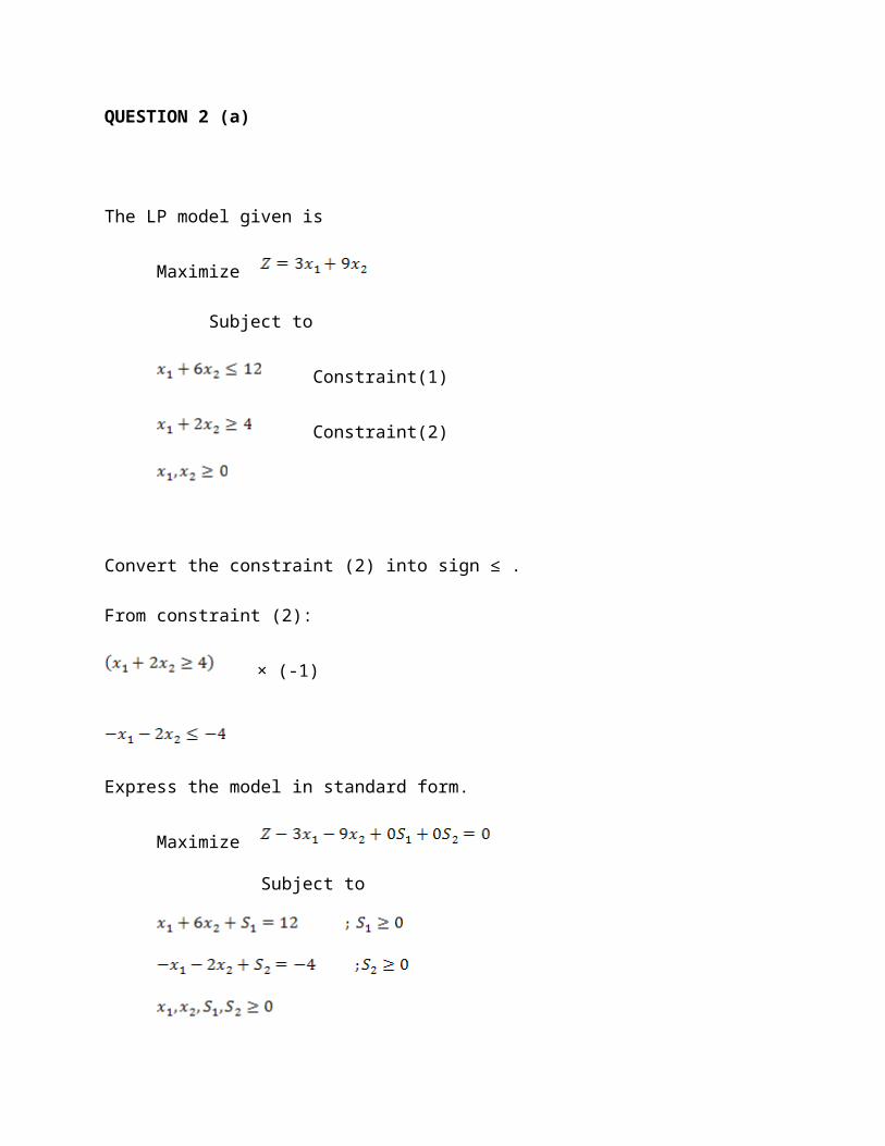
QUESTION 2 (a)

The LP model given is

Maximize

Subject to

Constraint(1)

Constraint(2)

Convert the constraint (2) into sign ≤ .

From constraint (2):

× (-1)

Express the model in standard form.

Maximize

Subject to

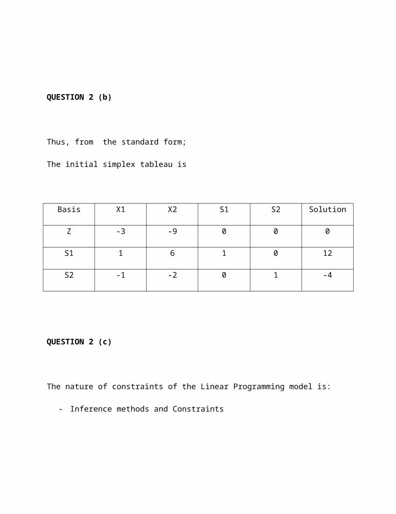
QUESTION 2 (b)

Thus, from the standard form;

The initial simplex tableau is

Basis X1 X2 S1 S2 Solution

Z -3 -9 0 0 0

S1 1 6 1 0 12

S2 -1 -2 0 1 -4

QUESTION 2 (c)

The nature of constraints of the Linear Programming model is:

- Inference methods and Constraints

QUESTION 3

a) Alternative optimal solutions – Model 2

Maximize

Subject to

(1)

(2)

(3)

(4)

Find all the points at which the lines intersects the and axes. Those constraints are can be

converted into equations or constraint lines.

From constraint (1):

When ; (0,3)

; (6,0)

From constraint (2):

When ; (0,8)

; (4,0)

From constraint (3):

When ; (0,1)

; (-1,0)

From constraint (4):

Sketch graphs :

Graphically, several combinations of the decision variables are optimal and we can select the most desirable optimal solutions. An optimal solution can be found at a corner or extreme point of the feasible region. Two and more optimal extreme points exist and all the points on the segment line connecting them are also optimal.

Thus, the model is alternative optimal solutions.

b) Unbounded solution – Model 4

Maximize

Subject to

(1)

(2)

Find all the points at which the lines intersects the and axes. Those constraints are can be

converted into equations or constraint lines.

From constraint (1):

From constraint (2):

When ; (0,0)

; (0,0)

Sketch graphs :

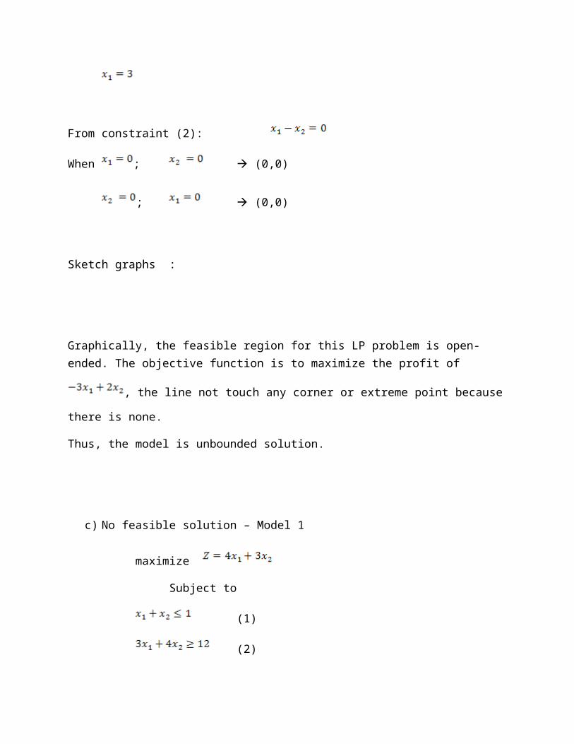
Graphically, the feasible region for this LP problem is open-ended. The objective function is to

maximize the profit of , the line not touch any corner or extreme point because there

is none.

Thus, the model is unbounded solution.

c) No feasible solution – Model 1

maximize

Subject to

(1)

(2)

Find all the points at which the lines intersects the and axes. Those constraints are can be

converted into equations or constraint lines.

From constraint (1):

When ; (0,1)

; (1,0)

From constraint (2):

When ; (0,3)

; (4,0)

Sketch graphs :

Graphically, it means that no feasible region exists; that is no point satisfies all the constraints and the non-negativity conditions simultaneously.

Thus, the model is no feasible solutions.

d) Redundant constraint – Model 3

Maximize

Subject to

(1)

(2)

(3)

Find all the points at which the lines intersects the and axes. Those constraints are can be

converted into equations or constraint lines.

From constraint (1):

When ; (0,8)

; (12,0)

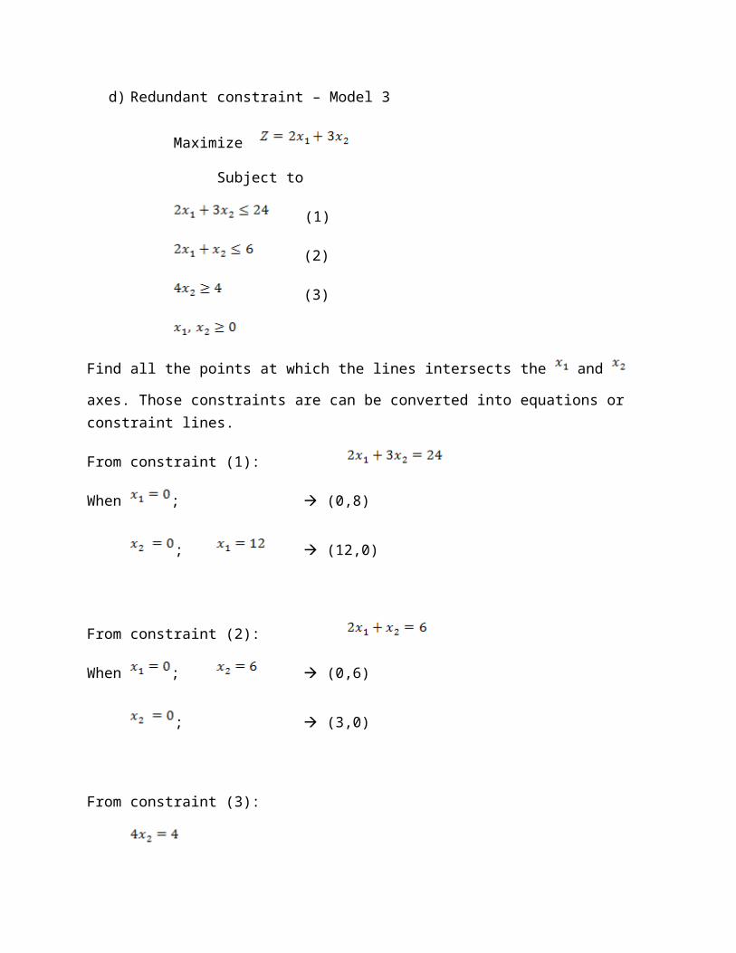
From constraint (2):

When ; (0,6)

; (3,0)

From constraint (3):

Sketch graphs :

Redundant constraint does not affect the feasible region and it can be removed from the problem.

Thus, the model is redundant constraints.

QUESTION 4 (a)

Given LP model is

Subject to

(1)

(2)

Find all the points at which the lines intersects the and axes. Those constraints are can be

converted into equations or constraint lines.

From constraint (1):

When ;

= 3.5 (0,3.5)

;

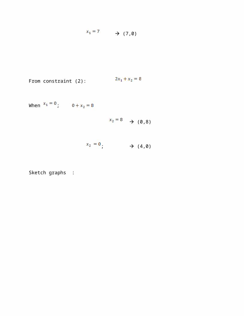
(7,0)

From constraint (2):

When ;

(0,8)

; (4,0)

Sketch graphs :

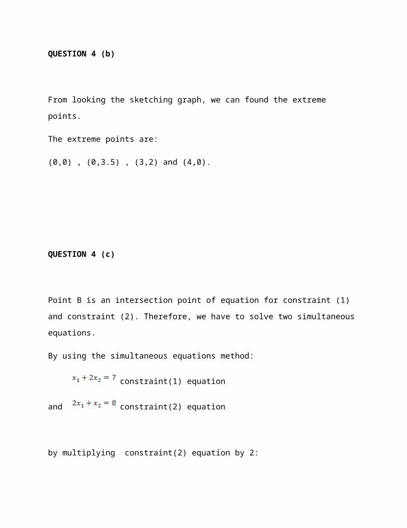
QUESTION 4 (b)

From looking the sketching graph, we can found the extreme points.

The extreme points are:

(0,0) , (0,3.5) , (3,2) and (4,0).

QUESTION 4 (c)

Point B is an intersection point of equation for constraint (1) and constraint (2). Therefore, we

have to solve two simultaneous equations.

By using the simultaneous equations method:

constraint(1) equation

and constraint(2) equation

by multiplying constraint(2) equation by 2:

Then, subtraction it to constraint (1) equation to obtain:

----------------------

Now, substitute the value of in constraint (2) equation to get the value of :

Thus, B has the coordinate (3,2) and we can compute the optimum value of the objective function to complete the analysis.

This gives

Thus,

The optimal solution occurs at (3,2) and its value is Z=13.

References

Dr Wan Rosmira Ismail(2010). SBMP4203 Linear Programming. Open University Malaysia.

Meteor Doc. Sdn. Bhd. Selangor Darul Ehsan.