scheduling mechanisms for efficient and safe automotive
TRANSCRIPT

DissertationTechnische Universität Braunschweig
Scheduling Mechanisms for Eicient and SafeAutomotive Systems Integration
Mahias Beckert


Scheduling Mechanisms for Eicient and Safe AutomotiveSystems Integration
Von der Fakultät für Elektrotechnik, Informationstechnik, Physikder Technischen Universität Carolo-Wilhelmina zu Braunschweig
zur Erlangung des Grades eines Doktors
der Ingenieurwissenschaen (Dr.-Ing.)
genehmigte Dissertation
von: Dipl.-Ing. Mahias Beckert
aus: Hildesheim
Eingereicht am: 30.04.2019
Mündliche Prüfung am: 25.10.2019
1. Referent: Prof. Dr.-Ing. Rolf Ernst2. Referent: Prof. Dr.-Ing. Stefan Kowalewski
Druckjahr: 2019

Dissertation an der Technischen Universität BraunschweigFakultät für Elektrotechnik, Informationstechnik, Physik
hps://doi.org/10.24355/dbbs.084-201911070747-5

Acknowledgements
The content of this dissertation was under development for almost seven years. Itis quite obvious that you never walk such a long way alone. During the past yearsseveral companions supported me on my way to completion of this dissertation.Without the support of Prof Dr. -Ing. Rolf Ernst nothing of this would havebeen possible, since he gave me the opportunity to take this final step in myacademical education.
The IDA is a well functioning institute and during my almost seven years asan employee I’ve learned very quickly how important the administrative partis. Without the help of Beina Boeger, Sabine Klöpper, Gudrun Leuer or PeterRüer one would most likely drown in the bureaucracy of german public service.Being a researcher is nothing without fellows which share the same demand-ing way. When I started at the IDA in mid 2012, I wasn’t even sure if I wouldmake it to the finish line. Especially in the first months or even years, findingthe right way of writing academic papers wasn’t easy for me. Without the helpof Moritz Neukirchner I’m not even sure if I would have kept on going. Underhis supervision I was able to publish my first academic paper, kick-starting my"academic journey". And speaking of journeys, publishing at international con-ferences definitely has its benefits. I will always remember my first trips to theUS with Philip Axer and Daniel Thiele. Same applies to the beer tasting withJohannes Schlatow in the crowded bars and streets of Seoul. The IDA in generalis a very valuable source of knowledge because of it’s very talented employees.
iii

The daily discussions during lunch or coee are something I miss, since I havele the institute. People like Holger Dinse or Mischa Möstl can provide you ananswer to life, the universe and everything. And in terms of discussions, sharinginterests in east european Sci-Fi literature with my long term oice mate AdamKostrzewa made even the most boring day interesting. During my time at theinstitute I supervised several students and one of them was more persistent thanthe others. Kai Gemlau started to work for me in the beginnings of his bachelorstudies and later joined the institute as an employee aer his master thesis. Itwas a pleasure to watch his development over the years, and I am grateful for theinput and feedback he gave me for my work. Generally speaking, I am gratefulto all my colleagues at IDA that I was able to spend so much time with such nicepeople. I don’t regret a single minute of it.
One of the most common tasks a researcher has to deal with is, to createreviews for conference submissions. Well, what can I say? I can imagine morebeautiful tasks. Creating reviews is a very time-consuming process and takesa lot of eort, especially if you’re not familiar with the author’s other works.Because of this, I am grateful that Prof. Dr. -Ing. Stefan Kowalewski investedthe time to review this dissertation. One thing I oen missed in the submissionsI got for review were real-world test-cases from the industry. Sometimes thiswasn’t needed for the conference, but more oen there were hardly any test-cases available at all. At this point I am happy that I had the opportunity to workwith people like Hermann von Hasseln or Tobias Sehnke who both provided mea deep view into the design of existing automotive systems.
At the end of the day you go home aer work, sometimes in good mood,sometimes in a bad mood. But always with the knowledge that your friendsand family support what you are doing. I am grateful, that my parents Elisabethand Frank, as well as my sisters Julia and Stefanie have always supported mein what have I done. I thank my friends Florian and Johannes for our regularboardgame and brewing sessions, which always provide the perfect counterpartto a stressful week. Same applies to the “Doko guys” Andy, Jonas, Carsten andChristoph for the shared time during our legendary weekend excursions. Butmost of all, I would like to express my deepest respect to my wonderful fiancéeJanina. Together with our son Mika she always had my back and motivated meto finish my work. Thank you for supporting and enduring me the past sevenyears, even in my worst days.
iv
Kurzfassung
Auf Grund moderner Themen wie dem assistierten Fahren steigt der Bedarf anRechenleistung in aktuellen Fahrzeugen seit einigen Jahren kontinuierlich an.Um die erforderliche Rechenleistung zur Verfügung zu stellen, konzentriertensich die Prozessorhersteller in der Vergangenheit auf den Wechsel von Einzel-zu Mehrkern-CPU Architekturen. Durch die zusätzliche Leistung ermöglichensolche Mehrkern-CPUs die Integration von zuvor einzeln ausgeführten Soware-komponenten auf derselben Hardware, was zu einer Reduktion der Gesamtzahlan ECUs in Fahrzeugen beiträgt. Während Mehrkern-CPUs in Standard Com-putersystemen bereits seit langem Verwendung finden, ist der eiziente Einsatzin eingebeeten Systemen mit Echtzeitanforderungen häufig schwierig. Für dieIntegration von mehreren Sowarekomponenten auf derselben Hardware mussdie Störungsfreiheit zwischen den einzelnen Komponenten für eine sichere Aus-führung gewährleistet sein. Ein weiteres Problem besteht häufig bei bereits ex-istierender Legacy-Soware, welche für die Ausführung auf einer einzelnen CPUwährend der Entwicklung optimiert wurde und daher nicht ohne weiteres aufmehrere Prozessorkerne verteilt werden kann.
Diese Dissertation beschreibt zwei Mechanismen, welche eine sinnvolle Nut-zung der zusätzlichen Rechenleistung ermöglichen sollen. Der erste Mechanis-mus verwendet partitionsbasierter Virtualisierung, welche in der Avionik bereitsin der Vergangenheit in Form von ARINC653 Verwendung gefunden hat. Zielist hierbei, mehrere Sowarekomponenten auf derselben ECU zu integrieren.
v

Die Störungsfreiheit wird durch die Ausführung über einen Hypervisor erreicht,welcher die partitionsbasierte Virtualisierung implementiert und überwacht.
Zweitens wird die Integration des LET Paradigmas in eine automobile Sys-temarchitektur gezeigt, welches eine blockierungsfeie Synchronisation der Kom-munikation über Kerngrenzen hinweg ermöglicht. Generell erlaubt dieser Mech-anismus eine Synchronisation von Soware über mehrere Prozessorkerne hin-weg, was sowohl für die parallele Ausführung von Legacy-Soware als auch vonvirtualisierten Partitionen genutzt werden kann.
Der wissenschaliche Beitrag dieser Dissertation ist in erster Linie die In-tegration beider Mechanismen in einen automobilen Kontext. Dazu gehöreneine Analyse der Antwortzeiten sowie eine Diskussion über bestimmte Heraus-forderungen bei der Implementierung. Beide Mechanismen werden in einer Pro-totyp Implementierung evaluiert und die Ergebnisse präsentiert.
vi

Abstract
During the last years, the demand of computing power in modern cars has risencontinuously, especially due to modern topics like assisted driving. In order toprovide the required computing power, the chip manufactures focused in the paston the switch from single- to multicore CPU architectures. Such powerful mul-ticore CPUs allow the integration of multiple soware components on the samehardware, therefore reducing the overall number of ECUs inside a car. Whilemulticore CPUs are well-known in general purpose computing, the eicient usein highly embedded systems with real-time requirements is more challenging.For the integration of multiple soware components on the same hardware, free-dom interference between those components must be enforced to ensure a safeexecution. In case of existing legacy soware the problem is oen based on pre-viously optimized execution for a singlecore CPU and as a result the parallelexecution of such legacy soware on multiple cores is not straight forward.
This dissertation describes two possible scheduling techniques in order to en-able sensible use of the new available computing power. The first mechanismuses partition based virtualization, which has been a well-known technique inavionics with ARINC653. Objective is the integration of multiple soware com-ponents on the same ECU. Freedom from interference is achieved through theexecution on top of a hypervisor, implementing and monitoring the partitionbased virtualization. Second, an integration of the LET paradigm into an auto-motive system architecture, enabling a lock-less synchronized communication
vii

across core boundaries. In general, such a mechanism allows a synchronizationof soware among multiple CPU cores. This allows synchronization across coreboundaries which can be used for both, existing legacy soware as well as virtu-alized partitions.
The scientific contribution of this dissertation is primarily the integration ofboth mechanisms into an automotive context. This includes a response timeanalysis as well as a discussion of certain implementation challenges. Both mech-anisms will be evaluated in a prototype implementation, including a discussionof the results.
viii

Contents
1 Introduction 11.1 Contribution . . . . . . . . . . . . . . . . . . . . . . . . . . . . . . . 71.2 Outline . . . . . . . . . . . . . . . . . . . . . . . . . . . . . . . . . . 8
2 Trends in Automotive ECU Architectures 92.1 Hardware Architecture . . . . . . . . . . . . . . . . . . . . . . . . . 9
2.1.1 AURIX . . . . . . . . . . . . . . . . . . . . . . . . . . . . . . . 102.1.2 R-Car H3 . . . . . . . . . . . . . . . . . . . . . . . . . . . . . . 142.1.3 Comparison . . . . . . . . . . . . . . . . . . . . . . . . . . . . 17
2.2 Soware Architecture . . . . . . . . . . . . . . . . . . . . . . . . . . 182.2.1 Application . . . . . . . . . . . . . . . . . . . . . . . . . . . . 202.2.2 Operating System . . . . . . . . . . . . . . . . . . . . . . . . . 242.2.3 Soware Stacks . . . . . . . . . . . . . . . . . . . . . . . . . . 282.2.4 Adaptive AUTOSAR . . . . . . . . . . . . . . . . . . . . . . . . 30
2.3 Problem Statement . . . . . . . . . . . . . . . . . . . . . . . . . . . 322.3.1 Eicient Hypervisor Scheduling . . . . . . . . . . . . . . . . . 322.3.2 Multicore Synchronization . . . . . . . . . . . . . . . . . . . . 34
3 System Model 393.1 Execution Model . . . . . . . . . . . . . . . . . . . . . . . . . . . . . 403.2 Response Time Analysis . . . . . . . . . . . . . . . . . . . . . . . . . 45
ix

CONTENTS
4 ARINC653 based Hypervisor Scheduling 494.1 System model addition for hierarchical scheduling . . . . . . . . . . 494.2 IRQ handling in virtualization environments . . . . . . . . . . . . . 524.3 Monitoring based IRQ shaping in partitioned virtualization envi-
ronments . . . . . . . . . . . . . . . . . . . . . . . . . . . . . . . . . 544.4 WCRT analysis . . . . . . . . . . . . . . . . . . . . . . . . . . . . . . 594.5 Time Cycle Optimization . . . . . . . . . . . . . . . . . . . . . . . . 62
4.5.1 Optimization algorithm . . . . . . . . . . . . . . . . . . . . . . 624.5.2 Laxity based time cycle bound . . . . . . . . . . . . . . . . . . 654.5.3 Slack distribution . . . . . . . . . . . . . . . . . . . . . . . . . 67
4.6 Formal limitations of IRQ shaping . . . . . . . . . . . . . . . . . . . 69
5 Sporadic Server based Budget Scheduling 715.1 Isolation bound . . . . . . . . . . . . . . . . . . . . . . . . . . . . . 73
5.1.1 Scheduler setup . . . . . . . . . . . . . . . . . . . . . . . . . . 745.1.2 Service provisioning . . . . . . . . . . . . . . . . . . . . . . . . 765.1.3 Work conserving scheduling . . . . . . . . . . . . . . . . . . . 78
5.2 WCRT Analysis . . . . . . . . . . . . . . . . . . . . . . . . . . . . . 795.2.1 Without background scheduling . . . . . . . . . . . . . . . . . 805.2.2 With background scheduling . . . . . . . . . . . . . . . . . . . 815.2.3 Simplified for queue-based background scheduling . . . . . . 87
5.3 Comparison and expectations . . . . . . . . . . . . . . . . . . . . . 88
6 The LET Paradigm as Coordination Instance 916.1 The LET Paradigm . . . . . . . . . . . . . . . . . . . . . . . . . . . . 936.2 Lock-less Zero-Time Communication . . . . . . . . . . . . . . . . . 966.3 LET in Automotive Soware . . . . . . . . . . . . . . . . . . . . . . 101
7 Implementation Challenges 1077.1 SPS based Budget Scheduling . . . . . . . . . . . . . . . . . . . . . 110
7.1.1 Timer usage . . . . . . . . . . . . . . . . . . . . . . . . . . . . 1117.1.2 SPS CBAPI . . . . . . . . . . . . . . . . . . . . . . . . . . . . . 1137.1.3 Scheduler implementation . . . . . . . . . . . . . . . . . . . . 117
7.2 LET implementation with Zero-Time Communication . . . . . . . . 1227.2.1 Hardware Port . . . . . . . . . . . . . . . . . . . . . . . . . . . 1257.2.2 OS Port . . . . . . . . . . . . . . . . . . . . . . . . . . . . . . . 1267.2.3 Memory usage . . . . . . . . . . . . . . . . . . . . . . . . . . . 129
8 Evaluation 1338.1 SPS based budget scheduling . . . . . . . . . . . . . . . . . . . . . . 134
8.1.1 WCRT Analysis . . . . . . . . . . . . . . . . . . . . . . . . . . 134
x

CONTENTS
8.1.2 Response time measurements . . . . . . . . . . . . . . . . . . 1408.1.3 Runtime and memory overhead . . . . . . . . . . . . . . . . . 147
8.2 LET implementation with Zero-Time Communication . . . . . . . . 1488.2.1 Runtime and memory overhead . . . . . . . . . . . . . . . . . 1488.2.2 Overload behavior . . . . . . . . . . . . . . . . . . . . . . . . . 156
9 Conclusion 159
A Publications 163A.1 Reviewed . . . . . . . . . . . . . . . . . . . . . . . . . . . . . . . . . 163A.2 Unreviewed . . . . . . . . . . . . . . . . . . . . . . . . . . . . . . . . 165
List of Figures 167
List of Tables 169
List of Code 171
Acronyms 173
Bibliography 179
xi

CONTENTS
xii

CHAPTER1
Introduction
“DON’T PANIC!”
- The Hitchhiker’s Guide to the Galaxy
The role of soware and electronic hardware is becoming increasingly importantin modern vehicles. Over the years the so called Electric/Electronic Architec-ture (EEA) of cars has evolved continuously. While the EEA itself is of no interestto the driver of a car, the functionality it implements defines the driving expe-rience. The EEA consists of a set of Electronic Control Units (ECUs) which areconnected via a set of buses and/or networks. Each ECU houses soware whicheither provides some specific functionality or is part of a bigger function whichis distributed on several ECUs.
Current and presumably future ECUs are developed based on the InternationalStandard 26262: “Road vehicles - Functional safety” (ISO26262) [66], which rep-resents the standard for functional safety of road vehicles. The ISO26262 was de-veloped based on the generic International Electrotechnical Commission, Stan-dard 61508: “Functional Safety of Electrical/Electronic/Programmable ElectronicSafety-related Systems” (IEC61508) [65] taking into account the requirementsand needs of the automotive industry. Comparable standards to the ISO26262are also available in other domains. As an example, in avionics the DO-178B, So-ware Considerations in Airborne Systems and Equipment Certification (DO-178B)[94] and its counterpart DO-254, Design Assurance Guidance for Airborne Elec-tronic Hardware (DO-254) [95] define functional safety for soware and hard-
1

CHAPTER 1. INTRODUCTION
ASILA B C D
SPFM - > 90% > 97% > 99%LFM - > 60% > 80% > 90%PMHF - < 10−7h−1 < 10−7h−1 < 10−8h−1
FIT - < 100 < 100 < 10
Table 1.1: ASIL hardware fault metric specification
ware components in airborne systems. ISO26262 defines functional safety as “ab-sence of unreasonable risk due to hazards caused by malfunctioning behaviourof E/E systems” [66].
One of the major definitions of the ISO26262 are Automotive Safety IntegrityLevels (ASIL), which are the counterpart to the Safety Integrity Levels (SIL) fromIEC61508. The ASIL classification is used to define automotive-specific hardwarerequirements in order to preserve functional safety. There are four integrity lev-els available, starting with low safety requirements in ASIL A up to the moststringent safety requirements in ASIL D. In general, ISO26262 doesn’t assume asystem to be perfect without any kind of hardware or soware faults. Instead,the incidence of allowed faults is limited. Table 1.1 gives a fault metric overviewof the dierent integrity levels based on random hardware failures.
The first entry in Table 1.1 denotes the Single-Point Fault Metric (SPFM).SPFM indicates the robustness against untrapped hardware faults that wouldcause an immediate violation of functional safety. The second entry denotesthe Latent Fault Metric (LFM). Again, LFM indicates the robustness against un-trapped hardware faults. But instead of immediate, latent violations are takeninto account. As an example for ASIL C, a maximum of 3% of all untrappedsingle-point and 20% of all untrapped latent faults are allowed to cause viola-tions of functional safety. Next the Probabilistic Metric for random HardwareFailures (PMHF) describes the overall number of allowed untrapped hardwarefailures per hour. For a beer representation this can be converted into Faults InTime (FIT), which denotes the number of allowed failures per one billion hours.
Another important requirement from ISO26262 is the so called freedom frominterference defined as “absence of cascading failures between two or more ele-ments that could lead to the violation of a safety requirement” [66]. In case ofsoware components this means, that a failure in component A will never causea failure in component B and vice versa. Although the ISO26262 does not defineany specific mechanisms to it, it makes sense to take a look at possible sourcesof danger with regard to freedom from interference. In general there are threedierent sub-areas that need to be considered.
2

Temporal Isolation: The temporal behavior of component A is independentof component B, even if component B crashes while blocking the CentralProcessing Unit (CPU) or actively tries to disturb component A. Usually anoperating system ensures temporal isolation.
Spatial Isolation: A memory access of component B can never overwrite pri-vate data of component A, unless otherwise specified. This must be also thecase, even if component B access the memory accidentally through a wildpointer. Usually spatial isolation is ensured by the CPU in hardware witha Memory Protection Unit (MPU) or Memory Management Unit (MMU).
Deadlock prevention: The access to shared resources or peripherals is usuallycoordinated with mechanisms like semaphors. In order to provide dead-lock prevention, it must be ensured that a crashed component cannot blocka shared resource permanently. A known technique for deadlock preven-tion is the use of watchdogs [15].
All of these sub-areas rely on a combination of hardware and soware mech-anisms. While classical temporal isolation usually requires only a timer witha suicient resolution as time-base, the corresponding soware executed dur-ing runtime is oen much more complex. On the other hand, spatial isolationis primarily ensured in hardware. The corresponding soware is oen limitedto an accurate configuration of MPU or MMU during startup. For watchdogsdierent implementations from tick based soware implementations to distincthardware modules are possible. In general, achieving freedom from interferencealways requires a combination of special hardware and soware mechanisms.
As the number of functions in a car increases, also the load on each ECU andinterconnect rise. To implement further more functionality in a car, the usedhardware inside an ECU must be replaced in order to gain processing power.Since a few years, the evolution of processors in embedded systems has gone thesame way as in consumer electronics. The processors clock speed as well as thenumber of integrated cores has increased. As a result, ensuring freedom frominterference gets more and more important, since otherwise single faults mayhave an even bigger impact to the system. Nevertheless, faster processors do notreduce the loads on the interconnects. The migration from single to multicoreCPUs is also challenging. Oen existing legacy soware developed for singlecoreCPUs is reused, which might lead to problems in case of coordination and dataconsistency.
With respect to temporal and spatial isolation, integrating further more func-tions on a single ECU gets even more sophisticated. As already mentioned,spatial isolation is usually achieved through the use of hardware functional-ity like memory protection or management. When implementing spatial iso-
3

CHAPTER 1. INTRODUCTION
lation this way, it is required to reconfigure the corresponding hardware mod-ule (MPU/MMU) each time a dierent soware component is executed. In theworst-case this means that the hardware must be reconfigured on each switchbetween the dierent soware components, which can introduce major runtimeoverhead.
A counter measure to this additional overhead can directly be derived fromthe fact that most of the executed code is existing legacy soware. Usually, ex-isting legacy soware has been executed flawlessly before on a single ECU, oenwithout any kind of hardware based memory protection. Instead, freedom frominterference has been ensured through extensive testing and verification. With ahigher number of soware components on a single ECU, the costs and expensesfor testing and verification rise. A possible method to mitigate this could be par-titioning. General idea is to bundle multiple soware components into largerpartitions. The verification is then performed separately on each single parti-tion, with a much smaller number of soware components inside. Ideally thisverification has been already performed before for an older ECU but the samecombination of soware components. The handling of dierent partitions is thenperformed by a soware which provides freedom from interference between par-titions. A possible way to provide temporal as well as spatial isolation betweendierent partitions is to use an embedded hypervisor for virtualization.
Virtualization is a well-known approach in the field of general purpose com-puting. Oen one physical machine hosts 20 virtual ones or even more. Sincehardware in the embedded domain gets more and more powerful, techniqueslike virtualization gain aention. Especially in domains which are not as costdriven as the automotive sector, virtualization with more powerful CPUs was al-ready considered some time ago. With the Integrated Modular Avionics (IMA)architecture and Aeronautical Radio Incorporated Avionics Application StandardSoware Interface (ARINC653) [93] as a corresponding implementation descrip-tion, virtualization techniques have become part of a standardized soware ar-chitecture in safety-critical systems. This was possible, as in avionics the costsper unit aren’t as important as in the automotive industry due to much highersystem costs compared to the electronic and soware parts. However, combin-ing multiple computation units on a single hardware reduces the overall weight,which is much more important for an airplane.
Figure 1.1 shows the basic setup of two virtualized applications according toARINC653. Each application is encapsulated in a partition, executed with min-imized privileges in the user mode of the CPU. In addition to an application,each partition might also contain an Partition Operating System (OS) (POS). Theprivileged system mode of the CPU is reserved for the hypervisor which providesaccess to the underlying hardware. With the Application Executive (APEX) [107]Application Programming Interface (API), an ARINC653 conformant hypervisor
4

Interconnect
Sys
tem
Mo
de
Use
r M
od
e Partition 1
Hypervisor
Partition 2
Hardware Platform
APEX API
Hardware Driver
Partition OS Partition OS
Application Application
Figure 1.1: Simplified hypervisor based system setup
provides a set of functions to access hypervisor functionality from a partition[93].Commercial hypervisor implementations like PikeOS [70] or VxWorks 653 [116]usually provide an own POS or API implementation in addition to the APEXAPI. As an example, both mentioned implementations provide also a PortableOS Interface (POSIX) for virtualized applications. Also, PikeOS has already beenconsidered as a possible hypervisor for the automotive domain [29], despite itsorigins in avionics.
As shown in Figure 1.1 applications are isolated from each other. The hyper-visor is responsible at that point to ensure spatial and temporal isolation. Asmentioned before, spatial isolation is usually achieved based on either an MPUor MMU. A side eect of the use of memory protection or management for spa-tial isolation is, that not only a safe but also secure execution of soware insidea partition is achieved. Resulting from this, the use of MPU or MMU enables asecure execution of possible intellectual property of dierent soware supplierson the same ECU. With the hypervisor occupying the CPU’s system mode, ithas full control of either MPU or MMU. To provide spatial isolation, the hyper-visor simply reconfigures the corresponding register when switching executionbetween dierent partitions based on a static configuration.
While spatial isolation is primarily based on core features of a modern CPU,temporal isolation instead depends primarily on the implemented scheduling al-gorithm. Oen only an accurate timebase is needed to implement a schedulingstrategy. Nowadays, even in the smallest Microcontroller (µC) such a timebasecan be realized with a timer module. A simple way to describe temporal iso-lation is, that the time a soware component needs to finish its computation,is independent of the behavior of all other soware components on the same
5

CHAPTER 1. INTRODUCTION
ECU. We provide a more versatile and formal description of temporal isolationin Section 4.1.
ARINC653 achieves temporal isolation through a simple Time Division Mul-tiple Access (TDMA) scheduling on partition-level. In general, the dierent par-titions get executed in a static order for fixed amount of time. An obvious draw-back of such a static execution is the handling of sporadic events like InterruptRequests (IRQs). As a simple example based on Figure 1.1, if the ECU is execut-ing partition 1, IRQs for partition 2 can not be processed during that time. Thisis even the case if partition 1 has no work to do. Chapter 4 explains this issue inmuch more detail. In case of avionics, this isn’t as bad as expected. First of allthe entire IMA is a uniform architecture with interconnects like ARINC429/629 orAvionics Full DupleX Switched Ethernet (AFDX) between dierent ECUs, whichmatch the partition-level TDMA scheduling. Second, usually avionics aren’t thattiming sensitive and as a result, sensors or actors might be processed based onpolling and not on IRQs due to beer predictability. And third, if a sensor or actorneeds a close interaction to an µC in order to work properly, it is encapsulatedwith an own µC and connected to the already mentioned interconnect, whichagain matches the partition-level TDMA scheduling.
Adding additional hardware is possible due to the less cost sensitivity in avion-ics. This is dierent for the automotive domain, which has a much higher volumeand costumers which are usually not willing to spend a lot of money. As a result,the automotive industry tries to avoid unnecessary ECUs at that point and oenconnects sensors or actors directly. Also, IRQs are much more timing critical inthe automotive domain. As an example, if a crash of a car is registered, safetymechanisms like seatbelt tensioner or airbags must be activated within a fewmilliseconds. But not only in a worst-case scenario like a crash, also in normaldriving situations a fast processing of IRQs is absolutely necessary. Let’s assumethe driver wants to accelerate the car and pushes the pedal to the metal. Thebehavior of the car expected by the driver is to accelerate within a fraction ofa second. What the driver doesn’t know is, that such a simple command mightinvolve several ECUs inside a car for input processing, torque coordination andengine control. And inside all of those ECUs the processing must be fast in or-der to enable the expected response behavior of the car. Without a fast IRQsprocessing, such a behavior is hard to achieve.
Beside the need of a fast IRQ processing, there is also another problem. Theparallel execution of soware on multicore CPUs isn’t addressed by ARINC653,since the definition only include singlecore CPUs. In order to deploy an auto-motive application on a multicore platform, it is necessary to know the dataflowbetween dierent soware components. The best case would result in a system,where the soware on dierent cores is completely independent of each other.Practically this is oen out of reach and dependencies exists between the tasks
6

1.1. CONTRIBUTION
on dierent cores. Thus, core-to-core communication should be minimized basedon an extensive dataflow analysis of the system soware, but assuming that itcan be eliminated completely is way too optimistic.
A possible method, how dependencies can be identified in automotive legacysoware, has been introduced in [59]. The proposed algorithm groups indepen-dent soware parts, which can run in parallel without additional synchroniza-tion. Dependent soware parts are then sequenced aer each other. For eachdependency across multiple cores a synchronization method or special commu-nication mechanism is needed. Oen hardware architectures in the automotiveindustry do not support special core-to-core communication mechanisms. Forminimal overhead, lock-free communication based on shared memory variablesis oen used. Such a lock-free communication can be implemented in two dif-ferent ways. The simple solution is a “don’t care” behavior for input variables. Inthis case it does not maer if a read-aer-write behavior is enforced or not. Butsuch an approach only works for specific algorithms. A possible solution to this isthe Logical Execution Time (LET) paradigm, which defines global points in timewhen data is wrien or read. This way, only a global time is needed to synchro-nize the soware on dierent cores. Even though the LET paradigm is alreadyconsidered to be part of the Automotive Open System Architecture (AUTOSAR)in the future, an open question is still the versatility of LET and the way how itcan be integrated into the existing architecture.
1.1 Contribution
In general, utilizing the newly available computing power is challenging in dier-ent ways. On the one hand, sharing a powerful ECU with multiple applicationsmay violate freedom from interference. On the other hand, distributing a pre-vious singlecore applications to multiple cores may not be that easy either. Thecontribution of this work is therefore structured in two main topics.
First, we propose a system architecture which provides virtualization mecha-nisms with real-time capabilities. The proposed system architecture is based onthe ARINC653 standard, which relies on a static time partitioning. In order toachieve a beer IRQ performance we provide dierent modifications to the origi-nal architecture. This includes a monitoring based IRQ shaping, an optimizationalgorithm for time partitions and a Sporadic Server (SPS) based budget schedul-ing on partition-level. As a formal proof, we cover all proposed mechanisms withan Response Time Analysis (RTA) based on Compositional Performance Analy-sis (CPA) implementing the well-known multiple event busy-window [77, 104].The paper published in context with this work are [28, 23, 26, 24].
Second we take a look the LET paradigm as a possible coordination instance
7

CHAPTER 1. INTRODUCTION
in order to execute existing automotive soware on multicore processors. Theapplicability of the LET paradigm is discussed and an integration method is pro-posed. This includes additional methods for an RTA as well as an upper inter-ference bound. The work on this topic is primary based on [27], [25] and a talkgiven at [44].
For both topics we intensively discuss the implementation challenges, withfocus on eiciency on existing hardware. As a result of the discussion we intro-duce working implementations for both topics, which are then used to evaluatethe proposed mechanisms.
1.2 Outline
The remainder of this dissertation thesis is structured as followed. Chapter 2gives an overview of the current architecture of modern ECUs. This includes thehardware as well as the soware architecture. At the end of this chapter, wefinalize the problem statement based on existing hardware and soware archi-tecture in the automotive domain. Chapter 3 introduces the system model. Forthis purpose, the general RTA framework and used notation is explained.
Chapter 4 provides an overview of the scheduling technique described byARINC653. Also, possible problems regarding IRQ handling are explained, as wellas a possible solution is introduced. In order to generate valid system configura-tions, we also provide a partition size optimization based on a RTA for ARINC653based system. Chapter 5 shows how to map the system explained in Chapter 4to an SPS based partition scheduling. In order to provide the same degree of suf-ficient temporal independence as for ARINC653, we introduce a budget basedpartition scheduling in combination with the SPS mechanism. The budget basedscheduling is then extended to a fully work conserving scheduler. All providedmechanisms in this chapter are again covered with an RTA. Chapter 6 gives anintroduction to the LET paradigm and shows how this can be applied to an auto-motive soware architecture. This includes the discussion of a task distributionstrategies and possible integration mechanisms.
Chapter 7 discusses the implementation challenges of the mechanisms de-scribed in Chapter 4, 5 and 6. Here we focus on specific aspects relevant forautomotive systems. This includes primarily the described hardware/sowarearchitecture from Chapter 2 as well as general programming techniques for codewith improved temporal predictability. Chapter 8 evaluates the proposed mech-anisms. This includes the actual implementations as well as the provided RTA.Chapter 9 summarizes the outcome of the dissertation and outlines possible fu-ture work.
8

CHAPTER2
Trends in Automotive ECU Architectures
“Soware is like sex: It’s beer when it’s free”
- Linus Torvalds
Main task of this chapter is to convey some basic knowledge about the architec-ture of current and future ECUs, in order to understand the later finalized prob-lem statement and proposed solutions. The chapter starts with an inside into thehardware and soware architecture of modern ECUs. This includes two multi-core architectures which can be considered as examples for dierent automotiveuse-cases. On the soware side, an insight into the structure of automotive ap-plications and the surrounding Runtime Environment (RTE) is given. Based onboth, the underlying hardware and the existing soware framework, the alreadystarted problem statement from Chapter 1 is finalized.
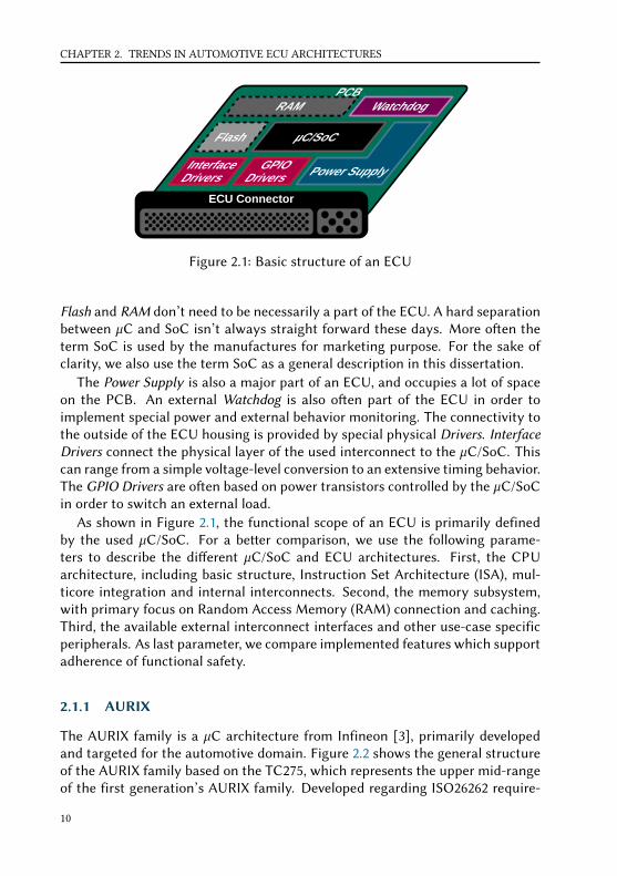
2.1 Hardware Architecture
Figure 2.1 gives a short overview of the essential hardware elements of a modernECU. The mechanical structure of an ECU is based on a Printed Circuit Board(PCB) inside a standardized housing with an ECU-specific connector. Usually themost important part of an ECU is the central µC or in some cases an System Ona Chip (SoC). Both, µC and SoC describe systems including one or more CPUs,integrated peripherals and memory controllers. A µC usually directly includesFlash and RAM, while those are oen separate for some SoCs. Therefore, external
9
CHAPTER 2. TRENDS IN AUTOMOTIVE ECU ARCHITECTURES
ECU Connector
Figure 2.1: Basic structure of an ECU
Flash and RAM don’t need to be necessarily a part of the ECU. A hard separationbetween µC and SoC isn’t always straight forward these days. More oen theterm SoC is used by the manufactures for marketing purpose. For the sake ofclarity, we also use the term SoC as a general description in this dissertation.
The Power Supply is also a major part of an ECU, and occupies a lot of spaceon the PCB. An external Watchdog is also oen part of the ECU in order toimplement special power and external behavior monitoring. The connectivity tothe outside of the ECU housing is provided by special physical Drivers. InterfaceDrivers connect the physical layer of the used interconnect to the µC/SoC. Thiscan range from a simple voltage-level conversion to an extensive timing behavior.The GPIO Drivers are oen based on power transistors controlled by the µC/SoCin order to switch an external load.
As shown in Figure 2.1, the functional scope of an ECU is primarily definedby the used µC/SoC. For a beer comparison, we use the following parame-ters to describe the dierent µC/SoC and ECU architectures. First, the CPUarchitecture, including basic structure, Instruction Set Architecture (ISA), mul-ticore integration and internal interconnects. Second, the memory subsystem,with primary focus on Random Access Memory (RAM) connection and caching.Third, the available external interconnect interfaces and other use-case specificperipherals. As last parameter, we compare implemented features which supportadherence of functional safety.
2.1.1 AURIX
The AURIX family is a µC architecture from Infineon [3], primarily developedand targeted for the automotive domain. Figure 2.2 shows the general structureof the AURIX family based on the TC275, which represents the upper mid-rangeof the first generation’s AURIX family. Developed regarding ISO26262 require-
10

2.1. HARDWARE ARCHITECTURE
Figure 2.2: AURIX 1 generation µC architecture [4]
ments the AURIX family allows certification of up to ASIL-D [3]. Although firstdetails about the second generation AURIX are already available [3], we primar-ily focus on the details of the first generation as those are available to the public.Therefore, all data mentioned refer to the first generation AURIX family unlessotherwise stated.
CPU architecture and SoC structure
The AURIX family is a 32-bit Reduced Instruction Set Computer (RISC) archi-tecture, implementing multiple TriCore [5] CPUs on the same chip. There aredierent hardware series available, implementing either two or three TriCoreCPUs for the first and up to six CPUs for the second generation AURIX SoCs.The maximum clock frequency of the integrated TriCore CPUs is 300 MHz anddepends on the actual series.
The example from Figure 2.2 shows a setup with three TriCore v1.6 CPUs.Each TriCore consists of a general purpose CPU, a Floating Point Unit (FPU)
11

CHAPTER 2. TRENDS IN AUTOMOTIVE ECU ARCHITECTURES
and a Digital Signal Processor (DSP). For the shown TC275, two dierent vari-ants of the TriCore CPU are used. An energy optimized v1.6e and a performanceoptimized v1.6p. The dierence between both versions is primarily the pipelinestructure. The actual combination of TriCore CPUs depend on the AURIX vari-ant. As an example, the TC295 implements three v1.6p CPUs compared to theTC275 with one v1.6e and two v1.6p. The dierent TriCore CPUs are connectedamong each other with a System Resource Interconnect (SRI) cross bar, whichalso connects the CPU-external memory subsystem and a Direct Memory Ac-cess (DMA) controller. Additional periphery is available through the system pe-ripheral bus.
Memory Subsystem
The memory subsystem can be divided into CPU-internal and external memory.As the actual sizes for both types dier for various AURIX variants, we state themaximum sizes. It is also important that the first generation AURIX µCs do notprovide any interface for o-chip memory.
As mentioned before, the CPU-external memory is connected via the SRI. Itconsists of a Program Memory Unit (PMU) and a Local Memory Unit (LMU). ThePMU provides program flash memory and a data flash memory for non-volatilevariables. Overall size of the PMU ranges up to 8 MB program and 768 kB dataflash. The LMU provides a global Static Random-Access Memory (SRAM) with32 kB memory.
Beside PMU and LMU, each TriCore CPU also contains an internal SRAM andadditional caches. The CPU-internal SRAM is divided into Program Scratch-PadSRAM (PSPR) and Data Scratch-Pad SRAM (DSPR). Both, PSPR and DSPR aretightly coupled to the corresponding TriCore CPU and provide a fast memoryaccess. As all memories share the same address space, remote access to PSPRor DSPR of another TriCore CPU through the SRI is also possible. The maxi-mum SRAM sizes for PSPR/DSPR are 32 kB / 240 kB per TriCore CPU. EachTriCore CPU also provides its own data and instruction cache, implemented asSRAMs. While an access to the CPU-internal SRAM does not achieve any speedup through the cache, it is noticeable for remote accesses through the SRI. Im-portant is at this point, that there is no coherency protocol implemented in thecaches. As a result global data, shared across multiple TriCore CPUs, should notbe cached. Otherwise, inconsistent data might be the outcome. The maximumcache sizes for data/instruction cache are 8 kB / 32 kB. As the caches are imple-mented as SRAMs, they can be deactivated and used as an extension to PSPRand/or DSPR.
12

2.1. HARDWARE ARCHITECTURE
Interconnects and peripherals
The AURIX family provides a wide range of interconnects from the automotiveindustry. The Local Interconnect Network (LIN) provides the lowest bandwidthand is represented as ASCLIN module in Figure 2.2. In case of the top of therange implementation the AURIX provides four LIN interfaces. Next there isthe MultiCAN+ module, implementing both Controller Area Network (CAN) andCAN with Flexible Data-Rate (CAN-FD) interfaces. The maximum accumulatednumber of either CAN or CAN-FD is limited to six interfaces implemented bytwo MultiCAN+ modules. In the case of higher bandwidth, likely used as a back-bone interconnect of dierent domain, the AURIX supports two FlexRay inter-faces. For even more bandwidth, the AURIX also provides one 100 MBit/s Ether-net Media Access Controller (MAC).
The number of available interconnects directly defines one use-case for theAURIX family. This use-case is the integration as central gateway or centralcontroller ECU with connection to several car domains [64]. Beside commu-nication, also other peripherals define specific automotive use-cases. As an ex-ample, Capture Compare Unit 6 (CCU6) and Generic Timer Module (GTM) aretwo powerful timer modules, which can be used for various kind of signal gen-eration. Especially the generation of Pulse Width Modulated (PWM) signals todrive brushed or brush-less Direct Current (DC) motors can be covered entirelyby the CCU6 or GTM [64]. Due to the redundant CPU configuration, the AU-RIX family is also suitable for safety applications like steering, braking or airbags[64]. As Advanced Driver Assistance Systems (ADAS) get more and more impor-tant in future systems, the second generation AURIX also integrates a new radarsub-system for fast processing of environmental data.
Figure 2.2 shows more, than the already mentioned interfaces and peripher-als. Nevertheless, we stop here and refer to Infineons AURIX documentation formore details [3]. Although for most of the AURIX variants the documentation isconfidential, the TC275 user manual is freely available [4].
Safety Features
The AURIX family implements dierent mechanisms in order to achieve ASIL-D.One of these mechanisms is called diverse lockstepping. The variant shown inFigure 2.2 implements this feature on two of the shown TriCore CPUs. In case oflockstep execution, both TriCore CPUs execute the same instructions with a twocycle delay. A comparator logic checks if both CPUs provide the same results andtherefore detects computation faults. Due to the two cycle delay, faults based onenvironmental influences (like bit flips) can be detected.
Another relevant safety feature we would like to mention with regard to spa-
13

CHAPTER 2. TRENDS IN AUTOMOTIVE ECU ARCHITECTURES
tial isolation is the implemented memory protection. The AURIX uses a two levelmemory protection mechanism implemented on CPU and bus-level [47]. First,each TriCore CPU implements a region based MPU which provides spatial iso-lation between soware components on the same CPU. As only a single addressspace is supported on the AURIX, each TriCore CPU can access PSPR and DSPRof another CPU. Such remote access is not covered by the CPU internal MPU ofeach TriCore. Instead, a second bus-level MPU is implemented in each SRI in-terface. Both, CPU and bus-level MPU are configured through memory mappedregisters. In order to prevent reconfiguration during run time, write access tothose configuration registers can be blocked in hardware aer an initial con-figuration during start up. Beside MPU configuration registers, also the accessrights to all other peripheral registers can be controlled. This way the AURIXprovides spatial isolation, although the entire memory and all configuration reg-isters share the same single address space.
2.1.2 R-Car H3
The R-Car H3 is a SoC developed by Renesas Electronics, targeting the automo-tive domain. Developed regarding ISO26262, the R-Car H3 allows a certificationup to ASIL-B [6]. The R-CAR H3 represents the third generation of Renesas auto-motive computing platforms and oers the highest computing power comparedto other R-Car variants. Details given in this subsection are based on [6], [97]and [101]. Figure 2.3 shows the general structure of the R-Car H3 SoC.
CPU architecture and SoC structure
In contrast to the AURIX from Infineon, Renesas decided not to design an ownCPU architecture for the R-Car H3. Instead, they use dierent CPU designsfrom ARM [1]. Beside other minor topics, ARMs main business is the design ofCPUs including ISA and implementation.shown ARM itself doesn’t own an in-house fabrication process for its proposed CPU designs. Instead, companies likeRenesas purchase CPU licenses, integrate those into their peripheral ecosystemand fabricate the resulting SoC on a silicon die. An ARM CPU always implementsa specific version of the ARM ISA. Since version 7, ARM specifies three dierentvariants of its ISA targeting dierent scopes.
ARMv(7,8)-A: Implemented by the Cortex-A series of ARM CPUs, designed forapplication processors with maximized general purpose computing power
ARMv(7,8)-R: Implemented by the Cortex-R series of ARM CPUs, designed forreal-time processors with optimized predictability
14

2.1. HARDWARE ARCHITECTURE
Figure 2.3: R-CAR H3 SoC architecture [6]
ARMv(7,8)-M: Implemented by the Cortex-M series of ARM CPUs, designedfor µCs with low power consumption, optimized cost and low latency be-havior in deeply integrated embedded systems.
In some cases companies develop their own CPU designs, which behave accord-ing to a specified version of the ARM ISA. This way the cost for licensing can bereduced.
The R-Car H3 integrated three dierent types of ARM CPUs [97]. A clusterof four Cortex-A57 CPUs, a second cluster with four Cortex-A53 CPUs and athird cluster with two Cortex-R7 CPUs. Both Cortex-A clusters implement theARMv8-A ISA which represents a 64-bit RISC architecture. Such a CPU combi-nation is proposed by ARM as big.LITTLE [9] concept, where a high-performanceCPU (A57) is combined with a high-eiciency CPU (A53). Due to the identicalISA, soware can be migrated during runtime between dierent cores in orderto achieve either higher performance or higher energy eiciency. Cortex-A57 aswell as Cortex-A53, both provide a MMU and hardware supported soware vir-tualization. This is especially helpful if the virtualized soware contains a morecomplex POS like a Linux or something POSIX compliant. Complex operatingsystems isolate the kernel inside the processor’s system mode. Interaction withthe kernel from the application is achieved usually through a system call inter-face. On a hypervisor this cannot be achieved directly, as the system mode is
15

CHAPTER 2. TRENDS IN AUTOMOTIVE ECU ARCHITECTURES
reserved for the hypervisor. As a result the kernel of the POS is executed inthe same context as the application without any isolation. Also, on a complexoperating system multiple address spaces for dierent parts of the applicationsinside a partition are used. In order to change the address space inside a par-tition, the POS would need access to the MMU configuration registers whichare under control of the hypervisor. A possible solution is to provide an addi-tional function call to the hypervisor in order to change the address space from apartition layer, resulting in additional runtime overhead. The implemented hard-ware support for virtualization in the R-Car H3 (and other CPUs based on thesame ISA [10]) solves both problems by providing an additional CPU mode withprivileged hardware access rights and a multilayer memory translation with in-termediate addresses inside the MMU. This way, the POS can execute in theprocessor’s system mode and control the first level memory translation, whilethe hypervisor uses the even more privileged mode with access to the secondlevel memory translation.
Each CPU is clocked with either 1,5 GHz (A57) or 1,2 GHz (A53). The thirdcluster is based on two Cortex-R7 CPUs, implementing a 32-bit RISC architectureaccording to the ARMv7-R ISA, clocked with 800 MHz. All three clusters areconnected among each other, as well as with the available peripherals, via ARMsAdvanced eXtensible Interface (AXI) as part of the Advanced Microcontroller BusArchitecture (AMBA). Cache coherency among all CPUs is ensured via the AXICoherency Extension (ACE).
Memory Subsystem
The memory subsystem of the R-Car H3 provides several memory layers. First,each CPU uses caching in dierent configurations. Each Cortex-A57 CPU hastwo level 1 caches for instructions and data, providing 48 kB and 32 kB. Sameis the case for each Cortex-A53 CPU with 32 kB of instruction and 32 kB datacache. Both Cortex-A clusters provide also an own level 2 cache. Size in caseof the Cortex-A57 cluster is 2 MB and 512 kB in case of the Cortex-A53 cluster.The Cortex-R7 cluster is dierent at this point. Like both Cortex-A clusters, itprovides level 1 instruction and data caches with 32 kB each per CPU.
The main RAM interface of the SoC supports up to 8 GB of external LowPower Double Data Rate Fourth-Generation Synchronous Dynamic Random-Access Memory (LPDDR4 SDRAM). In case of fixed internal memory, also 384kB SRAM is available. For fast and predictable memory access the Cortex-R7cluster implements Tightly Coupled Memory (TCM) which is comparable to theAURIXs scratch-pad RAMs. Each Cortex-R7 CPU implements 32 kB TCM forinstructions and 32 kB TCM for data. In case of non-volatile memory, the SoCprovides several interfaces for external flash memories. Internal flash memory isnot available inside the SoC.
16
2.1. HARDWARE ARCHITECTURE
Interconnects and peripherals
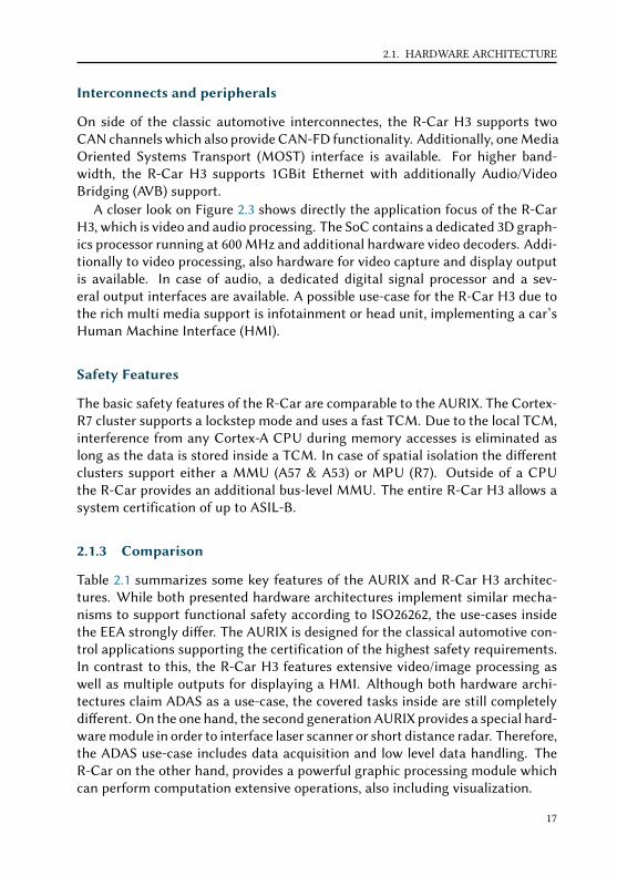
On side of the classic automotive interconnectes, the R-Car H3 supports twoCAN channels which also provide CAN-FD functionality. Additionally, one MediaOriented Systems Transport (MOST) interface is available. For higher band-width, the R-Car H3 supports 1GBit Ethernet with additionally Audio/VideoBridging (AVB) support.
A closer look on Figure 2.3 shows directly the application focus of the R-CarH3, which is video and audio processing. The SoC contains a dedicated 3D graph-ics processor running at 600 MHz and additional hardware video decoders. Addi-tionally to video processing, also hardware for video capture and display outputis available. In case of audio, a dedicated digital signal processor and a sev-eral output interfaces are available. A possible use-case for the R-Car H3 due tothe rich multi media support is infotainment or head unit, implementing a car’sHuman Machine Interface (HMI).
Safety Features
The basic safety features of the R-Car are comparable to the AURIX. The Cortex-R7 cluster supports a lockstep mode and uses a fast TCM. Due to the local TCM,interference from any Cortex-A CPU during memory accesses is eliminated aslong as the data is stored inside a TCM. In case of spatial isolation the dierentclusters support either a MMU (A57 & A53) or MPU (R7). Outside of a CPUthe R-Car provides an additional bus-level MMU. The entire R-Car H3 allows asystem certification of up to ASIL-B.
2.1.3 Comparison
Table 2.1 summarizes some key features of the AURIX and R-Car H3 architec-tures. While both presented hardware architectures implement similar mecha-nisms to support functional safety according to ISO26262, the use-cases insidethe EEA strongly dier. The AURIX is designed for the classical automotive con-trol applications supporting the certification of the highest safety requirements.In contrast to this, the R-Car H3 features extensive video/image processing aswell as multiple outputs for displaying a HMI. Although both hardware archi-tectures claim ADAS as a use-case, the covered tasks inside are still completelydierent. On the one hand, the second generation AURIX provides a special hard-ware module in order to interface laser scanner or short distance radar. Therefore,the ADAS use-case includes data acquisition and low level data handling. TheR-Car on the other hand, provides a powerful graphic processing module whichcan perform computation extensive operations, also including visualization.
17

CHAPTER 2. TRENDS IN AUTOMOTIVE ECU ARCHITECTURES
CPUs Memory Interconnects Safety use-case
AURIX 2/3x TriCore <1 MB int. RAM≤8 MB int. Flash
4x LIN6x CAN/CAN-FD2x FlexRay1x Ethernet
LockstepMPUASIL-D
GatewayDomaincontrollerEnginecontrolAirbagADAS
R-Car H34x Cortex-A574x Cortex-A532x Cortex-R7
<1 MB int. RAM≤8 GB ext. RAMext. Flash
2x CAN/CAN-FD1x MOST1x Ethernet AVB
LockstepMPU/MMUASIL-B
HeadunitInfotainmentHMIADAS
Table 2.1: SoC comparison table
Nevertheless, the R-Car H3 will never replace the AURIX within the EEA andvice versa. Both platforms have a reason for existence. The comparatively largecomputing power of the R-Car H8 is achieved by the use of performance opti-mized hardware like the integrated graphic processor or the Cortex-A clusters.The drawback at this point is, that the computation power is achieved with gen-eral purpose CPU designs, implementing techniques like speculative execution,branch prediction or out-of-order execution. Not only worsens those techniquesthe analysability and predictability, it also opens an aack space for novel ex-ploitation techniques [75]. Therefore, the R-Car H3 provides lots of computa-tion power for applications with limited safety requirements. In contrast to this,the AURIX family provides limited computation power for applications with thehighest safety requirements.
2.2 Soware Architecture
Modern automotive soware is oen developed and integrated according to theAUTOSAR [2] set of standards. This is especially the case for ECUs covered bymore classical µC architectures like the AURIX family. AUTOSAR is defined bya consortium consisting of dierent partners from the automotive industry, in-cluding automotive soware/hardware suppliers and Original Equipment Man-ufacturers (OEMs) as well as dierent research facilities. Figure 2.4 shows a sim-plified model of the AUTOSAR soware architecture. In general, it consists ofthree parts. First, the AUTOSAR Soware which contains the applications. Sec-ond, the AUTOSAR RTE which abstracts inter- and intra-ECU communication tothe application. And third the AUTOSAR Basis Soware (BSW) which integratesdriver, services and two abstraction layers.
Applications in modern automotive systems implement a car’s entire behavior.Since a few years, the development process of those applications is model based.One of the most common frameworks is Matlab/Simulink [49]. Combining thiswith automatic code generation leads to an eicient application development
18

2.2. SOFTWARE ARCHITECTURE
AUTOSAR Basic SoftwareMEM
Service
µCDrivers
AUTOSAR Runtime Environment
AUTOSAR Software
Microcontroller
I/O HAL Onboard
Device HALMEM HAL Complex
DriverCOM HAL
MEMDrivers
COMDrivers
I/ODrivers
COMService System Services
Task 1 Task 2 ... Task nTask 2
Service Layer µC AbstractionECU Abstraction
Figure 2.4: AUTOSAR Soware architecture
process where source code can be generated aer extensive simulation. Never-theless, this does not describe how the application is later executed on an ECU.We will therefore give a brief introduction in the following Subsection 2.2.1.
The RTE decouples the high-level application from the ECU specific imple-mentation of the BSW. One mechanism to achieve this is the AUTOSAR VirtualFunctional Bus (VFB) [11], which abstracts the communication between dierentapplications. Important at this point is, that it doesn’t maer if an applicationreads/writes data from/to an application on the same or a remote ECU. The VFBeither maps the access to the memory for internal communication or forwards itto the communication stack. Therefore, the VFB is described on a system level,while an actual RTE implementation on a single ECU just implements the localmapping. The data access from the application is then performed through socalled ports, providing dierent communication paradigms further described in[11]. Although the VFB perfectly decouples the application from the underlyinghardware, it is not a mandatory component of an ECUs soware. Omiing VFBand RTE reduces the abstraction overhead, which is oen the reason for this. Asa detailed knowledge of the AUTOSAR RTE is not necessary to understand themechanisms discussed aerwards, we refer to [11] for further information.
The BSW includes three dierent layers: the service layer, the ECU abstractionlayer and the µC Abstraction Layer (MCAL). Implemented services range from asimple memory management, over communication up to the system services im-plementing the OS. As this dissertation deals with scheduling mechanisms, wedescribe the classic automotive OS further in Subsection 2.2.2. Both abstraction
19

CHAPTER 2. TRENDS IN AUTOMOTIVE ECU ARCHITECTURES
100msPeriod 10msPeriod
1msPeriodElm_rDutyCycle
ElectricMotorDriver
Pdl_tqRef
Sns_iCurFlt
Elm_rDutyCycle
ControllerSns_iCur Sns_iCurFlt
Filter RateTransition1ms->10ms
Sns_iCur
CurrentSensor
Pdl_tqRef
PedalRateTransition100ms->10ms
Figure 2.5: A simple engine controller in Matlab Simulink
layers implement drivers for either ECU or µC specific components. The imple-mentation of an entire communication stack is used as an example to explainthis further in Subsection 2.2.3. Also, the temporal behavior of a communica-tion stack is important when considering scheduling techniques, as it is usuallydriven by interrupts and the application.
2.2.1 Application
Modern cars implement most of their important functionality as applications onseveral ECUs. Over the past decades remits in the automotive industry there-fore moved from pure mechanical engineering to a combination of mechani-cal, electrical and control engineering, as well as computer science. As alreadymentioned, the function development is oen based on frameworks like Mat-lab Simulink [49] enabling Model Based Design (MBD) [103]. MBD allows anabstraction to a visual functional description. Especially in case of control engi-neering MBD in combination with Matlab/Simulink is well-known, as it allowsinstant testing based on simulation. Combining MBD with automatic code gen-eration leads to an eicient application development process. Especially if thegenerated code is already compliant to the relevant safety standards [43](e.g.ISO26262).
Applications in the automotive industry are usually developed as a set of func-tions. In the terminology of Simulink, those functions are also called atomicsubsystems. An example for an application developed with atomic subsystemin Simulink is represented in Figure 2.5, showing a simple control for an electricmotor. First, the throle pedal is used as a reference input specifying a torquesetpoint. Second, the controller calculates the corresponding PWM duty cycle,which should be set by the motor driver. And third, the actual current is mea-sured and filtered in order to derive the actual torque at the drive sha. Figure 2.5
20

2.2. SOFTWARE ARCHITECTURE
fSns fElmfCtl
τ100
I fPdlfFlt
τ1
τ10
Figure 2.6: Possible runnable mapping for Figure 2.5
also shows the dierent periods (or rates) with which the corresponding func-tions are executed. In the context of an automotive embedded system, such afunction combination with a defined dataflow is called eect chain.
A well-established period for a torque based controller is 10ms [59]. In contrastto this, a user defined input like the throle pedal is executed with a greaterperiod (e.g. 100ms). Usually this is suicient, as the fastest changes for the torquesetpoint are based on human limitations. On the other hand, the actual currentvalue is provided with a smaller period (e.g. 1ms). This is oen the case as highersampling frequencies on such inputs allow more comprehensive digital signalprocessing which is cheaper compared to a pre-processing on the analog signals.Also, it might be the case that another application also uses the sampled currentvalue and is executed with a dierent period. In order to combine the dierentperiods in the model, Simulink uses rate transition blocks which provide dataintegrity during transfers between dierent periods (rates).
Generating code on a Simulink model can result in dierent high-level lan-guages for soware or hardware description. One of the most common ways inthe automotive domain is the code generation to C [71] under the considerationof dierent development guidelines [85] and safety standards [66]. The exam-ple from Figure 2.5 would generate a C-function per atomic subsystem. Withinthe automotive domain those generated C-functions are called runnables. Thoserunnables are then grouped by common periods into container tasks. The sig-nals between the dierent atomic subsystems like Pdl_tqRef or Sns_iCur resultin global variables. This way a publisher subscriber based communication is im-plemented where variables are wrien only by one runnable, but can be read byseveral other runnables.
For the example from Figure 2.5, Figure 2.6 shows a possible set of gener-ated runnabels. A container task therefore contains multiple runnables whichare executed in a static order, determined by the dataflow of the application. Inthe automotive domain the preferred task scheduling technique implemented bythe OS is preemptive and based on static priorities [13, 92], oen mentioned asStatic Priority Preemptive (SPP). Based on Figure 2.5 τ100 contains the processingof the pedal input (fPdl ). The primary control algorithm (fCtl ) and the outputdriver (fElm ) are executed in τ10. The current feedback including sensor input
21

CHAPTER 2. TRENDS IN AUTOMOTIVE ECU ARCHITECTURES
fn-1f2 f3 ...
τ
II f1 Ofn
Figure 2.7: Generic container task with n runnables and in/output processing
(fSns ) and filtering (fF lt ) is executed in τ1. This set of three periodic tasks couldnow be scheduled by an OS executing the generated code from the Simulinkmodel. τ1 would be executed each millisecond, τ10 every ten millisecond and τ100every hundred milliseconds. The priority assignment is done according to [80],assigning the highest priority to the task with the smallest period and vice versa.With a deadline equal to the task period, this is called Rate Monotonic Schedul-ing (RMS) and the most common type of scheduling (it implies SPP) in the classicautomotive domain. In general, task periods in the automotive domain are usu-ally in the range of 1ms − 500ms . Sometimes even bigger periods are used forbackground activities.
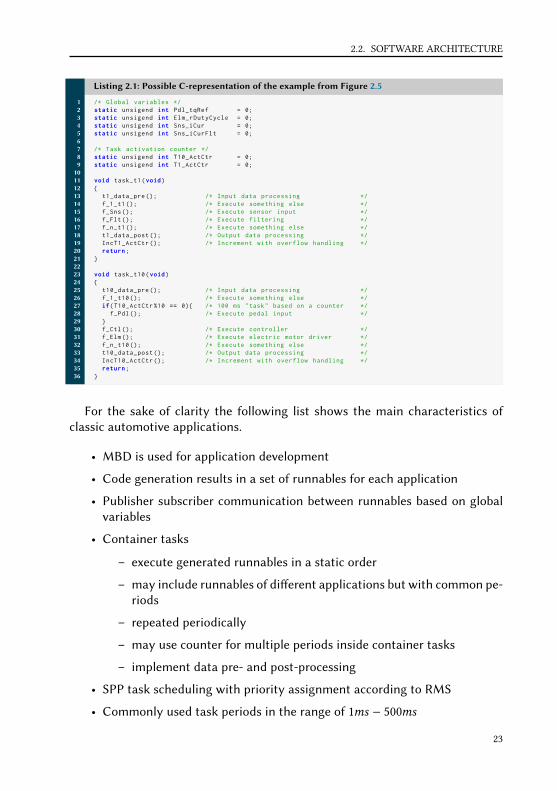
Usually an ECU implements more than one single functionality based on sev-eral Simulink models. As a result, a container task usually contains runnablesfrom multiple dierent applications. A more generic example for such a taskwith n runnables is shown in Figure 2.7. In addition to the runnables, the de-picted task τ also contains data pre- (I) and post-processing (O) oen used forscaling and local copies of global data. As already mentioned, Figure 2.6 showsa possible mapping of the generated runnables to container tasks. In some casesit might make sense to include fPdl in τ10. One possible reason for a such a mea-sure would be if the 100ms task would only contain a single runnable. To achievea period of 100ms inside the 10ms fPdl would be executed conditionally basedon a counter and a modulo operation. This way the number of tasks could bereduced, resulting in a lesser management overhead. Such an example is shownin Listing 2.1
The 10ms task is represented as task_t10 and the 1ms task as task_t1. For bothtasks, the contained runnables are executed in the shown order. The runnablefor fPdl is executed every tenth task activation based on the counter T10_ActCtr.The function IncT10_ActCtr increments T10_ActCtr as an atomic operation andimplements a task specific wrap around at the end of task_t10. In addition to that,both tasks also include calls to task specific pre- and post-processing functions(e.g. lines 12, 17, 23 and 31). The global variables in lines 2-5 implement theshown Simulink signals between the atomic subsystems and are accessed by therunnables according to Figure 2.5.
22
2.2. SOFTWARE ARCHITECTURE
Listing 2.1: Possible C-representation of the example from Figure 2.5
1 /* Global variables */2 static unsigend int Pdl_tqRef = 0;3 static unsigend int Elm_rDutyCycle = 0;4 static unsigend int Sns_iCur = 0;5 static unsigend int Sns_iCurFlt = 0;67 /* Task activation counter */8 static unsigend int T10_ActCtr = 0;9 static unsigend int T1_ActCtr = 0;
1011 void task_t1(void)12 13 t1_data_pre (); /* Input data processing */14 f_1_t1 (); /* Execute something else */15 f_Sns (); /* Execute sensor input */16 f_Flt (); /* Execute filtering */17 f_n_t1 (); /* Execute something else */18 t1_data_post (); /* Output data processing */19 IncT1_ActCtr (); /* Increment with overflow handling */20 return;21 2223 void task_t10(void)24 25 t10_data_pre (); /* Input data processing */26 f_1_t10 (); /* Execute something else */27 if(T10_ActCtr %10 == 0) /* 100 ms "task" based on a counter */28 f_Pdl (); /* Execute pedal input */29 30 f_Ctl (); /* Execute controller */31 f_Elm (); /* Execute electric motor driver */32 f_n_t10 (); /* Execute something else */33 t10_data_post (); /* Output data processing */34 IncT10_ActCtr (); /* Increment with overflow handling */35 return;36
For the sake of clarity the following list shows the main characteristics ofclassic automotive applications.
• MBD is used for application development
• Code generation results in a set of runnables for each application
• Publisher subscriber communication between runnables based on globalvariables
• Container tasks
– execute generated runnables in a static order
– may include runnables of dierent applications but with common pe-riods
– repeated periodically
– may use counter for multiple periods inside container tasks
– implement data pre- and post-processing
• SPP task scheduling with priority assignment according to RMS
• Commonly used task periods in the range of 1ms − 500ms
23

CHAPTER 2. TRENDS IN AUTOMOTIVE ECU ARCHITECTURES
CPU Core
Dispatcher
Scheduler
τ1
τ10
τ100
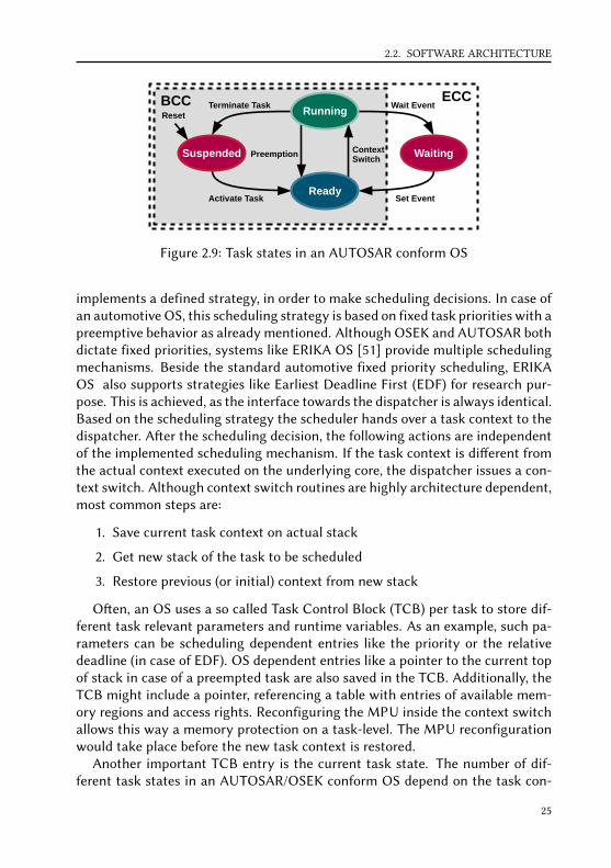
Figure 2.8: Task states in an AUTOSAR conform OS
2.2.2 Operating System
An OS is usually responsible for dierent actions. In general purpose computingthe OS oen provides multiple components including filesystems, driver and ex-tensive resource management. In the AUTOSAR context, the operating systemis considered a system service, which only provides minimal functionality. AnOS conform to the Oene Systeme und deren Schnistellen für die Elektronikim Krafahrzeug (OSEK) or AUTOSAR OS definition [13] can therefore be con-sidered as a microkernel [55, 53] design. [39] gives a good overview of the OSEKdefinition and the derived AUTOSAR OS. Primary tasks of an automotive OSare:
1. Task management
• Scheduling
• Context switching
• Memory Protection
• Conformance Classes
• Communication
• Synchronization
2. IRQ handling
• Interrupt Service Routine (ISR) types
• Alarm and counter management
The term task management bundles most of the important functions of an OS.First, the OS implements a scheduler, which determines the next task to be dis-patched. This is shown in Figure 2.8 with three dierent tasks. The scheduler
24
2.2. SOFTWARE ARCHITECTURE
BCC
ContextSwitch
Preemption
Terminate Task Wait Event
Activate Task Set Event
Running
Ready
Suspended Waiting
ECCReset
Figure 2.9: Task states in an AUTOSAR conform OS
implements a defined strategy, in order to make scheduling decisions. In case ofan automotive OS, this scheduling strategy is based on fixed task priorities with apreemptive behavior as already mentioned. Although OSEK and AUTOSAR bothdictate fixed priorities, systems like ERIKA OS [51] provide multiple schedulingmechanisms. Beside the standard automotive fixed priority scheduling, ERIKAOS also supports strategies like Earliest Deadline First (EDF) for research pur-pose. This is achieved, as the interface towards the dispatcher is always identical.Based on the scheduling strategy the scheduler hands over a task context to thedispatcher. Aer the scheduling decision, the following actions are independentof the implemented scheduling mechanism. If the task context is dierent fromthe actual context executed on the underlying core, the dispatcher issues a con-text switch. Although context switch routines are highly architecture dependent,most common steps are:
1. Save current task context on actual stack
2. Get new stack of the task to be scheduled
3. Restore previous (or initial) context from new stack
Oen, an OS uses a so called Task Control Block (TCB) per task to store dif-ferent task relevant parameters and runtime variables. As an example, such pa-rameters can be scheduling dependent entries like the priority or the relativedeadline (in case of EDF). OS dependent entries like a pointer to the current topof stack in case of a preempted task are also saved in the TCB. Additionally, theTCB might include a pointer, referencing a table with entries of available mem-ory regions and access rights. Reconfiguring the MPU inside the context switchallows this way a memory protection on a task-level. The MPU reconfigurationwould take place before the new task context is restored.
Another important TCB entry is the current task state. The number of dif-ferent task states in an AUTOSAR/OSEK conform OS depend on the task con-
25

CHAPTER 2. TRENDS IN AUTOMOTIVE ECU ARCHITECTURES
Listing 2.2: Example implementation of an BCC task
1 #define T10 1 /* Define task ID */23 TASK(T10) /* Macro based function definition */4 5 task_t10 (); /* Execute generated container task */6 TerminateTask (); /* Terminate task execution and call OS */7 return;8
formance class. Both, AUTOSAR and OSEK support two dierent conformanceclasses for tasks. So called Basic Conformance Class (BCC) tasks for executionwithout synchronization in between and Extended Conformance Class (ECC)tasks allowing synchronization during execution. In addition, both conformanceclasses can implement two dierent types of tasks. Type 1, allowing only one ac-tivation at a time per task with one task per priority and Type 2, allowing multiplequeued activations at a time per task with multiple tasks per priority. Overall thisleads to four dierent configurations based on the dierent conformance classesand dierent types (BCC1, BCC2, ECC1 and ECC2).
For the dierent task states only the conformance classes are relevant andnot the dierent types. Figure 2.9 shows the dierent states for BCC and ECCtasks. The classic automotive system does not create tasks during runtime, butuses a statically defined setup. Therefore ,all available tasks are known at sys-tem startup and each task starts in the Suspended state aer a system reset. Atask acitivation switches the corresponding task to the Ready state, indicatingthat this task can be executed. Also, scheduling decisions are only performed ontasks in the Ready state. Next is the Running state which indicates the actualexecution of the corresponding task. It is reached when a ready task is takenby the scheduler for execution and a context switch is performed through thedispatcher. Important at this point is, while several tasks might be ready for exe-cuting, only one task per CPU core can be in the Running state at a time. Whichtask is executed and therefore holds the Running state depends on the imple-mented scheduling strategy. Therefore, in case of SPP always the task with thehighest priority of all tasks in the Ready state is executed.
In case of an BCC task, the Running state can be le in two dierent ways,first based on a finished execution and second based on a preemption. For thefinished execution the task terminates itself and the task state is set to Suspendeduntil the next task activation. In case of a preemption, the task is switched backto the Ready state. This might be the case, if a task with a higher priority entersthe Ready state and is directly executed according to the scheduling strategy. Thepreviously executed task will then continue execution, until it is the task with thehighest priority in the system again. Listing 2.2 shows an example for a simpleBCC task consisting of the container task function task_t10 from Listing 2.1 andthe task termination at the end.
26

2.2. SOFTWARE ARCHITECTURE
Listing 2.3: Example implementation of an ECC task
1 #define T10 1 /* Define task ID */2 #define EV_T10 1 /* Define event ID */34 TASK(T10) /* Macro based function definition */5 6 EventMaskType mask;7 task_t10 (); /* Execute generated container task */8 WaitEvent(EV_T10 ); /* Wait for EV_T10 (enter waiting state) */9 GetEvent(T10 , &mask); /* Resume execution , get event for T10 */
10 ClearEvent(EV_T10 ); /* Clear event */11 do_something_else (); /* Do something else */12 TerminateTask (); /* Terminate task execution and call OS */13 return;14
In case of an ECC task, there is a third way to leave the Running state. As al-ready mentioned, ECC tasks allow synchronization during execution. This syn-chronization is reached through so called events which can be set by several rea-sons. In order to enable synchronization, ECC tasks implement an additionalstate called Waiting, which is entered when a task waits for an event for synchro-nization. When the corresponding event is set, the task enters the Ready stateagain. Listing 2.3 shows an example for an ECC task consisting of the containertask function task_t10, waiting for the event EV_T10, an additional function calland the task termination at the end.
Seing an event can have dierent reasons like an incoming message, syn-chronization with another task or also related to the underlying hardware throughan IRQ. IRQ handling in general is grouped by AUTOSAR and OSEK in two dif-ferent categories of ISRs. The first type ISR1 is usually not directly related to theapplication, as it does not allow access to the corresponding functions inside theOS. Instead, it is usually used for low level driver handling inside the BSW. As anISR1 does not provide any protection mechanisms, the switch to the IRQ contextand back to the previous context introduces only minor runtime overhead. Thelack of protection is the reason for the missing functionality for interaction withthe application inside an ISR1. For this purpose there is the second type calledISR2 which allows interaction with the application. This means, that e.g. from anISR2 a task can be activated or also an event can be set, which results in a directcontrol of the application from the IRQ context. This is achieved with a morecomplex switch to the IRQ context resulting in more overhead compared to anISR1. Beside the dierent ISRs, OSEK and AUTOSAR OS also support counterbased alarms for single or recurring events. Like the entire operating system,alarms are configured during design time and invoke either a task activation, setan event or call a simple callback function. For more information regarding ac-cess rights of dierent ISR types and alarm callbacks, we highly refer to figure12-1 from [92] or table 1 from [13].
27

CHAPTER 2. TRENDS IN AUTOMOTIVE ECU ARCHITECTURES
COM Drivers
x DriverSPI DriverDIO Driver
COM HAL
x Trcvx If x ExtDrv
COM Service
Generic NmCOM PDU Router
x Nmx SMx Tp
Service Layer
ECU Abstraction
µC Abstraction
Figure 2.10: Soware modules of an AUTOSAR conform COMStack
2.2.3 Soware Stacks
Another important part of an automotive soware architecture are soware stacks.Soware stacks in the context of AUTOSAR implement a set of modules verti-cally through all three layers of the AUTOSAR BSW. Considering Figure 2.4two major stacks can directly be identified. First the Communication Stack(COMStack) including COM Service, COM Hardware Abstraction Layer (HAL) andCOM Drivers, and second the Memory Stack (MEMStack) including the corre-sponding counterparts. Figure 2.10 shows the parts of an AUTOSAR conformCOMStack in more detail. The specification contains several types for in-vehiclenetworks and buses. Most common communication media types are the alreadyhighlighted technologies like, CAN, LIN, FlexRay and Ethernet. The modules inFigure 2.10 starting with an x represent multiple modules of the same type for thedierent communication media. Be aware that not all available COMStack mod-ules are shown in Figure 2.10 for complexity reasons. As an example, Figure 2.10does not show higher layer protocols like Universal Measurement and Calibra-tion Protocol (XCP) or Scalable Service-Oriented Middleware over Internet Pro-tocol (IP) (SOME/IP), although those are part of the AUTOSAR COMStack defi-nition.
Starting with the service layer, the primary interface towards the applicationor RTE is the COM module. From there on, the transmied or received valuesare mentioned as Protocol Data Units (PDUs). We will use the transmit pathin order to explain the functionality of the dierent modules. Inside the COMmodule, a multiplexing is also possible, such that a PDU might contain multi-ple dierent values. From there the PDU is passed to the PDU Router, whichdetermines the corresponding communication medium used for the final trans-mission. This means, that the PDU Router passes the PDU to the corresponding
28

2.2. SOFTWARE ARCHITECTURE
transport layer module x Tp. Inside x Tp the possible segmentation of a PDUis handled, based on the physical payload size of the underlying communica-tion medium. Additionally, the service layer includes a medium dependent statemanagement (x SM) as well as a network management (Generic Nm, x Nm). Thestate management is primarily used for stu like flow control, while the networkmanagement is responsible for protocol specific features like a bus-sleep mode.
The ECU abstraction layer primarily include the interface (x If ) and the trans-ceiver modules (x Trcv) for each communication medium. From the correspond-ing x Tp module in the service layer, an outgoing PDU is passed to specific in-terface module. Each x If represents an abstraction of the underlying hardwareto the upper service layer. This includes validity checks, transmit/reception con-firmations as well as cyclic polling of underlying hardware through the corre-sponding x Driver. Each transceiver module is responsible for the configurationof hardware modules which represent the connection to the physical layer of thecommunication medium.
The µC abstraction layer includes the needed hardware drivers (x Driver) to ac-cess the communication peripherals for data link handling. The used transceiversfor physical access of the communication media are usually o-chip and not partof the µC or SoC. Therefore, the µC abstraction layer also provides drivers fordigital in/output (DIO Driver) or the oen used Serial Peripheral Interface (SPI)(SPI Driver) in order to configure the o-chip transceivers. If the µC does notprovide a corresponding communication peripheral, it is possible to have both,physical access and data link handling, o-chip. In this case, both both o-chipcomponents may be interfaced through either digital in/output or SPI. The pe-ripheral driver for data link handling is then part of the ECU abstraction layer (xExtDrv).
AUTOSAR provides a detailed specification for each module. As an example[12] provides the specification for the COM module. For each module AUTOSARspecifies an API including type and function definitions. The API functions canbe grouped into dierent types.
First, functions relevant for module initialization and control. As an example,this contains Init/DeInit as well as GetStatus calls.
Second, a set of functions which define the API towards the upperlying mod-ules. In case of the COM module, this is the interface towards application orRTE.
Third, a set of callback functions representing the interface to underlying mod-ules. As an example for the COM module, the function Com_RxIndication is regis-tered in each x If during initialization. This way, the COM module defines whichfunction should be called when a PDU was received.
Fourth, scheduled functions. Most of the modules provide so called Main-Functions which get executed periodically from a task context. Beside the IRQ
29

CHAPTER 2. TRENDS IN AUTOMOTIVE ECU ARCHITECTURES
and callback driven functionality of the COMStack, the MainFunctions performhousekeeping and periodic PDU processing. For this purpose, the COMStackMainFunctions are oen implemented as a single task with a higher period thanthe application tasks.
From a timing perspective, a COMStack therefore introduces two dierenttypes of load to a system. On the one hand the IRQ driven processing oen basedon low level driver handling, and on the other hand, the periodically executionof the MainFunctions. For an application, both can be considered as interferenceas those COMStack modules are executed on a higher priority.
2.2.4 Adaptive AUTOSAR
The previously described application model and system architecture from Sec-tion 2.2 is well-known and has proven itself in recent years. Nevertheless, thissoware architecture does not fit the needs for all future use-cases. Featureslike highly automated driving as part of ADAS, car2x communication or par-tial updates over the air are one of the most important technology drivers oftoday’s automotive industry [50]. Primarily, highly automated driving requiremore powerful ECUs for local sensor fusion and processing. But also, the con-nection to backend servers get more important in order to receive something likecurrent or predicted traic data for route planning [88]. This way a car gets moreand more connected to its surrounding environment and the internet. As alreadyshown in [84], this steady connection can be exploited if it isn’t done properly.The existing procedure, where an ECUs soware is only updated in a verifiedgarage, is acceptable for systems which are not remotely accessible. Comparedto this, in case of an always connected system updates must be applied as soonas possible. Otherwise, the car would be prone to security leaks, which indirectlycould endanger the passengers safety (e.g. [84] pages 83-86). Patching securityleaks remotely over the air without having the car taken to the garage, is there-fore the way to go. Also, via an over the air update additional functionality canbe enabled at later date.
Again, those mentioned features are not compatible to the existing set of stan-dards. One big reason for this is, that the existing AUTOSAR standards don’t al-low reconfiguration or partial updates during runtime. Therefore, the AUTOSARconsortium decided to provide another set of standards called AUTOSAR Adap-tive Platform (AP) and rename the existing specification to AUTOSAR ClassicPlatform (CP). Important is at that point, that the AP is not meant to be a re-placement of the CP. Systems of both standards should be able to coexists sideby side in the same EEA, on the same ECU or also on the same µC/SoC. Table 2.2shows the main dierences between both, CP and AP.
First of all, the OS of the AP is no longer based on theOSEK specifications.
30

2.2. SOFTWARE ARCHITECTURE
AUTOSAR CP AUTOSAR APOS OSEK POSIX
MemoryManagement Only MPU for safety Virtual address space per application
with an MMU
CodeExecution
Statically from Read Only Memory(ROM)/Flash
Dynamically loaded to RAM during run-time
TaskScheduling
Fixed number of tasks, scheduling basedon priority
Dynamic number of tasks, dierentscheduling mechanisms
CommunicationProtocols Signal based (CAN,FlexRay etc) Service oriented (SOME/IP)
ExemplaryHardware AURIX R-Car H3
Table 2.2: Comparison table of the AUTOSAR CP and AUTOSAR AP based on[21]
Instead, a minimal subset (PSE51 [14, 16]) of the POSIX standard [113] is used,defining an API between applications and OS. There are several OSs available,which are either certified or mostly compliant to the POSIX standard. Due to itsopen source format and wide hardware support, Linux [19] is one possible OSfor the AUTOSAR AP [88]. Receiving updates over the air requires a MMU in or-der to provide multiple memory address spaces. Reason for this is the fact, thatduring compile time the physical address where the final binary is later placed,can not be determined. Instead, applications or updates are linked to a fixed andconstant memory layout, which is later provided by the MMU. Each applicationis executed in its own virtual address space. As a result of this technique, ap-plications are not executed from the ROM/Flash anymore, but loaded into theRAM beforehand. As task scheduling and configuration belongs to the operatingsystem, the AP supports several dynamic mechanism defined by POSIX [118]. Ingeneral, an application is not stuck to a fixed number of tasks anymore. Ac-cording to [14], the first supported scheduling algorithms are SCHED_FIFO andSCHED_RR, as defined by POSIX. Nevertheless, first measurements show that aLinux based AP struggles with reaching the same hard real-time behavior com-pared to a much slower CP [67]. The communication between dierent ECUsis limited to SOME/IP in case of an AP. As already mentioned, the AUTOSARCOMStack supports SOME/IP as a higher layer protocol. This way the commu-nication between CP and AP ECUs is ensured. Also, this way the AP gets accessto the existing in vehicle network. We already mentioned that the dierent hard-ware architectures explained in Section 2.1 are both relevant for modern ECUs.Both hardware architectures were chosen as examples for good reason. The AU-RIX is a well-known and widely used µC for ECUs based on the AUTOSAR CP.
31
CHAPTER 2. TRENDS IN AUTOMOTIVE ECU ARCHITECTURES
The R-Car H3 as an SoC instead fits perfectly into the profile of an AUTOSARAP ECU.
With the first definition of the AP, AUTOSAR also introduced the possibilityof virtualization through a hypervisor [16]. The execution of multiple AP or evenCP instances on the same SoC are therefore considered a possible integrationby the AUTOSAR consortium. According to ISO26262, the hypervisor is then incharge of preserving freedom from interference between dierent AUTOSAR APor CP instances. Although the standardization is in an early stage of progress atthe moment, dierent soware suppliers in the automotive industry are workingon actual hypervisor implementations [88, 30]. As already mentioned, futurehardware platforms like the R-Car H3 already provide hardware mechanisms tosupport virtualization.
2.3 Problem Statement
With the introduction of the AURIX µC family, the evolution of multicore CPUsreached the automotive industry. While the AURIX is primarily targeted to theCP, same applies to the newly developed AP with SoCs like the R-Car H3. Forboth platforms an eicient use of the available processing power is key to a goodoverall performance. Dependent on the platform type, the limiting constrainsfor eicient use of the available resources vary. On both AP and CP the parallelexecution and synchronization among multiple cores of existing legacy sowareis a big issue and needs to be addressed. Also important is, the application map-ping to dierent cores, as well as the freedom from interference between thoseapplications. As an example, [86] proposes a mapping where on core does onlycontain periodically executed applications. Non periodic soware like IRQ han-dling is then executed on another core. While this oen can hardly be reached, italso isn’t always useful to completely decouple periodic and sporadic executionon dierent cores due to latency issues.
2.3.1 Eicient Hypervisor Scheduling
The AP paves the way for much more powerful ECUs which can be used for eitherinfotainment or also computing intense operations in ADAS. Nevertheless, theeicient use of such SoCs is still challenging, as parts of dierent applicationsneed to be mapped to the available cores. Figure 2.11 shows a mapping based onan example described in [88]. The ECU in Figure 2.11 contains two dierent typesof CPU cores. A set of performance cores and a set of safety cores. The R-CarH3 could be a possible SoC for such a setup with Cortex-A covering performanceand Cortex-R safety tasks. The safety cores are used for system monitoring andtherefore execute an AUTOSAR CP. Contrary to this, the performance cores are
32

2.3. PROBLEM STATEMENT
Performance Cores
ECU
HypervisorSafety Cores
ClassicPlatform
VMClassic
Platform
vCores
VM
vCores
AdaptivePlatform
Figure 2.11: Mixed soware mapping with AP and CP
under the control of a hypervisor executing two dierent AUTOSAR instances.In this mapping an AP would execute the primary application. As the AP onlyprovides SOME/IP for communication, an additional CP is used to connect theECU to the common interconnects like CAN, FlexRay or LIN.
In such a configuration the hypervisor provides virtual CPU cores (vCores)to the upper soware layers. In other words, the hypervisor provides a VirtualMachine (VM) to each AUTOSAR instance. Each VM might contain multiple vir-tual cores. How the virtual cores are mapped to the available physical cores ismanaged by the hypervisor. Same applies to the translation between virtual andphysical memory addresses. When multiple virtual cores are mapped to the samephysical core, the hypervisor acts as a resource arbiter. From the perspective ofthe hypervisor, the dierent virtual cores can be interpreted as tasks scheduledon a physical core. Result of this technique is a hierarchical scheduling contain-ing hypervisor level and OS level task scheduling. At this point it is importantto mention that, even though the AP considers hypervisor based virtualizationto be a possible way to integrate dierent applications on the same hardware, itdoes not provide any definition about the actual integration. Therefore, a formaldefinition on how the hypervisor level scheduling should be integrated is missingcompletely.
While being fairly new in the automotive domain, hierarchical scheduling iswell-known in avionics as part of ARINC653 [93]. We already mentioned PikeOS[70] as an example for a well-established OS and virtualization environment inavionics. In order to provide temporal isolation among multiple VMs, ARINC653uses a time partitioning with TDMA. This means, that partitions (VMs) get exe-cuted by the hypervisor cyclically in a fixed order for fixed amounts of time. As aresult, each partition is executed for a fixed amount of time within a certain pe-riod, independent of the behavior of any other partition. While TDMA providesa perfect temporal isolation this way, the scheduling isn’t work conserving. This
33

CHAPTER 2. TRENDS IN AUTOMOTIVE ECU ARCHITECTURES
means, that the processor can be idle (because the current partition is idle), eventhough another partitions has outstanding workload. At this point processingpower is wasted and response times of task or IRQ inside partitions rise. Thisentire behavior is explained further more in Chapter 4.
Since IRQs are an essential part of the existing autmotive soware architec-ture for soware stacks or applications, longer response time are particularlybad. In case of avionics, those problems can be solved with a faster and more ex-pensive processor. For a high volume market like automotive, wasting processingpower is not applicable. As a result, a new work conserving scheduling for thehypervisor is needed. In order to enable freedom from interference (as requiredby ISO26262), a suicient degree of temporal isolation must be ensured.
Requirements
We address the previously described issue according hypervisor scheduling un-der the following requirements. The proposed mechanism should provide:
1. Work-conserving scheduling
2. Improved response times
3. Suicient degree of temporal isolation
4. Low overhead implementation
Proposed solution
In order to provide the required isolation as part of an eicient hypervisor schedul-ing, we propose a modification of the partition based scheduling described inARINC653. Chapter 4 gives an introduction to ARINC653 and highlights firstissues. Chapter 5 proposes our final scheduler modification based on the SPSmechanism. The implementation is then extensively explained in Section 7.1.
2.3.2 Multicore Synchronization
As already mentioned, a major problem during the migration to multicore ECUsis the eicient usage of the additional cores for existing legacy soware. Reasonfor this is the fact, that most of the soware has been developed for singlecoreECUs. Oen, single soware parts (e.g. runnables) have proven themselves andwere not been touched the past years. Tearing them apart and distributing themto dierent cores can cause major problems due to data inconsistencies. What’ssurprising is that less interference by other soware parts can be a problem.
Figure 2.12 provides an example for clarification. Let us assume an eectchain, where input data (green arrow) is first processed by τ10. The intermediate
34

2.3. PROBLEM STATEMENT
τ10C
0
0 10 20
τ10
τ20
t
τ10
End-to-end Latency
(a) Singlecore implementation
τ10C
0
0 10 20
C1
τ10
τ20
t
τ10
End-to-end Latency
(b) Multicore implementation without interference
τ10C
0
0 10 20
C1
τ10
τ20
t
τ10
Input Jitter
(c) Multicore implementation with interference
Figure 2.12: Task distribution from single- to multicore
data (orange arrow) is then passed to τ20 where the final data (blue arrow) is gen-erated. For this final data, the output (red arrow) is then generated in τ10. Sucha setup is very common in the automotive domain. τ10 can be interpreted as theperiodic COMStack task which connects the application tasks to the in-vehiclenetwork. The application is then implemented as part of τ20.
Figure 2.12a shows this for a simple singlecore (C0) implementation. τ10 isactivated and executed every 10ms . Same applies to τ20 every 20ms starting withan oset at t = 10ms . Due to the priority assignment based on RMS, τ10 has ahigher priority than τ20. Therefore, τ10 is always executed first, even though τ20was activated at the same time. This way the RMS-based priority assignmentsupports the desired dataflow, as both tasks are scheduled and executed on thesame core. The time between processing the first input data (green arrow) andproducing the final result (red arrow) is mentioned as an eect chains End-to-endLatency.
35

CHAPTER 2. TRENDS IN AUTOMOTIVE ECU ARCHITECTURES
On a system with multiple cores this might not be the case anymore. Fig-ure 2.12b shows an example where τ10 and τ20 are mapped on dierent cores. Areason for this might be the aempt to isolate the COMStack on a distinct core.This way the interference to the application caused by IRQs and the periodicallyexecuted MainFunctions would be removed. While the priority based schedulingdelayed the execution of τ20 in the singlecore implementation, this is not the casefor the shown multicore implementation. Without the interference from τ10, τ20starts execution immediately at t = 10 on core C1. As τ10 is executing in par-allel on C0, τ20 will read its input value before the newest value was wrien bythe current instance of τ10. Instead, τ20 reads the value wrien by the previousinstance of τ10 activated at t = 0. This way the application in τ20 is working onolder input data, which directly increases the end-to-end latency.
In the provided example in Figure 2.12b τ20 is working on older input datacompared to the singlecore implementation from Figure 2.12a. If such an inputdelay is acceptable or not depends on the underlying application soware. Also,methods like model based prediction can be used if the input delay is constant.However, a problem arises if the input delay is not constant. As an exampleFigure 2.12c shows the same task mapping as Figure 2.12b but introduces addi-tional interference on C1. Reason for the additional interference can be anothertask with a higher priority, IRQ handling or an application task with VariableRate-Dependent Behavior (VRB) [38]. Such VRB tasks can be found in ECUs forcombustion engine control, where at least one task is activated based on the ro-tation of the cranksha. Due to the interference the execution of τ20 is delayedin such a way that it starts aer τ10 has finished execution on C0. This way τ20reads the most recent value like in Figure 2.12a resulting in the same end-to-end latency. In case of a sporadic interference, the execution of τ20 is not alwaysdelayed and therefore the previous input value is read (dashed orange arrow).As a result of this behavior, the input delay can not be considered as constantanymore because of the so called input jier. The authors in [106] showed ina simple example that even a small input jier might cause serious problems.In some cases it may even lead to an unwanted instability of the implementedcontrol algorithm [90].
Even though the used example in Figure 2.12 shows a perfect example for theCP, same applies for the coordination between dierent cores in a virtualized en-vironment. Therefore, the same behavior can be expected when executing entirevirtualized partitions on dierent cores without synchronization, as part of anAP integrated system.
36

2.3. PROBLEM STATEMENT
Requirements
We address the previously described issue according synchronization of legacysoware across multiple cores, under the following requirements. The proposedmechanism should provide:
1. Comparable end-to-end latency relation to singlecore
2. Minimized input jier
3. Low overhead implementation
Proposed solution
In order to address the previous requirements, we take a look in this disserta-tion at the LET paradigm. Chapter 6 provides a basic explanation as well as thetheoretical foundation. The implementation is then extensively explained in Sec-tion 7.2.
37

CHAPTER 2. TRENDS IN AUTOMOTIVE ECU ARCHITECTURES
38

CHAPTER3
System Model
“So, in the face of overwhelming odds, I’m le with onlyone option: I’m going to have to science the shit out of this.”
- Mark Watney
This chapter presents the used system model for the underlying RTA. We providethe formal foundation for both challenges from Section 2.3. But, in order not toanticipate too much, mechanism specific system aributes will be introduced inthe corresponding chapter. Even though the RTA for the proposed mechanismsuses the same framework, there are, however, significant dierences. This chap-ter uses therefore more generic definitions, which fit the proposed mechanismsof both challenges from Section 2.3.
In general the topic of extensive RTA has been well-known for years. In orderto guarantee real-time properties suitable frameworks are Compositional Per-formance Analysis (CPA) [58] or Real-Time Calculus (RTC) [114]. As a part ofLuxso, Symtavision provides with SymTA/S a commercial CPA implementation[81]. Beside SymTA/S, Python Implementation of Compositional PerformanceAnalysis (pyCPA) [40] provides an open source CPA implementation. Within thisdissertation we use CPA as a framework in order to show the formal benefits ofour mechanisms. The used system model is based on [110, 17, 87]. While CPAis capable of system level analysis, we focus on the local resource analysis. Ourmodel is therefore slightly modified and reduced compared to the one used in[110, 17, 87]. We start with a structural platform definition, provide an executionmodel and explain the fixed-point iteration of the used RTA.
39

CHAPTER 3. SYSTEM MODEL
Definition 3.1: Platform
A platform P is defined as a directed graph
P = 〈R, E〉 (3.1)
with R as vertices, representing a set of m resources R = ϕ1 . . .ϕm. E ⊆(ϕa,ϕb ) : ϕa , ϕb ∈ R are the edges of the directed graph which defineconnections between dierent resources.
Such resources might be a CPU core, an interconnect or also an interface to ashared memory. Within the context of this dissertation, we consider only CPUcores as resources.
Definition 3.2: Resource
Each resource ϕi ∈ R is defined as
ϕi = Γi ,Si ,bi (t) (3.2)
with Γi = τ1 . . . τm as s set of m tasks, Si as scheduler for resource arbi-tration and bi (t) as service function.
3.1 Execution Model
In general, a resource provides service to a set of tasks. Service allocation tothe dierent tasks is managed by the implemented scheduling strategy. Theexecution model defines, how the provided service is consumed by the tasks. Asalready mentioned in Section 2.2.1, tasks implement the actual application. Thefollowing parameters can therefore directly be derived from the correspondingapplication.
Within the domain of real-time systems usually the average-case performanceis negligible. More important instead are bounds for best- and worst-case behav-ior. The following definitions are therefore tailored to fit the best-/worst-caseanalysis.
40

3.1. EXECUTION MODEL
Definition 3.3: Task
A task τi is defined as
τi = ET i , EMi ,TPi ,Di (3.3)
with ET i defining execution time bounds, EMi as event model, TPi asgeneric task parameter and Di as relative deadline.
The generic task parameter depends on the used scheduling strategy. As anexample, in case of a priority driven scheduling it holds the task priority. For atime driven scheduling like TDMA the parameter would represent the timeslotsize.
In order to perform any kind of action or calculation, a task needs to consumeservice on the corresponding resource. In case of CPU cores, this received serviceis called execution time. Due to the behavior of complex soware, this executiontime is oen not constant for consecutive activations of the same task. Onereason for this is conditional execution based on if-statements (e.g. Listing 2.1line 27). The execution time model therefore provides bounds for minima andmaxima.
Definition 3.4: Execution time
The execution time model ET i is a tuple with two entries
ET i = Ci ,Ci (3.4)
where Ci is the best-case (Best-Case Execution Time (BCET)) and Ci theWorst-Case Execution Time (WCET) of τi .
Beside the dierent execution times, we also need to model task activations.A common method is to describe multiple task activations as a stream of events,where each event corresponds to one task activation. Within the time domainthis stream has an infinite length. An event model uses a set of parameters todescribe the behavior of such a stream in a formally. As an example, Figure 3.1ashows an event stream for a periodically activated task. Each perpendicular ar-row indicates an event and therefore a task activation. The parameter P definesthe period used for event triggering. In order to provide a more versatile model,an additional jier J can be introduced allowing an event to occur with a speci-fied region. This is shown in Figure 3.1b. In case of J ≥ P , the specified regions inwhich an event can occur per period overlap. In order to avoid multiple events atthe same time a minimum distance dmin between two consecutive events can bedefined as shown in Figure 3.1c. This way also bursts of multiple events can be
41

CHAPTER 3. SYSTEM MODEL
tP P
(a) Periodic
tP P
J J J
(b) Periodic with jier
tP
JJ J
P
dmin
(c) Periodic with jier andminimum distance
Figure 3.1: P, PJ and PJd event model
modeled. The three shown examples are named according to their parametersas P, PJ or PJd event model. Also, [99] describes several other event models likesporadic or sporadically periodic events.
Definition 3.5: Event model
The EMi of τi is given as
EMi = EPi ,ηi , δi (3.5)
where EPi is a set of parameters describing EMi in the time domain. ηiand δi are derived sets of functions, describing bounds on EMi in the timewindow domain.
While EPi represents the event model’s parameter set, additional functions forevent bounds are needed for the later discussed RTA. Instead of an infinite eventstream, the RTA only considers time windows starting at the so called criticalinstant [80] .
Definition 3.6: Critical instant
The critical instant defines that the worst-case interference to τi is caused,when all interfering tasks are activated at the same time as late as possibleaccording to their event model. All subsequent activations arrive then as earlyas possible. According to [80] this results in the worst-case response time ofτi .
According to the critical instant, arrival and distance functions are then definedas:
42

3.1. EXECUTION MODEL
Definition 3.7: Arrival functions
ηi is a set of arrival functions
ηi = η−i (∆t),η
+i (∆t) (3.6)
where η−i (∆t) returns the minimum number and η+i (∆t) the maximum num-ber of events for τi that can arrive within any time window of size ∆t relativeto the critical instant.
Definition 3.8: Distance functions
δi is a set of distance functions
δi = δ−i (q), δ
+i (q) (3.7)
where δ−i (q) returns the minimum distance and δ+i (q) the maximum betweenthe first and the q′th consecutive event of τi , where the first event occur atthe critical instant.
The distance functions are therefore a dual representation of the arrival func-tions. E.g. η+i corresponds to δ−i , while η−i corresponds to δ+i and vice versa.
Both, arrival and distance functions can be derived from EPi . As an example,for the shown PJ model from Figure 3.1b EPi is given as:
EPi = Pi , Ji (3.8)
Under consideration of the critical instant, the corresponding arrival and dis-tance functions are derived to:
η−i (∆t) =
⌊∆t + J
P
⌋, η+i (∆t) =
⌈∆t + J
P
⌉(3.9)
δ−i (q) = (q − 1) · P − J , δ+i (q) = (q − 1) · P + J (3.10)
As [99] provides a detailed explanation how, either arrival or distance functionscan be constructed based on the corresponding event model parameter set, wewon’t discuss this step in further detail. In order to provide a more elegant no-tation, we define EMP (P), EMP J (P, J ) and EMP Jdmin (P, J ,dmin) as functionsreturning a corresponding event model for a P, PJ or PJd task.
One big dierence between real-time and none real-time systems is the exis-tence of an actual task deadline.
43

CHAPTER 3. SYSTEM MODEL
Definition 3.9: Relative deadline
The deadline Di defines the latest possible time at which an activation of τimust be finished relative to the corresponding event, responsible for activatingτi .
Without a deadline an important constraint would be missing, as it is crucialfor the functional correctness of an application. As an example, the functionalcorrectness of an airbag ECU is not only defined by the task of triggering theairbag. The task must be finished in a strictly defined period, as otherwise thepassengers face might hit the steering wheel.
Knowing the execution model of a task, we can derive several additional defi-nitions to characterize tasks, resource and scheduler further more. In some casesit makes sense to provide a rough estimation in order to estimate a task-setsschedulability.
Definition 3.10: Laxity
The laxity Li of τi is defined as
Li = Di −Ci (3.11)
As shown above, the laxity depends only on the WCET and the relative deadline.Both parameters either depend on the resource and/or the application. The in-formation value give by the laxity is torn. While Li < 0 indicates that τi can notbe scheduled on the corresponding resource, the opposite does not necessarilyapply for Li ≥ 0. Important is, that the laxity does not consider any interferenceduring execution. It is therefore independent of the underlying scheduler andthe residual set of tasks on the resource.
Also, the current state of a resource is relevant for analysis as well as later forscheduler implementation. We therefore define two dierent states. The first isgiven as:
Definition 3.11: Busy
A resource ϕi is considered as busy as long as at least one of the tasks in Γiis processing an activation on ϕi .
With this definition we define the second state as:
Definition 3.12: Idle
A resource ϕi is considered as idle if it is not busy.
44

3.2. RESPONSE TIME ANALYSIS
As already stated in Section 2.3.1, one objective of this dissertation is a work-conserving scheduling. For unambiguity, we define work-conserving based onDefinition 3.12 as follows.
Definition 3.13: Work-conserving
A scheduler Si is considered as work-conserving, when ϕi is only idle, if noneof the tasks in Γi has an unfinished activation.
3.2 Response Time Analysis
With the execution model complete, we can now explain the actual RTA. [80] isoen mentioned as one of the most popular and earliest publications concerningthe schedulabilty of task-sets. The proposed theorems in [80] provide a simpleestimation based on the utilization of the entire task-set. This was possible as thetasks were limited by a simple periodic event model with deadlines equal to theirperiods. We already mentioned this type of scheduling as RMS. As a result, theproposed theorems provide a simple boolean statement about the schedulablityof the task-set without giving any information about the actual task responsetimes.
Definition 3.14: Response time
The response time is defined as the time between activation and terminationof the task including all preemptions by other tasks. RT i defines a tuple withtwo entries
RT i = Ri ,Ri (3.12)
where Ri is the best-case (Best-Case Response Time (BCRT)) and Ri theWorst-Case Response Time (WCRT) of τi .
A well-known method to compute WCRTs is the busy-window analysis in-troduced in [69]. General idea is to compute the time, the resource is busyprocessing an activation of the considered task and its interferes. In [69], thismethod was again limited to RMS with implicitly defined deadlines at the endof each period. Later in [78] the busy-window method (busy period in this paper)was modified in order to handle arbitrary deadlines. When considering arbitrarydeadlines, queued task activations may occur. This might be the case for a taskwith periodic activations but D > P . In order to deal with this, [78] defined thelevel-i busy period, starting with the critical instant. The authors proofed that
45

CHAPTER 3. SYSTEM MODEL
the longest response time during that period corresponds to the WCRT. Withthe already mentioned arrival and distance functions, [104] modified the busy-window method in order to handle arbitrary task activation paerns. The resultwas the definition of the multiple event busy-window (busy-time in [104]). Im-portant is at this point, that the busy-window method in general is only definedto be applicable on work-conserving schedulers. This also holds for the later de-fined multiple event busy-window.
Primarily the busy-window technique was developed for priority based schedul-ing like RMS or SPP. In [104] the multiple event busy-window wi (q) of the q’thwas given as
wi (q) = q ·Ci +∑
τj ∈hp(i)
η+j (wi (q)) ·C j (3.13)
withhp(i) as set of interfering tasks with a higher priority than τi . Aswi (q) occuron both sides of the equation, wi (q) must be calculated several times
w0i (q) = 0
w1i (q) = q ·Ci +
∑τj ∈hp(i)
η+j (w0i (q)) ·C j
. . .
wni (q) = q ·Ci +
∑τj ∈hp(i)
η+j (w(n−1)i (q)) ·C j
until a fixed-point is reached (wni (q) = w (n−1)
i (q)). While q ·Ci only depends onthe analysed task, the sum on the right depends on the priority based schedulingstrategy. In order to provide a more generic definition, we replace the sum witha simple blocking term. Within this dissertation we define the multiple eventbusy-window as follows:
Definition 3.15: Multiple event busy-window
The q-event busy-window wi (q) is given as the time needed to process q ac-tivations of τi ,
wi (q) = q ·Ci + Bi (wi (q)) (3.14)
where Bi (∆t) is the caused interference by other tasks on the same resource.
Bi (wi (q)) is then defined for each scheduling strategy separately. To determineRi of τi , the first Qi activations of τi have to be considered.
46

3.2. RESPONSE TIME ANALYSIS
Qi = max(n : ∀q ∈ N+,q ≤ n : δ−i (q) ≤ wi (q − 1)
)(3.15)
A more intuitive description is, that the (q + 1)′th activation must be consideredif it occurred during the busy-window of the first q activations [78]. The worst-case response time is then given as the maximum of all observed response timesof the analysed task during the multiple event busy-window. The earliest q′thactivation relative to the critical instant is given through the minimum distancefunction δ−i . With the corresponding window size of theq′th activation this leadsto:
Ri = maxq∈[1,Qi ]
(wi (q) − δ
−i (q)
)(3.16)
With knowledge of the WCRT, we can define the schedulablity of an entiretask-set.
Definition 3.16: Schedulability
A set of tasks Γi is considered as schedulable if all tasks have WCRTs loweror equal their relative deadlines
Γischedulable ⇔ ∀τj ∈ Γi : R j ≤ D j (3.17)
Compared to the provided mechanisms in [80], a scheduleability definition basedon actual WCRTs is more computationally intensive but independent of the usedscheduling mechanism and not restricted to RMS.
We already introduced the laxity in Definition 3.10 and mentioned that ad-ditional interference is not taken into account. This is dierent in case of taskslack.
Definition 3.17: Task slack
The slack Si of τi is defined as
Si = Di − Ri (3.18)
Task slack is calculated based on WCRT and deadline. It therefore includesscheduling based interference by other tasks and provides an information aboutthe flexibility of the task-set. In case of a larger task slack, the task can be de-layed for a certain amount of time without missing its deadline. This can be
47

CHAPTER 3. SYSTEM MODEL
very useful since it allows subsequent changes. This knowledge is later used forsystem optimization through scheduling modifications.
48
CHAPTER4
ARINC653 based Hypervisor Scheduling
“I’m a leaf on the wind. Watch how I soar!”
- Hoban Washburne
Since a few years virtualization has becomme more and more relevant, also withinthe world of embedded systems. Modern CPUs like the introduced R-Car H3provide additional hardware in order to support virtualization eiciently.
As mentioned in Section 2.3.1 we consider ARINC653 a possible basis for themechanisms needed to ensure freedom from interference between dierent ap-plications on the same ECU. The remainder of this chapter shows, how ARINC653achieves the mentioned temporal isolation among its virtualized partitions. Wealso highlight the drawbacks of this approach regarding IRQ and task responsetimes. To mitigate these problems we provide a possible modification to the hy-pervisor scheduling and discuss its pros and cons. Most of the contribution inthis chapter has been published before in [28, 23].
4.1 System model addition for hierarchical scheduling
The scheduling in ARINC653 is hierarchically structured based on TDMA andSPP. An example with two partitions (P1 & P2) is given in Figure 4.1. The hyper-visor executes the dierent partitions aer each other and repeats this cyclically.Inside a partition the tasks of the virtualized application are scheduled preemp-tive based on their priorities. A task can therefore be disturbed during execution
49

CHAPTER 4. ARINC653 BASED HYPERVISOR SCHEDULING
P2P1
t
Prio
System Idle
Task activation Task preemption
Hig
hM
edL
ow
Figure 4.1: ARINC653 inspired scheduling
for several two reasons. First, it is preempted based on interference inside thepartition caused by another task of the same application. And second, the par-tition itself is at the end of its timeslot and the hypervisor switches to the nextpartition in the TDMA schedule. Also, Figure 4.1 shows the major drawback ofTDMA based scheduling. It is not work conserving. At two points during theexecution of P1 the system is idle, as none of the tasks in P1 has an outstandingactivation. In contrast to this, the medium priority task in P2 would be ready toexecute.
In order to describe such a hierarchical system formally, we need an additionto the system model described in Chapter 3. For the extended model a task-set Γp with multiple tasks is mapped to a partition Pp . A partition-set ΓHYP withmultiple partitions is then mapped to a resource. The number of partitions insideΓHYP is denoted by Ω. According to Definition 3.3 we need to adapt the parti-tion parameters to the given task model. While each partition always containsan additional task-set for the POS, other parameters depend on the schedulingstrategy used by the hypervisor. In case of TDMA each partition Pp has a timeslotwith sizeTp . The partitions are executed in their corresponding timeslots with astatic order repeated every TTDMA.
TTDMA =∑
p∈ΓHYP
Tp (4.1)
As shown in Figure 4.1 the actual used time for task execution inside a partitiondoesn’t have to be the same compared to the size of the corresponding timeslot.In order to handle this in formal way, we define Tp,min as the minimum timeneeded during the timeslotTp in order to finish all partition internal tasks beforetheir deadlines. A result of this observation is the so called partition slack.
50

4.1. SYSTEM MODEL ADDITION FOR HIERARCHICAL SCHEDULING
T1 T2 T3 T4
TTDMA
TTDMA-T1
Δt = TTDMA
IRQ/Task Activation
Figure 4.2: Temporal isolation in any time window of size TTDMA
Definition 4.1: Partition slack
The partition slack Tp,S is given as the time, which is not necessary neededby the task-set Γp inside in order to reach all deadlines.
Tp,S = Tp −Tp,min (4.2)
A way how Tp,min can be calculated is shown later in Section 4.5. With Tp,mindefined, we can now describe a partition under TDMA scheduling based on Def-inition 3.3. From the perspective of the hypervisor the caused interference by apartition Pp can be considered as a periodic task τp with periodTTDMA andTp asexecution time. In order to calculate the multiple event busy-window for a taskτi inside a partition Pp , we simply rewrite the equation from Definition 3.15 to
wp,i (q) = q ·Cp,i + Bp,i (wp,i (q)) (4.3)
where Bp,i (∆t) includes both, the blocking caused by the hypervisors and thepartition internals scheduling strategy.
We already mentioned that temporal isolation is given, if the response timeof a task is independent of the behavior of all other tasks on the same resource.While we can describe a partition as an interfering task, we can not directlydefine a response time for a partition. Another definition can be derived whenconsidering the received service and the caused interference to a task in a specifictime window. An example, how this can be derived, is shown in Figure 4.2 repre-senting a setup with four time partitions. The scheduling is fixed and repeatedeachTTDMA time units. If we start on the le, P1 is scheduled first. AerT1 timeunits P1 is preempted for TTDMA −T1. Within the first TTDMA time units the re-ceived service of each Pp isTp and the received interference isTTDMA −Tp . If weconsider a time window of size TTDMA and move it across the shown schedule,the received service as well as the received interference is always the same. Weget therefore for any time window of size TTDMA the following received servicebp and received interference Ip :
51

CHAPTER 4. ARINC653 BASED HYPERVISOR SCHEDULING
bp (∆t = TTDMA) = Tp (4.4)
Ip (∆t = TTDMA) =∑
j ∈ΓHYP \p
Tj = TTDMA −Tp (4.5)
Both values only depend on static parameters of the TDMA scheduling andnot on the behavior of another partition. This leads us to the following genericdefinition of temporal isolation.
Definition 4.2: Temporal isolation
A scheduler Si provides temporal isolation to a task τj on ϕi if
I Sij (∆t) = f I (∆t, τj ,Si ) (4.6)
bSij (∆t) = fb (∆t, τj ,Si ) (4.7)
where both the received interference I Sij (∆t) and the received service bSij (∆t)on ϕi only depend on the size of the considered time window ∆t , the usedscheduler Si and the considered task τj . The behavior of any other task τk ∈Γi \ τj on ϕi does not have any eect on I Sij (∆t) or bSij (∆t).
4.2 IRQ handling in virtualization environments
While the non work conserving scheduling with strict partitioning is already lessthan optimal for tasks, it gets even worse for IRQs which usually require partic-ularly short response times. Access to the interrupt controller of the underlyinghardware is only possible from the hypervisor. Otherwise, spatial as well as tem-poral isolation might be violated. As result, the POS does not directly interactwith the physical interrupt controller but with a virtualized instead. How this vir-tutalized interrupt controller is implemented depends on the used so- as wellas hardware. As an example, [41] uses a soware based IRQ virtualization bymeans of queues. Since hardware support for virtualization was integrated intomodern architectures, the usage of a second virtualized register shows a hard-ware based integration [10]. Nevertheless, both methods behave similar whenprocessing IRQs in a hypervisor.
Modern operating systems like Linux divide the IRQ processing in dierentparts, executing dierent tasks on dierent access layers. In case of Linux, theso called Top Half (TH) is executed directly in the ISR and is responsible for pe-riphery dependent actions. This may include reseing IRQ flags as well as re-configuring hardware registers. Oen the TH is executed none-preemptive in a
52
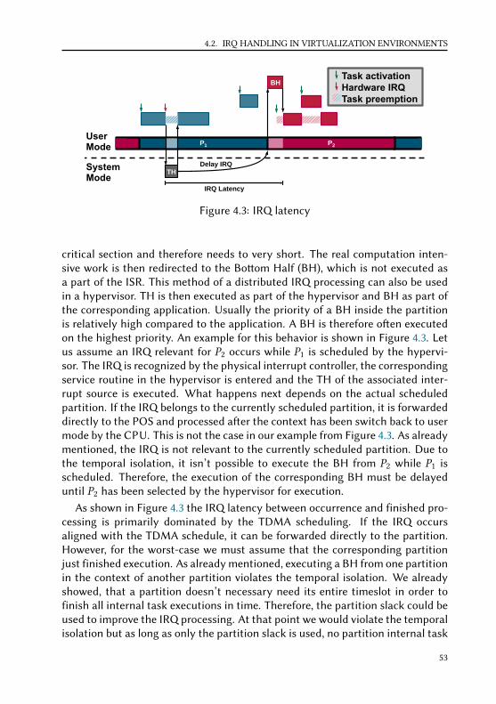
4.2. IRQ HANDLING IN VIRTUALIZATION ENVIRONMENTS
P2P1
BH Task activation Hardware IRQ Task preemption
TH
User Mode
System Mode
IRQ Latency
Delay IRQ
Figure 4.3: IRQ latency
critical section and therefore needs to very short. The real computation inten-sive work is then redirected to the Boom Half (BH), which is not executed asa part of the ISR. This method of a distributed IRQ processing can also be usedin a hypervisor. TH is then executed as part of the hypervisor and BH as part ofthe corresponding application. Usually the priority of a BH inside the partitionis relatively high compared to the application. A BH is therefore oen executedon the highest priority. An example for this behavior is shown in Figure 4.3. Letus assume an IRQ relevant for P2 occurs while P1 is scheduled by the hypervi-sor. The IRQ is recognized by the physical interrupt controller, the correspondingservice routine in the hypervisor is entered and the TH of the associated inter-rupt source is executed. What happens next depends on the actual scheduledpartition. If the IRQ belongs to the currently scheduled partition, it is forwardeddirectly to the POS and processed aer the context has been switch back to usermode by the CPU. This is not the case in our example from Figure 4.3. As alreadymentioned, the IRQ is not relevant to the currently scheduled partition. Due tothe temporal isolation, it isn’t possible to execute the BH from P2 while P1 isscheduled. Therefore, the execution of the corresponding BH must be delayeduntil P2 has been selected by the hypervisor for execution.
As shown in Figure 4.3 the IRQ latency between occurrence and finished pro-cessing is primarily dominated by the TDMA scheduling. If the IRQ occursaligned with the TDMA schedule, it can be forwarded directly to the partition.However, for the worst-case we must assume that the corresponding partitionjust finished execution. As already mentioned, executing a BH from one partitionin the context of another partition violates the temporal isolation. We alreadyshowed, that a partition doesn’t necessary need its entire timeslot in order tofinish all internal task executions in time. Therefore, the partition slack could beused to improve the IRQ processing. At that point we would violate the temporalisolation but as long as only the partition slack is used, no partition internal task
53

CHAPTER 4. ARINC653 BASED HYPERVISOR SCHEDULING
would miss its deadline. With other words this means, that the behavior of othertasks or IRQs may interfere with another task but only to a certain degree. Thisleads us to the definition of the suicient temporal isolation bound.
Definition 4.3: Suicient temporal isolation bound
A scheduler Si provides a suicient temporal isolation bound to a task τj onϕi if
I Sij (∆t) = f I (∆t, Γi ,Si ) ≤ I Sij (∆t) (4.8)
bSij (∆t) = fb (∆t, Γi ,Si ) ≥ bSij (∆t) (4.9)
where both the received interference I Sij (∆t) and the received service bSij (∆t)on ϕi only depend on the size of the considered time window ∆t , the usedscheduler Si and the corresponding task-set Γi . The behavior of any othertask τk ∈ Γi \τj onϕi may aect I Sij (∆t) or bSij (∆t), but the impact on both
is limited to the behavior of a scheduler Si which would provide temporalisolation to the same task-set. Both, received interference and received serviceonly need to satisfy (4.8) or (4.9) as long as τj is not idle.
Therefore, as long as the caused interference is never higher or the receivedservice is never lower compared to temporal isolation for a task with outstandingworkload, the suicient temporal isolation bound is valid.
4.3 Monitoring based IRQ shaping in partitioned virtual-ization environments
The fast processing of IRQs is a well-known topic in standard OSs or small Real-Time OSs (RTOSs). Nevertheless, the latencies in virtualization environmentshave only received limited aention in the literature so far. Most of the workdone so far addressed only latencies with the hypervisor, not including the BHin the application.
As an example, [91] examined credit-based scheduler of the Xen hypervisorwith its shortcoming for IRQ latencies. The credit-based scheduler boosts par-titions (called domains) to a higher scheduling priority if they receive an IRQ.While this shortens the response times for IRQs it doesn’t ensure temporal iso-lation, as the partitions are immediately boosted even if it causes a deadlinemiss in another partition. Even the fact that the partitions were only boostedfor one short time slice in order to respond on the IRQ, a number of IRQs largeenough still violates temporal isolation. This approach was later refined in [72]
54
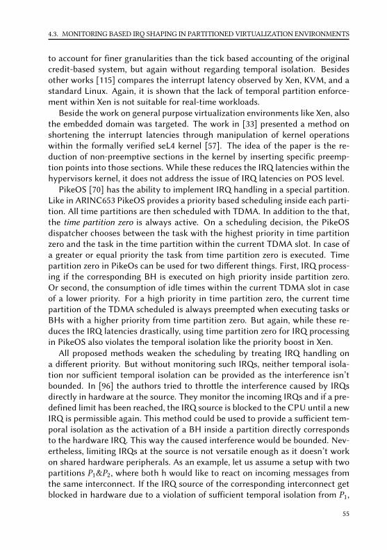
4.3. MONITORING BASED IRQ SHAPING IN PARTITIONED VIRTUALIZATION ENVIRONMENTS
to account for finer granularities than the tick based accounting of the originalcredit-based system, but again without regarding temporal isolation. Besidesother works [115] compares the interrupt latency observed by Xen, KVM, and astandard Linux. Again, it is shown that the lack of temporal partition enforce-ment within Xen is not suitable for real-time workloads.
Beside the work on general purpose virtualization environments like Xen, alsothe embedded domain was targeted. The work in [33] presented a method onshortening the interrupt latencies through manipulation of kernel operationswithin the formally verified seL4 kernel [57]. The idea of the paper is the re-duction of non-preemptive sections in the kernel by inserting specific preemp-tion points into those sections. While these reduces the IRQ latencies within thehypervisors kernel, it does not address the issue of IRQ latencies on POS level.
PikeOS [70] has the ability to implement IRQ handling in a special partition.Like in ARINC653 PikeOS provides a priority based scheduling inside each parti-tion. All time partitions are then scheduled with TDMA. In addition to the that,the time partition zero is always active. On a scheduling decision, the PikeOSdispatcher chooses between the task with the highest priority in time partitionzero and the task in the time partition within the current TDMA slot. In case ofa greater or equal priority the task from time partition zero is executed. Timepartition zero in PikeOs can be used for two dierent things. First, IRQ process-ing if the corresponding BH is executed on high priority inside partition zero.Or second, the consumption of idle times within the current TDMA slot in caseof a lower priority. For a high priority in time partition zero, the current timepartition of the TDMA scheduled is always preempted when executing tasks orBHs with a higher priority from time partition zero. But again, while these re-duces the IRQ latencies drastically, using time partition zero for IRQ processingin PikeOS also violates the temporal isolation like the priority boost in Xen.
All proposed methods weaken the scheduling by treating IRQ handling ona dierent priority. But without monitoring such IRQs, neither temporal isola-tion nor suicient temporal isolation can be provided as the interference isn’tbounded. In [96] the authors tried to throle the interference caused by IRQsdirectly in hardware at the source. They monitor the incoming IRQs and if a pre-defined limit has been reached, the IRQ source is blocked to the CPU until a newIRQ is permissible again. This method could be used to provide a suicient tem-poral isolation as the activation of a BH inside a partition directly correspondsto the hardware IRQ. This way the caused interference would be bounded. Nev-ertheless, limiting IRQs at the source is not versatile enough as it doesn’t workon shared hardware peripherals. As an example, let us assume a setup with twopartitions P1&P2, where both h would like to react on incoming messages fromthe same interconnect. If the IRQ source of the corresponding interconnect getblocked in hardware due to a violation of suicient temporal isolation from P1,
55

CHAPTER 4. ARINC653 BASED HYPERVISOR SCHEDULING
IRQ for activepartition?
Forward IRQ
Hardwarespecific
Return fromIRQ
Yes No
Dir
ect
Del
ayed
(a) Without monitoring
IRQ for activepartition?
Forward IRQ
Hardwarespecific
Return fromIRQ
Monitor satisfied?
Switchpartition
Yes
Yes
No
No
Dir
ect
Del
ayed
Inte
rpo
sed
(b) With monitoring
Figure 4.4: basic IRQ handling inside the hypervisor
also all relevant IRQs for P2 would be blocked.In order to provide an improved IRQ handling we propose an IRQ shaping,
based on the monitoring introduced by [87]. The general idea is to switch tem-porary the partition context in order to execute the BH and preserving a suicienttemporal isolation through the monitor. For a versatile behavior the monitoringis implemented as part of the IRQ handling inside the hypervisor. Figure 4.4compares both the handling without (Figure 4.4a) and with (Figure 4.4b) moni-toring. First of all, in both cases the hardware specific IRQ handling is executed.This might include reading registers as well as reseing flags. Second the IRQis forwarded to the partition-level. How this is performed depends on the usedhypervisor and POS. As an example, the evaluation setup from Chapter 8 withµC/OS-MMU as hypervisor and µC/OS-II as POS uses soware queues for BHprocessing. Therefore, in case of µC/OS-MMU and µC/OS-II the IRQ wouldbe pushed to a partition specific queue. Without monitoring, the hypervisor re-turns from the IRQ and executes the previously partition. Solely for evaluationpurpose we label the IRQs according the occurrence over time. If an IRQ belongsto the previously preempted partition, it is labeled as Direct. If the correspond-ing partition isn’t scheduled when the IRQ occurs, it is labeled as Delayed, whichwould be the case for the example from Figure 4.3.
56
4.3. MONITORING BASED IRQ SHAPING IN PARTITIONED VIRTUALIZATION ENVIRONMENTS
P2P1
BH
Task activation Hardware IRQ Monitoring Context switch Task preemption
TH
User Mode
System Mode
IRQ Latency
P2 P1
Figure 4.5: IRQ latency with shaping
Adding a monitoring as shown in Figure 4.4b only aects the handling fornon-Direct IRQs. Instead of delaying the IRQ directly, a monitoring algorithmchecks if an interposed execution of the BH would violate the suicient tempo-ral isolation of the preempted partition. If an execution is allowed, the storedpartitions context is changed so that when the hypervisor returns from IRQ topartition context, the partition of the corresponding BH is executed. This ad-ditional case is labeled as Interposed in Figure 4.4b. The resulting behavior forthe partition schedule from Figure 4.3 is presented in Figure 4.5. Aer handlingthe hardware specific stu and forwarding the IRQ to P2, the monitoring mech-anism is entered. The monitoring mechanism from [87] uses minimum distancefunctions as bounds for incoming events (or IRQs) and performs with a constantruntime overhead. Next, the context is switched to P2 and the corresponding BHis executed. In order to ensure a suicient temporal isolation the execution of theinterposed BH needs to be accounted, such that only the unused partition slackof P1 (or any other partition than P2) is used. Therefore, the hypervisor switchesautomatically to P1 aer a defined time (usually the WCET of the correspondingBH). Alternatively, P2 should also be able to switch back on its own through asystem call if the BH finishes earlier.
The amount of time that can be used to serve BHs from other partitions islimited to the partition slack, as this time is not necessary needed to finish allpartition internal task activations in time. The monitoring from [87] can be im-plemented with a constant runtime and memory overhead. In general, it workson the same minimum distance functions as used for the multiple event busy-window. Therefore, δ−(q) returns the minimum distance between the first andthe q′th consecutive event. Using this as a monitoring constraint means, thatthe last q events must be at least be separated by the according minimum dis-tance. The authors in [87] proved, that for a certain group of distance functions
57

CHAPTER 4. ARINC653 BASED HYPERVISOR SCHEDULING
Listing 4.1: Simple minimum distance monitoring
1 #define Yes 12 #define No 03 unsigned int monitor_satisfied(mon_t *mon , unsigned int timestamp)4 5 unsigned int q = 2;6 unsigned int result = Yes;7 mon ->add_to_tb(timestamp ); /* Add current event to tracebuffer (tb). */8 for (q = 2; q <= mon ->l; q++) /* Check if the last l events satisfy the */9 /* minimum distance function. */
10 if(d_in_tb(mon ,q) < min_d(mon ,q)) /* Set "return" to NO if an event violates */11 result = No; /* the minimum distance. */12 13 14 return result;15
it is suicient to only check the last l events, which limits the buer needed forthe monitoring. An example implementation for such a monitoring is shown inListing 4.1. The function monitor_satisfied() gets a monitor handle (mon) and thetimestamp of the current event (IRQ in our case) as parameter. Return value ofthe function is either 1 or 0, representing “Yes” or “No” from Figure 4.4b. First, thetimestamp of the current event is added to the tracebuer of the correspondingmonitor. Next, for the last l events the temporal distance inside the tracebueris checked against the defined minimum distance function of the monitor. Iffor one of the checked distances the defined minimum distance is larger thanthe actual observed distance, the function returns “No”. Otherwise, the functionreturns “Yes” and the BH can be interposed.
Both, runtime and memory overhead of Listing 4.1 depend directly on thetrace length (mon->l). From the available partition slackTp,S and the worst caseexecution time of the interposed BH, we can derive the needed trace length aswell as the minimum distance function. Let us assume that the BH itself has anWCET of CBH . Additionally, the needed time for context switching (CCtx ) andmonitoring (CMon ) needs to be accounted. The allowed number np of interposedBHs according to the behavior from Figure 4.5 is then given as:
np =
⌊Tp,S
CBH +CMon + 2 ·CCtx
⌋(4.10)
At this point it is important, that CMon itself depend on np as the loop in List-ing 4.1 is executed np -times. This can be neglected if CBH + 2 · CCtx >> CMon ,otherwise we need to modify the previous equation. First we substitute with
CA = CBH + 2 ·CCtx , CMon = CB · np
where CB is the WCET of one monitoring loop iteration. With this we get
58
4.4. WCRT ANALYSIS
np =Tp,S
CA + np ·CB
np · (CA + np ·CB ) = Tp,S
np2 + np ·
CA
CB−Tp,S
CB= 0
which can be solved with the PQ-equation to:
np = −CA
2 ·CB±
√√√[CA
2 ·CB
]2
+Tp,S
CB
As all times are positive we can ignore the negative solution. Also, we need toapply the floor function as we can’t handle half BHs. This leads us to
np =
−CA
2 ·CB+
√√√[CA
2 ·CB
]2
+Tp,S
CB
(4.11)
representing a more accurate solution for the number of allowed BHs.The monitoring must enforce that within a time cycle of TTDMA length only
np events are allowed. On the other hand this means that the np + 1 event needsto be at least TTDMA time units separated. This leads to a monitoring length oflp = np+1. The corresponding minimum distance function δ−BH ,p (q) is then givenas:
δ−BH ,p (q) =
0, q ≤ np
TTDMA, q > npq ∈ [2 . . .np + 1] (4.12)
With (4.10) and (4.12), a monitor can be configured in order to enforce suf-ficient temporal isolation. Nevertheless, a formal description for IRQ responsetimes is still missing. Also, we still don’t know how the partition slack, availablefor interposed BH processing, can be determined. For this reason, the followingtwo sections will deal with exact those topics.
4.4 WCRT analysis
For the response time analysis, we will provide dierent definitions for the block-ing term Bp,i (∆t) from (4.3). The dierent blocking terms will be named accord-ing to their scheduling techniques. With BTSPPp,i (∆t) we provide a first block-
59

CHAPTER 4. ARINC653 BASED HYPERVISOR SCHEDULING
ing term for a partition-level TDMA BTDMAp (∆t) and task-level SPP BSPPp,i (∆t)
scheduling.
BTSPPp,i (∆t) = BTDMAp (∆t) + BSPPp,i (∆t) (4.13)
In order to include also the interference caused by IRQs, we need an additionalBI RQ (∆t). This leads to a Bp,i (∆t) given as
Bp,i (∆t) = BI RQ (∆t) + BTSPPp,i (∆t) (4.14)
where BI RQ (∆t) includes the blocking caused by each TH. In general, an IRQcan be described as a task on a high priority. BI RQ (∆t) includes the interferenceof all THs executed in system (or even hypervisor) mode of the underlying CPU.Therefore, BI RQ (∆t) can be wrien as
BI RQ (∆t)∑
j ∈ΓI RQ
η+j (∆t) ·C j (4.15)
where ΓI RQ includes all available IRQ sources and C j describes the worst-caseexecution time of the corresponding TH. The activation paern is abstracted viaη+j . Possible activation paern in the automotive domain for IRQs range from asporadic or periodic bursts to a purely sporadic or periodic behavior.
As already discussed, the IRQ handling is divided into two parts. We alreadycharacterized the TH as a task within the context of the hypervisor, same canbe done within the partition context for each BH. Therefore, the dierent BHsinside a partition can be described as a simple task with an execution time Cp,iand a priority higher than the application related task. The activation paern ofa BH is the same as the corresponding TH executed in the hypervisor context.This leads us to
BSPPp,i (∆t) =∑
j ∈hp(τp ,i )
η+p, j (∆t) ·Cp, j (4.16)
where hp(τp,i ) is the set of tasks inside partition p with a higher or equal prior-ity as the considered task τp,i . This includes also all BHs inside the consideredpartitions.
As mentioned in Section 3.2 the busy-window based RTA was initially de-signed for work-conserving schedulers. TDMA at this point is not work-conservingas shown in Section 4.1 and Figure 4.1. A simple way to deal with this is, to de-scribe all other time partitions as interfering tasks. The execution time of theinterfering time partition is equal to their timeslot sizes. This leads to
60

4.4. WCRT ANALYSIS
BTDMAp (∆t) =
∑j ∈(ΓHYP \p)
η+j (∆t) ·Tj
where η+j (∆t) describes a periodic activation every TTDMA time units for eachtime partition. Replacing the activation paern with the actual periodic activa-tion gives us
BTDMAp (∆t) =
∑j ∈(ΓHYP \p)
⌈∆t
TTDMA
⌉·Tj
where d∆t/TTDMAe could also be placed outside the sum. Considering (4.1) wecan also rewrite the sum. As a result, the TDMA based blocking BTDMA
p (∆t)can be constructed only based on the corresponding slot size Tp and the overallTDMA cycle length TTDMA.
BTDMAp (∆t) = (TTDMA −Tp ) ·
⌈∆t
TTDMA
⌉(4.17)
When considering response times for IRQs, a RTA of the corresponding BHprovides the desired result. Due to the additional interference from all THs inBI RQ (∆t), the time needed for execution of the corresponding TH is directly in theconsidered interference. This is possible, as the execution of both, TH and BH candirectly be used for the corresponding interference or task execution time. Withthe introduction of the monitoring based IRQ shaping, we need to modify thisvalues, as additional soware overhead for monitoring and context switchingis introduced. Figure 4.4b and Figure 4.5 show the dierence of executing aninterposed or direct IRQ. In case of a direct IRQ, no monitoring inside TH and alsono context switch for the corresponding BH is needed. Compared to Figure 4.4a,an implementation of Figure 4.4b must check the active partition, as the handlingfor a foreign partition is dierent. For a direct handled IRQ only an additionalif-statement would be checked which could be neglected execution time wise.Nevertheless, the worst-case interference by IRQ handling is generated for aninterposed IRQ. As a result we need to change the WCET values for both, THand BH. The primary overhead introduced to the TH is due to the monitoring.Therefore, we get a modified TH WCET for IRQ source j, which can be used in(4.15).
C j = C j ,TH +CMon (4.18)
In case of an interposed BH, the additional overhead is based on the introducedcontext switches. Finally, we get a modified BH WCET for IRQ source j insidepartition p, which can be used in (4.16).
61
CHAPTER 4. ARINC653 BASED HYPERVISOR SCHEDULING
Cp, j = Cp, j ,BH + 2 ·CCtx (4.19)
With (4.18) and (4.19) the response times can be calculated based on (4.14).Under consideration that all IRQs adhere to the monitoring and the availableslack, BTDMA
p (∆t) could be removed from BTSPPp,i (∆t), leading to the desired be-havior from Figure 4.5.
4.5 Time Cycle Optimization
The described IRQ shaping from Section 4.3 shows how to improve IRQ responsetimes due to the use of partition slack. Nevertheless, Section 4.3 does not con-sider the design of a partition setup which can benefit from this method. Withinthe context of ARINC653, several approaches for time partition calculation areavailable. One of the most frequently mentioned works within this context is[76]. The authors of [76] provided an overview of the APEX interface and intro-duced a method to optimize the time partitions with RMS inside. This methodcan now be used for the described analysis in Section 4.4, as IRQs can rarely bedescribed by RMS. Another optimization method for time partitions was pro-vided in [111]. They used a meta-heuristic approach called simulated annealingto optimize time partitions. Nevertheless, the used system model does not con-sider a scheduling on partition-level. To solve this issue, we show in this sectionhow a partition setup with maximized partition slack can be generated. As theoptimization algorithm is based on the analysis introduced in Chapter 3 and ex-tended in section 4.1/4.4, it is able to handle arbitrary IRQ/task activation paernas well as arbitrary deadlines.
4.5.1 Optimization algorithm
Figure 4.6 shows the proposed optimization algorithm. General idea of the algo-rithm is to calculate a minimum timeslot sizeTp,min for each of the Ω partitionsand a given TTDMA. From those values the slack in the entire TDMA cycle canbe derived and distributed to the dierent partitions. For the optimization al-gorithm it is necessary to calculate an upper bound for the TDMA cycle lengthTTDMA. The upper bound TTDMA is used as starting condition for the optimiza-tion algorithm. We will first show the concept of the algorithm and provide aformal proof for the starting condition aerwards in Section 4.5.2.
The algorithm starts on the upper le corner with assigning the upper boundTTDMA to TTDMA. Next the partition analysis is started, which returns a tupleof minimum partition sizes (T1,min, . . . ,TΩ,min) for the current TTDMA. The cal-culation of the Tp,min values is shown on the right side of Figure 4.6 and will be
62

4.5. TIME CYCLE OPTIMIZATION
PartitionAnalysis
Done
Saveconfiguration
Yes
No
No TS≥0
TTDMA≤Δ
Pick bestconfiguration
Yes
TTDMA=TTDMA
No
TTDMA=TTDMA−Δ
p=1
Tp,min=Δ
Foreach τp , i∈ΓpRp , i≤Dp , i
PerformRTAForeach τp , i∈Γp
Tp, min=Tp ,min+Δ
Yes
p=λ
Return
p=p+1
No
Yes
Partition Analysis
Figure 4.6: Laxity based upper bound for TTDMA
explained later. The partition analysis calculates for each partition the smallesttime partition, so that it reaches all deadlines at the considered TTDMA. As weknow from (4.1), the sum of all time partitions must beTTDMA. At this point it ispossible that the sum over all calculated minimum time partition sizes is smaller,equal or larger thanTTDMA. Therefore, we introduce the TDMA cycle slackTS asdierence between considered TTDMA and minimum time partition sizes.
TS = TTDMA −
Ω∑p=1
Tp,min (4.20)
According to the sum over the minimum time partition sizes, TS can be smaller,equal or larger than zero:
63

CHAPTER 4. ARINC653 BASED HYPERVISOR SCHEDULING
TS < 0: If the time cylce slack is negative, the sum of the required mini-mum time partition sizes is larger than TTDMA. This means, thatthe time partitions need more execution time than actual avail-able. The partition setup is not schedulable for the consideredTTDMA.
TS = 0: If the time cylce slack is zero, the needed minimum executiontime by the time partitions is equal to the available time during aTDMA cycle of size TTDMA. This means, that the partition setupis schedulable for the considered TTDMA, but it does not provideany slack for additional IRQ handling.
TS > 0: If the time cylce slack is positive, the needed minimum executiontime by the time partitions is smaller than the available time dur-ing a TDMA cycle of size TTDMA. This means, that the partitionsetup is schedulable for the considered TTDMA and the availableslack can be used for additional IRQ handling.
The target of the optimization algorithm is to find all possible time cycle config-urations which provide a schedulable system. Therefore, only time cycle config-urations with TS ≥ 0 are saved for later use in Figure 4.6.
Next, the current TTDMA is checked against a step size ∆. If TTDMA ≤ ∆,the calculation of possible time cycle configurations is stopped. Otherwise, theTTDMA is decreased by ∆ and the partition analysis is restarted for the newTTDMA. The granularity of ∆ directly influences the optimization algorithm. Asmaller ∆ increases both, runtime and accuracy of the optimization algorithm.While a bound on the granularity is usually independent of the executed so-ware, the underlying hardware instead provides a lower bound for ∆, as theTDMA schedule needs to be generated or controlled by a hardware timer. The ∆can therefore directly be derived by the granularity of the hardware timer usedof schedule generation. Choosing a finer granularity than the hardware can pro-vide only increases the algorithm runtime, but does not improve the accuracy.Aer the partition analysis has been performed for the last TTDMA, the best so-lution is picked and the available time cycle slack is distributed to the partitions.A beer explanation of this process will be given later in Section 4.5.3.
Aer knowing the outer layer of the optimization algorithm, we can now focuson the partition analysis on the right of Figure 4.6 which calculates the neededminimum time partition sizes for a given TTDMA. The analysis starts with thefirst partition and assigns ∆ as minimum time partition size Tp,min . Next, a RTAbased on (4.14) is performed. Aerwards the schedulability is checked accordingto Definition 3.16. If one of the task deadlines in the corresponding partition ismissed, Tp,min is increased by ∆ and the RTA is repeated. This is done until alltasks inside the considered partition reach their deadlines and repeated for all Ω
64

4.5. TIME CYCLE OPTIMIZATION
... PλP1
Task activation
P1
ε ε
D1,i
L1,i
C1,i
TTDMA
TTDMA -T1
Figure 4.7: Laxity based upper bound for TTDMA
partitions. Due the fact, that (4.14) only depends on partition internal parametersand the given TTDMA, the inner loop of the partition analysis can be executedin parallel. As a result the partition analysis returns a tuple of minimum timepartition sizes which represent the minimum time each partition needs for thegiven TTDMA.
4.5.2 Laxity based time cycle bound
The optimization algorithm simply searches for possible time cycle configura-tions in a given interval. While the lower bound is provided by the step sizegranularity, the upper bound is given as TTDMA. The information included inTTDMA is that the considered system is impossible to schedule for a cycle lengthTTDMA > TTDMA. Therefore, TTDMA provides an upper bound, which can be usedby the algorithm in Figure 4.6.
Lemma 4.1: Upper bound for TDMA cycle length
A suicient upper bound TTDMA, without considering additional task activa-tions for higher prior tasks within the same partition is given through:
TTDMA =
∑Ωp=1 min
τp ,i ∈ΓpDp,i −Cp,i
Ω − 1(4.21)
The proof of this theorem can be derived based on Figure 4.7. Let us assumethat a task τ1,i in P1 is activated such that it is impossible to finish the executionduring the current TDMA cycle. Resulting from this, a small amount time (ϵ) isneeded to finish the execution within the following cycle as shown in Figure 4.7.For the execution of τ1,i we assume that no interference is caused by other tasksfrom P1. As a result we can see in Figure 4.7, that the maximum amount of time
65

CHAPTER 4. ARINC653 BASED HYPERVISOR SCHEDULING
τ1,i can be preempted by the TDMA schedule without missing its deadline islimited to the laxity of the considered task.
L1,i = D1,i −C1,i ≥ TTDMA −T1 (4.22)
If we would consider the activation paerns and include partition internal block-ing, the maximum TDMA cycle length would be decrease as the maximum al-lowed interference is still limited by the laxity. While (4.22) is only valid for theconsidered task in the example from Figure 4.7, we need to generalize this ap-proach for an entire task-set inside a partition. A suicient bound is provided ifwe use the task with the minimum laxity inside a partition p. This leads us to
Lp = minτp ,i ∈Γp
Dp,i −Cp,i (4.23)
where we consider Lp as the minimum partition laxity of partition p. Combining(4.22) and (4.23) leads us to.
Lp = minτp ,i ∈Γp
Dp,i −Cp,i ≥ TTDMA −Tp =Ω∑i=1
Ti −Tp (4.24)
When considering the maximum allowed blocking time, the minimum partitionlaxity is equal to the interference caused by a TDMA cycle with length TTDMA.
Lp = TTDMA −Tp =Ω∑i=1
Ti −Tp (4.25)
If we evaluate this for all Ω partitions, we can describe it as a system of linearequations for beer illustration.
AΩ,Ω =
0 1 . . . 1 11 0 . . . 1 1...
...1 1 . . . 1 0
, ®t =
T1T2...TΩ
, ®l =
L1L2...LΩ
AΩ,Ω ·
®t =®l
The multiplication AΩ,Ω ·®t gives us:
0 +T2 + . . . +TΩ−1 +TΩT1 + 0 + . . . +TΩ−1 +TΩ
...T1 +T2 + . . . +TΩ−1 + 0
=
L1L2...LΩ
(4.26)
66

4.5. TIME CYCLE OPTIMIZATION
Now we are close to finish. If we take a closer look on the le side of the equation(4.26), we can see that in each row one time partition is missing. As an example,due to (4.23)T1 is missing for L1,T2 is missing for L2 and so on. This means, thateach time partition is included (Ω − 1) times in the listed Ω rows. Calculatingthe sum over the Ω rows leads to:
(Ω − 1) · (T1 +T2 + . . . +TΩ) =Ω∑p=1
Lp
Replacing the sum of time partitions with TTDMA and Lp with (4.23) finalizes theproof of Lemma 4.1.
(Ω − 1) · TTDMA =
Ω∑p=1
minτp ,i ∈Γp
Dp,i −Cp,i
TTDMA =
∑Ωp=1 min
τp ,i ∈ΓpDp,i −Cp,i
(Ω − 1)(4.27)
4.5.3 Slack distribution
The previous two sections explained how the time cycle configurations with addi-tional slack can be calculated. Nevertheless, we neither explained in Section 4.5.1how to pick one of the possible solutions nor how the calculated slack is assignedto dierent partitions. The reason for this is that the strategies for both tasks maydepend on the actual implemented applications. Figure 4.8 shows the availableslack over all checked TDMA cycles. The shown values in Figure 4.8 have beengenerated for a partition setup which will be explained and used later duringevaluation in Section 8.1.2. All times labeled on the axis are given in millisec-onds.
Figure 4.8a shows the absolute time cycle slack over the entire algorithm work-space from TTDMA down to ∆. Which of the possible configurations is “the bestsolution” can’t be said directly. As we can see, a global maximum for TS is givenfor a setup with ∼ 48ms . At first glance one might think, that the absolute max-imum slack always provides the best partition configuration, but this doesn’tneed to be the case. The time cycle slack is available each TTDMA time units,therefore it is possible that a configuration with less slack during a time cycleprovides more slack within a larger time window. In order to visualize this, Fig-ure 4.8b shows the available slack normalized to the corresponding TTDMA. Bycoincidence for the used example, the global maximum at ∼ 48ms is still a maxi-
67

CHAPTER 4. ARINC653 BASED HYPERVISOR SCHEDULING
TTDMA
TTDMA
Δ
TS
max TS
Algorithm workspace
0102030405060708090
-20
-15
-10
-5
0
5
10
15
20
(a) Absolute
TTDMA
TTDMA
Δ
TS/TTDMA
Algorithm workspace
0102030405060708090
-0,4
-0,3
-0,2
-0,1
0
0,1
0,2
0,3
0,4
(b) Normalized
Figure 4.8: Available slack within algorithm workspace
mum even if it is normalized to the corresponding time cycle. Nevertheless, sev-eral other configurations provide the same amount of normalized slack. At thispoint it depends on the actual applications inside, which of the possible config-urations fits the needs best. A longer time cycle reduce the number of contextswitches, which is oen a desirable goal. Especially when using a method like thedescribed IRQ shaping which introduces additionally context switches. Also, alonger time cycle and therefore longer partitions may also shorten the responsetimes of the internal tasks as those may finish within one time cycle. On theother hand, if a task doesn’t finish its execution within one time partition, thedelay caused by the TDMA scheduling is large. Once a configuration has beenpicked for usage, the available time cycle slack needs to be distributed to thedierent time partitions. The distribution of the time cycle slack to the dierentpartitions also heavily depends on the actual applications inside the partitions. Ifone partition implements more IRQ handling on partition-level it benefits most,if the slack is primarily distributed to the other partitions. Also, if the IRQs followa specific event model (like periodic bursts), the slack distribution across the par-tition could be aligned to this event model. If none of the previous preconditions
68

4.6. FORMAL LIMITATIONS OF IRQ SHAPING
are given, an equal slack distribution to the partitions could be desirable.
Tp,S = TS ·
⌊Tp,min∑Ωi=1Ti ,min
⌋(4.28)
In this case the time cycle slack is distributed to the dierent partitions based ontheir minimum time partition sizes. Based on Definition 4.1 and (4.28) the finaltime partition sizes can be calculated. As described in Section 4.3, the monitoringis then configured according to the dierent Tp,S values.
Both, the selection of the “best” configuration and the “best” slack distribu-tion heavily depend on the actual applications inside the partitions. As discussedan optimization for both depend on more than one factor, therefore we do notpinpoint one method as “the best solution”. Without any knowledge about appli-cations and/or IRQ paern an equal distribution of the available slack based ona configuration with maximum slack per time cycle is a step towards the rightdirection. If several configurations provide the same amount of slack per timecycle, the configuration for the largest TTDMA is desirable in order to minimizecontext switching.
4.6 Formal limitations of IRQ shaping
The monitoring based IRQ shaping provides a simple relaxation of the strictTDMA scheduling. When considering Section 4.3 and Section 4.4, we can clearlysee that the IRQ processing is improved drastically for IRQs handled throughthe monitoring based shaping. This way the average response time for IRQs isreduced and the scheduling is improved, as certain idle times during schedulingcan be used for IRQ processing. Nevertheless, the proposed method has certaindisadvantages.
First of all, the IRQ shaping only improves the WCRT of IRQs, if all possibleIRQs always occur during the time partition of the correct partition or when slacktime is available. If this is not given due to insuicient slack or unknown behaviorof IRQs, only the average response time is improved but not the WCRT. Second,the monitoring from [87] is not ideal for such an enforcement of temporal isola-tion as it does not scale ideally. As shown in Listing 4.1 both memory usage fortrace buer and the runtime overhead scale linear with number of events needto be checked. The calculation of the number of allowed events (or in our caseIRQs) is given through (4.10) (or (4.11)). This shows directly that the monitoringfor a system with a lot of slack generates more overhead than for a system withless slack. While more slack is available in theory, it can’t be used as eicientas possible due to additional overhead. Third, even though we consider IRQsas tasks during the analysis, we still limit the usage of slack to IRQs. Indirectly
69

CHAPTER 4. ARINC653 BASED HYPERVISOR SCHEDULING
P2P1
BH Task activation Hardware IRQ Task preemption
TH
User Mode
System Mode
P2 P1
TH
BH
Delay
Delay
Figure 4.9: Limitation of IRQ shaping
this means, that a normal task can not use the available slack when it’s activa-tion occurs within a foreign time partitions. This leads us the fourth and worstdisadvantage. The scheduling is still not work conserving.
Even for IRQs this is not the case as shown in Figure 4.9. Let us assume thatthe slack of P1 allows the execution of one foreign BH within its time partition.As discussed, the slack calculation is based on the busy-window method whichtakes the critical instant as starting condition. It is therefore possible, that thisworst-case behavior of simultaneous task activations is not always the case. Thecritical instant might include another task in P1 which needs to be finished butisn’t executed in each time cycle. As a result P1 would be idle during this and asthe calculated slack is based on the critical instant, no BH could be interposed.This is shown in Figure 4.9. First a BH is interposed during P1. As a result theavailable slack T1,S is consumed and the currently executed task in P1 is pre-empted. Second, the preempted task resumes and finishes its execution. At thispoint P1 is idle, but since the time partition slack was already consumed, thefollowing BH or task activations for P2 must be delayed in order to satisfy thesuicient temporal isolation. Reason for this behavior is the fact, that the moni-toring based shaping does not consider if the currently executing partition whichshould be preempted is idle or not. As a result, the monitoring doesn’t know thatinterposing the BH a second time would not cause any deadline misses. In or-der to enable such a behavior we show in the following chapter how to modifyan SPS based budget scheduling. Main objective is to provide a replacement ofthe previously described TDMA based scheduling, which takes account of eachpartitions actual required workload.
70

CHAPTER5
Sporadic Server based Budget Scheduling
“I’m sciencing as fast as I can!”
- Professor Hubert J. Farnsworth
As discussed in Chapter 4, the TDMA based scheduling is less optimal for systemswith sporadic events like IRQs. In order to react on such events suiciently amore flexible scheduling, which still preserves a suicient temporal isolation, isneeded. This chapter shows how the existing SPS mechanism can be modifiedin order to replace a TDMA based scheduling as used in ARINC653. Most of thework used in this chapter was previously presented in [26] and [24].
The SPS was first proposed in [108] and has become a part of POSIX [113] asa scheduling policy. The general idea was to provide a performant schedulingmechanism with temporal isolation for aperiodic (sporadic) task activation. Foreach aperiodic task, the SPS defines an execution budget and a replenishmenttime. In contrast to other mechanisms like the deferrable server mentioned in[108] or the priority exchange server, the SPS does only replenish an executionbudget if it was used before.
The basic functionality of the SPS mechanisms can be explained best with anexample, like shown in Figure 5.1. Each task τi has an execution time budgetbi , which is initialized to its maximum value bi ,max at the beginning. Whena task τi is executed, the corresponding budget bi is decreased. A downwardsslope in Figure 5.1 therefore indicates a time range, where the correspondingtask is picked by the scheduler for execution. Due to the specification of the SPS
71

CHAPTER 5. SPORADIC SERVER BASED BUDGET SCHEDULING
t0t1 t2 t3 t4
t
Budget b1
Budget b2
Δt = TR
b1 =
b1 +
(t 1-t
0)
t0+TR t1+TR t2+TR t3+TR
b2 =
b2 +
(t 2-t
1)
b1 =
b1 +
(t 3-t
2)
b2 =
b2 +
(t 4-t
3)
b1,max
b2,max
ε ε 0
Figure 5.1: Laxity based upper bound for TTDMA
algorithm from [108], each task τi has a replenishment period TR,i . This way,used budget is always replenished relative to the start of the consumption (e.g.execution). In Figure 5.1 τ1 starts execution at t0 and stops at t1. During this timea budget of t1− t0 time units was consumed. At this point one obvious dierenceto a simple TDMA scheduling can be recognized. An SPS enforced task doesn’thave to consume the available budget in one piece. If all outstanding workloadhas been processed, the task can self suspend its execution. As a result, nothingof the available budget is waisted.
For the sake of simplicity, both tasks in Figure 5.1 have the same replenish-ment time TR,1 = TR,2 = TR . Due to this constraint, an amount of t1 − t0 timeunits is replenished at t0 + TR and the available budget for τ1 is increased. Thesame is done for τ2 when it stops execution at t2 and so on. [108] also definespriorities for sporadic server tasks. Those priorities specify the order in whichthe tasks are scheduled. In our example from Figure 5.1, τ1 would have a higherpriority as it is scheduled first.
The later defined POSIX standard states that each sporadic server task wouldhave two priorities. One foreground priority, used as long as the task has remain-ing budget and a lower background priority, used when the budget is depleted.However, [109] already showed the pitfalls when it comes to the implementa-tion of background scheduling. The first SPS specification in the POSIX stan-dard was not entirely correct, causing budget amplification. The primary problemwas an influenced budget replenishment based the execution during backgroundscheduling. This caused an unreliable temporal isolation, since budget was re-plenished too early. Also, there have been suggestions to implement this policyinto the Linux kernel [45] to provide additional real-time capabilities and tem-
72

5.1. ISOLATION BOUND
poral isolation. The usage of an SPS for virtualization environments has alreadybeen proposed in [79, 36]. The described kernel est V uses so called VCPUswhich are scheduled on dierent physical CPUs. est V dierentiates betweentwo types of VCPUs, called Main VCPUs for applications and I/O VCPU for IRQbased events. While the SPS was only considered for Main VCPUs, it was notused for the IRQ based workload of I/O VCPUs. Also, the authors in [117] useda standard priority based sporadic server to provide so real-time guarantees.Nevertheless, the proposed method was not designed to cover hierarchical sys-tems like ARINC653.
An analysis for tasks scheduled under a SPS policy has been proposed in [102,8]. Nevertheless, the provided analysis did neither cover background schedulingnor is it applicable for a hierarchical scheduling with SPP as defined in ARINC653.In general, there was not a lot of work considering the SPS mechanism in the lastyears. A major reason for this is the tendency towards a complex implementationof an SPS based system with several servers and dierent replenishment periods.The benefit compared to other server based scheduling solutions might be mod-erate [37]. This chapter will show, that under certain constraints a modified SPScan be a valuable replacement of the strict TDMA based partition-level schedul-ing in ARINC653. The proof, that such a system can be implemented with a lowoverhead profile is later given in Chapter 7 and 8.
5.1 Isolation bound
One of the two major advantages of the SPS is its ability to provide a suicienttemporal isolation bound as required in Definition 4.3. If we consider a timewindow ∆t = TR and move it across the time line, any task τi can never executemore than bi ,max time units during this time window. The worst-case behaviorof a task τi is given, when τi uses its budget as soon as it is available. In order toexplain this further we use again Figure 5.1.
Let’s have a look at τ1 depleting its budget b1 at t3, which lays within the firstTR time units (t0 → t0 + TR ). The caused interference by τ1 within this timewindow is equal to its maximum value b1,max as the entire budget was used forexecution. Right at t0 +TR the budget of τ1 is replenished and τ1 starts executingagain. If we shi the considered time window by ϵ time units to the right, thebudget used by τ1 inside the time window is still b1,max and can never be greaterthan that. The additional interference of size ϵ between t0 + TR → t0 + TR + ϵis equal to the interference which fell out of the considered window on the le.Therefore, the budget used by τ1 inside the considered window is still the same
As already mentioned we consider the SPS under certain constraints as a re-placement for the TDMA based partition-level scheduling in ARINC653. Based
73

CHAPTER 5. SPORADIC SERVER BASED BUDGET SCHEDULING
on the SPS mechanism, within any considered time window of size TR,p a taskτp , as part of the SPSs scheduled task-set ΓHYP , uses never more budget than de-fined in bp,max . If all SPS tasks use the same replenishment period TR as shownin Figure 5.1, a single task will never see more interference than the summarizedbudgets of all other tasks in ΓHYP within a time window ∆t = TR . This leads toa worst-case interference given as:
ISPSp (∆t = TR ) =
∑j ∈ΓHYP \p
bj ,max (5.1)
When comparing this to the TDMA interference term from (4.5) one might di-rectly recognize that the SPS mechanism provides the same isolation bound thanTDMA if we interpret the time cycle length as replenishment period and timeslotsizes as maximum budgets.
p ∈ Ω (TR,p = TTDMA,bp,max = Tp ) (5.2)
Important at this point is that the SPS provides an interference bound in theterms of a suicient temporal isolation as defined in Definition 4.3 and not atemporal isolation as defined in Definition 4.2. Reason for this is the possible selfsuspend of a task scheduled by the SPS. In case of TDMA the hypervisor wouldnot leave the context of a partition if this partition is idle. Therefore, the causedinterference in case of TDMA is in any time window of size ∆t = TTDMA equalto the worst-case, even if a partition is idle. In case of the SPS mechanism this isnot the case anymore as a partition can self-suspend its execution when it wouldbe idle otherwise. The actual interference during ∆t = TR therefore depends onthe behavior of all other tasks/partitions with a TDMA-like limitation given by(5.1).
5.1.1 Scheduler setup
Due to the previous argumentation, the SPS bounds the interference according toDefinition 4.3. But in order to provide a suicient temporal isolation bound, alsothe service (execution budget) provisioning must be considered. Since we wantto replace the scheduling algorithm of ARINC653, TDMA must be considered asa lower bound for service provisioning. In general, the SPS on its own does notdecide which task or partition should be dispatched next by the scheduler. Thiswasn’t even the case for the original POSIX definition. Instead, only the budgetconsumption and therefore the caused interference to other tasks is enforced.The POSIX definition of the SPS proposes a priority based scheduling, wheretasks use two dierent priorities. One higher foreground priority used for a taskτi whilebi > 0 and a lower background priority used whileb = 0. A task/partition
74

5.1. ISOLATION BOUND
is then scheduled according to the currently set priority whenever outstandingworkload exists. Even though the SPS controls the priorities in case of the POSIXdefinition, it doesn’t take an actual scheduling decision. As a flexible foundationwe use a generic architecture, which divides the setup into two major parts. Theactual implementation of the proposed architecture will be discussed later inSection 7.1 (Figure 7.2). This section only provides a coarse grained architectureoverview, for beer understanding of the theoretical considerations.
First, there is the standard SPS mechanism which enforces the interference.And second, there is the scheduler which is in charge of determining which par-tition should be scheduled next. The main duty of the SPS in order to providean interference bound is the control of a timer module. The timer provides twodierent signals, one for budget depletion (Empty) and another one for budgetreplenishment (Refill). The Empty signal always belongs to the current scheduledpartition, the Refill signal may belong to any partition on the same resource. Inthe proposed architecture, the SPS is also in charge of dispatching (Dispatch)partitions. This means, that the SPS is able to initiate a context switch if needed.The SPS also tracks, if a partition would like to suspend its execution (Idle). Thishappens when all tasks inside a partition served their current activation and donot have any outstanding workload. Allowing a partition to stop its execution isthe second major advantage of the SPS, as it provides the ability to reduce un-necessary blocking times. Combining this with the optimization algorithm fromSection 4.5, is the logical next step. The output of the optimization algorithmfrom Section 4.5 maximizes the slack inside the partitions and should thereforeprovide a maximized benefit from this Idle-feature. An idle partition can be re-activated with the Resume signal. In general, the Resume signal is issued when atask inside a partition is activated. Such an activation can be triggered by dier-ent events like time ticks, partition-2-partition communication or any other typeof subscribed hardware IRQs.
We already mentioned, that the SPS itself doesn’t decide which partition shouldbe dispatched next. Instead, this decision is taken by the scheduler. Generalidea of the proposed architecture is, that the SPS forwards scheduling dependentevents to the scheduler. Those events trigger callback functions inside the sched-uler. The collection of events is described by the Callback API (CB API) whichis explained later in Section 7.1.2 Each scheduler callback performs a schedul-ing decision and returns the partition which should be dispatched next by theSPS. If the returned partition diers from the currently executed one, a contextswitch is initiated. In addition to the callbacks, the scheduler also haves access tothe current budget state of each partition. Which additional environment valuesare included for decision taking, depend on the implemented scheduling mech-anism. This way the entire behavior of the system and the provided service foreach partition is under control of the scheduler.
75

CHAPTER 5. SPORADIC SERVER BASED BUDGET SCHEDULING
5.1.2 Service provisioning
In Section 4.1 we already mentioned the service provisioning for TDMA. In eachtime window ∆t = TTDMA the received service of a partition is equal to thecorresponding timeslot size Tp . If we transfer this to the SPS based schedulingthis means, that a partition must always receive its maximum budget bp,maxwithin a time window of size TR . This leads us to Definition 5.1.
Definition 5.1: TDMA-like service provisioning
In order to provide a TDMA-like service, a scheduler must enforce under allcircumstances the following constraints:
1. The maximum activation delay when resuming back from idle is limitedto TR − bp,max
2. As long as a partition p is not idle, the scheduler must provide in eachtime window of size ∆t = TR the maximum budget bp,max
Budgets and replenishment period must be assigned according to (5.2).
At this point we highlight the most important dierence between an SPS basedmechanisms and TDMA. TDMA always provides service to partition, even if itisn’t actually needed as there is no outstanding workload. In case of a SPS basedmechanism this is not the case, as only used budget is accounted and replen-ished later. In general, service provisioning is only needed for partitions whichhave outstanding workload and are currently not idle. Due to the possibility for apartition to self suspend its execution when idle, a maximum initial delay needsto be considered. In case of TDMA, the delay between an IRQ or task activationand the next time the corresponding partition p achieves service is bounded toTTDMA − Tp . This delay occurs when an activation happens right at the end ofthe corresponding time partition such that it can not be processed anymore. Anexample of such a behavior has already been shown in Figure 4.2. For a SPS basedmechanism, this must be considered separately, as the self suspend introducesan additional partition state compared to TDMA. As long as a partition is notin the idle state, the activation delay is enforced through the TDMA-like serviceprovisioning. When a partition is idle and gets resumed by any kind of activa-tion, it is not necessary to schedule the partition immediately. Instead, only theactivation delay needs to be enforced, which means that the partition is delayedby a maximum of TR − bp,max . While this enables a more flexible scheduling, itmust be ensured that this can never be violated. Simultaneously to the activationdelay the service provisioning must also be ensured. As an example, if a partitionp is delayed initially for its maximum of TR − bp,max , it must receive aerwards
76

5.1. ISOLATION BOUND
t
Prio
Hig
hM
edL
ow
Med
BG
t0 t0 +TRt1 t1 +TR t1 +2TR
Part. Resume Part. Idle
Budgets: 2 5 5
ε ε
Δt=TR Δt=TR
t2
Figure 5.2: Service provisioning according to POSIX
its entire budget of bp,max without preemption if needed. Otherwise, partition pwould not receive its maximum budget bp,max within a time window of size TR .
With Definition 5.1 in mind, a new scheduler can be developed. While thischapter focuses on the general architecture and the RTA, we postpone the ac-tual scheduler according to Definition 5.1 to Chapter 7. But before we introducethe RTA, we will first test if the standard POSIX implementation with a prioritybased scheduling is able to fulfill Definition 5.1. Let us consider a setup withthree partitions with dierent priorities as shown in Figure 5.2. The priorities forbackground scheduling are arranged in the same order as the foreground pri-orities. According to the POSIX definition, the foreground priority of a task isalways higher than the background priority. For the sake of simplicity, back-ground scheduling is only used for the medium priority partition (Med/MedBG )in Figure 5.2. The three dierent partitions have maximum budgets of (2, 5, 5)according to Figure 5.2. A partition is resumed, when one of the tasks inside isactivated. The idle state is reached when all tasks inside a partition have servedall of their outstanding activations.
In order to check if the POSIX definition of the SPS satisfies Definition 5.1, ac-tivation delay and maximized service is checked for the partition with the lowestpriority (Low). Let us consider the critical instant at t0 where all partitions areresumed at the same time. Due to the higher priorities, the low priority partitionis delayed until t1. As all other partitions already depleted their budgets, the lowpriority partition can execute until TR . Even though the medium priority parti-tion has outstanding workload, it is delayed untilTR where it is scheduled basedon its background priority. This simple example shows, that the priority basedscheduler as proposed in POSIX is able to enforce the maximum activation delay,even for the critical instant.
The second constraint of Definition 5.2 requires that all partitions receive their
77

CHAPTER 5. SPORADIC SERVER BASED BUDGET SCHEDULING
maximum budget within a time window of size ∆t = TR as long as they’re notidle. We highlighted two corresponding windows in the example from Figure 5.2.The first window from t0 → TR includes the previously discussed example andsatisfies, beside the maximum activation delay, also the required service. Thesecond window from t1 + TR + ϵ → t1 + 2 · TR + ϵ shows a dierent behavior.Although the low priority partition is not idle, it does not receive its maximumbudget within the shown time window. In order to show how this is possible letus start at t1 + TR . Here the low priority partition is resumed and dispatchedimmediately as all other partitions are idle at t1 +TR . The low priority partitionexecutes until its budget is depleted at t2. As the partition still has outstandingworkload, it does not switch back to idle. At t2 also the medium priority parti-tion is resumed, immediately dispatched and starts execution until the budgetis depleted. Now the scheduler switches to background scheduling, as both par-titions have outstanding workload but no remaining budget. In our example,also the background priority MedBG is higher than LowBG (not shown in Fig-ure 5.2). Therefore, the execution of the medium priority partition is continueduntil t1 + 2 · TR . This on its own wouldn’t be a problem, as the low priority par-tition received its maximum budget during t1 + TR → t1 + 2 · TR . In order tocontinue to do so, the low priority partition must be dispatched at t1 + 2 · TR ,where also its depleted budget is replenished. But in Figure 5.2 this is not thecase, as the high priority (High) is resumed right at t1 + 2 · TR and immediatelydispatched due to its higher priority. As a result, the received budget for the lowpriority partition during t1 + TR + ϵ → t1 + 2 · TR + ϵ is lower than the cor-responding TDMA-bound. A simple measure to avoid such a behavior is, that anon-idle partition is always dispatched immediately when budget is replenished.The second constraint of Definition 5.1 would be violated otherwise. In case ofthe POSIX conform implementation, this is not possible due to the schedulingwith fixed priorities. Again, as this chapter focuses more on the formal aspects,we postpone the actual scheduler implementation to Chapter 7. Nevertheless, forthe RTA we assume that the scheduler’s behavior is according to Definition 5.1and implements the previously mentioned measure which provides immediateservice aer replenishment for certain partitions.
5.1.3 Work conserving scheduling
One of the major requirements from Section 2.3.1 is a work conserving sched-uler. We already mentioned that this is not the case for the standard TDMAbased scheduling in ARINC653. If we take a look at the previous example fromFigure 5.2, we can see that due to the background scheduling the system neverdelays unnecessarily the execution of a partition. As an example, at t0 + TRthe medium priority enters background scheduling, since it still has outstand-
78

5.2. WCRT ANALYSIS
t
Prio
Hig
hM
edL
ow
t0 t0 +TRt1 t1 +TR t1 +2TR
Part. Resume Part. Idle
Budgets: 2 5 5
No
t w
ork
co
ns
erv
ing
No
t w
ork
co
ns
erv
ing
Figure 5.3: Service provisioning according to POSIX without background schedul-ing
ing workload but its budget was depleted at t1. This mechanism leads to a workconserving scheduling, since a partition can be picked by the scheduler for dis-patching as long as it has outstanding workload, even with an empty budget.For a scheduler without the support for background scheduling this is dierentas shown in Figure 5.3. While the partitions are resumed at the same time com-pared to Figure 5.2 the scheduler does not pick them for dispatching if there is nobudget le. Therefore, at t0 +TR the medium priority partition is not scheduledand the system is idle although there is still outstanding workload. This is againthe case later in the example between t1 + TR and t1 + 2 · TR . This shows, thatan SPS based system is only work conserving if the scheduler implements also abackground scheduling strategy which utilizes unnecessary idle times.
5.2 WCRT Analysis
As already mentioned in Section 4.4 we will provide dierent definitions for theblocking term Bp,i (∆t) from (4.3). The dierent blocking terms are named ac-cording to their scheduling techniques.
BTSPPp,i (∆t): Partition-level TDMA, Task-level SPP
BSSPPp,i (∆t): Partition-level SPS, Task-level SPP
BSBSPPp,i (∆t): Partition-level SPS + background scheduling, Task-level SPP
For comparison we also list the TDMA based scheduling with BTSPPp,i (∆t), whichis given via (4.13) and (4.17). The following section provides the correspondingterms for BSSPPp,i (∆t) and BSBSPPp,i (∆t). Like in (4.14), the final Bp,i (∆t) is giveneither as
79

CHAPTER 5. SPORADIC SERVER BASED BUDGET SCHEDULING
t
Prio TaskActivation
Pp Pp
HPLP
HP
t0
t1t2
t5t6
t7
t3
TR – b
p,max
t4
TR – b
p,max
BpBSPS B
pBSPP
P1 P3P2 P1 P2 P3
Idle
Figure 5.4: SPS based interference without background scheduling
Bp,i (∆t) = BI RQ (∆t) + BSSPPp,i (∆t) (5.3)
or
Bp,i (∆t) = BI RQ (∆t) + BSBSPPp,i (∆t) (5.4)
As described in Section 5.1.2, the POSIX definition is not able to provide a servicecorresponding to TDMA. In order to achieve the desired service provisioning,the partition-level scheduling does not consider dierent priorities. In general,all partitions are handled equally and dispatched in a First-In First-out (FIFO)manner to satisfy the targeted behavior form Definition 5.1. This is implementedwith a set of dierent queues. For more implementation specific details we referat this point to Section 7.1.
First we start with an RTA for the easiest case which is a simple SPS basedsystem without background scheduling. Based on this, the RTA is modified inorder to support background scheduling. The formal definition of this RTA al-lows the integration of dierent background scheduling techniques (e.g. prioritybased). Additionally, this section also provides a simplified method, which canbe used for a queue based background scheduling.
5.2.1 Without background scheduling
With the previous introduction we will now construct the RTA for an SPS basedsystem with a budget provisioning according to Definition 5.1. Figure 5.4 showsthe general interference a task may observe aer activation during execution.Like on a system with a partition-level TDMA scheduling, the interference issplit into two parts. One based on higher priority activation (HP) inside the samepartition and second, the budget provision based on the SPS. Like in (4.13) thisleads us to:
80

5.2. WCRT ANALYSIS
BSSPPp,i (∆t) = BSPSp (∆t) + BSPPp,i (∆t) (5.5)
The example in Figure 5.4 considers a lower priority task (LP) in partition Ppwhich gets activated at t0. The SPP based interference is demonstrated with twoHP activations of a task in the same partition at t2 and t6. Interference based onthe SPS is caused by the partitions P1, P2&P3 and can be seen from t0 − t1 andt3 − t5. At this point the drawback of a hard SPS based budget limiting withoutbackground scheduling can be seen at t4. Although outstanding workload doesnot exist in other partitions at that point in time, Pp is still delayed until t5 be-cause of a missing budget. As already mentioned before, without backgroundscheduling the SPS mechanism is as lile work conserving as the TDMA basedscheduling.
The critical instant for the RTA can be constructed with the two followingconstraints. First, we assume that all higher priority tasks inside the partition areactivated at the same time. As a result we can reuse the SPP blocking from (4.16).Second, we consider the activation of the task under analysis right at the pointwhere the entire budget of the corresponding partition has just been used in oneblock before. This way the activated task achieves the maximum activation delayof (TR − bP ,max ). Due to the constant service within each ∆t = TR , the task willalways see (TR −bP ,max ) as interference repetitively, as long as it has not finishedexecution. As interference, based on the SPS, we get therefore:
BSPSp (∆t) = (TR − bP ,max ) ·
⌈∆t
TR
⌉(5.6)
Comparing (5.3) with (4.17) show, that the SPS mechanism introduces the sameamount of interference compared to a TDMA based system. Therefore, we ob-serve the same WCRT for a task in both systems, if the SPS configuration isderived from a working TDMA configuration, according to (5.2). Nevertheless,we assume to observe a beer average case performance for an SPS based sys-tem, if the configuration includes some slack time. The reason for this is theself-suspend mechanism which results in a fragmentation of the budget usage.During runtime this should lead to a lower initial blocking time in the averagecase.
5.2.2 With background scheduling
Analysing the SPS with background scheduling starts the same way as before.First we divide BSBSPPp,i (∆t) into two parts, given as:
81

CHAPTER 5. SPORADIC SERVER BASED BUDGET SCHEDULING
t
Prio
P1 P3P2 P1 P3P2
TaskActivation
Pp
HPLP
HP
t0
t1
t2
t5t6
t7
t3
t4
Pp
TR
TR
TR
t0,P2
t0,P3
Pp
TR
BpBSPSBS B
pBSPP
BSPS Bp BBS B
p BSPS B
p
Idle
Figure 5.5: SPS based interference with background scheduling
BSBSPPp,i (∆t) = BSPSBSp (∆t) + BSPPp,i (∆t) (5.7)
Again, BSPPp,i (∆t) is the well-known internal SPP based interference andBSPSBSp (∆t)describes the interference caused by the SPS with background scheduling. Incase of a system with background scheduling, the interference must be consid-ered separately for the RTA. On one hand there is the interference caused bythe budget replenishment and on the other hand there is the interference duringthe background scheduling. An example for this is given in Figure 5.5. Like inFigure 5.4, at t0 a lower priority task inside partition Pp is activated. As criticalinstant we assume, that Pp just replenished its budget and all other partitions(e.g. P1, P2 & P3) have their entire budget le and outstanding workload. There-fore, all other partitions are scheduled before Pp is dispatched at t1. Again, like inFigure 5.4 higher priority interference inside of Pp is shown at t2 and also later att7. At t3 partition Pp is preempted based on an empty budget. Due to P1’s budgetreplenishment (marked withTR starting at t0), it immediately starts execution asbudget is replenished for a partition with outstanding workload. Same happensfor P2, when its corresponding budget is replenished. At t4 both, P1 and P2 don’thave any outstanding workload and stop execution. Both partitions served theirworkload request only while having a budget available. This type of interferenceon Pp is marked as BSPSp in Figure 5.5. It is caused by partitions that serve alltheir outstanding workload only while having a budget available.
P3 and Pp still have work to do at t4 but both partitions do not have a bud-get as their replenishment lays in the future. At this point the standard SPSwould delay both partitions until budget is available, as it was shown in Fig-
82

5.2. WCRT ANALYSIS
ure 5.4. With background scheduling the SPS has the opportunity to dispatch apartition whose budget is currently zero. Within our example in Figure 5.5, bothpartitions enter background scheduling at t4/t5. P3 is executed first and there-fore causes additional interference to Pp , which is not included in the default SPSbased interference BSPSp . This interference is marked as BBSp and depends on theimplemented background scheduling strategy. A possible implementation couldbe a priority or queue based background scheduling. In case of a priority basedbackground scheduling, each partition would have a priority used only duringbackground scheduling. In order to determine the interference it would be suf-ficient to include all partitions in BBSp which have outstanding workload, a zerobudget le and a higher background priority than the considered partition Pp .For a queue based background scheduling this gets a bit simpler, as BBSp wouldthen include all other partitions with outstanding workload and a zero budget.
Partition Pp starts executing again at t5 and finishes the considered activationat t6. Compared to Figure 5.4 the higher priority activation at t7 would not causeany interference to the considered lower priority task. Due to the SPS budgetenforcement, BSPSp and BBSp in combination can never cause more interferencethan the standard SPS interference without background scheduling (BSPSp from(5.6)). This leads to:
BSPSBSp (∆t) = minBSPSp (∆t) + BBSp (∆t), B
SPSp (∆t))
(5.8)
As already mentioned, BSPSp is the accumulated interference caused by all otherpartitions (ΓHYP \ p) during their budget consumption. Therefore, it can be rep-resented as a sum over the individual budget consumptions (BSPSp, j ) from all otherpartitions, limited by the SPS’s replenishment mechanism for individual parti-tion. This gives us:
BSPSp (∆t) =∑
j ∈ΓHYP \p
BSPSp, j (∆t) (5.9)
Same can be done for BBSp which represents the accumulated interference duringbackground scheduling from all other relevant partitions. In general BBSp includesinterference caused from other partitions during the background scheduling.As already mentioned this interference highly depends on the scheduling tech-nique used for background scheduling. For a general description we use the termI(ΓHYP \ p) to define a set of partitions, that might interfere with partition Ppduring background scheduling. As an example, for a priority based backgroundscheduling a background priority is assigned to each partition. I(ΓHYP \p) thencontains all partitions with higher or equal priority compared to p. The sum overthis set gives us the interference for the background scheduling:
83

CHAPTER 5. SPORADIC SERVER BASED BUDGET SCHEDULING
BBSp (∆t) =∑
j ∈I(ΓHYP \p)
BBSp, j (∆t) (5.10)
Calculating the accumulated interference is straight forward. More challeng-ing instead is the determination of the individual BSPSp, j (∆t) and BBSp, j (∆t) for eachpartition. This can be done based on the dispatch order of the interfering parti-tions, before the considered partition Pp is scheduled first. Within the remainderof this chapter we will label the considered order as ®αp,y . Figure 5.5 shows thisfor the particular order ®αp,y = (P1 P2 P3 Pp ). Based on the order, the interferingpartitions might start with an oset relative to t0. In Figure 5.5 this is shownfor P2 and P3 with t0,2 and t0,3. Those osets are important, as the budget re-plenishment is always relative to the budget consumption. Resulting from this,a partition j with a larger t0, j will be replenished later, which might influence theinterference distribution between BSPSp, j (∆t) and BBSp, j (∆t). In order to determinethis interference distribution we need to know the actual requested workload ofan interfering partition Pj . For this purpose we use βj (∆t), representing the ac-cumulated requested workload of all tasks in partition Pj (given as task-set Γj )during a time window ∆t .
βj (∆t) =∑k ∈Γj
η+j ,k (∆t) ·C j ,k (5.11)
In order to construct the budget based blocking within a time window ∆t of Pjto the considered partition Pp , the minimum of requested workload and grantedbudget under consideration of an oset t0, j is needed. This leads to
BSPSp, j (∆t) = minβj (∆t), max
0,
⌈∆t − t0, j
TR
⌉· bj ,max
(5.12)
The granted budget is a simple step function, where each step is bj ,max tall andTR wide. The initial oset t0, j then shis this step function to the right and themax against 0 eliminates negative budget values.
Each t0, j of a partition j is calculated based on the partitions which lay in frontof j in the considered order ®αp,y . For the oset calculation we define two look-upfunctions:
fF ,p, ®αp ,y (j): The Forward translation delivers the position of partition Pj ,when analysing a task in partition Pp under the currentlyconsidered partition order ®αp,y
84

5.2. WCRT ANALYSIS
fB,p, ®αp ,y (n): The Backward translation delivers the partition at positionn, when analysing a task in partition Pp under the currentlyconsidered partition order ®αp,y
The calculation is then performed based on a fix point iteration as t0, j appearson both sides of the equation. Like in Section 3.2 the calculation is repeateduntil a fix point is reached when two consecutive calculations lead to the sameresult. The first partition in the currently considered order ®αp,y will always havean oset equal 0. The oset of the next partition is based on the oset and therequested workload of the previous partition. Again, the requested workload isupper bounded by the maximum budget of the corresponding partition. Thisway the osets are given as:
t0, j =
0, n = 0t0,m +max
min
βm(t0, j ), bm,max
, ϵ
, n > 0
(5.13)
The index n is used to identify the position of the considered interfering parti-tion Pj , based on the previously defined look-up function. In order to identify thepreceding partition in the considered order ®αp,y , we use the indexm which is con-structed based on the previously calculated position of Pj and the correspondinglook-up function.
n = fF ,p, ®αp ,y (j) m = fB,p, ®αp ,y (n − 1) (5.14)
For the case n = 1, the previous oset would be t0,m = 0. The fix point iterationwould therefore start with βm(0) which returns based on (5.11) always 0. Toenforce this the maximum in comparison to an infinitesimal small ϵ is used. Thisway the fix point iteration for n = 1 would not stop immediately.
The workload of a partition Pj , that might interfere during background schedul-ing, can easily be determined if the partial workload covered by BSPSp, j is known.
BBSp, j (∆t) is therefore given as dierence between requested workload and the
already granted budget included in BSPSp, j .
BBSp, j (∆t) =
0, ∆t ≤ t0, j
βj (∆t) − BSPSp, j (∆t), ∆t > t0, j
(5.15)
According to (5.12) and (5.15) a partition Pj does not generate any interferencefor ∆t ≤ t0, j . This might be confusing at first glance, but due to the fix pointiteration of the busy-window technique and the additional q · Cp,i in (4.3), thecalculation would not stop at ∆t = t0, j .
We already introduced the vector ®αp,y to define the order in which the par-titions get scheduled. ®αp,y is also used to perform the forward and backward
85

CHAPTER 5. SPORADIC SERVER BASED BUDGET SCHEDULING
look-ups fF ,p, ®αp ,y and fB,p, ®αp ,y . Constant ®αp,y is, that the last partition is alwaysPp , containing the task for the considered busy-window. This is the case, as wealways consider the critical instant, where all other partitions get dispatchedbeforehand. The overall number of partitions in the system is given as the car-dinality of the hypervisor task-set |ΓHYP |. The number of partitions, interferingwith Pp , is therefore given as |ΓHYP | − 1. Resulting from this, the number of pos-sible permutations for the order is given as (|ΓHYP | − 1)!. Those permutationscan be constructed with several algorithms as shown in [56, 105]. Based on thepermutations we define for each partition Pp a Y × X matrix AP with:
X = |ΓHYP | Y = (|ΓHYP | − 1)! (5.16)
Each row of AP would then contain a possible partition order, indexing thoserows for ®αp,y is done via y. For the example from Figure 5.5 this would result in:
AP =
P1 P2 P3 PpP1 P3 P2 PpP2 P1 P3 PpP2 P3 P1 PpP3 P1 P2 PpP3 P2 P1 Pp
®αp,2 = (P2 P1 P3 Pp )
A more generic definition for ®αp,y is then given as:
®αp,y = (ay1 ay2 . . . ay(X−1) Pp ) (5.17)
Due to the design of the SPS based budget scheduling, the dispatch order ofthe partitions is in contrast to TDMA not fixed. All possible combinations in-cluded in AP must therefore be checked for each task, located in partition Pp . Asa result, for each task in the system the busy-window from (4.3) is performed Y -times with (5.4) as blocking term Bp,i . Each analysis is performed with a dierent®αp,y , which might result in a dierent oset t0, j with a dierent load distributionbetween BSPSp and BBSp for each interfering partition. In the end this might leadto dierent worst case response times for dierent oset vectors. The worst caseresponse time is then given as:
Rp,i = maxy=1...Y
Rp,i , ®αp ,y
(5.18)
For systems where dependencies are known (e.g. based on eect chains), im-possible partition orders in AP can be removed and don’t need to be considered.Finding those dependencies in existing soware is an own complex and still rel-
86

5.3. COMPARISON AND EXPECTATIONS
evant topic. Due to the high complexity we did not address this topic directly inour analysis.
5.2.3 Simplified for queue-based background scheduling
The simplest way of background scheduling is an additional FIFO based queue,which contains partitions without budget but outstanding workload. An entry isread from the queue if the system would be idle otherwise. For such a system notonly the implementation is straight forward, but also the RTA can be simplified.For the worst case behavior of a queue we assume that all other partitions withoutstanding get dispatched before the considered partition during backgroundscheduling. This way I(ΓHYP \ p) would include all other partitions from thesystem. At this point the partition order does not maer anymore. If only acertain set of partitions interfere during background scheduling, dierent initialosets influence which partitions can even cause interference. As we do notexclude an interfering partition in BBSp (∆t), the osets doesn’t maer anymore.It is therefore suicient to take the minimum of the accumulated workload of allother partitions and the maximum SPS interference BSPSp (∆t)).
BSPSBSp (∆t) = min∑
j ∈(ΓHYP \p)
βj (∆t), BSPSp (∆t)) (5.19)
(5.19) does not include any separation of replenishment based blocking andbackground scheduling. For a queue based background scheduling this is notneeded anymore as it doesn’t maer if another partition interferes during nor-mal or background scheduling. In both cases it is assumed that our consideredpartition Pp always suers from interference. The sum over the requested work-load from all other partitions indirectly includes the background scheduling. Asthe overall interference is only bounded by the maximum SPS based interferenceBSPSp (∆t), a single partition Pj might request more workload than its own bud-get allows. Including this interference implies that the outstanding workload ofpartition Pj is then served via background scheduling. Resulting in an executiondelay for the considered partition Pp . Without the need of testing each possiblepermutation for partition orders, (5.19) provides an eicient upper bound regard-ing the analysis runtime. Also, as a queue provides a conservative worst-casebehavior, (5.19) can be used as an upper bound for other background schedulingalgorithms like fixed priority.
87

CHAPTER 5. SPORADIC SERVER BASED BUDGET SCHEDULING
TDMA TDMA+Shaping SPS SPS+BSIsolation Full Suicient Suicient SuicientSuspend No No Yes YesRTA Simple Simple Simple Complex (Simple)Optimization None IRQs IRQs & Tasks IRQs & TasksWork conserving No No No Yes
Expected Response TimesWorst-case 1.0 1.0 1.0 ≤ 1.0Average-case 1.0 ≤ 1.0(IRQs)
≥ 1.0(Tasks)≤ 1.0 ≤ 1.0
Table 5.1: Comparison between SPS and TDMA
5.3 Comparison and expectations
Main objective the proposed SPS based budget scheduling technique is to pro-vide a replacement of the TDMA based partition scheduling from ARINC653. Ta-ble 5.1 shows a comparison of the dierent techniques. First the standard TDMAbased scheduling as described by ARINC653 without any modifications, whichwe use as baseline to compare against. It provides perfect temporal isolationdue to its entirely static schedule. Therefore, it does not support any mechanismfor a partition-level self-suspend. As shown before, the analysis is based on thewell-known busy-window approach with a straight forward blocking term. Asalready stated we use the standard TDMA as baseline, therefore a 1.0 for theexpected response times indicates an identical behavior. Values greater or lessthan 1.0 indicate worse or beer response times. In general for the comparisonwe assume, that for all an identical configuration in terms of time cycle and timepartition sizes are used. Same for the derived replenishment period and budgedsize according to (5.2).
Second there is the TDMA based partition scheduling with additional IRQshaping. Chapter 4 showed that this technique provides a suicient temporalisolation, without any support for partition-level self-suspend. The approachoptimizes the IRQ processing through the use of available slack inside a timepartition. Nevertheless, if there isn’t enough slack for all IRQs available, theworst-case is still the same, compared to standard TDMA. As only IRQs bene-fit from the scheduler modification, those are even more prioritized than tasks.Resulting from this we expect, that the normalized average-case response timesare ≤ 1.0 for IRQs but ≥ 1.0 for tasks because of interposed foreign BHs.
Third there is the SPS based budget scheduling without background schedul-ing. We showed in this chapter, that a suicient temporal isolation comparedto TDMA can be achieved when considering (5.2) for budget sizes and replen-
88
5.3. COMPARISON AND EXPECTATIONS
ishment periods as well as Definition 5.1 for budget provisioning. The addi-tional partition-level self-suspend allows a fragmentation of the budget usage.As we assume that the partition configuration is derived from a TDMA configu-ration with additional slack, the probability that a partition uses the self-suspendshould be maximized. Therefore, the normalized average-case response timesshould be ≤ 1.0. Reason for this is the probability, that a partition achieves fullinterference according to (5.6), is minimized. Since the SPS based mechanismdoes not distinguish between IRQs and tasks, we assume an improvement forboth. Nevertheless, probabilities don’t change a worst-case contemplation. Andin the end, a SPS based mechanism without background scheduling but a hardbudget enforcement still provides the same worst-case behavior and is not nec-essarily work conserving.
In order to change this, we provide the forth scheduling mechanism which is aSPS based budget scheduling with additional background scheduling. Due to theutilization of idle times, it is possible to provide a work conserving partition-levelscheduling while preserving suicient temporal isolation. Nevertheless, this isonly the case when the used background scheduling strategy is work conserv-ing. As shown in Section 5.2.2, the RTA is way more complex compared to theother three scheduling mechanisms. Nevertheless, in case of a queue based back-ground scheduling, the RTA can be massively simplified. Like before, the pro-posed mechanism does not distinguish between IRQs and tasks. We thereforeexpect an improvement for IRQs and tasks, considering the normalized average-case response times. With the use of background scheduling, we also expect animprovement for the worst-case behavior, as additional time on the resource canbe used without violating the suicient temporal isolation.
All three proposed modifications from Chapter 4 and Chapter 5 fulfil most ofthe requirements from Section 2.3.1. Only the proof of an eicient implementa-tion is missing at the moment, which will be faced in Section 7.1. This concludesthe theoretical discussion of our proposal for the challenge from Section 2.3.1.Before we discuss the actual implementation of the proposed mechanisms, wefirst address the second challenge from Section 2.3.2 in the following chapter.
89

CHAPTER 5. SPORADIC SERVER BASED BUDGET SCHEDULING
90

CHAPTER6
The LET Paradigm as Coordination Instance
“Allons-y!”
- The Doctor
The example from Section 2.3.2 shows that the migration from single- to multi-core is challenging. Especially if the existing soware, wrien for singlecore ex-ecution, should be reused. Even if dependencies within certain eect chains areknown, the example from Section 2.3.2 showed that synchronization and coordi-nation is crucial. While the execution order on a singlecore system is primarilydefined by static scheduling parameters, this isn’t the case anymore when mi-grating to multicore due to possible parallel execution. In order to explain thiseven further, Figure 6.1 shows the example from Section 2.3.2 in a slightly mod-ified representation. For the shown example τ10 would always execute prior toτ20 on a singlecore setup due to the priority assignment based on RMS. Whenmigrating to multicore, the way how communication between dierent tasks isestablished gets more and more important. As discussed in Section 2.2.1 thecommunication between dierent tasks is usually performed based on sharedmemory variables. Within Figure 2.7 this was mentioned as data pre- (I) andpost-processing (O). Part of this pre- and post-processing is the reading of inputand writing of output data. Usually local copies of global variables are used insidea task. This is done during pre- and post-processing, where local copies from theglobal variables get generated or are wrien back. Main objective of this mecha-nism is the preservation of data consistency. This way all runnables inside a task
91
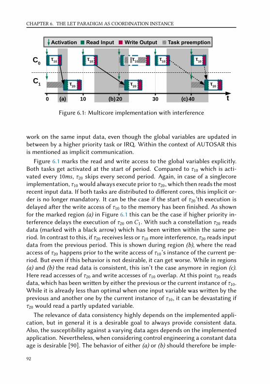
CHAPTER 6. THE LET PARADIGM AS COORDINATION INSTANCE
C0
0 10 20
C1
t
τ10
30 40
τ10
τ20
τ10
τ20
τ20
Activation Read Input Write Output Task preemption
(a) (b) (c)
τ10
τ10
Figure 6.1: Multicore implementation with interference
work on the same input data, even though the global variables are updated inbetween by a higher priority task or IRQ. Within the context of AUTOSAR thisis mentioned as implicit communication.
Figure 6.1 marks the read and write access to the global variables explicitly.Both tasks get activated at the start of period. Compared to τ10 which is acti-vated every 10ms , τ20 skips every second period. Again, in case of a singlecoreimplementation, τ10 would always execute prior to τ20, which then reads the mostrecent input data. If both tasks are distributed to dierent cores, this implicit or-der is no longer mandatory. It can be the case if the start of τ20’th execution isdelayed aer the write access of τ10 to the memory has been finished. As shownfor the marked region (a) in Figure 6.1 this can be the case if higher priority in-terference delays the execution of τ20 on C1. With such a constellation τ20 readsdata (marked with a black arrow) which has been wrien within the same pe-riod. In contrast to this, if τ20 receives less or τ10 more interference, τ20 reads inputdata from the previous period. This is shown during region (b), where the readaccess of τ20 happens prior to the write access of τ10’s instance of the current pe-riod. But even if this behavior is not desirable, it can get worse. While in regions(a) and (b) the read data is consistent, this isn’t the case anymore in region (c).Here read accesses of τ20 and write accesses of τ10 overlap. At this point τ20 readsdata, which has been wrien by either the previous or the current instance of τ10.While it is already less than optimal when one input variable was wrien by theprevious and another one by the current instance of τ10, it can be devastating ifτ20 would read a partly updated variable.
The relevance of data consistency highly depends on the implemented appli-cation, but in general it is a desirable goal to always provide consistent data.Also, the susceptibility against a varying data ages depends on the implementedapplication. Nevertheless, when considering control engineering a constant dataage is desirable [90]. The behavior of either (a) or (b) should therefore be imple-
92

6.1. THE LET PARADIGM
mented for an application, but not a mixture of both.A possible mechanism to implement the desired behavior could be based on
additional locks. This way a task starts its execution only if the logical precedingtask of the eect chain finished its execution. While such a behavior can directlybe enforced by the scheduler on a singlecore, a comparable mechanism is notfor free on a multicore. Instead, additional communication between multiplecores is needed in order to provide a flexible cross-core locking. While the codeoverhead for the additional functionality is negligible, the runtime overhead ismore important, especially as such a mechanism is either based on ineicientpolling or additional IRQs.
Within this chapter we consider a dierent lock-less method based on the socalled Logical Execution Time. The work presented in this chapter is primarilybased on the publications [27] and [25] as well as on a contribution to [35, 44]. Forthe sake of simplicity we describe the integration based on a standard task setupwithout an additional virtualization. Nevertheless, the described mechanismsshould also work for a system with multiple virtualized applications on the sameECU.
6.1 The LET Paradigm
The first reference to the LET paradigm can be found in the origins of the Giooprogramming language [61]. General idea of Gioo was to provide an abstractionlayer between control applications and the execution environment. It definestime-triggered sensor readings and task activations as well as dierent executionmodes. Access to input or output values is performed through so called driversat specified points in time.
[61] describes the design flow for a Gioo based system as follows. Firstthe control algorithm is designed according to methods already mentioned Sec-tion 2.2.1. With the use of code generation, the tested control algorithm is im-plemented in an application for later integration. Next, a hard- and sowareindependent Gioo description defines the temporal behavior of the designedapplication. This includes the specification when drivers or applications shouldbe executed. The configuration is passed to the Gioo compiler, which generatesa binary file based on the used specification. In order to execute the applicationaccording to the generated description, Gioo provides in its execution environ-ment two dierent components called E-Machine [62] and S-Machine [63]. TheE-Machine interprets the generated Gioo binary and coordinates the activationof either drivers or applications. At this point, the E-Machine is responsible forthe temporal coordination but not for the actual execution. This is done by the S-Machine which then executes drivers or applications according to the commands
93

CHAPTER 6. THE LET PARADIGM AS COORDINATION INSTANCE
from the E-Machine. In order to map this behavior to our known model, theS-Machine provides the same functionality as an OS, while the E-machine gen-erates task activations. Some more implementation details of the Gioo baseddesign flow can be found in [60].
A by-product of the development of Gioo was the LET paradigm, which ab-stracts the access to in- and output variables from the actual execution. The ideais motivated by the fact, that the behavior of an application within the real-timedomain heavily depends on the actual points in time when in- and outputs areread or wrien [74]. Therefore, the LET paradigm describes fixed points in time,when in- or outputs are read or wrien completely independent of the underlyinghard- or soware. In the context of LET, oen two other paradigms are addressedfor comparison [73]. The first one is called Zero Execution Time (ZET). The ZETparadigm assumes, that a task (or program) executes in zero time and thereforewithout any delay between read, execution and write. This model seems to benot realistic at first glance, as a task always needs some time for execution. Onthe other hand, this model corresponds exactly to the behavior of simulationsoware like MATLAB/Simulink which we described in Section 2.2.1.
The second paradigm is called Bounded Execution Time (BET) and describesthe well-known behavior as covered by classic real-time analysis. A task mightneed some time aer activation to produce a result, but this time is upper boundedto a certain value. This is exactly the behavior described by Section 3.2. Convert-ing the BET to our used system model results in the WCRT. This means, thatan upper bound for write accesses at the end of a task exists, but early write ac-cesses based on lower interference than the worst case would not be enforced.The example from Figure 6.1 already showed that such a behavior might causeproblems.
As already mentioned the LET paradigm defines explicit points in time forread and write access. It is a mixture of both, ZET and BET. The LET appliesfixed points in time for read and write, while allowing an BET behavior for theremaining part of the application. An example for LET is shown in Figure 6.2with a task τ . The upper half of the Figure 6.2 shows the LET abstraction which
τ
t
LET
WRLET Abstraction
Scheduled Task
BET
Figure 6.2: Logical execution time of τ
94
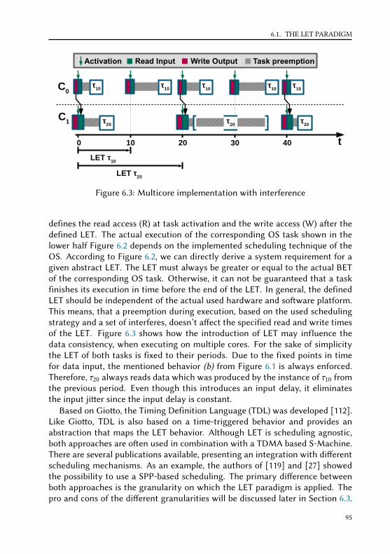
6.1. THE LET PARADIGM
C0
0 10 20
C1
t
τ10
30 40
τ20
Activation Read Input Write Output Task preemption
τ10
τ10
τ10
τ10
τ20
τ20
LET τ10
LET τ20
Figure 6.3: Multicore implementation with interference
defines the read access (R) at task activation and the write access (W) aer thedefined LET. The actual execution of the corresponding OS task shown in thelower half Figure 6.2 depends on the implemented scheduling technique of theOS. According to Figure 6.2, we can directly derive a system requirement for agiven abstract LET. The LET must always be greater or equal to the actual BETof the corresponding OS task. Otherwise, it can not be guaranteed that a taskfinishes its execution in time before the end of the LET. In general, the definedLET should be independent of the actual used hardware and soware platform.This means, that a preemption during execution, based on the used schedulingstrategy and a set of interferes, doesn’t aect the specified read and write timesof the LET. Figure 6.3 shows how the introduction of LET may influence thedata consistency, when executing on multiple cores. For the sake of simplicitythe LET of both tasks is fixed to their periods. Due to the fixed points in timefor data input, the mentioned behavior (b) from Figure 6.1 is always enforced.Therefore, τ20 always reads data which was produced by the instance of τ10 fromthe previous period. Even though this introduces an input delay, it eliminatesthe input jier since the input delay is constant.
Based on Gioo, the Timing Definition Language (TDL) was developed [112].Like Gioo, TDL is also based on a time-triggered behavior and provides anabstraction that maps the LET behavior. Although LET is scheduling agnostic,both approaches are oen used in combination with a TDMA based S-Machine.There are several publications available, presenting an integration with dierentscheduling mechanisms. As an example, the authors of [119] and [27] showedthe possibility to use a SPP-based scheduling. The primary dierence betweenboth approaches is the granularity on which the LET paradigm is applied. Thepro and cons of the dierent granularities will be discussed later in Section 6.3.
95

CHAPTER 6. THE LET PARADIGM AS COORDINATION INSTANCE
In contrast to the previous integration, the authors in [46] showed, that also EDFscheduling can be applied in the S-Machine. As we consider primarily the au-tomotive domain, an EDF-based scheduling is less relevant than SPP, which isthe desired scheduling strategy in OSEK and AUTOSAR OS. In general, it is de-sirable not to change the current SPP as this would entail major changes in thedesign process. However, this approach does only allow communication at taskboundaries, which leads to long response times on eect chains across severalcores. Even in case of a parallel execution this may lead to long end-to-end la-tencies as shown in [18]. The authors of [48] proposed to keep that schedule andchange the role of the LET requirements. Instead of using the WCRT as lowerbound for the LET, they change the worst case model of to a typical worst casemodel allowing shorter LET at the cost of a formally bounded number of LET (i.e.deadline) misses. [119] also justifies this for control loop properties.
Recent work considering LET in the automotive domain primarily target theanalysis of eect chains. Primary driver for this idea is the fact that LET re-moves the input jier and improves the predicabilty. The industrial motivatedWATERS challenge in 2017 [54] compared dierent eect chain analysis meth-ods for dierent communication types, including a LET-based shared memorycommunication. The dierent contributions [52, 83, 32, 34] showed analyticalapproaches, for end-to-end timing delays. Some workshop contributions havelater been expanded to full conference publications [82, 31]. In general a goodoverview of currently existing analysis methods is given in [22].
6.2 Lock-less Zero-Time Communication
While the theoretical benefits of LET has been widely discussed, the actual im-plementation and integration into an existing automotive OS has been largely ig-nored so far. Only a few publications [98, 31, 46] consider actual implementationaspects. Crucial is the implementation of the timed communication at the LETboundaries, which should be performed in zero-time according to the LET para-digm. While providing a robust theoretical framework with atomic data trans-fers, implementing a zero-time communication is not straight forward. First ofall, an execution time equal zero is simply not possible for a data copy operationon a processor. A copy operation always takes some time, even if it is performedvia a dedicated DMA controller. Second, the execution for dierent payload sizestimes for read/write accesses vary. As read/write accesses should be executed ona privileged level to ensure data consistency, the entire system is preempted forsuch accesses. This means, that long execution times for large data chunks to becommunicated would represent a not negligible overhead.
In order to provide a zero-time communication, this section describes a simple
96

6.2. LOCK-LESS ZERO-TIME COMMUNICATION
mechanism with limited overhead. General idea is to use a double buering forvariables with cross core dependencies. This is based on the fact, that in the au-tomotive domain a classic publisher subscriber paradigm with global variables isused for ECU internal communication, as already mentioned in Section 2.2.1. Avariable is therefore only wrien/updated by one task (publisher), while it mightbe read by several other tasks (subscribers). The basic functionality of the pro-posed mechanism operates in the following manner. For each cross core de-pendent variable a double buer with twice the memory of the correspondingvariable exists. One half of this double buer is used for read (subscriber) andthe other half for write (publisher) accesses. Publisher and subscriber access thedouble buer through distinct pointer for write and read access. At the end ofeach publisher’s LET read and write pointer then get swapped. The previouswrite buer is now used as read buer and vice versa.
An example for this mechanism with one publisher and two subscribers isgiven in Figure 6.4. R and W are the pointers used for read and write access.We use a C-style syntax with an * to indicate the actual access to the memoryreferenced by the corresponding pointer. Therefore, both rows for R* and *Win Figure 6.4 show the actual content of the referenced memory, which changesover time due to write accesses or pointer swaps. In contrast to the behavior de-fined by the LET paradigm, the actual memory accesses performed by the tasksare still performed bounded to the actual execution of the task. Due dierentinterference, the memory access is not fixed to certain moment in time. Never-theless, because of the double buering, including pointer indirection and swap,it occurs to all subscribers as if the publisher acts according to the LET paradigm.The memory access can therefore be performed in the same context of the corre-sponding task and does not need to be treated separately. In order to achieve thiseect, the mechanism needs to enforce early write and delayed read accesses.
The enforcement of an early write behavior is shown in Figure 6.4. The pub-lisher τ0 is executed on C0, the two subscribers τ1 and τ2 on C1 and C2. For thesake of simplicity we omit the read accesses during τ0 and write accesses duringτ1/τ2, as those are not relevant for the shown example. The publishing task τ0starts execution and finishes with a write access. From t0 . . . t1 τ0 writes c tothe buer through the dereferenced write pointer *W. As the LET of τ0 has notyet been finished, the published variable must not be visible to other subscrib-ing tasks. Next, τ1 starts execution and accesses the referenced address from theread pointer *R at t2 and reads b from the read buer. Although new data hasalready been wrien at t1 it is not visible for a subscriber until t3, which is com-pliant to LET paradigm. At t3 read and write pointer get swapped and thereforethe read pointer now references the data buer that contains c. If subscriber τ2now accesses the read buer at t4 it reads the new data c which was wrien att1 and published at t3. The other buer, holding data b, is now referenced by the
97

CHAPTER 6. THE LET PARADIGM AS COORDINATION INSTANCE
c ba d
cb
C0
t
C2
C1
τ0 c
τ1b
τ2c
*R
*W
t0 t1 t2 t3 t4
τ0 d
t5 t6
LET Boundaries
Task preemption
Read via *R
Write via *W
Figure 6.4: Zero-Time Communication early write enforcement
write pointer and gets therefore overwrien at the next write access of τ0 from t5. . . t6. Like in Figure 6.4, the tasks might also get preempted in Figure 6.2. As longas they are able to finish their execution, including the needed time for read andwrite accesses, everything is fine. The zero-time communication implementationwith a double buering is therefore entirely scheduling agnostic, as required bythe LET paradigm.
The first implementation of this mechanism mentioned in [27] only enforcedan early write behavior, which can be suicient for certain system configura-tions. This means, the system does not care when the actual data is wrien by apublisher, as the zero-time communication is performed with the pointer swap.Nevertheless, this simple measure is not suicient if LETs of dierent tasks over-lap. According to the definition of the LET paradigm, the read access is performeddirectly on task activation. We already mentioned for the previous example inFigure 6.4 that also the read access is performed in the task’s context. Due tointerference from other tasks or additional IRQ handling, this read access mightnot be performed directly at task activation, While this isn’t a problem in theexample from Figure 6.4, this changes if the actual task execution is delayed be-yond the LET boundary of the publishing task. Figure 6.5 shows an example forthis behavior.
Again the example in Figure 6.5 uses a publishing task (τ0) on C0 and twosubscriber on C1 (τ1) and C2 (τ2). At t0 τ0 finishes its execution and changes the
98

6.2. LOCK-LESS ZERO-TIME COMMUNICATION
b dca
cb
C0
t
C2
C1
τ0 c
τ1b
τ2c
*R
*W
t0 t1 t2 t3 t4
τ0 d
LET Boundaries
Task preemption
Read via *R
Write via *W
Figure 6.5: Zero-Time Communication delayed read enforcement
data referenced by *W to c. The LET of both subscribing tasks τ1 and τ2 startat t1. Both tasks are initially delayed. τ1 performs therefore a read access at t2and reads b, which is the correct data value according to the LET paradigm. Att3 the LET of τ0 ends and the previously wrien data is published. When τ2 nowaccesses the read buer at t4 it reads the value c published at t3. This is wrongaccording to the LET paradigm, as the LET of τ2 has started while the read buercontained b. In order to fix this, it is suicient to create a read pointer backupat the start of the corresponding LET (e.g. at t1). This way τ2 would access thecorrect buer at t3. In a system where the publishers period is way shorter thanthe period of a subscriber, also a simple double buer is not suicient. Due tothe publishers short period, previously wrien data would simply be overwrientoo soon.
Figure 6.6 shows how the previously described behavior can be enforced witha simple ring-buer implementation storing more than two version of a variableat a time. Let us assume, that τ1 and τ2 read data, wrien by τ0 and the ring-buer rb is able to store four entries. τ1 is activated with an oset relative τ0, butthe period (and in this example also the LET) of both is still the same. As a result,τ1 reads each value, wrien by τ0 in the previous period. In contrast to this τ2 hasa three times longer period than τ0. Therefore, during the LET of τ2, τ0 producesthree new output values which need to be stored at dierent locations in order topreserve the desired delayed read behavior. In Figure 6.6, the LET of τ2 starts at t1.
99

CHAPTER 6. THE LET PARADIGM AS COORDINATION INSTANCE
b
τ1
aa
C0
t
C2
C1
τ0 b
τ1a
τ2b
rb[0]
t0 t1 t2 t3
τ0 c
LET Boundaries
Task preemption
Current R
Current W
τ0 d τ
0 e
τ1b τ
1c τ1d
rb[1]
rb[2]
rb[3]
y
b
cc
z d
R‘ = R &rb[0] R‘ = R &rb[1] R‘ = R &rb[2] R‘ = R &rb[3]
R‘ = R &rb[1]
W = &rb[1] W = &rb[2] W = &rb[3] W = &rb[0]
x b
e
d
c
Read via *R‘
Write via *W
Figure 6.6: Zero-Time Communication based on ring buer
The relevant input value from τ0 was therefore produced between t0 and t1. In ourexample τ0 writes b to the ring-buer entry rb[1], which becomes visible to τ2 att1. At t1 the LET of τ2 begins and an internal copy (R’) of the current read pointer(R) is generated. Within the shown example the execution of τ2 is delayed dueto high priority interference on C2. Due to the local read pointer copy (R’) andthe multiple entries in the ring-buer, τ2 still reads the correct value (b) when itstarts execution. Even though τ0 had already produced new output data at t2 andt3, the desired delayed read behavior according to the LET paradigm is ensuredthis way.
While enforcing a delayed read behavior is comparatively simple, it is heavilyapplication dependent if this is even necessary. For some applications in controlengineering it would be preferable to always take the most recent value as inputdata. Otherwise, a phase shi might be introduced, leading to possible instabil-ity of the controlled system [90]. Therefore, although the LET paradigm dictatesimplicitly when data shall be read, it should be optional for an application if a de-layed read behavior is enforced or not. Multiple LETs can also be aligned in way,such that an explicit delayed read enforcement mechanism is not needed. Againthis is heavily application dependent. Therefore, the user has the opportunity todecide if an enforcement is used or not in the later explained implementation.
100

6.3. LET IN AUTOMOTIVE SOFTWARE
6.3 LET in Automotive Soware
The LET paradigm has already been considered by several automotive OEMsand soware suppliers [44] to be a useful coordination instance. Nevertheless,there are dierent views on how LET can be applied to existing soware. In thiscontext there are two primary points of contention. First the soware granularityon which LET should be applied and second the temporal dimensioning of LETsizes. Resulting of both are two major interpretations of LETs applicability toautomotive domain.
The first interpretation directly applies LET to existing soware with the aimof achieving maximal flexibility. As a result, the LET paradigm is directly ap-plied on existing tasks without further optimization regarding osets or paral-lelizability. With an LET equal to the tasks period the system setup does notchange from an OS perspective which is explained in this section. This interpre-tation is primarily driven by the authors of [119] and will be referred as macro-LET in the remainder of this document. The majority of the related work from[52, 83, 32, 34, 82, 31, 22] is based on this LET interpretation. The second interpre-tation applies LET on a smaller granularity to an optimized schedule. Result is ause-case optimized schedule, with much smaller LETs. This second interpretationis proposed primarily by the authors of [59] and will be referred as micro-LET inthe remainder of this document. Even though, both interpretations are based onthe same LET paradigm, major dierences, especially regarding the implemen-tation, exist.
One major dierence between macro and micro LET, is the way how existingapplication tasks are mapped to LET tasks and dierent cores. At this point it isimportant to point out that we distinguish between actual application tasks τischeduled by an OS and LET tasks λi . In our context a LET task is only a temporalframe that implicitly defines the communication (read input, write output). Anapplication task is, as already mentioned in Section 2.2.1, implemented as a setof runnables executed in a static order. Oen, the runnables can be grouped intobasic blocks, which only share intermediate data dependencies.
Considering the mapping between application and LET tasks, it is straight for-ward in case of macro-LET. For each application task only one LET task is used.According to [119] an already existing application task from a singlecore imple-mentation should not be executed in parallel on dierent cores. Instead, entireapplication tasks might be placed on dierent cores. In some cases it might makesense to spilt an existing application task to multiple cores, but this is usually tobe avoided due to unknown dependencies in existing legacy soware. Both, map-ping to LET tasks and multicore distribution is therefore preferably performed ona task granularity. In contrast to this the micro-LET approach proposes a par-allel execution of independent basic blocks. Therefore, LET tasks are mapped to
101

CHAPTER 6. THE LET PARADIGM AS COORDINATION INSTANCE
τ10
τ20
f3 f4 f5 f7 f8f1 f2 f6
(a) Singlecore mapping
C0
0 10 20
C1
t30
Activation Read Input Write Output Task preemption
λ10
λ20
f3 f4 f5f1 f2
f7 f8f6 f7 f8f6
f3 f4 f5f1 f2 f3 f4 f5f1 f2
(b) Multicore implementation macro-LET
C0
0 10 20
C1
t30
λ10,0
f3 f4
f5
f1 f2 f7
f8f6
f3 f4
f5
f1 f2 f3 f4
f5
f1 f2 f7
f8f6
λ10,1
λ20,0
λ20,1
λ10,2
λ20,2λ
10,0
λ20,0
(c) Multicore implementation micro-LET
Figure 6.7: Comparison of LET task mapping for macro- and micro-LET
smaller basic blocks instead of entire tasks. This implicates that one applicationtask might be mapped to multiple LET tasks. [59] describes how such a mappingbased on a singlecore implementation can be performed.
In order to explain the dierences even further Figure 6.7 provides a simpleexample. First, Figure 6.7a shows the original tasks used for the singlecore im-plementation, with two dierent eect chains. The first chain is f1 → f2 →f3 → f4 → f6 → f7 (blue) and the second one is f1 → f2 → f5 → f6 → f8(red). Therefore, both chains share the runnables f1, f2 and f6. Figure 6.7b showshow this example could be mapped under the consideration of macro-LET. Thepreviously used tasks are distributed to dierent cores and the LET of each taskis set equal to its period. In contrast to this Figure 6.7c shows the mapping underthe consideration of micro-LET. Instead of one big LET task, both application
102
6.3. LET IN AUTOMOTIVE SOFTWARE
tasks have been divided into three smaller basic blocks according to the desireddataflow based on the eect chains, with a distinct LET task per basic block. As aresult, independent basic blocks like (f3, f4) and f5 can be executed in parallel ondierent cores. Due to the smaller distribution granularity based on the acquiredbasic blocks, the corresponding LETs are also shorter.
When designing LET based systems, the end of a task’s LET is conterminousto a task deadline. In order to check the correctness of a designed system itmust be ensured, that each task is able to finish execution during its LET. In caseof macro-LET nothing changes compared to the previous system setup, as thedefined LETs are equal to the task’s periods. Since the previous system setupwas RMS based, nothing changed with respect to task deadlines. Therefore, thesystem can simply be analyzed with the existing RTA methods. Only the task setson distinct cores dier from the previous setup due to the multicore execution.
In case of micro-LET this is a dierent, as basic blocks and the correspond-ing LETs are much shorter now. An additional requirement for the micro-LETapproach according to [59] is, that the execution of all LET managed applica-tion tasks must fit into the smallest period. For the example in Figure 6.7 thismeans, that the execution of τ10 and τ20 must be finished within the period ofτ10. Otherwise, the assignment of the shown micro-LET slots would not be pos-sible. Since all LET-based tasks (e.g τ10 & τ20) are now synchronized, they don’tinterfere anymore on the same resource. Even though the micro-LET slots mightlook like a TDMA based system, it isn’t the case. The micro-LET slots do only de-fine a temporal region for execution without any impact on the actual schedulingpolicy.
We already mentioned that a task’s WCRT denotes a lower bound for a pos-sible LET. The only dierence in case of micro-LETs is that the WCRT is calcu-lated for a smaller execution time with a reduced set of interferes. Analyzing amicro-LET based system is then straight forward. Regarding the example fromFigure 6.7c, this leads to
Cτ10,0 = Cf1 +C f2 → Rτ10,0 ≤ λ10,0
Cτ10,1 = Cf3 +C f4 → Rτ10,1 ≤ λ10,1
Cτ20,1 = Cf7 → Rτ20,1 ≤ λ20,1
for C0 and to
Cτ10,2 = C f5 → Rτ10,2 ≤ λ10,2
Cτ20,0 = C f6 → Rτ20,0 ≤ λ20,0
Cτ20,2 = C f8 → Rτ20,2 ≤ λ20,2
forC1. We define for each coreCi two sets of LET tasks. The first setΛi ,ϵ includes
103

CHAPTER 6. THE LET PARADIGM AS COORDINATION INSTANCE
λi
τi
Ri S
i
BACT
BHP,i
Figure 6.8: Interference during execution inside LET boundaries
all LET tasks used for the execution of basic blocks on core Ci . The second setΛi ,δ includes all LET tasks used to oset basic blocks for synchronous executionon dierent cores. For the example from Figure 6.7c this results in:
Λ0,ϵ = λ10,0, λ10,1, λ20,1 Λ0,δ = λ20,0
Λ1,ϵ = λ10,2, λ20,0, λ20,2 Λ1,δ = λ10,0
In order to check schedulability for the constructed schedule the sum over Λi ,ϵand Λi ,δ must be smaller or equal than the used minimum period on each core∑
λ∈Λi ,ϵ
λ +∑
λ∈Λi ,δ
λ ≤ minτj ∈Γi ,LET
Pj (6.1)
where Γi ,LET contains all application tasks, executed and decoupled within LETboundaries.
Even though there are obvious dierences between macro- and micro-LET, theRTA is still the same. Both approaches can be analyzed with the busy-windowfrom Section 3.2. The only dierences are as mentioned above the mapping gran-ularity and the interfering task-set. In general, the execution of a task or basicblock follows the example from Figure 6.8. Aer activation, the execution of atask initially delayed, based on the LET implementation. This activation delay ismarked as BACT in Figure 6.8. Additionally, also blocking based on higher prior-ity interference (BHP ,i ) needs to be accounted. At this point BHP ,i can be basedon higher priority task or additional IRQs for peripheral hardware. The genericblocking Bi (∆t) from Definition 3.15 can then be replaced with:
Bi (∆t) = BACT + BHP ,i (∆t)
While BHP ,i depends on the actual task-set, BACT highly depends on the imple-mentation framework. Therefore, the evaluation in Section 8.2.1 shows how anaccurate value can be determined for the proposed implementation frameworkfrom Section 7.2.
104

6.3. LET IN AUTOMOTIVE SOFTWARE
Macro-LET Micro-LETLET task mapping 1xτ → 1xλ 1xτ → nxλ
LET sizes λ = P λ ≤ P
Input jier 0 0
End-to-end latencies . . . ≥ Singelcore ≤ SingelcoreScheduling slack Usually large Usually smallSusceptibility underincreased load Potentially low Potentially increased
Flexibility Flexible Static (use-case optimized)
Table 6.1: Comparison table of macro- and micro-LET
Table 6.1 shows a comparison of macro- and micro-LET. First of all, the pri-mary dierences between both approaches are the task mapping and the LETsizes. While macro-LET proposes a direct mapping between application and LETtasks with LET sizes equal to the task periods, micro-LET proposes a much finergranularity with much shorter LET sizes. As a result of this dierent LET sizes,such systems behave dierent in many ways. First, the end-to-end latencies ofeect chains. The example from Figure 6.7 shows directly the dierence betweenboth regarding end-to-end latencies. In Figure 6.7b τ10 and τ20 get activated att = 0. Even though τ20 on C1 starts executing aer the LET of first the instanceof τ10 onC0 finishes at t = 10, the freshly created output value will be discarded.Instead, an older value from t = 0 is used during the execution of τ20. Comparedto a singlecore execution where τ20 would start execution right aer τ10 has fin-ished (due to RMS based scheduling), the end-to-end latencies with macro-LETmay increase. This has already been observed in [52]. In contrast to this, themicro-LET approach allows an optimized basic block placement with dierentoset. This way, the same end-to-end latency compared to a singlecore imple-mentation can be achieved. Additionally, if possible the parallel execution ofindependent blocks allows to shorten the end-to-end latency even more.
Second and third, the available scheduling slack and resulting from this thesusceptibility under increased load. In case of macro-LET this is straight forward,as nothing really changed compared to the singlecore implementation exceptthat less interfering tasks may share the same core. As defined in Definition 3.17the slack is given as dierence between deadline and response time. Since dead-line, period and LET are equal in case of macro-LET, the slack stays more or lessthe same compared to a singlecore implementation. It’s even more likely thatthe amount of slack grows, since interference from higher priority tasks mightbe removed due to execution on a dierent core. Resulting from the potentiallyincreased slack, a macro-LET based system is more robust and tolerates more ad-ditional load from unpredictable sources (like peripheral IRQs). The maximum
105

CHAPTER 6. THE LET PARADIGM AS COORDINATION INSTANCE
amount of additional allowed load/interference can be calculated on the nor-malized slack during execution within LET boundaries. The minimum availablenormalized slack Smin over all available LET tasks defines the maximum allowedinterference.
Smin = mini ∈Γ
Riλi
(6.2)
Without any information about the additional interference (e.g. if it is alignedwith the scheduling) this must apply to any time window of size ∆t = λi . Thislimitation for additional load is also valid in case of micro-LET. Due to the shorterbasic blocks and LET sizes the absolute amount of slack decreases. Even normal-ized to the LET sizes, this amount of slack in a micro-LET based system is usuallysmaller compared to macro-LET. Primary reason for this is the LET task mappingwhich optimizes the end-to-end latencies. As already mentioned, this implicatesthat all LET tasks must be able to finish within the smallest period of the appli-cation tasks. In general this leads to a smaller normalized slack and therefore toa system which is much more prone to deadline (or LET) misses when dealingwith additional loads from unpredictable sources. From the available slack andthe susceptibility under increased load directly the system flexibility can be de-rived. One of the primary constraints during the design of the original LET para-digm [74] was to create hardware and OS agnostic application soware whicheasily can be migrated to a completely dierent execution platform. Therefore,in the original LET proposal changing the execution environment must have noeect on the actual LET sizes. While the integration of LET in the automotive do-main does not directly aim for maximal independence between application so-ware and execution platform, it makes sense to be aware about the limitationsof macro- or micro-LET regarding the system flexibility. Based on the previousobservations, macro-LET usually provides a much more flexible system due toadditional slack. Therefore, it is more likely that in case of a macro-LET basedsystem it is much more straight forward to change/add soware parts or mod-ify/change the execution environment, without any modifications on the LETsizes. In contrast to this, a micro-LET based system is much more static due tothe optimized schedule resulting in less slack and flexibility.
Even though, macro- and micro-LET show larger dierences, both approachescan be realized with the proposed zero-time communication with either double orring buering. Important is in both cases that the implementation provides a lowand constant runtime overhead. The memory architecture of the used µC/SoCgets also important, when considering the placement of double or ring buers.Those aspects depend highly on the actual implementation and will therefore befaced in the following chapter.
106

CHAPTER7
Implementation Challenges
“So, no more running. I aim to misbehave.”
- Malcom Reynolds
Implementation challenges of mechanisms like the proposed SPS based budgetscheduling or the LET synchronization are oen neglected in the academic world.Reason for this is the very time-consuming implementation based on complexhardware and comprehensive soware frameworks. Since implementation heavypapers are usually hard to publish, the additional eort of a “real-world” imple-mentation is oen avoided. While this is absolutely understandable for a PhDstudent with limited time, it still leads to a gap between academic research andactual problems in the industry.
When designing schedulers or other OS mechanisms, there are several limitedresources on embedded systems which need to be considered. As an example, thediscussed mechanisms from the previous chapters need both an accurate timebase. An operating system itself usually provides a periodic system tick. Thegranularity of this system tick is oen in the range of 1ms . Since the systemtick is based on a dedicated hardware timer, an IRQ is generated for each tick.Therefore, much smaller granularities than 1ms are oen avoided due to highIRQ loads. For the discussed mechanisms from previous chapters, a granularityof 1ms might not be suicient. As a result, additional timer hardware is needed.
We already mentioned in Section 2.1 that PWM is widely used in embeddedsystems for dierent purposes. As result, the generation of such signals is done
107

CHAPTER 7. IMPLEMENTATION CHALLENGES
CV
PWM Period Counter
t
Top
1IO
0t
Duty Cycle
Figure 7.1: Generation of a PWM signal
by distinct peripheral in nearly every modern µC/SoC. The way how the signalgeneration is achieved is more or less identical in all cases and is shown in Fig-ure 7.1. A free running timer (oen also mentioned as counter) counts upwardsto a certain Top value, wraps around to zero and continues operation. In somecases the top value can be specified by an additional register, but oen the topvalue is given by the maximum bit size of the timer’s hardware implementation.The time it takes to count from zero to the top value is mentioned as PWM Periodwhich can be varied by the timers frequency and/or the top value itself. In orderto generate a PWM signal an additional register is used which contains a com-pare variable CV. The actual state of the output IO is then coupled to a compareoperation, e.g. as long as the current timer value is smaller than CV the outputis set to 1, otherwise it is set 0. Changing CV does than directly influence thePWM Duty Cycle.
Beside the PWM generation, such timers are usually multi functional. Theoutput signal generation can be usually disabled and the timer can be config-ured to generate an IRQ when the timer value is equal to CV. This way a freerunning timer can be used to generate highly accurate timed IRQs. Additionally,they can be used for fine granular time measurement. The maximum time thatcan lay between two consecutive generated IRQs or can be measured betweentwo events, is in both cases limited to the timers period (PWM Period). ModernµCs/SoCs like the AURIX or R-Car H3 provide multiple timers with such a func-tionality, oen with more than one compare register. Nevertheless, it is desirableto use such hardware timers as eiciently as possible in order to still provide fur-ther timer modules to the application.
108

Listing 7.1: Task state check with if
1 int check_taskstate(TCB_T *pTcb)2 3 if(pTcb ->State == READY)4 return 0;5 if(pTcb ->State == RUNNING)6 return 1;7 if(pTcb ->State == SUSPENDED)8 return 2;9 if(pTcb ->State == WAITING)
10 return 3;1112 return -1;13
Listing 7.2: Task state check with switch
1 int check_taskstate(TCB_T *pTcb)2 3 int ret=0;4 switch(pTcb ->State)5 6 case READY: ret = 0; break;7 case RUNNING: ret = 1; break;8 case SUSPENDED: ret = 2; break;9 case WAITING: ret = 3; break;
10 default: ret = -1; break;11 12 return ret;13
Beside the limited peripheral resources, also some basic rules should be con-sidered when developing mechanisms targeted for the implementation in smallRTOSs. In general a small overhead regarding code size, data and runtime over-head is desirable. While a small runtime overhead for an OS is advantageous, aconstant runtime overhead is much oen more important. A constant runtimeoverhead is easier to integrate in a RTA and leads overall to a much more pre-dictable system behavior. In case of OSs, task state dependent decision taking is amajor functionality. A simple example for such a decision is shown in Listing 7.1.With several if -statements the state of a task is checked based on its TCB andthe function returns with a corresponding value. If the task is in an invalid state,an error (−1) is returned. The functionality of such a function is straight forwardand the code is easy to understand. Nevertheless, in case of a RTOS an imple-mentation like in Listing 7.1 should be avoided since the runtime depends onthe task state. Instead of an implementation based on multiple if -statements, aswitch based solution like in Listing 7.2 is desirable. A switch-statement is usuallycompiled to a lookup based jump table, which results in a constant runtime foreach state decision. Even though the simplicity of the used example, such statebased decisions are widely used, also in case of entire state machines. Aware-ness of the discussed runtime variation between both implementation methodsis therefore a key feature when implementing such RTOS mechanisms.
In some cases a constant runtime overhead in an RTOS mechanisms is hardto achieve. This may be based on the mechanisms itself, but oen a constantruntime overhead is exchanged against flexibility. As an example, during theevaluation we will use two dierent RTOSs with SPP based scheduling calledµC/OS-II [68] and ERIKA OS [51]. While the entire design of µC/OS-II is opti-mized for this kind of scheduling, ERIKA OS can be configured for several otherscheduling strategies (e.g. EDF). This dierence directly influences the way howthe SPP scheduling is implemented in both RTOSs. In case of µC/OS-II a highlyoptimized mechanism is used, which implements the SPP scheduling with a con-stant runtime overhead. In contrast to this ERIKA OS uses a flexible systembased on ready queues. A ready queue contains all tasks which are ready forexecution and the dispatcher simply reads and executes the task referenced by
109

CHAPTER 7. IMPLEMENTATION CHALLENGES
the first queue entry. The only thing, which diers between several schedulingstrategies is the function which inserts new tasks to the queue. In case of a prior-ity based scheduling the first entry of this queue always contains the task withthe highest priority. While the overhead when reading a task from the queue isconstant, adding a new task to the queue produces a variable overhead due tosorting inside the queue.
Therefore, ERIKA OS exchanges predictability against flexibility, when com-paring it against µC/OS-II. The argumentation how this can be tolerated in aRTOS is, that the maximum runtime overhead has an upper bound. This is thecase for the described ready queues from ERIKA OS since the number of tasks in-side the system does not change over runtime (and is limited by the OSEK and/orAUTOSAR OS definition). Regarding the constant runtime overhead this means,if a constant runtime overhead can not be ensured during runtime by implemen-tation, it should be upper bounded during compiletime through a parameter.With this general ideas in mind, we will now discuss the implementation of thepreviously described scheduling mechanismsm from Chapter 4, Chapter 5 andChapter 6. The work presented in this chapter is therefore based on [26, 24] and[27, 25, 7].
7.1 SPS based Budget Scheduling
Figure 7.2 shows the proposed SPS based architecture, which was already men-tioned in Section 5.1.1. It consists of two major parts, first the SPS for interfer-ence enforcement and second the scheduler for service provisioning. The inter-action between both is realized with a CB API, which is explained further in Sec-tion 7.1.2. The SPS has four incoming signals, which primary define the runtimebehavior. Those signals are, as already discussed in Section 5.1.1, Empty, Refill,Idle and Resume. Empty and Refill are IRQs based on a timer module, which isunder the control of the SPS. The interrupts indicate either an empty budget ora budget replenishment/refill. Therefore, the proper configuration of the timermodule is the main component to enforce interference. Due to the importanceof the timer module, we explain this component further more in Section 7.1.1.
When a partition served all its outstanding activations, an Idle signal can besent to the SPS. The way how we realized this signal is based on an additionalsystem call. This system call is issued by a partition when it enters its idle loopor idle task. Depending on the actual hardware, system calls may be executeddierently. Nevertheless, a system call is always handled within a specific con-text of the CPU. If this is realized with a distinct context only for system calls orwithin a shared context (e.g. shared with hardware IRQs) depends on the actualused CPU architecture. For the sake of security it is important that the system
110

7.1. SPS BASED BUDGET SCHEDULING
Provide Service
Enforce Interference
SPS
Timer
ActivateTask
Em
pt y
Refill
SchedulerC
B A
PI
Parti tio
n
Resume
Co
ntro
l PartitionsP2
Prio
t
P1Prio
t
P0Prio
t
Dispatch
Idle
Figure 7.2: Overall architecture for SPS based scheduling
call is always handled in a dierent context than the actual execution of the par-tition. This is also the case for the Resume signal, which can be issued from anIRQ (e.g. time tick) or a system call (e.g. inter-partition communication).
When handling each of this four signals, the SPS forwards the signal to thescheduler. The decision which partition should be dispatched next, is thereforeup to the scheduler. Beside the CB API, Section 7.1.2 will also show how a simpleTDMA scheduling can be realized with the proposed architecture from Figure 7.2.Based on this simple example, Section 7.1.3 then explains the actual budget basedscheduling.
7.1.1 Timer usage
We already explained how a common PWM timer can be used for a flexible andaccurate IRQ generation. Each time the timer reaches the compare value, storedin the dedicated register, an IRQ is generated. Figure 7.2 already showed, thatthe generation of the budget Empty and Refill signals is based on a timer module.
The generation of the budget empty signal is quite obvious. Each time a parti-tion is picked for execution, an irq must be generated when the budget depletes.Since we use a free running timer (32-bit), which overflows to zero at its definedboundary the compare value for the register can be calculated as:
111

CHAPTER 7. IMPLEMENTATION CHALLENGES
DIFF
Empty Budget
Current Time
DIFF
Refill Budget
LEQ
Compare Register
Timer State
Figure 7.3: Timer compare register configuration
CompareReдister = CurrentTime + BudдetLe f t
Since all values are treated as 32-bit unsigned integers, an overflow is handledautomatically. The generation of the budget refill signal is also simple. Each timea partition stops execution, the used budget is prepared for replenishment. Asan example, when a partition executes from t0 . . . t1, the compare register is setto
CompareReдister = t0 +TR
in order to generate an IRQ at the correct point in time.A straight forward way to generate both signals would be to use two timers
with two compare registers. Since the synchronization of two timers is some-times challenging, a solution with one single timebase is oen preferable. Fig-ure 7.3 shows how both signals can be generated with only one timer and a singlecompare register. As inputs the absolute time of the current budget empty eventand the head of a budget refill queue are taken. While the absolute time of thenext budget empty event depends on the currently executed partition, the queueholds all times for future budget refill signals from partitions which have beenexecuted in the past. The queue is therefore ordered according to the absolutetimes, with the closest refill event at the head and the latest event at the tail.Each time a timer IRQ is issued or the partition context is switched, the fol-lowing lookup is performed. First, the dierence between the current time and
112

7.1. SPS BASED BUDGET SCHEDULING
both, next budget empty and next budget refill event, is calculated. Second, thesmaller value is loaded to the compare register and an internal timer state is set.The timer state indicates, if the occurred IRQ should send an Empty signal, Refillsignal or both to the SPS core module. Dependent on the sent signal the corre-sponding signal is then handled by the SPS, which is explained in more detaillater in Section 7.1.2.
We mentioned before, that the refill queue holds all times for future budgetreplenishments and is sorted accordingly. From the idea, this is comparable withthe previously discussed ready-queue and an EDF based scheduling. Reading anentry from the queue is therefore performed with a constant overhead, but theinsertion into the queue might be challenging. For our system this is not thecase as a new entry can always be appended at the end of the queue withoutviolating the chronological sorting. In order to explain this, let us assume thefollowing example with three partitions. The first partition executes from t0 . . . t1,the second from t1 . . . t2 and the third from t2 . . . t3 with t0 > t1 > t2 > t3.According to the SPS the used budgets are replenished at:
t0 +TR : t1 − t0 time units for the first partition
t1 +TR : t2 − t1 time units for the second partition
t2 +TR : t3 − t2 time units for the third partition
Because of the same replenishment period TR for all partitions in the system,the order of replenishments is always identical to the previously seen executionorder. This makes our approach much easier to implement compared to the stan-dard SPS based scheduling, where multiple replenishment periods are possible.Reason for this is, that in case of dierent replenishment periods it is not validanymore to always append entries to the end of the refill queue. Instead, theentire queue might be processed in order to find the corresponding place for thene entry. Alternatively, a distinct timer for each replenishment period could beused to overcome this issue. In reality this implementation based limitation ofthe original SPS was one reason, why the SPS has seen so lile aention in thepast. For our proposed system with only one replenishment period, the imple-mentation isn’t a problem anymore.
7.1.2 SPS CBAPI
The CB API is the connection between scheduler and SPS. It consists out of aset of primary and secondary callback functions. Each callback function returnsa partition which should be scheduled next (except the CB_Init() callback). Theprimary callbacks are directly coupled to the ingoing signals Refill, Empty, Re-sume and Idle as already shown in Figure 7.2.
113

CHAPTER 7. IMPLEMENTATION CHALLENGES
Primary callback functions
CB_Empty(p): Partition p depleted its budget
CB_Re f ill(p): Budget for partition p was replenished
CB_Idle(p): Partition p finished all outstanding activations and is nowidle
CB_Resume(p): Partition p was reactivated because due to an activation ofa partition-internal task
Secondary callback functions
CB_Init(): Initialization routine at system startup
CB_NewP(p): Partition p has been added to the system
CB_Reset(p): Scheduler reset during execution of partition p
Beside the four primary, there are also three secondary callback functions whichare primarily used during system start-up or reconfiguration. TheCB_Init func-tion is called during system initialization and allows the scheduler to initializeits internal data. Since the hypervisor implementation, used for evaluation, sup-ported the subsequent loading of partitions, the CB_NewP functions is used toinform the scheduler about the newly available partition. In order to reset theinternal scheduler states during execution, we also added the CB_Reset func-tion. While the secondary callback functions are primarily used for start-up andreconfiguration, the primary callback functions actually define the schedulersbudget provisioning. For a beer understanding, we will now describe the gen-eral conditions under which the primary callback functions are called. The codeis presented in Listing 7.3, 7.4, 7.5 and 7.6.
We start with Listing 7.3 which shows the handler for the budget Empty sig-nal. Since the handler is called by the timers ISR, the current timer value ispassed to the handler. Also, the context of the preempted task is saved on a dis-tinct stack. Depending on the underlying hardware, this is automatically doneon IRQ occurrence or must be done by hand in the low-level ISR. First of alla critical section is entered, such that the handler is executed non-preemptive.Next, the used budget of the preempted partition is pushed to the timers refillqueue. The two global variables curID and StartTime hold an identifier and thelatest dispatch time of the previously executed partition. The dierence betweenTimerVal and StartTime therefore indicates the consumed budged of the previ-ously executed partition curID. Next the schedulersCB_Empty function is called,with curID as call parameter. The partition, returned by the callback, is stored inparID. If a callback function returns −1, the SPS uses this time to execute hyper-visor internal housekeeping functions. If parID diers from curID, the context of
114

7.1. SPS BASED BUDGET SCHEDULING
Listing 7.3: Budget empty handler
1 void Budget_Empty(unsigned int TimerVal)2 3 EnterCritical ();45 PushUsedBudget(curID ,StartTime ,TimerVal );67 int parID = CB_Empty(curID);89 if(parID != curID)
10 11 SuspendPart(curID);12 Schedule(parID);13 1415 ExitCritical ();16
Listing 7.4: Budget refill handler
1 void Budget_Refill(unsigned int TimerVal)2 3 EnterCritical ();4 REFILL_T *pEntry = GetRefillEntry ();5 P_Tbl[pEntry ->ID].Bud += pEntry ->Bud;6 int parID = CB_Refill(pEntry ->ID);7 if(parID != curID)8 9 PushUsedBudget(curID ,StartTime ,TimerVal );
10 SuspendPart(curID);11 Schedule(parID);12 13 else if(curID == pEntry ->ID)14 ReloadBudgetToTimer(curID);15 ExitCritical ();16
the previously preempted partition curID is removed from the stack and stored(SuspendPart). The context of the new partition parID is restored and placed onthe stack (Schedule). The function call Schedule(parID) also updates the globalvariables curID and StartTime. At the end of the critical section the timer ISRreturns and restores the context of partition placed on the saved stack.
Next we have a look at the handler for the budget Refill signal which, likethe previously described Empty handler, is executed in the context of the timerISR and receives the current timer value as call parameter. The handler is shownin Listing 7.4 and again the entire handler is executed within a critical section.Since the timer module does not hold any information about size of the replen-ished budget or the corresponding partition identifier, we store this informationseparately in a queue. As a result, the needed information is obtained first and areference is stored in pEntry. The reference holds the replenished budget pEntry->Bud for partition pEntry->ID. Next, pEntry->Bud is added to the available bud-get of the corresponding partition inside the partition table P_Tbl. Aer this isdone, the CB_Re f ill function is called and the context, saved on the stack, ischanged if the returned partition (parID) diers from the actual preempted par-tition (curID). If the context isn’t changed and the budget replenishment is forpreempted partition (curID == pEntry->ID), the newly available budget is loadedto timer in order to postpone the budget empty signal accordingly. Again, at theend of the critical section, the handler returns to the timer ISR and restores thesaved partition context.
The handler for the Resume signal is shown in Listing 7.5. Like the previouslydescribed timer based signals, the resume signal can also be issued by an IRQ. Asan example, a partition can be activated by a peripheral driver in order to processreceived data. Also, a partition can be resumed based on the system tick. In bothcases, the signal handler is executed in the context of an ISR. Additionally, itis also possible to resume a partition remotely from another partition, which isusually achieved through a service call or soware IRQ. Like an IRQ, a system callis processed in an own context with a saved context of the preempted partition
115

CHAPTER 7. IMPLEMENTATION CHALLENGES
Listing 7.5: Partition resume handler
1 void Resume(int actID)2 3 EnterCritical ();4 int parID = CB_Resume(actID);5 if(parID != curID)6 7 unsigned int TimerVal = GetTimer ();8 PushUsedBudget(curID ,StartTime ,TimerVal );9 SuspendPart(curID);
10 Schedule(parID);11 12 ExitCritical ();13
Listing 7.6: Partition idle handler
1 void Idle(void)2 3 int parID = CB_Idle(curID);4 if(parID != curID)5 6 EnterCritical ();7 unsigned int TimerVal = GetTimer ();8 PushUsedBudget(curID ,StartTime ,TimerVal );9 SuspendPart(curID);
10 Schedule(parID);11 ExitCritical ();12 13
on a distinct stack. Changing the context, in order to schedule a new partition,is therefore identical and does not depend on whether the resume handler isprocessed during an IRQ or service call. Executing the resume handler is straightforward and again done within a critical section. The identifier of the resumedpartition is passed to the signal handler as a call parameter (actID) and forwardedto the CB_Resume function. Like before, if the returned partition diers fromthe preempted partition, the context on the stack is changed. Since the signalhandler is not called within the context of the timer module, the actual timervalue (TimerVal) must be acquired through a separate function call. Aerwardsthe handler function is le and the context of the saved partition is restored.
The partition Idle signal handler is shown in Listing 7.6 and is executed withinthe context of a service call. Aer entering the signal handler, directly theCB_Idlefunction is called with the current partition as call parameter. If the returnedpartition diers from the preempted partition, the saved context is switched.Compared to the other three signal handlers, only a critical section is entered ifa partition switch should be initiated. Reason for this is the fact, that the cor-responding service call is oen directly issued from the idle task of the guestpartition, without any additional monitoring. Due to the non preemptive execu-tion, each critical section might delay the processing of incoming IRQs. In orderto prevent unnecessary critical sections, those are entered conditionally in caseof the Idle signal handler.
Listing 7.7 shows a simple example implementing a TDMA scheduling, wherethe TDMA slot sizes are equal to the maximum budgets and the TDMA cycle isequal to the replenishment period. The general functionality is constructed basedon two arrays. NextPLookup is used to identify the next partition to be sched-uled with a simple lookup and therefore implements the static order within theTDMA schedule. PState holds the current budget state of a partition. In case ofan empty budget the entry is set to −1, otherwise it is equal to the correspondingarray index (e.g. PState[p] == p). Since TDMA does not support any kind of selfsuspend mechanism, the CB_Resume and CB_Idle callbacks simply return thecurrent partition (p == curID in case of CB_Idle), to keep the current partitioncontext. Via CB_NewP the state of partition is initially set for each partition
116

7.1. SPS BASED BUDGET SCHEDULING
Listing 7.7: Example implementation of a TDMA scheduler based on the proposed CB API
1 static const int NextPLookup [] = 1,2,3,0;2 static int PState [] = -1,-1,-1,-1;34 /* Primary callback functions */5 int CB_Empty (int p) PState[p] = -1; return PState[NextPLookup[p]]; 6 int CB_Refill(int p) PState[p] = p; return (curID == -1) ? p : curID; 7 int CB_Resume(int p) return curID; 8 int CB_Idle (int p) return p; 9 /* Secondary callback functions */
10 void CB_Init (void ) return; 11 int CB_NewP (int p) PState[p] = p; return -1; 12 void CB_Reset (int p) return 0;
and will only be modified by CB_Empty and CB_Re f ill . Since we assume thatCB_NewP is only called on startup, the function always returns −1 to keep thesystem within the hypervisors context during system initialization. Aer all par-titions have been added, the scheduling is started with call of CB_Reset whichrefers to the first partition (0) within the TDMA schedule. When the budget of thefirst partition depletes, theCB_Empty function is called which sets the partitionsstate to −1 and returns the state of the next partition based on NextPLookup andPState. This is repeated until the budget of the last partition within the TDMAschedule depletes its budget. Due to the dependency between TDMA slots andTDMA cycle, the next timer IRQ will generate both, a Refill and an Empty sig-nal. Within our SPS implementation we define, that the Refill is always handledprior to the Empty signal. Therefore, we first handle the Refill signal and callCB_Re f ill where the state of the first partition (0) is set. When the CB_Emptyis called aerwards, the previously replenished partition can be dispatched. Thisconsecutive execution of CB_Re f ill and CB_Empty is then continued for eachtimer IRQ, as long as nothing is changed on the partition setup. If a partitionis removed from the setup during runtime, the corresponding entry in PState isset to −1 which indicates, that the slot can be used by the hypervisor for housekeeping. Whenever this happens, the next timer IRQ will only cause a call toCB_Re f ill since the hypervisor itself does not have a budget. This is handled bythe conditional return value of CB_Re f ill . If the current timeslot was used bythe hypervisor (curID == -1) CB_Re f ill returns the replenished partition sincethere won’t be a subsequent call of CB_Empty during the same timer IRQ.
7.1.3 Scheduler implementation
Due to the previous sections we gained the necessary knowledge in order to un-derstand the structure of SPS based budget scheduling. Understanding both,timer module and CB API, provides a solid foundation for the following expla-nation. We start with the explanation of the scheduler without any backgroundscheduling and provide the needed modifications for background scheduling af-terwards. Main target of the following implementation is to satisfy Definition 5.1.
117

CHAPTER 7. IMPLEMENTATION CHALLENGES
Figure 7.4 shows the partition-state graph of the budget scheduler withoutbackground scheduling. Such a state machine exists within the system for eachscheduled partition. Only one partition at a time can be in the Run state indicat-ing that the partition is scheduled on the corresponding core at the moment. Ingeneral, the scheduler needs to enforce two dierent things as discussed in Sec-tion 5.1.2. First, when a partition p is activated and leaves the Idle state, it mustbe ensured that the partition won’t be delayed longer thanTR −bp,max until it isscheduled. The second thing is, a partition must always see the same service asfor a TDMA scheduler as long as it isn’t within the Idle state.
In general, the system is constructed around two queues. One, holding par-titions with outstanding workload and another one for partitions ready to bescheduled (e.g. their current budget is greater zero). QResume stores partitions,which just have been activated and QRun stores partitions which have been pre-empted during execution. The order inside the queues is FIFO based and bothqueues are drained based on the PopQ command, which is shown in Figure 7.4and later in Table 7.1. As only one partition at a time can be scheduled by theSPS, the queues are prioritized andQResume is only drained ifQRun does not holdany partitions. If both queues are empty and the PopQ command is executed,the entire system is idle (SPS.idle in Table 7.1). At this point, a partition withno budget could be executed in the background, which will be discussed later.A partition can only be stored in either QResume or QRun , therefore the numberof stored partitions in QResume and QRun can’t be greater than overall numberof partitions Ω at any point in time. In general Table 7.1 shows the schedulingdecisions based on callbacks and internal states. PopQ indicates, that the nextpartition is taken from the queue subsystem (e.g. either fromQRun orQResume ). pindicates, that the partition, which is assigned to the callback, will be schedulednext. curID indicates, that the currently scheduled partition wouldn’t be pre-empted independent of the passed callback parameter p. A general design ideaof the budget scheduler is to preempt a running partition only if it is necessaryto ensure the suicient temporal isolation.
When a partition is reactivated and leaves the Idle state, it is checked if thepartitions budget is greater zero. If this is the case the partition is stored atthe end of QResume , otherwise this step is delayed with theWait state until thebudget of the reactivated partition is refilled. If we assume that partition p wasactivated at t0, the interference p might see up to t0+TR is upper bounded by theSPS to TR − bp,max . The partitions that might cause this interference can eitherbe stored before p in one of the queues (QResume or QRun ) or is currently pickedfor execution and inside the Run state. Alternatively, a partition in the Emptystate might cause interference due to a budget replenishment which forces thescheduler to initiate a context switch. Independent of the other partitions state,the interference is bounded by the SPS toTR −bp,max , even if we assume that all
118

7.1. SPS BASED BUDGET SCHEDULING
CB_Resume(p) &&
Buget > 0
CB_Resume(p) &&
Buget == 0
CB_Refill(p)
PopQ ||
CB_Refill(p)
PopQ
CB_Empty(p)
CB_Refill(p)
CB_Idle(p)
Preempt
QRun
Run
Empty
Wait
QResume
Idle
Activation delay Provide TDMA-like service
Figure 7.4: Scheduler state machine w.o. background scheduling
other partitions get dispatched prior to the considered partition p. On the otherhand, if we consider that p just depleted its entire budget bp,max at t0 − ϵ andalso entered the idle state, the earliest point in time, when this budget is refilledis:
TRef il l = t0 + (TR − ϵ − bp,max ) (7.1)
With ϵ → 0 we get the worst case refill time t0 + (TR − bp,max ) for p between t0and t0 +TR , which would be seen by p if it was reactivated right aer depletingits entire budget. Even for this case p would be able to receive its entire budgetof bp,max before t0 + TR . The activation delay of the budget scheduler before apartition enters the Run state the first time aer leaving the Idle state, is there-fore bounded to (TR −bp,max ), which satisfies Definition 5.1. The behavior of theCB_Resume(p) callback directly follows the idea to only preempt executing par-titions if needed. Only if the SPS would be otherwise idle, the callback loads thenext partition via PopQ. A side eect of this behavior is that a resumed partitioninside QResume can directly be executed, if no other partition is stored prior to itinside the queue.
Aer a partition entered the Run state it must be ensured that the receivedservice corresponds to a TDMA scheduled system as long as the partition doesnot enter the Idle state. This means in each time window of size ∆t = TTDMA =
TR , p must receive bp,max service. In order to achieve this, a simple method canbe used. As long as a partition is not idle, it must be scheduled immediatelywhen budget is refilled. Otherwise, it can not be guaranteed that the servicereceived within each time-window of size ∆t = TTDMA = TR is according toDefinition 5.1. This is shown in Table 7.1 as first condition of the CB_Re f ill(p)callback, where p is scheduled if it is currently in theQRun or Empty state. Those
119

CHAPTER 7. IMPLEMENTATION CHALLENGES
SPS w.o. BG SPS w. BG
Condition NextPartition Condition Next
PartitionQRun .len == 0&& QResume .len == 0 PopQEmpty
Empty(p) PopQ!(QRun .len == 0&& QResume .len == 0) PopQ
p .in(QRun ) | |p .in(Empty) pp .in(QRun ) | |p .in(QEmpty )| | p .in(RunBS ) p
!(p .in(QRun ) | |p .in(Empty))&& !SPS .idle curID
!(p .in(QRun ) | |p .in(QResume )| | p .in(RunBS ))&&!SPS .idle curIDRefill(p)
!(p .in(QRun ) | |p .in(Empty))&& SPS .idle PopQ
!(p .in(QRun ) | |p .in(QResume )| | p .in(RunBS ))&&SPS .idle PopQ
QRun .len == 0&& QEmpty .len == 0 PopQEmpty
Idle(p) PopQ!(QRun .len == 0&& QEmpty .len == 0) PopQ
SPS .idle PopQ SPS .idle PopQResume(p)
!SPS .idle curID !SPS .idle curID
p.in(X ): True, if p is in state XQ .len: Number of entries in queue Q
SPS .idle : SPS is idle, no partition scheduled at the moment!,&&, | |: C-style boolean logic
Table 7.1: Callback based scheduling decisions for SPS without and with back-ground scheduling
states show the two dierent reasons, why a partition stops execution while stillhaving work to do. If the partition is in none of those states and the SPS is notidle, the current partition is not preempted. If the SPS is idle and the replenishedpartition in none of the discussed states, the next partition is loaded from queuesystem. A partition enters the Empty state during execution, when the budget isdepleted and the CB_Empty(p) callback is issued. The partition starts executionagain when new budget is available, based on the CB_Re f ill(p) callback. Onthe other hand, a partition enters the QRun state during execution, when it ispreempted by another partition. This might happen if a CB_Re f ill(p) callbackwas executed for another partition, which was either in the Empty or the QRunstate. In order to leave theQRun state, either the queue must be drained via PopQ(possible conditions in Table 7.1) or as mentioned before with CB_Re f ill(p). If apartition leaves the QRun state based on CB_Re f ill(p), the corresponding entryis deleted inside the queue. Since a partition is only stored in one queue at most,a reference to this queue entry can be saved in a TCB extension. As the queuesare implemented as double linked list, removing an entry is performed with a
120

7.1. SPS BASED BUDGET SCHEDULING
PopQ
Preempt
QRun
Wait
QResume
Idle
Activation delay Provide service >= TDMA
PopQEmpty
Preempt
CB_Refill(p)
Run
QEmpty
Run BSCB_Resume(p) &&
Buget > 0
CB_Resume(p) &&
Buget == 0
CB_Refill(p)
PopQ ||
CB_Refill(p)
CB_Empty(p)
CB_Refill(p)
CB_Idle(p) CB_Idle(p)
Figure 7.5: Scheduler state machine w. background scheduling
constant runtime overhead. Again, since the interference from other partitionsis bounded by the SPS the provided service is according to TDMA, as long as anon-idle partition is scheduled whenever new budget is available. This implies,that a partition p will always get its assigned budgetTp as long as it has work todo, which satisfies Definition 5.1.
When a partition leaves its Run state based on the CB_Idle(p) callback, thenext partition is loaded from the queue system via PopQ. Compared to the sched-uler used in PikeOS [70], service is provided at this point to the next waitingpartition in the queue system. PikeOS tries something similar, but instead of as-signing processor time to waiting partitions, the time is assigned to the privilegedhypervisor partition, which is not necessarily work conserving. Also, if a timepartition setup does not include any slack, it is possible that a partition wouldnever enter the Idle state and the budget scheduler would work like a TDMAscheduler. Because of this, it is desirable to use an optimization method like theproposed one from Section 4.5 in order to construct valid TDMA-like configura-tions for the SPS with maximized slack. This way the usage of the CB_Idle(p)callback can be maximized, which should lead to shorter response times for tasksand IRQs compared to a TDMA scheduler.
The modified partition-state graph for a system with background schedulingis shown in Figure 7.5. Compared to Figure 7.4 a third queue (QEmpty ) and anadditional state (RunBS) hast been added. Each time a partition depletes its bud-get and does still have outstanding workload, it is inserted into QEmpty . At thispoint we use QEmpty as a flexible interface for dierent background schedulingtechniques, like the already explained ready queue in ERIKA OS. Since the orderinside QEmpty depends on the implemented background scheduling, only theinsertion inside CB_Empty(p) needs to be modified for a dierent background
121

CHAPTER 7. IMPLEMENTATION CHALLENGES
scheduling. In our implementation we simply insert the partition at the endof the queue, which implements a simple queue based FIFO scheduling in thebackground. As described for ERIKA OS, in case of other background schedul-ing techniques based on e.g. priorities or deadlines a corresponding search mustbe executed on the entire queue. QEmpty is drained based on the PopQEmptycommand as shown in Figure 7.5 and Table 7.1. PopQEmpty is called each time,the system would be idle otherwise and moves the partition from QEmpty to theRunBS state. The partition stays in this mode, as long as it does not self-suspendsitself (Idle(p)), is preempted by a partition with budget (Preempt) or receives abudget replenishment (Refill(p)). When budget is replenished for a partition inQEmpty , the queue entry is deleted and the partition is switched back to the usualRun state. Like stated before, a partition can only be inside one of the queues ata time, this is also the case with the additional QEmpty .
With look at Table 7.1 it is obvious, that the decision taking gets more com-plex when implementing background scheduling. During a CB_Empty(p) call-back it needs to be checked if QRun and QResume are empty. If both queuesare empty, a partition from QEmpty can be dispatched, therefore entering back-ground scheduling. Otherwise, another partition, stored eitherQRun orQResume ,is dispatched. The exact same conditions are checked for theCB_Idle(p) callback.In case ofCB_Re f ill(p), the decision needs to include the RunBS state, such thatp would be scheduled in regular mode if it was scheduled in the background be-fore. The behavior of the CB_Resume(p) callback is still the same, compared tosystem without background scheduling.
In order to keep Table 7.1 understandable, we did not include each implemen-tation specific detail for dispatch decisions. As an example, the implementationmust consider the current timer state and the distance to the next timer IRQ.Otherwise, a new partition might be dispatched while a Refill(p) callback is is-sued, overwriting the previously taken decision. As a result, the implementationis more challenging as it might look at first glance, when only considering Fig-ure 7.4, Figure 7.5 and Table 7.1. Nevertheless, such a system can be implementedwith a reasonable overhead.
7.2 LET implementation with Zero-Time Communication
While the previous discussed implementation of the SPS based budget schedul-ing was only minor influenced by actual soware standards of the automotivedomain, this diers for the implementation of the LET implementation. Majorreason for this fact is, that the development of the implementation proposed inthis section was influenced by a collaboration with Daimler RD/EIS. As a resultof this collaboration the IDA LET Machine (ILM) was released as open source
122

7.2. LET IMPLEMENTATION WITH ZERO-TIME COMMUNICATION
Hardware & OS IndependentC0
C1
C2
LET Events / LET IRQs
C0τ10
τ20
C1τ10
τ20
C2τ10
τ20
OS Tasks
C0
Hardware Port
C2
C1
C0
OS Port
tt0
t0+10ms t
0+20ms
IRQ Table
C2
C1
C0
LET Handler
C2
C1
C0
Event Table
t1
τ10,0
λ10,0
Figure 7.6: Overview of the ILM implementation
soware [7] under a GPLv3 with a linking extension which allows the combina-tion with none GPL soware. The general structure and the design of the ILMare now discussed in this subsection.
We already introduced the AUTOSAR soware architecture in Section 2.2.Since the LET paradigm needs to be tightly coupled to OS and underlying hard-ware, it should be integrated as a part of the AUTOSAR BSW which also includesthe OS itself. Figure 7.6 shows an overview of our implementation proposal, ex-ecuting a micro-LET use-case. Each LET related action is coupled to a so calledLET Event. Those actions can be the start of an LET task, a pointer swap or alsothe backup of a read pointer. As an example, at t0 in Figure 7.6 the LET task λ10,0is started and the corresponding τ10,0 will be executed within λ10,0. In order togenerate the LET events on dierent cores, we use an LET IRQ which is gener-ated on one core by a single timer and then redirected to other cores. In ourexample, the IRQs are generated on C0 and redirected to C1 and C2 if necessary.If an LET IRQ should also result in an LET event on C0, it is directly processedaerwards. Therefore, the IRQ paern generated on C0 contains events from allother cores and is repeated periodically. The period of the IRQ paern is definedby the hyperperiod of all LET tasks. As Figure 7.6 contains tasks with a 10ms and20ms period, the hyperperiod is equal 20ms in this example. From paern andperiod we derive an IRQ Table. Each entry consists of an oset relative to thehyperperiod and a bitfield which marks all relevant cores for event redirection.The first entries of a table implementing the example from Figure 7.6 may looklike Listing 7.8. The table is used to configure a Hardware Port which generatesthe needed IRQ paern in a most eicient way. This can be done with a timerand/or capture compare unit. Inside the hardware dependent IRQ handler theLET Handler on each relevant core is activated, which usually can be done witha soware IRQ. While the hardware generated IRQ is only handled on one core
123

CHAPTER 7. IMPLEMENTATION CHALLENGES
Listing 7.8: Hardware IRQ table for the example from Figure 7.6
1 const ILM_HW_LET_TABLE_T C0_HW_Master_Table [] = /* HW table for IRQ generation */2 3 0, (ILM_COREMASK_C0) , /* LET Event is processed on C0*/4 6, (ILM_COREMASK_C0 | ILM_COREMASK_C1) , /* ... -> C0 & C1 */5 8, (ILM_COREMASK_C1 | ILM_COREMASK_C2) , /* ... -> C1 & C2 */6 16, (ILM_COREMASK_C0 | ILM_COREMASK_C2) , /* ... -> C0 & C2 */7 /*...*/8 ;
Listing 7.9: C0 event table for the example from Figure 7.6
1 const ILM_LET_TABLE_T CO_LET_TABLE [] = /* LET event table for C0 */2 3 0, C0_T10_0 , (ILM_EVENT_TACT), PAYLOAD(0, IN_C0_T10_0_L , 0) , /* Activate C0_T10_0 */4 6, C0_T10_0 , (ILM_EVENT_PSWAP),PAYLOAD(0, 0, OUT_C0_T10_0_CS ),/* Pointer swap for C0_T10_0 */5 16, C0_T10_1 , (ILM_EVENT_TACT), PAYLOAD(0, IN_C0_T10_1_L , 0) , /* Activate C0_T10_1 */6 /*...*/7 ;
(e.g. C0 in the example from Figure 7.6), the LET handler can be executed on allcores in parallel. Each handler accesses an own LET Event Table, which containsagain a relative oset, an action to be performed and an additional payload field.An example for such an event table is shown in Listing 7.9. Each entry consistsof the relative oset within the hyperperiod and a task identifier. Additional in-formation like the corresponding double buer of the executed task or the listof input pointers which should be saved on task activation is stored in a genericpayload field. In contrast to the IRQ table, the event table might contain mul-tiple entries with the same relative oset. This is the case when two or moreactions must be performed “at the same time”. An example for this behavior isa simple back-2-back execution of two LET tasks (e.g. on C2 at t1), where firstthe pointer of the previous LET task is swapped and second the following LETtask is activated. The activation of an LET task is performed through the OS Portabstraction, which maps the LET task activation to an OS task activation. At thispoint the LET implementation hands over the actual OS task dispatching to OSscheduler. This way the LET implementation activates the OS task via OS Portbut does not dictate the actual task execution or the scheduling scheme. Thisway also additional higher priority interference resulting from other non-LETtasks or IRQs can be tolerated and integrated as long the implicit LET deadlinescan be met.
In order to integrate Figure 7.6 into an automotive soware architecture, amatching layer for each part of the LET implementation should be determined inthe AUTOSAR soware architecture. This is straight forward for hardware andOS dependent soware parts, as those must be located inside the AUTOSARBSW. The Hardware Port should be integrated as driver and the OS Port as asystem services. For the Hardware and OS Independent part several implemen-tation options exist. It can either be integrated as system service or also as anapplication task.
124

7.2. LET IMPLEMENTATION WITH ZERO-TIME COMMUNICATION
Listing 7.10: Hardware port API
1 /* Master core IRQ handler */2 uint32 ILM_HW_Isr_Master(void);3 /* Slave core IRQ handler */4 void ILM_HW_Isr_Slave (uint32 CoreId );56 /* Master core periphery configuration */7 void ILM_HW_Init (ILM_HW_LET_TABLE_T * pTable , uint32 TableSize ,8 uint32 Freq , uint32 Hyperperiod );9 void ILM_HW_StartTimer(void);
7.2.1 Hardware Port
The hardware ports purpose of the proposed ILM architecture is primarily thegeneration of the IRQ paern and the low-level handling of the correspondingIRQs. In order to achieve this, we use a small API shown in Listing 7.10. Wealready mentioned that the IRQ paern is only generated on one core (mas-ter), which redirects the IRQs if needed to the other cores (slaves). The interfacediers therefore slightly for master and slave cores. For both types an ISR isneeded to either handle the IRQ, generated by the underlying hardware timer(ILM_HW_Isr_Master) or the redirected soware IRQ (ILM_HW_Isr_Slave). Eventhough handling IRQs strongly depends on the underlying hardware, the config-uration of the IRQ controller inside the µC as well as managing the dierent IRQvectors is under the control of the used OS. This is also assumed in case of theILM. The OS port must therefore provide the corresponding core identifier whencalling the slave core ISR. On the master core only, the ISR return value must beinterpreted, in order to execute the ILM event handling aerwards if needed.
Additionally to the IRQ handling, the hardware port must initially configurethe underlying peripheral hardware, used for IRQ paern generation. There-fore, ILM_HW_Init is called at startup and initializes the local reference to theused hardware IRQ table (e.g. C0_HW_Master_Table in Listing 7.8) and its actuallength. Based on the used hyperperiod and minimum frequency (based on theoset granularity) the underlying hardware timer is configured. When the sys-tem is configured on all involved cores, the timer subsystem can be started viaILM_HW_StartTimer.
We already explained the general timer functionality inside a µC used forPWM signal generation. Like in Section 7.1, the functionality of such a freerunning timer can be exploited to generate the required IRQ paern of an LETschedule. Instead of only one compare during the PWM period, we use severalcompare values (cv) and a PWM period equal to the hyperperiod of the LETschedule. Figure 7.7 shows an example for this behavior, where the generatedLET and executing OS tasks are shown under the graph. Instead of a pin toggleduring register match, ILM_HW_Isr_Master is called in order to reprogram thecompare register to the next relative LETs oset (marked as cvx in Figure 7.7)inside the hyperperiod and forward the IRQ to the slave cores (if required). The
125
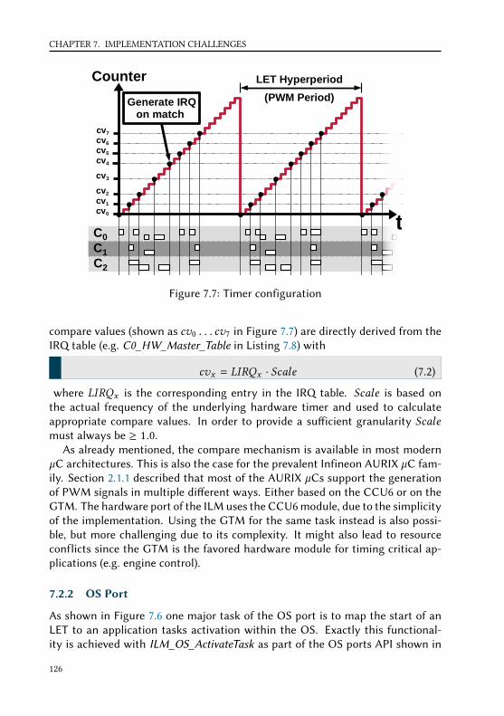
CHAPTER 7. IMPLEMENTATION CHALLENGES
C0C1C2
cv0
cv1
cv2
cv3
cv4
cv5
cv6
cv7
(PWM Period)
LET Hyperperiod Counter
t
Generate IRQon match
Figure 7.7: Timer configuration
compare values (shown as cv0 . . . cv7 in Figure 7.7) are directly derived from theIRQ table (e.g. C0_HW_Master_Table in Listing 7.8) with
cvx = LIRQx · Scale (7.2)
where LIRQx is the corresponding entry in the IRQ table. Scale is based onthe actual frequency of the underlying hardware timer and used to calculateappropriate compare values. In order to provide a suicient granularity Scalemust always be ≥ 1.0.
As already mentioned, the compare mechanism is available in most modernµC architectures. This is also the case for the prevalent Infineon AURIX µC fam-ily. Section 2.1.1 described that most of the AURIX µCs support the generationof PWM signals in multiple dierent ways. Either based on the CCU6 or on theGTM. The hardware port of the ILM uses the CCU6 module, due to the simplicityof the implementation. Using the GTM for the same task instead is also possi-ble, but more challenging due to its complexity. It might also lead to resourceconflicts since the GTM is the favored hardware module for timing critical ap-plications (e.g. engine control).
7.2.2 OS Port
As shown in Figure 7.6 one major task of the OS port is to map the start of anLET to an application tasks activation within the OS. Exactly this functional-ity is achieved with ILM_OS_ActivateTask as part of the OS ports API shown in
126

7.2. LET IMPLEMENTATION WITH ZERO-TIME COMMUNICATION
Listing 7.11: OS port API
1 /* Task activation and state check */2 void ILM_OS_ActivateTask (ILM_TASKS_T TaskId );3 void ILM_OS_SetEvent (ILM_TASKS_T TaskId , void *pEvent );4 uint32 ILM_OS_CheckTaskState (ILM_TASKS_T TaskId );56 /* Synchronous task context reentry */7 void ILM_OS_Set_BarrierMask(ILM_COREMASK_T CoreMask ); /* Only on master core */8 void ILM_OS_SyncCores (void); /* On all cores */
Listing 7.12: Master core IRQ handlerbased on ERIKA OS
1 ISR2(ILM_OS_Isr)2 3 #if ILM_USE_HOOK_START_IRQ > 04 ILM_HOOK_START_IRQ ();5 #endif6 if(ILM_HW_Isr_Master () == 1)7 8 ILM_Handler ();9 ILM_OS_SyncCores ();
10 11 #if ILM_USE_HOOK_STOP_IRQ > 012 ILM_HOOK_STOP_IRQ ();13 #endif14
Listing 7.13: Slave core IRQ handlerbased on ERIKA OS
1 ISR2(ILM_OS_Isr)2 3 #if ILM_USE_HOOK_START_IRQ > 04 ILM_HOOK_START_IRQ ();5 #endif6 ILM_HW_Isr_Slave(EE_CURRENTCPU );78 ILM_Handler ();9 ILM_OS_SyncCores ();
1011 #if ILM_USE_HOOK_STOP_IRQ > 012 ILM_HOOK_STOP_IRQ ();13 #endif14
Listing 7.11. A second function called ILM_OS_SetEvent is used to resume theexecution of a task waiting for an event. This might be the case, if the controlledtask is equivalent to the previously discussed OSEK ECC tasks from Section 2.2.2and Figure 2.9. Third, the function ILM_OS_CheckTaskState is used to obtain thecurrent state of an executing OS task. If a task is running or ready to be executed,the function returns 1, otherwise 0. In general this function is used to check ifan OS task finishes its execution before the end of the corresponding LET. If theimplicit deadline is missed, a user defined hook function can be called.
We already mentioned, that the configuration of IRQ sources is usually un-der control of the operating system. As an example, Listing 7.12 and Listing 7.13show, how this is performed in an OSEK compliant OS like ERIKA OS. The ISR2macro defines the function name and registers the ISR to the OS during compila-tion. Additionally, several user-defined hook functions can be used to implementadditional tracing or other stu if needed. According to the behavior describedin Section 7.2.1, the event handling is executed on the master core condition-ally. In order to enable a synchronized reentry into the task context, a synchro-nization barrier is used aer the execution of each event handler (ILM_Handler).How such a synchronization barrier is implemented depends on the used OS aswell as the hardware capabilities. Checking the synchronization barrier is there-fore part of the used OS and must be implemented via ILM_OS_SyncCores as apart of the OS port. The configuration of this barrier must be according to thecores, which execute LET events for the corresponding LET IRQ. This step is per-formed inside ILM_HW_Isr_Master, since the bitfield used for IRQ redirectionalso represents the synchronization barrier configuration for the correspondingLET IRQ. The needed functionality for configuration must be implemented via
127

CHAPTER 7. IMPLEMENTATION CHALLENGES
Listing 7.14: Direct mapping to BCC
1 void Task_i(void)2 3 Call_t_i ();4 TerminateTask ();5
Listing 7.15: Grouped mapping to ECC
1 void Task_i(void)2 3 Call_t_i_0 ();4 WaitEvent(Event_t_i );5 ClearEvent(Event_t_i );6 Call_t_i_1 ();7 WaitEvent(Event_t_i );8 ClearEvent(Event_t_i );9 /*...*/
10 WaitEvent(Event_t_i );11 ClearEvent(Event_t_i );12 Call_t_i_n ();13 TerminateTask ();14
Listing 7.16: Grouped mapping to BCC
1 void (* LUT_t_i []) (void) = 2 Call_t_i_0 ,3 Call_t_i_1 ,4 /*...*/5 Call_t_i_n6 ;7 uint16 CNT_t_i = 0;8 uint16 N_t_i = sizeof(LUT_t_i )/ sizeof(void *);9 void Task_i(void)
10 11 LUT_t_i[CNT_t_i ]();12 CNT_t_i = (CNT_t_i + 1) % N_t_i;13 TerminateTask ();14
ILM_OS_Set_BarrierMask. In general, a synchronized return to the tasks’ contextis needed to ensure, that all tasks start their execution aer the pointer swapshave been performed. Otherwise, it would be possible that a task on one corestarts execution before the pointers of a remote task, previously executed on adierent core, has been swapped. As a result, a wrong input value would be read.
Even though the API defines the connection between ILM and OS, it is stillan open question how to perform the mapping between LET and OS tasks. Thedescribed BCC and ECC task models from Section 2.2.2 are based on the OSEKOS definition and have later been adapted for AUTOSAR OS. Regardless the fact,that both standards are directly tailored to the automotive domain, the definitionof ECC tasks also map to many other RTOSs like µC/OS-II. Since this dissertationtargets primarily automotive systems, the following task mapping solutions arebased on the capabilities of the BCC and ECC task models. The first possibleintegration is a direct mapping from LET tasks to distinct BCC tasks. This meansthat for each LET task λi an own OS task τi is used. This works for macro-LETtasks as well as the basic block based micro-LET scheduling. Each time the LEThandling starts a LET task λi , the OS port calls ILM_OS_ActivateTask in order totell the OS to schedule τi as soon as possible. Listing 7.14 shows an example forsuch direct mapping. The function call Call_t_i represents the execution of τi . Incase of a micro-LET this would correspond to Call_t_i_n and τi ,n for each basicblock.
While a direct mapping is the only possible mapping for a macro-LET, thisdiers in case of a micro-LET based system. As already mentioned in Section 6.3,micro-LET based synchronization is usually applied to basic function blocks whichhave been scheduled in container tasks before. Based on the previous systemdesign, the resulting LET tasks oen have common periods but dierent osets.Because of this, it is possible to map a set of micro-LET tasks which share the
128

7.2. LET IMPLEMENTATION WITH ZERO-TIME COMMUNICATION
same period to one single ECC OS task. An example, Listing 7.15 shows such amapping for a set ofn micro-LET tasks λi ,0 . . . λi ,n , which execute the basic blocksτi ,0 . . . τi ,n inside of a single OS task τi . With the start of the common period,the OS port uses ILM_OS_ActivateTask to put τi into its ready state. Therefore,the execution of Call_t_i_0 starts, when τi is scheduled according to its priority.When Call_t_i_0 finishes its execution, τi stalls due to the call of WaitEvent. In-ternally the τi enters the wait state, which is le when a call to ILM_OS_SetEventwith the corresponding event Event_t_i is issued. This is repeated until the ex-ecution of Call_t_i_n finishes. This way only one OS task is used for a set ofmicro-LET tasks which share the same period but use dierent osets inside thisperiod.
The previous mapping solutions have dierent drawbacks which might leadto a problem. For the direct mapping to BCC tasks, the maximum number ofOS tasks might be an upper limit, as this is fixed due to runtime complexity andmemory overhead. The grouped mapping to ECC tasks on the other hand doesnot have this problem. But in general, ECC tasks are to be avoided in automotivesetups, since the context switch overhead increase rapidly due to additional statechecking. We therefore propose a third mapping solution which maps micro-LETtasks with common periods to a single BCC task. An example for this solutionis shown in Listing 7.16. General idea is to use a block sequencing based on alookup table (LUT_t_i[]) and a counter (CNT_t_i) as table index. Each time theOS task is called, another basic block is executed based on the current countervalue. Due to the increment and a modulo operation based on the lookup tablesize (N_t_i), the created block sequence is repeated for each period. The dierentosets during a period are represented by the position inside of LUT_t_i[]. Forcomparison both Listing 7.15 and Listing 7.16, implement the same sequence ofbasic blocks. As mentioned in the beginning of this chapter, lookup based jumptables are a well-known technique and oen used. It is therefore not surprising,that most modern CPU architecture provide single-cycle operations to load ajump address from a table directly to the processors program counter register.This results in a very low overhead of only a few processor cycles to load thejump address and increment the counter value.
7.2.3 Memory usage
In contrast to a system without LET, additional memory is needed for controlstructures and multiple value buers. If we apply a simple double buering, thedouble amount of memory is needed for global variables. Additionally, doublebuer control structs with read and write pointers for indirection are needed.As mentioned before, we assume that a publisher subscriber paradigm is usedand therefore values are only wrien by a single task. The global data wrien by
129

CHAPTER 7. IMPLEMENTATION CHALLENGES
Listing 7.17: Memory setup on publisher
1 /* Output of T10 on C0 */2 typedef struct 3 uint32 a;4 /*5 * Contains data which is6 * written by T10 on C07 */8 uint32 y;9 uint32 z;
10 OUT_C0_T10_T;111213 /* Buffer definition for T10 on C0 */14 OUT_C0_T10_T OUT_C0_T10 [2];151617 /*18 * Read/Write pointer control struct19 * initialized with buffer entries20 */21 ILM_DATA_OUT_T OUT_C0_T10_CS = 22 .Read = (void *)& OUT_C0_T10 [0];23 .Write = (void *)& OUT_C0_T10 [1];24 ;
Listing 7.18: Memory setup on subscriber
1 /* Task local pointer backup for T20 on C1*/2 typedef struct 3 OUT_C0_T10_T * input_C0_T10;4 /*...*/5 IN_C1_T20_T;6 IN_C1_T20_T IN_C1_T20_local;7 /* Pointer backup list for T20 on C1*/8 const ILM_DATA_IN_T IN_C1_T20_L [] = 9 .pIn = &OUT_C0_T10_CS ,
10 .pLC = &IN_C1_T20_local.input_C0_T10 ,11 /*...*/12 ;13 /* Task local pointer backup for T20 on C2*/14 typedef struct 15 OUT_C0_T10_T * input_C0_T10;16 /*...*/17 IN_C2_T20_T;18 IN_C2_T20_T IN_C2_T20_local;19 /* Pointer backup list for T20 on C2*/20 const ILM_DATA_IN_T IN_C2_T20_L [] = 21 .pIn = &OUT_C0_T10_CS ,22 .pLC = &IN_C2_T20_local.input_C0_T10 ,23 /*...*/24 ;
a single task can therefore be packed with a struct. Such an example is shownin Listing 7.17, where OUT_C0_T10_T represents a struct containing the globaldata wrien by τ10 onC0. An array of this type with two entries (OUT_C0_T10[2])then acts as the actual double buer for all global values wrien by τ10. In or-der to perform the needed indirection for read and write accesses, an additionalcontrol struct OUT_C0_T10_CS is used. At the end of the corresponding LET,OUT_C0_T10_CS.Read and OUT_C0_T10_CS.Write get swapped. Therefore, thepayload field in Listing 7.9 references structs of type ILM_DATA_OUT_T for eachILM_EVENT_PSWAP.
Inside each subscribing task, a struct is needed to store read pointers of allrelevant publishing tasks. In Listing 7.18 the corresponding variables for pointerbackups are IN_C1_T20_local onC1 and IN_C2_T20_local onC2. In order to knowwhich pointer should be saved during LET task activation, the ILM provides alist struct, called ILM_DATA_IN_T, used during LET event handling. Inside thestruct a reference to the corresponding publisher output (.pIN) and the localbackup (.pLC) is stored for each input. ForC1 andC2 the resulting lists are givenas IN_C1_T20_0_L and IN_C2_T20_0_L in Listing 7.18. References to those listsare then stored in the payload fields of the core local LET event table for eachILM_EVENT_TACT event.
Figure 7.8 shows the resulting mapping of the previously described manage-ment variables and buers. The pointer control struct and the correspondingbuer must be located in a globally available memory, since it is accessed bypublisher and subscribers. Additionally, the control struct is modified by the LETevent handler of C0. The local read pointer backup and the copy lists, processedby the cores of the subscribing tasks, can be located close coupled to the corre-sponding cores. Read or write accesses to either the backup stucts or the copy
130

7.2. LET IMPLEMENTATION WITH ZERO-TIME COMMUNICATION
Global Memory
C0
OUT_C0_T10[1]
OUT_C0_T10[0]
OUT_C0_T10_CS
.Write
.Read
C0_Task_10
C1IN_C1_T20_local
C2 IN_C2_T20_local
Write Read Backup Swap
IN_C1_T20_L[]
IN_C2_T20_L[]
During LET EventDuring Task Execution
Figure 7.8: Memory location of double buer and control structs
lists are only performed by the corresponding tasks or the LET event handlinglocated on the core.
Comparing the local backup with the components located in the global mem-ory shows an important dierence regarding CPUs with caches. Even thoughthe pointer backup and copy lists can also be stored in a global memory, a mech-anism preserving cache coherency in not necessarily needed since the variablesare only accessed by one core. In case of the control structs and buers located inthe global memory this is dierent. Without a coherency mechanism it could notbe ensured that the subscribed tasks always read the correct values if cachingis used by the CPUs. As a result, the cores of the subscribing tasks would needto flush their caches during each task activation. It is therefore highly recom-mended to use caching only, if the CPU implements a coherency mechanism.Otherwise, a performance loss is the case.
If we again take a look at the most prevalent AURIX µC family we realize, thatthe previous statement regarding the cache coherency does not hold. We alreadymentioned in Section 2.1.1 that TriCore CPU architecture used by the AURIXdoes not implement any kind of coherency mechanism. Therefore, the globalmemory implemented with the AURIX’s LMU can not be used to store pointercontrol structs and buers. Since the core local scratch pad RAMs (DSPR) canbe configured to be accessible from remote cores, we recommend using those in-stead. In order to provide fast access for publishing tasks, pointer control structsand buers should always be located in the DSPR of the core, executing the cor-responding publishing task.
131

CHAPTER 7. IMPLEMENTATION CHALLENGES
132

CHAPTER8
Evaluation
"We were first-class troublemakers. We did unconventionalthings in unconventional ways and still got valuable results.
Thus management had to tolerate us and let us alone a lotof the time."
- Richard Wesley Hamming
In order to prove the proposed mechanisms, we evaluate both approaches basedon exemplary implementations, executed on existing hardware as a part of well-known RTOSs. Primary focus when designing scheduler or OS modifications isthe introduced runtime and memory overhead. An evaluation regarding over-head is therefore self-evidently. Since the proposed mechanism has been devel-oped according to dierent requirements, it makes sense to evaluate dierentaspects. In case of the proposed SPS based budget scheduling, the suicienttemporal isolation with improved response times is the most important feature.Therefore, we evaluate actual task response times for the dierent schedulingmechanisms and compare them to previous results of an actual RTA. This diersfor the evaluation of the LET implementation. Since the actual scheduling staysthe same and is independent of the LET implementation, it doesn’t make senseto include this. Instead, evaluating the resulting sensitivity to additional higherpriority load for an LET based system provides more interesting results since itprovides an overview of the applicability of the LET paradigm. The evaluationresults presented in this chapter are based on [23, 24, 25, 26, 27, 28].
133

CHAPTER 8. EVALUATION
8.1 SPS based budget scheduling
The analysis of the SPS based budget scheduling consists of two major parts.First an evaluation of the RTA and second, an evaluation of measured responsetimes from an implementation. As an execution framework for the RTA pyCPAin combination with the PyPy interpreter and a multi-threaded execution on 4cores Intel Xeon [email protected] is used. The implementation of the proposedmechanisms are executed on an ARM926EJ-S based development board with anNXP LPC3250 on top of the existing hypervisor µC/OS-MMU.
8.1.1 WCRT Analysis
In order to evaluate response time of the SPS based budget scheduling, a set ofsynthetic task-sets is used and compared against the calculated response timesof a TDMA based scheduling. The evaluation is based on the pyCPA frameworkand therefore mainly wrien in Python. For task-set generation we used a scriptfrom Paul Emberson [42], which is based on Roger Staords Random Vectors withfixed Sum algorithm [100] and conveniently available as a Python implementa-tion. The provided script generates a set of periodic tasks for a given utilization,with randomly distributed periods over a defined range. In order to achieve amore arbitrary task behavior, an additional random jier, minimum distance andrelative deadline is generated for each task. The priorities are assigned based onRMS, according to the task periods.
For the analysis evaluation two dierent scenarios are used, both with an over-all number of four partitions, where one partition is reserved for the hypervisoritself. In a real implementation, this reserved partition is oen used for house-keeping and can be characterized for the analysis with a single task. For evalua-tion, the utilization of the hypervisor partition is fixed to 4%. The three remainingapplication partitions got each a synthetic task-set assigned with a random uti-lization between 15% . . . 20%, generated by the previously mentioned script fromEmberson et al. For each task inside a partition an activation jier was assignedrandomly limited to 50% of the tasks period. Same was done for deadlines, whichare defined randomly at generation between 75% . . . 125% of the correspondingtasks period.
For the first scenario, 60 setups has been generated with a varying numberof tasks from two to four inside the application partitions. Figure 8.1 shows thesteps, performed during evaluation. For each setup the optimization algorithmfrom Section 4.5.1 is executed with a step granularity of ∆ = 1µs . The calculatedslack is then distributed equally based on (4.28). The optimization provides a setof possible TDMA configurations for the hypervisor scheduling. From this set allconfigurations with 0%, 5%, 10%, 15% or 20% slack are used for further evaluation.
134
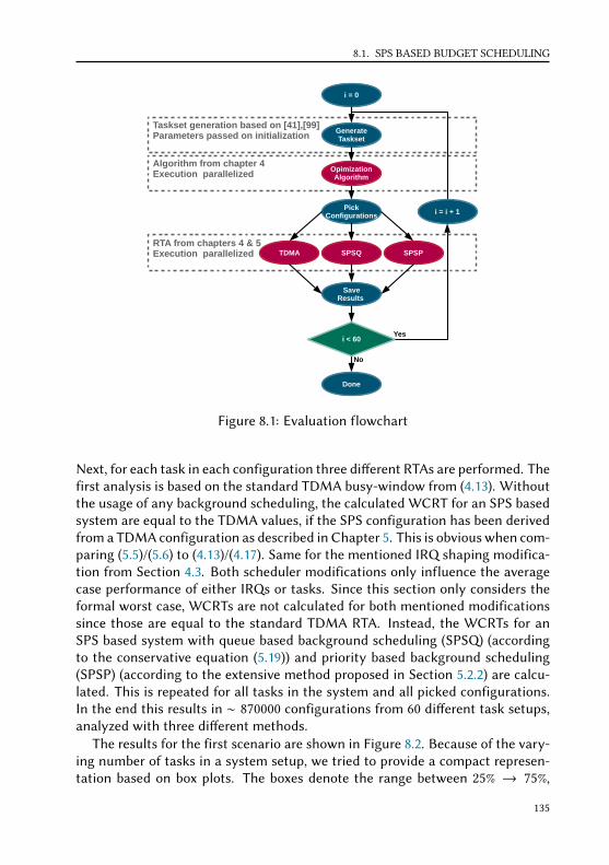
8.1. SPS BASED BUDGET SCHEDULING
Taskset generation based on [41],[99]Parameters passed on initialization
Algorithm from chapter 4Execution parallelized
RTA from chapters 4 & 5Execution parallelized
GenerateTaskset
SaveResults
PickConfigurations
i = 0
i < 60
No
Yes
i = i + 1
OpimizationAlgorithm
SPSQTDMA SPSP
Done
Figure 8.1: Evaluation flowchart
Next, for each task in each configuration three dierent RTAs are performed. Thefirst analysis is based on the standard TDMA busy-window from (4.13). Withoutthe usage of any background scheduling, the calculated WCRT for an SPS basedsystem are equal to the TDMA values, if the SPS configuration has been derivedfrom a TDMA configuration as described in Chapter 5. This is obvious when com-paring (5.5)/(5.6) to (4.13)/(4.17). Same for the mentioned IRQ shaping modifica-tion from Section 4.3. Both scheduler modifications only influence the averagecase performance of either IRQs or tasks. Since this section only considers theformal worst case, WCRTs are not calculated for both mentioned modificationssince those are equal to the standard TDMA RTA. Instead, the WCRTs for anSPS based system with queue based background scheduling (SPSQ) (accordingto the conservative equation (5.19)) and priority based background scheduling(SPSP) (according to the extensive method proposed in Section 5.2.2) are calcu-lated. This is repeated for all tasks in the system and all picked configurations.In the end this results in ∼ 870000 configurations from 60 dierent task setups,analyzed with three dierent methods.
The results for the first scenario are shown in Figure 8.2. Because of the vary-ing number of tasks in a system setup, we tried to provide a compact represen-tation based on box plots. The boxes denote the range between 25% → 75%,
135

CHAPTER 8. EVALUATION
SPSQ SPSP SPSQ SPSP SPSQ SPSP SPSQ SPSP SPSQ SPSP
0% 5% 10% 15% 20%
0.2
0.4
0.6
0.8
1.0
No
rma
lized
WC
RT
(SP
S/
TD
MA
)
Figure 8.2: Merged representation of calculated SPS based WCRTs relative toTDMA
the black dot indicates the average and the red bar the median of all calculatedvalues. In general for each task WCRT a normalized value relative to the corre-sponding TDMA based WCRT for the same configuration is calculated. A valueequal 1.0 in this plot means, that the SPS based budged scheduling for the con-sidered task and the current configuration does not provide a beer WCRT com-pared to TDMA. Values < 1.0 therefore represent an improvement compared toTDMA. This way it is possible to compare the calculated WCRTs for all task ina single graph, even though the number of tasks may change in dierent con-figurations. As an example, the box plot Q from SPS0 contains the WCRTs of allgenerated task under SPS based budget scheduling with a background schedul-ing implementing queues for all evaluated configurations with 0% slack in thecorresponding TDMA schedule. In contrast to this, P from SPS0 contains theWCRTs from the exact same configurations with 0% slack, but with a prioritybased background scheduling, assinging a disting background priority to eachpartition. The collected results show that for all calculated WCRTs both SPSbased methods with background scheduling provide at least the same WCRTbound, but oen a way beer value compared to TDMA. None of the calculatedWCRTs for both methods were greater than the corresponding TDMA WCRTconsidering the same configuration.
As you can see, it is more likely to achieve beer WCRTs compared to the stan-dard TDMA scheduling if the slack inside the system increases. Also, prioritizingsingle partitions during background scheduling may also improve the WCRTs ofthe considered partition. When considering the worst-case behavior, this doesnot have any eect to the WCRTs of the remaining partitions with smaller priori-ties. Reason for this is, that the analysis of a queue based background schedulingalways assumes the maxmimum blocking from other partitions, which is equalto the lowest priority in a priority based scheduling. In case of actual measuredresponse times, this is dierent and will be shown in Section 8.1.2. The resultsalso show that for some tasks and some configurations a SPS based system does
136

8.1. SPS BASED BUDGET SCHEDULING
not provide beer WCRTs, since all box plots reach up to 1.0. This is due to thefact that the box plots include the results for all tasks of each generated setup.Therefore, also tasks are included which would never see any benefit, based onits task parameters e.g. based on its partition internal priority or its period.
In order to explain this further more, a second evaluation is performed. Againa parameter setup with 60 task-sets as well as identical generation parametersfor utilization, period, priorities, jier and deadlines is used. Also, a distinct hy-pervisor partition is included in each task-set, leaving room for three additionalapplication partitions. Again the same evaluation flow as described in Figure 8.1is used. The major dierence is that the number of possible tasks is fixed to fourfor each application task-set. This way it is possible to show the dierent cal-culated response times for each task individually. Like before only a subset ofall possible configurations with either 0%, 5%, 10%, 15% or 20% slack are taken forfurther calculations leading to ∼ 990000 configurations. Again, for each task ineach configuration a RTA is performed. The results for queue based and prioritybased background scheduling relative to TDMA are shown in Figure 8.3. Everytask in the system is listed individually and therefore the influence of a prioritybased background scheduling can be seen beer compared to Figure 8.2. In gen-eral the tasks are described as τp,i with p indicating the partition and i a taskinside this partition. The priority inside partitions is ordered in reverse, resultingin i = 1 as highest task priority. For the priority based background scheduling,we define partition p = 4 to be the highest priority and repeat this for all remain-ing partitions in descending order. This results in the lowest background priorityfor the hypervisor partition p = 1 and its single task τ1,1.
The WCRT distribution is shown for all seings from 0% up to 20% slack inFigure 8.3a. . . 8.3e. First, a task with a high priority inside a partition might seemuch lesser improvement, especially for configurations where the amount ofslack is small. Important is at this point the amount of background schedulingincluded during the busy-window of the task under analysis. A high prioritytask inside a partition is scheduled first, when the corresponding partition isdispatched by the hypervisor. This means, that the busy-window of such a taskmight not contain any background scheduling, resulting in the same WCRT com-pared to TDMA. In contrast to this, a lower priority task inside a partition gen-erally sees more interference due higher priority inside the partition. This leadsto a longer busy-window which therefore might contain background scheduling.Second, the benefit of a priority based background scheduling can be seen fortasks inside partitions 4 and 3. Comparing queue based (Q) and priority based(P) background scheduling shows a significant improvement for tasks in parti-tions with a higher background priority. This is especially the case for configura-tions with more slack (e.g. Figure 8.3e and 8.3d). Here the tasks inside a partition(τ4,1 . . . τ4,4) with a high background priority achieve significant beer calculated
137

CHAPTER 8. EVALUATION
Q P Q P Q P Q P Q P Q P Q P Q P Q P Q P Q P Q P Q Pτ1,1 τ2,1 τ2,2 τ2,3 τ2,4 τ3,1 τ3,2 τ3,3 τ3,4 τ4,1 τ4,2 τ4,3 τ4,4
0.20.30.40.50.60.70.80.91.0
Nor
mal
ized
WC
RT
(SP
S/
TD
MA
)
(a) Distribution for 0% slack
Q P Q P Q P Q P Q P Q P Q P Q P Q P Q P Q P Q P Q Pτ1,1 τ2,1 τ2,2 τ2,3 τ2,4 τ3,1 τ3,2 τ3,3 τ3,4 τ4,1 τ4,2 τ4,3 τ4,4
0.10.20.30.40.50.60.70.80.91.0
Nor
mal
ized
WC
RT
(SP
S/
TD
MA
)
(b) Distribution for 5% slack
Q P Q P Q P Q P Q P Q P Q P Q P Q P Q P Q P Q P Q Pτ1,1 τ2,1 τ2,2 τ2,3 τ2,4 τ3,1 τ3,2 τ3,3 τ3,4 τ4,1 τ4,2 τ4,3 τ4,4
0.10.20.30.40.50.60.70.80.91.0
Nor
mal
ized
WC
RT
(SP
S/
TD
MA
)
(c) Distribution for 10% slack
Q P Q P Q P Q P Q P Q P Q P Q P Q P Q P Q P Q P Q Pτ1,1 τ2,1 τ2,2 τ2,3 τ2,4 τ3,1 τ3,2 τ3,3 τ3,4 τ4,1 τ4,2 τ4,3 τ4,4
0.10.20.30.40.50.60.70.80.91.0
Nor
mal
ized
WC
RT
(SP
S/
TD
MA
)
(d) Distribution for 15% slack
Q P Q P Q P Q P Q P Q P Q P Q P Q P Q P Q P Q P Q Pτ1,1 τ2,1 τ2,2 τ2,3 τ2,4 τ3,1 τ3,2 τ3,3 τ3,4 τ4,1 τ4,2 τ4,3 τ4,4
0.10.20.30.40.50.60.70.80.91.0
Nor
mal
ized
WC
RT
(SP
S/
TD
MA
)
(e) Distribution for 20% slack
Figure 8.3: Comparison of queue and priority based background scheduling
138

8.1. SPS BASED BUDGET SCHEDULING
WCRTs for all tested configurations with 20% slack.The two previously described scenarios resulted in ∼ 1860000 dierent con-
figurations. Evaluating the WCRTs for all tasks of those configurations took ∼ 7hours on an Intel Xeon [email protected]. In general, analyzing the runtime offixed-point iterations is always a challenge. The busy-window itself must be it-erated several times until a fix-point is reached. In case of the multiple eventbusy-windows the entire iteration might be repeated several times for a numberof events. Both, the number of iteration and the number of considered events,heavily depend on the task-set. Since all the proposed mechanisms are con-structed based on the busy-window technique, this dependency can be seen inall methods. The cycle optimization is basically a busy-window based TDMARTA performed several times with dierent parameters. The number of RTAs tobe performed is directly related to the theoretical upper bound from (4.27) andthe used stepsize ∆.
Since all values are identical in case of the described SPS configuration, theRTA of an SPS based system without background scheduling does not only pro-vide the same WCRT, it also takes the same amount of time. The RTA of a systemwith queue based background scheduling based on (5.19) also results in a moreor less equal runtime complexity compared to a TDMA RTA. At least for the com-plex calculation method from Section 5.2.2, a comparison is possible. One mightsee, that based on the dierent orders from (5.17), the entire busy-window iter-ation is executed for each possible partition order. Therefore, the analysis run-time for such a system scales based on the number of possible partition ordersY , which is given as:
Y = (|ΓHYP | − 1)! (8.1)
Due to this fact, the complex calculation method takes much more time forcomputation. Nevertheless, only the complex analysis method for SPS basedsystems is able to handle dierent types of background scheduling. Instead, thesimplified method from (5.19) can only handle queue based systems. It is stilla design-time problem, which is not relevant during runtime. Also, calculatingresponse times for a single configuration is comparatively fast on modern com-puters. The following numbers in Table 8.1 are used to highlight this and showthe actual analysis runtime for a single task-set from Table 8.2, which is later usedin Section 8.1.2 for actual runtime measurements. The optimization is performedon all possible time cycle sizes with a stepsize of 1µs . The actual RTAs are thenperformed only on a single configuration with the maximum amount of absoluteslack inside the TDMA schedule. All measurements include the overhead of theused pyCPA implementation.
139

CHAPTER 8. EVALUATION
Optimization ∼ 5200ms
TDMA/SPS ∼ 50ms
SPSQ ∼ 55ms
SPSP ∼ 65ms
Table 8.1: Analysis runtime in [ms]
8.1.2 Response time measurements
For evaluation, all proposed mechanisms are tested in an implementation on topof an existing hypervisor architecture. This includes the proposed IRQ shap-ing as well as the SPS based budget scheduling with and without backgroundscheduling (queue and priority based). The modified hypervisor setup is basedon µC/OS-MMU [41] with µC/OS-II [68] as guest OS inside partitions. WhileµC/OS-II does not directly implement an OSEK or POSIX API, it provides a sim-ple SPP scheduling with up to 256 priorities, where 0 denotes the highest priorityin the system (or partition in this case). In order to implement the CB_Idle(p)callback, a service call to the hypervisor is added inside the partitions via a hookfunction of the µC/OS-II idle-task. This way the service call is always invokedwhen a partition has nothing to do, which is exactly the behavior explained inSection 7.1.3. Also, theCB_Resume(p) callback is invoked for each partition-leveltask activation as well as for IRQs to achieve the desired behavior.
The applications inside the partitions are simulated by a generic task-set im-plementation which allows a simple execution time simulation. The task param-eters are shown in Table 8.1 and represent a simple PJ-model with period andjier. Each task activation is generated with a timer according to the correspond-ing period P and pseudo random jier within the range of J . The execution timeC is then simulated with a processor specific inline assembly. If a task misses itsdeadline D, a service call to the hypervisor core is generated and saved for laterevaluation. The evaluation setup from Table 8.2 again consists out of four parti-tions, where one partition is reserved for the hypervisor itself. Again this leavesroom for three application partitions with four tasks each. Since the hypervisorpartition is used for housekeeping like internal garbage collection or serial de-bug output, the assigned single task in Table 8.1 is only artificial and used duringthe time cycle optimization. Speaking of this, the time cycle optimization re-sults in a timecylce lengthTTDMA and timescycle slackTS . All times are given inmilliseconds.
TTDMA = 48.3, TS = 14.3
Distributing the slack equally according to (4.28) and adding this to the minimaltimeslot sizes T1,min . . .T4,min leads to:
140

8.1. SPS BASED BUDGET SCHEDULING
Hypervisor (T1 = 2.8) Partition 1 (T2 = 11.4)Prio P J C D Prio P J C D1 100 0 4 100 1 50 5 2 50
2 100 5 4 1003 200 5 6 1004 400 5 10 200
Partition 2 (T3 = 18.0) Partition 3 (T4 = 16.1)Prio P J C D Prio P J C D1 50 5 3 50 1 100 5 4 752 75 5 6 75 2 150 5 6 853 150 5 7 150 3 200 5 8 1504 175 5 10 175 4 250 5 12 175
Table 8.2: Evaluation task-set, all times are given in [ms]
T1,min =2.0 T2,min =8.0 T3,min =12.7 T4,min =11.3T1,S =0.8 T2,S =3.4 T3,S =5.3 T4,S =4.8T1 =2.8 T2 =11.4 T3 =18.0 T4 =16.1
TTDMA =T1 +T3 +T3 +T4 = 48.3
In order to evaluate the proposed runtime mechanisms, the task-set from Ta-ble 8.2 is executed based on the previously derived configuration for the followinghypervisor setups:
1. TDMA: Default TDMA scheduling used as baseline
2. TDMAS: TDMA + IRQ shaping
3. SPS: SPS w.o. background scheduling
4. SPSQ: SPS w. queue based background scheduling
5. SPSP: SPS w. priority based background scheduling
Since especially the IRQ shaping, but also the SPS based budget scheduling, tar-get to improve the response times of IRQs, those need to be evaluated as well. Inorder to test this, an exponentially distributed IRQ paern, generated by one ofthe processor’s hardware timers, is used. The distributed IRQ paern is charac-terized by the mean interarrival rate given as:
λ = U /CBH (8.2)
141
CHAPTER 8. EVALUATION
For each system setup 14000 IRQs with a mean loadU = 30% and CBH = 500µsare generated. The appropriate BH is located in partition 1 (T2). Therefore, themonitors of the remaining partitions during the TDMAS test get configured ac-cording to Section 4.3. All other tests use the exact same IRQ paern but withoutany IRQ shaping, therefore no monitoring needs to be configured for those tests.
Before we focus on the actual response times, we first consider the dierentIRQ handling types. As a kind reminder of Chapter 4, an IRQ is markt as Directhandled if it occurs during execution of the corresponding partition. If an IRQoccurs during the execution of a foreign partition, it is stored and handled aer-ward when the corresponding partition is executed again. In that case an IRQ ismarked as Delayed. The IRQ shaping provides a third option, which handles anIRQ Interposed and preempts the currently scheduled partition. Figure 8.4 showsthe distribution of this dierent IRQ handling methods as histograms over themeasured response time. To clarify this, Figure 8.4a show that in case of a stan-dard TDMA scheduling all Direct IRQs have a short response time. In contrastto this, the response times of Delayed IRQs are more or less equally distributedacross a wider response time range. When using IRQ shaping this distributionchanges, as shown in Figure 8.4b. All Interposed IRQs get handled immediatelyinstead of Delayed and show therefore a short response time in Figure 8.4b. Asthe absolute number of delayed IRQs decreases, the relative probability for De-layed IRQs shis towards the le.
For the SPS based scheduling mechanisms the results are shown in Figure 8.4c,8.4d and 8.4e. Even though an Interposed IRQ handling is not available for thisscheduling mechanisms, it performs similar, since even Delayed IRQs get mostlyhandled within a short time. Primary reason for this is the SPS based mech-anisms, which adapts the budget provisioning to the actual usage. Comparedto a standard TDMA scheduling this leads to an adaptive usage of the availablebudget and therefore shorter response times for Delayed handled IRQs.
142

8.1. SPS BASED BUDGET SCHEDULING
0 5 10 15 20
Response time in [ms]
0
20
40
60
80
100
Pro
ba
bili
tyin
[%]
Direct
Delayed
Interposed
(a) TDMA
0 5 10 15 20
Response time in [ms]
0
20
40
60
80
100
Pro
ba
bili
tyin
[%]
Direct
Delayed
Interposed
(b) TDMAS
0 5 10 15 20
Response time in [ms]
0
20
40
60
80
100
Pro
ba
bili
tyin
[%]
Direct
Delayed
Interposed
(c) SPS
0 5 10 15 20
Response time in [ms]
0
20
40
60
80
100P
rob
ab
ility
in[%
]Direct
Delayed
Interposed
(d) SPSQ
0 5 10 15 20
Response time in [ms]
0
20
40
60
80
100
Pro
ba
bili
tyin
[%]
Direct
Delayed
Interposed
(e) SPSP
Figure 8.4: Response time distribution for dierent IRQ handling paths
143

CHAPTER 8. EVALUATION
Next we take a look at the actual response times of both IRQs and tasks, col-lected for the dierent scheduling techniques. During all tests no task deadlinehas been violated. As already mentioned in Section 7.1.3, the provided implemen-tation is based on multiple queues and the insertion method defines the actualbackground scheduling. In order to provide measurements also for priority basedbackground scheduling, we prioritized Partition 1 over all other partitions. Insidethe implementation this is a simple task, as the queues are based on double linkedlists. Therefore, adding a partition at the head instead of the tail corresponds toadding it with the “highest” priority to the background scheduling. The resultspresented in Figure 8.5 and 8.6 only show the measurements from Partition 1 inorder to highlight the dierence between queue based and priority based back-ground scheduling.
The results in Figure 8.5 show the measured response times as box plots. Likebefore, the boxes denote the range between 25%→ 75%, the black dot indicatesthe average and the red bar the median of all measured values. Additionally,the ∇ symbols indicate the calculated WCRTs. Comparing the standard TDMAscheduling to a scheduling with IRQ shaping (TDMAS) shows for all tasks, thatthe improvement of IRQs is achieved at the expense of tasks. Even though theSPS without any background scheduling provides the same worst-case, the av-erage case improvement compared to TDMA can directly be seen for both IRQsand tasks. The more flexible SPS scheduling provides much beer response timesto higher priority tasks or IRQs which get processed right aer a partition wasdispatched. With background scheduling, this is improved further more also forlower task priorities. While the worst-case for tasks with higher priority insidethe partition is more or less the same compared to TDMA for both backgroundscheduling techniques, it significantly improves for lower task priorities. This isdue to the already explained reason that higher priority tasks may not benefitfrom background scheduling during the RTA. Regarding the actual measure-ments, an improvement is clearly visible, even though the dierence betweenSPSQ and SPSP is only minor for the used task-set. In order to show this im-provement further more, Figure 8.6 shows the response time histograms for thefour considered tasks of Partition 1 and the corresponding IRQ. Again a shitowards the shorter response times is clearly visible for the SPS based schedul-ing mechanisms. Important is at this point, that this is achieved while preserv-ing a comparable improvement like TDMAS also for IRQs compared to standardTDMA. Also, keep in mind that the mechanisms providing this improvement,still ensures a suicient temporal isolation according to Definition 4.3.
144
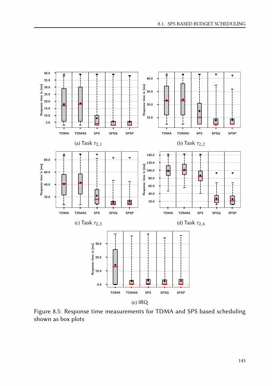
8.1. SPS BASED BUDGET SCHEDULING
TDMA TDMAS SPS SPSQ SPSP
5.0
10.0
15.0
20.0
25.0
30.0
35.0
40.0
Res
po
nse
tim
ein
[ms]
(a) Task τ2,1
TDMA TDMAS SPS SPSQ SPSP
10.0
20.0
30.0
40.0
Res
po
nse
tim
ein
[ms]
(b) Task τ2,2
TDMA TDMAS SPS SPSQ SPSP
20.0
40.0
60.0
80.0
Res
po
nse
tim
ein
[ms]
(c) Task τ2,3
TDMA TDMAS SPS SPSQ SPSP
20.0
40.0
60.0
80.0
100.0
120.0
140.0
Res
po
nse
tim
ein
[ms]
(d) Task τ2,4
TDMA TDMAS SPS SPSQ SPSP
0.0
10.0
20.0
30.0
Res
po
nse
tim
ein
[ms]
(e) IRQ
Figure 8.5: Response time measurements for TDMA and SPS based schedulingshown as box plots
145

CHAPTER 8. EVALUATION
5 10 15 20 25 30 35 40
Response time in [ms]
0
10
20
30
40
50
60
70
Pro
ba
bili
tyin
[%]
TDMA
TDMAS
SPS
SPSQ
SPSP
(a) Task τ2,1
5 10 15 20 25 30 35 40
Response time in [ms]
0
10
20
30
40
50
60
Pro
ba
bili
tyin
[%]
TDMA
TDMAS
SPS
SPSQ
SPSP
(b) Task τ2,2
10 20 30 40 50 60 70 80 90
Response time in [ms]
0
10
20
30
40
50
60
70
Pro
ba
bili
tyin
[%]
TDMA
TDMAS
SPS
SPSQ
SPSP
(c) Task τ2,3
20 40 60 80 100 120 140
Response time in [ms]
0
10
20
30
40
Pro
ba
bili
tyin
[%]
TDMA
TDMAS
SPS
SPSQ
SPSP
(d) Task τ2,4
0 5 10 15 20 25 30 35
Response time in [ms]
0
10
20
30
40
50
60
70
Pro
ba
bili
tyin
[%]
TDMA
TDMAS
SPS
SPSQ
SPSP
(e) IRQ
Figure 8.6: Response time measurements for TDMA and SPS based schedulingshown as histograms
146

8.1. SPS BASED BUDGET SCHEDULING
8.1.3 Runtime and memory overhead
Table 8.3a shows a comparison of the hypervisors memory usage for three dif-ferent scheduler configurations. First the original TDMA scheduler, second theTDMA scheduler including the IRQ shaping mechanism and third the SPS basedmechanisms with budget scheduling. The original TDMA scheduler is in all ar-eas the smallest one. But keep in mind that here a commercial implementation iscompared with two academic implementations, which might have not been op-timized to the limit. While TDMAS only required a modification of the existingscheduler, is has been replaced entirely within the SPS implementation. Only theactual dispatch mechanisms have been recycled. Both modified versions show asimilar code size and memory usage. An important thing to mention is that themonitoring used for the IRQ shaping does not have a constant overhead for dif-ferent scheduling parameters. When changing the monitors trace length (storedin the data segment) as mentioned in [89], this does aect memory usage as wellas the static runtime overhead. As described in Section 4.3, the trace length de-pends on the actual amount of available slack. Therefore, the overhead wouldincrease for systems with more slack. As the SPS does not use this mechanismanymore, the memory usage and the runtime overhead are independent of theschedulers parameters.
Table 8.3b shows the WCETs of the most important parts of the SPS implemen-tation with background scheduling. As mentioned before, background schedul-ing is based on an additional queue with only a lazy implementation of a sin-gle additional background priority for evaluation. The gathered values thereforepresent the SPSQ case, which is more or less identical to the used implementa-tion during the SPSP evaluation. Since measuring WCETs is a fairly complex task,we used OTAWA [20] to derive this values based on a static assembly level codeanalysis. Without any runtime dependent loops inside the code and statementsprimarily based on switch case resulting in look up tables, this should provide asuicient estimation. The LPC3250 on the used development board is clocked at
TDMA TDMAS SPS Q/PCode 121964 124808 125548Data 381576 382576 381776
Sum 503540 507384 507324(a) Memory usage in bytes
CPU CyclesHandler Callback
Refill 3840 1555Empty 3445 2690Resume 4760 2345Idle 4885 1255
(b) WCET in cycles
Table 8.3: System overhead
147

CHAPTER 8. EVALUATION
200MHz which results in 200Cyclesµs . Therefore, 2000 cycles correspond to 10µs .
While the proposed mechanisms can be implemented with limited memory over-head as mentioned before, the actual execution time overhead still depends onthe functions of the underlying OS or RTE. As an example, the scheduler callbackfunctions use the underlying queue system which itself is based on the internalmemory management of µC/OS-MMU. In order to push an entry to one of thequeues, first the memory of the entry is allocated based on the underlying mem-ory management. This step on its own may take up to 1000 cycles, leaving lotsof room for improvement.
8.2 LET implementation with Zero-Time Communication
This section evaluates the proposed Zero-Time Communication based on the ILMimplementation. First an overview of the memory and runtime overhead is givenand second the behavior under overload is considered. The evaluation is basedon an example from Daimler RD/EIS, which represents a micro-LET based dis-tribution of application soware from an ECU of the powertrain subdomain. Asexecution platform an Infineon AURIX TC275TF@200MHz and ERIKA OS 2.7 isused. The corresponding hardware and OS port are part of the freely availableILM [7]. The entire system is compiled and optimized for speed with a gcc 4.6.4based toolchain (gcc -O2). All runtime values have been measured with a Lauter-bach Trace32 setup, including a 17-channel logic snier for calibration measure-ments via pin toggling. The evaluation is performed for the following three taskmapping mechanisms, which already have been discussed in Section 6.3.
BCC: Direct mapping to BCC
BCC+: Grouped mapping to BCC
ECC: Grouped mapping to ECC
8.2.1 Runtime and memory overhead
As discussed in Section 7.2, each LET event is connected to an IRQ generated ei-ther by the underlying timer hardware or through a redirected soware IRQ. Re-sulting from this, the discussed activation delay from Section 6.3 is given as dis-tance between the IRQs occurrence and the start of execution within the task’scontext. Table 8.4 shows the measured overhead for the three proposed integra-tion methods and Figure 8.7 visualizes the temporal sequence.
Aer occurrence of an IRQ, the hardware specific low-level handler is called.This is shown in Figure 8.7 and Table 8.4 as BR&R . In case of the used AURIXµC, BR&R is the time needed to reset IRQ flags and reconfigure the CCU6 to
148

8.2. LET IMPLEMENTATION WITH ZERO-TIME COMMUNICATION
BCC BCC+ ECCBR&R 0.9BC2CI 0.6BLET 1.4 1.5BC2CS 1.8 (0.9)BCTX 1 2BFBC 0 0.1 0
BACT 5.7 (4.8) 5.8 (4.9) 6.8 (5.9)
Table 8.4: Measured activation delayfor dierent implementations in µs
IRQ Context
C0
C1
BR&R
C2
BC2CI
BLET
BC2CS
BCTX
BFBC
BACT
Figure 8.7: Activation delay
the next compare value. Since the steps taken for the BCC, BCC+ and ECC arealways the same, the execution time does not dier between the dierent map-ping mechanisms. Aer the reconfiguration of the underlying timer hardware,a soware IRQ is forwarded to the slave cores. The time needed to forward andprocess this IRQ is given as BC2CI and equal for all three mapping mechanisms.Aer the soware IRQs have been redirected or handled, the LET event han-dling is executed. Measuring the runtime overhead for the processed LET eventsis crucial. Reason for this is the fact, that each LET IRQ might trigger multipleLET events. A simple example is the back-to-back execution of two tasks. In thiscase the first event swaps the buer of the previous task and the second eventactivates the subsequent task. The LET handling overhead BLET shown in Ta-ble 8.4 is exactly for this scenario. In case of an ECC based system, the overheadis slightly larger. An ECC based system might use the ILM_OS_SetEvent call,which are more expensive than an additional call of ILM_OS_ActivateTask. Aerthe event handling was executed, each involved core enters a synchronizationbarrier. The synchronization barrier is exited by all cores at the same time. Thismeans, that the core which has received the worst-case blocking yet and entersthe barrier last, only checks it once. In Figure 8.7 this is visualized for C2 withBC2CS representing the overhead for checking the synchronization barrier once.Again this part is independent of the used conformance class. We measured twodierent values for BC2CS , as we realized a comparatively large overhead of 1, 8µsfor the default synchronization barrier implementation of ERIKA OS. Therefore,we stripped this implementation and removed a not necessary spinlock call, re-sulting in only 0, 9µs overhead. The context switch overhead BCTX diers asexpected for both conformance classes. While the low-level context switch it-self does not take longer in case of an ECC based system, the additional eventhandling WaitEvent/ClearEvent is responsible for the additional overhead (com-pared to both BCC setups). The overhead for the function block call BFBC only
149
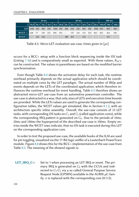
CHAPTER 8. EVALUATION
10 ms 20 ms 100 ms
λ 10,0 10,1 10,2 10,3 10,4 20,0 20,1 20,2 20,3 20,4 20,5 20,6 100,0 100,1 100,2
LET 1400 350 300 500 1200 700 400 600 250 400 500 1000 900 800 400
WCET C1 628 77 129 221 594 333 - 137 125 133 353 463 423 362 185
WCET C2 - 169 154 - - - 188 293 - 172 - - - 337 -
Table 8.5: Micro-LET evaluation use-case, times given in [µs]
occurs for a BCC+ setup with a function block sequencing inside the OS task(Listing 7.16) and is comparatively small as expected. With those values, BACTcan be constructed. The values in parentheses are based on the modified barriersynchronization.
Even though Table 8.4 shows the activation delay for each task, the runtimeoverhead primarily depends on the actual application which should be coordi-nated on multiple cores by the LET paradigm. The actual number of IRQs andevents depends on the LETs of the coordinated application, which therefore in-fluences the runtime overhead for event handling. Table 8.5 therefore shows anabstracted micro-LET use-case from an automotive powertrain controller. Theuse-case is abstracted in a way, that only sizes of LETs and execution time boundsare provided. While the LETs values are used to generate the corresponding con-figuration tables, the WCET values get simulated, like in Section 8.1.2, with anarchitecture specific inline assembly. Overall, the use-case consists of 15 LETtasks, with corresponding OS tasks onC1 andC2 (called application cores), whilethe corresponding IRQ paern is generated on C0. Due to the periods of 10ms ,20ms and 100ms the hyperperiod of the described use-case is 100ms . Empty en-tries inside the WCET rows indicate, that no OS task is executed during this LETon the corresponding application core.
In order to test the proposed use-case, the available hooks of the ILM are usedfor pin toggling, visualized via the 17-Bit logic snier of a Lauterbach PowerTracemodule. Figure 8.8 shows this for the BCC+ implementation of the use-case fromTable 8.5. The meaning of the showed signals is:
LET_IRQ_Cx : Set to 1 when processing an LET IRQ or event. The pri-mary IRQ is generated on C0 with the CCU6 and redi-rected to C1/C2 via a so called General Purpose ServiceRequest Node (GPSRN) available in the AURIX µC fam-ily. x is replaced with the corresponding core (0/1/2).
150

8.2. LET IMPLEMENTATION WITH ZERO-TIME COMMUNICATION
Figure 8.8: Execution trace of the use-case from Table 8.5
LET_yMS_Cx : Set to 1 if an LET task with period y (100/20/10) is acti-vated on application core x . Set to 0 at the end of an LETtask. As the LET tasks are sequenced back-to-back for amicro-LET system, only a small peak is visible betweenLET tasks with the same period y but dierent oset.
WCET_yMS_Cx : Set to 1 when the execution of the corresponding func-tion block inside the corresponding OS task starts. Set to0 when the block function finishes its execution. There-fore, high priority interference is indicated through a de-layed execution start or an execution that takes longerthan the corresponding WCET. Again y denotes the pe-riod and x the application core (1/2)
LET_MISS_Cx : Temporarily set to 1 if a block function is still executing,although the LET has elapsed. x is replaced with thecorresponding application core
Figure 8.8 shows the start of a hyperperiod, where LET tasks of all three peri-ods get activated aer each other. The configuration from Table 8.5 can directlybe recognized in Figure 8.8. This is possible, since the LET task sizes in the showeduse-case are equal to twice the WCET, based on a design constraint. Due to lackof high priority interference, the OS tasks start their execution directly aer theactivation of the LET task.
In order to calculate the overall overhead introduced by the LET handling,the WCET of each handler activation (CHdl ,x ) and the overall number of handleractivations per hyperperiod are necessary. Therefore, we get for each core x :
UHdl ,x =NoO f HandlerActivationsx
Hyperperiod·CHdl ,x (8.3)
The number of activations can directly be derived from the proposed LET sched-
151

CHAPTER 8. EVALUATION
ule given in Table 8.5. It results in 98 hardware IRQs onC0, where all 98 IRQs arerelevant for C1 and only 58 for C2. CHdl ,x can be measured for each core dur-ing runtime with the evaluation setup, but it can also be constructed based onFigure 8.7 and Table 8.4. Important is thatCHdl ,x includes dierent parts for dif-ferent cores. As an example, while CHdl ,0 might include overhead for the CCU6reconfiguration (given as BR&R ) it does not include the actual LET event handlingBLET as no application is executed on C0. In contrast to this, CHdl ,1 and CHdl ,2include LET event handling but don’t reconfigure the CCU6. Nevertheless, for allcores the context switch overhead must be included and also parts of the core-to-core IRQ based on the GPSRN. This results for the BCC+ implementationin:
UHdl ,0 =98
100000µs· 2.0µs ≈ 0.20%
UHdl ,1 =98
100000µs· 4.5µs ≈ 0.45%
UHdl ,2 =58
100000µs· 4.5µs ≈ 0.26%
Distributing application and IRQ generation dierently also influences the causedoverhead. Using only cores C1 and C2, with IRQ paern generation on C1, theoverhead results in:
UHdl ,0 = 0%
UHdl ,1 =98
100000µs· 7.0µs ≈ 0.70%
UHdl ,2 =58
100000µs· 4.5µs ≈ 0.26%
Important is at this point, that in this case the blocking based on the core-to-core IRQ must be considered entirely. Even though only the first part (seing theIRQ) is executed on C1, the second part on C2 (handling the IRQ) is consideredindirectly through the synchronization barrier at the end. This is not the case, ifthere is no LET event handling on the core used for IRQ generation. As an addi-tional example, moving the paern generation toC2 would increase the overheadunnecessarily, as now all IRQs are also handled onC2, even though only 58 IRQsare relevant for the local application. This would result in:
152

8.2. LET IMPLEMENTATION WITH ZERO-TIME COMMUNICATION
UHdl ,0 = 0%
UHdl ,1 =98
100000µs· 4.5µs ≈ 0.44%
UHdl ,2 =98
100000µs· 7.0µs ≈ 0.70%
Which distribution method is preferable, depends heavily on the rest of thesystem. While, combining IRQ paern generation directly with event handlingon the same core removes the need of an additional core for paern generation, itclearly increases the overhead of the LET handling. Also, LET events that are onlyrelevant for an application on another core do now cause additional interferenceto the local application. This is not the case for a setup where the IRQ paerngeneration is executed on a distinct core, as only events relevant for the localapplication are redirected to corresponding cores.
Like the runtime overhead, also the memory overhead of the proposed ILMimplementation primarily depends on the number of LET IRQs and events duringa hyperperiod. The determined memory usage is shown in Table 8.6. All resultsare based on the BCC+ implementation where the application is mapped to C1and C2. C0 is only used for IRQ paern generation. The meaning of the fivedierent memory sections is:
.text: Instructions
.bss: Uninitialized RAM variables
.data: Initialized RAM variables
.rodata: Read only variables
.global: Global RAM variables for core-to-core interactions
In order to show the important parts, the results are devided into three dierentparts. First, the LET implementation including the relevant event handling, aswell as the OS and hardware port. Second, the hook functions used for pin tog-gling and tracing and third the application including WCET simulator and theIRQ/event tables. The LET implementation primarily consists of instructions in.text and a few uninitialized system variables in .bss. In case ofC0 also the AURIXspecific hardware initialization as well as 8 bytes for bitmasks and barrier in the.global section, implementing the core-2-core synchronization, are included. Foradditional tracing via a logic snier, the hook functions implement a pin togglingresulting in additional code overhead in .text. The overhead in .data and .rodatais based on pin mapping tables which provide an abstraction layer to the usedevaluation platform.
153

CHAPTER 8. EVALUATION
.text .bss .data .rodata .globalLET implementationC0 638 62 0 0 8C1 200 17 0 0 0C2 200 17 0 0 0Hook functionsC0 166 0 184 192 0C1 146 0 0 184 0C2 158 0 0 184 0ApplicationC0 0 0 0 294 0C1 476 6 0 1724 0C2 170 6 0 952 0
Table 8.6: Memory overhead for the use-case from Table 8.5
The simulated application also generates overhead on all cores. On C0 theapplication dependent IRQ table is locate, holding 98 entries for the use-casefrom Table 8.5. According to Listing 7.8 each entry consists of a relative osetfor the timer and a bitmask for the corresponding cores. In case of the AURIXµC this can be encoded in 3 bytes (1 byte bitmask, 2 bytes oset) leading to 294bytes for 98 entries. As the table should never be changed during runtime, it islocated in the .rodata section.
OnC1 andC2 the application simulation framework generates some overheadin the .text and .bss section. Since the simulation relevant code is only neededdue to the lack of a real application, it can be neglected. Instead, the event tablesstored in .rodata are much more important. As already discussed before, theapplication reacts to 98 relayed IRQs on C1 and to 58 on C2. To each relayedIRQ multiple LET events can be assigned, leading to table entries with identicalrelative osets. Each entry uses 16 byte of memory and can encode multipleevents for the same OS task. As an example, the back-2-back activation of twoLET tasks consists of a pointer swap for the first and an activation of the secondLET task. If those LET tasks are mapped to the same OS task, both events canbe encoded with a single table entry. If the OS task diers, maybe because ofdierent periods, two separate entries are needed.
Completely missing in Table 8.6 is the additional memory overhead due todouble buering. Reason for this is the fact, that the needed data was not pro-vided with the example. In order to still be able to evaluate the needed overhead,we will have a look on the use-case from the 2017 WATERS industrial challengeused in [52, 83, 32, 34]. The system consists of 9 periodic tasks, some additional
154

8.2. LET IMPLEMENTATION WITH ZERO-TIME COMMUNICATION
IRQs and an angle synchronous cranksha task. For the sake of simplicity wewill focus only on the periodic tasks, which can be implemented as a macro-LETsystem.
Each task produces a set of outputs and takes a set of inputs. According to Sec-tion 7.2.3, the output of each task i consists of the wrien data, stored in a doublebuer (MEMOUT ,i ), and a control struct (MEMOUT _CS ,i ). The input of each taski is defined by a list of used double buers from other tasks (MEMI N _List ,i ) andlocal copies of the corresponding read pointers (MEMI N _Local ,i ). This leads to
MEMOUT ,i = 2 ·OutputDataBytesMEMOUT _CS ,i = 2 · sizeo f (pointer )BytesMEMI N _List ,i = 2 · NumO f InputData · sizeo f (pointer )Bytes
MEMI N _Local ,i = NumO f InputData · sizeo f (pointer )Bytes
with 4 bytes for the size of a pointer on the AURIX µC. In case of a ringbuerimplementation, which might store more than two values of each global datavariable, the term for MEMOUT ,i must be modified accordingly.
The periodic tasks from the 2017 WATERS challenge example write overall14256Bytes of output data. If this amount of data is stored in double buers thisleads to:
MEMOUT = 2 · 14256Bytes = 28512Bytes (8.4)
For each of the 9 tasks a distinct control struct is needed to access the corre-sponding double buer, overall this leads to:
MEMOUT _CS , = 9 · 2 · 4Bytes = 72Bytes (8.5)
The internal dependencies of the dierent tasks result in overall 61 dierentreferences to double buers which need to be processed during LET handlingand stored as task local pointer copies. This leads to:
MEMI N _List = 2 · 61 · 4Bytes = 244BytesMEMI N _Local = 61 · 4Bytes = 488Bytes
The overall memory consumption if then 29316Bytes for double buers and allother control structs. Comparing this to previous data results in a memory over-head of ∼ 106%. Judging by the numbers this overhead is dominated by thedouble buers and only a fraction of it is due to the needed control structs.Overall the memory overhead is dominated by the application specific data likeIRQ/event tables or double buers.
155

CHAPTER 8. EVALUATION
8.2.2 Overload behavior
As already mentioned, LETs can be interpreted as implicit deadlines. In case of amacro-LET system nothing changes since the deadlines introduced through LETare equal to the previous RMS based system. This is dierent in case of micro-LET as the LETs are not applied on period boundaries. As a result, micro-LETbased systems are more prone to higher priority load. In order to test this forthe proposed micro-LET system from Table 8.5 a simple method is constructedto generate high priority interference. C0 is used to generate periodic core-to-core IRQs to both application cores with dierent periods. On C1 and C2 thecorresponding ISR is executed, with a higher priority than the LET controlled OStasks but a lower than the LET event handling. The executed ISR consumes adefined value of CPU time and returns to the previous execution context. Theinterference based blocking for each application core Cx is therefore given as:
Bx ,max (∆t) = BHP ,x ,min ·
⌈∆t
Tx ,min
⌉Tx ,min represents the minimum allowed interarrival time for a higher priorityinterference of size BHP ,x ,min , under constraint that no LET is missed. BHP ,x ,minis simply the minimum of all BHP ,i on coreCx , which can be calculated accordingto Figure 6.8 via:
BHP ,i = λi − (Ci − BACT )
Table 8.7 lists all BHP ,i terms for both application cores and the three dierentintegration methods (with BACT rounded up). In case of the LET task setup onC1, λ20,3 is the LET task with the smallest available slack, for the BCC and BCC+implementation this leads to:
BACT = 5, 8µs ≈ 6µsBHP ,1,min = BHP ,20,3 = 250µs − (125µs + 6µs) = 119µs
With a given value for BHP ,x ,min , the minimum interarrival time Tx ,min can bederived. General idea is to find the smallest value forTx ,min , such that none LETis missed for a periodic interference of BHP ,x ,min with period Tx ,min on core Cx .For the given use-case this results in BHP ,1,min = 119µs every T1,min = 500µs onC1. Performing the same calculations for applicationC2 this leads to BHP ,2,min =
140µs and T2,min = 400µs . The corresponding BHP ,x ,min values are highlightedwith a bold font in Table 8.7.
Simulating the calculated higher priority load results in Figure 8.9a. The in-fluence of the higher priority load can be seen in the longer times of the WCET_*
156

8.2. LET IMPLEMENTATION WITH ZERO-TIME COMMUNICATION
10 ms 20 ms 100 ms
λ 10,0 10,1 10,2 10,3 10,4 20,0 20,1 20,2 20,3 20,4 20,5 20,6 100,0 100,1 100,2
LET 1400 350 300 500 1200 700 400 600 250 400 500 1000 900 800 400
Maximum allowed interference on C1
BCC 766 267 165 273 600 361 - 457 119 261 141 531 471 432 209
BCC+ 766 267 165 273 600 361 - 457 119 261 141 531 471 432 209
ECC 765 266 164 272 599 360 - 456 118 260 140 530 470 431 208
Maximum allowed interference on C2
BCC - 175 140 - - - 206 301 - 222 - - - 457 -
BCC+ - 175 140 - - - 206 301 - 222 - - - 457 -
ECC - 174 139 - - - 205 300 - 221 - - - 456 -
Table 8.7: Allowed higher priority interference, times given in [µs]
signals. Those signals represent in this case the response time (since higher pri-ority interference is included) of the corresponding OS task, executed within theLET boundaries. That the calculated higher priority load is at its maximum canbe seen for signal WCET_20MS_C1 at ∼ −3.060s where the execution of thecorresponding OS task is finished just before the end of the LET visualized byLET_20MS_C1. Counting the pulses on WCET_20MS_C1 shows, that the thirdexecuted OS task with period 20ms is close to miss the LET. Comparing this withTable 8.7 and 8.5 shows that the corresponding LET task is λ20,3, which matchesthe previous interference calculation. Same can be done for the execution onC2,resulting in λ10,2. Increasing BHP ,x ,min further more above the given values fromTable 8.7 on both application cores causes the system to miss LETs as shown inFigure 8.9b. The ILM detects an LET miss by checking the OS task state whenswapping read and write pointer. If the OS task hasn’t finished its execution bythat time, a user definable hook function is called. In the shown example thehook function simply toggles an output pin. Future work might include specificmechanisms like dropping activations or suspending the current execution to thenext period. At the moment this is an open research topic, since the mechanismto be toggled on an LET miss might highly depend on the actual application. Inpresent work oen only an LET miss is signalized but not handled [119]. Also,some ideas like, aborting an OS task during execution and restarting it in thenext period, might sound promising but are really hard to implement on existingsoware and hardware architectures.
157

CHAPTER 8. EVALUATION
(a)H
igh
prio
rity
load
acco
rdin
gto
Tabl
e8.
7
(b)H
igh
prio
rity
over
load
wit
hLE
Tm
isse
s
Figu
re8.
9:O
verl
oad
beha
vior
158

CHAPTER9
Conclusion
“Shut up and take my money!”
- Philip J. Fry
Within this dissertation we provided possible solutions for two known issues inmodern automotive ECUs. The primary reason for those issues is the coordina-tion of the newly available computing power in modern automotive µCs or SoCs.Even though the proposed mechanisms could not be more dierent, both targetwell-known areas inside a vehicle. Both mechanisms have been developed to tar-get the challenges defined in Section 2.3. On the one hand there is the SPS basedbudget scheduling, targeting a real-time capable hypervisor which is meant tobe part of the AUTOSAR AP. On the other hand, there is the multicore synchro-nization based on LET, targeting the issues related to the execution of legacysinglecore soware. Both mechanisms have been developed and evaluated inorder to satisfy the given requirements also given in Section 2.3.
According to Section 2.3.1 a new hypervisor scheduler should be work con-serving, with improved response times and provide suicient temporal isolationwith a low profile overhead. In order to provide a novel scheduling mechanism,several mechanisms have been described in Chapter 4 and 5. Comparing theevaluation results from Section 8.1 with the four defined requirements show theextent to which the requirements have been met by the proposed schedulingmechanisms.
With regard to improved response times, all developed scheduling mecha-
159

CHAPTER 9. CONCLUSION
nisms improve those in some way. While the IRQ shaping from Section 4.3 onlyimproves the IRQ response times, the SPS-based mechanisms from Chapter 5also improve task response times as well. Nevertheless, from the formal per-spective, only the SPS-based mechanisms with background scheduling are ableto improve not only the measured average case but also the formal worst-caseresponse times. This is a side eect of the fact, that only the SPS-based mecha-nisms with background scheduling provide the possibility of a work-conservingscheduler. While all other proposed mechanisms can not utilize idle times, dueto a fix TDMA schedule or budget enforcement, this is possible for a system withbackground scheduling. In case of suicient temporal isolation, all mechanismssatisfy Definition 4.2 formally. This is also supported by simulation results andreal world measurements in Section 8.1.
The introduced overhead by the mechanisms itself is comparatively low. Nev-ertheless, the capabilities of the underlying hardware must be taken in account,since all proposed mechanisms might introduce additional context switches. Prob-lematic is at this point not the direct overhead of the context switch, but morethe indirect overhead due to caching eects. While the used hardware for evalu-ation performs the worst due to a virtual indexed cache [28], this is dierent forarchitectures of more modern SoCs like the R-Car H3. This is due to mechanismslike an indexing based on physical addresses, address space identifiers or cachepinning.
As the results of Section 8.1 show, the SPS based mechanisms provide all a sig-nificantly beer performance compared to the standard TDMA scheduling. Evenwithout background scheduling, the SPS based mechanisms provide a much bet-ter average case behavior. If the additional computation time during analysis andthe additional code overhead for a more sophisticated background scheduling isworth investigating compared to a simple FIFO based queue, heavily depends onthe actual application.
Compared to the SPS-based scheduling, the LET implementation targets adierent problem. While the SPS-based scheduling only targets a work conserv-ing scheduling on a singlecore, a multicore synchronization is missing. The LETparadigm should be used in order to coordinate automotive soware (e.g. controlfunctionality or gateways) on mutlicore platforms. This can be performed on thebasis of a standard AUTOSAR CP application without or also on a more sophisti-cated system with virtualization (e.g. a combination of CP and AP). According tothe requirements from Section 2.3.2, the proposed solution should allow a com-parable end-to-end latency for eect chains, a minimized input jier and lowprofile overhead. If those requirements can be met entirely, depends heavily onthe executed application and the way how the LET paradigm is applied to thesoware.
We described two dierent mapping solutions discussed by the automotive
160

community. For beer distinction we named those mappings macro-LET andmicro-LET. Both mappings minimize the input jier to zero, simply due to theproposed zero-time communication and the read pointer backup on task acti-vation. Nevertheless, the point in time when the according LET task is starteddetermines the memory overhead needed for double or ring buers. Also, whilemicro-LET aempts to provide a comparable or even improved end-to-end la-tency, this is not the case for macro-LET. Instead, macro-LET only reduces theinput jier to zero.
Nevertheless, this does not mean that micro-LET always provides a perfectsolution. Reason for this is the evaluated behavior regarding additional load. Incase of macro-LET the deadlines of a task do not change and therefore the systemtolerates as much additional load as before, or even more due to distributed exe-cution on dierent cores. The micro-LET approach is not that flexible due to theshortened implicit deadlines for function blocks. Therefore, the short end-to-endlatencies are achieved on the cost of the system’s flexibility.
Overall, the static runtime and memory overhead for both proposed mappingsolutions is low. The primary generated overhead is for both, runtime and mem-ory, dominated by the application setup and the derived configuration tables aswell as memory structures. In general, the LET paradigm allows the coordinationof classic automotive soware on a multicore platform, and the implementationcan be achieved with a manageable overhead as shown in Section 8.2.
Currently missing is an implementation of the proposed LET framework ontop of a hypervisor based setup. Even though the current implementation of theILM does not support virtualization, it should be possible to integrate it withmodified hardware and OS ports. From a formal point of view, the analysis mod-ifications from Chapter 6 doesn’t need to be modified in order to support ananalysis with hierarchical scheduling as described in Chapter 4 and 5. This ispossible, since both still rely on a busy window based analysis. Nevertheless,a combined implementation of the proposed SPS based hypervisors schedulingand a synchronization based on LET, can be considered as future work.
161

CHAPTER 9. CONCLUSION
162
APPENDIXA
Publications
This chapter gives an overview about documents and soware, published by theauthor. The publications are subdivided into in reviewed and unreviewed contri-butions. The entries in each section are sorted chronologically.
A.1 Reviewed
Reference: [28]Mahias Beckert, Moritz Neukirchner, Rolf Ernst, and Stefan M Peers. Sui-cient Temporal Independence and Improved Interrupt Latencies in a Real-TimeHypervisor. In Proc. of 51st Annual Design Automation Conference (DAC). ACM,2014
This paper describes the first basic idea regarding the monitoring based IRQ shap-ing. It highlights the challenges for a fast IRQ handling in a hypervisor based sys-tem.
Reference: [23]Mahias Beckert and Rolf Ernst. Designing time partitions for real-time hy-pervisor with suicient temporal independence. In Proc. of 52st Annual DesignAutomation Conference (DAC). ACM, 2015
163
APPENDIX A. PUBLICATIONS
As a result of feedback received for [28], this paper describes a way how to designsystems with suicient slack for monitoring based IRQ shaping. Main contributionof this paper is the developed cycle optimization algorithm.
Reference: [27]Mahias Beckert, Mischa Möstl, and Rolf Ernst. Zero-Time Communication forAutomotive Multi-Core Systems under SPP Scheduling. In Proc. of EmergingTechnologies and Factory Automation (ETFA), Berlin, Germany, Sep 2016
Based on cooperation with the automotive industry, the paper describes a dou-ble buer based zero-time communication implementation for LET. Additionally, apriority boosting mechanism is proposed in order to allow tighter LETs.
Reference: [26]Mahias Beckert, Kai Björn Gemlau, and Rolf Ernst. Exploiting Sporadic Serversto provide Budget Scheduling for ARINC653 based Real-Time Virtualization En-vironments. In Proc. of Design Automation and Test in Europe (DATE), Lausanne,Switzerland, March 2017
While the mechanisms proposed in [28] and [23] still rely on a TDMA basedscheduling, this paper proposes an SPS based system as replacement. Primary goalof this paper is, to present a scheduling which provides the same isolation, but amore flexible and less static execution compared to TDMA.
Reference: [24]Mahias Beckert and Rolf Ernst. Response Time Analysis for Sporadic Serverbased Budget Scheduling in Real Time Virtualization Environment. InternationalConference on Hardware/Soware Codesign and System Synthesis (CODES+ISSS),ACM Transactions on Embedded Computing Systems ESWEEK Special Issue, Ok-tober 2017
While [26] explains the basic architecture of an SPS based system, it neglects theformal RTA. Therefore, this is done in this paper with an additionally proposal forintegration and implementation of background scheduling.
Reference: [25]Mahias Beckert and Rolf Ernst. The IDA LET Machine - An eicient and stream-lined open source implementation of the Logical Execution Time Paradigm. InInternational Workshop on New Platforms for Future Cars (NPCar), March 2018
Like in [27], the cooperation with the automotive industry required the actual im-plementation of a zero-time communication based LET framework. This workshopcontribution provides a short overview of the ILM implementation.
164

A.2. UNREVIEWED
A.2 Unreviewed
Reference: [7]The IDA-LET-Machine.hps://github.com/mahiasb85/IDA-LET-Machine
As a result of [27] and preceding to [25], the ILM has been developed as an aca-demic testbed. For maximum visibility it was published under GPL v3 with an ad-ditional linking exception for closed source soware. The referenced link representsthe primary repository, which provides the current public version of the ILM.
Reference: [35]Dagstuhl-Seminar 18092. The Logical Execution Time Paradigm: New Perspec-tives for Multicore Systems. hps://www.dagstuhl.de/de/programm/kalender/semhp/?semnr=18092, 2018
During the referenced Dagstuhl seminar, the ideas proposed in [27] and [25] havebeen presented and discussed. A short abstract of the contribution is also referencedin the oicial report [44] of the held seminar.
165

APPENDIX A. PUBLICATIONS
166

List of Figures
1.1 Simplified hypervisor based system setup . . . . . . . . . . . . . . 52.1 Basic structure of an ECU . . . . . . . . . . . . . . . . . . . . . . . 102.2 AURIX 1 generation µC architecture [4] . . . . . . . . . . . . . . . 112.3 R-CAR H3 SoC architecture [6] . . . . . . . . . . . . . . . . . . . . 152.4 AUTOSAR Soware architecture . . . . . . . . . . . . . . . . . . . 192.5 A simple engine controller in Matlab Simulink . . . . . . . . . . . 202.6 Possible runnable mapping for Figure 2.5 . . . . . . . . . . . . . . 212.7 Generic container task with n runnables and in/output processing 222.8 Task states in an AUTOSAR conform OS . . . . . . . . . . . . . . 242.9 Task states in an AUTOSAR conform OS . . . . . . . . . . . . . . 252.10 Soware modules of an AUTOSAR conform COMStack . . . . . . 282.11 Mixed soware mapping with AP and CP . . . . . . . . . . . . . . 332.12 Task distribution from single- to multicore . . . . . . . . . . . . . 353.1 P, PJ and PJd event model . . . . . . . . . . . . . . . . . . . . . . . 424.1 ARINC653 inspired scheduling . . . . . . . . . . . . . . . . . . . . 504.2 Temporal isolation in any time window of size TTDMA . . . . . . . 514.3 IRQ latency . . . . . . . . . . . . . . . . . . . . . . . . . . . . . . 534.4 basic IRQ handling inside the hypervisor . . . . . . . . . . . . . . 564.5 IRQ latency with shaping . . . . . . . . . . . . . . . . . . . . . . . 574.6 Laxity based upper bound for TTDMA . . . . . . . . . . . . . . . . 634.7 Laxity based upper bound for TTDMA . . . . . . . . . . . . . . . . 65
167

LIST OF FIGURES
4.8 Available slack within algorithm workspace . . . . . . . . . . . . . 684.9 Limitation of IRQ shaping . . . . . . . . . . . . . . . . . . . . . . . 705.1 Laxity based upper bound for TTDMA . . . . . . . . . . . . . . . . 725.2 Service provisioning according to POSIX . . . . . . . . . . . . . . 775.3 Service provisioning according to POSIX without background schedul-
ing . . . . . . . . . . . . . . . . . . . . . . . . . . . . . . . . . . . . 795.4 SPS based interference without background scheduling . . . . . . 805.5 SPS based interference with background scheduling . . . . . . . . 826.1 Multicore implementation with interference . . . . . . . . . . . . 926.2 Logical execution time of τ . . . . . . . . . . . . . . . . . . . . . . 946.3 Multicore implementation with interference . . . . . . . . . . . . 956.4 Zero-Time Communication early write enforcement . . . . . . . . 986.5 Zero-Time Communication delayed read enforcement . . . . . . . 996.6 Zero-Time Communication based on ring buer . . . . . . . . . . 1006.7 Comparison of LET task mapping for macro- and micro-LET . . . 1026.8 Interference during execution inside LET boundaries . . . . . . . . 1047.1 Generation of a PWM signal . . . . . . . . . . . . . . . . . . . . . 1087.2 Overall architecture for SPS based scheduling . . . . . . . . . . . 1117.3 Timer compare register configuration . . . . . . . . . . . . . . . . 1127.4 Scheduler state machine w.o. background scheduling . . . . . . . 1197.5 Scheduler state machine w. background scheduling . . . . . . . . 1217.6 Overview of the ILM implementation . . . . . . . . . . . . . . . . 1237.7 Timer configuration . . . . . . . . . . . . . . . . . . . . . . . . . . 1267.8 Memory location of double buer and control structs . . . . . . . 1318.1 Evaluation flowchart . . . . . . . . . . . . . . . . . . . . . . . . . . 1358.2 Merged representation of calculated SPS based WCRTs relative
to TDMA . . . . . . . . . . . . . . . . . . . . . . . . . . . . . . . . 1368.3 Comparison of queue and priority based background scheduling . 1388.4 Response time distribution for dierent IRQ handling paths . . . 1438.5 Response time measurements for TDMA and SPS based schedul-
ing shown as box plots . . . . . . . . . . . . . . . . . . . . . . . . 1458.6 Response time measurements for TDMA and SPS based schedul-
ing shown as histograms . . . . . . . . . . . . . . . . . . . . . . . 1468.7 Activation delay . . . . . . . . . . . . . . . . . . . . . . . . . . . . 1498.8 Execution trace of the use-case from Table 8.5 . . . . . . . . . . . 1518.9 Overload behavior . . . . . . . . . . . . . . . . . . . . . . . . . . . 158
168
List of Tables
1.1 ASIL hardware fault metric specification . . . . . . . . . . . . . . . 22.1 SoC comparison table . . . . . . . . . . . . . . . . . . . . . . . . . . 182.2 Comparison table of the AUTOSAR CP and AUTOSAR AP based
on [21] . . . . . . . . . . . . . . . . . . . . . . . . . . . . . . . . . . 315.1 Comparison between SPS and TDMA . . . . . . . . . . . . . . . . . 886.1 Comparison table of macro- and micro-LET . . . . . . . . . . . . . 1057.1 Callback based scheduling decisions for SPS without and with back-
ground scheduling . . . . . . . . . . . . . . . . . . . . . . . . . . . 1208.1 Analysis runtime in [ms] . . . . . . . . . . . . . . . . . . . . . . . . 1408.2 Evaluation task-set, all times are given in [ms] . . . . . . . . . . . . 1418.3 System overhead . . . . . . . . . . . . . . . . . . . . . . . . . . . . 1478.4 Measured activation delay for dierent implementations in µs . . . 1498.5 Micro-LET evaluation use-case, times given in [µs] . . . . . . . . . 1508.6 Memory overhead for the use-case from Table 8.5 . . . . . . . . . . 1548.7 Allowed higher priority interference, times given in [µs] . . . . . . 157
169

LIST OF TABLES
170

List of Code
2.1 Possible C-representation of the example from Figure 2.5 . . . . . . 232.2 Example implementation of an BCC task . . . . . . . . . . . . . . . 262.3 Example implementation of an ECC task . . . . . . . . . . . . . . . 274.1 Simple minimum distance monitoring . . . . . . . . . . . . . . . . . 587.1 Task state check with if . . . . . . . . . . . . . . . . . . . . . . . . . 1097.2 Task state check with switch . . . . . . . . . . . . . . . . . . . . . . 1097.3 Budget empty handler . . . . . . . . . . . . . . . . . . . . . . . . . . 1157.4 Budget refill handler . . . . . . . . . . . . . . . . . . . . . . . . . . . 1157.5 Partition resume handler . . . . . . . . . . . . . . . . . . . . . . . . 1167.6 Partition idle handler . . . . . . . . . . . . . . . . . . . . . . . . . . 1167.7 Example implementation of a TDMA scheduler based on the pro-
posed CB API . . . . . . . . . . . . . . . . . . . . . . . . . . . . . 1177.8 Hardware IRQ table for the example from Figure 7.6 . . . . . . . . . 1247.9 C0 event table for the example from Figure 7.6 . . . . . . . . . . . . 1247.10 Hardware port API . . . . . . . . . . . . . . . . . . . . . . . . . . . 1257.11 OS port API . . . . . . . . . . . . . . . . . . . . . . . . . . . . . . . 1277.12 Master core IRQ handler based on ERIKA OS . . . . . . . . . . . . 1277.13 Slave core IRQ handler based on ERIKA OS . . . . . . . . . . . . . 1277.14 Direct mapping to BCC . . . . . . . . . . . . . . . . . . . . . . . . 1287.15 Grouped mapping to ECC . . . . . . . . . . . . . . . . . . . . . . . 1287.16 Grouped mapping to BCC . . . . . . . . . . . . . . . . . . . . . . . 128
171

LIST OF CODE
7.17 Memory setup on publisher . . . . . . . . . . . . . . . . . . . . . . 1307.18 Memory setup on subscriber . . . . . . . . . . . . . . . . . . . . . 130
172

Acronyms
ACE AXI Coherency Extension
ADAS Advanced Driver Assistance Systems
AFDX Avionics Full DupleX Switched Ethernet
AMBA Advanced Microcontroller Bus Architecture
AP Adaptive Platform
APEX Application Executive
API Application Programming Interface
ARINC653 Aeronautical Radio Incorporated Avionics Application Standard So-ware Interface
ASIL Automotive Safety Integrity Level
AUTOSAR Automotive Open System Architecture
AVB Audio/Video Bridging
AXI Advanced eXtensible Interface
BCC Basic Conformance Class
173

ACRONYMS
BCET Best-Case Execution Time
BCRT Best-Case Response Time
BET Bounded Execution Time
BH Boom Half
BSW Basis Soware
CAN Controller Area Network
CAN-FD CAN with Flexible Data-Rate
CB API Callback API
CCU6 Capture Compare Unit 6
COMStack Communication Stack
CPA Compositional Performance Analysis
CP Classic Platform
CPU Central Processing Unit
DC Direct Current
DMA Direct Memory Access
DO-178B DO-178B, Soware Considerations in Airborne Systems and Equip-ment Certification
DO-254 DO-254, Design Assurance Guidance for Airborne Electronic Hardware
DSP Digital Signal Processor
DSPR Data Scratch-Pad SRAM
ECC Extended Conformance Class
ECU Electronic Control Unit
EDF Earliest Deadline First
EEA Electric/Electronic Architecture
FIFO First-In First-out
174

ACRONYMS
FIT Faults In Time
FPU Floating Point Unit
GPSRN General Purpose Service Request Node
GTM Generic Timer Module
HAL Hardware Abstraction Layer
HMI Human Machine Interface
IEC61508 International Electrotechnical Commission, Standard 61508: “Func-tional Safety of Electrical/Electronic/Programmable Electronic Safety-relatedSystems”
ILM IDA LET Machine
IMA Integrated Modular Avionics
IP Internet Protocol
IRQ Interrupt Request
ISA Instruction Set Architecture
ISO26262 International Standard 26262: “Road vehicles - Functional safety”
ISR Interrupt Service Routine
LET Logical Execution Time
LFM Latent Fault Metric
LIN Local Interconnect Network
LMU Local Memory Unit
LPDDR4 SDRAM Low Power Double Data Rate Fourth-Generation SynchronousDynamic Random-Access Memory
MAC Media Access Controller
MBD Model Based Design
MCAL µC Abstraction Layer
MEMStack Memory Stack
175

ACRONYMS
MMU Memory Management Unit
MOST Media Oriented Systems Transport
MPU Memory Protection Unit
OEM Original Equipment Manufacturer
OSEK Oene Systeme und deren Schnistellen für die Elektronik im Kra-fahrzeug
OS Operating System
PCB Printed Circuit Board
PDU Protocol Data Unit
PMHF Probabilistic Metric for random Hardware Failures
PMU Program Memory Unit
POSIX Portable OS Interface
POS Partition OS
PSPR Program Scratch-Pad SRAM
PWM Pulse Width Modulated
pyCPA Python Implementation of Compositional Performance Analysis
RAM Random Access Memory
RISC Reduced Instruction Set Computer
RMS Rate Monotonic Scheduling
ROM Read Only Memory
RTA Response Time Analysis
RTC Real-Time Calculus
RTE Runtime Environment
RTOS Real-Time OS
SIL Safety Integrity Level
176

ACRONYMS
SoC System On a Chip
SOME/IP Scalable Service-Oriented Middleware over IP
SPFM Single-Point Fault Metric
SPI Serial Peripheral Interface
SPP Static Priority Preemptive
SPS Sporadic Server
SRAM Static Random-Access Memory
SRI System Resource Interconnect
TCB Task Control Block
TCM Tightly Coupled Memory
TDL Timing Definition Language
TDMA Time Division Multiple Access
TH Top Half
µC Microcontroller
VFB Virtual Functional Bus
VM Virtual Machine
VRB Variable Rate-Dependent Behavior
WCET Worst-Case Execution Time
WCRT Worst-Case Response Time
XCP Universal Measurement and Calibration Protocol
ZET Zero Execution Time
177

ACRONYMS
178

Bibliography
[1] ARM. hps://www.arm.com.
[2] Automotive open system architecture. hps://www.autosar.org/.
[3] Infineon AURIX 32-bit multi core TriCore.hps://www.infineon.com/cms/en/product/microcontroller/32-bit-tricore-microcontroller/aurix-safety-joins-performance/.
[4] Infineon AURIX TC27xt.hps://www.infineon.com/cms/en/product/microcontroller/32-bit-tricore-microcontroller/aurix-safety-joins-performance/aurix-family-tc27xt/.
[5] Infineon TriCore.hps://www.infineon.com/cms/de/product/microcontroller/32-bit-tricore-microcontroller/.
[6] Renesas R-CAR H3.hps://www.renesas.com/en-sg/solutions/automotive/products/rcar-h3.html.
[7] The IDA-LET-Machine.hps://github.com/mahiasb85/IDA-LET-Machine.
[8] Luis Almeida and Paulo Pedreiras. Scheduling within temporal partitions:Response-time analysis and server design. In Proceedings of the 4th ACM
179

BIBLIOGRAPHY
International Conference on Embedded Soware, EMSOFT ’04, pages 95–103, New York, NY, USA, 2004. ACM.
[9] ARM. big.LITTLE. hps://developer.arm.com/technologies/big-lile.
[10] ARM. ARM Architecture Reference Manual, 2000.
[11] AUTOSAR Group. AUTOSAR EXP Virtual Functional Bus.hps://www.autosar.org/fileadmin/user_upload/standards/classic/4-3/AUTOSAR_EXP_VFB.pdf, 2017.
[12] AUTOSAR Group. AUTOSAR SWS Communication.hps://www.autosar.org/fileadmin/user_upload/standards/classic/4-3/AUTOSAR_SWS_COM.pdf, 2017.
[13] AUTOSAR Group. AUTOSAR SWS Operating System.hps://www.autosar.org/fileadmin/user_upload/standards/classic/4-3/AUTOSAR_SWS_OS.pdf, 2017.
[14] AUTOSAR Group. AUTOSAR SWS Operating System Adaptive Platform.hps://www.autosar.org/fileadmin/user_upload/standards/adaptive/17-10/AUTOSAR_SWS_OperatingSystemInterface.pdf, 2017.
[15] AUTOSAR Group. AUTOSAR SWS Watchdog Manager.hps://www.autosar.org/fileadmin/user_upload/standards/classic/4-3/AUTOSAR_SWS_WatchdogManager.pdf, 2017.
[16] AUTOSAR Group. Explanation of Adaptive Platform Design.hps://www.autosar.org/fileadmin/user_upload/standards/adaptive/17-10/AUTOSAR_EXP_PlatformDesign.pdf, 2017.
[17] Philip Axer. Performance of Time-Critical Embedded Systems under the In-fluence of Errors and Error Handling Protocols. PhD thesis, TUBS, 2015.
[18] Philip Axer, Moritz Neukirchner, Sophie inton, Rolf Ernst, Björn Döbel,and Hermann Härtig. Response-time analysis of parallel fork-join work-loads with real-time constraints. In Proc. of Euromicro Conference on Real-Time Systems (ECRTS), 2013.
[19] S. Balakrishnan. The linux operating system. Resonance, 4(4):64–72, Apr1999.
[20] Clément Ballabriga, Hugues Cassé, Christine Rochange, and Pascal Sain-rat. Otawa: an open toolbox for adaptive wcet analysis. In IFIP Inter-national Workshop on Soware Technolgies for Embedded and UbiquitousSystems, pages 35–46. Springer, 2010.
[21] Markus Bechter. AUTOSAR Adaptive Platform Key concepts and de-velopment process. hps://www.autosar.org/fileadmin/AOC/AOC_2016/Presentations/AUTOSAR_9AOC_Adaptive_Platform_BECHTER.pdf,2016.
180

BIBLIOGRAPHY
[22] Mahias Becker, Dakshina Dasari, Saad Mubeen, Moris Behnam, andThomas Nolte. End-to-end timing analysis of cause-eect chains in au-tomotive embedded systems. Journal of Systems Architecture, 80:104–113,2017.
[23] Mahias Beckert and Rolf Ernst. Designing time partitions for real-timehypervisor with suicient temporal independence. In Proc. of 52st AnnualDesign Automation Conference (DAC). ACM, 2015.
[24] Mahias Beckert and Rolf Ernst. Response Time Analysis for SporadicServer based Budget Scheduling in Real Time Virtualization Environment.International Conference on Hardware/Soware Codesign and System Syn-thesis (CODES+ISSS), ACM Transactions on Embedded Computing SystemsESWEEK Special Issue, Oktober 2017.
[25] Mahias Beckert and Rolf Ernst. The IDA LET Machine - An eicient andstreamlined open source implementation of the Logical Execution TimeParadigm. In International Workshop on New Platforms for Future Cars(NPCar), March 2018.
[26] Mahias Beckert, Kai Björn Gemlau, and Rolf Ernst. Exploiting SporadicServers to provide Budget Scheduling for ARINC653 based Real-Time Vir-tualization Environments. In Proc. of Design Automation and Test in Europe(DATE), Lausanne, Switzerland, March 2017.
[27] Mahias Beckert, Mischa Möstl, and Rolf Ernst. Zero-Time Communica-tion for Automotive Multi-Core Systems under SPP Scheduling. In Proc.of Emerging Technologies and Factory Automation (ETFA), Berlin, Germany,Sep 2016.
[28] Mahias Beckert, Moritz Neukirchner, Rolf Ernst, and Stefan M Peers.Suicient Temporal Independence and Improved Interrupt Latencies in aReal-Time Hypervisor. In Proc. of 51st Annual Design Automation Confer-ence (DAC). ACM, 2014.
[29] Chris Berg and Frank Walkenbach. Uniform Hardware Platforms for allCar Features. hps://www.sysgo.com/fileadmin/user_upload/www.sysgo.com/fachartikel/Uniform_hardware_platforms_for_all_car_features.pdf,2016.
[30] Pierre-Antoine Bernard and Cornel Izbasa. Virtualization Solutions forthe AUTOSAR Classic and Adaptive Platforms. hps://www.autosar.org/fileadmin/AOC/AOC_2017/Presentations/AOC2017_Bernard_Izbasa.pdf,2017.
[31] A. Biondi and M. Di Natale. Achieving predictable multicore execution ofautomotive applications using the let paradigm. In 2018 IEEE Real-Time
181

BIBLIOGRAPHY
and Embedded Technology and Applications Symposium (RTAS), pages 240–250, April 2018.
[32] Alessandro Biondi, Paolo Pazzaglia, Alessio Balsini, and Marco Di Natale.Logical execution time implementation and memory optimization issuesin autosar applications for multicores. In International Workshop on Analy-sis Tools and Methodologies for Embedded and Real-time Systems (WATERS),Dubrovnik, Croatia, jun 2017.
[33] Bernard Blackham, Yao Shi, and Gernot Heiser. Improving interrupt re-sponse time in a verifiable protected microkernel. In Proc. of 7th Europeanconference on Computer Systems, pages 323–336. ACM, 2012.
[34] Frederic Boniol, Julien Forget, and Claire Pagei. Waters industrial chal-lenge 2017 with prelude. In International Workshop on Analysis Tools andMethodologies for Embedded and Real-time Systems (WATERS), Dubrovnik,Croatia, jun 2017.
[35] Dagstuhl-Seminar 18092. The Logical Execution Time Paradigm: New Per-spectives for Multicore Systems. hps://www.dagstuhl.de/de/programm/kalender/semhp/?semnr=18092, 2018.
[36] Mahew Danish, Ye Li, and Richard West. Virtual-cpu scheduling in thequest operating system. In Real-Time and Embedded Technology and Ap-plications Symposium (RTAS), 2011 17th IEEE. IEEE, 2011.
[37] Robert I Davis and Alan Burns. Hierarchical fixed priority pre-emptivescheduling. In Real-Time Systems Symposium, 2005. RTSS 2005. 26th IEEEInternational, pages 10–pp. IEEE, 2005.
[38] Robert I Davis, Timo Feld, Victor Pollex, and Frank Slomka. Schedulabilitytests for tasks with variable rate-dependent behaviour under fixed prior-ity scheduling. In Real-Time and Embedded Technology and ApplicationsSymposium (RTAS), 2014 IEEE 20th, pages 51–62. IEEE, 2014.
[39] K Devika and R Syama. An overview of autosar multicore operating systemimplementation. International Journal of Innovative Research in Science,Engineering and Technology, 2:3162–3169, 2013.
[40] Jonas Diemer, Philip Axer, and Rolf Ernst. Compositional performanceanalysis in python with PyCPA. Proc. of WATERS, 2012.
[41] Embedded Oice. µC/OS-MMU. hp://www.embedded-oice.com/en/products/uC-OS-MMU.html.
[42] Paul Emberson, Roger Staord, and Robert I Davis. Techniques for the syn-thesis of multiprocessor tasksets. In proceedings 1st International Workshopon Analysis Tools and Methodologies for Embedded and Real-time Systems(WATERS 2010), pages 6–11, 2010.
182

BIBLIOGRAPHY
[43] Tom Erkkinen and Mirko Conrad. Safety-critical soware developmentusing automatic production code generation. Technical report, SAE Tech-nical Paper, 2007.
[44] Rolf Ernst, Stefan Kuntz, Sophie inton, and Martin Simons. The Log-ical Execution Time Paradigm: New Perspectives for Multicore Systems(Dagstuhl Seminar 18092). Dagstuhl Reports, 8(2):122–149, 2018.
[45] Dario Faggioli, Antonio Mancina, Fabio Checconi, and Giuseppe Lipari.Design and implementation of a posix compliant sporadic server for thelinux kernel. In Proceedings of the 10th Real-Time Linux workshop, 2008.
[46] Emilia Farcas, Claudiu Farcas, Wolfgang Pree, and Josef Templ. Transpar-ent distribution of real-time components based on logical execution time.ACM SIGPLAN Notices, 40(7):31–39, 2005.
[47] G Farrall, C Stellwag, J Diemer, and R Ernst. Hardware and soware sup-port for mixed-criticality multicore systems. In Proceedings of the Confer-ence on Design, Automation and Test in Europe, WICERT, DATE, 2013.
[48] Goran Frehse, Arne Hamann, Sophie inton, and Mahias Woehrle. For-mal analysis of timing eects on closed-loop properties of control so-ware. In Real-Time Systems Symposium (RTSS), 2014 IEEE, pages 53–62.IEEE, 2014.
[49] Jon Friedman. Matlab/simulink for automotive systems design. In Proceed-ings of the conference on Design, automation and test in Europe: Proceedings,pages 87–88. European Design and Automation Association, 2006.
[50] Simon Fürst and Markus Bechter. AUTOSAR for connected and au-tonomous vehicles: The AUTOSAR adaptive platform. In Dependable Sys-tems and Networks Workshop, 2016 46th Annual IEEE/IFIP International Con-ference on, pages 215–217. IEEE, 2016.
[51] Paolo Gai, Enrico Bini, Giuseppe Lipari, Marco Di Natale, and Luca Abeni.Architecture for a portable open source real time kernel environment. InIn Proceedings of the Second Real-Time Linux Workshop and Hand’s on Real-Time Linux Tutorial, 2000.
[52] Kai-Björn Gemlau, Johannes Schlatow, Mischa Möstl, and Rolf Ernst.Compositional analysis for the waters industrial challenge 2017. In In-ternational Workshop on Analysis Tools and Methodologies for Embeddedand Real-time Systems (WATERS), Dubrovnik, Croatia, jun 2017.
[53] David B Golub, Daniel P Julin, Richard F Rashid, Richard P Draves, Ran-dall W Dean, Alessandro Forin, Joseph Barrera, Hideyuki Tokuda, GeraldMalan, and David Bohman. Microkernel operating system architectureand mach. In In Proceedings of the USENIX Workshop on Micro-Kernels andOther Kernel Architectures, pages 11–30, 1992.
183
BIBLIOGRAPHY
[54] Arne Hamann, Dakshina Dasari, Simon Kramer, Michael Pressler, FalkWurst, and Dirk Ziegenbein. Waters industrial challenge 2017. In Inter-national Workshop on Analysis Tools and Methodologies for Embedded andReal-time Systems (WATERS), Dubrovnik, Croatia, jun 2017.
[55] Per Brinch Hansen. The nucleus of a multiprogramming system. Commu-nications of the ACM, 13(4):238–241, 1970.
[56] BR Heap. Permutations by interchanges. The Computer Journal, 6(3):293–298, 1963.
[57] Gernot Heiser and Ben Leslie. The OKL4 Microvisor: Convergence pointof microkernels and hypervisors. In Proc. of 1st asia-pacific workshop onWorkshop on systems. ACM, 2010.
[58] R. Henia, A. Hamann, M. Jersak, R. Racu, K. Richter, and R. Ernst. SystemLevel Performance Analysis–the SymTA/S Approach. IEEE Proceedings-Computers and Digital Techniques, 152(2):148–166, 2005.
[59] Julien Hennig, Hermann von Hasseln, Hassan Mohammad, StefanResmerita, Stefan Lukesch, and Andreas Naderlinger. Towards paralleliz-ing legacy embedded control soware using the LET programming para-digm. In Proc. of WiP Papers of the 22nd IEEE Real-Time and EmbeddedTechnology and Apllications Symposium (RTAS2016), 2016.
[60] T. A. Henzinger, C. M. Kirsch, M. A. A. Sanvido, and W. Pree. From controlmodels to real-time code using gioo. IEEE Control Systems Magazine,23(1):50–64, Feb 2003.
[61] Thomas A. Henzinger, Benjamin Horowitz, and Christoph Meyer Kirsch.Gioo: A time-triggered language for embedded programming. InThomas A. Henzinger and Christoph M. Kirsch, editors, Embedded So-ware, pages 166–184, Berlin, Heidelberg, 2001. Springer Berlin Heidelberg.
[62] Thomas A Henzinger and Christoph M Kirsch. The embedded machine:Predictable, portable real-time code. ACM Transactions on ProgrammingLanguages and Systems (TOPLAS), 29(6):33, 2007.
[63] Thomas A Henzinger, Christoph M Kirsch, and Slobodan Matic. Schedule-carrying code. In Embedded Soware, pages 241–256. Springer, 2003.
[64] Infineon. Automotive application guide.
[65] International Electrotechnical Commission. IEC61508 Ed.2 - Func-tional Safety of Electrical/Electronic/Programmable Safety-related Sys-tems, 2008.
[66] International Standardization Organization. ISO26262 - Road Vehicles.Functional Safety, 2011.
184

BIBLIOGRAPHY
[67] Christian Jann. Koexistenz von AUTOSAR Sowarekomponentenund Linux-Programmen für zukünige High Performance AutomotiveSteuergeräte. Master’s thesis, TU Cemnitz, 2016.
[68] Jean J. Labrosse. MircoC/OS-II The Real Time Kernel. CMP, 2002.
[69] M. Joseph and P. Pandya. Finding response times in a real-time system.The Computer Journal, 29(5):390–395, 1986.
[70] Robert Kaiser and Stephan Wagner. Evolution of the PikeOS Microker-nel. In Proc. of 1st International Workshop on Microkernels for EmbeddedSystems (MIKES), 2007.
[71] Brian W Kernighan, Dennis M Ritchie, Clovis L Tondo, and Sco E Gimpel.The C programming language, volume 2. prentice-Hall Englewood Clis,1988.
[72] Hwanju Kim, Hyeontaek Lim, Jinkyu Jeong, Heeseung Jo, and JoonwonLee. Task-aware virtual machine scheduling for I/O performance. In Proc.of 5th SIGPLAN/SIGOPS international conference on Virtual execution envi-ronment, pages 101–110. ACM, 2009.
[73] Christoph M. Kirsch. Principles of real-time programming. In AlbertoSangiovanni-Vincentelli and Joseph Sifakis, editors, Embedded Soware,pages 61–75, Berlin, Heidelberg, 2002. Springer Berlin Heidelberg.
[74] Christoph M Kirsch and Ana Sokolova. The logical execution time para-digm. In Advances in Real-Time Systems, pages 103–120. Springer, 2012.
[75] Paul Kocher, Daniel Genkin, Daniel Gruss, Werner Haas, Mike Hamburg,Moritz Lipp, Stefan Mangard, Thomas Prescher, Michael Schwarz, and Yu-val Yarom. Spectre aacks: Exploiting speculative execution. arXiv preprintarXiv:1801.01203, 2018.
[76] Y-H Lee, Daeyoung Kim, Mohamed Younis, and Je Zhou. Partitionscheduling in apex runtime environment for embedded avionics soware.In Proc. of 5th Int. Conf. on Real-Time Computing Systems and Applications(RTCSA). IEEE, 1998.
[77] JP Lehoczky. Fixed priority scheduling of periodic task sets with arbitrarydeadlines. In Proceedings of the 11th Real-Time Systems Symposium, pages201–209, 1990.
[78] J.P. Lehoczky. Fixed priority scheduling of periodic task sets with arbitrarydeadlines. In Proc. of 11th Real-Time Systems Symposium (RTSS), pages201–209. IEEE, 1990.
[79] Ye Li, Mahew Danish, and Richard West. est-V: A virtualized multik-ernel for high-confidence systems. arXiv preprint arXiv:1112.5136, 2011.
185

BIBLIOGRAPHY
[80] Chung Laung Liu and James W Layland. Scheduling algorithms for mul-tiprogramming in a hard-real-time environment. Journal of the ACM(JACM), 20(1):46–61, 1973.
[81] Luxo. Automotive timing analysis solution. hps://auto.luxo.com/uth/timing-analysis-tools/, 2018.
[82] J. Martinez, I. Sañudo, and M. Bertogna. Analytical characterization ofend-to-end communication delays with logical execution time. IEEE Trans-actions on Computer-Aided Design of Integrated Circuits and Systems, pages1–1, 2018.
[83] Jorge Martinez, Ignacio Sanudo, Paolo Burgio, and Marko Bertogna. End-to-end latency characterization of implicit and let communication models.In International Workshop on Analysis Tools and Methodologies for Embed-ded and Real-time Systems (WATERS), Dubrovnik, Croatia, jun 2017.
[84] Charlie Miller and Chris Valasek. Remote exploitation of an unalteredpassenger vehicle. hps://securityzap.com/files/RemoteCarHacking.pdf,2015.
[85] MISRA Consortium and MISRA, C and others. Guidelines for the use ofthe C language in critical systems, 2013, 2012.
[86] Aurélien Monot, Nicolas Navet, Bernard Bavoux, and Françoise Simonot-Lion. Multisource soware on multicore automotive ECUs combiningrunnable sequencing with task scheduling. IEEE Transactions on IndustrialElectronics, 59(10):3934–3942, 2012.
[87] Moritz Neukirchner. Establishing Suicient Temporal Independence Ei-ciently - A Monitoring Approach. PhD thesis, Technische Universität Braun-schweig, Braunschweig, Germany, Jul 2014.
[88] Moritz Neukirchner. Building Performance ECUs with Adaptive AUTO-SAR. hps://www.autosar.org/fileadmin/AOC/AOC_2017/Presentations/AOC2017_Neukirchner.pdf, 2017.
[89] Moritz Neukirchner, Tobias Michaels, Philip Axer, Sophie inton, andRolf Ernst. Monitoring arbitrary activation paerns in real-time systems.In Proc. of 33rd Real-Time Systems Symposium (RTSS). IEEE, 2012.
[90] Silviu-Iulian Niculescu. Delay eects on stability: a robust control approach,volume 269. Springer Science & Business Media, 2001.
[91] Diego Ongaro, Alan L Cox, and Sco Rixner. Scheduling i/o in virtual ma-chine monitors. In Proc. of 4th SIGPLAN/SIGOPS international conferenceon Virtual execution environments, pages 1–10. ACM, 2008.
[92] OSEK Group. OSEK/VDX Operating System Specification 2.2.3, 2015.[93] P.J. Prisaznuk. ARINC 653 role in Integrated Modular Avionics (IMA). In
Proc. of Digital Avionics Systems Conference (DASC), 2008.
186

BIBLIOGRAPHY
[94] Radio Technical Commission for Aeronautics. DO-178B - soware consid-erations in airborne systems and equipment certification, Dec 1992.
[95] Radio Technical Commission for Aeronautics. DO-254 - design assuranceguidance for airborne electronic hardware, Apr 2000.
[96] John Regehr and Usit Duongsaa. Preventing interrupt overload. In ACMSIGPLAN Notices, volume 40, pages 50–58. ACM, 2005.
[97] Renesas. R-Car H3/M3 Device manual.[98] S. Resmerita, A. Naderlinger, M. Huber, K. Bus, and W. Pree. Applying
real-time programming to legacy embedded control soware. In 2015 IEEE18th International Symposium on Real-Time Distributed Computing, pages1–8, April 2015.
[99] Kai Richter. Compositional Scheduling Analysis Using Standard Event Mod-els. PhD thesis, Technische Universität Braunschweig, 2004.
[100] Roger Staord. Random Vectors with Fixed Sum . hp://www.mathworks.com/matlabcentral/fileexchange/9700, 2018.
[101] Rutronik. Microcontroller Technologies.hps://www.rutronik.com/fileadmin/Rutronik/Downloads/printmedia/products/01_semiconductors/microcontroller_technologies_en.pdf.
[102] Saowanee Saewong, Ragunathan Rajkumar, John P Lehoczky, and Mark HKlein. Analysis of hierar hical fixed-priority scheduling. In ECRTS, vol-ume 2, page 173, 2002.
[103] Alberto Sangiovanni-Vincentelli and Marco Di Natale. Embedded systemdesign for automotive applications. Computer, 40(10), 2007.
[104] Simon Schliecker, Jonas Rox, Mahias Ivers, and Rolf Ernst. Providingaccurate event models for the analysis of heterogeneous multiprocessorsystems. In Proc. of 6th International Conference on Hardware SowareCodesign and System Synthesis(CODES+ISSS), 2008.
[105] Robert Sedgewick. Permutation generation methods. ACM ComputingSurveys (CSUR), 9(2):137–164, 1977.
[106] Tobias Sehnke, Mahias Schultalbers, and Rolf Ernst. Temporal proper-ties in component-based cyber-physical systems. In Proceedings of the 9thEmbedded Real Time Soware and Systems, 2018.
[107] Aeronautical Radio Inc Soware. ARINC Specification 653-1. Avionics ap-plication standard interface, 2018.
[108] Brinkley Sprunt, Lui Sha, and John Lehoczky. Aperiodic task schedulingfor hard-real-time systems. Real-Time Systems, 1(1), 1989.
[109] Mark Stanovich, Theodore P Baker, An-I Wang, and Michael GonzálezHarbour. Defects of the POSIX sporadic server and how to correct them. In
187
BIBLIOGRAPHY
Real-Time and Embedded Technology and Applications Symposium (RTAS),2010 16th IEEE. IEEE, 2010.
[110] Steen Stein. Allowing Flexibility in Critical Systems: The EPOC Framework.PhD thesis, TU BS, 2012.
[111] Domitian Tamas-Selicean and Paul Pop. Optimization of time-partitionsfor mixed-criticality real-time distributed embedded systems. In Proc.of 14th International Symposium on Service-Oriented Real-Time DistributedComputing Workshops (ISORCW), pages 1–10. IEEE, 2011.
[112] Josef Templ. TDL specification and report. Technical report, Departmentof Computer Science, University of Salzburg, 2004.
[113] The IEEE and The Open Group. Base Specifications Issue 7, IEEE Std 1003.hp://pubs.opengroup.org/onlinepubs/9699919799/, 2017.
[114] L. Thiele, S. Chakraborty, and M. Naedele. Real-time calculus for schedul-ing hard real-time systems. In Circuits and Systems, 2000. Proceedings. IS-CAS 2000 Geneva. The 2000 IEEE International Symposium on, volume 4,pages 101–104 vol.4, 2000.
[115] Jon Whiteaker, Fabian Schneider, and Renata Teixeira. Explaining packetdelays under virtualization. ACM SIGCOMM Computer CommunicationReview, 41(1):38–44, 2011.
[116] WIND RIVER. WIND RIVER VxWORKS 653 Platform.hps://www.windriver.com/products/product-overviews/vxworks-653-product-overview/vxworks-653-product-overview.pdf,2018.
[117] Sisu Xi, Justin Wilson, Chenyang Lu, and Christopher Gill. RT-Xen: to-wards real-time hypervisor scheduling in xen. In Embedded Soware (EM-SOFT), 2011 Proceedings of the International Conference on. IEEE, 2011.
[118] Yuchen Zhou, Thomas E Fuhrman, and Prathap Venugopal. Schedul-ing Techniques for Automated Driving Systems using the AUTOSARAdaptive Platform. hps://www.autosar.org/fileadmin/AOC/AOC_2017/Presentations/AOC2017_Venugopal.pdf, 2017.
[119] Dirk Ziegenbein and Arne Hamann. Timing-aware control soware designfor automotive systems. In Design Automation Conference (DAC), 2015 52ndACM/EDAC/IEEE, pages 1–6. IEEE, 2015.
188

