self study reort 1-ashwanth+economics

1

RASHTREEYA VIDYALAYA COLLEGE OF ENGINEERING

R.V. COLLEGE OF ENGINEERING, BANGALORE-560059

(Autonomous Institution Affiliated to VTU, Belgaum)

Manufacturing Of Ethanolamine—Control of Distillation Columns---1

SELF STUDY REPORT-1

Submitted by

ASHWANTH.S USN No. 1RV12CH007VI SEMESTER

Submitted to

Prof. Ujwal Shreenag Meda, Assistant ProfessorDr. Rajalakshmi Mudabidre,Assistant Professor

Dr. Ranganath, Associate Professor & Dean Placement & Training DepartmentProf. P L Muralidhara,Assistant Professor

Department of Chemical Engineering, R V College of Engineering

DEPARTMENT OF CHEMICAL ENGINEERINGR.V. COLLEGE OF ENGINEERING, BANGALORE - 560059

(Autonomous Institution Affiliated to VTU, Belgaum)DEPARTMENT OF CHEMICAL ENGINEERING

DEPARTMENT OF CHEMICAL ENGINEERING

2


R.V. COLLEGE OF ENGINEERING, BANGALORE-560059

(Autonomous Institution Affiliated to VTU, Belgaum)

CERTIFICATE

Certified that the Self Study work titled ‘ Manufacturing Of Ethanolamine—Control of

Distillation Columns---1’ is carried out by Ashwanth.S (1RV12CH007), who are bonafide students

of R.V College of Engineering, Bangalore, in partial fulfillment for the Continuous Internal

Evaluation (CIE) in the Engineering Physics subject for the VI semester during the year 2014-2015.

It is certified that all corrections/suggestions indicated for the internal assessment have been

incorporated in the report deposited in the departmental library. The Self Study report has been

approved as it satisfies the academic requirements in respect of Self Study work prescribed by the

institution for the said subject.

Marks awarded = (Evaluation1+ Evaluation2) =

10

Signature of Staff In-charge Signature of Head of the Department

Signature of Principal:


20

3


TABLE OF CONTENTS

Page No.List of Figures 04

1. SELECTION OF TOPIC AND JUSTIFICATION 052. INTRODUCTION 053. BASIC CONTROL SCHEME—INTRODUCTION 064. OPTIMAL CONTROL 115. CONCLUSION AND ACKNOWLEDGEMENT 17

REFERENCES 18


4


LIST OF FIGURES Page No.

1. Figure1: The Process flowsheet 06 2. Figure2: Step responses of a closed loop control system. 103. Figure3:Difference in process dynamics leading to difference in power and speed of

control. 104. Figure4:Information flow diagram of a cascade control structure. 135. Figure5: Slave control Loop 136. Figure6: Cascade control for an evaporator. 147. Figure7: Cascade controller structure for reactor. 148. Figure8:Information flow diagram for feed-forward control. 159. Figure9: Process control with compensation for irreversible dynamics. 1510. Figure10: Selector control for a furnace. 1611. Figure11: Selecting measurement system for a distillation column 1612. Figure12: Jacket temperature control. 1713. Figure13: Overlapping ranges 17


5


Manufacturing Of Ethanolamine—Control of Distillation Columns---1

1) Ashwanth Subramanian1

Rashtreeya Vidyalaya College of Engineering, Bangalore [email protected]

Abstract- In this report, the design of a control scheme for an entire plant will be highlighted. On the basis of the relationship between process outputs and inputs, the control scheme will be developed. The first part of the procedure is similar to the procedure for the development of an environmental model, which is identifying the inputs and outputs of the process. The static relationship determines the power of control; the dynamic relationship determines the speed of control. The design procedure is illustrated by an example. Subsequently, methods for optimization and extension of the control scheme are highlighted.

I. SELECTION OF TOPIC AND JUSTIFICATION

The versatile family of ethanolamines – including monoethanolamine (MEA), diethanolamine (DEA) and triethanolamine (TEA) – offers a broad spectrum of application opportunities. Because ethanolamines combine the properties of amines and alcohols, they exhibit the unique capability of undergoing reactions common to both groups. As amines, they are mildly alkaline and react with acids to form salts or soaps. As alcohols, they are hygroscopic and can be esterified.

Some Important Application are:When combined with fatty acids, ethanolamines yield soaps used extensively as detergents and emulsifiers. Other uses include solvents, plasticising agents, corrosion inhibitors, humectants and conditioning agents. They are also used in various chemical synthesis processes. MEA is used widely to purify refinery and natural gases and for the production of ethylenediamine and ethylenemine. The wide applications of this product was the driving force for selecting this as my topic.

II. INTRODUCTION

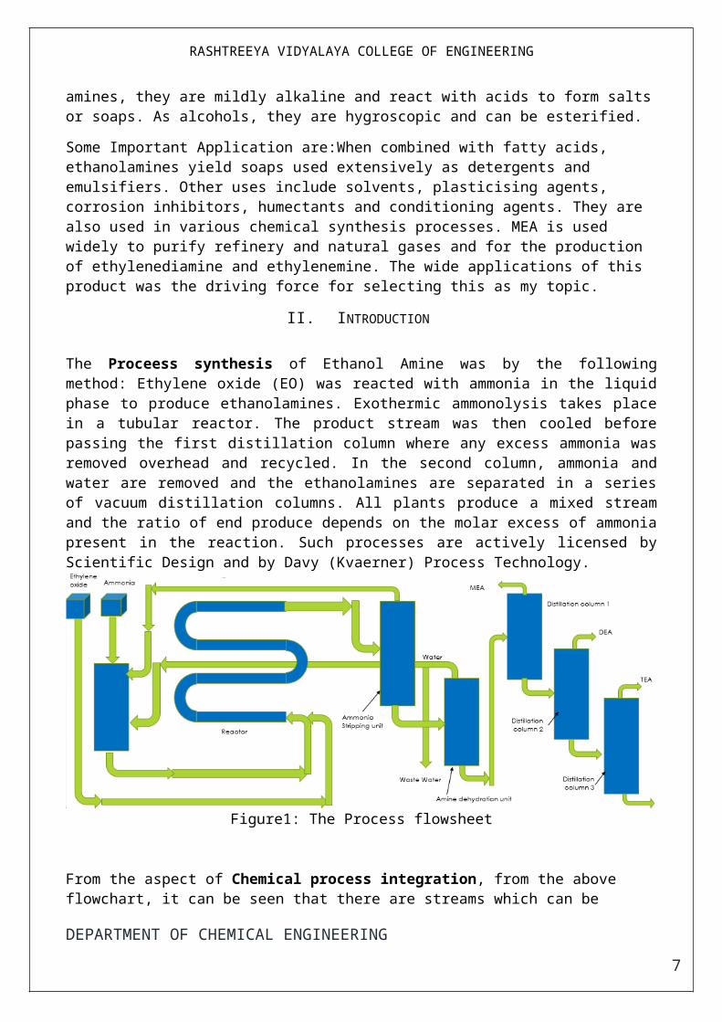
The Proceess synthesis of Ethanol Amine was by the following method: Ethylene oxide (EO) was reacted with ammonia in the liquid phase to produce ethanolamines. Exothermic ammonolysis takes place in a tubular reactor. The product stream was then cooled before passing the first distillation column where any excess ammonia was removed overhead and recycled. In the second column, ammonia and water are removed and the ethanolamines are separated in a series of vacuum distillation columns. All plants produce a mixed stream and the ratio of end produce depends on the molar excess of ammonia present in the reaction. Such processes are actively licensed by Scientific Design and by Davy (Kvaerner) Process Technology.


6


Figure1: The Process flowsheet

From the aspect of Chemical process integration, from the above flowchart, it can be seen that there are streams which can be recycled. From ammonia stripping unit, unreacted ammonia can be recycled. The waste water from the amine dehydration unit can be recycled back to the reactor. By recycling the waste streams, the terminal discharge of the plant is reduced. The cost of production is reduced.

From the engineering economics point of view, a study must be carried out which includes the major steps to be incorporated before setting up a manufacturing unit, they are:

1. Stages for Plant design project:2. Feasibility survey3. Process Development4. Equipment design and selection5. Plant location6. Cost Analysis and estimation

Design Consideration of Ethanol Amine Manufacturing: (Economics)

There were several specific problems involved in the design of this reactor system. First, the solvent characteristics of the reaction needed to be determined. An anhydrous reaction would be simple and clean, but the reaction would have to occur in the liquid phase, and requiring compression of the ammonia to liquid phase would be a costly operation. The second option is to allow the reaction to occur in aqueous phase, thus allowing the ammonia to stay liquefied under lower pressures. This would also be a good method of reducing the reactivity of ethylene, for safety purposes (ethylene oxide can be explosive). The disadvantage is that the water would have to be separated later from the product stream, and also the fact that if anytime during the process the temperature or pressure of the process stream is too high, the ethylene oxide will react with the water to form ethylene glycol. It was decided to carry out the reaction in the aqueous phase because the safety gained with aqueous ethylene oxide and money saved by putting ammonia into solution would outweigh the cost of a separator and the glycol reaction would be minimal (rate of glycol formation doesn’t begin to become near significant until about 430 C, and as will be discussed later the reaction never will reach temperature above 200 C).


7


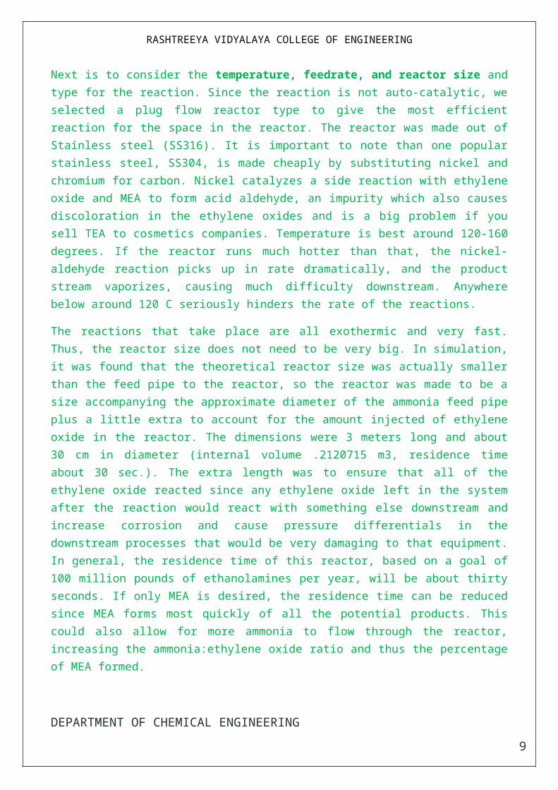
Next is to consider the temperature, feedrate, and reactor size and type for the reaction. Since the reaction is not auto-catalytic, we selected a plug flow reactor type to give the most efficient reaction for the space in the reactor. The reactor was made out of Stainless steel (SS316). It is important to note than one popular stainless steel, SS304, is made cheaply by substituting nickel and chromium for carbon. Nickel catalyzes a side reaction with ethylene oxide and MEA to form acid aldehyde, an impurity which also causes discoloration in the ethylene oxides and is a big problem if you sell TEA to cosmetics companies. Temperature is best around 120-160 degrees. If the reactor runs much hotter than that, the nickel-aldehyde reaction picks up in rate dramatically, and the product stream vaporizes, causing much difficulty downstream. Anywhere below around 120 C seriously hinders the rate of the reactions.

The reactions that take place are all exothermic and very fast. Thus, the reactor size does not need to be very big. In simulation, it was found that the theoretical reactor size was actually smaller than the feed pipe to the reactor, so the reactor was made to be a size accompanying the approximate diameter of the ammonia feed pipe plus a little extra to account for the amount injected of ethylene oxide in the reactor. The dimensions were 3 meters long and about 30 cm in diameter (internal volume .2120715 m3, residence time about 30 sec.). The extra length was to ensure that all of the ethylene oxide reacted since any ethylene oxide left in the system after the reaction would react with something else downstream and increase corrosion and cause pressure differentials in the downstream processes that would be very damaging to that equipment. In general, the residence time of this reactor, based on a goal of 100 million pounds of ethanolamines per year, will be about thirty seconds. If only MEA is desired, the residence time can be reduced since MEA forms most quickly of all the potential products. This could also allow for more ammonia to flow through the reactor, increasing the ammonia:ethylene oxide ratio and thus the percentage of MEA formed.

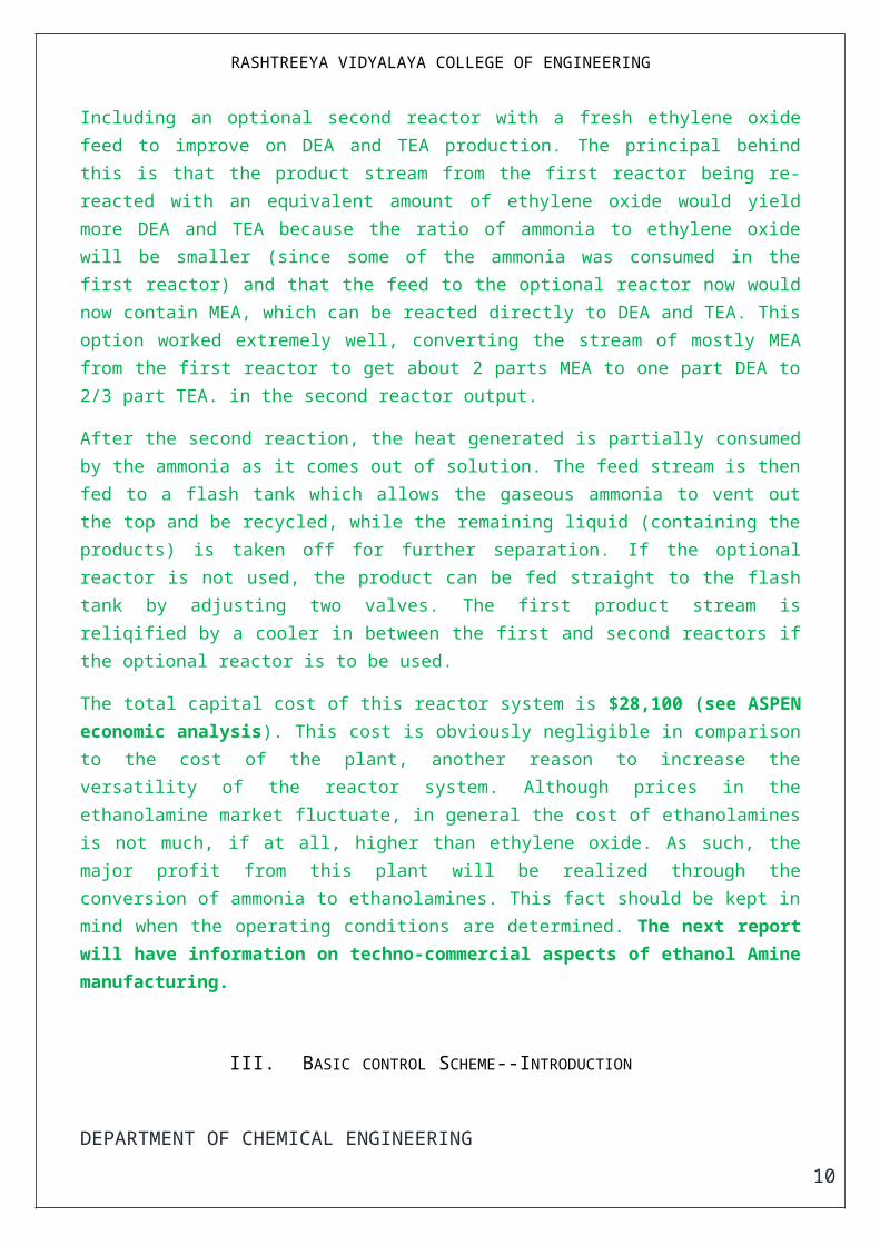
Including an optional second reactor with a fresh ethylene oxide feed to improve on DEA and TEA production. The principal behind this is that the product stream from the first reactor being re-reacted with an equivalent amount of ethylene oxide would yield more DEA and TEA because the ratio of ammonia to ethylene oxide will be smaller (since some of the ammonia was consumed in the first reactor) and that the feed to the optional reactor now would now contain MEA, which can be reacted directly to DEA and TEA. This option worked extremely well, converting the stream of mostly MEA from the first reactor to get about 2 parts MEA to one part DEA to 2/3 part TEA. in the second reactor output.

After the second reaction, the heat generated is partially consumed by the ammonia as it comes out of solution. The feed stream is then fed to a flash tank which allows the gaseous ammonia to vent out the top and be recycled, while the remaining liquid (containing the products) is taken off for further separation. If the optional reactor is not used, the product can be fed straight to the flash tank by adjusting two valves. The first product stream is reliqified by a cooler in between the first and second reactors if the optional reactor is to be used.

The total capital cost of this reactor system is $28,100 (see ASPEN economic analysis). This cost is obviously negligible in comparison to the cost of the plant, another reason to increase the versatility of the reactor system. Although prices in the ethanolamine market fluctuate, in general the cost of ethanolamines is not much, if at all, higher than ethylene oxide. As such, the major profit from this


8


plant will be realized through the conversion of ammonia to ethanolamines. This fact should be kept in mind when the operating conditions are determined. The next report will have information on techno-commercial aspects of ethanol Amine manufacturing.

III. BASIC CONTROL SCHEME--INTRODUCTION

Procedure:

It is not a trivial task to develop a systematic procedure for the design of control schemes for process units and entire plants. It is even not without risk, since the designer may think that by following the procedure the task will be completely finished. But it is of extreme importance to verify an intermediate result in different ways and if necessary to start the design procedure all over again.

It is not very meaningful to search for the ultimate control scheme for a particular process. The magnitude and nature of disturbances, the frequency of changes and the way the process is operated (for example at maximum load or maximum efficiency), the flexibility of the plant and the knowledge of operating and maintenance personnel all play a crucial role in the control scheme selection process. It is very well possible, that a particular process is heavily instrumented and automated in one plant and is hardly automated in another plant. It is therefore recommended to review the control scheme after the plant has come online and make changes in the control scheme if required.

Sometimes, the expansion of a plant can have consequences for control of the older part of the plant. For example, after an expansion of the number of boilers, it is advantageous to operate a new boiler at full load, since it has a higher efficiency than the older boilers. This also has consequences for the control scheme for the older boilers, which should cope with the changes in steam demand.

The next sequence of steps can be used as a design procedure, or as a checklist afterwards if one prefers a more intuitive approach to control system design. The checklist is more or less similar to the checklist for the development of an environmental model .

i. Operation of the processii. Goals of the operationiii. Process boundaries and external disturbancesiv. Controlled process conditions, accumulation variables and qualitiesv. Throughput/load and recycle flowsvi. Correcting variablesvii. Interaction table and count of degrees of freedomviii. Power and speed of controlix. Basic control scheme

(i) Operation of the process: Study the operation of the process. It is essential to understand why the process equipment is there, what its function is. The same holds for every


9


process flow. Close contact with process developers and process designers is very useful at this point.

(ii) Goals of the operation: The goals of the operation are dictated by a hierarchically higher operational layer. For a plant, the goal is usually to produce a certain or maximum quantity (throughput) with a pre-defined quality. In addition, requirements may exist for side streams, waste streams and energy supply (temperature level). The goal is in that case to produce a desired quality and quality at minimum costs, in other words, minimum use of feed and energy. Different control goals result consequently in different control schemes.

a. a varying liquid flow (from a previous process) or maximum liquid flow is heated to a required temperature. b. a desired liquid flow is heated to a required temperature. c. all steam supply is used to heat the liquid flow to a required temperature. d. a maximum flow of steam is condensed by a maximum liquid flow.

(iii) Process boundaries and external disturbances: Investigate whether the boundaries of the process are also correct for the design of the control scheme. Pay special attention to utilities (steam, electricity, flue gas) and exchange of energy and material, which can lead to a widening of the process boundaries. It would be an advantage if the process could be sub-divided into independent sub-processes for which a control scheme could then be developed separately.

(iv) Controlled variables: The controlled variables can be classified into three categories: process conditions, material contents and qualities. • Controlled process conditions. The conditions of different process units have to be maintained at their design specification. This concerns in particular pressures (of reactors, columns, furnaces, etc), temperatures (of reactors), and residence times (of reactors).

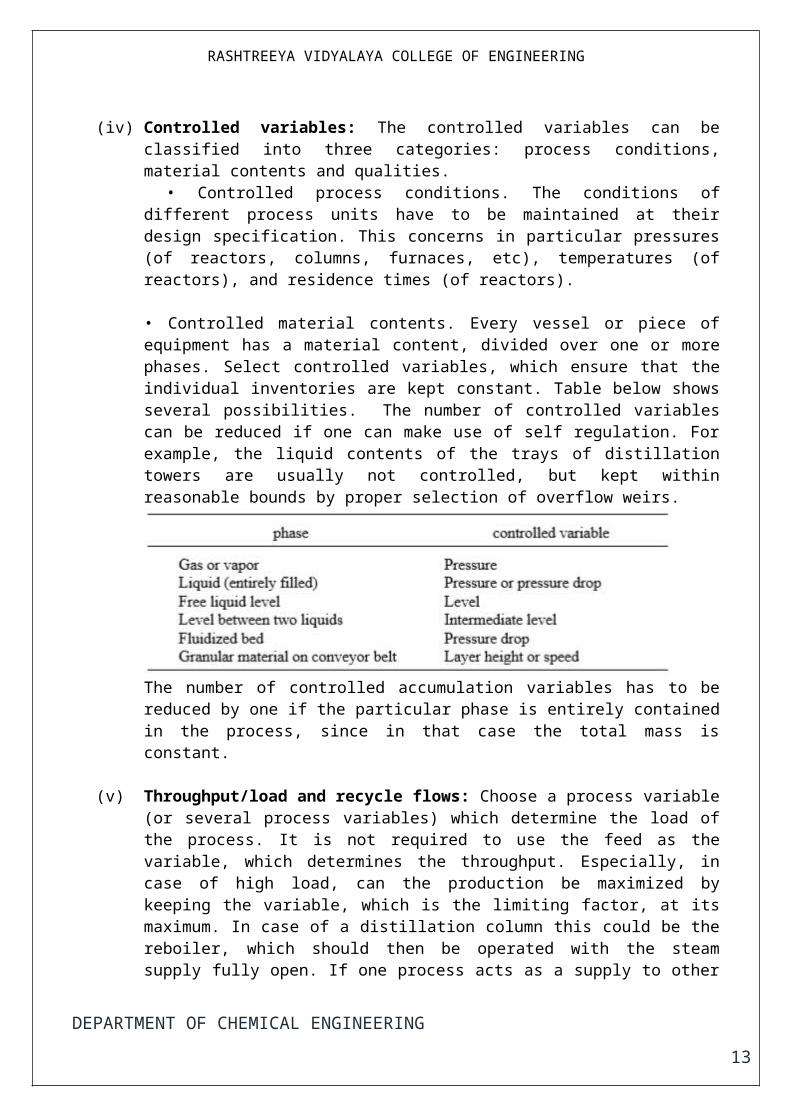
• Controlled material contents. Every vessel or piece of equipment has a material content, divided over one or more phases. Select controlled variables, which ensure that the individual inventories are kept constant. Table below shows several possibilities. The number of controlled variables can be reduced if one can make use of self regulation. For example, the liquid contents of the trays of distillation towers are usually not controlled, but kept within reasonable bounds by proper selection of overflow weirs.

The number of controlled accumulation variables has to be reduced by one if the particular phase is entirely contained in the process, since in that case the total mass is constant.

(v) Throughput/load and recycle flows: Choose a process variable (or several process variables) which determine the load of the process. It is not required to use the feed as the


10


variable, which determines the throughput. Especially, in case of high load, can the production be maximized by keeping the variable, which is the limiting factor, at its maximum. In case of a distillation column this could be the reboiler, which should then be operated with the steam supply fully open. If one process acts as a supply to other processes, for example a central steam boiler, then the throughput is usually determined by the consumer(s). Recycle flows can best be kept at constant flow or flow ratio, this reduces the propagation of disturbances. Disturbance propagation is more difficult to control if the recycle flow includes multiple process units.

(vi) Correcting variables: For total control, all process flows should be adjustable, hence in principle every process flow is a candidate for a correcting variable. This only holds under the condition that the accumulations are automatically controlled: every form of self-regulation decreases the number of correcting variables. Investigate whether it is economically feasible to adjust the correcting variables by control valves. Control valves for pipelines with large diameter are very expensive and consume large amounts of mechanical energy. They can be omitted unless the controllability of the process is negatively affected. An alternate for control valves are speed controllers of pumps, compressors and turbines. This is especially interesting because of the high cost of energy. Already interesting options exist for asynchronous motors. A simple rule of thumb for the selection of adjustable process variables is:

Every incoming flow that has not been determined externally, should be controlled, except when the flow is established as a result of self-regulation of the adjustable mass- or energy accumulation. The positioning of a valve, which creates an extra accumulation that has to be controlled, is not allowed. Similarly, two valves in a pipeline (without creating a meaningful accumulation) is not allowed either. If a flow is separated into two other flows, only two of the three flows may contain a control valve.

Examples of flows that do not have to be controlled or should not be controlled are: • no valve should be positioned in the discharge line of a thermo-syphon reboiler, since free circulation is required. • no valve should be positioned in a multiphase flow of vapor and liquid between a condenser and accumulator, since the liquid flow into the accumulator as a result of gravity should be unobstructed. • no valve should be positioned in a supply or discharge line of an evaporator or condensor, since the amount of liquid that evaporates or vapor that condenses, is directly determined by the energy supply or removal. • no valve should be positioned between pressure vessels if the pressure drop is relatively small, since otherwise an undesired pressure drop is created, one of the pressures will follow the other one which is controlled and is therefore more or less self-regulating. • valves should not be present in fluidized flows, the gas and solids flows have to be adjusted separately.

(vii) Interaction table and count of degrees of freedom: The procedure for the development of the control scheme deviates from the procedure for the development of an environmental model. The controlled variables now have to be arranged in a table versus the correcting variables. The table is used to represent power and speed of control for each combination of variables.


11


Compare the number of correcting variables with the number of controlled variables. If there are fewer correcting variables than controlled variables, the previous steps have to be reviewed. There is obviously no guarantee that no errors have been made. Sometimes the review process is equivalent to determining a relationship between controlled variables.

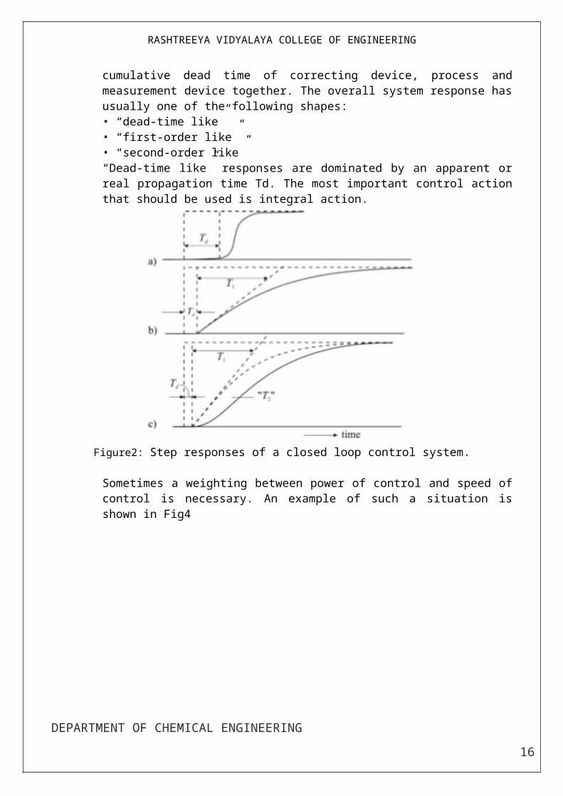
(viii) Power of control and speed of control: For each combination of the controlled and correcting variables in the Table, the power and speed of control have to be established. The quality of control that can be expected for an automatic control loop, is characterized by the power of control and speed of control. The power of control is a measure for the static impact of the correcting variable on the controlled variable. If this impact is small or negligible, then the corresponding control loop will not function properly. The speed of control is a measure for the dynamic impact. This can be expressed by the oscillation frequency for proportional control close to the limit of stability. The higher the frequency, the better disturbances can be eliminated. The speed of control is limited by the apparent dead time in the control loop, which is the cumulative dead time of correcting device, process and measurement device together. The overall system response has usually one of the following shapes:• “dead-time like” • “first-order like” • “second-order like” “Dead-time like” responses are dominated by an apparent or real propagation time Td. The most important control action that should be used is integral action.

Figure2: Step responses of a closed loop control system.

Sometimes a weighting between power of control and speed of control is necessary. An example of such a situation is shown in Fig4


12


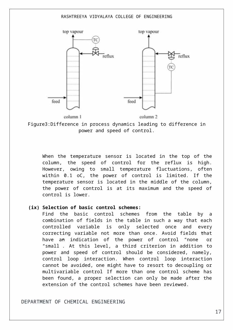
Figure3:Difference in process dynamics leading to difference in power and speed of control.

When the temperature sensor is located in the top of the column, the speed of control for the reflux is high. However, owing to small temperature fluctuations, often within 0.1 oC, the power of control is limited. If the temperature sensor is located in the middle of the column, the power of control is at its maximum and the speed of control is lower.

(ix) Selection of basic control schemes:Find the basic control schemes from the table by a combination of fields in the table in such a way that each controlled variable is only selected once and every correcting variable not more than once. Avoid fields that have an indication of the power of control “none” or “small”. At this level, a third criterion in addition to power and speed of control should be considered, namely, control loop interaction. When control loop interaction cannot be avoided, one might have to resort to decoupling or multivariable control If more than one control scheme has been found, a proper selection can only be made after the extension of the control schemes have been reviewed.

IV. OPTIMAL CONTROL

So far, we have only discussed control loops that keep process conditions constant or reject disturbances, thereby avoiding undesirable process conditions. One could go one step further and try to keep the process in an optimal operating point. A checklist for items to be addressed is shown in Table below:

Optimal control

i. Degrees of freedom for optimizationii. Constraintsiii. Model iv. Optimal operating point


13


v. Active constraints vi. Degrees of freedom for consideration

Since the optimal operating point depends on the “mode of operation”, high demands are imposed on the optimal control structure. The control scheme must be able to switch to different constraints if they become active.

(i, ii) Degrees of freedom for optimization and constraints: One should investigate which setpoints of the basic control scheme are candidates for an optimal setting. The same holds for the remaining correcting variables if any. For the desulphurization process (Fig. 33.5), this investigation yields the following list of variables:• inlet temperature of the reactor • intermediate temperatures of the reactor • pressure reactor • hydrogen-crude oil ratio • hydrogen or hydrogen sulfide fractionThe separator level does not appear in this list, since the level does not have any impact on the operation of the process (there is no optimal value of the level). The oxygen controller takes care of a local optimization by maintaining a small excess air to fuel ratio. For every process unit and process flow the limits should be determined between normal and abnormal operation.

(iii) Model: For continuous process operation a static model will suffice, supplemented with the constraints inequalities. It is not easy to develop a good model, since process knowledge is usually limited and inaccurate.

(iv) Optimal operating point: By using an optimization algorithm for the static model with its constraints, the optimal operating point is determined as a function of the independent variables. In most cases the optimum is located on a constraint or the intersection of several constraints. Hardly ever is the optimum a free optimum.

(v) Active constraints: The optimal operating point could be located on different constraints, hence, those constraints are active. For different operating conditions identify groups of constraints that are active. Investigate whether these groups of constraints can be controlled by their own correcting variable. If so, a selecting control system can be developed.

Example: Capacities distillation column In a distillation column, the condenser capacity, the tray capacity (maximum tray pressure drop) or the reboiler capacity are limiting factors for the operation. This will be explained in more detail in the next report.

(vi) Degrees of freedom for consideration: If the optimal operating point is not located on active constraints, the optimum is determined by “degrees of freedom for consideration”. Try to find an approximate model, representing the values of these degrees of freedom as a function of the independent variables or certain dependent variables.

Example: Reboiler heat distillation column Sometimes the heat flow in the reboiler of a distillation column is a degree of freedom for consideration. This heat flow has to be approximately proportional to the feed flow. This points at using a ratio control between the feed and the heat flow to the reboiler. This ratio can be a function of the pressure in the column (affecting the separation) and specific costs.

Extension of the Control Scheme:DEPARTMENT OF CHEMICAL ENGINEERING

14


In this section several examples will be given of extensions of the control scheme. Issues that will be discussed are:i. Cascade control. One control loop sets the setpoint of another control loop. Goals for control

that are hierarchical, are reflected in the control structure.ii. Feed-forward control. This provides compensation for measurable disturbances. In this case

disturbance information is used in the control scheme. iii. Compensators. Often process behavior exhibits a dead time or inverse response in which

case model-based control may be advantageous.iv. Selectors. This implies switching between controllers and/or sensors. v. Split-range control. This involves selection of controllers based on the range.

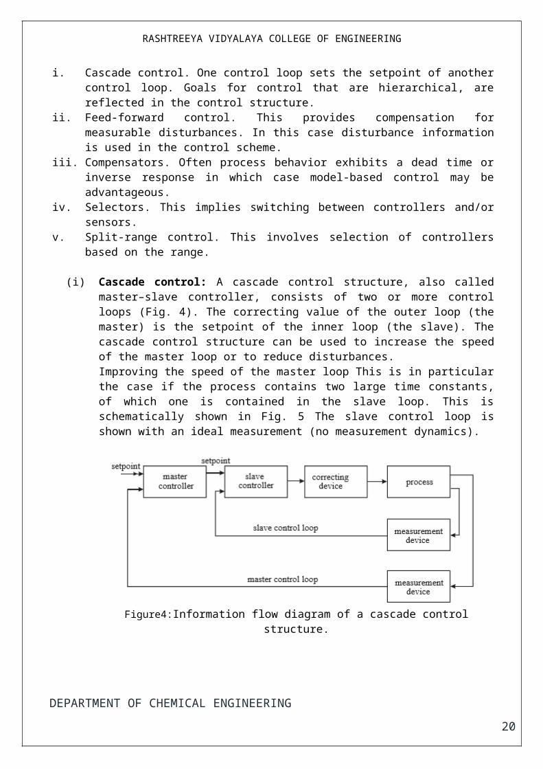
(i) Cascade control: A cascade control structure, also called master–slave controller, consists of two or more control loops (Fig. 4). The correcting value of the outer loop (the master) is the setpoint of the inner loop (the slave). The cascade control structure can be used to increase the speed of the master loop or to reduce disturbances.Improving the speed of the master loop This is in particular the case if the process contains two large time constants, of which one is contained in the slave loop. This is schematically shown in Fig. 5 The slave control loop is shown with an ideal measurement (no measurement dynamics).

Figure4:Information flow diagram of a cascade control structure.

Figure5: Slave control loop.

The transfer function from x to y can be written as:


15


When τ1 = 10 minutes and K = 9, the slave control loop can be replaced by a firstorder transfer function with a time constant of 1 minute. The value of the gain K is usually limited by secondary effects, such as non-linearities and smaller time constants, which also play a role).Example: Reboiler level distillation column:

Suppose in an evaporator as shown in Fig.6, the evaporation is controlled by a level controller, thus affecting the heat transfer area. However, the dynamic response is quite slow and can be represented by a first-order response with a large time constant. In order to reduce the effect of the large time constant in the condensate level, a cascade controller should be used. The steam supply is controlled by a flow controller, which determines the setpoint of the level controller. The flow controller will keep the steam supply constant regardless of disturbances in the steam supply pressure.

Figure6: Cascade control for an evaporator.

Reduction of disturbances that can be measured inside the slave controller This is only relevant if the slave controller is faster than the master controller. An example of the use in reactor temperature control is shown in Fig. 7.


16


Figure7: Cascade controller structure for reactor.

(ii) Feed-forward control: If a measurable disturbance shows large variations and the process is slow, feedback control may not suffice. In that case it is possible to use anticipating action or feed-forward control. Figure 8 shows the general information flow diagram.

Figure8:Information flow diagram for feed-forward control.

A disturbance is measured and passed on to the controlled variable via the correcting variable. Variations in the controlled variable as a result of the disturbance are exactly compensated for if the transfer functions along the two paths are identical:

G1+G2G3=0The transfer function of the controller should therefore, under all operating conditions, be represented by the equation:

G 3=G 2/G 1which requires sometimes extensive process testing and which is, in some cases, impossible to realize. Example: if G1 contains no dead time and G2 does, G3 should contain a negative dead time.

(iii) Compensators: Many processes can exhibit dynamics that are detrimental to good control. Examples are the presence of a process dead time or inverse dynamics. Assume that we are able to factor the process dynamics into two parts, one that we shall call reversible process dynamics and another part that will be called irreversible dynamics. An


17


example is shown in Fig.9, part a shows how the controller will be configured and part b shows the equivalent block diagram in case of an ideal process model. The denominator of the transfer function from ysp to y becomes now GCGP,rev instead of GCGP, as a result of which the dynamics of the closed loop response have become considerably faster.

Figure9: Process control with compensation for irreversible dynamics.

(iv) Use of selectors: A “high” or “low-value” selector can be very useful in case of constraint control. An example is a furnace in which different temperatures are measured, none of them may become too excessive. A controller can be connected to the fuel supply, via “high-value” selectors (see Fig. 10), such that the controller only acts on the highest measured value.

Figure10: Selector control for a furnace.

Figure 11 shows a selecting measurement system. The tray loading in a distillation column is monitored at three locations, the highest value is passed on to a pressure difference controller manipulating the cooling water flow to the condensor.


18


Figure11: Selecting measurement system for a distillation column

(v) Override control: Complicated control loops, in which cascade control, ratio control and selectors are applied, can be found in furnace control. Usually, the outlet temperature is controlled automatically. This is most likely also the highest temperature that the feed will experience. For safety reasons, the control structure is realized by adjusting the fuel supply, often via a slave controller. The advantages of this slave controller are: • Disturbances in the fuel supply pressure are eliminated by the fast slave controller

• In case of liquid fuel, the burner pressure can be maintained above a minimum value, which is required for good atomization of the liquid. This can be achieved by a “high value” selector H: an instrument that passes on the highest measurement only.

(vi) Split-range control: Figure 12 shows temperature control in the jacket of a chemical reactor by introduction of cooling water or steam. The controller manipulates two valves with separated range (“split range”): after the cooling water valve is fully closed, the steam valve is opened and vice versa. For smooth control it is desired that there is a small overlap, as shown in Fig. 13. The division of the total range should be selected in such a way that the proportional action of the controller can be set at the same value for water and steam.


19


Figure12: Jacket temperature control.

Figure13: Overlapping ranges

V. CONCLUSION AND ACKNOWLEDGEMENT

There are many process synthesis techniques for preparation of ethanolamine. A process flowsheet was selected and explained. The streams available for recycle were found out from the flowsheet. Economics aspects were incorporated into the manufacturing of ethanoamine and finally the process dynamics aspects, the basic control scheme, the brief outline was highlighted. I thank our professors in giving an opportunity to learn about such processes which will prove to be helpful in the furture. Continuation of this report will be given after the second Phase.

REFERENCES

[1.] Cohen, G.H. and Coon, G.A. (1953) Theoretical considerations of retarded control. Transactions of the American Society of Mechanical Engineers, 75, 827–34.

[2.] Ziegler, J.G. and Nichols, N.B. (1942) Optimum settings for automatic controllers. Transactions of the American Society of Mechanical Engineers, 62, 759–68.


20


[3.] Betlem, B.H.L. (1998) Influence of tray hydraulics on tray column dynamics. Chemical Engineering Science, 53, 3991–4003.

[4.] Grinten P.M.E.M. van der (1970), Procesregelingen, Prisma-Technica 140, Spectrum, Utrecht.

[5.] Luyben W.L. (ed.) (1992) Practical Distillation Control, Van Nostrand Reinhold, New York. Shinskey F.G. (1984) Distillation Control, McGraw-Hill, New York.

[6.] Rademaker O., Rijnsdorp, J.E. and Maarlevelt, A. (1975) Dynamics and Control of Continuous Distillation Units, Elsevier Scientific Publishing Company, Amsterdam.

[7.] Ryskamp C.J. (1980) New strategy improves dual composition column control. Hydrocarbon Processing, June, 51–9.

[8.] S. J. Benz1 and N. J. Scennal, “An Extensive Analysis on the Start-Up of a Simple Distillation Column with Multiple Steady States,” The Canadian Journal of Chemical Engineering, Vol. 80, No. 5, 2002, pp. 865-881. doi:10.1002/cjce.5450800510

[9.] N. Sharma and K. Singh, “Control of Reactive Distillation Column: A Review,” International Journal of Chem- ical Reactor Engineering, Vol. 8, No. 1, 2010

[10.] S. Skogestad and M. Morari, “The Dominate Time Constant for Distillation Columns,” Computers & Chemical Engineering, Vol. 11, No. 6, 1987, pp. 607-617. doi:10.1016/0098-1354(87)87006-0

[11.] “Process Dynamics and Control Modeling for Control and Prediction” by Brian Roffel and Ben Betlem, ISBN-13: 978-0-470-01663-3 (HB)


self study reort 1-ashwanth+economics

Documents

process control

selector control

speed of control

optimal control

cascade control structure

feedforward control

slave control loop136

jacket temperature control