sensor-driven hierarchical path planning for unmanned
TRANSCRIPT
Brigham Young University Brigham Young University
BYU ScholarsArchive BYU ScholarsArchive
Theses and Dissertations
2013-09-23
Sensor-Driven Hierarchical Path Planning for Unmanned Aerial Sensor-Driven Hierarchical Path Planning for Unmanned Aerial
Vehicles Using Canonical Tasks and Sensors Vehicles Using Canonical Tasks and Sensors
Spencer James Clark Brigham Young University - Provo
Follow this and additional works at: https://scholarsarchive.byu.edu/etd
Part of the Computer Sciences Commons
BYU ScholarsArchive Citation BYU ScholarsArchive Citation Clark, Spencer James, "Sensor-Driven Hierarchical Path Planning for Unmanned Aerial Vehicles Using Canonical Tasks and Sensors" (2013). Theses and Dissertations. 3798. https://scholarsarchive.byu.edu/etd/3798
This Thesis is brought to you for free and open access by BYU ScholarsArchive. It has been accepted for inclusion in Theses and Dissertations by an authorized administrator of BYU ScholarsArchive. For more information, please contact [email protected], [email protected].

Sensor-Driven Hierarchical Path Planning for Unmanned Aerial
Vehicles Using Canonical Tasks and Sensors
Spencer J. Clark
A thesis submitted to the faculty ofBrigham Young University
in partial fulfillment of the requirements for the degree of
Master of Science
Michael A. Goodrich, ChairBryan S. Morse
Dennis Ng
Department of Computer Science
Brigham Young University
October 2013
Copyright © 2013 Spencer J. Clark
All Rights Reserved

ABSTRACT
Sensor-Driven Hierarchical Path Planning for Unmanned AerialVehicles Using Canonical Tasks and Sensors
Spencer J. ClarkDepartment of Computer Science, BYU
Master of Science
Unmanned Aerial Vehicles (UAVs) are increasingly becoming economical platformsfor carrying a variety of sensors. Building flight plans that place sensors properly, temporallyand spatially, is difficult. The goal of sensor-driven planning is to automatically generateflight plans based on desired sensor placement and temporal constraints. We propose asimple taxonomy of UAV-enabled sensors, identify a set of generic sensor tasks, and arguethat many real-world tasks can be represented by the taxonomy. We present a hierarchicalsensor-driven flight planning system capable of generating 2D flights that satisfy desiredsensor placement and complex timing and dependency constraints. The system makes use ofseveral well-known planning algorithms and includes a user interface. We conducted a userstudy to show that sensor-driven planning can be used by non-experts, that it is easier fornon-experts than traditional waypoint-based planning, and that it produces better flightsthan waypoint-based planning. The results of our user study experiment support the claimsthat sensor-driven planning is usable and that it produces better flights.
Keywords: Flight planning, unmanned aerial vehicles, UAVs

Table of Contents
List of Figures vi
List of Tables viii
1 Introduction 1
1.1 Delimitations . . . . . . . . . . . . . . . . . . . . . . . . . . . . . . . . . . . 4
2 Related Work 5
2.1 UAV Flight Planning . . . . . . . . . . . . . . . . . . . . . . . . . . . . . . . 5
2.2 Sensor Taxonomies . . . . . . . . . . . . . . . . . . . . . . . . . . . . . . . . 9
3 Taxonomy 10
3.1 Sensors . . . . . . . . . . . . . . . . . . . . . . . . . . . . . . . . . . . . . . . 10
3.2 Tasks . . . . . . . . . . . . . . . . . . . . . . . . . . . . . . . . . . . . . . . . 11
3.3 Constraints . . . . . . . . . . . . . . . . . . . . . . . . . . . . . . . . . . . . 11
3.4 Areas . . . . . . . . . . . . . . . . . . . . . . . . . . . . . . . . . . . . . . . . 12
3.5 Summary . . . . . . . . . . . . . . . . . . . . . . . . . . . . . . . . . . . . . 12
4 User Interface 14
4.1 Dubins Curves . . . . . . . . . . . . . . . . . . . . . . . . . . . . . . . . . . . 14
4.2 Defining Planning Problems . . . . . . . . . . . . . . . . . . . . . . . . . . . 15
4.3 Planning . . . . . . . . . . . . . . . . . . . . . . . . . . . . . . . . . . . . . . 19
4.4 Alternative Planning Interfaces . . . . . . . . . . . . . . . . . . . . . . . . . 20
iii

5 Hierarchical Planning 24
5.1 Task Start Position and Pose . . . . . . . . . . . . . . . . . . . . . . . . . . 26
5.2 Sub-Flight Planning . . . . . . . . . . . . . . . . . . . . . . . . . . . . . . . 27
5.3 Scheduler . . . . . . . . . . . . . . . . . . . . . . . . . . . . . . . . . . . . . 28
5.4 Intermediate Planner . . . . . . . . . . . . . . . . . . . . . . . . . . . . . . . 31
5.5 Performance Considerations . . . . . . . . . . . . . . . . . . . . . . . . . . . 32
6 Sub-Flight Planning 37
6.1 Discretized Position/Orientation Statespace . . . . . . . . . . . . . . . . . . 37
6.2 Best-First Tree Search . . . . . . . . . . . . . . . . . . . . . . . . . . . . . . 39
6.3 Best-First Search in Discretized Position/Orientation Statespace . . . . . . . 39
6.4 Genetic Algorithm in Discretized Position/Orientation Statespace . . . . . . 42
6.5 Simple Greedy Search in Discretized Position/Orientation Statespace . . . . 42
6.6 Comparison . . . . . . . . . . . . . . . . . . . . . . . . . . . . . . . . . . . . 42
7 User Study 48
7.1 Secondary Task . . . . . . . . . . . . . . . . . . . . . . . . . . . . . . . . . . 49
7.2 Waypoint Planner . . . . . . . . . . . . . . . . . . . . . . . . . . . . . . . . . 52
7.3 Flight Testing . . . . . . . . . . . . . . . . . . . . . . . . . . . . . . . . . . . 53
7.4 Measurements and Procedures . . . . . . . . . . . . . . . . . . . . . . . . . . 55
7.5 Pilot Study . . . . . . . . . . . . . . . . . . . . . . . . . . . . . . . . . . . . 58
7.6 Results . . . . . . . . . . . . . . . . . . . . . . . . . . . . . . . . . . . . . . . 58
7.6.1 Usability . . . . . . . . . . . . . . . . . . . . . . . . . . . . . . . . . . 59
7.6.2 Ease of Use . . . . . . . . . . . . . . . . . . . . . . . . . . . . . . . . 61
7.6.3 Quality of Flights . . . . . . . . . . . . . . . . . . . . . . . . . . . . . 61
7.7 Summary . . . . . . . . . . . . . . . . . . . . . . . . . . . . . . . . . . . . . 63
8 Conclusions 66
8.1 Conclusions . . . . . . . . . . . . . . . . . . . . . . . . . . . . . . . . . . . . 66
iv

8.2 Future Work . . . . . . . . . . . . . . . . . . . . . . . . . . . . . . . . . . . . 68
Appendices 70
A User Study Briefings, Surveys, etc. . . . . . . . . . . . . . . . . . . . . . . . 71
References 79
v
List of Figures
1.1 The status quo compared with the goals of sensor-driven flight planning. . . 3
4.1 Comparison of using Dubins curves vs. straight lines for connecting waypoints. 16
4.2 Screenshot of the main sensor driven graphical user interface (GUI). . . . . . 17
4.3 Editing task areas in the GUI as polygons. . . . . . . . . . . . . . . . . . . . 17
4.4 Screenshot of the GUI’s task area editor dialog. . . . . . . . . . . . . . . . . 18
4.5 Screenshot of the GUI’s task editor dialog. . . . . . . . . . . . . . . . . . . . 19
4.6 The results of a planning operation displayed in the GUI. . . . . . . . . . . . 20
4.7 A screenshot of Procerus’s “Virtual Cockpit” UAV flight planner. . . . . . . 21
4.8 A screenshot of the BYU HCMI lab’s Phairwell user interface. . . . . . . . . 22
4.9 Another UAV flight system developed by the BYU HCMI lab. . . . . . . . . 22
4.10 Relationships between the components of the 2nd-generation WiSAR interface. 23
5.1 The pieces of a flight generated by the hierarchical planner. . . . . . . . . . . 25
5.2 Heuristic for selecting starting positions and poses for flight tasks. . . . . . . 27
5.3 The scheduler’s A* state space with a small example. . . . . . . . . . . . . . 30
5.4 Scheduler performance benchmarks. . . . . . . . . . . . . . . . . . . . . . . . 34
5.5 A contrived highly-constrained scenario. . . . . . . . . . . . . . . . . . . . . 35
6.1 Calculation of discretized position/orientation space. . . . . . . . . . . . . . 38
6.2 Illustration of the parameters of the best-first tree search. . . . . . . . . . . . 40
6.3 Flight length and required planning time for “difficult” evaluation scenarios. 47
7.1 An example briefing document from the user study. . . . . . . . . . . . . . . 50
vi

7.2 The secondary task (simulated chat) for the user study. . . . . . . . . . . . . 52
7.3 Screenshot of the waypoint-based comparison interface. . . . . . . . . . . . . 54
7.4 User study procedure for experiment sequence A1—B1—C2—D2. . . . . . . 56
7.5 Illustration of improved polygon drawing functionality. . . . . . . . . . . . . 65
A.1 Briefing document for user study scenario A. . . . . . . . . . . . . . . . . . . 72
A.2 Briefing document for user study scenario B. . . . . . . . . . . . . . . . . . . 73
A.3 Briefing document for user study scenario C. . . . . . . . . . . . . . . . . . . 74
A.4 Briefing document for user study scenario D. . . . . . . . . . . . . . . . . . . 75
A.5 Briefing document for user study practice scenario E. . . . . . . . . . . . . . 76
A.6 Briefing document for user study practice scenario F. . . . . . . . . . . . . . 76
A.7 Screenshot of the web-based NASA-TLX survey used after each user study
scenario. . . . . . . . . . . . . . . . . . . . . . . . . . . . . . . . . . . . . . . 77
A.8 The questions used in the demographics survey. . . . . . . . . . . . . . . . . 77
A.9 The questions used in the post-user study survey. . . . . . . . . . . . . . . . 78
vii

List of Tables
1.1 Examples of UAV users, uses, and sensors. . . . . . . . . . . . . . . . . . . . 1
3.1 Examples of the combinations of canonical tasks and sensors. . . . . . . . . . 11
5.1 Reward functions for the sub-flight planner. . . . . . . . . . . . . . . . . . . 28
6.1 Parameters for sub-flight algorithm comparison and benchmarking. . . . . . 45
6.2 Results of sub-flight comparison on the “easy” scenarios. . . . . . . . . . . . 46
6.3 Results of sub-flight comparison on the “difficult” scenarios. . . . . . . . . . 47
7.1 Summary of the four scenarios used in the user study. . . . . . . . . . . . . . 49
7.2 User study counterbalancing permutations. . . . . . . . . . . . . . . . . . . . 51
7.3 The means of the measurements for sensor-driven planning and waypoint-based
planning methods. Significant results in bold. . . . . . . . . . . . . . . . . . 59
7.4 A summary of the practical and statistical significance of the user study results.
Significant results in bold. . . . . . . . . . . . . . . . . . . . . . . . . . . . . 60
7.5 Comparison of the length of flights generated using the two planning methods. 63
viii

Chapter 1
Introduction
Unmanned aerial vehicles (UAVs) are frequently used as sensor platforms. They are
capable of carrying a wide variety of sensors. Cameras (visible and other spectra), radio
antennas, laser range finders, radars, and radiation and chemical detectors are all examples
of UAV-mounted sensors.
As illustrated in Table 1.1, there is a large set of sensors flown by a wide variety of users
including militaries [1], law enforcement agencies [2, 3], commercial interests, and hobbyists.
There are many different tasks that these users want to accomplish using the wide variety
of UAV-mounted sensors. A business, for example, may be interested in acquiring imagery
for cartography [4] or aerial survey [5]. They could use a UAV equipped with a camera or
synthetic aperture radar. Military users might need aerial video for reconnaissance [6] or
antennas for military signals intelligence purposes [7]. A research group might use a radiation
sensor to measure radiation levels over a wide area [8]. Police or rescue organizations can use
UAVs for search and rescue [9–12]. These are just a few possible UAV payloads.
Users Tasks Sensors
military perimeter monitoring cameralaw enforcement topographical survey laser range finderscientists aerial cinematography antennahobbyists cartography radiation sensorbusinesses precision agriculture chemical sensor
infrastructure inspection
Table 1.1: Examples of UAV users, uses, and sensors.
1

Although the sensors used on UAVs are diverse, we propose that they can be categorized
based on how a UAV must fly in order to position the sensors so that they can acquire
information from a target. Current sensor taxonomies are focused on how the sensors work
and what they measure rather than on the way they have to be positioned to be used. We
propose that a focus on how a UAV must use a particular sensor will yield a simple taxonomy
that is useful for sensor-based UAV path planning. We propose a simple taxonomy based on
one key feature: directionality. Some sensors sense well mainly in one direction (e.g. cameras),
while others sense well in most directions (e.g. omni-directional antennas).
Just as there are many different UAV-mounted sensors, there are also many potential
applications or tasks for those sensors. The huge variety of UAV tasks makes a unified
approach to UAV mission planning difficult. However, this problem can be approached
by devising a small set of more generic canonical sensor or payload tasks that UAVs can
accomplish. Specific real-world tasks can be expressed using combinations of canonical sensor
tasks, with directionality of the sensor a key aspect.
A successful UAV flight is one where sensors are properly used to accomplish tasks.
This requires that the UAV fly a route that places the relevant sensors effectively, both
temporally and spatially. A camera, for example, should be positioned so that targets are
within the frame. In the state of the art, this is accomplished by a human pilot flying
remotely or by an autopilot flying a series of waypoints. Often, two people must be involved:
one to operate the vehicle and one to manage the sensor payload. The planning process is
diagrammed in the top half of Figure 1.1.
Planning a path that places the sensors effectively isn’t easy. The operator (the pilot
or the person planning the waypoints) must imagine themselves in the position of the plane
(a process called “perspective taking” [13]) and then take into account sensor orientation with
respect to targets. Often, users will fly the UAV into their general area of interest and then
spend a lot of flight time trying to fine-tune the UAV’s position in order to place the sensing
2

Handled By Humans
Goals /
Tasks
Desired
Sensor
Placement
Automatic
UAV Flight
Plan UAV Flight
Handled By Humans
Goals /
Tasks
Desired
Sensor
Placement
Automatic
UAV Flight
Plan UAV Flight
Current State of Affairs
Desired State of Affairs – Sensor Driven Planning
Figure 1.1: Currently, the bulk of the UAV flight process is handled by humans. We proposethat sensor-driven planning enables users to focus on sensor-based flight goals while allowingautomation to plan the flight.
volume correctly. This is a problem especially for fixed-wing UAVs that have a minimum
flight speed and turning radius.
Because of these challenges, planning and flying UAV missions currently require a
great deal of work and attention on the part of human operators. Before the flight, the flight
must be planned. During the flight, the UAV must be monitored for malfunctions or other
unforeseen problems and sensor information must be analyzed, put in context, and interpreted.
We believe that better automated planning can ease the burden of human operators and
propose that utilizing the directionality taxonomy combined with a set of canonical tasks
will yield better flight paths (see the bottom half of Figure 1.1).
We claim that:
1. Sensor-driven planning can be used by non-expert users.
2. Sensor-driven planning is easier to use than the state of the art (waypoint planning).
3
3. Sensor-driven planning produces better flights than the state of the art (waypoint
planning).
1.1 Delimitations
It is necessary to make several delimitations due to time and resource constraints. Our
limiting assumptions are as follows:
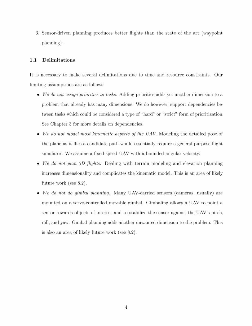
• We do not assign priorities to tasks. Adding priorities adds yet another dimension to a
problem that already has many dimensions. We do however, support dependencies be-
tween tasks which could be considered a type of “hard” or “strict” form of prioritization.
See Chapter 3 for more details on dependencies.
• We do not model most kinematic aspects of the UAV. Modeling the detailed pose of
the plane as it flies a candidate path would essentially require a general purpose flight
simulator. We assume a fixed-speed UAV with a bounded angular velocity.
• We do not plan 3D flights. Dealing with terrain modeling and elevation planning
increases dimensionality and complicates the kinematic model. This is an area of likely
future work (see 8.2).
• We do not do gimbal planning. Many UAV-carried sensors (cameras, usually) are
mounted on a servo-controlled movable gimbal. Gimbaling allows a UAV to point a
sensor towards objects of interest and to stabilize the sensor against the UAV’s pitch,
roll, and yaw. Gimbal planning adds another unwanted dimension to the problem. This
is also an area of likely future work (see 8.2).
4

Chapter 2
Related Work
In his PhD work, Morison states that sensor systems “do not provide persistent
observation without significant coordination, attentional, and cognitive costs, or guarantee
that the right sensor data will be available at the correct place and time” [13]. This problem
is central to UAVs as they are often used primarily as mobile sensor systems. Morison
proposes an approach to the problem of controlling a network of movable video cameras
using a custom input device called a “Perspective Controller.” It uses the idea of “control by
looking.” This is relevant to our work; we’d like a planner that plans based on what the user
wants to sense. This idea could be called “plan by looking,” and has been demonstrated for
fixed-wing UAVs in the context of wilderness search and rescue (WiSAR) [14].
The key to “planning by looking” is automation that can position the UAV’s sensor
in the right place at the right time. The primary constraint on sensor placement is the
directionality of the sensor; directional sensors must have line-of-sight to their targets. There
are many UAV path planning methods that could be considered. We’ll now review the
state-of-the-art in UAV path planning.
2.1 UAV Flight Planning
UAV path planning is a well-studied problem. A variety of approaches have been pursued
including A*, D*, evolutionary approaches, Rapidly-Exploring Random Trees (RRTs), Voronoi
graphs, etc. Most work has focused on the specific problem of getting a UAV from point A
to point B most efficiently, rather than planning flights that accomplish general goals. Those
5

that do plan flights to achieve a goal tend to be tailored to that specific goal and the sensors
available. We’d like a planner that can express many different goals or missions with any
kind of sensor(s).
Quigley et al. presented an A* planner meant for planning UAV flights from a start
point to an end point [15]. The planner is designed for flights in the mountains, especially
narrow canyons. The A* heuristic uses altitude change in addition to path length to avoid
unnecessary climbs. Unfortunately, the heuristic does not consider the maximum climb rate
of the UAV, so paths that climb too steeply can be generated.
Wu et al. demonstrated a D*-based planner for generating paths that comply with
civil aviation constraints on altitude, risk due to flying over populated areas, and fuel [16].
Although this approach is tailored to simply getting from a start point to an end point, its
handling of constraints besides path length is interesting.
Kothari et al. presented a real time multi-UAV planner based on RRTs that is robust
to dynamic obstacles [17]. It is a hybrid approach in that it combines RRTs with a greedy
line-of-sight strategy for “boring” stretches of flight. This planner plans flights from a start
to an end point through a field of obstacles and is not suitable for other goals.
Rathbun et al. demonstrated an evolutionary method for planning UAV paths in
dynamic, uncertain environments [18]. This method uses a genetic algorithm to plan around
dynamic obstacles with uncertain positions. The path is periodically re-planned to account
for moving obstacles. It does a good job of planning to a fixed destination from a fixed
starting point. Rathbun et al. use a spline-based representation. That is, an individual flight
is a concatenation of curves such that each successive curve starts at the ending point of the
previous curve and C1 continuity is maintained.
Building on the work by Rathbun et al. in [18], Rubio et al. presented a multi-UAV
mission planner for locating and tracking abandoned fishing nets in the Northeast Pacific
Ocean [19]. The fitness function for the evolutionary planner takes into account weather,
6
predicted icing conditions, performance degradation due to icing, and sun position. This
work is a good example of applying a UAV path planner to a non-trivial mission.
Hu and Yang presented a genetic algorithm for guiding a mobile robot through a
previously-known environment in the presence of obstacles [20]. Their genetic algorithm uses
a location-based representation. That is, an invididual is represented as a series of waypoints
in the robot’s environment. Individuals are ranked using the path’s distance and the portion
of the path that intersects obstacles.
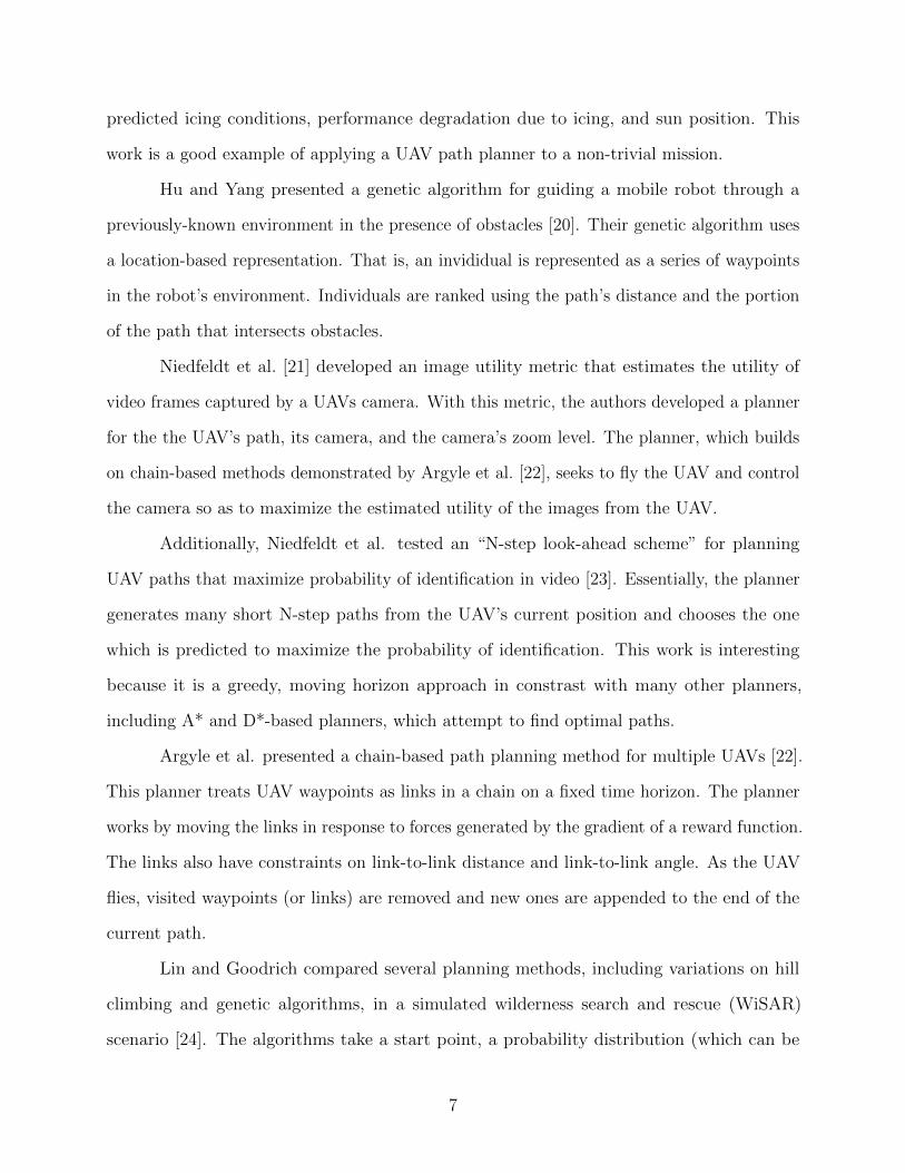
Niedfeldt et al. [21] developed an image utility metric that estimates the utility of
video frames captured by a UAVs camera. With this metric, the authors developed a planner
for the the UAV’s path, its camera, and the camera’s zoom level. The planner, which builds
on chain-based methods demonstrated by Argyle et al. [22], seeks to fly the UAV and control
the camera so as to maximize the estimated utility of the images from the UAV.
Additionally, Niedfeldt et al. tested an “N-step look-ahead scheme” for planning
UAV paths that maximize probability of identification in video [23]. Essentially, the planner
generates many short N-step paths from the UAV’s current position and chooses the one
which is predicted to maximize the probability of identification. This work is interesting
because it is a greedy, moving horizon approach in constrast with many other planners,
including A* and D*-based planners, which attempt to find optimal paths.
Argyle et al. presented a chain-based path planning method for multiple UAVs [22].
This planner treats UAV waypoints as links in a chain on a fixed time horizon. The planner
works by moving the links in response to forces generated by the gradient of a reward function.
The links also have constraints on link-to-link distance and link-to-link angle. As the UAV
flies, visited waypoints (or links) are removed and new ones are appended to the end of the
current path.
Lin and Goodrich compared several planning methods, including variations on hill
climbing and genetic algorithms, in a simulated wilderness search and rescue (WiSAR)
scenario [24]. The algorithms take a start point, a probability distribution (which can be
7

multi-modal), and an optional end point and return flight paths that take the UAV from
the start point, through the probability distribution, and to the optional end point. The
algorithms try to plan paths that take the UAV through the high-probability parts of the
distribution without visiting the same place twice.
Yang and Kapila demonstrated a distance-optimal 2D path planning method [25].
The planner takes a starting and end position, the minimum turning radius of the UAV, and
the locations and radii of obstacles. Using Dubins curves, the authors prove several geometric
theorems to justify the optimality of their planner. This work is notable because we also use
Dubins curves (or the Dubins car) as the basis of our simple kinematic model.
Bortoff proposed a two-step planner that plans for a UAV flying from a start point
to an end point through an environment of enemy radar sites [26]. The first step builds a
rough path to the destination using Voronoi polygons created around the radar sites. The
second step considers the path from step one to be a series of masses connected by springs.
The radar sites act on the masses as repulsive forces. The planner moves the masses so
as to minimize the potential energy of the system. One benefit of this method is that the
weighting of spring vs. radar forces can be adjusted to choose a desired level of “stealthiness”
or radar-avoidance.
Kaneshige and Krishnakumar described a tactical maneuvering system for aircraft
inspired by biological immune systems [27]. This interesting system generates maneuvers
that fulfill a set of requirements. e.g., “change course but keep the target in view.” Their
approach is reminiscent of evolutionary approaches like genetic algorithms. It is well-suited
to generating short maneuvers. This approach, if modified to generate long paths instead of
short maneuvers, could potentially plan flights that accomplish complex goals.
NASA’s EUROPA [28] and MAPGEN [29] provide a robust and flexible framework for
constraint-based planning. The systems were developed and used to plan missions for the Mars
rovers. MAPGEN provides “active constraint and rule enforcement,” meaning that the system
won’t allow plans which violate existing constraints to be generated. MAPGEN/EUROPA
8

use an incomplete backtracking search to complete partial mission plans. Our planning
method uses similar constraints to simplify the planning search space.
2.2 Sensor Taxonomies
There is not an overabundance of literature on categorizing UAV sensors. The categorization
that we would like, which divides sensors based on how a UAV uses them to sense a target,
does not seem to exist. There is, however, some work on more general sensor ontologies.
Russomanno et al. presented an approach to developing sensor ontologies [30]. They
also discuss problems with existing sensor ontologies and observe that: “...current computer
models of sensor ontologies are nonexistent or tend to be shallow, with only superficial aspects
of sensors expressed in taxonomies...”
White proposed a sensor classification scheme for the purposes of describing and
comparing sensors [31]. This ontology categorizes based on six aspects of sensors: measurands,
technological aspects of sensors, detection means used in sensors, sensor conversion phenomena,
sensor materials, and fields of application. While some of these aspects or dimensions are
relevant to UAV mission planning, such as measurands and technological aspects, most are
not useful for UAV planning. Sensor materials, for example, do not need to be considered
when planning for UAVs; for the purpose of path planning, whether a camera is made of
metal or plastic is not important.
9

Chapter 3
Taxonomy
Since the set of possible UAV flight plans is large and users need to be able to express
a huge variety of flights, it is necessary to come up with a small set of simple building blocks
that can describe a wide range of useful flight plans. In this section, we present a taxonomy of
sensors and tasks that serve as the basis for our general purpose sensor-driven planner. This
taxonomy is not only useful for specifying design requirements, it also enables the creation
of a hierarchical planner that uses task- and sensor-specific algorithms as needed by the
problem.
3.1 Sensors
As discussed previously, the sensors that UAVs can carry are varied. Fortunately, we can
classify them into more general canonical sensors based on how a UAV must fly in order
to use them effectively. Broadly speaking, a sensor is either directional (like a camera) or
omni-directional (like many antennas). Directional sensors need to be pointed at their target
whereas omni-directional sensors just need to be within range of it. There are, of course,
sensors that blur the distinction between directional and omni-directional, but we believe
that in such cases users can choose the classification that makes sense on a case-by-case basis.
Both sensor types are parameterized by a maximum usable distance, operationally defined
as the maximum distance at which flight tasks can be accomplished with the sensor, and a
“sensing volume.” For directional sensors, such as cameras, we can model the sensing volume
as a frustum (a flat-topped pyramid). The sensor-volumes of omni-directional sensors can
10
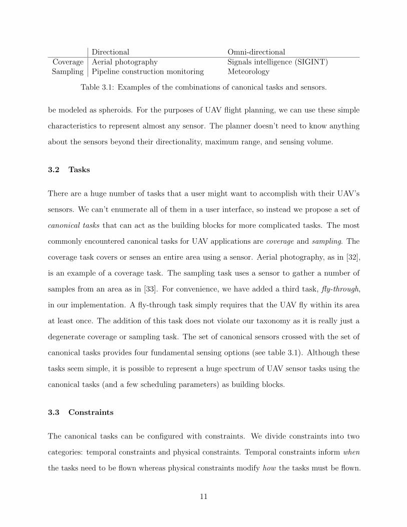
Directional Omni-directionalCoverage Aerial photography Signals intelligence (SIGINT)Sampling Pipeline construction monitoring Meteorology
Table 3.1: Examples of the combinations of canonical tasks and sensors.
be modeled as spheroids. For the purposes of UAV flight planning, we can use these simple
characteristics to represent almost any sensor. The planner doesn’t need to know anything
about the sensors beyond their directionality, maximum range, and sensing volume.
3.2 Tasks
There are a huge number of tasks that a user might want to accomplish with their UAV’s
sensors. We can’t enumerate all of them in a user interface, so instead we propose a set of
canonical tasks that can act as the building blocks for more complicated tasks. The most
commonly encountered canonical tasks for UAV applications are coverage and sampling. The
coverage task covers or senses an entire area using a sensor. Aerial photography, as in [32],
is an example of a coverage task. The sampling task uses a sensor to gather a number of
samples from an area as in [33]. For convenience, we have added a third task, fly-through,
in our implementation. A fly-through task simply requires that the UAV fly within its area
at least once. The addition of this task does not violate our taxonomy as it is really just a
degenerate coverage or sampling task. The set of canonical sensors crossed with the set of
canonical tasks provides four fundamental sensing options (see table 3.1). Although these
tasks seem simple, it is possible to represent a huge spectrum of UAV sensor tasks using the
canonical tasks (and a few scheduling parameters) as building blocks.
3.3 Constraints
The canonical tasks can be configured with constraints. We divide constraints into two
categories: temporal constraints and physical constraints. Temporal constraints inform when
the tasks need to be flown whereas physical constraints modify how the tasks must be flown.
11

There are two temporal constraints: dependencies and valid time windows. When
a task α has a dependency on task β it means that α must not be performed until β has
been performed. Valid time windows are intervals of time specified by a starting time and an
ending time with the ending time strictly greater than the starting time. A flight task must
be configured with one or more valid time windows so that it has at least one period of time
in which it can be flown.
There are also two physical constraints: orientation constraints and distance constraints.
An orientation constraint specifies that a task area must be sensed from a certain direction.
Orientation constraints specify an arc section centered on the area being sensed. An orientation
constraint could specify, for example, that a task area must be sensed when the UAV is within
45° due north of the task area. A distance constraint specifies a minimum and maximum
distance from the area being sensed. To satisfy the constraint, the UAV must be within the
range specified by the minimum and maximum distance while sensing.
3.4 Areas
There is one final building block in our taxonomy, namely the type of area. We consider two
types of areas: task areas and no-fly (obstacle or hazard) areas. Task areas should be defined
over or around areas of interest by the operator. One or more canonical tasks (e.g., coverage
or sampling) can then be assigned to the area. Alternatively, an area can be assigned as a
no-fly zone. No-fly zones are obstacles that should be avoided by the UAV. Note that in the
planner described in this thesis, areas are limited to two dimensions. Future work should
extend them to three-dimensional volumes.
3.5 Summary
In summary, the taxonomy consists of canonical tasks, canonical sensors, scheduling con-
straints, and area types. The canonical tasks are coverage and sampling. The canonical
sensor types are directional and omni-directional. Constraints include temporal constraints
12

(dependency and time window) and physical constraints (directional and distance). Areas
can be task areas (which contain one or more canonical tasks) or no-fly zones (obstacles).
We should clarify at this point that although the hierarchical planner implementation
discussed later in Chapter 5 supports all aspects of the taxonomy, the version used in
the user study doesn’t fully exploit the taxonomy since physical constraints were omitted
(see Chapter 7). With the omission of the physical constraints and our restriction to two
dimensions, there is effectively no difference between the directional and omni-directional
sensors — both sensors types are limited to sensing within some radius of the UAV’s position.
In three dimensions or in 2D with physical constraints, the distinction between sensors is
useful and dictates the way the UAV needs to fly to accomplish tasks.
Later, we will discuss how our prototype sensor-driven planner generates flights for
planning problems defined in terms of these building blocks, which can represent a variety of
UAV missions.1
1Although the taxonomy can express many UAV missions, there are limitations. It is not a good modelfor missions with task areas of non-uniform importance or with other priority schemes, for example.
13

Chapter 4
User Interface
Because users need a way to specifiy the elements of the taxonomy given in Chapter 3,
it is necessary to create a graphical user interface (GUI). A user interface is also useful for
viewing the output of the planning process.
We constructed a 2D prototype user interface using C++ and the Qt GUI toolkit (see
Figure 4.2). The GUI allows planning problems to be specified on an interactive map. The
user can define the UAV’s starting position and orientation, task areas, task’s within those
areas, and task scheduling constraints, such as dependency and time window constraints
(the means to adjust the physical constraints are not included since those constraints are
evaluated in the sub-flight algorithm comparison in Chapter 6 instead of in the user study).
No-fly zones (obstacles) can also be specified. Planning problems (encompassing the UAV’s
starting position, tasks areas, tasks, constraints, etc.) can be saved to or loaded from disk.
4.1 Dubins Curves
Dubins curves (or Dubins paths) are the shortest paths with bounded curvature connecting
two configurations (position and angle) in two-dimensional Euclidean space. L.E. Dubins
demonstrated in 1957 [34] that such curves consist solely of straight lines combined with
sections of maximum curvature.
Dubins curves provide a simple and convenient way to model 2D movement of objects
with a fixed speed and bounded angular velocity. Indeed, in the robotics and control
communities this model is often referred to as the “Dubins car” model.
14

The Dubins car model can be described with:
x = cos(θ)
y = sin(θ)
θ = u
where the position of the Dubins car is given by (x, y), its orientation (angle) is θ, and u
is bounded by the Dubins car’s minimum turning radius (or equivalently the maximum
curvature) [35]. The calculation of Dubins curves is beyond the scope of this thesis. It is
sufficient to say that there are well-studied methods of doing so [36, 37].
We use the Dubins car as an approximation for a fixed-wing UAV moving in two
dimensions. We believe that this is an acceptable approximation for the movement of fixed-
wing UAVs, which can be made to travel at a fixed speed and do in fact have bounds on
their angular velocity. Additionally, there is precedence for using Dubins curves in the UAV
planning literature [38, 39]. This model is utilized in our user interface to show the curved
path taken between two waypoints. We believe that connecting waypoints visually using
Dubins curves provides much better visual clues to the UAV’s actual performance than the
usual method of connecting waypoints using straight lines (see Figure 4.1).
We also utilize Dubins curves in the internals of the flight planner for interpolating
the configuration of the UAV between waypoints, for estimating path length, and for path
planning (see Chapter 5 for details).
4.2 Defining Planning Problems
The first element of a sensor-driven planning problem is the UAV’s initial pose, consisting
of its position and orientation. By pressing the “Place Start Point” button shown on the
left side of Figure 4.2, the user causes the starting position to be placed in the center of
the current view. The starting position is displayed in the GUI as a green circle with a line
15

Figure 4.1: Dubins curves provide a much better approximation of the actual path a fixed-wing UAV would take between waypoints than a simple straight line does. The straight linemethod would require that waysets be much more dense to approximate the same path. Webelieve that the Dubins curves provide the user with useful insight into the kinematics of theUAV.
through half of it. The position of the green circle is the starting position. The angle of the
line is the starting orientation. Once added, the starting position can be changed by clicking
and dragging the green circle around the map. The starting orientation can be changed
by right-clicking and dragging away from the green circle. The distance dragged from the
center of the green circle determines the angle of the line and therefore the UAV’s starting
orientation. In Figure 4.2, for example, the starting position is the green circle toward the
bottom-right of the map view. The starting orientation is toward the northwest.
Next, the user can add one or more task areas by pressing the “Place Task Area”
button on the left side of Figure 4.2. When pressed, this button causes a rectangular polygon
to be added at the center of the current map view. The task area is defined by the enclosed
area of this editable polygon. The user can move or delete the polygon, add or remove vertices
from the polygon, and move individual vertices (see Figure 4.3). Through these means a user
can approximate any desired area to a desired degree of accuracy. In Figure 4.2, for example,
a user has created and edited two task areas. The colors of a task area’s polygon depends on
the task(s) it contains. Coverage tasks are green, sampling tasks are blue, fly through tasks
are yellow, and no-fly zones are red. Task areas containing two or more tasks of different
types are white.
16

Figure 4.2: A screenshot of the graphical user interface (GUI). The GUI allows users to definethe elements of a sensor-driven planning problem. Task areas can be defined and edited aspolygons (see Figure 4.3) on an interactive map. The results of the planning process aredisplayed on the map.
Figure 4.3: The GUI treats task areas as editable polygons. The polygons can be translatedby clicking and dragging in their interior. Individual vertices can be translated by clickingand dragging a vertex control point. Vertices can be deleted by selecting a vertex controlpoint and pressing the “delete” key. Vertices can be inserted along any edge by clicking asubdivision point.
17

Figure 4.4: A screenshot of the GUI’s task area editor. Each task area can be configuredwith a name and zero or more sensor tasks (coverage, sampling, or fly through). Task areascan also be designated as a “no-fly zone,” or obstacle. When the “Edit” button next to atask is pressed the dialog showed in Figure 4.5 is displayed.
After a task area is defined, it can to be configured with a descriptive name, one or
more tasks, or as a no-fly zone. Users can access a dialog like that in Figure 4.4 by double
clicking a task area polygon or by right-clicking on a polygon to access a context menu entry.
The “Edit Tasks” dialog shown in Figure 4.4 allows the user to add coverage, sampling, or
fly through tasks to the area by clicking one of the buttons at the bottom. Alternatively,
the user can configure the area as a no-fly zone (obstacle). Once a task is added to the area,
its constraints and options can be configured by pressing the “Edit” button to the right of
it in the dialog. Pressing “Edit” will display a dialog similar to that shown in Figure 4.5.
Intuitively, pressing the nearby “Delete” button will remove the appropriate task from the
task area.
Individual tasks are configured in a dialog like that shown in Figure 4.5. The task can
be optionally configured with a descriptive name. Dependencies on other tasks can be added
by accessing a dropdown menu by clicking the “Add Dependency” button. Timing constraints
(time windows during which the task can be accomplished) can be added, edited, or deleted.
Finally, options specific to the task’s type (coverage, sampling, etc.) can be specified. The
18

Figure 4.5: A screenshot of the GUI’s coverage task editor. Each task type (coverage,sampling, fly through) has its own specific options as well as some (timing constraints anddependencies) that are common to all tasks.
dialog in Figure 4.5, for example, is configuring a coverage task and its task-specific options
(granularity and maximum distance) are displayed.
4.3 Planning
Once a planning problem has been defined (or loaded from disk) users can start the hierarchical
planner by pressing the “Plan Flight” button shown at the top-left of Figure 4.2. If the
hierarchical planner is successful, the generated flight is overlayed on the map and the
planning problem (see Figure 4.6). If the hierarchical planner is unable to generate a flight
that satisfies the tasks and constraints of the problem then the user is notified.
The flight is displayed as a series of waypoints strung together using Dubins curves [34].
Each waypoint has a defined longitude, latitude, and angle. The waypoints are displayed
19

Figure 4.6: The sensor-driven planning GUI displays the results of successful planningoperations as a series of Dubins curves. Planned flights can be imported and exported inseveral formats.
as arrows and the Dubins curves between them are drawn as black curves. The minimum
turning radius of the Dubins curves is set to be the same as that configured for the UAV in
the user interface. This allows the user to get a realistic idea of the actual flight that a real
UAV would fly given the series of waypoints.
After a flight is generated and displayed the user can test its performance by pressing
the “Test Flight” button on the left side of the interface or export it by pressing the “Export
Solution” button on the right side of the interface (see Figure 4.2). Flight testing is discussed
in Section 7. Flights can be exported to a custom binary format or to the XML-based GPS
Exchange Format (GPX) [40].
4.4 Alternative Planning Interfaces
Existing planning interfaces tend to be waypoint-based. That is, the user plans flights by
specifying a sequence of latitudes, longitudes, and altitudes.
Lockheed Martin Procerus Technologies develops and markets a UAV autopilot system
with an accompanying flight planning program called “Virtual Cockpit [41].” Virtual Cockpit
is representative of traditional waypoint-based planning. The interface features a map where
20

Figure 4.7: Version 2.6 of Procerus’s “Virtual Cockpit” UAV flight planner.
series of waypoints and takeoff and landing positions are displayed and configured (see
Figure 4.7). The interface also displays the in-flight status of the UAV and feeds from UAV
sensors, such as cameras.
Previous work on UAV flight planning in our lab resulted in a 3D waypoint-based
planner called “Phairwell” [14, 42]. Phairwell uses 3D graphics to display terrain loaded
from National Elevation Dataset topography data. The terrain is textured using satellite
imagery of the area (see Figure 4.8). The display of terrain in 3D helps users gain context
for the UAV’s flight and to avoid obstacles such as mountains. Phairwell is also strongly
waypoint-based, but features automated assistance for creating common flight plans such as
a “lawnmower” or a spiral search pattern.
Another project from out lab produced the user interface pictured in Figure 4.9. This
interface was part of the “2nd generation” of the HCMI lab’s WiSAR (Wilderness Search
and Rescue) software. The overall system (see Figure 4.10) was notable for using a plugin
architecture to support diverse UAV hardware and radio links. The flight planning interface,
however, features fairly simple waypoint- and map-based planning.
21

Figure 4.8: The Phairwell user UAV planning program created by the BYU HCMI lab.
Figure 4.9: Another flight system developed by the BYU HCMI lab. This system featuresUAV hardware independence and network transparency. The planning interface picturedhere is waypoint-based.
22

CommStation
Simulated UAV
Physical UAV
Piloting GUI
Video GUI
TCP/UDP
Radio or Simulated Links
Figure 4.10: Relationships between the components of the 2nd-generation WiSAR interface.
23

Chapter 5
Hierarchical Planning
The idea behind hierarchical planning is to break the planning problem into several
stages that are more tractable than the overall problem. This is necessary because generating
a flight that accomplishes all of its tasks, satisfies all of its constraints, and is optimal with
respect to flight length is quite challenging. Consider, for example, the problem posed by a
flight with n task areas, each with one assigned task to be completed. Generating a flight
that is optimal with respect to flight length and that handles all n task areas (and their
tasks) has essentially solved the traveling salesman problem by deciding the order in which
to visit the tasks [24]. In reality, since solutions to some sensor-driven planning problems can
require that tasks and task areas be revisited and we haven’t yet considered anything beyond
the ordering of the tasks, the problem is even more complex.
The taxonomy suggests that many problems can be decomposed into two sub-problems:
planning a sensor-appropriate flight path for an area/task and scheduling flight paths to
satisfy timing constraints. Therefore, the approach in this thesis breaks the problem into
pieces, plans “sub-flights” for each flight task in isolation, and then schedules the generated
flights into an overall solution. Figure 5.1 shows how the components of the hierarchical
planner generate different pieces of a flight. This chapter discusses the overall hierarchical
planning process including planning sub-flights and scheduling them into an overall flight. In
Chapter 6 we discuss and objectively compare various methods of planning sub-flights.
Broken up in this manner, the problem of flight planning closely resembles scheduling
processes on a computer. Flight tasks can be thought of as processes and the UAV can be
24

Figure 5.1: Each part of the hierarchical planner plays a different role in generating theoverall flight. In this example, C and E are sub-flights generated by the sub-flight plannerto fly tasks in the shaded areas. B and D are intermediate or connecting flights generatedby the intermediate planner, which runs as a subroutine of the scheduler. The scheduler isresponsible for deciding when to schedule sub flights. A is the UAV’s starting position.
thought of as a CPU which runs them. Just as a running process on a CPU can be preempted,
sensor-driven planning problems sometimes require a flight task to be interrupted before
completion. Just as preempting processes on a CPU has overhead, interrupting flight tasks
to handle another has the cost of travel between tasks.
The hierarchical approach has some tradeoffs and limitations. It makes the problem
tractable and the algorithm generalizable, but it sacrifices optimality in several places to do
so. One limitation with the hierarchical approach and the CPU scheduling metaphor is that
the UAV cannot fly more than one task at a time. Thus, we sacrifice optimality when flight
tasks are co-located.
At a high level, the hierarchical planner follows these easily-understood steps:
1. For each flight task:
(a) Select a task-specific starting position and orientation on or near the task area’s
boundary.
25

(b) Generate a “sub-flight” that accomplishes the flight task with its task constraints
independent of all other flight tasks. This sub-flight must start at the previously-
generated starting position and pose.
2. Generate a schedule that determines when to fly each sub-flight.
3. Using the schedule, build an overall flight by stringing the sub-flights together with
intermediate flights.
The next sections will discuss the hierarchical planner in more detail and Chapter 6 will focus
on various algorithms that attempt to plan “sub-flights.”
5.1 Task Start Position and Pose
Before the planner can generate sub-flights for each of the flight tasks, positions and orienta-
tions from which to start each sub-flight must be chosen. Choosing a good starting position
and pose is important and non-trivial. Choosing the optimal starting position and pose
(those that will result in the shortest satisfying flight) requires knowing where the UAV will
be coming from. Since the schedule isn’t computed until after all sub-flights are generated, it
is not possible to choose the optimal starting position and orientation. We can however, use
a heuristic to choose a starting position and orientation that are likely to give good results.
The goal of this heuristic (pictured in Figure 5.2) is to choose a starting position
and orientation that are close to other tasks and are likely to allow the UAV to fly for a
while without turning. This latter condition seeks to minimize path length by avoiding
potentially-costly turns, which are constrained by the rate of turning dictated by the Dubins
curves. First, we approximate the center of mass of the area by finding the center of the
area’s bounding box. We then create a set of 179 line segments that pass through the center
of mass and are one degree apart. The endpoints of the longest line segment within the task
area (which sit on edges of the task area) are examined as candidate starting positions. The
endpoint which is closest to the average of all task areas’ centers is chosen as the starting
position in an attempt to minimize the expected distance between any preceeding tasks and
26

Figure 5.2: Choosing a starting position for a task area. A bounding box is calculated aroundthe area in question. Line segments intersecting the center of the bounding box are calculatedat one degree angle intervals. The end points of the line with the most length within thearea’s polygon are candidates for the task area’s starting position. The candidate point thatis closest to the average of all task area’s bounding box centers is selected. The orientationpoints along the line.
the starting point. The starting orientation is chosen to point towards the center of mass
of the task area (i.e., the orientation follows the line segment in the direction towards the
center of mass).
5.2 Sub-Flight Planning
The sub-flight planner is the part of the hierarchical planner responsible for planning the
portions of the overall flight that accomplish tasks. The sub-flights must begin in their start
position and orientation, accomplish their tasks, and satisfy all physical constraints.
This part of the hierarchical planning process can be done a variety of different ways. In
Chapter 6 we will discuss the set of algorithms that we investigated and benchmarked during
this thesis. We found that, in general, a best-first search in a discretized location/orientation
statespace performs better than the other alternatives. See Chapter 6 for explanation and
comparison of all attempted sub-flight planners.
27

Task Type Reward Function
Coverage The task area is discretized on latitude/longitude aligned grid with spacingcontrolled by granularity parameter. Candidate sub-flights are given 1.0unit of reward for each discretized point they are able to sense with theassigned sensor type (directional or omnidirectional) within the bounds ofthe task’s physical constraints (direction and distance).
Sampling The sampling task is parameterized by s, the number of seconds thatthe sub-flight must spend within the task area. Candidate sub-flights arerewarded the amount of time spent sampling in a location that obeys thephysical constraints and limitations of the assigned sensor type.
Fly-Through Returns a fixed reward when candidate sub-flights fly within it at all. Thisis essentially a degenerae sampling or coverage task.
Table 5.1: Descriptions of the canonical tasks’ reward functions, which are used by thesub-flight planner to generate sub-flights.
One feature shared by all of the sub-flight planning algorithms we’ve examined is
that they all require reward functions for the canonical tasks. These reward functions are
summarized in Table 5.1. The reward functions are fitness functions that return a numeric
value in proportion to how well a sub-flight accomplishes a task within the bounds of the
task’s physical constraints and assigned canonical sensor type. The reward functions are used
by the sub-flight planning algorithms to generate and optimize flights. The sum of the reward
functions of all tasks in a scenario can also be used as a measure of overall flight quality.
5.3 Scheduler
Once a sub-flight has been generated for each flight task, a scheduler must decide when to fly
each one and how to string them together. Scheduling is not a trivial task due to scheduling
and dependency constraints on flight tasks.
Sometimes, one task must be interrupted to fly another due to time window constraints.
In a scenario with two tasks α and β each requiring 10 seconds to complete, for example,
task α may have the constraint that it must be completed entirely after 5 seconds but before
20 seconds (a window longer than 10 seconds is required due to the time taken to fly between
tasks). Task β would be scheduled for at least the first 5 seconds, after which a transition to
28

task α would be made. After task α is completed at around 15-20 seconds, task β would be
scheduled again and finished.
We attack the problem by returning to the CPU scheduling metaphor. Flight tasks
are processes and the UAV is a CPU. The UAV can fly a task to completion or it can run
it in time slices with other tasks, “context-switching” between them. However, flight task
scheduling has two key differences from CPU scheduling: First, we know exactly how much
time each flight task needs since sub-flights which satisfy them were calculated previously,
whereas the run time of a program cannot generally be predicted. Second, the time required to
transition or “context switch” between flight tasks is highly variable and must be considered.
We treat the scheduling problem as a graph search through an n-dimensional scheduling
space where n is the number of flight tasks in the planning problem. Our approach is inspired
by previous work in CPU and manufacturing scheduling that also uses graph search [43, 44],
although there are some key differences between those problems and ours (we know in advance
the exact durations of the task and our “context-switching” costs vary). The goal of the
search is to find a least-cost path from (01, ..., 0n) to (c1, ..., cn) where ci is the amount of
time required to complete sub-flight i. A problem of three tasks each taking 10.5 seconds, for
example, requires the scheduler to find a least-cost path from (0, 0, 0) to (10.5, 10.5, 10.5).
Note that the total time required to fly the resulting flight plan will be greater than the sum
of the sub-flights’ required times because flying transitions between tasks takes time.
Solving the scheduling problem can be done optimally (given that we are discretizing
time into fixed-size chunks) using A*. This is a good choice because we can use the estimated
time remaining from any state to the goal state as an admissible heuristic. Since the CPU
scheduling metaphor restricts the UAV to flying one sub-flight at a time, the scheduler
can only do state transitions along one dimension at a time within the scheduling space.
This means that all A* distance calculations in the scheduler, including the heuristic, use a
Manhattan rather than Euclidean distance. See Figure 5.3.
29

5,5
0,0 α
β
Task α constrained
to finish within 7
seconds.
At (3,0) the heuristic
is 7 (Manhattan
distance to goal).
Figure 5.3: The scheduling state space of an imaginary two-task planning problem. Bothtasks (α and β) take five seconds to be completed. In this example, task α has a time windowconstraint specifying that it must be finished by no later than seven seconds. Edges thatwould allow task α to make progress outside of its valid time window have been cut. The A*heuristic is Manhattan distance to the goal. Each transition in the graph corresponds to thepassing of time.
30
When the A* scheduler considers transitioning from one flight task α to another task
β it must generate a transition (or intermediate) flight from the current state’s progress along
α’s sub-flight to the generated state’s progress along β’s sub-flight. If the A* scheduler for
two tasks α and β had reached node (3,0) and wanted to explore node (3,1), for example,
it would use the intermediate planner to generate a flight from the UAV’s configuration 3
seconds into α’s sub-flight to the beginning (time 0) of β’s sub-flight. The length of the
intermediate flight is used to calculate how long it will take to transition from α to β and is
A*’s “cost to move”. Intermediate flights are stored during scheduling so that they can be
used as components of the overall flight when scheduling is completed.
Flight task scheduling constraints such as dependencies and valid time windows are
encoded in the state space as obstacles, which A* can easily deal with. Specifically, the
search is not allowed to expand into states where any task’s dependency constraints or valid
time windows are violated. It is important to note that it is very easy to create unsolvable
planning problems by creating a dependency loop among two or more tasks or by specifying
unrealistic time windows. In this situation the scheduler will search as far as it can before
detecting that the problem is overconstrained. At that point, the user is informed that the
problem is overconstrained and is invited to relax or adjust constraints.
5.4 Intermediate Planner
The intermediate planner is responsible for planning flights from the start position to task
areas and in-between task areas. Intermediate flights are planned solely to get the UAV
from one configuration to another rather than to accomplish any of the flight tasks. The
intermediate planner takes as input the positions of no-fly zones and starting and ending
positions/orientations. It outputs a series of positions or waypoints.
The requirements for the intermediate planner are challenging. First, it must be very
efficient because it runs as a subroutine of the scheduler’s A* search. Second, it must be able
to plan over long distances. Third, it must avoid no-fly zones. Finally, it has to be able to
31
plan intermediate flights that are valid according to the UAV’s kinematic constraints (the
Dubins car model) and that start and end in the correct orientations (not just positions).
Our intermediate planner, like the overall hierarchical planner, takes a hierarchical
approach. First, it builds a path using Dubins curves [34]. If this initial path does not violate
any no-fly zones then the planner has succeeded. Otherwise, the intermediate planner falls back
to using A* to generate a coarse, high-level, obstacle-avoiding path without consideration for
desired orientation or UAV kinematics. The A* search is carried out on a coarse 4-connected
graph with node spacing of 75 meters so that it will run quickly. The search is not allowed to
expand into no-fly zones. Next, it strings the nodes of the A* search together using Dubins
curves [34], which ensure that the desired starting and ending orientations are honored and
that UAV kinematic constraints are obeyed. Future work should explore how the subjective
granularity parameters used in the A* planner would need to be adjusted for different types
of planning problems, e.g., those that span tens or hundreds of kilometers instead of only a
few kilometers.
5.5 Performance Considerations
The performance of the hierarchical planner depends on several factors. In order of importance
these are the number of tasks, the duration of the tasks, timing constraints and dependencies,
and the relative locations of tasks and obstacles. The number of tasks is the largest factor
because it is also the dimensionality of the scheduler’s search space (see Section 5.3). When
generating a flight plan for a problem with three tasks, for example, the scheduler must
search a three-dimensional space. As can be expected, the scheduling space for a problem
with twenty tasks is very large.
There are several simple techniques for shrinking or pruning the scheduler’s statespace.
First and foremost, the user can add more scheduling constraints. As discussed in 5.3, the
result of dependency and timing constraints is cut edges in the scheduling graph. This is
akin to adding more information to an under-determined mathematical formula; the number
32

of possible solutions greatly decreases. Second, for scenarios with no time window constraints
the scheduler can forbid task interruption. That is, the scheduler prunes edges that transition
from a task that has not yet been scheduled to completion. This “interruption optimization”
is acceptable since there is little reason to consider interrupting a task α unless some task
β must be scheduled immediately based on a timing constraint. However, the optimization
may cause suboptimal performance on some edge cases (e.g., a small task area adjacent to a
very large task area). Third, the time-granularity of the scheduler (the duration of the “time
chunks” that the scheduler works with) can be increased. This can result in the scheduler
failing to find solutions for problems which are schedulable with smaller “time chunks,” or
finding a less efficient schedule. Finally, the A* heuristic can be multiplied by some weight
w : w ∈ (1,∞) as in Weighted A* [45]. This has the effect of emphasizing the estimated
“cost-to-move” vs. the cost already incurred, which encourages Weighted A* to find a (likely
sub-optimal) solution more quickly than normal A* can find the optimal solution. Weighted
A* has the useful guarantee that the cost of solutions must be within a factor of w of the
optimal solution’s cost [46].
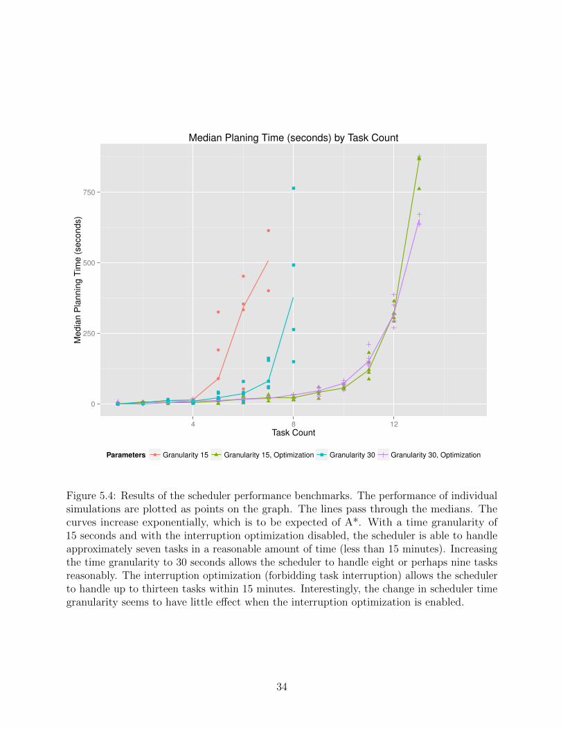
We benchmarked the scheduler’s performance on randomly-generated scenarios with
number of tasks ranging from 1-13. The generated task areas were rectangular with widths
and heights drawn uniformly from [300, 350] meters. Each task area was assigned with equal
probability as either a coverage, sampling, or fly-through task. The placement of task areas
was constrained to be non-overlapping. We tested two of the optimizations listed above:
increasing the scheduler granularity and forbidding task interruption. The scheduler was
given 900 seconds (15 minutes) to schedule each scenario. The results of the benchmarks are
summarized in Figure 5.4.
The results of the benchmarks indicate that without scheduling constraints or optimiza-
tions the scheduler can reasonably handle five or six tasks. Increasing the time granularity to
30 seconds allows a slight improvement to seven or eight tasks. Enabling the interruption
optimization (forbidding task interruption) results in a large speed-up, enabling the scheduler
33
●●●●● ●●●●●●●●●● ●●●
●●
●
●
●●
●
●
●
●
●
●
●
0
250
500
750
4 8 12
Task Count
Media
n P
lannin
g T
ime (
seconds)
Parameters ● Granularity 15 Granularity 15, Optimization Granularity 30 Granularity 30, Optimization
Median Planing Time (seconds) by Task Count
Figure 5.4: Results of the scheduler performance benchmarks. The performance of individualsimulations are plotted as points on the graph. The lines pass through the medians. Thecurves increase exponentially, which is to be expected of A*. With a time granularity of15 seconds and with the interruption optimization disabled, the scheduler is able to handleapproximately seven tasks in a reasonable amount of time (less than 15 minutes). Increasingthe time granularity to 30 seconds allows the scheduler to handle eight or perhaps nine tasksreasonably. The interruption optimization (forbidding task interruption) allows the schedulerto handle up to thirteen tasks within 15 minutes. Interestingly, the change in scheduler timegranularity seems to have little effect when the interruption optimization is enabled.
34

Figure 5.5: A contrived scenario with fifteen tasks, all but two of which depend on anothertask such that no task depends on the same task as another and there are no cycles in thedependency graph. The A* scheduler completed this scenario in approximately four seconds.
to handle twelve or thirteen tasks in under fifteen minutes. We believe that the pair of curves
without the interruption optimization represent the worst-case scenario for the scheduler:
several tasks with no temporal constraints to prune the statespace. Perhaps, then, the pair
of curves generated with the interruption optimization enabled represent a more optimistic
scenario with a few temporal constraints. The far end of the optimism spectrum is represented
by the contrived scenario pictured in Figure 5.5, which has thirteen dependency constraints
and can be scheduled in approximately four seconds.
The scenarios used in the user study (see Figures A.1, A.2, A.3, and A.4) each contain
four tasks and are moderately constrainted (they have a couple timing and dependency
constraints). The scheduler is able to complete them in about 5-10 seconds with a time
granularity of 15 seconds.
In summary, the performance of the scheduler varies. When tasks are unconstrained
the scheduler can cope with 6-8 moderately-sized tasks. Temporal constraints allow the
scheduler to handle more tasks. In a contrived scenario (see Figure 5.5) with fifteen tasks
35

and thirteen dependency constraints, for example, the scheduler completes in approximately
four seconds. Without temporal constraints, a scenario with fifteen tasks is unlikely to be
schedulable in a reasonable amount of time. We believe that real-world users are likely to
add temporal (dependency or time window) constraints to their scenarios and that most
real-world scenarios do not require many tasks. Therefore, we believe that the scheduler’s
performance is likely to be adequate.
36

Chapter 6
Sub-Flight Planning
In this section we compare and benchmark various sub-flight planning algorithms.
Based on the analysis, we show that a best-first search in a discretized position/orientation
statespace performs well. First, we discuss the discretized position/orientation statespace,
which is used by several of the algorithms in this chapter. Then, we describe the various
sub-flight planning algorithms. Finally, we present the results of benchmarks of the algorithms’
performance.
6.1 Discretized Position/Orientation Statespace
Several of the sub-flight planning algorithms described in this section operate in a statespace
based on a grid of positions and a set of valid UAV orientations at those positions. We refer
to this as a position/orientation statespace.
Calculating this statespace is simple. First, positions are generated by discretizing
(calculating a grid within) the task area polygon’s bounding box. Second, all positions which
are not inside of the task area polygon are eliminated. Next, the positions are translated in
the direction of the task’s directional constraint (if any) by the task’s distance constraint
(if any). Finally, a set of valid orientation angles are calculated at the translated positions
based on the directional constraint of the task and the directional sensor’s angle-of-view (if
applicable). If, for example, a task’s directional constraint stipulates that it must be sensed
from the south (270°), then the calculated orientations will point roughly north (90°), within
the bounds of the directional sensor’s angle-of-view, if applicable (see Figure 6.1).
37

Directional constraintcauses translation to the south.
Caluclated orientationspoint north so that aUAV's directional sensorwould be able to sense the task area.
Figure 6.1: Calculating the position/orientation space requires translating discretized pointswithin the task area by a distance no less than the minimum distance constraint in thedirection of the directional constraint. If the task is configured to be sensed using a directionalsensor, then the translated points must be assigned orientations. This process yields a setof positions and orientations which are guaranteed to conform to the physical (directionaland distance) constraints when flown by the UAV. Sub-flight planning algorithms can searchthrough the transformed set without worrying about the physical constraints. This figureillustrates a pentagonal task area whose discretized points have been translated to the southto conform to a distance constraint. The points have been assigned north-facing orientationsfor directional sensing.
38

A sequence of these position/orientation pairs can always be combined into a kinematically-
viable sub-flight using Dubins curves provided that the distance between successive positions
is greater than zero.
6.2 Best-First Tree Search
The best-first tree search sub-flight planner searches a tree with nodes defined by a position
and a pose. The root node, for example, is the task area’s starting position and pose. The
search generates child nodes by making valid moves (according to the UAV’s kinematic
constraints) from the best current node. Each task type (sampling, coverage, etc.) defines a
reward function (see Table 5.1) that rates prospective sub-flights, which are represented by
the position and poses of the nodes from root to leaf.
At each iteration the node with the highest reward is removed from a work list. New
orientation vectors are calculated based on the current node’s orientation and the UAV’s
kinematic parameters. In addition, new positions are generated by translating the current
node’s position by each of the previously generated angles. New nodes are created as children
of the current node with the generated orientations and positions. Score values are generated
for the new nodes using the flight task’s reward function and the new nodes are inserted into
the work list. This process is summarized in Algorithm 1.
6.3 Best-First Search in Discretized Position/Orientation Statespace
This algorithm is similar to that of the best-first tree search described above (see 6.2) except
that, instead of limiting transitions based on kinematic constraints, all locations in the
discretized statespace described in 6.1 are considered for transitions. The series of nodes
representing a sub-flight in this planner are combined using Dubins curves to ensure kinematic
viability. See Algorithm 2 for details.
39
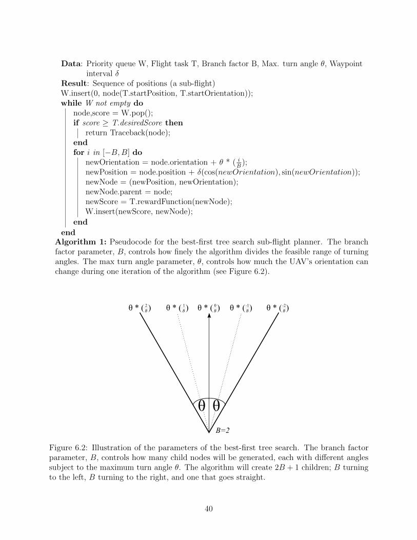
Data: Priority queue W, Flight task T, Branch factor B, Max. turn angle θ, Waypointinterval δ
Result: Sequence of positions (a sub-flight)W.insert(0, node(T.startPosition, T.startOrientation));while W not empty do
node,score = W.pop();if score ≥ T.desiredScore then
return Traceback(node);endfor i in [−B,B] do
newOrientation = node.orientation + θ * ( iB
);newPosition = node.position + δ(cos(newOrientation), sin(newOrientation));newNode = (newPosition, newOrientation);newNode.parent = node;newScore = T.rewardFunction(newNode);W.insert(newScore, newNode);
end
endAlgorithm 1: Pseudocode for the best-first tree search sub-flight planner. The branchfactor parameter, B, controls how finely the algorithm divides the feasible range of turningangles. The max turn angle parameter, θ, controls how much the UAV’s orientation canchange during one iteration of the algorithm (see Figure 6.2).
θθ
θ * ( )-1B
θ * ( )-2B
θ * ( )0B
θ * ( ) 1B
θ * ( )2B
B=2
Figure 6.2: Illustration of the parameters of the best-first tree search. The branch factorparameter, B, controls how many child nodes will be generated, each with different anglessubject to the maximum turn angle θ. The algorithm will create 2B + 1 children; B turningto the left, B turning to the right, and one that goes straight.
40
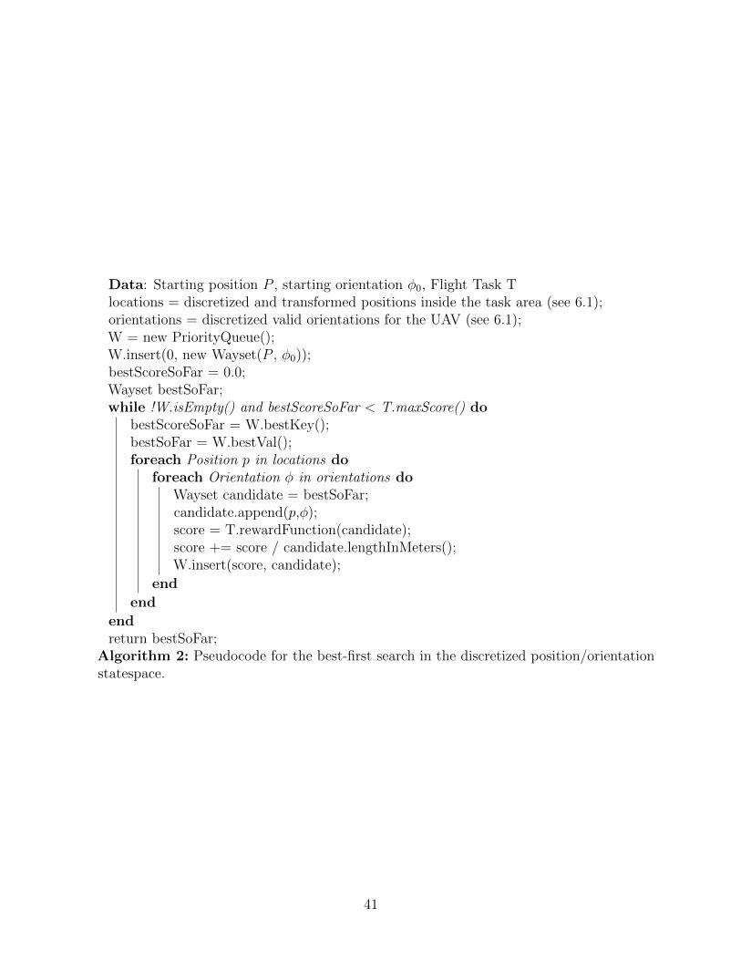
Data: Starting position P , starting orientation φ0, Flight Task Tlocations = discretized and transformed positions inside the task area (see 6.1);orientations = discretized valid orientations for the UAV (see 6.1);W = new PriorityQueue();W.insert(0, new Wayset(P , φ0));bestScoreSoFar = 0.0;Wayset bestSoFar;while !W.isEmpty() and bestScoreSoFar < T.maxScore() do
bestScoreSoFar = W.bestKey();bestSoFar = W.bestVal();foreach Position p in locations do
foreach Orientation φ in orientations doWayset candidate = bestSoFar;candidate.append(p,φ);score = T.rewardFunction(candidate);score += score / candidate.lengthInMeters();W.insert(score, candidate);
end
end
endreturn bestSoFar;
Algorithm 2: Pseudocode for the best-first search in the discretized position/orientationstatespace.
41

6.4 Genetic Algorithm in Discretized Position/Orientation Statespace
A genetic algorithm can be used to find a sequence of position/orientation pairs that, when
combined using Dubins curves, make a good sub-flight. The “genome” for individuals in
this genetic algorithm is simply a sequence of position/orientation pairs. Generations of
individuals are created, evaluated, and bred in a loop until a viable sub-flight is generated. By
default, each individuals’s genome length is the number of positions in the position/orientation
statespace (this is a good default for coverage tasks which will want to visit each position)
but as individuals are bred together this number can increase or decrease. See Algorithm 3
for details.
In our testing the genetic algorithm used a generation size of twenty. Of the twenty
individuals in each generation, half (ten) are culled. To bring the count back to twenty,
eight new individuals are bred from the ten survivors and two new “mutant” individuals are
generated randomly (to ensure genetic diversity). These parameters were chosen subjectively.
We believe that a survival rate of one-half strikes a good balance between removing bad
individuals and keeping diversity in the “gene pool.” Similarly, our 4:1 breed-to-mutate ratio
was chosen to strike a balance between taking advantage of the best-scoring individuals and
searching new parts of the space.
6.5 Simple Greedy Search in Discretized Position/Orientation Statespace
This method greedily builds a flight by choosing the best option at each step. In constrast to
the best-first methods discussed above, it does not use a work list or priority queue. Once
this method travels down a branch the decision is permanent. See Algorithm 4 for details.
6.6 Comparison
Based on the four combinations of {Coverage, Sampling} × {Directional,Omnidirectional},
we constructed four simple one-task scenarios, each with easy and hard parameter settings
42

Data: Starting position P , starting orientation φ0, Flight Task Tlocations = discretized and transformed positions inside the task area (see 6.1);orientations = discretized valid orientations for the UAV (see 6.1);bestScore = 0.0;Wayset bestFlight;W = new PriorityQueue();while bestScore < T.maxScore() do
while W.size() < 20 doWayset candidate;candidate.append(P ,φ0);for 0 ≤ i < locations.size() do
candidate.append(locations[randInt() % locations.size()],orientations[randInt() % orientations.size()]);
endscore = T.rewardFunction(candidate);score += score / candidate.lengthInMeters();W.insert(score, candidate);
endbestScore = W.bestKey();bestFlight = W.bestVal();for 0 ≤ i < 10 do
W.removeWorst();endfor 0 ≤ i < 8 do
Wayset A = W.randomValue();Wayset B = W.randomValue();startA = randInt() % A.size();endA = startA + randInt() % (A.size() - startA);startB = randInt() % B.size();endB = startB + randInt() % (B.size() - startB);Wayset candidate;candidate.append(P ,Θ);for startA ≤ j < endA do
candidate.append(A[j]);endfor startB ≤ j < endB do
candidate.append(B[j]);endscore = T.rewardFunction(candidate);score += score / candidate.lengthInMeters();W.insert(score, candidate);
end
endreturn W.bestVal();
Algorithm 3: Pseudocode for the best-first search in the discretized position/orientationstatespace.
43

Data: Starting position P , starting orientation φ0, Flight Task Tlocations = discretized and transformed positions inside the task area (see 6.1);orientations = discretized valid orientations for the UAV (see 6.1);Wayset current;current.append(P ,φ0);bestScore -500.0;while !locations.isEmpty() and bestScore < T.maxScore() do
bestScore = -500.0;bestBinIndex = -1;UAVOrientation bestOrientation;for 0 ≤ i < locations.size() do
Position pos = locations[i];Wayset toTest = current;foreach approachAngle in orientations do
toTest.append(pos, approachAngle);score = T.rewardFunction(toTest);if score > bestScore then
bestScore = score;bestOrientation = approachAngle;bestBinIndex = i;
end
end
endPosition toAdd = locations[bestBinIndex];current.append(toAdd,bestOrientation);
endreturn current;
Algorithm 4: Pseudocode for the greedy search in the discretized position/orientationstatespace.
44
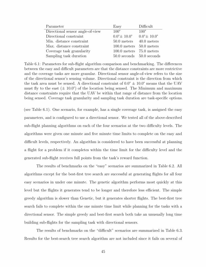
Parameter Easy DifficultDirectional sensor angle-of-view 100° 100°Directional constraint 0.0°± 10.0° 0.0°± 10.0°Min. distance constraint 50.0 meters 40.0 metersMax. distance constraint 100.0 meters 50.0 metersCoverage task granularity 100.0 meters 75.0 metersSampling task duration 50.0 seconds 50.0 seconds
Table 6.1: Parameters for sub-flight algorithm comparison and benchmarking. The differencesbetween the easy and difficult parameters are that the distance constraints are more restrictiveand the coverage tasks are more granular. Directional sensor angle-of-view refers to the sizeof the directional sensor’s sensing volume. Directional constraint is the direction from whichthe task area must be sensed. A directional constraint of 0.0° ± 10.0° means that the UAVmust fly to the east (± 10.0°) of the location being sensed. The Minimum and maximumdistance constraints require that the UAV be within that range of distance from the locationbeing sensed. Coverage task granularity and sampling task duration are task-specific options.
(see Table 6.1). One scenario, for example, has a single coverage task, is assigned the easy
parameters, and is configured to use a directional sensor. We tested all of the above-described
sub-flight planning algorithms on each of the four scenarios at the two difficulty levels. The
algorithms were given one minute and five minute time limits to complete on the easy and
difficult levels, respectively. An algorithm is considered to have been successful at planning
a flight for a problem if it completes within the time limit for the difficulty level and the
generated sub-flight receives full points from the task’s reward function.
The results of benchmarks on the “easy” scenarios are summarized in Table 6.2. All
algorithms except for the best-first tree search are successful at generating flights for all four
easy scenarios in under one minute. The genetic algorithm performs most quickly at this
level but the flights it generates tend to be longer and therefore less efficient. The simple
greedy algorithm is slower than Genetic, but it generates shorter flights. The best-first tree
search fails to complete within the one minute time limit while planning for the tasks with a
directional sensor. The simple greedy and best-first search both take an unusually long time
building sub-flights for the sampling task with directional sensors.
The results of benchmarks on the “difficult” scenarios are summarized in Table 6.3.
Results for the best-search tree search algorithm are not included since it fails on several of
45

Algorithm Task Sensor Success Planning Time Flight LengthGenetic Coverage Directional TRUE 2.01 s 6.02 kmGenetic Coverage Omnidirectional TRUE 0.68 s 3.43 kmGenetic Sampling Directional TRUE 7.64 s 4.53 kmGenetic Sampling Omnidirectional TRUE 6.75 s 2.20 kmSimple Greedy Coverage Directional TRUE 1.02 s 3.51 kmSimple Greedy Coverage Omnidirectional TRUE 1.45 s 2.07 kmSimple Greedy Sampling Directional TRUE 40.88 s 3.89 kmSimple Greedy Sampling Omnidirectional TRUE 3.32 s 1.23 kmBest-First Tree Coverage Directional FALSEBest-First Tree Coverage Omnidirectional TRUE 5.33 s 1.62 kmBest-First Tree Sampling Directional FALSEBest-First Tree Sampling Omnidirectional TRUE 5.13 s 1.14 kmBest-First Coverage Directional TRUE 0.67 s 1.90 kmBest-First Coverage Omnidirectional TRUE 1.10 s 1.43 kmBest-First Sampling Directional TRUE 20.60 s 2.71 kmBest-First Sampling Omnidirectional TRUE 5.55 s 1.02 km
Table 6.2: Results of sub-flight comparison on the “easy” scenarios. The best results for eachtask/sensor combination are bolded.
the easy scenarios. The simple greedy algorithm fails to finish (within the five-minute time
limit) the sampling task with a directional sensor. The genetic and best-first algorithms are
able to complete all the difficult scenarios within the allotted time limit. However, best-first
takes a lot of time on the sampling tasks. There seems to be a tradeoff between the genetic
and best-first algorithms. Genetic is very quick to find an inefficient solution. Best-first takes
longer, but generates more efficient sub-flights. There is an exception with the Directional
sampling task, where the genetic algorithm is able to find a shorter flight than best-first does.
Of all the sub-flight algorithms we tested, only two, genetic and best-first, are able to
successfully plan sub-flights for the easy and difficult scenarios. Restricting the analysis to
these two algorithms, it can be seen that there is a tradeoff between computation time and
minimization of flight length, or efficiency (see Figure 6.3). The choice of which algorithm
to use in practice can be made on a case-by-case basis based on the relative importance of
computation time and flight efficiency. We believe that in most cases, the best-first method
is preferable by virtue of it generating much shorter flights.
46

Algorithm Task Sensor Success Planning Time Flight LengthGenetic Coverage Directional TRUE 38.49 s 19.18 kmGenetic Coverage Omnidirectional TRUE 39.70 s 13.06 kmGenetic Sampling Directional TRUE 9.47 s 1.11 kmGenetic Sampling Omnidirectional TRUE 8.29 s 10.58 kmSimple Greedy Coverage Directional TRUE 12.74 s 6.77 kmSimple Greedy Coverage Omnidirectional TRUE 15.49 s 3.85 kmSimple Greedy Sampling Directional FALSESimple Greedy Sampling Omnidirectional TRUE 141.70 s 5.53 kmBest-First Coverage Directional TRUE 9.93 s 4.52 kmBest-First Coverage Omnidirectional TRUE 27.80 s 3.59 kmBest-First Sampling Directional TRUE 258.98 s 7.92 kmBest-First Sampling Omnidirectional TRUE 103.96 s 4.56 km
Table 6.3: Results of sub-flight comparison on the “difficult” scenarios. The best results foreach task/sensor combination are bolded. Results for the best-first tree search algorithm arenot included for the difficult scenarios since it fails to complete all easy scenarios.
Best−First Genetic
51
015
Length of Sub−flight (kilometers) by Planner
Best−First Genetic
050
10
0150
200
250
Time−to−Plan (seconds) by Planner
Figure 6.3: Boxplots comparing the runtime and solution length of the genetic and best-firstsub-flight planning algorithms on the “difficult” scenarios. The best-first method often takeslonger to plan than the genetic planner, but nearly always produces a much shorter flight.
47

Chapter 7
User Study
In order to validate our claims or hypotheses (see Chapter 1) it is necessary to conduct
a user study. The claim that sensor-driven planning can be used by non-expert users simply
required that we conduct an experiment where non-experts use the graphical user interface to
plan some flights. The claims that sensor-driven planning is easier to use and creates better
flights, however, required a comparison with the state of the art. Since waypoint planning is
currently the most common method of UAV flight planning, we constructed a simple but
adequate waypoint-based planning interface, which will be discussed in Section 7.2.
We should clarify that the 2D hierarchical planner used for the user study is a
“stripped down” version that does not include the physical constraints. Excluding the physical
constraints from the user study simplified user training, allowed each participant to finish in
a reasonable amount of time, and simplified the statistical design of the study.
We created four scenarios with which to test both planning methods (sensor-driven
and waypoint-based). Each scenario utilizes every feature of the planning taxonomy 1 —
coverage, sampling, and fly through tasks, dependency and timing constraints, and obstacles
(see Table 7.1). However, two of the four scenarios emphasize coverage tasks whereas the
other two emphasize sampling tasks. Each scenario includes a briefing document that users
can reference before and during the planning process. The briefings contain a map of the
vicinity, approximate outlines of the task areas (and obstacles) of interest, a written summary
of the tasks and constraints required, and a wilderness search and rescue-inspired “story” to
motivate the scenario and for ecological validity. An example briefing document is shown in
1With the above-noted exception of the physical constraints.
48

ScenariosTaxonomy Elements A B C D
Coverage Task(s) 2 1 2 1Sampling Task(s) 1 2 1 2
Fly-Through Task(s) 1 1 1 1No-Fly Zone(s) 1 1 1 1
Dependency Constraint(s) 4 1 3 6Timing Constraint(s) 1 1 1 1
Table 7.1: A summary of the four scenarios and the elements of the taxonomy that eachfeatures.
Figure 7.1 and the other briefing documents are given in Appendix A. The task areas shown
in the briefings are coarse so that users are forced to draw their own rectangles based on the
contents of the briefing rather than copying the areas that are shown.
Since we have two planning methods to compare (sensor-driven and waypoint-based),
four scenarios in which to test them, and we test all users on each planning method, our
experiment is a 2x4 within-subjects experiment. To minimize the potential negative effects
of a within-subjects design (effects due to fatigue and learning/practice), we counterbalance
users’ exposure to the sensor-driven and waypoint-based planning techniques. The order in
which scenarios are performed and the planning method used are also counterbalanced (see
Table 7.2). The scenarios are designed in such a way that A is comparable in difficulty to C
and B is comparable to D. This allows us to always group A with B and C with D in the
counterbalancing permutations, which reduces the number of permutations required.
7.1 Secondary Task
During each scenario with either planner, the users are required to manage a secondary
task. Our secondary task takes the form of simulated text-based commications (chat) with
a wilderness search and rescue (WiSAR) team. Users are required to monitor the chat for
messages from the WiSAR “incident commander” (the leader in a search and rescue situation),
each of which requires that the user respond with a two-digit numeric response code. Users
have to monitor the chat for messages from the incident commander, which are dispersed
49

A - Midway
NOTES
● Field
○ Must be completed before River
● South River
○ Must be completed during the time window 300 - 620 seconds.
○ Must be sampled for at least 30 seconds.
● Landing Zone
○ Must be completed last
● Do not fly over the spiral hill!
DETAILS
Yesterday morning a thirteen year-old boy left home to walk to the River to go fishing. The river is in early spring
flood stage and his family has not heard or seen him since. Search and Rescue was called in last night. The boy
often cut through the large circular Field, which is marked on your map, on his way to the River.
We need a flight plan to gather complete photo coverage of the circular field and the boy’s usual fishing ground. In
addition, we’d like to gather photo samples of the marked South River area in case any evidence of the boy’s
passing has been washed downstream. Your flight plan should start at the marked position (near the family’s home).
In order to conserve fuel, be sure to not fly over the large hill.
Figure 7.1: An example briefing document from the user study. The briefings featured a mapof the overall area annotated with areas of interest (task areas). The annotations are donevery coarsely, as if drawn by hand on a paper map. This forces users to create their owntask areas based on context rather than copying the ones in the briefing. It also helps set themood of an actual search scenario (ecological validity).
50

A1 B1 C2 D2C1 D1 A2 B2C2 D2 A1 B1A2 B2 C1 D1
B1 A1 D2 C2D1 C1 B2 A2D2 C2 B1 A1B2 A2 D1 C1
A1 B1 D2 C2C1 D1 B2 A2C2 D2 B1 A1A2 B2 D1 C1
B1 A1 C2 D2D1 C1 A2 B2D2 C2 A1 B1B2 A2 C1 D1
Table 7.2: We use sixteen different permutations of experiment order to provide counterbal-ancing. Since scenarios A and B are roughly equivalent to scenarios B and D we can alwaysgroup A with B and C with D. Otherwise, all other permutations are considered.
among other distracting and unimportant messages from other simulated members of the
WiSAR team.
The frequency of messages, both the important incident commander messages and
the distracting messages, is modeled using normal distributions. The frequency between each
incident commander message is drawn from a normal distribution with µ = 15 seconds and
σ = 13 seconds. The frequency between each distractor message was drawn from a normal
with µ = 7.5 seconds and σ = 5.5 seconds. The program discards and re-draws in the case of
drawing a negative number. These parameters were chosen by trial and error so that the
secondary task was neither too easy nor too difficult and so that the incident commander
messages are relatively rare compared to the distracting messages.
During each scenario, users’ performance on the secondary task is recorded. Specifically,
we record the time between incident commander messages and users’ correct responses
(latency) and the ratio of good responses to missed/invalid responses. As a reminder to
the users and to incentivize them, color-coded statistics about secondary task performance
51

Figure 7.2: A screenshot of the secondary task (a simulated chat with a search and rescueteam) for the user study. The interface displays statistics about users’ performance on thechat to incentivize them.
are displayed below the chat display and the outgoing chat line entry. When a user does
not respond to an incident commander message before a new one is generated, a “missed
responses” counter (see Figure 7.2) is incremented and flashes red. Correct responses cause
a “good responses” counter to increment and flash green. The user’s response rate (%) and
average response latency are highlighted green when they are doing well, yellow when they
are performing marginally, and red when they are performing poorly.
The secondary task chat display can be seen at the bottom of the sensor-driven
planning GUI in Figure 4.2, at the bottom of the comparison waypoint-based interface in
Figure 7.3, and close-up in Figure 7.2.
7.2 Waypoint Planner
A screenshot of the waypoint planner is shown in Figure 7.3. We developed the waypoint
planner with the goal of keeping as much functionality in common with the sensor-driven
planner as possible, both to save development effort and to minimize differences between the
two besides the planning method used (sensor-driven vs. waypoint-based). The waypoint
planner has the same map display and secondary task display as the sensor-driven planner.
52

The location, appearance, and functionality of common buttons such as “Export Flight”,
“Import Flight”, “Reset,” and ”Exit” are the same.
The waypoint interface allows user to create and edit a series of waypoints. Waypoints
can be appended, inserted, deleted, and moved. The waypoints are connected using Dubins
curves which give the user a good idea of where an idealized fixed-wing UAV with a bounded
angular velocity and fixed speed would actually fly. The angle of each waypoint is an average
of the angles to the previous and next waypoint weighted (or linearly interpolated) by the
distance to them, respectively. The interface also features a timeline which shows how long
(from the beginning of flight) a UAV would take to reach each waypoint at a configured speed.
7.3 Flight Testing
It is necessary during the experiments for users to be able to test the flights they generate
(using either planning method) to ensure that they accomplish the tasks and satisfy the
constraints of the scenarios. This enables users to receive feedback on their performance and
helps us to measure flight quality.
The sensor-driven planner and the waypoint-based comparison planner both have a
“Test Flight” button that users can use to verify that the flights they generate accomplish the
tasks and satisfy the constraints of the scenario. Since each scenario is defined as a planning
problem, the planners can load them as needed for flight testing. The scenarios loaded into
the planning interfaces are loaded into the background only for testing. That is, the task
area polygons defined in the scenario are not displayed. This is to ensure that users have to
create their own polygons or waypoints based on the scenario briefing.
The flight test functionality assigns a score to the user’s discretized flight by summing
up the scores returned by the sub-flights’ reward functions (see Table 5.1). In addition to
performance on the sub-flights, the flight tester evaluates compliance with dependencies,
timing constraints, and no-fly zones. The flight score is reported to the user (as a percentage
53
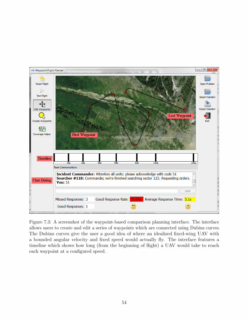
Figure 7.3: A screenshot of the waypoint-based comparison planning interface. The interfaceallows users to create and edit a series of waypoints which are connected using Dubins curves.The Dubins curves give the user a good idea of where an idealized fixed-wing UAV witha bounded angular velocity and fixed speed would actually fly. The interface features atimeline which shows how long (from the beginning of flight) a UAV would take to reacheach waypoint at a configured speed.
54

of possible performance) along with the number of dependency, timing constraint, and no-fly
violations.
7.4 Measurements and Procedures
In this section we discuss the procedure used for each user study participant as well as the
information that we collect at each stage. Figure 7.4 summarizes the experiment procedure
for sequence A1—B1—C2—D2.
First, users are instructed to read and sign an institution review board-approved
consent form. Next, users are instructed to sit at a computer and are given a general verbal
introduction and some general verbal instructions.
When a user is ready, the automated user study sequence is started. The user is
presented with a pre-user study survey, the purpose of which is to obtain general demographic
information such as gender and age (see Figure A.8). Next, the user is shown a video that
introduces the general concept of UAV flight planning and experiment procedures common to
both planning methods, such as the secondary (chat) task. After the introduction video, the
user is shown a training video for the first planning interface in their experiment sequence
(see Table 7.2)
Next, the user is given a practice scenario and an opportunity to practice the first
planning interface on the practice scenario. The practice scenarios are similar to the full
scenarios discussed in Table 7.1, but are less complicated and easier. During the practice
scenarios (and the real scenarios) we record the time taken to plan, secondary task performance
(response rate and latency), number of mouse clicks, and the performance of each flight
generated (task performance and scheduling constraint violations). Users are instructed to
plan until they are satisfied with the performance of their flight as measured by the “flight
test” functionality discussed in section 7.3. When they are satisfied, they simply exit the
planning interface to proceed to the next step.
55

1. Take pre-survey2. View introduction video3. View training video for planning interface 14. Practice with planning interface 1
(a) View briefing for practice scenario(b) Perform practice scenario with planning interface 1
5. A1(a) View briefing for scenario A(b) Perform scenario A with planning interface 1(c) Take NASA-TLX survey for A1
6. B1(a) View briefing for scenario B(b) Perform scenario B with planning interface 1(c) Take NASA-TLX survey for B1
7. Take a break8. View training video for planning inerface 29. Practice with planning interface 2
(a) View briefing for practice scenario(b) Perform practice scenario with planning interface 2
10. C2(a) View briefing for scenario C(b) Perform scenario C with planning interface 2(c) Take NASA-TLX survey for C2
11. D2(a) View briefing for scenario D(b) Perform scenario D with planning interface 2(c) Take NASA-TLX survey for D2
12. Take post-survey
Figure 7.4: User study procedure for experiment sequence A1—B1—C2—D2.
56

After the practice scenario for the first planning interface the experiment proceeds
to the two scenarios (A and B or B and D) for the first planning interface. After each
scenario, users are asked to rank task difficulty using a web-based implementation of NASA-
TLX [47] (see Figure A.7). NASA-TLX, or the NASA Task Load Index, is a well-studied
and accepted way of measuring workload using a survey of six dimensions (mental, physical,
temporal, performance, effort, and frustration) on a 100-point scale. Normally, users perform
a pairwise comparison between the dimensions to produce a weight for each of the dimensions,
which are used to combine them into an overall score on a 100-point scale. We do not have
users perform the normal pairwise comparison between dimensions to generate weights. We
found that this process confuses and frustrates users and takes too much time during the user
study. Instead, we sum the dimensions’ sub-scores to arrive at an overall score on a 600-point
scale, a variation referred to as “raw TLX” [48]). Because the secondary task acts as another
way to measure workload, correlations between raw TLX and secondary task performance
allow us to determine if any differences are the result of actual workload or rather an artifact
of using raw TLX.
When a user has completed the first two non-practice scenarios with the first planning
interface they are given the opportunity to take a break to use the restroom, walk around,
etc. When the user is ready to proceed, they are shown a training video for the second
planning interface of their experiment sequence and given the opportunity to practice with
it on another practice scenario. After the practice, they perform the last two non-practice
scenarios (with accompanying NASA-TLX surveys).
After all scenarios have been completed users are asked to complete a post-survey.
The purpose of the post-survey is to gather subjective information and comments on users’
experiences during the study. See Figure A.9 for the post-survey questions.
57

7.5 Pilot Study
We performed a power analysis using the assumption that we wanted to detect a practically
significant difference of 10 (two “pips”) on the 100-point NASA-TLX scale with an estimated
standard deviation of 10. The analysis revealed that we would need about eight participants
to achieve statistical significance with α = 0.05 and β = 0.2 (type-one and type-two error
parameters). Due to the counterbalancing requirements, however, this number was raised to
sixteen.
We performed a pilot study with four users to make sure that experimental procedures
were sound and to get an (unbalanced) idea of the statistical properties of the measurements.
In the piloty study, the overall NASA-TLX scores showed a within-participant standard
deviation of 30 on a 100-point scale. This number was well above our threshold for practical
significance (10 points). Extrapolating the results of the user study indicated that the number
of required partipants estimated in the power analysis (eight) was reasonable, so we proceeded
with the full user study.
7.6 Results
We needed sixteen participants (one for each experiment counterbalancing as seen in Table 7.2).
We had to throw out data for four users who did not complete all scenarios and surveys, so
twenty people were required to reach the required sixteen. The average participant was 25
years old (σ = 5.98 years). Five participants were female (31.25%) and eleven were male
(68.75%).
The recorded data for NASA-TLX, time to plan, chat performance, chat latency,
mouse clicks, and flight performance were analyzed using mixed-model analysis of variance
(ANOVA). Incidence of timing violations, dependency violations, and no-fly violations were
analyzed using Fisher’s Exact Test [49]. Flight lengths were analyzed per-scenario using a
single-factor ANOVA.
58

Measurement Sensor-Driven Mean Waypoint-Based Mean p-valueNASA-TLX—Overall 309.38 points 283.75 points p = 0.332Time to Plan 555.25 seconds 359.25 seconds p = 0.026Chat Performance 67.74% 67.52% p = 0.95Avg. Chat Latency 5.86 seconds 5.99 seconds p = 0.67# Mouse Clicks 202.47 clicks 147.16 clicks p = 0.11Flight Performance 94.4% 90.6% p = 0.169Timing Violations 9.38% 31.25% p = 0.059Dependency Violations 9.38% 28.13% p = 0.107No-Fly Violations 25.00% 6.25% p = 0.082Flight Length—A 9,653.75 m 14,037.88 m p � 0.01Flight Length—B 12,323.63 m 17,599.53 m p = 0.031Flight Length—C 10,742.80 m 13,366.08 m p = 0.0603Flight Length—D 11,212.50 m 14,591.10 m p � 0.01
Table 7.3: The means of the measurements for sensor-driven planning and waypoint-basedplanning methods. Significant results in bold.
The results of the user study are summarized in Tables 7.3 and 7.4 with significant
results in bold. Contrary to expectations based on the pilot study, we did not observe any
real difference (practically or statistically) between the NASA-TLX measurements of the two
planning types. The difference between the means was only 25.63 points on the 600-point
raw TLX scale, which is equivalent to 4.27 points on the normal 100-point scale. This is less
than one “pip” on the TLX survey (see Figure A.7). Waypoint-based planning was found to
take an average of 196 seconds (p = 0.026) less than than sensor-driven planning. There was
no practical or statistical difference between users’ secondary task performance with the two
planning methods. User study participants required, on average, 50 more clicks of the mouse
when using sensor-driven planning. Since the sensor-driven interface uses mouse clicks and
drags to create and edit polygons, this suggests that some of the workload of sensor-driven
planning is related to editing polygons.
7.6.1 Usability
One of our claims is that sensor-driven planning is usable. The results of the user study
support this claim for two reasons: First, users were able to plan flights using the sensor-driven
59

Measurement Difference Between Means Pract. Signif. p-valueNASA-TLX—Overall 25.63 points No p = 0.332Time to Plan 196 seconds Yes p = 0.026Chat Performance 0.22 percentage points No p = 0.95Avg. Chat Latency 0.13 seconds No p = 0.67# Mouse Clicks 50 clicks Yes p = 0.11Flight Performance 3.8 percentage points No p = 0.169Timing Violations 21.87 percentage points Yes p = 0.059Dependency Violations 18.75 percentage points Yes p = 0.107No-Fly Violations 18.75 percentage points Yes p = 0.082Flight Length—A 4,384.13 m Yes p � 0.01Flight Length—B 5,275.90 m Yes p = 0.031Flight Length—C 2,623.28 m Yes p = 0.0603Flight Length—D 3,378.60 m Yes p � 0.01
Table 7.4: A summary of the practical and statistical significance of the user study results.Significant results in bold.
planner. Second, the analysis of the NASA-TLX surveys and secondary task performance,
which indicates that sensor-driven planning is no more difficult than waypoint-based planning.
The difference between the means of the NASA-TLX overall scores for the planners is
only 25.63 points on the 600-point raw TLX scale (or 4.27 points on the 100-point NASA-TLX
scale). This difference is not practically significant as it is less than even one “pip” on the
survey’s scale, which is divided twenty-ways into five-point pips (see Figure A.7). This
difference was not statistically significant, with a p-value of 0.3320.
There is no appreciable difference between users’ secondary (chat) task performance
with sensor-driven planning and their performance with waypoint-based planning. Specifically,
users’ average response latencies are 5.86 seconds and 5.99 seconds with sensor-driven
and waypoint-based planning, respectively for a difference of 0.13 seconds. Average chat
performance (ratio of valid responses to total incident commander messages) is 67.74% with
sensor driven and 67.52% with waypoint-based for a difference of 0.22 percentage points.
Neither measurement of secondary task performance shows practical or statistical significance
between planning methods.
60

Since there is no practical or statistical significance in the NASA-TLX measurements
and in secondary task performance, we have no evidence that either planning method imposes
a higher workload than the other.
7.6.2 Ease of Use
Another hypothesis is that sensor-driven planning is easier than traditional (waypoint-based)
methods. The results of the user study do not support this hypothesis. As discussed in 7.6.1,
there is no practical or statistical difference between the NASA-TLX scores or secondary
task performance with the two planning methods. Therefore, there is no evidence that either
planning method imposes a higher workload than the other.
Workload, however, is not the only element of difficulty. Analysis of the user study
results reveals that sensor-driven planning required an average of 196 seconds (about three
minutes) longer per scenario than waypoint-planning. We believe that this result is practically
significant as three minutes is not an insignificant amount of time considering that the average
planning time (across both planning methods) was 527.52 seconds, or about nine minutes.
The difference between planning times was statistically significant with p = 0.026.
Results from the post-survey indicate that user preferences are roughly-split. When
asked “Which planning method was easier to use (sensor-driven, waypoint-based, or neither)?”
8 users responded with sensor-driven planning, 6 with waypoint-based planning, and two said
“neither.”
Taken together, these results suggest that sensor-driven planning (in its current state
of development) is actually a little more difficult than traditional waypoint-based planning,
which does not support the hypothesis.
7.6.3 Quality of Flights
The final user-centered hypothesis is that sensor-driven planning produces better flights
than traditional planning. The results of the user study support this hypothesis. There are
61

three measurements in the user study that are relevant to flight quality: flight performance
(measured as a percentage of summed task completion), constraint violations, and flight
length support the hypothesis.
Flight performance scores for sensor-driven planning were 3.8 percentage points higher,
on average, than those of waypoint-based planning. This result is not practically or statistically
significant, which indicates that the two planning methods are equivalent in this respect.
The results for constraint violations are statistically and/or practically inconclusive.
User study scenarios planned using sensor-driven planning experienced timing, dependency,
and no-fly violations (based on the “background” scenario used for flight testing, not the user-
specified areas and constraints; see 7.3) at a rate of 9.38%, 9.38%, and 25.00%, respectively
(that is, out of all user study scenarios planned using sensor-driven planning, these percentages
of them violated constraints). Those planned using waypoint-based planning experienced
the same constraint violations (timing, dependency, and no-fly) at rates of 31.25%, 28.13%,
and 6.25%, respectively. To summarize, fewer flights generated with sensor-driven planning
violated timing and dependency constraints than those planned with waypoint-based planning.
Flights generated by the waypoint-based planner, on the other hand, violated fewer no-fly
zones.
Regardless, none of the differences in constraint-violation are statistically significant.
The results for timing and no-fly violations have p-values of 0.059 and 0.0816, which suggests
that there may be a difference that could be teased out with more data. Based on the data
available, however, we are forced to conclude that neither planning method holds a clear
advantage over the other with regards to constraint satisfaction.
The results of the user study show a large difference between the length of flights
generated using sensor-driven planning and the length of those generated using waypoint-
based planning. Flights generated using sensor-driven planning during the user study were,
on average, much shorter than their counterparts generated using waypoint planning (see
62

Scenario
MeanSensor-Driven
Length
MeanWaypoint-Based
Length Difference p-valueA 9,653.75 m 14,037.88 m 4,384.13 m p� 0.01B 12,323.63 m 17,599.53 m 5,275.90 m p = 0.031C 10,742.80 m 13,366.08 m 2,623.28 m p = 0.0603D 11,212.50 m 14,591.10 m 3,378.60 m p� 0.01
Table 7.5: A comparison of the length of flights generated using the two planning methods.Flights generated during the user study using sensor-driven planning are considerably shorterthan those generated using waypoint-based planning. Results on scenarios A,B, and D arestatistically significant while those of scenario C are merely suggestive.
Table 7.5). In this respect, flights generated using sensor-driven planning are superior, as a
shorter flight that accomplishes the same tasks is preferable to a longer one.
Taken together, the fact that we observe no real difference between the planning
methods in terms of summed task completion and constraint violations but do see a significant
difference in the length of the generated flights leads us to believe that our hypothesis is correct
and that sensor-driven planning does indeed produce better flights than waypoint-based
planning.
7.7 Summary
The results of the user study allow us to evaluate our claims. Again, these are:
1. Sensor-driven planning can be used by non-expert users.
2. Sensor-driven planning is easier to use than the state of the art (waypoint planning).
3. Sensor-driven planning produces better flights than the state of the art (waypoint
planning).
The results of the user study support the first and third claims. Users are able to
use sensor-driven planning to produce flights and there is evidence, based on the significant
difference in the length of flights generated by the two planning methods, that sensor-driven
planning produces better flights than waypoint-based planning.
63

Results indicate that the second claim is incorrect. While there is no evidence that
either planning method imposes a higher workload than the other (based on NASA-TLX
and secondary task performance), there is a significant difference between the two planning
methods in terms of time taken to plan flights. On average, users took about three minutes
longer to plan flights using sensor-driven planning. This is evidence that, in its current state
of development, sensor-driven planning is more difficult than traditional waypoint planning.
Feedback from participants’ post-user study surveys revealed a common complaint
regarding polygon editing in the sensor-driven interface. When asked “What would improve
the sensor-driven planning method?” three participants responded as follows:
• “If I could draw a testing area instead of just having rectangular that I have to stretch.”
• “Changing the shape of the task area.”
• “A shape creation tool more like the coverage [helper] where you clicked on the vertices
of the shape you were trying to create would work much better than the current
re-shaping idea.”
When asked “What are some weaknesses of the sensor-driven planning method?” two users
responded as follows:
• “Hard to draw.”
• “Adding new vertices was extremely difficult.”
Based on the feedback about the sensor-driven interface’s polygon editing functionality,
we’ve modified it to allow users to simply draw the polygons they want while holding down
the right mouse button. As the user draws their polygon, small red dots appear behind the
mouse to mark the path of the mouse drawing so far. When a user releases the mouse, a task
area is created in the shape of the drawing (see Figure 7.5).
After adding the ability to draw polygons, we conducted a small, informal case study
with the users from our pilot study. We instructed the users to use the sensor-driven planning
interface (with polygon drawing improvements) to plan flights for the same scenarios that
they planner for during the user study. Their reactions to the improved polygon drawing
64

Figure 7.5: An illustration of drawing a circular task area using the improved polygon drawingfunctionality. The left side of the figure shows the circular area as it is being drawn. Smallred dots mark the path the mouse has taken during the drawing. When the mouse is released,the task area is completed, as shown on the right.
method were positive. Additionally, the median time to plan using the sensor-driven interface
dropped from 333 seconds in the pilot study to 248 seconds in the case study. Although
some of this effect can certainly be ascribed to learning effect, we believe that the improved
polygon drawing method improves the usability of and reduces the time required by the
sensor-driven planner.
65

Chapter 8
Conclusions
In this chapter we discuss the conclusions of all aspects of the thesis including the
taxonomy, hierarchical planning, sub-flight planning, and the user study. We also discuss
some interesting or useful areas of future work.
8.1 Conclusions
We’ve presented a taxonomy of sensors, tasks, and constraints for sensor-driven UAV flight
planning. Using the taxonomy, we’ve developed a hierarchical flight planner that is capable
of quickly planning effective flights for sensor-driven planning problems with complex tasks
and constraints. We performed an objective comparison of algorithms that can be used as
the sub-flight planner, which is a component of the overall hierarchical design. In order to
evaluate the concept of sensor-driven planning and our hierarchical planner, we conducted a
user study to evaluate our usability claims, specifically, that sensor-driven planning is usable,
easier to use than traditional waypoint-based planning, and produces better flights than
waypoint-planning.
The taxonomy consists of canonical tasks, canonical sensors, scheduling constraints,
and area types. The canonical tasks are coverage and sampling. The canonical sensor types
are directional and omni-directional. Constraints include temporal constraints (dependencies
and time windows) and physical constraints (directional and distance constraints). Areas can
be task areas (which contain one or more canonical tasks) or no-fly zones (obstacles).
66

Since the problem of building time- or distance-optimal flights for sensor-driven
planning problems is, in general, intractable, our hierarchical flight planner exploits the
taxonomy by breaking the overall problem into planning and scheduling components. The
hierarchical planner builds short “sub-flights,” which satisfy physical constraints, for each
flight task and then uses a scheduler to put them together in a way that satisfies timing and
dependency constraints. Generated flights are also viable kinematically based on the simple
Dubins car model.
Evaluation of potential sub-flight planning algorithms in Chapter 6 shows that either
a genetic or best-first search algorithm, searching in a discretized position/orientation state
space, is the best choice for sub-flight planning. Results indicate a tradeoff between flight
efficiency and computation time. The genetic algorithm converges to a satisfying but lengthy
flight quickly. The best-first method takes longer when planning for certain task/sensor
configurations, but finds much shorter, and therefore more efficient, flights in general. We
believe that the best-first method is preferable in general for that reason.
The results of the user study support the hypothesis that sensor-driven planning is
usable since there is no discernable difference between the NASA-TLX scores of the two
planning methods and user study participants were indeed able to use it. Results also support
the hypothesis that sensor-driven planning produces superior flights since (a) those produced
by sensor-driven planning during the user study were significantly shorter than those created
using waypoint planning and (b) the quality of the flights were otherwise comparable. On
the other hand, results from the user study did not support the hypothesis that sensor-
driven planning is easier. In fact, the results indicate that sensor-driven planning, although
comparable in terms of NASA-TLX workload, requires more time than waypoint-based
planning. However, analysis of participant feedback indicated that a large component of
workload for the sensor-driven planner was the polygon editing technique. The results of a
small case study suggest that improvements in polygon editing (specifically, the ability to
draw task area polygons) make sensor-driven planning easier to use.
67

To conclude, we believe that sensor-driven planning represents a useful shift in the
way people think about planning flights for unmanned aircraft. Traditional (waypoint-based)
methods force users to mentally juggle UAV kinematics, sensor capabilities, and physical and
temporal constraints, all while “perspective taking” to estimate the perspective of sensors
at each position. We believe that sensor-driven planning, inspired by the idea of “planning
by looking,” has the power to free users from worries about everything except their desired
sensor goals by leveraging automation and autonomy in areas that users don’t want to worry
about.
8.2 Future Work
In this section we discuss some of the most important or interesting avenues that future
work could take. Some of these research directions consist of improvements to what we’ve
accomplished, while others are ideas sparked during the process of completing this thesis.
We believe that the sensor-driven planning interface can be improved to increase
usability. User study results indicate that users spend a great deal of time and effort editing
polygons in the current sensor-driven planning interface. We believe that much time and
effort could be saved by making these tasks easier by, for example, allowing users to draw
polygons rather than clicking and dragging to edit them. We’ve implemented an improved
polygon editing method and conducted a small case study, the results of which indicate
that this technique is likely to enhance user experience. Future work should include these
improvements as well as a more formal user-focused analysis of their benefits.
One intriguing avenue of research could be a “hybrid” planning approach which
combines the best of sensor-driven and waypoint-based planning. Users could utilize waypoint-
planning to quickly “sketch out” portions of a flight that are easy or that they are particular
about, reserving sensor-driven planning to fill in the gaps and to handle the scheduling.
The Dubins car has been extended to a three-dimensional Dubins airplane in [50]. The
Dubins airplane has bounded control over vertical or altitude velocity as well as the standard
68

Dubins car control of angular velocity. Future work could utilize the Dubins airplane to help
extend sensor-driven planning to the third dimension.
With extension to three dimensions, modeling terrain using a digital elevation model
(DEM) or similar would be extremely useful for planning flights in places where terrain is
mountainous.
Support for “gimbal planning” would be an interesting addition since many UAV-
mounted cameras are mounted on movable gimbals. Gimbal planning would add another
non-trivial dimension to an already difficult problem, but would support for it would increase
applicability.
It’s possible that the performance of the A* search used for planning obstacle-avoiding
intermediate flights could be optimized using techniques such as jump point search [51].
69

Appendices
70

Appendix A
User Study Briefings, Surveys, etc.
71

A - Midway
NOTES
● Field
○ Must be completed before River
● South River
○ Must be completed during the time window 300 - 620 seconds.
○ Must be sampled for at least 30 seconds.
● Landing Zone
○ Must be completed last
● Do not fly over the spiral hill!
DETAILS
Yesterday morning a thirteen year-old boy left home to walk to the River to go fishing. The river is in early spring
flood stage and his family has not heard or seen him since. Search and Rescue was called in last night. The boy
often cut through the large circular Field, which is marked on your map, on his way to the River.
We need a flight plan to gather complete photo coverage of the circular field and the boy’s usual fishing ground. In
addition, we’d like to gather photo samples of the marked South River area in case any evidence of the boy’s
passing has been washed downstream. Your flight plan should start at the marked position (near the family’s home).
In order to conserve fuel, be sure to not fly over the large hill.
Figure A.1: Briefing document for user study scenario A.
72

B - Cabins
NOTES ● West Forest
○ Must be completed after East Forest. ○ Must be sampled for at least 300 seconds.
● East Forest ○ Must be sampled for at least 300 seconds.
● Southeast Meadow ○ Must be completed within the time window 300 - 500 seconds.
● Don’t fly over the Forbidden Cabins!
DETAILS Early this morning an elderly man left his cabin to go bird watching (as he often does). His wife became worried when he did not return by the afternoon. The man was carrying a cell phone but coverage in the area is spotty at best. Starting from the point-last-seen near the man’s cabin, plan a flight to obtain radio samples of the forest to the east and west of the cabin (his usual bird-watching haunts). With luck, the UAV will detect signals from his cellular phone. Sample for at least 300 seconds in both forest areas. His wife thinks that he headed east, so sample the East Forest before the West Forest. We’d also like to get aerial photography coverage of the Southeast Meadow within 300 - 500 seconds of launch. Finally, at some point, do a simple flyover of the red-roofed cabin, which belongs to a friend of the man. Please do not fly over the Forbidden Cabins (at the landowners’’ request).
Figure A.2: Briefing document for user study scenario B.
73

C - River
NOTES ● Southeast River
○ Must take place during the time window 350 - 600 seconds. ○ Must sample at least 200 seconds.
● Landing Zone ○ Must be last!
● Do not fly through the danger zone!
DETAILS Earlier this afternoon three teenage boys went rafting on the river. At about 3:15pm, witnesses from the road saw their raft capsize in an area of class IV rapids. Witnesses say the boys and the raft became separated. Hydrodynamical models indicate the Northern Island and the Southwest Arm as likely places where the boys and/or the raft may have come ashore. Obtain complete aerial photo coverage of those areas. Based on the speed of the river and the time elapsed since 3:15pm, it is possible that some sign of the boys or the raft will be visible in the Southeast River area at 350 - 600 seconds. Sample that area with the camera for at least 200 seconds during that time frame. After completing all of the tasks, bring the UAV back to the Landing Zone. Be sure to not fly through the marked “Danger Zone” as it is a known area of high winds.
Figure A.3: Briefing document for user study scenario C.
74

D - Uintah
NOTES ● Northern Lake
○ Must be completed before Eastern Clearing ● Western Lake
○ Must be completed after Eastern Clearing ○ Must be completed after Northern Lake ○ Must sample at least 100 seconds
● Eastern Clearing ○ Must be completed within time window 0 - 475 seconds. ○ Must sample at least 100 seconds
● Landing Zone ○ Must be completed last
● Do not fly over Danger Ridge!
DETAILS A woman was backpacking in the Uintah’s. She was known to be camping at the Northern Lake as of three days ago. Late last night her personal emergency locator beacon was activated. Due to interference and multipath effects in the area, we haven’t been able to get an exact read on the beacon’s location. Plan a flight to gather aerial photographs around the Northern Lake (her last known position) and then to scan for signals from her locator beacon around the Western Lake and the Eastern Clearing. The signal from the beacon is intermittent, so you need to listen for at least 100 seconds in each location. Prioritize coverage of the Northern Lake first. Be sure to complete sampling of the Eastern Clearing before 475 seconds. Sample the Western Lake last. After completing all the tasks, your flight should return the UAV to the Landing Zone.
Figure A.4: Briefing document for user study scenario D.
75

E - Cemetery (Training)
NOTES ● Cemetery
○ Must be completed between 20 seconds and 200 seconds ● Blue Building
○ Must be completed after Cemetery ○ Must sample for at least 60 seconds
● Do not fly over the Dangerous Building!
Figure A.5: Briefing document for user study practice scenario E.
F - Other (Training)
NOTES ● Neighborhood
○ Must be completed before 375 seconds ● Ponds
○ Must sample for at least 60 seconds ○ Must be completed after Neighborhood
● Do not fly over the Dangerous Building!
Figure A.6: Briefing document for user study practice scenario F.
76

Figure A.7: Screenshot of the web-based NASA-TLX[47] survey used after each user studyscenario.
1. Gender2. Age3. Do you have normal or corrected-to-normal vision?4. Do you have color blindness?5. What is your level of experience working or playing with robots (a scale from 1-5,
inclusive)?6. What is your level of experience playing video games (a scale from 1-5, inclusive)?
Figure A.8: The questions used in the demographics survey.
77

1. Which planning method did you prefer (sensor-driven, waypoint-based, or neither)?2. Which planning method was easier to learn (sensor-driven, waypoint-based, or neither)?3. Which planning method was easier to use (sensor-driven, waypoint-based, or neither)?4. Which planning method produced better flights (sensor-driven, waypoint-based, or
neither)?5. With which planning method(s) can you effectively create flights (sensor-driven,
waypoint-based, both, neither)?6. Which interface made it easier to satisfy constraints (sensor-driven, waypoint-based,
neither)?7. What are some strengths of the sensor-driven planning method?8. What are some weaknesses of the sensor-drivenn planning method?9. What are some strengths of the waypoint-based planning method?
10. What are some weaknesses of the waypoint-based planning method?11. What would improve the sensor-driven planning method?12. What would improve the waypoint-based planning method?13. Any other comments?
Figure A.9: The questions used in the post-user study survey.
78

References
[1] A.N. Stulberg. Managing the Unmanned Revolution in the US Air Force. Orbis, 51(2):
251–265, 2007.
[2] S. Dean. New Police Drone Near Houston Could Carry Weapons,
November 2011. URL http://www.click2houston.com/news/
New-Police-Drone-Near-Houston-Could-Carry-Weapons/-/1735978/4717922/
-/59xnnez/-/index.html.
[3] B. Bennett. Police Employ Predator Drone Spy Planes on Home Front,
December 2011. URL http://articles.latimes.com/2011/dec/10/nation/
la-na-drone-arrest-20111211.
[4] A Gademer, F Mainfroy, L Beaudoin, L Avanthey, V Germain, C Cheron, S Monat, and
JP Rudant. Solutions for Near Real Time Cartography from a Mini-Quadrotor UAV.
In SPIE Europe Remote Sensing, pages 74781G–74781G, Lake Buena Vista, Florida,
February 2009. International Society for Optics and Photonics.
[5] H. Bendea, F. Chiabrando, F.G. Tonolo, and D. Marenchino. Mapping of Archaeological
Areas Using a Low-Cost UAV the Augusta Bagiennorum Test site. In XXI Internationnal
CIPA Symposium, Athens, Greece, October 2007.
[6] N. Ceccarelli, J.J. Enright, E. Frazzoli, S.J. Rasmussen, and C.J. Schumacher. Micro
UAV Path Planning for Reconnaissance in Wind. In American Control Conference, 2007.
ACC’07, pages 5310–5315, New York City, New York, July 2007. IEEE.
[7] J.D. Green. Achieving Persistent Surveillance Through the Use of Lighter-Than-Air
Vehicles as Theater Intelligence, Surveillance, and Reconnaissance Assets. Technical
report, DTIC Document, 2007. URL http://www.dtic.mil/dtic/tr/fulltext/u2/
a505818.pdf.
[8] GL Stephens, SD Miller, A Benedetti, RB McCoy, RF McCoy Jr, RG Ellingson, J Vitko Jr,
W Bolton, TP Tooman, FPJ Valero, et al. The Department of Energy’s Atmospheric
Radiation Measurement (ARM) Unmanned Aerospace Vehicle (UAV) Program. Bulletin
of the American Meteorological Society, 81(12):2915–2938, 2000.
79

[9] Single Vehicle Rollover - Saskatoon RCMP Search for Injured Driver with Unmanned
Aerial Vehicle, May 2013. URL http://www.rcmp-grc.gc.ca/sk/news-nouvelle/
video-gallery/video-pages/search-rescue-eng.htm.
[10] C. Franzen. Canadian Mounties Claim First Person’s Life Saved by
a Police Drone, May 2013. URL www.theverge.com/2013/5/10/4318770/
canada-draganflyer-drone-claims-first-life-saved-search-rescue.
[11] M.A. Goodrich, B.S. Morse, D. Gerhardt, J.L. Cooper, M. Quigley, J.A. Adams, and
C. Humphrey. Supporting Wilderness Search and Rescue Using a Camera-Equipped
Mini UAV. Journal of Field Robotics, 25(1-2):89–110, 2008.
[12] P. Doherty and P. Rudol. A UAV Search and Rescue Scenario with Human Body
Detection and Geolocalization. In AI 2007: Advances in Artificial Intelligence, pages
1–13. Springer, Gold Coast, Australia, December 2007.
[13] A.M. Morison. Perspective Control: Technology to Solve the Multiple Feeds Problem in
Sensor Systems. PhD thesis, The Ohio State University, 2010.
[14] J.L. Cooper. Supporting Flight Control for UAV-Assisted Wilderness Search and Rescue
Through Human Centered Interface Design. Master’s thesis, Brigham Young University,
2007.
[15] M. Quigley, B. Barber, S. Griffiths, and M.A. Goodrich. Towards Real-World Searching
with Fixed-Wing Mini-UAVs. In Intelligent Robots and Systems, 2005.(IROS 2005).
2005 IEEE/RSJ International Conference on, pages 3028–3033, Edmonton, Alberta,
Canada, August 2005. IEEE.
[16] P. Wu, R. Clothier, D. Campbell, and R. Walker. Fuzzy Multi-Objective Mission Flight
Planning in Unmanned Aerial Systems. In Computational Intelligence in Multicriteria
Decision Making, IEEE Symposium on, pages 2–9, Honolulu, Hawaii, April 2007. IEEE.
[17] M. Kothari, I. Postlethwaite, and D.W. Gu. Multi-UAV Path Planning in Obstacle Rich
Environments Using Rapidly-Exploring Random Trees. In Decision and Control, 2009
held jointly with the 2009 28th Chinese Control Conference. CDC/CCC 2009. Proceedings
of the 48th IEEE Conference on, pages 3069–3074, Shanghai, China, December 2009.
IEEE.
[18] D. Rathbun, S. Kragelund, A. Pongpunwattana, and B. Capozzi. An Evolution Based
Path Planning Algorithm for Autonomous Motion of a UAV Through Uncertain Environ-
80

ments. In Digital Avionics Systems Conference, 2002. Proceedings. The 21st, volume 2,
pages 8D2–1, Irvine, CA, October 2002. IEEE.
[19] J.C. Rubio, J. Vagners, and R. Rysdyk. Adaptive Path Planning for Autonomous UAV
Oceanic Search Missions. In AIAA 1st Intelligent Systems Technical Conference, pages
20–22, Chicago, Illinois, September 2004.
[20] Y. Hu and S.X. Yang. A Knowledge Based Genetic Algorithm for Path Planning of a
Mobile Robot. In Robotics and Automation, 2004. Proceedings. ICRA’04. 2004 IEEE
International Conference on, volume 5, pages 4350–4355, New Orleans, Louisiana, April
2004. IEEE.
[21] P. Niedfeldt, B. Carroll, J. Howard, R. Beard, B. Morse, and S. Pledgie. Enhanced UAS
Surveillance Using a Video Utility Metric. submitted to The International Journal of
Robotics Research, 2012.
[22] M. Argyle, C. Chamberlain, and R. Beard. Chain-Based Path Planning for Multiple
UAVs. In Decision and Control and European Control Conference (CDC-ECC), 2011
50th IEEE Conference on, pages 2738 –2743, Orlando, Florida, December 2011.
[23] P. Niedfeldt, R. Beard, B. Morse, and S. Pledgie. Integrated Sensor Guidance Using
Probability of Object Identification. In American Control Conference (ACC), 2010,
pages 788–793, Baltimore, Maryland, June 2010. IEEE.
[24] L. Lin and M.A. Goodrich. UAV Intelligent Path Planning for Wilderness Search and
Rescue. In Intelligent Robots and Systems, 2009. IROS 2009. IEEE/RSJ International
Conference on, pages 709–714, St. Louis, Missouri, October 2009. IEEE.
[25] G. Yang and V. Kapila. Optimal Path Planning for Unmanned Air Vehicles with
Kinematic and Tactical Constraints. In Decision and Control, 2002, Proceedings of the
41st IEEE Conference on, volume 2, pages 1301–1306, Las Vegas, Nevada, December
2002. IEEE.
[26] S.A. Bortoff. Path Planning for UAVs. In American Control Conference, 2000. Proceed-
ings of the 2000, volume 1, pages 364–368, Chicago, Illinois, June 2000. IEEE.
[27] J. Kaneshige and K. Krishnakumar. Tactical Immunized Maneuvering System for
Exploration Air Vehicles. In AIAA 5th Aviation, Technology, Integration, and Operations
Conference (ATIO), Arlington, Virginia, September 2005.
81

[28] J. Frank and A. Jonsson. Constraint-Based Attribute and Interval Planning. Constraints,
8(4):339–364, 2003.
[29] M. Ai-Chang, J. Bresina, L. Charest, A. Chase, J. Hsu, A. Jonsson, B. Kanefsky, P. Morris,
K. Rajan, J. Yglesias, et al. Mapgen: Mixed-Initiative Planning and Scheduling for the
Mars Exploration Rover Mission. Intelligent Systems, IEEE, 19(1):8–12, 2004.
[30] D.J. Russomanno, C. Kothari, and O. Thomas. Sensor Ontologies: From Shallow to
Deep Models. In System Theory, 2005. SSST’05. Proceedings of the Thirty-Seventh
Southeastern Symposium on, pages 107–112, Tuskegee, AL, March 2005. IEEE.
[31] R. M. White. A Sensor Classification Scheme. IEEE Transactions on Ultrasonics,
Ferroelectrics and Frequency Control, UFFC-34, No. 2:124–126, 1987.
[32] P.J. Hardin and M.W. Jackson. An Unmanned Aerial Vehicle for Rangeland Photography.
Rangeland Ecology & Management, 58(4):439–442, 2005.
[33] D. Caltabiano, G. Muscato, A. Orlando, C. Federico, G. Giudice, and S. Guerrieri.
Architecture of a UAV for Volcanic Gas Sampling. In Emerging Technologies and Factory
Automation, 2005. ETFA 2005. 10th IEEE Conference on, volume 1, pages 6 pp.–744,
Catania, Italy, September Sept.
[34] L. E. Dubins. On Curves of Minimal Length with a Constraint on Average Curvature,
and with Prescribed Initial and Terminal Positions and Tangents. American Journal of
Mathematics, 79(3):pp. 497–516, 1957. ISSN 00029327. URL http://www.jstor.org/
stable/2372560.
[35] S.M. LaValle. Planning Algorithms. Cambridge University Press, 2006.
[36] X.N. Bui, J.D. Boissonnat, P. Soueres, and J.P. Laumond. Shortest Path Synthesis for
Dubins Non-Holonomic Robot. In Robotics and Automation, 1994. Proceedings., 1994
IEEE International Conference on, pages 2–7, San Diego, CA, May 1994. IEEE.
[37] D. Anisi. Optimal Motion Control of a Ground Vehicle. Swedish Defense Research
Agency, Tech. Rep, 2003.
[38] M. Shanmugavel, A. Tsourdos, B. White, and R. Zbikowski. Co-operative Path Planning
of Multiple UAVs Using Dubins Paths with Clothoid Arcs. Control Engineering Practice,
18(9):1084–1092, 2010.
82

[39] S. Subchan, B.A. White, A. Tsourdos, M. Shanmugavel, and R. Zbikowski. Dubins Path
Planning of Multiple UAVs for Tracking Contaminant Cloud. In Proceedings of the 17th
World Conference on the International Federation of Automatic Control, pages 6–11,
Seoul, Korea, July 2008.
[40] D. Foster. GPX: the GPS Exchange Format. URL http://www.topografix.com/gpx.
asp.
[41] Lockheed Martin - About Procerus. URL http://www.lockheedmartin.com/us/
products/procerus/about-procerus.html.
[42] L. Lin, M. Roscheck, M.A. Goodrich, and B.S. Morse. Supporting Wilderness Search
and Rescue with Integrated Intelligence: Autonomy and Information at the Right Time
and the Right Place. Proc. 24th AAAI Conference on Artificial Intelligence, Atlanta,
Georgia, pages 1542–1547, July 2010.
[43] M.B. Jones, D. Rosu, and M.C. Rosu. CPU Reservations and Time Constraints: Efficient,
Predictable Scheduling of Independent Activities. In ACM SIGOPS Operating Systems
Review, volume 31, pages 198–211. ACM, 1997.
[44] D.Y. Lee and F. DiCesare. Scheduling Flexible Manufacturing Systems Using Petri Nets
and Heuristic Search. Robotics and Automation, IEEE Transactions on, 10(2):123–132,
Apr. ISSN 1042-296X.
[45] I. Pohl. Heuristic Search Viewed as Path Finding in a Graph. Artificial Intelligence, 1
(3):193–204, 1970.
[46] C.M. Wilt, J.T. Thayer, and W. Ruml. A Comparison of Greedy Search Algorithms. In
Third Annual Symposium on Combinatorial Search, Atlanta, Georgia, July 2010.
[47] S.G. Hart and L.E. Staveland. Development of NASA-TLX (Task Load Index): Results
of Empirical and Theoretical Research. Human mental workload, 1:139–183, 1988.
[48] S.G. Hart. NASA-Task Load Index (NASA-TLX); 20 Years Later. In Proceedings of
the Human Factors and Ergonomics Society Annual Meeting, volume 50, pages 904–908,
San Francisco, California, October 2006. Sage Publications.
[49] R.A. Fisher. On the Interpretation of χ2 from Contingency Tables, and the Calculation
of P. Journal of the Royal Statistical Society, 85(1):87–94, 1922.
83

[50] H. Chitsaz and S.M. LaValle. Time-Optimal Paths for a Dubins Airplane. In Decision
and Control, 2007 46th IEEE Conference on, pages 2379–2384, New Orleans, Louisiana,
December 2007.
[51] D. Harabor and A. Grastien. The JPS Pathfinding System. 2012. URL http://
harablog.wordpress.com/tag/pathfinding/.
84