Louisiana State UniversityLSU Digital Commons

LSU Doctoral Dissertations Graduate School

2005

Shaly sand interpretation using CEC-dependentpetrophysical parametersFnu KurniawanLouisiana State University and Agricultural and Mechanical College, bkurn@lsu.edu

Follow this and additional works at: https://digitalcommons.lsu.edu/gradschool_dissertations

Part of the Petroleum Engineering Commons

This Dissertation is brought to you for free and open access by the Graduate School at LSU Digital Commons. It has been accepted for inclusion inLSU Doctoral Dissertations by an authorized graduate school editor of LSU Digital Commons. For more information, please contactgradetd@lsu.edu.

Recommended CitationKurniawan, Fnu, "Shaly sand interpretation using CEC-dependent petrophysical parameters" (2005). LSU Doctoral Dissertations.2384.https://digitalcommons.lsu.edu/gradschool_dissertations/2384

SHALY SAND INTERPRETATION USING CEC-DEPENDENT PETROPHYSICAL PARAMETERS

A Dissertation

Submitted to the Graduate Faculty of the Louisiana State University and

Agricultural and Mechanical College In partial fulfillment of the

Requirements for the degree of Doctor of Philosophy

in

The Department of Petroleum Engineering

by

Kurniawan B.Sc in Geology, Institute of Technology Bandung-Indonesia, 1996 M.S. in Petroleum Engineering, Louisiana State University, 2002

August 2005

ii

ACKNOWLEDGEMENTS

At this opportunity the author wishes to express his most sincere gratitude and

appreciation to Dr. Zaki Bassiouni, Dean of the College of Engineering, for his valuable

guidance and genuine interest as research advisor and chairman of the examination

committee. Deep appreciation is also extended to other members of the committee, Dr.

Julius Langlinais, Dr. Chistopher D. White, Dr. Anuj Gupta, and Dr. Edward B. Overton for

their support and constructive suggestions. Great appreciation is extended to Faisal Al-

adwani for all of his technical discussion and assistance. Thanks are also extended to the

faculty, staff and graduate students of the Petroleum Engineering Department, LSU, for their

friendship and support.

The author expresses his outmost gratitude to his parents, sisters and brother for their

spiritual support and continuous encouragement. In addition, great appreciation is extended

to Cathy Ren for all her support in a way she will never know.

Finally, the author is also indebted to the Petroleum Engineering Department, for

providing the financial support, which made this study possible.

iii

TABLE OF CONTENTS ACKNOWLEDGEMENTS ............................................................................................................ii LIST OF TABLES .......................................................................................................................... v LIST OF FIGURES....................................................................................................................... vi ABSTRACT................................................................................................................................... xi CHAPTER 1. INTRODUCTION .................................................................................................. 1

1.1 Definition and Properties of Clays ...................................................................................... 1 1.2 Types and Distribution of Clays..........................................................................................2 1.3 Effect of Clays on Log Response .........................................................................................4 1.4 Shaly Sand Reservoir Characteristics.................................................................................5 1.5 Research Objectives .......................................................................................................... 10

CHAPTER 2. SHALY SAND INTERPRETATION MODELS................................................... 13 2.1 Volume of Shale (Vsh) Models........................................................................................... 13 2.2 Cations Exchange Capacity (CEC) Models ...................................................................... 16 2.3 Discussion ......................................................................................................................... 19

CHAPTER 3. DEVELOPMENT OF LSU SHALY SAND MODEL............................................ 21

3.1 Silva-Bassiouni (S-B) ........................................................................................................ 21 3.1.1 Conductivity Model .................................................................................................... 21 3.1.2 Membrane Potential Model .......................................................................................23

3.2 Lau-Bassiouni (L-B) .........................................................................................................25 3.2.1 Conductivity Model....................................................................................................25 3.2.2 Spontaneous Potential Model ...................................................................................26

3.3 Ipek-Bassiouni (I-B) .........................................................................................................28 3.3.1 Conductivity Model....................................................................................................28 3.3.2 Spontaneous Potential Model ...................................................................................30

3.4 Discussion .........................................................................................................................30 CHAPTER 4. DUAL FORMATION RESISTIVITY FACTOR ................................................... 31

4.1 Experimental Validation Using Reservoir Rocks.............................................................32 4.1.1 Validation Approach...................................................................................................32 4.1.2 Experiment Methodology ..........................................................................................32 4.1.3 Experiment Apparatus...............................................................................................33

4.2 Cementation Exponent Determination ...........................................................................36 4.3 Result Comparison ...........................................................................................................49 4.4 Monte Carlo Simulation ...................................................................................................53

4.4.1 Uncertainty of Input Parameters ..............................................................................54 4.4.2 Simulation Results ....................................................................................................56

4.5 Statistical Significance of Input Variables .......................................................................58

iv

CHAPTER 5. CEC-DEPENDENT SATURATION EXPONENT............................................... 61 5.1 Saturation Exponent ......................................................................................................... 61 5.2 Saturation Exponent from Core Analysis ........................................................................62 5.3 Core Data Analysis............................................................................................................65 5.4 New Saturation Exponent of Shaly Sands (n*) ................................................................68

CHAPTER 6. EFFECTIVE POROSITY IN SHALY SAND ROCKS .......................................... 72

6.1 Liquid-Filled Effective Porosity........................................................................................72 6.2 Determination of the Dry Clay Volume (Vcl

*) .................................................................. 75 6.3 Determination of the Dry Clay Density Porosity (φD)cl

*................................................... 77 6.4 Determination of the Dry Clay Neutron Porosity (φN)cl

* .................................................79 6.5 Field Applications .............................................................................................................80

CHAPTER 7. LSU MODEL IN LAMINATED SHALY SAND ..................................................88

7.1 Natural Occurrence of Thin Beds Sand-Shale Sequences ...............................................88 7.2 Shale Distributions ...........................................................................................................89 7.3 Resistivity Anisotropy Models..........................................................................................92 7.4. Rh and Rv Prediction ........................................................................................................98 7.5 Field Applications ........................................................................................................... 105

7.5.1 Application of Conventional Induction Tools ......................................................... 105 7.5.2 Application of Multi-Component Resistivity Tools ................................................ 106 7.5.3 Application of LSU Model ........................................................................................ 111

CHAPTER 8. CONCLUSIONS AND RECOMMENDATIONS ............................................... 123 BIBLIOGRAPHY....................................................................................................................... 125

APPENDIX A. NOMENCLATURE..........................................................................................130

APPENDIX B. DATA OF CLEAN SAND ELECTRICAL MEASUREMENT........................... 135

APPENDIX C. DATA OF SHALE ELECTRICAL MEASUREMENT.......................................157

APPENDIX D. DATA OF SHALY SAND ELECTRICAL MEASUREMENT........................... 173

VITA .......................................................................................................................................... 189

v

LIST OF TABLES Table 4.1: Geometric properties of clean sand rock samples used in the experimental measurement ..............................................................................................................................34 Table 4.2: Geometric properties of shale rock samples used in the experimental measurement ..............................................................................................................................34 Table 4.3: Geometric properties of shaly sand rock samples used in the experimental measurement ..............................................................................................................................35 Table 4.4: CEC measurement result of several “clean” sand samples.................................... 41 Table 4.5: Result from saturating shale with brine using vacuum pump and centrifuge......43 Table 4.6: Summary of cementation exponent value determined from experimental work of shale, clean sand and shaly sand in different brine salinity......................................................50 Table 4.7: Correlation coefficient between the responses (Sw) and all other input parameters in two cases, correlated and uncorrelated. ................................................................................58 Table 4.8: Rank correlation coefficient between the responses (Sw) and all other input parameters in two cases, correlated and uncorrelated..............................................................58 Table 4.9: The result of least squares linear regression using SAS statistical program on correlated variables (Ct and φt) case. ..........................................................................................59 Table 4.10: The result of least squares linear regression using SAS statistical program on uncorrelated variables case. .......................................................................................................59 Table 5.1: Summary of saturation exponent value determined from experimental work of shaly sand in different brine salinity..........................................................................................66 Table 5.2: Summary of joint F-test of the saturation exponent value to verify the significant different between different brine salinity. .................................................................................68 Table 6.1: Chemical formula of several common clay minerals.............................................. 77 Table 6.2: Cell dimensions and dry clay density (after Brindley, 1951). ................................ 79 Table 6.3: Hydrogen index of water and several common clay minerals...............................80 Table 6.4: Average CEC of different clay minerals (after Schlumberger, 1990). ...................86

vi

LIST OF FIGURES Figure 1.1: SEM image of four types of clays minerals common found in reservoir rock (after Syngaevsky, 2000)........................................................................................................................3 Figure 1.2: Different shale distribution in formation (after Serra, 1984) ................................3 Figure 1.3: Typical F and Cw relationship for shaly sand (after Worthington, 1985) .............. 5 Figure 1.4: Core conductivity (Co) as a function of equilibrium brine conductivity (Cw) with linear and non-linear zone ...............................................................................................8 and 70 Figure 1.5: Model of water bound to a clay surface (after Clavier et al., 1984)........................9 Figure 4.1: The validation of LSU model using two formation factors to calculate shaly sand electrical properties. ...................................................................................................................33 Figure 4.2: The setup of conductivity apparatus for electrical properties measurement of three type of rock: clean sand, shaly sand, and shale................................................................36 Figure 4.3: Relationship between formation resistivity factor and porosity of clean sand in 3,000 ppm brine salinity. The slope represents its cementation exponent value (mf)............38 Figure 4.4: Relationship between formation resistivity factor and porosity of clean sand in 10,000 ppm brine salinity. The slope represents its cementation exponent value (mf). .........38 Figure 4.5: Relationship between formation resistivity factor and porosity of clean sand in 20,000 ppm brine salinity. The slope represents its cementation exponent value (mf)..........39 Figure 4.6: Relationship between formation resistivity factor and porosity of clean sand in 30,000 ppm brine salinity. The slope represents its cementation exponent value (mf)..........39 Figure 4.7: The relationship between cementation exponent in clean sand (mf) and brine salinity where mf tend to increase with the increasing of brine salinity...................................40 Figure 4.8: Schematic of OHP (parallel to clay surface). The distance, XH, is determined by the amount of absorbed on clay surface and hydration water around each cation.................. 41 Figure 4.9: Increasing of clay content in “clean” sand samples is reducing the effective porosity of the formation............................................................................................................42 Figure 4.10: Comparison of shale wet weight measured by vacuum pump and centrifuge in 3,000 ppm brine salinity. ...........................................................................................................43 Figure 4.11: Relationship between formation resistivity factor and porosity of shale in 3,000 ppm brine salinity. Each slope represented the different cementation exponent value .........44

vii

Figure 4.12: Relationship between formation resistivity factor and porosity of shale in 10,000 ppm brine salinity. Each slope represented the different cementation exponent value (mc). .............................................................................................................................................45 Figure 4.13: Relationship between formation resistivity factor and porosity of shale in 20,000 ppm brine salinity. Each slope represented the different cementation exponent value (mc). .............................................................................................................................................46 Figure 4.14: Relationship between formation resistivity factor and porosity of shale in 30,000 ppm brine salinity. Each slope represented the different cementation exponent value (mc). .............................................................................................................................................46 Figure 4.15: The relationship between cementation exponent in shale (mc) and brine salinity where mc tend to increase with the increasing of brine salinity. ................................. 47 Figure 4.16: The relationship between formation resistivity factor and porosity of shaly sand in 3,000 ppm brine salinity. The slope represents its cementation exponent value ...... 47 Figure 4.17: The relationship between formation resistivity factor and porosity of shaly sand in 10,000 ppm brine salinity. The slope represents its cementation exponent value (m*). ....48 Figure 4.18: The relationship between formation resistivity factor and porosity of shaly sand in 20,000 ppm brine salinity. The slope represents its cementation exponent value ...48 Figure 4.19: The relationship between formation resistivity factor and porosity of shaly sand in 30,000 ppm brine salinity. The slope represents its cementation exponent value ...49 Figure 4.20: Fully water-filled shaly sand conductivity estimated using one and two formation resistivity factor (F) of LSU model in 3,000 ppm brine salinity compare to the direct measurement result.......................................................................................................... 51 Figure 4.21: Fully water-filled shaly sand conductivity estimated using one and two formation resistivity factor (F) of LSU model in 10,000 ppm brine salinity compare to the direct measurement result..........................................................................................................52 Figure 4.22: Fully water-filled shaly sand conductivity estimated using one and two formation resistivity factor (F) of LSU model in 20,000 ppm brine salinity compare to the direct measurement result..........................................................................................................52 Figure 4.23: Fully water-filled shaly sand conductivity estimated using one and two formation resistivity factor (F) of LSU model in 30,000 ppm brine salinity compare to the direct measurement result.......................................................................................................... 53 Figure 4.24: Probability distribution of six input parameters in LSU shaly sand Model namely formation conductivity (Ct), total porosity (φt), free water and clay bound water cementation exponent (mf and mc), brine conductivity (Cw), and cations exchange capacity (Qv). ............................................................................................................................................. 55 Figure 4.25: Probability distribution of water saturation (Sw) responses using Monte Carlo Simulation with some correlated input parameters.................................................................. 57

viii

Figure 4.26: Probability distribution of water saturation (Sw) responses using Monte Carlo simulation assuming uncorrelated input parameters. .............................................................. 57 Figure 5.1: Resistivity index versus brine saturation of shaly sand samples in brine salinity of 3,000 ppm. Each slope (linear regression) represented a different saturation exponent value (n). .....................................................................................................................................63 Figure 5.2: Resistivity index versus brine saturation of shaly sand samples in brine salinity of 10,000 ppm. Each slope (linear regression) represented a different saturation exponent value (n*). ....................................................................................................................................64 Figure 5.3: Resistivity index versus brine saturation of shaly sand samples in brine salinity of 20,000 ppm. Each slope (linear regression) represented a different saturation exponent value (n*). ....................................................................................................................................64 Figure 5.4: Resistivity index versus brine saturation of shaly sand samples in brine salinity of 30,000 ppm. Each slope (linear regression) represented a different saturation exponent value (n*). ....................................................................................................................................65 Figure 5.5: Linear regression line of the saturation exponent at different brine salinity. ....66 Figure 5.6: Saturation exponent (n*) versus cation exchange capacity (Qv) in brine salinity of 3,000 ppm and 10,000 ppm. .................................................................................................69 Figure 5.7: Saturation exponent (n*) versus cation exchange capacity (Qv) in brine salinity of 20,000 ppm and 30,000 ppm....................................................................................................69 Figure 5.8: Graphical correlation between saturation exponent (n*) and the amount of cations exchange capacity (Qv) in shaly sand. ...........................................................................70 Figure 6.1: Schematic of physical volumetric distribution in liquid-filled shaly sand rock with all parameters measured by density and neutron logging tools. ...................................... 73 Figure 6.2: Empirical correlations relating volume of shale (Vsh) to gamma-ray shale index (Ish). ............................................................................................................................................. 76 Figure 6.3: Result of effective porosity calculation in Well 05. Effective porosity and Qv were computed simultaneously...........................................................................................................82 Figure 6.4: Result of effective porosity calculation in Well 26. Effective porosity and Qv were computed simultaneously...........................................................................................................82 Figure 6.5: Result of effective porosity calculation in Well 27. Effective porosity and Qv were computed simultaneously...........................................................................................................83 Figure 6.6: Calculated effective porosity vs. measured effective porosity in well 05. ...........84 Figure 6.7: Calculated effective porosity vs. measured effective porosity in well 26.............84 Figure 6.8: Calculated effective porosity vs. measured effective porosity in well 27. ...........85

ix

Figure 6.9: Correlation between dry clay density and average CEC. .....................................86 Figure 6.10: Correlation between dry clay hydrogen index and average CEC.......................87 Figure 7.1: Diagram of major depositional environments (Berg, 1970).................................89 Figure 7.2: Strata characteristics of rock deposited in fluvial-meandering system (from Selley, 1976). ...............................................................................................................................90 Figure 7.3: Strata characteristics of rock deposited in a wave-dominated delta system (from van Wagoner, 2003). .................................................................................................................. 91 Figure 7.4: Strata characteristics of rock deposited in deep water sub-marine fan system (from Walker, 1975). ................................................................................................................... 91 Figure 7.5: Shale distribution model based on volume of shale (Vsh) calculated from gamma ray and porosity logs data...........................................................................................................92 Figure 7.6: Induction logging measurement in thin beds sand-shale sequences. The tool resolution is larger than individual bed thickness (Mollison et al., 2001). ..............................93 Figure 7.7: Illustration of resistivity measurement in thinly bedded sand-shale sequences. The Rv value is always between Rh and Rsand (Mollison el al., 2001). .....................................100 Figure 7.8: The comparison of derived Rh and Rv from HDIL data to the Rh and Rv from 3DEX multi-component induction tool in A sands. ................................................................ 102 Figure 7.9: The comparison of derived Rh and Rv from HDIL data to the Rh and Rv from 3DEX multi-component induction tool in B sands. ................................................................ 103 Figure 7.10: Thickness distribution of the thinly bedded sand and shale sequences in A sands.......................................................................................................................................... 104 Figure 7.11: Thickness distribution of the thinly bedded sand and shale sequences in B sands.......................................................................................................................................... 104 Figure 7.12: Water saturation estimation using Archie’s clean sand model and Poupon’s laminated shale model in A sands............................................................................................ 107 Figure 7.13: Water saturation estimation using Archie’s clean sand model and Poupon’s laminated shale model in B sands............................................................................................108 Figure 7.14: HPV calculation using Archie's clean sand model and Poupon's laminated shale model in A sands and B sands. .................................................................................................109 Figure 7.15: Multi-component measurement in three orthogonal directions performed by 3DEX tool to get the horizontal and vertical resistivity (Mollison, et al., 2001). ....................110 Figure 7.16: Water saturation estimation of A sands using four different resistivity anisotropy models (Hagiwara isotropic shale, Hagiwara anisotropic shale, Tabanou and Tabarovsky)................................................................................................................................112

x

Figure 7.17: Water saturation estimation of B sands using four different resistivity anisotropy models (Hagiwara isotropic shale, Hagiwara anisotropic shale, Tabanou and Tabarovsky)................................................................................................................................113 Figure 7.18: Hydrocarbon pore volume (HPV) calculated in A sands using various resistivity isotropy and anisotropy models. ...............................................................................................114 Figure 7.19: Hydrocarbon pore volume (HPV) calculated in B sands using various resistivity isotropy and anisotropy models. ...............................................................................................114 Figure 7.20: Indication of dispersed shale distribution in thin sand layers in A sands.......116 Figure 7.21: Indication of dispersed shale distribution in thin sand layers in B sands........ 117 Figure 7.22: Determination of the cementation exponent in clay bound water, mc (top graph) and free water, mf (bottom graph). ...............................................................................119 Figure 7.23: Comparison between water saturation calculated using LSU model and other anisotropy model in A sands ....................................................................................................120 Figure 7.24: Comparison between water saturation calculated using LSU model and other anisotropy model in B sands. ....................................................................................................121 Figure 7.25: Additional HPV determined using LSU model in A sands reservoir on top of HPV determined from other anisotropy models. .................................................................... 122 Figure 7.26: Additional HPV determined using LSU model in B sands reservoir on top of HPV determined from other anisotropy models. .................................................................... 122

xi

ABSTRACT

This research explores the characterization of petrophysical parameters such as

cementation exponent, saturation exponent and effective porosity as a function of cations

exchange capacity (CEC), and its impact on shaly sand interpretation. Experimental and field

data were used in the study.

The latest LSU model for shaly sand interpretation uses of two cementation exponents, mf

and mc, to represent the tortuosity of electric current path in free water and clay bound water,

respectively. Experimental measurements on three types of rock, clean sand, shaly sand and

pure shale using different brine salinity, were conducted to validate the use of these two

cementation exponents. The results showed that using two cementation exponents

determined from representative clean sand and pure shale to characterized electrical

behavior in shaly sand are substantially better than using just one cementation exponent

determined from shaly sand itself. Using the same experimental results a correlation between

saturation exponent value (n) and CEC as a function of brine salinity was also developed.

Also a brine salinity of 15,000 ppm was found to be upper limit of “low” salinity range in

which extra care is needed for shaly sand evaluation.

Monte Carlo simulation was used to evaluate the uncertainty of water saturation

calculation using LSU model with two cases: correlated input variables (formation

conductivity and total porosity) and uncorrelated input variables (independent). Least square

linear regression method was also used to evaluate the most significant input parameters in

LSU model.

This study also introduces a new simultaneous method of calculating effective porosity

and cations exchange capacity (Qv) of liquid-filled reservoirs using gamma-ray, density and

xii

neutron tool responses. This method isolates the effect caused by the actual clay mineral from

those of clay-sized particles in the formation. Further more, this effective porosity

calculation also takes into account dry clay properties.

The application of the modified LSU model in the evaluation of thinly-bedded shaly sand

reservoirs is possible whenever the required criteria are met. The result was the identification

of additional hydrocarbon potentials.

1

CHAPTER 1 INTRODUCTION

In all worldwide petroleum basins, shaly sand analysis has always challenged geologists,

engineers and petrophysicist. The main challenge is to identify from cores or logs the degree

to which the clay minerals affect the reservoir quality. This quality is an important factor in

determining the reservoir pay zones. Various approaches have been proposed by researcher

to predict how the clay minerals would affect the reservoir performance. However, a general

and reliable shaly sand interpretation model is still being sought1.

1.1 Definition and Properties of Clays

Most shaly sand evaluation methods require the knowledge of the amount of shales or

clays and how they affect the magnitude of various measurements. Over the years the term

“clays” and “shales” have been used interchangeably not because of lack of understanding but

due to different ways in which properties are measured. Therefore, it is essential to define

these terms clearly based on their physical and chemical properties.

Clays are defined in terms of both particle size and mineralogy. In terms of size, clays

refer to particle diameter size less than 0.0625 mm. Clay minerals consist of mainly hydrated

alumino silicates with small amounts of magnesium, iron, potassium, and other elements.

Clays are often found in sandstones, siltstones, and conglomerates. These sedimentary rocks

are usually deposited in high-energy environment. Shales, however, are mixture of clays

minerals and other fine-grained particles deposited in a very low- energy environments2.

2

Clays platelets are negatively charged due to ionic substitution in its crystal structure. In

order to compensate the deficiency of electric charge, in a saline solution, clays will hold

loosely some additional cations (Na+, K+, Ca++,..) in a diffuse layer on their surface. The

amount of these compensating ions or counterions is represented by the Cation Exchange

Capacity (CEC). CEC is expressed in miliequvalents per gram of dry clay (1 meq = 6x1020

atoms). It may also be expressed in term of miliequevalents per unit volume of pore fluid, Qv.

The higher the amount of these cations, the higher the cation exchange capacity (CEC) in the

formation. In other words, the surface conductance of the clays are also higher. The presence

of counterions will create some excess conductivity in shaly sand3.

1.2 Types and Distribution of Clays

The most common types of clay minerals found in sedimentary rocks are kaolinite,

chlorite, illite and smectite. Figure 1.1 shows the typical Scanning Electron Microscopy

(SEM) image of these clays minerals4. Each type has its own unique features and can create

specific problem for formation evaluation. Several effects of clays presence in a shaly sand

reservoir are: 1) reduction of effective porosity and permeability; 2) migration of fines

whenever clay minerals turn loose, migrate and plug the pore throat that cause further

reduction in permeability; 3) water sensitivity whenever clays start to hydrate and swell after

contact with water (mud filtrate) which in turn cause reduction in effective porosity and

permeability; 4) acid sensitivity whenever acid reacts with iron-bearing clays to form a

gelatinous precipitate that clogs pore throat and reduce permeability; 5) influencing logging

tools response5.

Shale can be distributed in sandstone reservoirs in three possible ways as shown in

Figure 1.2 they are6: (1) laminar shale, where shale can exist in the form of laminae between

layers of clean sand; (2) structural shale, where shale can exist as grains or nodules within the

formation matrix; and (3) dispersed shale, where shale can be dispersed throughout the sand,

partially filling the intergranular interstices, or can be coating the sand grains. All this form

3

can occur simultaneously in the same formation. Each form can affect the amount of rock

porosity by creating a layer of closely bound surface water on the shale particle.

Figure 1.1: SEM image of four types of clays minerals common found in reservoir rock (after Syngaevsky, 2000)

Figure 1.2: Different shale distribution in formation (after Serra, 1984)

Kaolinite Chlorite

Illite Smectite

Kaolinite Chlorite

Illite Smectite

KaoliniteKaolinite ChloriteChlorite

IlliteIllite SmectiteSmectite

4

1.3 Effect of Clays on Log Response

The presence of clay minerals in a formation can generally cause a higher reading of

apparent porosity indicated by density, neutron and sonic tools and a suppressed reading by

resistivity tools.

Clay minerals can cause the log-derived porosity values to be too high because of: 1) In

density tools, the limitation of tool calibration whenever clay minerals are present; 2) In

neutron tools, the high concentration of hydrogen ion in clays translate to a higher calculated

porosity; 3) In sonic tools, the interval transit time of clays is high.

The effect of clays on the electrical properties of rocks is most significant to log

interpretation. Because of the large surface area of clay minerals, they have the ability to

absorb a large quantity of reservoir’s pore water to their surface. This bound water

contributes to additional electrical conductivity or lower resistivity of shaly sand formation.

Moreover, the charge imbalance along the clay surfaces that allow the exchange of cations

(CEC) between the clays bound water and free water also cause increase in surface electrical

conductivity. Therefore, the greater the CEC of clays in shaly sand, the more the resistivity

will be lowered.

The electrical effect of clays in shaly sand is not uniform. Different type of clays display

different surface area hence they display a different value of CEC. Figure 1.3 shows the

relationship between the formation resistivity factor (F or Cw/Co) to the conductivity of

formation water, Cw and the conductivity of rock fully saturated by water, Co. This figure

indicates the effect of clay is not uniform especially at lower salinity where the relationship

has deviated significantly from clean sand line7. This also means at lower salinity the

formation resistivity is more reduced. Without reliable evaluation methods, the chance of

over-looking hydrocarbon zones is greatly increased.

5

Figure 1.3: Typical F and Cw relationship for shaly sand (after Worthington, 1985)

1.4 Shaly Sand Reservoir Characteristics

Prior to 1950 all reservoir rock is considered to be shale-free. In other words, a water

saturated reservoir rock is consisted of two components, a non-conductive matrix and free

water as an electrolyte. This assumption is best described by Archie’s equation8:

t

wnw R

R.FS = [1.1]

where F is the formation resistivity factor defined as a constant ratio of fully water-saturated

formation resistivity (Ro) to connate water resistivity (Rw). This factor has also a direct

relationship to the porosity of the formation.

w

o

RR

F = [1.2]

And

m

1F

φ= [1.3]

where:

CwCw

* * * *Clean Sand

Very Shaly

Sand

Shaly Sand

F

CwCw

* * * *Clean Sand

Very Shaly

Sand

Shaly Sand

F

6

Sw = formation water saturation, fraction

Rw = resistivity of formation water, ohm/m

Rt = resistivity of formation rock, ohm/m

n = saturation exponent

m = cementation exponent

Archie formula has been widely used by many log analysts especially when dealing with

clean sand reservoir. This empirical formula provided the early basis of the quantitative

petrophysical reservoir evaluation. Practically, there are several ways to estimate the

formation water resistivity (Rw) such as from applying equation [1.1] to nearby water sand,

from water sample measurements, and from the Spontaneous Potential (SP) log. The

formation rock resistivity (Rt) is usually obtained from deep resistivity log reading such as

deep Induction or deep lateralog. Meanwhile the porosity data (φ) can be estimated from

several types of porosity logs, for instance Density, Neutron, or Sonic log. Finally, the

saturation exponent (n) and cementation exponent (m) are estimate from core data analysis

or from prior experience with local formation characteristics.

In evaluating shaly-sand reservoir, Archie formula may give a misleading result. This is

because Archie formula assumes that the formation water is the only electrically conductive

material in the formation. The shale effect on various log responses depends on the type, the

amount, and the way it is distributed in the formation5.

The effect of shaliness on electrical conductivity-inverse of resistivity- is illustrated in

Figure 1.4. The figure shows the conductivity of water-saturated sandstone (Co) as a

function of the water conductivity (Cw). The straight line of gradient 1/F represents the

application of Archie’s equation on clean reservoir rock fully saturated with brine. However,

in the other rock with same effective porosity but some of the rock matrix is replaced by

shale, the straight line is displaced upward with respect to the original clean sand line. This

7

increase of conductivity is because of the shaliness effect and known as the excess

conductivity (Cexcess).

Based on their different approach and concept, the shaly-sand models that currently

available can be divided into two main groups: volume of shale (Vsh) group and Cations

Exchange Capacity (CEC) group.

In the first group, the volume of shale (Vsh) is defined as the volume of wetted shale per

unit volume of reservoir rock. Wetted shale means that the space occupied by the water

confined to the shale, known as bound water, should be taken into account to determine the

total porosity. These models are applicable to logging data without the encumbrance of a core

sample calibration of the shale related parameter. However, they have also leaded to certain

misunderstanding and misusing because they are used beyond its limitation.

The Simandoux model9 is one the example of the Vsh model. This model was introduced

in 1963 is still widely used to some extent. This model basically use porosity from Density-

Neutron data and shale fraction determined from GR, SP, or other shale indicator. This

equation is only covering the linear zone of the schematic shown in Figure 1.4. However, to

accommodate the non-linear zone, several Vsh models have also been introduced by various

log analysts. For instance the “Indonesia formula” proposed by Poupon and Leveaux in197110.

This equation was originally developed for used in Indonesia, but later was found applicable

in some other area. It is important to note that each model can only give a partial correlation

to the rock conductivity data zone, i.e., Simandoux and Poupon-Leveaux relationship

accommodate linear and no-linear zone, respectively. The correction made in one zone will

result in a mismatch of another zone. This problem shows a major limitation of using the Vsh

models to interpret shaly-sand reservoir because no universally accepted equations exist.

Another major disadvantage of Vsh models is that they do not take into account the mode

of distribution or the composition of different clay types. The variation of clay mineralogy can

result in different shale effects for the same volume of shale fraction (Vsh).

8

Further improved models, which take into account the shortage in Vsh model such as

geometry and electrochemistry of mineral-electrolyte interfaces, start to become more

reliable models in shaly-sand interpretation. These models can be classified into another

group known as cations exchange capacity (CEC) models.

Figure 1.4: Core conductivity (Co) as a function of equilibrium brine conductivity (Cw) with linear and non-linear zone.

Crystalline clay platelets are negatively charged as the result of ion substitutions in the

lattice and broken bonds at the edge. Sodium cations (Na+) are the typical charge-balancing

cations. These cations are held in suspension close to the clay surface when the clay is in

contact with saline solution. As a result, the Cl- anions in the solution will be repelled from

the clay surface. As shown in Figure 1.5, a mono-layered of adsorbed water exists directly on

the clay surface3. To sufficiently balance the negative platelet charge, another layer of

hydrated Na+ ions is also present.

The concentration of sodium cations can be measured in term of cations exchange

capacity (CEC), expressed in milli-equivalents per gram of dry clay. For practical purpose Qv,

CoCo

CwCw

Gradien

t = 1/

F (Clea

n Sand)

Gradien

t = 1/

F (Clea

n Sand)

CexcessCexcess

CexcessCexcess

Low Salinity High Salinity

CoCo

CwCw

Gradien

t = 1/

F (Clea

n Sand)

Gradien

t = 1/

F (Clea

n Sand)

CexcessCexcess

CexcessCexcess

Low Salinity High Salinity

CoCo

CwCw

Gradien

t = 1/

F (Clea

n Sand)

Gradien

t = 1/

F (Clea

n Sand)

CexcessCexcess

CexcessCexcess

Low Salinity High Salinity

9

cations exchange capacity per unit of pore volume, is usually used. This is the source of the

excess conductivity shown in Figure 1.4.

In 1968, Waxman and Smits11, based on extensive laboratory work and theoretical study,

proposed a saturation-resistivity relationship for shaly formation using the assumption that

cations conduction and the conduction of normal sodium chloride act independently in the

pore space, resulting parallel conduction paths. According to this model, a shaly formation

behaves like a clean formation of the same porosity, tortuosity, and fluid saturation, except

the water appears to be more conductive than its bulk salinity. In other words, it says that the

increase of apparent water conductivity is dependent on the presence of counter-ion.

The Dual-Water model3 is a modification of Waxman-Smits equation by taking into

account the exclusion of anions from the double-layer. It represents the counterions

conductivity restricted to the bound water, where counterions reside and the free water,

which is found at a distance away from clay surface. This model stated that apparent water

conductivity will depend on the relative volumes of clay bound water and free water.

Figure 1.5: Model of water bound to a clay surface (after Clavier et al., 1984)

Another conductivity model, which based on the dual-water concept, was later proposed

by Silva and Bassiouni (S-B) 12 in 1985. This new model differs from dual-water concept

because it considers that the equivalent counter-ion conductivity is related to conductivity of

10

an equivalent sodium chloride solution. Therefore, it is a function of temperature and the

conductivity of the free water. Compared to the previous two models, Silva-Bassiouni

conductivity model has practical advantages since it does not need clay counter-ions data

measured from core analysis because it can be represented by sodium chloride solution. This

approach is applicable to the real field condition since the conductivity data of sodium

chloride solutions can be obtained at high temperatures as in field condition.

This conductivity model together with another membrane potential model, which also

proposed by Silva and Bassiouni in 1987, can be used simultaneously to solve different shaly

sand petrophysical parameter such as cations exchange capacity of clay, Qv, and the free

electrolyte conductivity, Cw, in water bearing zone. And in hydrocarbon bearing formation

both can be used to solve the water saturation (Sw) and Qv of the reservoir.

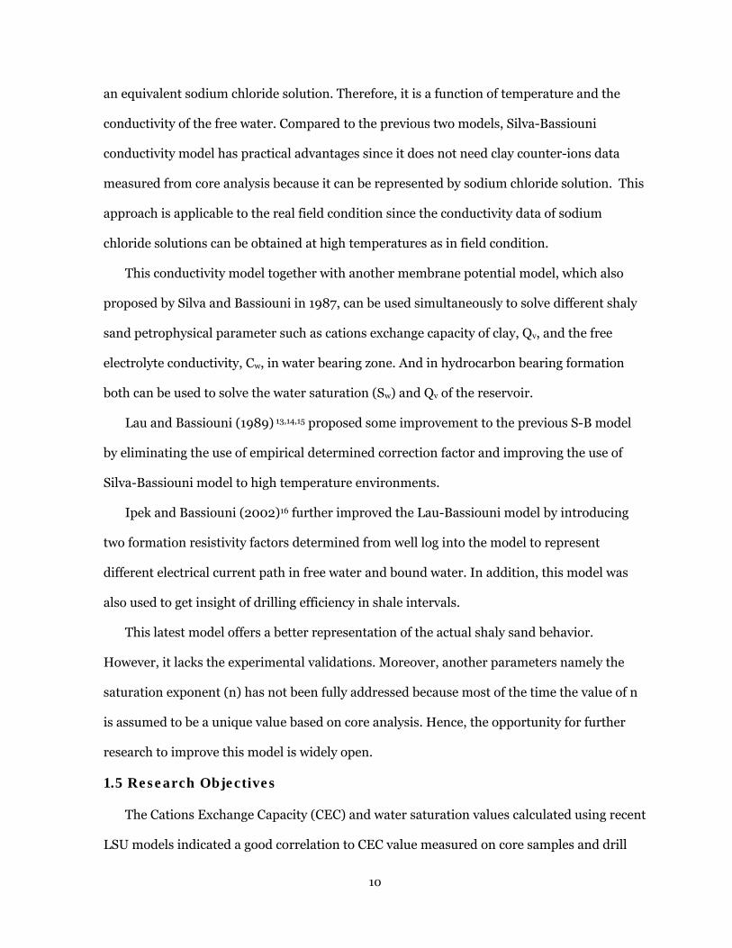
Lau and Bassiouni (1989) 13,14,15 proposed some improvement to the previous S-B model

by eliminating the use of empirical determined correction factor and improving the use of

Silva-Bassiouni model to high temperature environments.

Ipek and Bassiouni (2002)16 further improved the Lau-Bassiouni model by introducing

two formation resistivity factors determined from well log into the model to represent

different electrical current path in free water and bound water. In addition, this model was

also used to get insight of drilling efficiency in shale intervals.

This latest model offers a better representation of the actual shaly sand behavior.

However, it lacks the experimental validations. Moreover, another parameters namely the

saturation exponent (n) has not been fully addressed because most of the time the value of n

is assumed to be a unique value based on core analysis. Hence, the opportunity for further

research to improve this model is widely open.

1.5 Research Objectives

The Cations Exchange Capacity (CEC) and water saturation values calculated using recent

LSU models indicated a good correlation to CEC value measured on core samples and drill

11

cuttings and the actual production and well test data, respectively. The water saturation

calculated using these new models was found to yield more representative evaluation of

hydrocarbon potential of the zones of interest. However, the new approach using two

formations resistivity factor lacks experimental verification. Hence, the first objective is to

verify the above assumption using experimental measurement of electrical properties of three

different types of formation, namely clean sand, pure shale, and shaly sand.

There is another parameter in shaly sand analysis that is not addressed properly. This

parameter is the saturation exponent (n). Most of the time the value of saturation exponent is

assigned based on the data from clean sand core analysis. Otherwise, some correlations are

used to determine this parameter. Therefore, the second objective of this study is to

incorporate a CEC-dependent saturation exponent based on the proposed experimental

work.

Porosity estimation is a very important part of shaly sand evaluation, especially in water

saturation determination. The first objective of this research is to improve the porosity

estimation from porosity tools measurement such as density and neutron tools using a more

representative shaly sand volumetric model description. The existing volumetric model

describe the shaly sand consist of liquid-filled pore space, volume of shale and matrix.

However, this model does not address the effect of clay minerals type, clay bound water and

dry shale in the evaluation. Hence, the third objective is to modify and to improve the

existing porosity models so that a more representative evaluation of porosity in shaly sand

can be achieved.

In thin beds sand-shale sequences resistivity anisotropy can present a major problem in

quantifying the saturation of the sand layers. In a condition where the thin beds consist of

alternating shales and resistive hydrocarbon bearing sands, the conventional tool

measurement is dominated by the shale conductivity, hence, it can significantly

underestimate the hydrocarbon potential. The fourth objective is to improve the resistivity

12

anisotropy analysis using LSU models. Data from various formations known for their low

resistivity will be used.

Because of its complicated and simultaneous calculation, LSU models have a limitation in

practical application. Hence, the fifth objective of this study is to develop software based on

the recent LSU models capable of continuous depth processing of log data.

13

CHAPTER 2 SHALY SAND INTERPRETATION MODELS

Based on their basic concept, the shaly sand interpretation models can be loosely divided

into two groups:

1) Volume of Shale (Vsh): This group is widely used until today because it is practical and

applicable to logging data without core calibration of the shale related parameter.

However, due to the limitation of its concept, this method is open for misinterpretation.

2) Cations Exchange Capacity (CEC): This group is based on a scientific sounds concept but

less practical because it requires core calibration to the some log derived shale

parameters.

Although there are many models available, only several representative models that are widely

accepted will be discussed from here afterward.

2.1 Volume of Shale (Vsh) Models

The main approach of this group is solving the interpretation problem in calculating

porosity and saturation values free from the shale effect. This shale effect depends on the

amount of shale content in the formation hence the estimation of volume of shale (Vsh) is very

important. A number of methods have been developed to estimate the amount of shale (Vsh)

from different logging data such as gamma ray, SP, and porosity logs. The earliest attempts

were focused on developing a model based on distribution of clays, whether as shale in

laminated or dispersed in the pore space of the sandstone.

14

Based on petrographic examination of various cores, L.de witte (1950) 17 concluded that

the distributions of clays are more common in dispersed than laminated. Researchers later

on also recognized that laminated clays are not typical in many areas and dispersed clays

models are more representative of the shaly sand formation.

Hossin (1960) 18 developed a model based on the relationship between Vsh and total

porosity. In shaly sand, the wetted-shale, Vsh, is replacing some space of total porosity (φ). In

the other words Vsh is analogous to φ and the wetted-shale conductivity, Csh, is analogous to

the water conductivity reside in pore space, Cw. Consequently, the term φ2.Cw in Archie’s clean

sand equation become equivalent to Vsh2.Csh. In this model the quantity of X is represent by

Vsh2.Csh and can be expressed as:

sh2

shw

o C.VFC

C += [2.1]

where:

Co = conductivity of water-saturated reservoir rock, mho/m

Csh = conductivity of shale, mho/m

Vsh = volume of shale, fraction

Simandoux (1963)9 proposed a model based on the experimental work on homogeneous

mixtures of sand and montmorillonite. The quantity X in this model is represented by the

term of Vsh.Csh. Different X value compare to Hossin equation is because the montmorillonite

used in this experiment was not in fully wetted state as indicated by Hossin. This model is

given by:

shshw

o C.VFC

C += [2.2]

Poupon and Leveaux (1971)10 developed a model based on field data from Indonesia

where the reservoir rock has fresh formation water and high degree of shaliness. This model

is known as “Indonesia formula” and expressed as:

15

sh2

Vsh1

shw

o C.VFC

C −+= [2.3]

Fertl and Hammack (1971)19 proposed an empirical model based on reservoir data U.S.

gulf coast. The quantity X in this model has an interactive term represents relationship

between the electrolyte and shale components. This model is given as:

w

shshwo C324.0

C.VFC

C += [2.4]

In water saturation (Sw) term, Fertl and Hammack model has a practical aspect because it

treats the shale effect as a correction term subtracted from the clean sand term, as shown in:

⎟⎟⎠

⎞⎜⎜⎝

⎛φ

−=sh

wsh

t

ww R4.0

R.VRR.F

S [2.5a]

where:

2

81.0F

φ= [2.5b]

and:

Rw = resistivity of formation water, ohm.m

Rt = resistivity of reservoir rock, ohm.m

Rsh = resistivity of shale, ohm.m

φ = porosity of reservoir rock, fraction

It is important to note that none of the equations above represent complete coverage of

rock conductivity data over all area, linear and non-linear as shown in Figure 1.4. Equations

such as Hossin and Simandoux work well in the linear zone where as Poupon-Leveaux and

Fertl-Hammack accommodate well in the non-linear zone.

Although Vsh models are widely used because of their practicality, but to apply them in

the evaluation, there are several disadvantages need to be considered such as:

1. There is no one “universal” model available.

16

2. The Vsh parameter does not take into account the composition of constituent shale or the

type of shale.

3. The assumption of one geometric factor, F, as in clean sand is not fully supported in shaly

sand.

2.2 Cations Exchange Capacity (CEC) Models

Winsaur and McCardell (1953)20 described the phenomenon of abnormal resistivity

behavior of shaly sand. They proposed an ionic double-layer concept to describe this

phenomenon. The main difference between this model and the earlier works is the shale

conductivity is not assumed to be constant, it vary depend on the electrolyte conductivity.

Hill and Milburn (1956)21 indicated a non-linear logarithmic relationship between

formation resistivity and formation water resistivity using large amount of water-saturated

shaly sand core samples. They also demonstrated that cations exchange capacity (CEC) can

be used as an effective shaliness indicator. However, the main limitation to apply this method

is the dependency of CEC data measured from core but not from logs data. This model is

given:

( ) )R100(logbw01.0a

w

o wR100FFRR

== [2.6a]

where

Fa = apparent formation resistivity factor

F0.01 = formation resistivity factor extrapolated to a hypothetical saturating solution

of 0.01 ohms-m at 77oF

and b is function of CEC:

0055.0PVCEC

135.0b −⎟⎠

⎞⎜⎝

⎛−= [2.6b]

where:

CEC = cations exchange capacity, meq/100gram

17

PV = pore volume, fraction

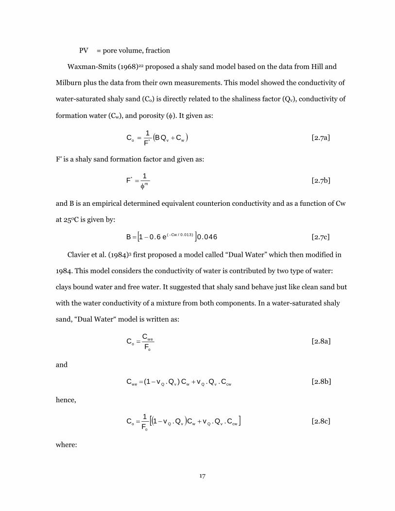
Waxman-Smits (1968)22 proposed a shaly sand model based on the data from Hill and

Milburn plus the data from their own measurements. This model showed the conductivity of

water-saturated shaly sand (Co) is directly related to the shaliness factor (Qv), conductivity of

formation water (Cw), and porosity (φ). It given as:

( )wv*o CQBF1

C += [2.7a]

F* is a shaly sand formation factor and given as:

m

* 1F

φ= [2.7b]

and B is an empirical determined equivalent counterion conductivity and as a function of Cw

at 250C is given by:

[ ] 046.0e6.01B )013.0/Cw(−−= [2.7c]

Clavier et al. (1984)3 first proposed a model called “Dual Water” which then modified in

1984. This model considers the conductivity of water is contributed by two type of water:

clays bound water and free water. It suggested that shaly sand behave just like clean sand but

with the water conductivity of a mixture from both components. In a water-saturated shaly

sand, “Dual Water“ model is written as:

o

weo F

CC = [2.8a]

and

cwvQwvQwe C.Q.vC)Q.v1(C +−= [2.8b]

hence,

( )[ ]cwvQwvQo

o C.Q.vCQ.v1F1

C +−= [2.8c]

where:

18

Cwe = equivalent conductivity of mixture water

Fo = formation resistivity factor associated with total porosity

vQ = amount of clays associated with 1 unit (meq) of clays counterions

Qv = cations exchange capacity

Ccw = conductivity of clays bound water

Best et al. (1978)23 introduced a shaly sand model, which was intended to be used wellsite

computer interpretation process called “CYBERLOOK”. This model was inspired by the “Dual

Water” concept. The CYBERLOOK model is given as:

[ ]wFwBwBwB2

to C)S1(CSC −+φ= [2.9a]

and the total porosity (φt) and the bound water saturation (SwB) are defined as:

wFwBt φ+φ=φ [2.9b]

t

wBwBS

φφ

= [2.9c]

where:

φwB = porosity occupied by bound water

φwF = porosity occupied by free water

The conductivity of the bound water (CwB) and free water (CwF), are estimated in a pure shale

and a clean water-bearing formation, respectively:

*

sh

2sht

wBC

)(C

φ= [2.9d]

*

o

2sst

wFC

)(C

φ= [2.9e]

where:

(φt)sh = total porosity in pure shale, fraction

(φt)ss = total porosity in clean sand, fraction

19

Csh* = conductivity of pure shale, mho/m

Co* = conductivity of clean sand, mho/m

Juhasz (1981)24 proposed a more practical version of Waxman-Smits model because Qv

can be calculated from logs data rather than core. The term Qv in Waxman-Smits is replaced

by Qvn, normalized Qv. This Qvn term is expressed as:

t

shtsh

vsh

vvn

)(VQQ

Qφφ

== [2.10]

The cations exchange capacity (CEC) interpretation models led to a better understanding

of clay effect on the electric conductivity of rocks that take into account the both clay volume

and clay type. However, there are still many limitation of using these models mainly due to

the need of CEC measured from rock samples in laboratory environments. Although there are

some methods to calculate the CEC directly from well-log data, they still need CEC

measurement from the rock to calibrate the result.

2.3 Discussion

The ability to estimate CEC directly from well-log and to eliminate the need for rock

measurement improves the overall process in shaly sand interpretation. This ability can

reduce or even eliminate the need to do the expensive coring job for obtaining core samples.

Moreover, it can increase the estimation confident because all the input data is acquired from

in-situ downhole condition.

Recognizing this matter, researchers at Louisiana State University have started since 1985

the development of the shaly sand interpretation from a more theoretical approach. There are

three models have been developed during this time namely Silva-Bassiouni (1985), Lau-

Bassiouni (1989), and Ipek-Bassiouni (2002). The LSU model is based on the Waxman and

Smits concept of supplementing the water conductivity with clay counterions conductivity

and the Dual Water theory, which considers two waters each occupying a specific volume of

the total pore space. However, LSU models are different from those concepts because it treats

20

the counterion conductivity as a hypothetical sodium chloride solution. A more detail

discussion of the history of LSU model is described in the following chapter.

21

CHAPTER 3 DEVELOPMENT OF LSU SHALY SAND MODEL

Over the years researchers at Louisiana State University have proposed numbers of shaly

sand models based on Waxman-Smits (1968)11 concept, which relates the water conductivity

with clays counterions, and the Dual Water theory (1984)3, which relates two water

conductivity terms in shaly sand, clay bound and free water, that occupying a specific volume

of the total pore space. However, in the LSU models the counterion conductivity is

represented by a hypothetical sodium chloride solution.

3.1 Silva-Bassiouni (S-B)

Silva-Bassiouni proposed a new theoretical derived model for shaly sand. The model

consists of two types: conductivity model and membrane potential model. Detailed

description is given hereafter.

3.1.1 Conductivity Model

Silva-Bassiouni addressed the conductivity anomaly in shaly sand by treating the excess

conductivity generated by the transport of electric current by counterions associated with

clay minerals, known as double layer, as that of an equivalent sodium chloride solution.

Moreover, the shaly sand conductive behavior is assumed to be similar to that of clean sand

of the same porosity3. The effective conductivity, Cwe or equivalent

counterions conductivity, Cwe, is the sum of the conductivity of diffused double layer and the

conductivity of free water and given as:

wfdlclfdlwe C)v1(C.vC −+= [3.1]

22

The fractional volume of double layer (vfdl) and the conductivity contribution of the exchange

cations associated with clays (Ccl) are expressed as:

vw

fdl Q22.0C084.0

v ⎟⎟⎠

⎞⎜⎜⎝

⎛+= [3.2]

+= eqeqcl n.cC [3.3]

where Qv is the cations exchange capacity per total pore volume. The equivalent

concentration of clay counterions (neq) are estimated based on the equivalent sodium

chloride solution as25:

( )2dl

eq

188.0f

571.3n

−=+ [3.4]

where, at temperature of 25oC, fdl defined as the double layer expansion factor is given as12:

2/12o

2hdl )n.B.X(f −= [3.5]

where, Xh is 6.18 Å and n is the free water concentration. Bo is a function of temperature

given by25:

274o T.10x935.8T.10x5108.13248.0B −− ++= [3.6]

In this model, at temperature of 25oC, neq+ can also be expressed in term of Qv as:

fdl

veq v

Qn =+ [3.7]

The equivalent conductivity of clay counterions (ceq) is also defined as the equivalent of

sodium chloride solution as:

)]ne(F.f[

'cc

g

eqeq = [3.8]

where ceq’ is the equivalent conductivity of the equivalent sodium chloride solution. At

temperature of 25oC, ceq’ is given by:

eq

eqeq

n3164.11

n6725.7645.12'c

+

+= [3.9]

23

The term fg and F(ne)are empirical determined correction factors. At temperature of 25oC,

these terms are expressed as:

cn/1dlg ff = [3.10]

where,

2dldlc f14426.0f1796.16696.0n −+= [3.11]

and,

2eq

2eq

2 )5.0n(10x761.1)5.0n(10x83.31)ne(F −+−+= −− ; neq>0.5 mol/l [3.12a]

1)ne(F = ; neq≤0.5 mol/l [3.12b]

Based on this S-B model, in a fully brine saturated shaly sand, the formation conductivity is

given as:

e

wfdlfdleqeq

e

weo F

]C)v1(v.n.c[

FC

C−+

==+

[3.13]

where Fe is the formation resistivity factor expressed as:

cmeF φ= [3.14]

and, mc is the cementation exponent.

3.1.2 Membrane Potential Model

Silva-Bassiouni proposed a modified membrane potential (Em) expression introduced by

Thomas (1976)26. In the modification a correction factor (τ) was introduced to address a

deviation of membrane potential in saturated salt solution. Hence, the membrane potential

model is given by:

∫ ±γτ−

= +1m

2mm )mln(dTna

FTR2

E [3.15]

where:

R = universal gas constant

F = Faraday constant

24

T = absolute temperature (oK)

Tna+ = sodium transport number

m = molal concentration (mol/kg)

γ± = mean activity coefficient

and

w

wnwv C

)CC(Q28.01

−−=τ ; Cw > Cwn [3.16a]

1=τ ; Cw ≤ Cwn [3.16b]

Cwn = 16.61 mho/m at 25oC

The sodium transport number (Tna+) are used because S-B model assumed the two

electrolytes exist in shaly sand (clay bound water and free water) which act parallel to each

other can be treated as sodium chloride solution. Therefore, the Tna+ is expressed as:

wfdlveq

wfdlh

veq

C)v1(Q.c

C)v1(tnaQ.cTna

−+

−+=+ [3.17]

where tnah is the Hittorf transport number defined as the motion of ions relative to that of

water and derived by Stokes (1955) as27:

n.726.15545.126

n.402.551.50tnah

+

+= [3.18]

where n is the molar concentration of the free water.

At 25oC, the mean activity coefficient (γ±) of sodium chloride solution is defined as:

)m.027.01log()alog(75.1n.3065.11

n.5115.0)(log A −−−

+

−=±γ [3.19]

where:

n = molar concentration (mol/l)

m = molal concentration (mol/kg)

and,

25

aA = 0.99948 – 0.03959.m – 0.0015075 m2 [3.20]

The calculated values using this model showed a remarkable agreement with published

experimentally determined values. However, because this model uses some empirical

correction factors determined at 25oC, there is some limitation in applying this model to the

field condition.

3.2 Lau-Bassiouni (L-B)

Lau-Bassiouni proposed a modification of S-B model by eliminating the use of empirically

derived correction factor. This modification extends the application of S-B model

temperature higher than 25oC or closer to the actual field condition.

3.2.1 Conductivity Model

Lau-Bassiouni introduced a modified fractional volume of double layer (vfdl) by taking

into account the effect of temperature as:

v2

o2

h

afdl Q

)n.B.X(

)298/T(25

Tln0344.028.0v⎥⎥

⎦

⎤

⎢⎢

⎣

⎡

⎥⎦⎤

⎢⎣⎡

⎟⎠⎞⎜

⎝⎛−= [3.21]

where:

T = temperature, oC

Ta = absolute temperature, oK

Xh = 6.18 Å

and, the free water concentration (n) can be estimated using the expression below28:

wwaa C00467.0)Cln(1851.1T0229.0)Tln(58.131.68)nln( +++−= [3.22]

Lau-Bassiouni defined the equivalent concentration of clay counterions (neq) as a function of

temperature as:

⎟⎟⎠

⎞⎜⎜⎝

⎛⎟⎟⎠

⎞⎜⎜⎝

⎛=⎟⎟

⎠

⎞⎜⎜⎝

⎛= +

298T

vQ

298T

nn a

fdl

vaeqeq [3.23]

26

To estimate the counterions conductivity (ceq), Lau-Bassiouni eliminated the use of the

correction factors and instead using published experimental data28. The expression for ceq is

given by:

)Tln(85.11T0216.0)nln(07871.0n1026.084.58)cln( aaeqeqeq +−−−−= [3.24]

In a fully brine saturated shaly sand, the formation conductivity is given by:

e

wfdlfdleqeqo F

]C)v1(v.n.c[C

−+= [3.25]

In formations saturated with hydrocarbon, Qv should be corrected for the water saturation

effect as given by:

w

vv S

Q'Q = [3.26]

3.2.2 Spontaneous Potential Model

Lau-Bassiouni extended the use of S-B membrane potential model to a theoretical model

based on the response of spontaneous potential (SP) log. They postulated, considering the

electrokinetic effects are neglected, the deflection of SP curve in front of permeable

formations is generated from the difference of the electrochemical potential of shales (Emsh)

and adjacent sands (Emss)29. Hence, the SP model can be expressed as:

sssh EmEmSP −= [3.27]

In the general term of transport number, equation [3.8] can be re-written as:

( ) )mln(dTnaTnaF

TR2SP

1m

2m

sssh ±γ−−= ∫ [3.28]

In case of pure shale, it is not possible to compute Cw from wireline data, therefore Tnash

can not be determined theoretically. To simplify this matter, most of the time it is assumed

that shale behave as a perfect shale or in the other words Tnash = 1. However, this is not

always correct, because the free water always exist in the pore space. Hence, an empirical

parameter, namely the membrane efficiency (meff) was introduced to represent Tnash.

27

Equation [3.28] can be further extended using the general term of sodium transport number

(tna+) to become:

)mln(dC)v1(v.n.c

C)v1(tnav.n.c

FTR2

)mln(dmF

TR2SP

1m

2m wfdlfdleqeq

wfdlfdleqeq1m

2meff ±γ

−+

−++±γ−= ∫∫

+

[3.29]

The sodium chloride transport number, tna+, is estimated from:

wh ttnatna +=+ [3.30]

where tnah and tw are the Hittorf transport number and water transport number, respectively.

The tnah can be estimated using the following expression30:

m.T.10x41764.1

)Tln(264709.0)mln(10x803769.150893.2)tnaln(

a5

a2h

−

−

−

+−−= [3.31]

where:

Ta = absolute temperature, oK

m = molality, mol/kg

The water transport number, tw, is expressed as function of molality and Qv as13:

vw Q]1244.0)mln(.1961.0[043.0m.053.0t ++−= ; m≤1.0 [3.32a]

v1.1

w Q04.004377.0m.036.0t +−= ; m>1.0 [3.32b]

The mean activity coefficient (γ±) is affected by temperature and expressed as31:

298298298 J.Z5.0L.Y5.0)log()log( −+±γ=±γ [3.33]

where (γ±)298 is the activity coefficient at 25oC defined as:

)m.027.01log()alog(75.1n3065.11

n5115.0)log( A

298 −−−+

−=±γ [3.34]

and,

22A m.0015.0m.10x0959.399948.0a −−= − [3.35]

)T(3026.2)15.298(3147.8

T15.298Y

a

a−= [3.36]

28

⎟⎟⎠

⎞⎜⎜⎝

⎛+=

15.298T

log3147.81

Y15.298Z a [3.37]

3298 m5.986m8.3182

m1

m6.2878L +−

+= [3.38]

3298 m36.20m72

m1

m5.43J −+

+= [3.39]

This new model was tested over a wide range of temperature, water saturations and water

salinities. The calculated values display a remarkable agreement with experimentally

determined values. The most application advantage for this model is the ability to combine

both conductivity and SP model to solve simultaneously for Qv, Sw, and Cw using conventional

well log measurements. However, there is still parameter in the models, which are not fully

addressed, namely the formation resistivity factor. This model still use one expression of

formation resistivity factor two different ion paths clay bound water and free water.

3.3 Ipek-Bassiouni (I-B)

Ipek-Bassiouni further improves of L-B model by better describing the formation

resistivity factor. This model incorporate two different formation factors to represent clay

bound water and free water. The premise of this approach is that current paths around the

clay bound water are different from the current paths in the free water.

3.3.1 Conductivity Model

Ipek-Bassiouni proposed two formations resistivity factors incorporated into the new

conductivity model for shaly sand. Hence in brine saturated shaly sand, the parallel

conductance of free water and clay bound water is expressed as:

bw

cl

fw

wo F

CFC

C += [3.40]

where:

Cw = formation water conductivity, mho/m

Ccl = clay conductivity, mho/m

29

and, Ffw and Fbw are the formation resistivity factors for free water and clay bound water,

respectively. Both are defined as:

fm

e

fw1

Fφ

= [3.41a]

cm

bw

bw1

Fφ

= [3.41b]

where:

mf = cementation exponent of free water

mc = cementation exponent of bound water

and, φe and φbw are the effective porosity and bound water porosity, respectively. Both

parameters are given by32:

)v1( fdlte −φ=φ [3.42]

fdltetbw v.φ=φ−φ=φ [3.43]

where φt and vfdl are the total porosity and fractional volume of double layer, respectively.

By substituting equation [3.42], equations [3.43], equation [3.41a], and equation [3.41b] into

equation [3.40], a new conductivity model can be derived. Assuming the counterions

conductivity can be represented by that of equivalent sodium chloride solution, in brine

saturated shaly sand, this model is defined by:

].v.n.c.)v1(C[C ccff mmfdleqeq

mmfdlwo φ+φ−= [3.44]

The cementation exponent of free water (mf) and clay bound water (mc) can be

determined using log data from a particular interval in clean sand and pure shale of the same

geological unit, respectively. In clean sand, constructing a log-log plot between Co vs. φ will

result in a linear trend where the slope is representing mf. With the same approach in pure

shale, the linear relationship slope log-log plot between Csh vs. φ is equal to mc.

30

3.3.2 Spontaneous Potential Model

Based on the different formation resistivity factor used in the model, the expression of

sodium transport number (Tna+) can be modified to become:

w

mfdl

mfdleqeq

wm

fdlm

fdleqeq

C)v1(v.n.c

C)v1(tnav.n.cTna

fc

fc

−+

−+=

++ [3.45]

By substituting equation [3.45] into the Lau-Bassiouni SP model, Ipek-Bassiouni has further

improved the SP model to better address the rock and fluid properties in shaly sand. This

new model can be expressed as:

)mln(dC)v1(v.n.c

C)v1(tnav.n.c

FTR2

)mln(dmF

TR2SP

1m

2m wm

fdlm

fdleqeq

wm

fdlm

fdleqeq1m

2meff

fc

fc

±γ−+

−++±γ−= ∫∫

+

[3.46]

3.4 Discussion

This most recent LSU model proposed by Ipek-Bassiouni eliminated the assumption that

similar resistivity factor is applied to both clay bound water and free water. In the other

words this model considered the different current path should be addressed by different

formation factors. Although the calculation values yield a representative result than the

previous model, this model lacks experimental validation.

Therefore, further laboratory work in proposed to validate the most recent LSU model.

This laboratory work will use different type of formation, actual and artificial. Moreover, this

experimental work will try to incorporate a Qv-dependent saturation exponent (n*) into the

LSU model to get a complete representation of rock and fluid properties in shaly sand.

31

CHAPTER 4 DUAL FORMATION RESISTIVITY FACTOR

The latest LSU model (Ipek-Bassiouni) proposed the use of two formation resistivity

factors determined directly from log data to represent resistivity effect of free water and

bound water to the overall resistivity of shaly rocks. This model indicated a better estimation

of water saturation in shaly sand reservoirs. In addition, the value of cations exchange

capacity (Qv) insitu reservoir condition can also be estimated within reasonable accuracy.

However, the idea of using two formation resistivity factors in LSU model lacks experimental

validation. To further improve this model, sets of experimental work had been made using

actual reservoir rocks from South Louisiana field characterized by high degree of shaliness.

The experimental work can provide important information concerning the rock and fluid

behavior such as:

1). The behavior of ion path in free water and clay bound water that is represented by the

degree of the rock tortuosity. The tortuosity degree has a direct relationship with the rock

cementation exponent because it is a function of the shape and distribution of pores.

Therefore cementation exponent (m) of a formation often used to indicate its tortuosity8.

Cementation exponent in free water (mf) and clay bound water (mc) can be measured

from clean sand and pure shale, respectively;

2). By determining mf and mc there is a chance to improve the definition of the relationship

between formation resistivity factor of free water (Ff) and clay bound water (Fc) because

formation resistivity factor (F) is a function of cementation exponent (m).

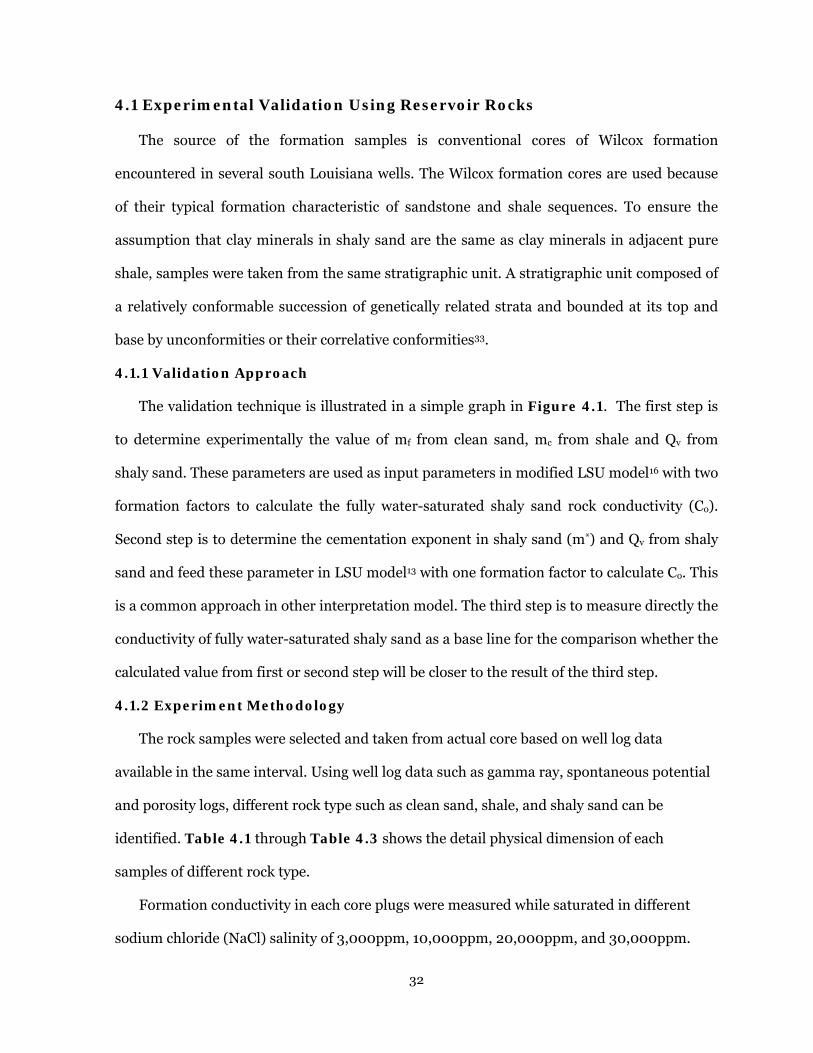
32

4.1 Experimental Validation Using Reservoir Rocks

The source of the formation samples is conventional cores of Wilcox formation

encountered in several south Louisiana wells. The Wilcox formation cores are used because

of their typical formation characteristic of sandstone and shale sequences. To ensure the

assumption that clay minerals in shaly sand are the same as clay minerals in adjacent pure

shale, samples were taken from the same stratigraphic unit. A stratigraphic unit composed of

a relatively conformable succession of genetically related strata and bounded at its top and

base by unconformities or their correlative conformities33.

4.1.1 Validation Approach

The validation technique is illustrated in a simple graph in Figure 4.1. The first step is

to determine experimentally the value of mf from clean sand, mc from shale and Qv from

shaly sand. These parameters are used as input parameters in modified LSU model16 with two

formation factors to calculate the fully water-saturated shaly sand rock conductivity (Co).

Second step is to determine the cementation exponent in shaly sand (m*) and Qv from shaly

sand and feed these parameter in LSU model13 with one formation factor to calculate Co. This

is a common approach in other interpretation model. The third step is to measure directly the

conductivity of fully water-saturated shaly sand as a base line for the comparison whether the

calculated value from first or second step will be closer to the result of the third step.

4.1.2 Experiment Methodology

The rock samples were selected and taken from actual core based on well log data

available in the same interval. Using well log data such as gamma ray, spontaneous potential

and porosity logs, different rock type such as clean sand, shale, and shaly sand can be

identified. Table 4.1 through Table 4.3 shows the detail physical dimension of each

samples of different rock type.

Formation conductivity in each core plugs were measured while saturated in different

sodium chloride (NaCl) salinity of 3,000ppm, 10,000ppm, 20,000ppm, and 30,000ppm.

33

Figure 4.1: The validation of LSU model using two formation factors to calculate shaly sand electrical properties.

These low salinity concentrations were chosen mainly because the complexity of shaly sand

evaluation occurs at low salinity values. For each particular salinity, core plugs were prepared

in several steps such as cleaning, drying, evacuating and saturating. After saturating in

sodium chloride solution (NaCl) for 24 hours, conductive paint was then applied on top and

bottom flat surfaces of all core plugs to get a more homogeneous measurement.

Measurements were taken for different descending water saturation value starting from

100%. Saturation less than 100% is achieved by exposing the core to the air allowing water to

evaporate. These saturations are determined by the weigh of core plugs in every sequence of

measurement. Then core conductivity in each saturation step is measured using conductivity

apparatus.

4.1.3 Experiment Apparatus

An impedance analyzer Hewlett-Packard 4279A LCZ meter is used to measure the

electrical resistivity of the core samples under varying degree of brine saturation. The LCZ

meter is capable of measuring inductance, capacitance, dissipation, quality factor, impedance

magnitude, and phase angle in equivalent parallel and series circuits34.

Clean Sand

mf

Shale

mc

Shaly Sand

Qv

Modified LSU Model

Co

Shaly Sand

Qvm*

LSU Model

Co

Shaly Sand

Experiment

Co

Clean Sand

mf

Clean SandClean SandClean Sand

mf

Shale

mc

ShaleShaleShale

mc

Shaly SandShaly SandShaly Sand

Qv

Modified LSU Model

Co

Shaly Sand

Qvm*

LSU Model

Co

Shaly Sand

Qvm*

Shaly SandShaly Sand

Qvm*

LSU Model

Co

Shaly Sand

Experiment

Co

Shaly Sand

Experiment

Shaly Sand

Experiment

Co

34

Table 4.1: Geometric properties of clean sand rock samples used in the experimental measurement

Table 4.2: Geometric properties of shale rock samples used in the experimental measurement

Diameter Length Dry Weight Porosity[mm] [mm] [gram] [v/v]

CS-1L Clean Sand 25.53 43.84 46.71 0.1513CS-2L Clean Sand 25.55 38.85 41.77 0.1523CS-3L Clean Sand 25.52 43.87 47.20 0.1538CS-4L Clean Sand 25.52 44.98 47.97 0.1527CS-5L Clean Sand 25.54 43.87 47.35 0.1448CS-7L Clean Sand 25.53 38.87 41.89 0.1539CS-8L Clean Sand 25.55 38.29 41.07 0.1458CS-9L Clean Sand 25.55 42.18 44.72 0.1497CS-1U Clean Sand 25.51 42.75 46.70 0.1286CS-2U Clean Sand 25.51 44.98 49.57 0.1279CS-3U Clean Sand 25.52 45.56 50.50 0.1288CS-5U Clean Sand 25.52 45.55 50.60 0.1292CS-7U Clean Sand 25.51 43.86 48.46 0.1234CS-8U Clean Sand 25.51 37.77 43.67 0.1081CS-9U Clean Sand 25.53 41.64 46.78 0.1183

Core Number Description

Diameter Length Dry Weight Porosity[mm] [mm] [gram] [v/v]

SH-1 Shale 25.54 18.87 22.17 0.0864SH-2 Shale 25.53 19.95 23.27 0.0852SH-3 Shale 25.55 18.87 22.51 0.0872SH-4 Shale 25.54 17.75 21.25 0.0813SH-5 Shale 25.54 18.85 22.41 0.0747SH-6 Shale 25.53 16.65 19.69 0.0755SH-7 Shale 25.54 17.77 21.78 0.0745SH-8 Shale 25.52 18.32 22.59 0.0724SH-9 Shale 25.53 17.76 21.68 0.0842SH-10 Shale 25.53 18.28 21.83 0.0734SH-11 Shale 25.53 18.29 22.18 0.0715SH-12 Shale 25.53 19.95 24.26 0.0775SH-13 Shale 25.54 19.86 23.01 0.0735

Core Number Description

35

Table 4.3: Geometric properties of shaly sand rock samples used in the experimental measurement

These measurements cover a frequency range from 100 Hz to 20 kHz with steps of 100 Hz.

The HP 4297A model is controlled by a personal computer via a HP-IB card and Agilent VEE

Pro software. The card and software allow the digitalization of measured data for further

analysis and interpretation. Figure 4.2 shows the conductivity apparatus used for electrical

properties measurement.

The impedance analyzer is equipped with four coaxial BNC connectors and with an HP

16047A test feature. This feature combines the high and low voltage and current terminals

and permits two terminal measurements of the electrical properties of the samples. The two-

terminal measurement method is a simple procedure to apply but has some drawbacks

compared to other methods. One of the main drawbacks is the electrode polarization

problem. The rock-electrode interface feels the movement of ions and cations on the rock

sample and the movement of electrons on the electronic circuit. At this interface blocking

electrodes is commonly found (i.e., electrodes that do not experience oxidation-reduction)

and causing an accumulation of ions at the interface that generate the electrode polarization.

Based on modeling study, electrode polarization has a negligible effect on high-frequency

measurement35. The use of silver paint electrodes can also reduce the effect of electrode

Diameter Length Dry Weight Porosity[mm] [mm] [gram] [v/v]

SHY-1 Shaly Sand 25.53 38.85 47.19 0.0726SHY-2 Shaly Sand 25.53 37.76 44.06 0.0990SHY-3 Shaly Sand 25.52 39.97 46.43 0.0881SHY-4 Shaly Sand 25.53 36.66 45.49 0.0908SHY-5 Shaly Sand 25.52 39.99 48.41 0.0841SHY-6 Shaly Sand 25.53 34.98 41.10 0.1059SHY-7 Shaly Sand 25.52 37.67 44.98 0.0758SHY-10 Shaly Sand 25.51 38.84 46.61 0.0749SHY-11 Shaly Sand 25.53 40.54 47.86 0.0888SHY-12 Shaly Sand 25.51 38.34 46.00 0.0759SHY-13 Shaly Sand 25.52 40.55 46.71 0.0902

Core Number Description

36

Figure 4.2: The setup of conductivity apparatus for electrical properties measurement of three type of rock: clean sand, shaly sand, and shale.

polarization because it keeps the gap between sample and the electronic circuit constant

throughout the measurement series36. Hence, to ensure acquiring consistent and reliable data

all the measurement were conducted in high-frequency and silver paint was applied on top

and bottom of all samples.

4.2 Cementation Exponent Determination

The latest LSU model incorporates two cementation exponents: free water (mf) and clay

bound water (mc). The mf and mc are estimated directly from log data in adjacent clean sands

and pure shale, respectively. To validate this assumption, both parameters were determined

experimentally. Series of laboratory measurement of formation electrical properties will be

conducted. Based on the experimental result, mf and mc can be determined from the

relationship between porosity and formation resistivity factor. According to Archie’s general

relationship, the relationship between porosity and formation resistivity factor for free water

(Ff) and bound water (Fc) is given, respectively, as:

mf

sd

f

1F

φ= [4.1]

mc

sh

c

1F

φ= [4.2]

Impedance Analyzer

Personal Computer

High Current and Voltage Terminals

Low Current and Voltage Terminals

Core Sample

Impedance Analyzer

Personal Computer

High Current and Voltage Terminals

Low Current and Voltage Terminals

Core Sample

Impedance Analyzer

Personal Computer

High Current and Voltage Terminals

Low Current and Voltage Terminals

Core Sample

37

Since formation resistivity factor is also defined as the ratio of resistivity of rock fully

saturated with water (Ro or Rsh) to the resistivity of water (Rw), equation [4.1] and [4.2] can

be modified to:

sdfw

of log.m

RR

logFlog φ−=⎟⎟⎠

⎞⎜⎜⎝

⎛= [4.3]

shcw

shc log.m

RR

logFlog φ−=⎟⎟⎠

⎞⎜⎜⎝

⎛= [4.4]

The parameters Ro, Rsh, Rw, φsd and φsh are determined from experimental measurement;

hence, mf and mc can be estimated.

• Clean Sand. The cementation exponent of free water (mf) in shaly sand is assumed to be

similar to that of the adjacent clean sand hence by measuring the electrical properties in

clean sand, the relationship between the formation resistivity factor and porosity can be

established. The slope of this relationship represents the cementation exponent of free water

(mf). Figure 4.3 through Figure 4.6 show the estimation of mf based on resistivity

measurement of clean sand rocks in different brine concentrations, namely 3,000ppm,

10,000ppm, 20,000ppm and 30,000ppm.

The cementation exponent of free water (mf) determined from clean sand indicates a

variation in cementation exponent value in different salinity (Figure 4.7). This is interesting

because in a clean sand sample brine is the only conducting medium, hence the cementation

exponent (mf) that represents the ions movement through a tortuous path should not vary

with salinity.

Possible explanation for this behavior is that the samples are not fully clean but contain

some degree of shaliness. Some clay particles in the rock samples will exhibit a net negative

charge that is compensated for by the accumulation of cations near the particle surface

(Figure 4.8). Hence in clay-liquid system, a double layer of electrical charge exists. The

double-layer thickness or the bound water thickness decreases as the brine concentration

38

Figure 4.3: Relationship between formation resistivity factor and porosity of clean sand in 3,000 ppm brine salinity. The slope represents its cementation exponent value (mf).

Figure 4.4: Relationship between formation resistivity factor and porosity of clean sand in 10,000 ppm brine salinity. The slope represents its cementation exponent value (mf).

3,000 ppm NaCl

1

10

100

0.1 1

Porosity (v/v)

Form

atio

n Fa

ctor

(R

o/R

w)

CS-1UCS-2UCS-3UCS-5UCS-7UCS-8UCS-9UCS-1LCS-2LCS-3LCS-4LCS-5LCS-6LCS-7LCS-8LCS-9L

mf = 1.301

3,000 ppm NaCl

1

10

100

0.1 1

Porosity (v/v)

Form

atio

n Fa

ctor

(R

o/R

w)

CS-1UCS-2UCS-3UCS-5UCS-7UCS-8UCS-9UCS-1LCS-2LCS-3LCS-4LCS-5LCS-6LCS-7LCS-8LCS-9L

mf = 1.301

10,000 ppm NaCl

1

10

100

0.1 1

Porosity (v/v)

Form

atio

n Fa

ctor

(R

o/R

w)

CS-1UCS-2UCS-3UCS-5UCS-7UCS-8UCS-9UCS-1LCS-2LCS-3LCS-4LCS-5LCS-6LCS-7LCS-8LCS-9L

mf = 1.568

10,000 ppm NaCl

1

10

100

0.1 1

Porosity (v/v)

Form

atio

n Fa

ctor

(R

o/R

w)

CS-1UCS-2UCS-3UCS-5UCS-7UCS-8UCS-9UCS-1LCS-2LCS-3LCS-4LCS-5LCS-6LCS-7LCS-8LCS-9L

mf = 1.568

39

Figure 4.5: Relationship between formation resistivity factor and porosity of clean sand in 20,000 ppm brine salinity. The slope represents its cementation exponent value (mf).

Figure 4.6: Relationship between formation resistivity factor and porosity of clean sand in 30,000 ppm brine salinity. The slope represents its cementation exponent value (mf).

20,000 ppm NaCl

1

10

100

0.1 1

Porosity (v/v)

Form

atio

n Fa

ctor

(R

o/R

w)

CS-1UCS-2UCS-3UCS-5UCS-7UCS-8UCS-9UCS-1LCS-2LCS-3LCS-4LCS-5LCS-6LCS-7LCS-8LCS-9L

mf = 1. 591

20,000 ppm NaCl

1

10

100

0.1 1

Porosity (v/v)

Form

atio

n Fa

ctor

(R

o/R

w)

CS-1UCS-2UCS-3UCS-5UCS-7UCS-8UCS-9UCS-1LCS-2LCS-3LCS-4LCS-5LCS-6LCS-7LCS-8LCS-9L

mf = 1. 591

30,000 ppm NaCl

1

10

100

0.1 1

Porosity (v/v)

Form

atio

n Fa

ctor

(R

o/R

w)

CS-1UCS-2UCS-3UCS-5UCS-7UCS-8UCS-9UCS-1LCS-2LCS-3LCS-4LCS-5LCS-6LCS-7LCS-8LCS-9L

mf = 1.763

30,000 ppm NaCl

1

10

100

0.1 1

Porosity (v/v)

Form

atio

n Fa

ctor

(R

o/R

w)

CS-1UCS-2UCS-3UCS-5UCS-7UCS-8UCS-9UCS-1LCS-2LCS-3LCS-4LCS-5LCS-6LCS-7LCS-8LCS-9L

mf = 1.763

40

Figure 4.7: The relationship between cementation exponent in clean sand (mf) and brine salinity where mf tend to increase with the increasing of brine salinity.

increases3. In low brine concentration the ions movement will follow a less tortuous path

because the bound water is thicker than in high brine concentration. Thicker bound water

will cover the area of high tortuosity in micro pore space between clay particles.

To support this explanation, laboratory measurement of CEC in the so called “clean sand”

samples were conducted and the result indicated indeed some degree of shaliness exists. This

shaliness is represented by the value of Qv of 0.5 meq/cc to 0.8 meq/cc (Table 4.4).

Figure 4.9 showed the relationship between porosity and cations exchange capacity (Qv)

measured in the clean sand. The increasing of clay content as shown by increasing of Qv value

caused a significant reduction in effective porosity value. This is another indication that the

presumably clean sand samples were in fact contain some degree of shaliness.

• Shale. The resistivity measurement in shale follows the same principle as clean sand.

However, shale has a lower effective porosity and permeability compared to clean sand.

Hence, the brine saturation process in shale using only vacuum pump might not result in

1.0

1.1

1.2

1.3

1.4

1.5

1.6

1.7

1.8

1.9

2.0

0 10,000 20,000 30,000 40,000

Brine Salinity (ppm)

Cem

enta

tion E

xp.

(mf)

41

Figure 4.8: Schematic of OHP (parallel to clay surface). The distance, XH, is determined by the amount of absorbed on clay surface and hydration water around each cation.

Table 4.4: CEC measurement result of several “clean” sand samples

Porosity Qv

[v/v] [meq/cc]

CS-3U 0.123 0.677CS-4L 0.155 0.512CS-5L 0.153 0.574CS-5U 0.123 0.745CS-7L 0.157 0.564CS-7U 0.119 0.799

Core No.

42

Figure 4.9: Increasing of clay content in “clean” sand samples is reducing the effective porosity of the formation

shale fully saturated by brine. To evaluate whether saturation process using vacuum pump is

adequate or not, another method with a higher saturating force using centrifuge pump was

used. Both centrifuge and vacuum pump indicated a similar result of saturation degree in

shale samples saturated 3,000 ppm brine as shown in Table 4.5. A good correlation

between wet weight of shale samples measured from vacuum pump and centrifuge can be

observed in Figure 4.10. For the sake of practicality, the vacuum pump was then used to

saturate all the shale samples.

Figure 4.11 through Figure 4.14 shows the estimation of the cementation exponent of

clay bound water (mc) based on resistivity measurement of shale rocks in different brine

concentrations, namely 3,000ppm, 10,000ppm, 20,000ppm and 30,000ppm. The low and

narrow range of measured value of shale porosity is affected by the natural behavior of shale

itself. Because the porosity in shale is determined from replacing the air-filled pore space

0.0

0.1

0.2

0.3

0.4

0.5

0.6

0.7

0.8

0.9

1.0

0.00 0.05 0.10 0.15 0.20 0.25 0.30

Effective Porosity [v/v]

Qv [

meq/c

c]

43

with brine, hence the measured porosity is the effective porosity. Shale has been known to

have low effective porosity.

Table 4.5: Result from saturating shale with brine using vacuum pump and centrifuge

Figure 4.10: Comparison of shale wet weight measured by vacuum pump and centrifuge in 3,000 ppm brine salinity.

All graphs indicate two groups of data, group A and group B. However, only group A

indicates a clear trend between formation resistivity factor and porosity, hence, it will be used

for further cementation exponent analysis. By constructing a linear trend to porosity of 100%,

the cementation exponent of bound water (mc) can be determined.

Dry Weight Wet Weight Dry Weight Wet Weight[gram] [gram] [gram] [gram]

SH-1 22.17 22.25 22.17 22.26SH-3 22.51 22.58 22.51 22.59SH-5 22.41 22.46 22.41 22.46SH-7 21.78 21.85 21.78 21.85SH-8 22.59 22.66 22.59 22.66

Vacuum Pump CentrifugeCore Number

21

21.5

22

22.5

23

21 21.5 22 22.5 23

W et W eight [gr]-Vacuum Pump

Wet

Weig

ht

[gr]

-Cen

trifu

g

21

21.5

22

22.5

23

21 21.5 22 22.5 23

W et W eight [gr]-Vacuum Pump

Wet

Weig

ht

[gr]

-Cen

trifu

g

44

The occurrence of two groups of data is mainly because of the different in the shale

properties. The group B, which the shale overall lower formation resistivity factor posses a

higher average value of Qv of 2.318 meq/cc, compared to group A of 1.672 meq/cc. Higher

CEC in shale cause higher shale conductivity and in turn lower the shale resistivity (Rsh). Data

from group A was used for determining the mc because they represent majority of data and

they also indicate a consistent trend where a straight line can be drawn through porosity of

100% in all brine salinity.

Although data from group B has a higher Qv but that does not mean this group represent

the actual pure shale. In addition, these data do not show a conclusive linear trend through

porosity of 100%. Different clay types can have different Qv value. The higher Rsh in group B

could also be caused by the presence of some conductive materials in the formation.

Figure 4.11: Relationship between formation resistivity factor and porosity of shale in 3,000 ppm brine salinity. Each slope represented the different cementation exponent value (mc).

3,000 ppm NaCl

1

10

100

0.01 0.1 1

Porosity (v/v)

Form

atio

n Fa

ctor

(R

sh /

Rw)

SH-1SH-2SH-3SH-4SH-5SH-6SH-7SH-8SH-9SH-10SH-11SH-12SH-13

Group A

Group B

mc = 1.08

mc = 1.255

3,000 ppm NaCl

1

10

100

0.01 0.1 1

Porosity (v/v)

Form

atio

n Fa

ctor

(R

sh /

Rw)

SH-1SH-2SH-3SH-4SH-5SH-6SH-7SH-8SH-9SH-10SH-11SH-12SH-13

Group A

Group B

mc = 1.08

mc = 1.255

45

Additional and detail mineral analysis such as X-ray diffraction method can be conducted

to answer this question. Nevertheless, the most dominant clay type should be used to

determined mc.

Figure 4.12: Relationship between formation resistivity factor and porosity of shale in 10,000 ppm brine salinity. Each slope represented the different cementation exponent value (mc).

Figure 4.15 shows an increase in mc with the increase of brine salinity. From 0 to 15,000

ppm brine salinity the mc value sharply increase in a non-linear trend. This sharp increase in

cementation exponent or increase in tortuousity in lower salinity is attributed to an

increasing of exchange-cation mobility. At higher salt concentration, the exchange-cation

mobility become constant and has no effect on the ion tortuous path. Beyond this region, the

mc increase linearly with increases of brine salinity.

• Shaly Sand. In addition to electrical properties measurement, CEC laboratory

measurement for each core plug was also conducted. Electrical properties measurement

adopted the same method as clean sand and shale. The cations exchange capacity (CEC) of

10,000 ppm NaCl

1

10

100

0.01 0.1 1

Porosity (v/v)

Form

atio

n Fa

ctor

(R

sh /

Rw)

SH-1SH-2SH-3SH-4SH-5SH-6SH-7SH-8SH-9SH-10SH-11SH-12SH-13

mc = 1.176

Group A

Group B mc = 1.447

10,000 ppm NaCl

1

10

100

0.01 0.1 1

Porosity (v/v)

Form

atio

n Fa

ctor

(R

sh /

Rw)

SH-1SH-2SH-3SH-4SH-5SH-6SH-7SH-8SH-9SH-10SH-11SH-12SH-13

mc = 1.176

Group A

Group B mc = 1.447

46

each sample is measured by using a technique called Induction Coupled Plasma Spectroscopy

(ICP).

Figure 4.13: Relationship between formation resistivity factor and porosity of shale in 20,000 ppm brine salinity. Each slope represented the different cementation exponent value (mc).

Figure 4.14: Relationship between formation resistivity factor and porosity of shale in 30,000 ppm brine salinity. Each slope represented the different cementation exponent value (mc).

20,000 ppm NaCl

1

10

100

0.01 0.1 1

Porosity (v/v)

Form

atio

n Fa

ctor

(R

sh /

Rw)

SH-1SH-2SH-3SH-4SH-5SH-6SH-7SH-8SH-9SH-10SH-11SH-12SH-13

mc = 1.579

mc = 1.179

Group A

Group B

20,000 ppm NaCl

1

10

100

0.01 0.1 1

Porosity (v/v)

Form

atio

n Fa

ctor

(R

sh /

Rw)

SH-1SH-2SH-3SH-4SH-5SH-6SH-7SH-8SH-9SH-10SH-11SH-12SH-13

mc = 1.579

mc = 1.179

Group A

Group B

30,000 ppm NaCl

1

10

100

0.01 0.1 1Porosity (v/v)

Form

atio

n Fa

ctor

(R

sh /

Rw)

SH-1SH-2SH-3SH-4SH-5SH-6SH-7SH-8SH-9SH-10SH-11SH-12SH-13

mc = 1.653

mc = 1.255

Group A

Group B

30,000 ppm NaCl

1

10

100

0.01 0.1 1Porosity (v/v)

Form

atio

n Fa

ctor

(R

sh /

Rw)

SH-1SH-2SH-3SH-4SH-5SH-6SH-7SH-8SH-9SH-10SH-11SH-12SH-13

mc = 1.653

mc = 1.255

Group A

Group B

47

Figure 4.15: The relationship between cementation exponent in shale (mc) and brine salinity where mc tend to increase with the increasing of brine salinity.

This work was conducted in the X-ray crystallography laboratory in LSU Geology and

Geophysics Department. The cementation exponent of shaly sand (m*) determined from this

experimental work is shown in Figure 4.16 through Figure 4.19.

Figure 4.16: The relationship between formation resistivity factor and porosity of shaly sand in 3,000 ppm brine salinity. The slope represents its cementation exponent value (m*).

1.0

1.1

1.2

1.3

1.4

1.5

1.6

1.7

1.8

1.9

2.0

0 10,000 20,000 30,000 40,000

Brine Salinity (ppm)

Cem

enta

tion E

xp.

(mc)

3,000 ppm NaCl

1

10

100

0.01 0.1 1

Porosity (v/v)

Form

atio

n Fa

ctor

(R

o /

Rw)

SHY-1

SHY-3

SHY-4

SHY-5

SHY-6

SHY-7

SHY-9

SHY-10

SHY-11

SHY-12

SHY-13

m* = 1.114

3,000 ppm NaCl

1

10

100

0.01 0.1 1

Porosity (v/v)

Form

atio

n Fa

ctor

(R

o /

Rw)

SHY-1

SHY-3

SHY-4

SHY-5

SHY-6

SHY-7

SHY-9

SHY-10

SHY-11

SHY-12

SHY-13

m* = 1.114

48

Figure 4.17: The relationship between formation resistivity factor and porosity of shaly sand in 10,000 ppm brine salinity. The slope represents its cementation exponent value (m*).

Figure 4.18: The relationship between formation resistivity factor and porosity of shaly sand in 20,000 ppm brine salinity. The slope represents its cementation exponent value (m*).

10,000 ppm NaCl

1

10

100

0.01 0.1 1

Porosity (v/v)

Form

atio

n Fa

ctor

(R

o /

Rw)

SHY-1

SHY-2

SHY-3

SHY-4

SHY-5

SHY-6

SHY-7

SHY-10

SHY-11

SHY-12

SHY-13

m* = 1.431

10,000 ppm NaCl

1

10

100

0.01 0.1 1

Porosity (v/v)

Form

atio

n Fa

ctor

(R

o /

Rw)

SHY-1

SHY-2

SHY-3

SHY-4

SHY-5

SHY-6

SHY-7

SHY-10

SHY-11

SHY-12

SHY-13

m* = 1.431

20,000 ppm NaCl

1

10

100

0.01 0.1 1

Porosity (v/v)

Form

atio

n Fa

ctor

(R

o /

Rw)

SHY-1

SHY-2

SHY-3

SHY-4

SHY-6

SHY-7

SHY-10

SHY-11

SHY-12

SHY-13

m* = 1.491

20,000 ppm NaCl

1

10

100

0.01 0.1 1

Porosity (v/v)

Form

atio

n Fa

ctor

(R

o /

Rw)

SHY-1

SHY-2

SHY-3

SHY-4

SHY-6

SHY-7

SHY-10

SHY-11

SHY-12

SHY-13

m* = 1.491

49

Figure 4.19: The relationship between formation resistivity factor and porosity of shaly sand in 30,000 ppm brine salinity. The slope represents its cementation exponent value (m*).

4.3 Result Comparison

In general shaly sand interpretation approach a specific cementation exponent (m*) based

on experimental measurement is used. This approach comes after the assumption that fluid-

filled shaly sand, the ions movement that generated the electric current follows one particular

path. The same approach used by Archie’s clean sand model where brine is the only

conductance and the only media for the path of ions movement. However, the application of

this method has been over extended beyond the clean sand environment. This is also a

common practice in evaluating the fluid saturation in shaly sand rocks.

The cementation exponent result determined from core measurement can be used to

evaluate the electrical properties of shaly sand using recent LSU model16 with two formation

resistivity factors and previous LSU model13,14,15 with one formation resistivity factor. The

cementation exponents of shale (mc), clean sand (mf) and shaly sand (m*) from laboratory

measurement are listed in Table 4.6.

30,000 ppm NaCl

1

10

100

0.01 0.1 1

Porosity (v/v)

Form

atio

n Fa

ctor

(R

o /

Rw)

SHY-1

SHY-2

SHY-3

SHY-4

SHY-6

SHY-7

SHY-10

SHY-11

SHY-12

SHY-13

m* = 1.613

30,000 ppm NaCl

1

10

100

0.01 0.1 1

Porosity (v/v)

Form

atio

n Fa

ctor

(R

o /

Rw)

SHY-1

SHY-2

SHY-3

SHY-4

SHY-6

SHY-7

SHY-10

SHY-11

SHY-12

SHY-13

m* = 1.613

50

Table 4.6: Summary of cementation exponent value determined from experimental work of shale, clean sand and shaly sand in different brine salinity.

Both models are used to calculate the fully water-filled shaly sand conductivity (Co) and

compared with the direct measurement of the shaly sand samples. Lau-Bassiouni

conductivity model is expressed as:

e

wfdlfdleqeqo F

]C)v1(v.n.c[C

−+= [3.25]

where,

*me

1F

φ=

and Ipek-Bassiouni conductivity model is given by:

].v.n.c.)v1(C[C ccff mmfdleqeq

mmfdlwo φ+φ−= [3.44]

Figure 4.20 and Figure 4.21 shows the calculation result of fully water-filled shaly

sand conductivity (Co) using one and two formation resistivity factors compare to the direct

core measurement in water salinity of 3,000 ppm and 10,000 ppm. In first case of 3,000

ppm salinity, both models seem to have over estimated the conductivity with an order of

magnitude. The main reason for this behavior is the limitation of the measurement tool in

such a low salinity environment. Nevertheless, it is quite obvious that the model using two

formation factors appears to be closer to the straight line where measured and calculated

Salinity

(ppm) Shale (mc) CleanSand (mf) Shaly Sand (m*)

3,000 1.255 1.301 1.114

10,000 1.447 1.568 1.431

20,000 1.579 1.591 1.491

30,000 1.653 1.763 1.613

Cementation Exponent

51

conductivity is equal. Same result also can be seen in 10,000 ppm salinity with a wider range

in conductivity measurement value.

In case of higher brine salinity of 20,000 ppm and 30,000 ppm as shown in Figure 4.22

and Figure 4.23, a better contrast is noticed. In both cases the cementation exponent

determined from direct measurement of shaly sand (m*) rock always appears to be always

higher than the measured value. On the other hand, the rock conductivity calculation using

two formation resistivity factors (mc and mf) come out to be close the direct measurement

result. This is a good indication of a better calculation result can be expected using two

formation resistivity factors as proposed by the recent LSU model.

Figure 4.20: Fully water-filled shaly sand conductivity estimated using one and two formation resistivity factor (F) of LSU model in 3,000 ppm brine salinity compare to the direct measurement result.

3,000 ppm NaCl

0

0.2

0.4

0.6

0.8

1

0 0.2 0.4 0.6 0.8 1

Co_Measured

Co_C

alc

ula

ted

2 F's1 F

3,000 ppm NaCl

0

0.2

0.4

0.6

0.8

1

0 0.2 0.4 0.6 0.8 1

Co_Measured

Co_C

alc

ula

ted

2 F's1 F

52

Figure 4.21: Fully water-filled shaly sand conductivity estimated using one and two formation resistivity factor (F) of LSU model in 10,000 ppm brine salinity compare to the direct measurement result.

Figure 4.22: Fully water-filled shaly sand conductivity estimated using one and two formation resistivity factor (F) of LSU model in 20,000 ppm brine salinity compare to the direct measurement result.

10,000 ppm NaCl

0

0.1

0.2

0.3

0.4

0.5

0 0.1 0.2 0.3 0.4 0.5

Co_Measured

Co_C

alc

ula

ted

2 F's1 F

10,000 ppm NaCl

0

0.1

0.2

0.3

0.4

0.5

0 0.1 0.2 0.3 0.4 0.5

Co_Measured

Co_C

alc

ula

ted

2 F's1 F

20,000 ppm NaCl

0

0.1

0.2

0.3

0.4

0.5

0 0.1 0.2 0.3 0.4 0.5

Co_Measured

Co_C

alc

ula

ted

2 F's1 F

20,000 ppm NaCl

0

0.1

0.2

0.3

0.4

0.5

0 0.1 0.2 0.3 0.4 0.5

Co_Measured

Co_C

alc

ula

ted

2 F's1 F

53

Figure 4.23: Fully water-filled shaly sand conductivity estimated using one and two formation resistivity factor (F) of LSU model in 30,000 ppm brine salinity compare to the direct measurement result.

4.4 Monte Carlo Simulation

Uncertainty in water saturation calculation can have a direct economic impact on

evaluating hydrocarbon potentials. Quantifying the sensitivity to parameters in the LSU shaly

sand model, especially the conductivity model, is required to understand the overall

uncertainty so that it can be reduced to an acceptable level. In the parametric statistical

analysis of logging data, a normal distribution is generally assumed for all variables, or

nonnormal variables are transformed appropriately to meet this assumption37. Hence,

normal distributions are used to characterize the uncertainty for all input logs and model

parameters such as formation conductivity (Ct), total porosity (φt), cementation exponent in

free water (mf), cementation exponent in clay bound water (mc), brine conductivity (Cw), and

cations exchange capacity (Qv).

Monte Carlo simulation is commonly applied to compute response distributions if input

parameters are defined by probability distributions. Random samples are generated from

30,000 ppm NaCl

0

0.1

0.2

0.3

0.4

0.5

0 0.1 0.2 0.3 0.4 0.5

Co_Measured

Co_C

alc

ula

ted

2 F's1 F

30,000 ppm NaCl

0

0.1

0.2

0.3

0.4

0.5

0 0.1 0.2 0.3 0.4 0.5

Co_Measured

Co_C

alc

ula

ted

2 F's1 F

54

input parameter distributions and applied to an interpretation model to yield a realization.

The process is iterated many times and stopped when some predefined criteria are met t38.

4.4.1 Uncertainty of Input Parameters

Attempting to quantify the uncertainty in input parameters is considered to be the most

challenging part of using probabilistic approach. The probability distributions of Ct and φt are

obtained from observed data. However, these two variables are strongly correlated, so that

the common Monte Carlo assumption that each input variables are independent is not

reasonable for these data. The appropriate correlation structure can be preserved using

methods based on factorization of the matrix giving the covariances among the variables39.

The probability distributions of Ct and φt are shown in Figure 4.24.

The uncertainty in the cementation exponent of free water (mf) is estimated from data set

of laboratory measurement in clean sand by Hill and Milburn (1956)21. The average mf value

is 1.841 with standard deviation of 0.086. Since the introduction of cementation exponent of

clay bound water (mc) by the LSU model was relatively new, data sets of mc are not available.

The laboratory measurement of shale discussed previously in this chapter indicated that

average mc value is less than mf value around 0.2. Hence, a mc value of 1.641 with standard

deviation of 0.086 was used to populate the probability distribution (Figure 4.24).

Estimating the uncertainty of brine conductivity (Cw) is difficult because it has a wide

range, and it depends on many factors such as geographic location, and temperature

gradient. In this case, well log data were acquired from producing well in Indonesia where

brine conductivity information is available. The probability distribution of Cw uses the

computed average Cw value of 2.3 mmho with standard deviation of 0.75 mmho (Figure

4.24).

The estimates of the uncertainty of cations exchange capacity (Qv), used laboratory

measurements by Waxman and Smits (1968) of shaly sand samples from various geographic

55

Figure 4.24: Probability distribution of six input parameters in LSU shaly sand Model namely formation conductivity (Ct), total porosity (φt), free water and clay bound water cementation exponent (mf and mc), brine conductivity (Cw), and cations exchange capacity (Qv).

Probability Distribution

0.00

0.02

0.04

0.06

0.08

0.10

0.12

0.14

0.16

0

0.0

1

0.0

2

0.0

3

0.0

5

0.0

6

0.0

7

0.0

8

0.0

9

0.1

0.1

2

0.1

3

0.1

4

0.1

5

0.1

6

0.1

7

0.1

8

0.2

0.2

1

0.2

2

0.2

3

CT (Correlated)

Pro

bab

ilit

y

Probability Distribution

0.00

0.02

0.04

0.06

0.08

0.10

0.12

0.14

0.16

0.18

0.20

0

0.0

2

0.0

4

0.0

5

0.0

7

0.0

9

0.1

1

0.1

2

0.1

4

0.1

6

0.1

8

0.1

9

0.2

1

0.2

3

0.2

5

0.2

6

0.2

8

0.3

0.3

2

0.3

3

0.3

5

PHIT (Correlated)

Pro

bab

ilit

y

Probability Distribution

0.00

0.02

0.04

0.06

0.08

0.10

0.12

0.14

0.16

0.18

1.5

1.5

4

1.5

7

1.6

1

1.6

4

1.6

8

1.7

1

1.7

5

1.7

8

1.8

2

1.8

5

1.8

9

1.9

2

1.9

6

1.9

9

2.0

3

2.0

6

2.1

2.1

3

2.1

7

2.2

mf (Correlated)

Pro

bab

ilit

y

Probability Distribution

0.00

0.02

0.04

0.06

0.08

0.10

0.12

0.14

0.16

0.18

0.20

1.3

1.3

4

1.3

8

1.4

2

1.4

6

1.5

1.5

4

1.5

8

1.6

2

1.6

6

1.7

1.7

4

1.7

8

1.8

2

1.8

6

1.9

1.9

4

1.9

8

2.0

2

2.0

6

2.1

mc (Correlated)

Pro

bab

ilit

y

Probability Distribution

0.00

0.02

0.04

0.06

0.08

0.10

0.12

0.14

0.16

0

0.2

7

0.5

4

0.8

1

1.0

8

1.3

5

1.6

2

1.8

9

2.1

6

2.4

3

2.7

2.9

7

3.2

4

3.5

1

3.7

8

4.0

5

4.3

2

4.5

9

4.8

6

5.1

3

5.4

Cw (Correlated)

Pro

bab

ilit

y

Probability Distribution

0.00

0.02

0.04

0.06

0.08

0.10

0.12

0.14

0.16

0.18

0

0.0

5

0.1

0.1

5

0.2

0.2

5

0.3

0.3

5

0.4

0.4

5

0.5

0.5

5

0.6

0.6

5

0.7

0.7

5

0.8

0.8

5

0.9

0.9

5 1

Qv (Correlated)

Pro

bab

ilit

y

56

locations was used11. The average Qv value used in developing the probability distribution is

0.41 meq/ml with standard deviation of 0.14 meq/ml (Figure 4.24).

4.4.2 Simulation Results

Random numbers between 0 and 1 were used to sample the cumulative probability

distribution of the six input parameters to calculate water saturation (Sw) using the LSU

conductivity model. The process was repeated 5000 times to construct the water saturation

probability distribution. The probability distribution of Sw using correlated observed

parameter such as formation conductivity (Ct) and total porosity (φt) is shown in Figure

4.25. As a comparison, Figure 4.26 shows a probability distribution of Sw from Monte Carlo

simulation if Ct and φt are assumed to be independent (or uncorrelated). There is a small shift

of mean Sw value of 0.40 with standard deviation of 0.25 to a mean value of 0.42 with

standard deviation of 0.23 is observed between the correlated and uncorrelated cases,

respectively. However, the comparison of correlation coefficient between Sw with the input

variables in both cases indicated that the correlated variables, Ct and φt, have a higher

correlation to the response result, Sw (Table 4.7). In the uncorrelated case, Ct and φt appear

to be almost uncorrelated to Sw while the other variables do not change appreciably.

A different correlation, rank order correlation, was done to evaluate the consistency of the

correlation value discussed above. This method uses the ranking of the data, i.e. what

position the data point takes in an ordered list from minimum to maximum values, rather

than the actual data values themselves. It is therefore independent of the distribution shapes

of the data sets and allows the integrity of the input distributions to be maintained. The result

showed a similar behavior where Ct and φt are highly correlated with Sw in correlated

variables cases compare to other variables, while in uncorrelated variables case, the

correlation coefficient of Ct reduces significantly (Table 4.8).

57

Figure 4.25: Probability distribution of water saturation (Sw) responses using Monte Carlo Simulation with some correlated input parameters.

Figure 4.26: Probability distribution of water saturation (Sw) responses using Monte Carlo simulation assuming uncorrelated input parameters.

Histogram of MC Simulation Results

0.00

0.01

0.02

0.03

0.04

0.05

0.06

0.07

0.08

0.09

0.10

0

0.0

5

0.1

0.1

5

0.2

0.2

50.3

0.3

5

0.4

0.4

5

0.5

0.5

50.6

0.6

5

0.7

0.7

5

0.8

0.8

50.9

0.9

5 1

Sw (Correlated)

Pro

bab

ilit

y

0.00

0.10

0.20

0.30

0.40

0.50

0.60

0.70

0.80

0.90

1.00

Cu

mu

lati

ve P

rob

ab

ilit

y

Histogram of MC Simulation Results

0.00

0.01

0.02

0.03

0.04

0.05

0.06

0.07

0.08

0.09

0.10

0

0.0

5

0.1

0.1

5

0.2

0.2

50.3

0.3

5

0.4

0.4

5

0.5

0.5

50.6

0.6

5

0.7

0.7

5

0.8

0.8

50.9

0.9

5 1

Sw (Uncorrelated)

Pro

bab

ilit

y

0.00

0.10

0.20

0.30

0.40

0.50

0.60

0.70

0.80

0.90

1.00

Cu

mu

lati

ve P

rob

ab

ilit

y

58

Table 4.7: Correlation coefficient between the responses (Sw) and all other input parameters in two cases, correlated and uncorrelated.

Table 4.8: Rank correlation coefficient between the responses (Sw) and all other input parameters in two cases, correlated and uncorrelated.

4.5 Statistical Significance of Input Variables

Data from the Monte Carlo simulation is used to evaluate which input variables are

dominant in computing water saturation (Sw) using LSU conductivity model. This evaluation

uses the least squares linear regression method which is:

ε+β+β+β+β+φβ+β+β= v6w5c4f3t2t1ow Q.C.m.m..C.S [4.5]

where

βο = the intercept

β = the regression slope for the variable

ε = the error term or residual

Because of the natural scales of the regressed variables are different, all variables were

normalized or rescaling by their own standard deviation. This scaling also has the advantage

of giving the sensitivity factors over equal probability ranges – that is, with the normal

assumption, all the sensitivities can be interpreted as:

-0.5270.1200.2340.042-0.4160.141Sw (UnCorrelated)

-0.4030.1450.2110.017-0.6470.661Sw (Correlated)

QvCwmcmfφtCt

-0.5270.1200.2340.042-0.4160.141Sw (UnCorrelated)

-0.4030.1450.2110.017-0.6470.661Sw (Correlated)

QvCwmcmfφtCt

-0.6240.0380.154-0.115-0.553-0.091Sw (Uncorrelated)

-0.4060.1560.2080.014-0.6660.683Sw (Correlated)

QvCwmcmfφtCt

-0.6240.0380.154-0.115-0.553-0.091Sw (Uncorrelated)

-0.4060.1560.2080.014-0.6660.683Sw (Correlated)

QvCwmcmfφtCt

59

x

wSσ2

Δ [4.6]

where x is any input variable; for all variables )( xxp σμ ± is the same for these normal

(transformed) variables.

The value of regression slope of a variable indicates how significant that variable

contributes to Sw calculation while other variables were hold to a constant value. The

computation of regression slopes were done in two cases, correlated and uncorrelated

variable, using statistical software (SAS). Table 4.9 and Table 4.10 show the SAS result for

both cases, respectively.

Table 4.9: The result of least squares linear regression using SAS statistical program on correlated variables (Ct and φt) case.

Table 4.10: The result of least squares linear regression using SAS statistical program on uncorrelated variables case.

60

In correlated case (Ct and φt), Qv is the most dominant variable followed by Ct, φt, mc, Cw

and mf. However, Qv and φt have a negative correlation, i.e. for 1 unit of Qv increase, Sw will

decrease by 0.51 units, holding everything else constant. The adjusted R-square is 0.88. In

uncorrelated case, less regression fit of adjusted R-square of 0.53 was observed. The order of

variable significant is similar to correlated case except for Ct. This is much smaller than the

adjusted R-squared for the case with correlated factors (0.88, above). Not only has regression

slope (β1) decreased significantly from 0.46422 to 0.00591, but also P-value of 0.5673 suggest

that we can not reject the null hypothesis that β1=0 at 1% level of significance. That is, if one

were to (wrongly) assume that the factors were uncorrelated, then the sensitivity of water

saturation to Ct would appear to be negligible. On the other hand, a (more correct) correlated

analysis reveals a strong sensitivity.

61

CHAPTER 5 CEC-DEPENDENT SATURATION EXPONENT

5.1 Saturation Exponent

Another parameter namely the saturation exponent (n*) has not been properly addressed

in shaly sand evaluations. This value is determined empirically and it is controlled by the

distribution of the conducting brine in the pore space, hence, it depends on the rock texture,

wetting properties and saturation history caused by capillary effects40. In the water-wet rock

where water binds to the grain surface and creates a more continuous phase in the rock that

the electric current can flow, the saturation exponent is close to 2. Where as in the oil-wet

rock the non conducting oil becomes the continuous phase and water occurs mostly in

isolated droplets which cause a higher resistivity, the saturation exponent in much greater

than two41.

However, the common practice of using saturation exponent value to determine the fluid

saturation is from laboratory analysis of a specific interval of core and assumed to be

constant through out the whole interval of interest. Therefore, in a specific type of rock, i.e.,

shaly sand, there is one value of saturation exponent used to calculate the fluid saturation of

the shaly sand rock. This approach is usually applicable in clean sand rock where brine is the

only conductance in the rock. But in shaly sand where shale also contributes to the overall

conductivity of the rock, different approach need to be used.

62

This work incorporated a Qv-dependent saturation exponent (n*) into the new shaly sand

model. Shaly sand cores from South Louisiana well were used in the laboratory measurement

of the saturation exponent value (n*). The core preparation and experimental procedure for

this analysis is the same with procedures discuss on chapter 4. The experimental process to

determine the n is mainly by saturating the core sample with brine and measuring the rock

conductivity (Co). Then the brine is displaced by air and the true conductivity (Ct) is

measured in every step of the decreasing displacement. Water saturation (Sw) is determined

by measuring the volume of water left in the core in each step.

From the conductivity measurements of each core at different saturated brine

concentration, a plot of water saturation (Sw) versus resistivity index (IR) can be constructed

for each core. The slope of this plot represents the saturation exponent (n) of each core. Since

every core will have a specific value of Qv, a relationship between the Qv and the saturation

exponent (n*) for all shaly sand cores can be established.

Based on Archie, in clean sand water saturation (Sw) can be expressed as:

n/1

o

tw C

CS ⎟⎠⎞

⎜⎝⎛= [5.1]

And in term of resistivity index (IR):

( ) n/1R

n/1

t

ow IC

CS −−

=⎟⎠⎞

⎜⎝⎛= [5.2]

Equation [5.2] can be modified into logarithmic scale and the plot between IR versus Sw gives

a slope of the saturation exponent (n) in a straight line relationship as shown in:

wR Slog.nILog −= [5.3]

5.2 Saturation Exponent from Core Analysis

Figure 5.1 through Figure 5.4 shows the example of saturation exponent

determination of shaly sand in brine salinity of 3,000 ppm, 10,000 ppm, 20,000 ppm and

30,000 ppm, respectively. From the logarithmic relationship between the resistivity index

63

(IR) versus brine saturation, the saturation exponent (n*) of each shaly sand sample can be

determined by linear regression of the resistivity measured at water saturation of 1 (Sw = 1).

Based on this analysis, the saturation exponent value varies from 0.842 to 1.911 as shown

in Table 5.1. This range indicated a relatively lower saturation exponent value compare to

the clean sand average value of 2.

Figure 5.1: Resistivity index versus brine saturation of shaly sand samples in brine salinity of 3,000 ppm. Each slope (linear regression) represented a different saturation exponent value (n).

In shaly sand rock, the presence of shale increases the overall conductivity of the rock

because in addition to the free water conductivity, water that bound to shale is also a

conductance. This has an opposite effect compare to the oil-wet rock where the conductivity

of the rock was reduced because brine as the only conductance was not in a continuous

phase. In other words, the lower the conductivity, saturation exponent value increases above

2. The higher the conductivity, such as shaly sand, saturation exponent value decreases below

the value of 2.

3,000 ppm

1

10

100

0.01 0.10 1.00

Sw (v/v)

Resi

stiv

ity I

ndex (

Rt/

Ro) SHY-1

SHY-3SHY-4SHY-6SHY-7SHY-10SHY-11SHY-12SHY-13SHY-5SHY-9

64

Figure 5.2: Resistivity index versus brine saturation of shaly sand samples in brine salinity of 10,000 ppm. Each slope (linear regression) represented a different saturation exponent value (n*).

Figure 5.3: Resistivity index versus brine saturation of shaly sand samples in brine salinity of 20,000 ppm. Each slope (linear regression) represented a different saturation exponent value (n*).

10,000 ppm

1

10

100

0.01 0.10 1.00

Sw (v/v)

Resi

stiv

ity I

ndex (

Rt/

Ro)

SHY-1SHY-3SHY-4SHY-6SHY-7SHY-11SHY-13SHY-5SHY-9

20,000 ppm

1

10

100

0.01 0.10 1.00

Sw (v/v)

Resi

stiv

ity I

ndex (

Rt/

Ro) SHY-1

SHY-3SHY-4SHY-6SHY-7SHY-10SHY-11SHY-12SHY-13SHY-5SHY-9

65

Figure 5.4: Resistivity index versus brine saturation of shaly sand samples in brine salinity of 30,000 ppm. Each slope (linear regression) represented a different saturation exponent value (n*).

Although not all saturation exponent values (n*) of individual shaly sands sample were

consistently increase with salinity, but their linear regression line showed a good indication

of n* values (Figure 5.5). The variation of n* value might be partly caused by some degree of

measurement error. The increasing of n* with increasing of salinity indicated that this

parameters, which is also represent the formation tortuosity, is a function of Qv through

salinity values. This finding will be discussed later in this chapter.

5.3 Core Data Analysis

Although there are indications in several individual rock samples that saturation exponent

values do not always increase by increasing of brine salinity, a general increasing trend still

can observed. To confirm that the saturation exponent value determined above are

significantly different between each brine salinity simple statistics method of joint F-test

(ANOVA) was used.

30,000 ppm

1

10

100

0.01 0.10 1.00

Sw (v/v)

Resi

stiv

ity I

ndex (

Rt/

Ro) SHY-1

SHY-3SHY-4SHY-6SHY-7SHY-10SHY-11SHY-12SHY-13SHY-5SHY-9

66

Table 5.1: Summary of saturation exponent value determined from experimental work of shaly sand in different brine salinity.

Figure 5.5: Linear regression line of the saturation exponent at different brine salinity.

To compare the saturation exponent from each salinity group the following hypotheses are

tested.

H0 : μ1 = μ 2 = μ 3 = μ 4

H1 : at least one of the equalities does not hold

3,000 10,000 20,000 30,000SHY-1 2.0996 1.368 1.279 1.574 1.514SHY-2 1.4227 0.974 1.348 1.399SHY-3 1.2896 0.906 0.862 1.145 1.364SHY-4 1.7072 1.498 1.309 1.911 1.642SHY-5 1.177 1.227 1.501SHY-6 0.9644 1.090 0.911 1.285 1.345SHY-7 1.6715 1.076 1.133 1.543 1.421SHY-9 1.147 1.580SHY-10 1.8529 1.108 1.268 1.414 1.458SHY-11 1.3032 0.941 0.846 1.153 1.151SHY-12 1.8292 1.233 1.358 1.283SHY-13 1.4151 0.863 0.894 1.194 1.093

n*

Sample Qv

0.0

0.5

1.0

1.5

2.0

2.5

0 5,000 10,000 15,000 20,000 25,000 30,000

Brine Salinity (ppm)

Sat

ura

tion

Exp

onen

t (n

*)

SHY-1

SHY-2

SHY-3

SHY-4

SHY-6

SHY-7

SHY-10

SHY-11

SHY-12

SHY-13

67

Where:

H0 = null Hypothesis

H1 = alternative Hypothesis

μ = mean of saturation exponent

To test the null hypothesis, F statistics is calculated from:

MSE

MSTRF* =

1r

)..YY(nMSTR

2.ii

−−Σ

= ; .iY =i

n

1jij

n

Yi

∑= ; ..Y =

T

1i 1jij

n

Y∑ ∑= =

rn

)YY(MSE

T

2.iij

−

−= ∑ ∑

Where:

Yij = value of observation in the sample

ni = number of observations in each treatment groups

nT = total number of observations in the sample

r = number of treatment groups

Decision Rule:

If F* ≤ F(1-α ; r-1, nT-r), conclude H0

If F* > F(1-α ; r-1, nT-r), conclude H1

Where F(1-α ; r-1, nT-r) is the (1-α )100 percentile of the appropriate F distribution.

The null hypothesis is that these 4 groups of different brine salinity have equal means,

i.e., μ1=μ2=μ3=μ4; and the alternative hypothesis is that at least one of the groups has

different means from the other groups. By default, SAS LS Means statement performs Tukey

pairwise comparisons based on a studentized range among these 4 group means. The overall

ANOVA results show that the joint F-test statistics is 8.28 with p-value 0.0002, which

68

suggests that we can reject the null that all 4 groups have equal mean at 1 percent significant

level. The result is described in Table 5.2.

Table 5.2: Summary of joint F-test of the saturation exponent value to verify the significant different between different brine salinity.

5.4 New Saturation Exponent of Shaly Sands (n*)

In rocks contain conductive minerals, such as shaly sands, n* becomes increasingly lower

as the water saturation (Sw) is reduced. This change is negligible for high-salinity waters, but

increases as the salinity is reduced. In most of shaly-sand saturation equations, such as

Waxman-Smits and Dual Water, the value of n* is determined in high water salinity or with

the clay effects removed. The variation of the resistivity index (IR) with Sw is then predicted,

with varying success, by the different equations.

This research work focus mainly in low-brine saturation since the value of n* is most

sensitive in this condition. Two empirical relationships based on brine salinity can be

described on how Qv affecting the value of n*. Two groups of data can be loosely differentiated

at brine salinity below and above 15,000 ppm. Figure 5.6 shows the Qv-dependent

saturation exponent (n*) below 15,000 ppm. Data shows a good correlation (R2 = 0.91)

between both parameter.

The data used to construct the relationship between Qv and n* in brine salinity above

15,000 ppm is more dispersed (R2=0.55) as shown in Figure 5.7. Nevertheless, a reasonable

relationship still can be inferred from the data.

The Qv-dependent saturation exponent (n*) in low-brine salinity are given by:

Source DF Squares Mean Square F Value Pr > F

Model 3 0.94517 0.315058 8.28 0.0002Error 39 1.48392 0.038049Corrected Total 42 2.4291

69

n* = 0.5746 (Qv) + 0.1295 ; brine salinity < 15,000 ppm [5.4]

n* = 0.3942 (Qv) + 0.7034 ; brine salinity > 15,000 ppm [5.5]

In graphical form equation [5.4] and [5.5] can be represented in Figure 5.8. This graph

is recommended to be used in estimating a more representative saturation exponent (n*) in

shaly sand rock before commencing to calculate water saturation using any existing shaly

sand saturation model.

Figure 5.6: Saturation exponent (n*) versus cation exchange capacity (Qv) in brine salinity of 3,000 ppm and 10,000 ppm.

Figure 5.7: Saturation exponent (n*) versus cation exchange capacity (Qv) in brine salinity of 20,000 ppm and 30,000 ppm.

y = 0.5746x + 0.1295R2 = 0.9101

0.80.91.01.11.21.31.41.51.61.71.81.92.0

0 0.5 1 1.5 2 2.5

Qv (meq/cc)

Sat

ura

tion

Exp

onen

t (n

*)

3,000ppm 10,000ppm

y = 0.3942x + 0.7034R2 = 0.5503

0.80.91.01.11.21.31.41.51.61.71.81.92.0

0 0.5 1 1.5 2 2.5

Qv (meq/cc)

Sat

ura

tion

Exp

onen

t (n

*)

20,000ppm 30,000ppm

70

Figure 5.8: Graphical correlation between saturation exponent (n*) and the amount of cations exchange capacity (Qv) in shaly sand.

Figure 1.4: Core conductivity (Co) as a function of equilibrium brine conductivity (Cw) with linear and non-linear zone.

Using 15,000 ppm salinity as a separation point between two salinity zones, non-linear

and linear zone as illustrated in Co-Cw curve (Figure 1.4), has been observed by Silva (1986)

in low salinity brine25. Silva found the transition zone between linear and non-linear is in

0.80.91.01.11.21.31.41.51.61.71.81.92.0

0 0.5 1 1.5 2 2.5

Qv (meq/cc)

Sat

ura

tion

Exp

onen

t (n

*)

Salinity < 15,000 ppm

Salinity > 15,000 ppm

CoCo

CwCw

Gradien

t = 1/

F (Clea

n Sand)

Gradien

t = 1/

F (Clea

n Sand)

CexcessCexcess

CexcessCexcess

Low Salinity High Salinity

CoCo

CwCw

Gradien

t = 1/

F (Clea

n Sand)

Gradien

t = 1/

F (Clea

n Sand)

CexcessCexcess

CexcessCexcess

Low Salinity High Salinity

CoCo

CwCw

Gradien

t = 1/

F (Clea

n Sand)

Gradien

t = 1/

F (Clea

n Sand)

CexcessCexcess

CexcessCexcess

Low Salinity High Salinity

71

brine conductivity around 2 mho-m to 3 mho-m. In room temperature as the experiment was

conducted, they are corresponding to salinity of 12,000 ppm to 17,000 ppm. By knowing the

brine salinity, saturation exponent of shaly sand that dependent of the rock shaliness can be

estimated and be used into water saturation calculation.

72

CHAPTER 6 EFFECTIVE POROSITY IN SHALY SAND ROCKS

In shaly sand evaluation, effective porosity estimation is a very important parameter

especially in determining the correct water saturation value. Density, neutron and sonic logs

are commonly used for porosity estimation. Effective porosity determination in liquid-filled

or gas-filled shaly sand rock is a challenge. The challenge in gas-filled shaly sand reservoir

might prove to be higher. The contrast between porosity measured by density and neutron

tools is usually used to identify gas potential. However, the presence of shale in the reservoir

can reduce or even eliminate this contrast so that the gas signature would be obscured.

6.1 Liquid-Filled Effective Porosity

To improve porosity estimation in liquid-filled shaly sand, a more representative physical

volumetric model (Figure 6.1) is considered. The overall rock volume can be described by

bulk volume (Vb), free water volume (Vfw), wet clay volume (Vcl), and matrix volume. This

model defined the wet shale volume (Vsh) comprise of two parts: bound water volume (Vbw)

and dry clay volume (Vcl*). Hence, the matrix volume can be defined by subtracting the bulk

volume with rest of the volume fraction.

In density tools, the bulk density measured by density tools can be expressed as:

ma*

clbwfwb*

cl*

clbwbwfwfwbb .)VVVV(.V.V.V.V ρ−−−+ρ+ρ+ρ=ρ [6.1]

where :

ρb = bulk density of rock, gr/cc

73

ρfw = free water density, gr/cc

ρbw = bound water density, gr/cc

ρcl* = dry clay density, gr/cc

ρma = matrix density, gr/cc

Figure 6.1: Schematic of physical volumetric distribution in liquid-filled shaly sand rock with all parameters measured by density and neutron logging tools.

Rearranging equation [6.1] results in:

)(V)(V)(V)(V *clma

*clbwmabwfwmafwbmab ρ−ρ+ρ−ρ+ρ−ρ=ρ−ρ [6.2]

Dividing equation [6.2] by the bulk volume (Vb) yields:

)()()()( *clma

*clbwmabwfwmafwbma ρ−ρφ+ρ−ρφ+ρ−ρφ=ρ−ρ [6.3]

where:

φfw = volume fraction of free water, v/v

φbw = volume fraction of bound water, v/v

φcl* = volume fraction of dry clay, v/v

Free Water

Dry Clay

Bound Water

Matrix

Density

ρfw

ρbw

ρcl*

ρma

Neutron

HIfw

HIbw

HIcl*

HIma

Volume Distribution

(Vb-Vfw-Vbw-Vcl*)

Vcl

Vfw

Vcl*

Vbw

Vb

Free Water

Dry Clay

Bound Water

Matrix

Density

ρfw

ρbw

ρcl*

ρma

Neutron

HIfw

HIbw

HIcl*

HIma

Neutron

HIfw

HIbw

HIcl*

HIma

Volume Distribution

(Vb-Vfw-Vbw-Vcl*)

VclVcl

VfwVfw

Vcl*

Vbw

Vcl*Vcl*

Vbw

VbVb

74

Assuming ρfw=ρbw=ρf and dividing with (ρma - ρf), equation [6.3] can be express as:

*clD

*clbwfwD )(. φφ+φ+φ=φ [6.4]

where φD and *clD)(φ are the apparent density porosity and the density porosity in dry clay,

respectively.

)()(

fma

bmaD ρ−ρ

ρ−ρ=φ [6.5]

)()(

)(fma

*clma*

clD ρ−ρρ−ρ

=φ [6.6]

The porosity of free water (φfw) represents the space occupied by the movable water or

equal to the effective porosity (φe). The volume fraction of dry clay (φcl*), known also as

volume of clay (Vcl*), can be estimated using other logging tools such as gamma ray (GR) or

spontaneous potential (SP). The volume fraction of clay bound water (φbw) can be directly

related to the its counterions concentration, Qv3.

TvQbw .Q.v φ=φ [6.7]

where vQ and φT are the amount of clay water associated with 1 unit (meq) of clay counterions

and total porosity, respectively. The vQ is a function of temperature (T) and describes as25 :

vQ = 0.28 – 0.0344 ln (T/25) [6.8]

In a shaly sand rock, the density porosity (φD) measured by the tool in the formation of

interest represents its total porosity (φT). Hence, substituting equation [6.7] into equation

[6.4] and rearranging it yields:

*clD

*clvQDe )(.V)Q.v1( φ−−φ=φ [6.9]

Porosity estimated from neutron tools can be derived with the same manner as density tools.

Therefore the effective porosity in shaly sand can also be expressed as:

*clN

*clvQNe )(.V)Q.v1( φ−−φ=φ [6.10]

75

where φN and (φN)cl* are the apparent neutron porosity and the neutron porosity of dry clay,

respectively.

Equation [6.9] and Equation [6.10] show that the effective porosity (φe) in shaly sand also

depends on its cations exchange capacity (Qv). In both equations only φe and Qv are the

unknown parameters, as the rest of the parameters can be estimated using other independent

methods. Equipped with both equations above, φe and Qv can be solved simultaneously.

Having other method to determine Qv independently from the electrical method will give

additional advantage in evaluating and interpreting the hydrocarbon potential in shaly sand

reservoir.

6.2 Determination of the Dry Clay Volume (Vcl*)

In order to use the effective porosity equation above, volume of dry clay need to be

estimated using other independent method, such as gamma-ray logs. However, failure to

recognize the difference between shale and clay leads to some error in estimating the weight

percent of clay. The main error in clay estimation is from the assumption that shales are

composed of 100 percent clay. Shales are commonly composed of 50 to 70 percent clay, 25 to

45 percent silt- clay-sized quartz, and 5 percent other minerals that include feldspars and

carbonates42. The non-clay minerals in shales do not contribute to the total gamma-ray

count.

The common method to estimate weight percent of shale (Vsh) in reservoir rock based on

gamma-ray logs is using the following equation:

cleanshale

cleansh GRGR

GRGRI

−−

= [6.11]

where Ish is the shale index, GR is the gamma-ray value at depth of interest, GRclean is the

average gamma-ray response of clean sandstone, and GRshale is the average gamma-ray value

of shale.

76

In shaly sand rock, the gamma-ray tools measures the level of natural radioactivity

emitted by the solid component of the rocks such as clay mineral assuming there is no

radioactive fluids. Hence, all properties determined from gamma-ray log, either shale or clay,

represents the dry condition.

Assuming Vsh=Ish tends to over estimate the shale volume. Empirical correlations

developed for different geologic ages and area was found to be more reliable to estimate shale

volume. Figure 6.2 shows the most common correlations used in the industry and were

introduced by Larionov (1969)43, Stieber (1970)44, and Clavier et al. (1971)45.

Figure 6.2: Empirical correlations relating volume of shale (Vsh) to gamma-ray shale index (Ish).

The term volume of dry shale (Vsh*) is often used inter-changeably with the term volume

of dry clay (Vcl*). The Vsh

* is not the same as Vcl*. All of the correlations above were addressing

the volume of dry shale (Vsh*) but in the evaluation of shaly sand effective porosity, the

volume of dry clay (Vcl*) is the main interest parameter. Another simply empirical correlation

between Vcl* and Ish was proposed by Bhuyan and Passey (1994)42 based on x-ray diffraction

77

analysis of Miocene cores collected from Texas and Louisiana. This correlation also takes into

account the contribution and distribution of the heavy minerals which result in a second

order, non-linear effect. In analytical expression this correlation is:

2shsh

*cl I.34I.85V ++= [6.12]

Where Vcl* is in weight percent and Ish is in fraction.

6.3 Determination of the Dry Clay Density Porosity (φD)cl*

Another important parameter in evaluating effective porosity of shaly sand is the porosity

measured by the density tool in 100% dry clay (φD)cl*. The main assumption is that this dry

clay has similar characteristics as the dry clay in the formation of interest. This parameter is a

function of matrix density (ρma), fluid density (ρf), and dry clay density (ρcl*) as shown in

equation [6.6]:

)()(

)(fma

*clma*

clD ρ−ρρ−ρ

=φ [6.6]

The (φD)cl* is calculated by assuming a certain ρma that corresponds to a clean formation

(e.g., 2.65 g/cc in sandstone). The fluid type is assumed to be liquid. Hence, ρf value should

be chosen accordingly (e.g., 1 g/cc in freshwater-based mud). To determine the dry clay

density (ρcl*) accurately the current knowledge of the chemical composition of clays is

needed. Table 6.1 shows the chemical composition of the most common clay mineral

occurring in shaly sand rocks46.

Table 6.1: Chemical formula of several common clay minerals.

Clay Types Chemical Composition

Kaolinite (Al3.64,Fe0.07)(Si4.05,Ti0.1)O10(OH)8

Illite 1 (Ca0.02,Na0.04,K0.86)(Al2.75,Fe1.18,Mg0.08)(Si6.98,Ti0.13,Al0.89)O20(OH)4(H2O)1.60

Illite 2 (Ca0.1,Na0.18,K0.92)(Al2.94,Fe0.64,Mg0.38)(Si7.00,Ti0.08,Al0.92)O20(OH)4(H2O)0.20

Smectite (Ca0.05,Na0.23,K0.13)(Al3.36,Fe0.68,Mg0.86)(Si7.83,Ti0.04,Al0.13)O20(OH)4(H2O)16.622

Chlorite (Ca0.57,Na0.18,K0.28)(Al3.39,Fe3.43,Mg1.18)(Si7.44,Ti0.14,Al0.42)O20(OH)4

78

Dry clay density can be calculated using a molecular weight of a unit cell approach.

Molecular weight is computed from the atomic mass of the individual atoms in its chemical

formula. For example, the molecular weight (M) of Kaolinite is:

M = (8x1.008)+(18x16)+(3.64x26.98)+(4.05x28.09)+(0.1x47.9)+(0.07x55.85)

M = 516.7 g/mole

Where the atomic mass of:

H = 1.008 g/mole

O = 16 g/mole

Al = 26.98 g/mole

Si = 28.09 g/mole

Ti = 47.9 g/mole

Fe = 55.85 g/mole

A unit cell volume (V) is calculated from the unit cell dimensions47 of

a=5.16 Å , b=8.95 Å , c=7.38 Å :

V = 5.16 x 8.95 x 7.38 = 340.8 3Å /molecule

The dry clay density (ρcl*) can then be calculated using:

molecules10x023.6

mole1x

cmÅ10

xVM

233

324*

cl =ρ

323

24*

cl cm/g52.210x023.6x8.340

10x7.516==ρ

Performing the same calculation for other clays yield results in dry clay density shown in

Table 6.2.

In order to apply this approach, prior knowledge of the dominant clay mineral types,

hence dry clay density can be selected, is essential. This knowledge can be acquired from

several sources such as local geological information, special logging tools, or X-ray diffraction

analysis of shale samples.

79

Applying the information of ρma, ρf, and ρcl* above, the dry clay density porosity (φD)cl

* can

be estimated and can be used as an input in the effective porosity calculation shown in

equation [6.9].

Table 6.2: Cell dimensions and dry clay density (after Brindley, 1951).

6.4 Determination of the Dry Clay Neutron Porosity (φN)cl*

Neutron logs are essentially measurements of hydrogen concentration in a formation.

This concentration is known as hydrogen index (HI) and is defined as the ratio of the

concentration of hydrogen atoms per cubic centimeter (cm3) in the material, to that of pure

water48 at 750F. Hence, pure water has an HI of 1.0 (HIf). The hydrogen content of most pure

rock grains (HIma) such as quartz, calcite, etc., is zero. Table 6.3 lists the hydrogen indices of

several reservoirs fluid and clay minerals.

The porosity measured by the neutron tools in 100% dry clay (φN)cl* is to be determined

before using the effective porosity model. Similar to density tools method, this dry clay is

assumed to have similar characteristics as the dry clay in the formation of interest. The

derived dry clay neutron porosity is affected by the variation of hydrogen content or index

(HI) of pore space fluid and by the presence of hydrogen in formation matrix itself. This

relationship is expressed as:

a b c Atomic Mass Clay Density

g/mole g/cm3

Kaolinite 5.16 8.94 7.38 516.7 2.52

Illite 1 5.21 9.02 10.00 791.7 2.80

Illite 2 5.20 9.01 10.00 784.0 2.78

Smectite 5.17 8.96 9.60 746.9 2.79

Chlorite 5.39 9.34 14.26 1168.7 2.70

Angstroms (A)Clay Types

80

)HIHI()HIHI(

)(fma

*clma*

clN −−

=φ [6.13]

Where HIma, HIf and HIcl* are the hydrogen index of matrix, fluid and dry clay, respectively.

Table 6.3: Hydrogen index of water and several common clay minerals (after Serra, 1984).

Similar to density approach, this approach requires prior knowledge of dominant clay

mineral types to select the hydrogen index value for the computation. Having the information

of HIma, HIf and HIcl*, the dry clay neutron porosity (φN)cl

* can be estimated and can be used

as an input in the effective porosity calculation shown in equation [6.10].

6.5 Field Applications

The liquid-filled effective porosity method was used to evaluate several oil wells from JR

field area in central Sumatra basin. All wells (#05, #26, and #27) were surveyed with gamma-

ray, litho-density and CNL thermal neutron logs, hence this method is applicable.

There are 3 oil-bearing formations in the JR field: X, Y and Z. The Z formation is

characterized by thick layer of well-developed stacked-channel sand that has better reservoir

Number of Hydrogen Hydrogen per cm3 (x1023) Index

Water, pure

600F, 14.7 psi 0.669 1.00

2000F, 7000 psi 0.667 1.00

Water, salted

200,000 ppm NaCl

600F, 14.7 psi 0.614 0.92

2000F, 7000 psi 0.602 0.90

Kaolinite 0.250 0.37

Illite 0.059 0.09

Smectite 0.428 0.64

Chlorite 0.213 0.32

Material

81

quality such as porosity and permeability compared to the other two. X and Y formation were

deposited in lower energy environment such as estuarine and shallow marine, respectively.

The vertical sequence of the three types of formations contains shales, shaly sands and

clean sands. From the degree of separation between density-neutron logs, these different

types of formation can be determined. In one end, shales indicated a large separation

between density-neutron (low density and high neutron readings). At the other end, clean

sands showed an overlay or similar value between density and neutron response. While in

shaly sand formation the separation degree is between shales and clean sands.

Figure 6.3 through Figure 6.5 showed the log layout of well #05, #26, and #27,

respectively. Track one contain the gamma-ray log, track two is the depth scale in feet, track

three is the lateralog deep log (red curve) and lateralog shallow log (blue curve), track four

contains density log (solid red curve) and neutron log (dashed blue curve), and track five

contains the calculation result of Qv (Brown curve), total porosity (solid red curve), effective

porosity log (solid blue curve) and core porosity (points).

From core gamma-ray diffraction and scanning electron microscopic (SEM) analysis, the

primary clay type in the Y and Z formation is Kaolinite. Therefore, in applying the effective

porosity methods the clay properties of Kaolinite were used (e.g., ρcl*= 2.52 g/cc and HIcl

*=

0.37). The volume of dry clay (Vcl*) was computed using the transformation equation of shale

index (Ish) shown in equation [6.11]. Having provided all the input parameters into equation

[6.9] and equation [6.10], there are two unknown parameters, φe and Qv, left to be solved.

Since two equations available, both parameters can be solved simultaneously.

Figure 6.6 through Figure 6.7 showed the comparison between effective porosity

calculated using a simultaneous method with porosity measured from core at same depth in

well#05 and #26, respectively. In these two wells cores were sampled in Z formation where

the predominant clay mineral is kaolinite. The comparison result indicated a fine match

82

where most of the calculated values are within one standard deviation from the measured

values, especially for lower Qv value between 0 to 1 meq/cc.

Figure 6.3: Result of effective porosity calculation in Well 05. Effective porosity and Qv were computed simultaneously.

Figure 6.4: Result of effective porosity calculation in Well 26. Effective porosity and Qv were computed simultaneously.

Clean Sand

Shaly Sand

Shale

Clean Sand

Shaly Sand

Shale

Clean Sand

Shaly Sand

Shale

Clean Sand

Shaly Sand

Shale

83

Figure 6.5: Result of effective porosity calculation in Well 27. Effective porosity and Qv were computed simultaneously.

The major assumption for applying this method is knowledge of clay type composition in

the formation. In well #05 and #26 where the primary clay type in Y and Z formation is

kaolinite, all calculations are also based on this clay mineral properties. This assumption

work pretty well in these two wells because most of the calculated values are within a

satisfactory range with the measured values. The calculated values outside of this range, in

higher Qv values, could be because the rock sample containt clay minerals, other than

kaolinite. This is typically true because kaolinite has a lower Qv value compare to other kind

of clay minerals such as illite or smectite.

The core samples in well #27 were taken from X formation (Figure 6.8). Almost half of

the calculated values are outside of the one standard deviation range. Because there was no

clay mineralogy analysis in this formation, the same assumption used in Y and Z formation

where predominant clay type is kaolinite, was applied. This assumption turns out to be

incorrect, especially in this well.

In order to evaluate the entire interval, different values for the density-neutron logs in

sands and in shales were needed. This was not done on all wells since the core porosity was

Clean Sand

Shaly Sand

Shale

Clean Sand

Shaly Sand

Shale

84

only taken in the sands. However, to do a complete evaluation this measure could not be left

out.

Figure 6.6: Calculated effective porosity vs. measured effective porosity in well 05.

Figure 6.7: Calculated effective porosity vs. measured effective porosity in well 26.

85

Figure 6.8: Calculated effective porosity vs. measured effective porosity in well 27.

In a condition where no information of predominant clay minerals is available,

information of dry clay density and hydrogen index can be estimated using correlation

constructed based on available literatures (Table 6.4)49. Based on these data dry clay density

and hydrogen index of specific clay types can be expressed as a function of average CEC

(Figure 6.9 and Figure 6.10). These two correlations can be incorporated into effective

porosity for density and neutron tool in equation [6.9] and equation [6.10], respectively.

The average CEC values of different clay minerals used are among various other average

CEC values by different literatures. Hence, these correlations are intended to be used as a

starting point of calculating the effective porosity in shaly sand and extra care should be

practiced before applying them.

86

Table 6.4: Average CEC of different clay minerals (after Schlumberger, 1990).

Figure 6.9: Correlation between dry clay density and average CEC.

y = 2.3079x0.0449

R2 = 0.8347

2.00

2.10

2.20

2.30

2.40

2.50

2.60

2.70

2.80

2.90

3.00

0 30 60 90 120

CEC [meq/100g]

Dry

Cla

y D

ensi

ty [

g/c

m3] Kaolinite

Illite

Smectite

Chlorite

Average CEC Dry Clay Density Hydrogen Index

[meq/100g] [g/cm3] [%]

Kaolinite 10 2.52 0.36

Illite 40 2.78 0.21

Smectite 100 2.79 0.13

Chlorite 25 2.70 0.33

Clay Types

87

Figure 6.10: Correlation between dry clay hydrogen index and average CEC.

y = -0.0025x + 0.3699R2 = 0.8681

0.00

0.05

0.10

0.15

0.20

0.25

0.30

0.35

0.40

0.45

0.50

0 20 40 60 80 100 120

CEC [meq/100g]

Hyd

rogen

Index

Kaolinite

Illite

Smectite

Chlorite

88

CHAPTER 7 LSU MODEL IN LAMINATED SHALY SAND

Up to this point all the application of LSU model has been made to thick shaly sand

reservoirs where shale is dispersed in the rock. However, there is another type of shale

distribution where shale forms laminated layers within a sandstone body. In most deepwater

reservoir (e.g., Gulf of Mexico, West Africa, and offshore Brazil), thinly laminated turbidite

sands are associated with large hydrocarbon accumulations50. Hence, the evaluation of this

laminated reservoir, especially of those of thinly bedded, is very important.

7.1 Natural Occurrence of Thin Beds Sand-Shale Sequences

Thinly bedded sequences of sands and shales occur in all type of sedimentary

depositional environment. This depositional environment can be classified as continental,

transitional, and marine. The continental environment includes fresh water stream and lakes

deposits (e.g., alluvial valleys fill and fluvial). The transitional environment includes the

coastal plain or tidal flat to the shallowest marine deposits such as deltas and barrier islands.

The marine environment includes all deposits from the shelf, slope and deep ocean basins

such as submarine fans and turbidite. Figure 7.1 shows a simple drawing of the deposition

environments described above51.

In term of vertical layers characteristics, Figure 7.2 through Figure 7.4 show a section

of thinly bedded sand-shale sequences present in three main type of deposition

environment52,53,54. Fluvial as an example of continental environment is a deposit formed

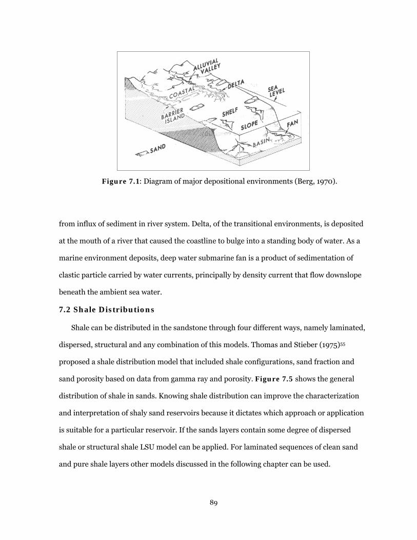
89

Figure 7.1: Diagram of major depositional environments (Berg, 1970).

from influx of sediment in river system. Delta, of the transitional environments, is deposited

at the mouth of a river that caused the coastline to bulge into a standing body of water. As a

marine environment deposits, deep water submarine fan is a product of sedimentation of

clastic particle carried by water currents, principally by density current that flow downslope

beneath the ambient sea water.

7.2 Shale Distributions

Shale can be distributed in the sandstone through four different ways, namely laminated,

dispersed, structural and any combination of this models. Thomas and Stieber (1975)55

proposed a shale distribution model that included shale configurations, sand fraction and

sand porosity based on data from gamma ray and porosity. Figure 7.5 shows the general

distribution of shale in sands. Knowing shale distribution can improve the characterization

and interpretation of shaly sand reservoirs because it dictates which approach or application

is suitable for a particular reservoir. If the sands layers contain some degree of dispersed

shale or structural shale LSU model can be applied. For laminated sequences of clean sand

and pure shale layers other models discussed in the following chapter can be used.

90

Figure 7.2: Strata characteristics of rock deposited in fluvial-meandering system (from Selley, 1976).

91

Figure 7.3: Strata characteristics of rock deposited in a wave-dominated delta system (from van Wagoner, 2003).

Figure 7.4: Strata characteristics of rock deposited in deep water sub-marine fan system (from Walker, 1975).

92

Figure 7.5: Shale distribution model based on volume of shale (Vsh) calculated from gamma ray and porosity logs data.

7.3 Resistivity Anisotropy Models

In thin bed sand shale sequences, resistivity measurement represents a significant

challenge because in many stratified rocks electric current has a favorable flow path in a

direction parallel to the bedding compared to transversely to them. The reason for this

behavior is that a great number of mineral crystals possess a flat or elongated shape (mica,

kaolinite, etc.). At the time of deposition, they were laid down with an orientation parallel to

the sedimentation strata.

Resistivity anisotropy (sometime it is called the "macroscopic anisotropy") occurs from

alternating thin beds or laminations of differing resistivity, where the individual bed

thickness are less than the resolution of the resistivity tools56. Figure 7.6 shows the limited

vertical resolution of induction logging tool compare with the thin bed thickness meaning it

measures the apparent resistivity which is a weighted average of resistivity of layers with a

Laminated shale

Structural shale

Disp

ersed sh

ale

Vsh

φsh

φmax

φ tota

l

Laminated shale

Structural shale

Disp

ersed sh

ale

Vsh

φsh

φmax

φ tota

l

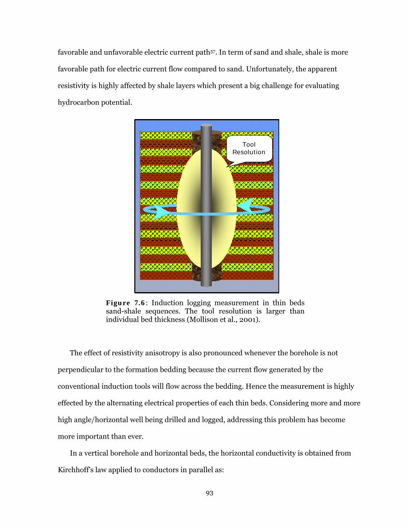
93

favorable and unfavorable electric current path57. In term of sand and shale, shale is more

favorable path for electric current flow compared to sand. Unfortunately, the apparent

resistivity is highly affected by shale layers which present a big challenge for evaluating

hydrocarbon potential.

Figure 7.6: Induction logging measurement in thin beds sand-shale sequences. The tool resolution is larger than individual bed thickness (Mollison et al., 2001).

The effect of resistivity anisotropy is also pronounced whenever the borehole is not

perpendicular to the formation bedding because the current flow generated by the

conventional induction tools will flow across the bedding. Hence the measurement is highly

effected by the alternating electrical properties of each thin beds. Considering more and more

high angle/horizontal well being drilled and logged, addressing this problem has become

more important than ever.

In a vertical borehole and horizontal beds, the horizontal conductivity is obtained from

Kirchhoff’s law applied to conductors in parallel as:

Tool Resolution

Tool Resolution

Tool Resolution

94

shshsdshh CVC)V1(C +−= [7.1]

Because the shale conductivity (Csh) is much higher than sand conductivity (Csd), the

overall horizontal conductivity (Ch) is highly affected by shale.

The ultimate goals of resistivity anisotropy evaluation in thin-bedded sand-shale

reservoir are to determine the water saturation (Sw), hydrocarbon pore volume (HPV) and a

best possible estimation of economic cut-off value for a given reservoir. To achieve these

goals, two parameters are required: 1) a representative "true resistivity" for each sand layer

(Rsand) and 2) choosing an appropriate model for Sw prediction.

Applying an incorrect method to determine true resistivity in thinly bedded reservoir

might cause underestimating the overall hydrocarbon potential to as high as 40 percent58.

Therefore, numerous models were introduced to address the resistivity anisotropy problem.

Recognition of horizontal and vertical resistivity effect on tool measurement log evaluation,

borehole geometry, effect of water saturation, shale anisotropy, and resistivity tensors

measurement has become the central idea to better characterization of the anisotropy of thin-

bed reservoirs.

Schlumberger et al. (1933)59 observed that the resistivity measured with a system of

electrodes aligned perpendicularly to the bedding planes is equal to the longitudinal

resistivity (paradox of anisotropy). In a case of an interval consisting of two thin,

homogeneous, isotropic layers, the resistivity propagates parallel (Rh) and perpendicular (Rv)

to bedding, the coefficient of anisotropy (λ) are given, respectively, by:

2

2

1

1

h

21

Rh

Rh

Rhh

+=+

[7.2]

221121v h.Rh.R)hh(R +=+ [7.3]

h

v

RR

=λ [7.4]

where h1, h2, R1, and R2 are the respective thickness and resistivity of each layers.

95

The assumptions are the measuring device is generally vertical, formation dip is small and

electrode spacing is large enough for the effect of the borehole to be negligible.

Poupon,et al. (1954)60 considered shaly sand as discrete layers of laminated sand and

shale. Therefore the volumetric fraction of each component contributed to the overall

measured resistivity. Each sand and shale contribution is measured in a parallel circuit

relationship, expressed as:

lamsh

lamsh

sand

lamsh

t RV

R.F)V1(

R1

−

−− +−

= [7.5]

where:

Rt = resistivity of reservoir rock, ohm.m

Vsh-lam = volume of laminated shale, fraction

F = formation resistivity factor

Rsand = resistivity of laminated sand, ohm.m

Rsh-lam = resistivity of laminated shale, ohm.m

Tabarovsky (1979)61 used an induction tool similar to dip meter where the transmitter

and receiver antenna were aligned perpendicular to the logging axis to derive the log

response in an anisotropic formation.

⎭⎬⎫

⎩⎨⎧

−βθ

+= )1(sin

21CC

2Hlog [7.6]

where: Clog = apparent conductivity measured, mho/m

CH = conductivity in horizontal axis, mho/m

and:

θα+θ=β 222 sincos [7.7]

V

H

H

V2

RR

CC

==α [7.8]

96

The assumption for this approach is that to get the true vertical conductivity, the induction

tools have to be perpendicular to the borehole axis.

Moran and Gianzero (1979)62 indicated the effect of formation anisotropy on resistivity

logging measurement where the borehole axis is not perpendicular to the bedding planes. In

homogeneous anisotropic formation, both induction and lateralog resistivity (Rlog) tools

measures:

αλ+α

λ=

222

Hlog

cossin

R.R [7.9]

where α and λ are, respectively, the bed inclination (dip) and coefficient of anisotropy:

H

V

V

H2

RR

=σσ

=λ [7.10]

In a case where a vertical well penetrate a horizontal formation (α = 0o), Rlog = RH.

Klein (1996)63 introduced a simple calculation of the coefficient of anisotropy as a

function of saturation for laminated formation dominated by macroporous and microporous

layer. Hence, it has general application to formation with vertical variability in capillarity.

Using the analogy that the resistivity of sand layers (Rsand) varies with hydrocarbon saturation

the anisotropy of sand-shale layers should also vary with saturation.

M

nw

m

wM

m

nw

m

wmv

S.

R.a.V

S.

R.a.VR ⎟

⎟⎠

⎞⎜⎜⎝

⎛

φ+⎟

⎟⎠

⎞⎜⎜⎝

⎛

φ= [7.11]

M

nw

m

w

M

m

nw

m

w

mh

S.

R.a

V

S.

R.a

VR

⎟⎟⎠

⎞⎜⎜⎝

⎛

φ

+

⎟⎟⎠

⎞⎜⎜⎝

⎛

φ

= [7.12]

where M and m denote, respectively, macroporous and microporous layer, and V is the

volume fraction (Vm + VM = 1). The assumption is the formation composed of alternating

parallel layers of rocks where each layer dominated by either macroporosity or microporosity.

Hagiwara (1997)64 stated the sand-layer resistivity can be estimated from the anisotropic

(log) resistivity provided shale-layer resistivity, Vsd/Vsh ratio and relative layer dip data.

97

Shale-layer resistivity can be obtained from massive shale section above or below the

laminated sequence. The sand fraction (Vsd) can be estimated from cores, imaging tools, or

high frequency dielectric tools.

shH

shVHsd RR

RR.RR

−−

= [7.13]

If the shale layers are also microscopically anisotropic, the equation is modified to:

1

H,sh

V,sh

H,sh

osd

2

H,sh

osd

H,sh

osdo

sdsd 1R

R

RR4

1RR

1RR

21

1RR

−

⎪⎭

⎪⎬

⎫

⎪⎩

⎪⎨

⎧

⎥⎥⎥

⎦

⎤

⎢⎢⎢

⎣

⎡

⎟⎟⎠

⎞⎜⎜⎝

⎛−+⎟

⎟⎠

⎞⎜⎜⎝

⎛−−−+= [7.14]

where: V,shsd

V,shVsd RR

RRV

−

−= [7.15]

and:

H,shH

V,shVH

osd RR

RR.RR

−

−= [7.16]

The assumption is that all sand layer and shale layer in the sequence is identical to each

other.

Tabanou (1999)65 proposed a method of using Rv, Rh and input for the resistivity of the

shale laminations to derive the resistivity of the clean sand layers and the net-to-gross ratio.

Rv and Rh inversion requires the apparent formation dip defined as the angle between the

normal to the bedding plane and the borehole

( )

⎟⎟⎠

⎞⎜⎜⎝

⎛−

⎟⎟⎠

⎞⎜⎜⎝

⎛−−−⎟⎟

⎠

⎞⎜⎜⎝

⎛−+⎟⎟

⎠

⎞⎜⎜⎝

⎛−

=

ho

hovo

2

h

o

o

v

h

o

o

v

sand

R1

R1

2

R1

R1

RR4RR

RR

RR

RR

R [7.17]

⎟⎟⎠

⎞⎜⎜⎝

⎛−−+

⎟⎟⎠

⎞⎜⎜⎝

⎛−−+

=

oo

sandsand

hv

sandsand

o

R1

RR

1R

R1

RR

1R

V [7.18]

Silt model: Rweq = Rw ; Shale model: Ro = Rsh

98

sand

2w

w R.

RS

φ= [7.19]

)S1()V1(V wohyd −−φ= [7.20]

The assumptions are: 1). a single water resistivity (Rwo) controls the resistivity of shale and

silt. Rwo = Rw (connate water in silt) = bound water resistivity in shale; 2). Porosity of sand is

the same as the porosity of low resistivity layers (silt and shale).

All resistivity anisotropy models discussed above concur the importance of acquiring the

information of horizontal (Rh) and vertical resistivity (Rv) to evaluate the thinly bedded

reservoirs. While Rh can be determined from conventional induction tool, the common

practice to determine Rv is using some high resolution logging tools that have a compatible

vertical resolution with the thin beds. These tools are formation micro-imager (FMI),

dipmeter, microlog, and high frequency dielectric, etc. However, because of theirs shallow

depth of investigation so that they are very sensitive to borehole condition and mud invasion,

these tools can not be used to evaluate the important properties such as resistivity and water

saturation of thin beds.

7.4. Rh and Rv Prediction

As discusses in the previous literatures addressing resistivity anisotropy requires the

information of vertical resistivity (Rv). Conventional induction tools (HDIL) only provide the

horizontal resistivity (Rh). Therefore, new multi-component resistivity tools, cost few times

more expensive than the old one, were developed to provide both Rv and Rh. The question

now is whether it is worthwhile to run this new tool at all? Or is there any additional

information that can be extracted from the conventional tool?

In vertical borehole and horizontal beds, the conventional induction tool (HDIL) is

measuring the horizontal resistivity (Rh); hence, it should give a similar Rh value as the multi-

component's (3DEX) Rh run in the same interval provided both were compared in the same

vertical resolution. Since Rh from HDIL measurement has a higher vertical resolution, a

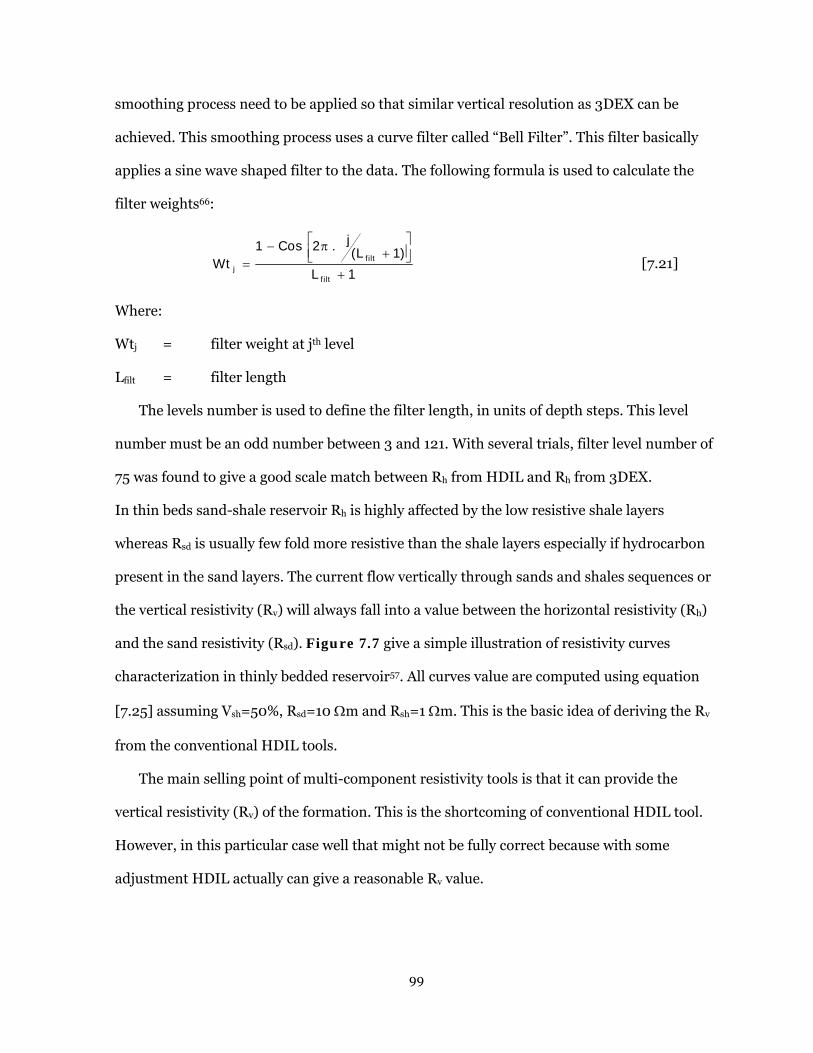
99

smoothing process need to be applied so that similar vertical resolution as 3DEX can be

achieved. This smoothing process uses a curve filter called “Bell Filter”. This filter basically

applies a sine wave shaped filter to the data. The following formula is used to calculate the

filter weights66:

1L

)1L(j.2Cos1

Wtfilt

filtj +

⎥⎦⎤

⎢⎣⎡

+π−= [7.21]

Where:

Wtj = filter weight at jth level

Lfilt = filter length

The levels number is used to define the filter length, in units of depth steps. This level

number must be an odd number between 3 and 121. With several trials, filter level number of

75 was found to give a good scale match between Rh from HDIL and Rh from 3DEX.

In thin beds sand-shale reservoir Rh is highly affected by the low resistive shale layers

whereas Rsd is usually few fold more resistive than the shale layers especially if hydrocarbon

present in the sand layers. The current flow vertically through sands and shales sequences or

the vertical resistivity (Rv) will always fall into a value between the horizontal resistivity (Rh)

and the sand resistivity (Rsd). Figure 7.7 give a simple illustration of resistivity curves

characterization in thinly bedded reservoir57. All curves value are computed using equation

[7.25] assuming Vsh=50%, Rsd=10 Ωm and Rsh=1 Ωm. This is the basic idea of deriving the Rv

from the conventional HDIL tools.

The main selling point of multi-component resistivity tools is that it can provide the

vertical resistivity (Rv) of the formation. This is the shortcoming of conventional HDIL tool.

However, in this particular case well that might not be fully correct because with some

adjustment HDIL actually can give a reasonable Rv value.

100

Rearranging the equation [7.5] yield an estimation of sand resistivity (Rsd) as a function of

the volume of shale (Vsh), resistivity of shale (Rsh), and the true resistivity (Rt) measured by

conventional induction tools (HDIL). This equation is expressed as:

shtsh

shtshsd R.RR

)V1(.R.RR

−−

= [7.22]

Volume of shale (Vsh) can be estimated using several log data such as gamma-ray and

porosity logs. Resistivity of shale (Rsh) can be determined from adjacent thick shale, and the

true resistivity (Rt) in this case where the borehole is vertical and the beds are horizontal is

equal to the horizontal resistivity (Rh). Hence, resistivity of sands (Rsd) can be calculated

using equation [7.22].

Figure 7.7: Illustration of resistivity measurement in thinly bedded sand-shale sequences. The Rv value is always between Rh and Rsand (Mollison el al., 2001).

The value of Rv between Rh at lower end and Rsd at higher end is a function of the

thickness of the sand-shale sequences. Whenever the sequences contain thicker sand and

shale layers then Rv value will move closer to Rh value since Rh is highly affected by shale. In

101

contrary, Rv value will move closer to Rsd value whenever the sequences are thinner. Since the

reservoirs in this south Texas well are considered to be thinly bedded, hence assuming Rsd

value computed from equation [7.22] is similar to that of Rv value is a good starting point. In

fact, the first run for both A sands and B sands shows that the calculated Rsd value is in the

same magnitude with Rv value from the 3DEX tools. Further fine-tuning of the input

parameters such as Vsh and Rsh based on a more specific interval of the reservoir yield a better

correlation. The calculated Rsd is still in HDIL high vertical resolution scale, so similar

smoothing process using a bell shape filter with 75 filter levels was applied to get a

derived Rv.

Figure 7.8 and Figure 7.9 show the result of predicting the horizontal (Rh) and vertical

resistivity (Rv) based only on HDIL measurement. DFZZ and DFXX curves are horizontal and

vertical resistivity measured by 3DEX tool, respectively. M2RX curve is the deep resistivity

measured by HDIL tool whereas DFZZ_HDIL and DFXX_HDIL are, respectively, horizontal

and vertical resistivity derived from HDIL tool.

The derived Rh and Rv from HDIL tools in B sands seems to have better match to the Rh

and Rv measured by 3DEX tools compare with the derived values in A sands. This outcome

really depends on the assumption used on the sand-shale sequences thickness. There is a

need to evaluate the thickness distribution in order to assess the match quality. Figure 7.10

and Figure 7.11 shows the general sand-shale thickness determined from combination of

gamma-ray, resistivity and density logs. The average of sand-shale thickness in A sands are 3

– 4 feet, where as in B sands are 1 – 2 feet. This indicated that conventional induction tool

(HDIL) used for deriving the Rh and Rv can resolve the thinner layers in B sands much better

than the thicker layers of A sands. In thinner layers, the electrical effect of shale has been

significantly reduced so that the values of vertical resistivity (Rv) measured by HDIL tools are

closer to the true formation resistivity (Rsand). Hence, deriving Rv from HDIL tools in a

102

vertical borehole with horizontal beds shows a good match with Rv measured by multi-

component resistivity tools (3DEX).

This observation seems opposite with the common believe that HDIL tool resolve rock

resistivity better in thicker sands. However, there is a scale issue different between these two

cases with respect to the tools vertical resolution. In thinly bedded cases where resistivity

anisotropy occurs, each point of HDIL tool measurement represents a sequence of sand and

shale layers. Hence, this point is highly affected by volume of shale in the sequence. As an

illustration, HDIL tool is measuring two sequences of sand and shale layers.

Figure 7.8: The comparison of derived Rh and Rv from HDIL data to the Rh and Rv from 3DEX multi-component induction tool in A sands.

103

Assuming both sequences have similar value of Rsd=10 ohm-m and Rsh=1 ohm-m, but

sequence one contain Vsh=0.5 and sequence two contain Vsh=0.2. Using equation [7.5] the

calculated Rt values for sequence one and two are 1.8 ohm-m and 3.6 ohm-m, respectively.

This example shows that by reducing the sequences thickness especially in shale layers

increase the measured formation resistivity (Rt) closer to the actual Rsd value.

Figure 7.9: The comparison of derived Rh and Rv from HDIL data to the Rh and Rv from 3DEX multi-component induction tool in B sands.

104

Figure 7.10: Thickness distribution of the thinly bedded sand and shale sequences in A sands.

Figure 7.11: Thickness distribution of the thinly bedded sand and shale sequences in B sands.

0

2

4

6

8

10

12

14

16

18

Fre

quency

1 3 5 7 9 11 13 15 17 19

Thickness (Feet)

0

10

20

30

40

50

60

70

80

90

Fre

quency

1 3 5 7 9 11 13 15 17 19

Thickness (Feet)

105

7.5 Field Applications

In order to evaluate the impact of resistivity anisotropy in calculating the hydrocarbon

pore volume (HPV) of thinly bedded reservoirs, a well data from south Texas was used. This

vertical well penetrate two main sands namely A sand and B sand. These sands were known

to have laminated layer characteristics. A suite of conventional logging tools that included

gamma ray, array induction (HDIL), and porosity tools such as density and neutron was run

in conjunction with the new tri-axial induction tools (3DEX) tools.

Hydrocarbon pore volume (HPV) calculated from different resistivity anisotropy models

are compared to each other. A water saturation cutoff of 75%, porosity cutoff of 12% and Vsh

cutoff of 50% were used in the HPV calculation. The HPV is calculated as the oil saturation

(1-Sw), times porosity (φ), times net oil thickness (h).

7.5.1 Application of Conventional Induction Tools

In thick and clean sandstone reservoirs, the deep reading of the conventional induction

tools (HDIL) is usually used to estimate the fluid saturation using Archie’s model because it

has a value close to the true formation conductivity. However, this approach has often been

extrapolated in thinly bedded reservoirs where resistivity anisotropy occurs.

In a vertical borehole and horizontal beds, the conventional induction tools (HDIL) is

measuring the horizontal conductivity of the formation. If the horizontal beds are consist of

thinly bedded sand-shale sequences then overall horizontal conductivity is a product of the

weighted-average of conductivity contribution of sand and shale layers within the tools

vertical resolution.

shshsdshh C.VC)V1(C +−= [7.23]

Because the shale conductivity (Csh) is much higher than sand conductivity (Csd) the

horizontal conductivity (Ch) will reflect more the shale component compare to the sand

component. As a result, the higher Ch will cause a higher estimation of water saturation or in

other words it will overlook of the hydrocarbon potential. To illustrate this point, water

106

saturation (Sw) calculation was done in both reservoir sands of the case well using Archie

clean sand model and Poupon laminated shale model. The result is shown in Figure 7.12

and Figure 7.13. Track one contains gamma-ray, total porosity and volume of shale. Track

two is the depth scale and track three is the deep induction curve from HDIL. Track four and

five is the calculated water saturation using Archie and Poupon’s method, respectively.

More hydrocarbon potential zones were identified by poupon laminated model compare

to Archie’s clean sand model. In other words, ignoring the laminated features of the thinly

bedded sand-shale reservoirs, the fluid saturation calculation might leave out some

hydrocarbon potential zones. In term of the calculation of hydrocarbon pore volume (HPV),

the comparison is shown in Figure 7.14 where additional HPV in A sands and B sands are

86% and 47%, respectively.

7.5.2 Application of Multi-Component Resistivity Tools

The evaluation of hydrocarbon potential in thinly bedded sand-shale reservoir depend to

a great extend on which model is used. The result from hydrocarbon pore volume (HPV)

calculation using model such as Archie’s clean sand and Poupon’s laminated shaly sand in the

case well indicated a significant potential different where the later model identified more

potential. However, this laminated model quite often still can not fully address the resistivity

anisotropy issue due to the fact that it is still using the resistivity log from conventional tools

such as HDIL that measures horizontal resistivity only (Rh).

There are many resistivity anisotropy models available in the industry and most of them

show a need of acquiring both horizontal and vertical resistivity data in thinly bedded sand-

shale reservoir. In fact, these two parameters play a key role in analyzing a reservoir where

resistivity anisotropy occurs. Hence, many oil service companies were trying to develop some

new resistivity tools that have the ability to acquire both Rh and Rv.

In a vertical borehole drilled perpendicular with the bed layer, the conventional induction

logging tools which incorporate Z-axis transmitter and receiver coil arrays generated

107

Fig

ure

7.1

2: W

ater

sat

ura

tion

est

imat

ion

usi

ng

Arc

hie

’s c

lean

san

d m

odel

an

d P

oup

on’s

lam

inat

ed s

hal

e m

odel

in A

san

ds.

108

Fig

ure

7.1

3: W

ater

sat

ura

tion

est

imat

ion

usi

ng

Arc

hie

’s c

lean

san

d m

odel

an

d P

oup

on’s

lam

inat

ed s

hal

e m

odel

in B

san

ds.

109

Figure 7.14: HPV calculation using Archie's clean sand model and Poupon's laminated shale model in A sands and B sands.

a current flow parallel to the bed layer. In this condition, the tool is measuring the horizontal

resistivity (Rh). In order to measure the vertical resistivity, additional X-axis and Y-axis need

to be incorporated. Developed by BakerAtlas, the new 3D Explorer (3DEX) induction logging

tools or tri-axial induction tools (Figure 7.15) have incorporated additional X-axis and Y-

axis coil arrays that are orthogonal to the Z-axis array along the tool axis. While the Z-axis

measurement (horizontal resistivity) is highly affected by the conductive shale, the X-axis

and Y-axis coils create an electric current flow vertical to the bedding and very sensitive to

the resistivity of hydrocarbon-bearing sands. Other oil service company such as

Schlumberger is also their own set of multi-component resistivity tools.

0.496 0.923

11.553

16.934

0

2

4

6

8

10

12

14

16

18

HPV (

Feet)

1 2

ArchiePoupon

A Sand B Sand

0.496 0.923

11.553

16.934

0

2

4

6

8

10

12

14

16

18

HPV (

Feet)

1 2

ArchiePoupon

A Sand B Sand

110

Figure 7.15: Multi-component measurement in three orthogonal directions performed by 3DEX tool to get the horizontal and vertical resistivity (Mollison, et al., 2001).

To evaluate the impact of having Rh and Rv in HPV calculation in thinly bedded reservoir

where resistivity anisotropy occurs, four anisotropy models discussed previously were used.

These models are Hagiwara shale-isotropy model, Hagiwara shale-anisotropy, Tabanou

model and Tabarovsky model. The main reason to select these models is because they

represent a wide spectrum of model used by major oil service companies. All models differ

only in which sand resistivity (Rsand) is used in the general Archie’s water saturation equation.

Figure 7.16 and Figure 7.17 shows the result of water saturation calculated from those

four models. Track one contain of log data such as gamma ray (GR), volume of shale (VCL)

and total porosity (PHIT). Track two is depth scale and track three contain deep resistivity

log (M1RX), horizontal resistivity (DFZZ) and vertical resistivity (DFXX). Track four

contains sand resistivity logs calculated using different resistivity anisotropy models. They

are sand resistivity determined from Hagiwara isotropic shale (Rsd_Hagi), Hagiwara

anisotropic shale (Rsd_Hagi1), Tabanou (Rsd_Tbn) and Tabarovsky (Rsd_Tbo). Track five to

eight are calculated water saturation using the resistivity anisotropy model discussed above.

111

Taking into account the resistivity anisotropy effect by incorporating Rh and Rv in the

formation evaluation of thinly bedded sand-shale reservoir has a significant impact on

identifying hydrocarbon potential. In term of hydrocarbon pore volume (HPV), Figure 7.18

and Figure 7.19 show the comparison of all models including Archie’s and Poupon’s model.

All HPV calculation is limited by 75% water saturation cutoff, 12% sand porosity cutoff and

50% of volume of clay cutoff.

The estimation of water saturation and hydrocarbon pore volume using all models

(isotropy and anisotropy) indicated that ignoring the resistivity anisotropy in thin beds sand-

shale reservoir can result in missing the a vast amount of hydrocarbon potential.

7.5.3 Application of LSU Model

In thinly bedded sand-shale reservoir, the water saturation of each sand layer can be

estimated using Archie's equation:

sand

wnw R

R.FS = [7.24]

Poupon (1954) started to modify the Archie’s equation used specifically in laminated

formation by simply improving the definition of Rsand term. This new Rsand equation

incorporates the volume fraction of laminated shale (Vsh) and the resistivity of thin shale

layer (Rsh) into the equation and yield:

sh

sh

sand

sh

t RV

R)V1(

R1

+−

= [7.5]

Identifying the true resistivity of sand (Rsand) has then become the main focus of most of the

research in thinly bedded sand-shale sequence as discussed earlier in laminated shaly sand

models.

There is, however, one major assumption used in developing those models where the

sequences are consisted of thin layer of shale and clean sand. Because in clean sand layer only

one type of water is present in the pore space a constant water resistivity (Rw) is expected.

112

Fig

ure

7.1

6: W

ater

sat

ura

tion

est

imat

ion

of

A s

and

s u

sin

g fo

ur

dif

fere

nt

resi

stiv

ity

anis

otro

py

mod

els

(Hag

iwar

a is

otro

pic

sh

ale,

Hag

iwar

a an

isot

rop

ic s

hal

e, T

aban

ou a

nd

Tab

arov

sky)

.

113

Fig

ure

7.1

7: W

ater

sat

ura

tion

est

imat

ion

of

B s

and

s u

sin

g fo

ur

dif

fere

nt

resi

stiv

ity

anis

otro

py

mod

els

(Hag

iwar

a is

otro

pic

sh

ale,

Hag

iwar

a an

isot

rop

ic s

hal

e, T

aban

ou a

nd

Tab

arov

sky)

.

114

Figure 7.18: Hydrocarbon pore volume (HPV) calculated in A sands using various resistivity isotropy and anisotropy models.

Figure 7.19: Hydrocarbon pore volume (HPV) calculated in B sands using various resistivity isotropy and anisotropy models.

0.923

1.011

10.01

15.41

19.04

0 5 10 15 20 25 30

POUPON

TABAROVSKY

HAGIWARA

HAGIWARA1

TABANOU

HPV (Feet)

16.93

18.88

37.44

51.55

51.16

0 10 20 30 40 50 60

POUPON

TABAROVSKY

HAGIWARA

HAGIWARA1

TABANOU

HPV (feet)

115

This Rw usually can be estimated in water-bearing clean sand using SP log or chemical

analysis of the produced water sample. Therefore, the value of Rw value is assumed to be

unique and depend only on temperature and salinity of the formation

This assumption, however, does not represent well with the actual reservoir

characteristics where most of hydrocarbon-bearing sands contain both laminated and

dispersed shale67. Therefore, addressing the resistivity anisotropy in shaly sand, which closely

related to the type and distribution of the shale using only laminated

approach, will prone to some incorrect estimation of the rock properties. In addition, the

isotropic assumption in the individual sands does not represent well the common sandstone

characteristics.

A new approach is proposed to evaluate the impact of resistivity anisotropy to the

hydrocarbon pore volume estimation by taking into account the distribution of shale in both

laminated and dispersed form. Laminated form means exactly like the previous assumption

where the sequences consist of thin shale and clean sands. While dispersed means that each

sand and shale is macroscopically laminated but individual sand has some degree of

dispersed shale.

Consequently, in dispersed form Archie’s equation [7.24] can be improved not only by

modifying Rsand but also Rw. Because dispersed shaly sand consists of a mixture of free water

and bound water, LSU models can be used to evaluate the correct mixture water resistivity

(RwM). LSU model uses the dual-water principle where shaly sand consists of two types of

water, bound water and free water. The overall water resistivity, thus, is a mixture of both

type of water. In term of mixture water conductivity (CwM), LSU model can be expressed as:

FwfdleqeqfdlMw C.)v1(n.c.vC −+= [7.25]

Where:

vfdl = volume of double layer, fraction

ceq = equivalent counterion conductivity, mho/m

116

neq = equivalent counterion concentration, mol/l

CwF = free water conductivity, mho/m

To verify the assumption that individuals sand layers contain some degree of dispersed

shale, Thomas-Stieber shale distribution model was used to evaluate A sand and B sand.

Figure 7.20 and Figure 7.21 indicated dispersed shale characteristics in most of thin sand

layers.

Shale distribution in A sands are mainly dispersed while in B sands there are some degree

of laminated shale distribution. The overall A sands consist of thicker sand layer compare to

B sands. In geological sense it means A sands were form in longer deposition time than B

sands hence there was higher possibility to get disturbed either by weather or media

transport energy (e.g., water current) where finer particles such as shale and clay could mixed

with other sandstone matrix such as quartz.

Figure 7.20: Indication of dispersed shale distribution in thin sand layers in A sands.

φmax

φsh

Laminated

Disp

ersed

φmax

φsh

φmax

φsh

Laminated

Disp

ersed

117

Figure 7.21: Indication of dispersed shale distribution in thin sand layers in B sands.

Since shale is dispersedly distributed in thin sands layer LSU model can be applied. This

model is mainly used to determine the mixture water conductivity (CwM) in order to calculate

the water saturation using Archie’s equation. The calculation process using LSU model is

discussed in detail in chapter 3. To determine the mixture water resistivity, the procedures

are as follow:

1. Computed all the preliminary parameters such as temperature, neq, ceq, fdl and vQ.

2. Determine the cementation exponent of the free water (mf) in adjacent clean sand and

cementation exponent of bound water (mc) in adjacent thick shale.

3. The cations exchange capacity (Qv) in shaly sand can be determined in a wet shaly

sand interval where the formation conductivity is measured. Based on LSU model, the

conductivity of a fully-brine saturated interval (Co) can be expressed as:

wFmfmf

fdlmcmc

fdleqeqo C..)v1(.v.c.nC φ−+φ= [3.44]

where

vQdlfdl Q.v.fv = [3.21]

φsh

φmaxLaminated

Disp

ersed

φsh

φmaxLaminated

Disp

ersed

118

Assuming Qv value is similar in each thin-sand layers, the mixture water conductivity (CwM)

can be computed using equation [7.25]. In this south Texas case well, log data from a wet

shaly sand section was used to calculate Qv. The preliminary parameters calculated in this

section are neq= 8.1764 mol/l; ceq=3.6134 mho/m. Data determined from logs are average

porosity (�)=0.16 and fully-brine saturated shaly sand (Co)= 0.625 mho/m. Data from

chemical analysis is free water conductivity (CwF) = 25 mho/m. While mc and mf were

determined using cross-plot of porosity and formation resistivity factor (F) in adjacent thick

shale and clean sand, respectively (Figure 7.22).

LSU model enables the computation of mixture water conductivity (CwM) in thinly bedded

sand-shale reservoir provided the thin sand layer contains some degree of dispersed shale.

The calculation of CwM using equation [7.25] and equation [3.44] yield a value of CwM=29

mho/m and a value of Qv = 1.44 meq/l. The new water saturation values using these

parameters were calculated based on Archie equation. These Sw values are lower than Sw

value calculated using existing anisotropy model (Figure 7.23 and Figure 7.24). This

means more hydrocarbon potential can be identified using LSU model.

In term of hydrocarbon pore volume (HPV), 6%-80% of additional potential can be

determined as shown in Figure 7.25 and Figure 7.26. Providing the assumption, thin

sands layer contain dispersed shale, is met, LSU model can improve the evaluation of thinly

bedded sand-shale reservoir where resistivity anisotropy occurs.

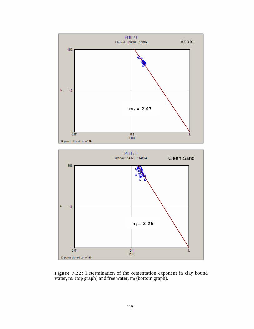
119

Figure 7.22: Determination of the cementation exponent in clay bound water, mc (top graph) and free water, mf (bottom graph).

ShaleShaleShaleShaleShaleShaleShaleShale

mc = 2.07

Clean SandClean SandClean Sand

mf = 2.25

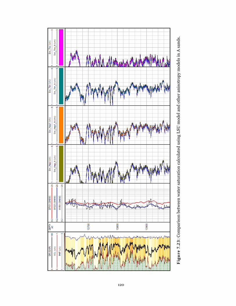
120

Fig

ure

7.2

3: C

omp

aris

on b

etw

een

wat

er s

atu

rati

on c

alcu

late

d u

sin

g L

SU

mod

el a

nd

oth

er a

nis

otro

py

mod

els

in A

san

ds.

121

Fig

ure

7.2

4: C

omp

aris

on b

etw

een

wat

er s

atu

rati

on c

alcu

late

d u

sin

g L

SU

mod

el a

nd

oth

er a

nis

otro

py

mod

els

in B

san

ds.

122

Figure 7.25: Additional HPV determined using LSU model in A sands reservoir on top of HPV determined from other anisotropy models.

Figure 7.26: Additional HPV determined using LSU model in B sands reservoir on top of HPV determined from other anisotropy models.

0

10

20

30

40

50

60

HPV

(Fe

et)

TABAROVSKY HAGIWARA HAGIWARA1 TABANOU

Original HPV Additional HPV

0

5

10

15

20

25

HPV

(Fe

et)

TABAROVSKY HAGIWARA HAGIWARA1 TABANOU

Original HPV Additional HPV

123

CHAPTER 8 CONCLUSIONS AND RECOMMENDATIONS

Experimental measurement on actual reservoir rock samples taken from South Louisiana

well where high degree of shaliness occurs has been conducted to validate the latest LSU

model. This model incorporated two different formation resistivity factors to represent the

tortuosity of electric current flow in free water and clay bound water in dispersed shaly sand.

The result shows a better characterization of electrical properties of shaly sand using two

formation resistivity factors estimated from representative adjacent clean sand and pure

shale interval compared to the current practice of using only one formation resistivity factor

estimated in shaly sand interval.

Uncertainty analysis of LSU shaly sand model using Monte Carlo simulation indicates

that the formation conductivity (Ct), total porosity (φt), and cations exchange capacity (Qv)

are among the most sensitive parameters in water saturation (Sw) calculation using LSU

model. Assuming input parameters (Ct and φt) were uncorrelated will cause the sensitivity of

Sw to Ct become negligible.

From the electrical properties measurement of the same shaly sand samples from South

Louisiana and the measurement of their cations exchange capacity (Qv) value, two

correlations between saturation exponent of shaly sand and Qv have been constructed. These

correlations are for water salinities below and above 15,000 ppm, respectively.

124

This study defined a new technique to calculate effective porosity using gamma-ray,

neutron and density logging data. In addition, this new technique also allows the estimation

of cations exchange capacity (Qv) simultaneously with its corresponding effective porosity.

This provides an alternative and independent method to estimate Qv other than the former

common method of electrical properties measurement of cores or logs data. Field application

of this method using logs and cores data from oil wells in Indonesia shows a good correlation

between calculated and measured effective porosity in zones where the predominant clays

minerals are known from other independent measurements.

The latest LSU model can be used together with other resistivity anisotropy models to

detect optimum hydrocarbon potential in thinly-bedded shaly sand reservoirs that might be

overlooked because of the effect of electrical anisotropy. This approach can is recommended

whenever some degree of dispersed shaliness occurs in the thin sands layers.

Based on experimental measurement of shaly sand samples from South Louisiana

reservoirs, the latest LSU model utilize two formation resistivity factors shows a better

representative of electrical behavior in shaly sand. More field applications in different

geographic location with varying clay types and brine salinity are recommended to further

validate this model.

The effective porosity methods which take into account different clay types effect has

been developed for liquid-filled reservoir. However, further work still need to be done in

complex gas bearing formation where gas density becomes a major factor in a porosity

model.

125

BIBLIOGRAPHY

1. Alfosail, K.A., and Alkaabi, A.U., “Water Saturation in Shaly Formation”, SPE paper 37746, presented at Middle East Oil Show, Bahrain, 15-18 March 1997.

2. Pettijohn, F.J., “Sedimentary Rocks”, Harper and Row publisher, 1975, ch.8. 3. Clavier, C., Coates, G., and Dumanoir, J., 1984, “Theoretical and Experimental Bases for

the Dual-Water Model for Interpretation of Shaly Sands”, SPE Journal, v.24, no.2, p. 153-168.

4. Syngaevsky, P., 2000, “Shaly Sand Models: a Review”, Louisiana State University. 5. Schlumberger Educational Services, 1989, “Log Interpretation Principles/Applications”. 6. Poupon, A., Clavier, C., Dumanoir, J., Gaymard, R., and Misk, A., 1970, “Log Analysis of

Sand-Shale Sequences-A Systematic Approach”, Journal of Petroleum Technology, v. 22, p. 867-881, July, 1970.

7. Worthington, P.F., “Evolution of Shaly-Sand Concept in Reservoir Evaluation”, The Log

Analyst, v.26, no.1, 1985, pp.23-40. 8. Archie, G.E., “The Electrical Resistivity Log as an Aid in Determining some Reservoir

Characteristics”, Trans. AIME, v.146, p.54-62, 1942. 9. Simandoux, P., 1963, “Dielectric Measurements on Porous Media: Application to

Measurement of Water Saturation: Study of the Behavior of Argillacious Formation”, SPWLA, Houston, p. IV 97-124.

10. Poupon, A., and Leveaux, J., 1971, “Evaluation of Water Saturations in Shaly Formation”,

The Log Analyst, July-August, p. 3-8. 11. Waxman, M. H., and Smits, L.J.M., “Electrical Conductivities in Oil Bearing Shaly

Sands”, SPE Journal 8, p.107-122, 1968. 12. Silva, P., and Bassiouni, Z., 1985, “A Shaly Sand Conductivity Model Based on Variable

Equivalent Counter-ion Conductivity and Dual Water Concepts”, SPWLA Trans., paper RR, 1985.

13. Lau, M., 1989, “Development and Field Applications of Shaly Sand Petrophysical

Models”, Ph.D Dissertation, Louisiana State University. 14. Lau, M.N., and Bassiouni, Z., 1990, “Development and Field Applications of Shaly Sand

Petrophysical Models Part I: The Conductivity Model”, SPE paper 20386, 1990.

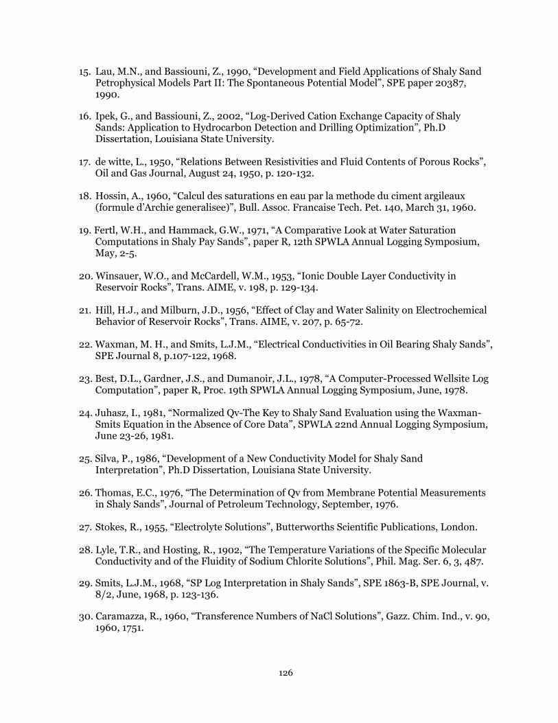
126

15. Lau, M.N., and Bassiouni, Z., 1990, “Development and Field Applications of Shaly Sand Petrophysical Models Part II: The Spontaneous Potential Model”, SPE paper 20387, 1990.

16. Ipek, G., and Bassiouni, Z., 2002, “Log-Derived Cation Exchange Capacity of Shaly

Sands: Application to Hydrocarbon Detection and Drilling Optimization”, Ph.D Dissertation, Louisiana State University.

17. de witte, L., 1950, “Relations Between Resistivities and Fluid Contents of Porous Rocks”,

Oil and Gas Journal, August 24, 1950, p. 120-132. 18. Hossin, A., 1960, “Calcul des saturations en eau par la methode du ciment argileaux

(formule d’Archie generalisee)”, Bull. Assoc. Francaise Tech. Pet. 140, March 31, 1960. 19. Fertl, W.H., and Hammack, G.W., 1971, “A Comparative Look at Water Saturation

Computations in Shaly Pay Sands”, paper R, 12th SPWLA Annual Logging Symposium, May, 2-5.

20. Winsauer, W.O., and McCardell, W.M., 1953, “Ionic Double Layer Conductivity in

Reservoir Rocks”, Trans. AIME, v. 198, p. 129-134. 21. Hill, H.J., and Milburn, J.D., 1956, “Effect of Clay and Water Salinity on Electrochemical

Behavior of Reservoir Rocks”, Trans. AIME, v. 207, p. 65-72. 22. Waxman, M. H., and Smits, L.J.M., “Electrical Conductivities in Oil Bearing Shaly Sands”,

SPE Journal 8, p.107-122, 1968. 23. Best, D.L., Gardner, J.S., and Dumanoir, J.L., 1978, “A Computer-Processed Wellsite Log

Computation”, paper R, Proc. 19th SPWLA Annual Logging Symposium, June, 1978. 24. Juhasz, I., 1981, “Normalized Qv-The Key to Shaly Sand Evaluation using the Waxman-

Smits Equation in the Absence of Core Data”, SPWLA 22nd Annual Logging Symposium, June 23-26, 1981.

25. Silva, P., 1986, “Development of a New Conductivity Model for Shaly Sand

Interpretation”, Ph.D Dissertation, Louisiana State University. 26. Thomas, E.C., 1976, “The Determination of Qv from Membrane Potential Measurements

in Shaly Sands”, Journal of Petroleum Technology, September, 1976. 27. Stokes, R., 1955, “Electrolyte Solutions”, Butterworths Scientific Publications, London. 28. Lyle, T.R., and Hosting, R., 1902, “The Temperature Variations of the Specific Molecular

Conductivity and of the Fluidity of Sodium Chlorite Solutions”, Phil. Mag. Ser. 6, 3, 487. 29. Smits, L.J.M., 1968, “SP Log Interpretation in Shaly Sands”, SPE 1863-B, SPE Journal, v.

8/2, June, 1968, p. 123-136. 30. Caramazza, R., 1960, “Transference Numbers of NaCl Solutions”, Gazz. Chim. Ind., v. 90,

1960, 1751.

127

31. Millero, F.J., 1979, “Effects of Pressure and Temperature on Activity Coefficients”, Published in Activity Coefficients in Electrolyte Solutions, CRC Press, 1979.

32. Hill, H.J., Shirley, O.J., and Klein, G.E., 1979, “Bound Water in Shaly Sands and Its

Relation to Qv and othe Formation Properties”, The Log Analyst, May-June, p. 3-19. 33. Mitchum, R.M., 1977, “Seismic Stratigraphy and Global Changes of Sea Level, Part I:

Glossary of terms used in seismic stratigraphy”, Seismic Stratigraphy-Application to Hydrocarbon Exploration, AAPG Memoir 26, p.205-212.

34. Hewlett-Packard, 1984, “Model 4276A LCZ Meter-Operation and Service Manual”,

Yokogawa-Hewlett-Packard LTD, Takakura-Cho, Hachioji-Shi, Tokyo, Japan. 35. Santamarina, J.C., Klein, K.A., and Fam, M.A., 2001, “Soils and Waves”, John Wiley and

sons, Chichester. 36. Longeron, D.G, Argaud, M.J., and Bouviever, Ll, 1989a, “Resistivity Index and Capillary

Pressure Measurements under Reservoir conditions using Crude Oil”, SPE paper 19589, 64th SPE Annual Technical Conference and Exhibition, San Antonio, TX.

37. Doveton, J.H., 1994, “Geologic Log Analysis Using Computer Methods”, AAPG Computer

Application in Geology, No.2, p. 2-3. 38. Voss, D., 1998, “Quantitative Rish Analysis”, John Wiley and Sons, New York, 328p. 39. Iman, R.L., and Conover, W.J., 1982, “A Distribution-Free Approach to Inducing Rank

Correlation Among Input Variables”, Communication is Statistics, 11(3), p. 311-334. 40. Shon, J.H., 1996, “Physical Properties of Rocks: Fundamentals and Principles of

Petrophysics”, Handbook of Geophysical Exploration, vol. 18, Pergamon Publisher. 41. Worthington, P.F. and Pallat, N., 1989, “Effect of Variable Saturation Exponent upon the

Evaluation of Hydrocarbon Saturation”, SPE paper 20538, p. 101-110. 42. Bhuyan, K., and Passey, Q.R., 1994, “Clay Estimation from GR and Neutron-Density

Porosity Logs”, paper D, SPWLA 35th Annual Logging Symposium, June 19-22, 1994. 43. Larionov, V.V., 1969, “Borehole Radiometry”, Nedra, Moskwa, 1969. 44. Stieber, S.J., 1970, “Pulsed Neutron Capture Log Evaluation in the Louisiana Gulf Coast”

SPE paper 2961, presented at the SPE Annual Meeting, Houston, October, 4-7, 1970. 45. Clavier, C., Hoyle, W.R., and Meunier, D., 1971, “Quantitative Interpretation of Thermal

Neutron Decay Time Logs: Part I-Fundamentals and Techniques”, Journal of Petroleum Technology, June, 1971, p. 743-755.

46. La Vigne, J., Herron, M., and Hertzog, R., 1994, “Density-Neutron Interpretation in Shaly

Sands”, paper EEE, 35th SPWLA Annual Logging Symposium, June 19-22, 1994. 47. Brindley, G.W., 1951, “The Kaolin Minerals: X-Ray Identification and Structure of the

Clay Minerals”, Mineralogy Society of Great Britain Monograph, p. 32-75.

128

48. Serra, O, 1984, “Fundamental of Well-log Interpretation”, Elsevier Science Publisher B.V., 1984, p. 142-143.

49. Schlumberger Ltd, 1990, “Element Mineral Rock Catalog”. 50. Schoen, J.H., Yu, L., Georgi, D.T., and Fanini, O, 2000, “Aspects of Multicomponent

Resistivity Data and Macroscopic Resistivity Anisotropy”, SPE paper 62909, SPE Annual Technical Conference and Exhibition, Dallas, TX, October,1-4, 2000.

51. Berg, R.R., 1970, “Identification of Sedimentary Environments in Reservoir Sandstones”,

Gulf Coast Ass. Of Geological Soc. Trans., v. 20, p.137-143. 52. Selley, R.C., 1976, “An Introduction to Sedimentology”, Academic Press, London. 53. van Wagoner, J.C., Mitchum, R.M., Campion, K.M., and Rahmanian, V.D., 2003,

“Siliciclastic Sequence Stratigraphy in Well Logs, Cores and Outcrops”, AAPG Methods in Exploration Series, No. 7, p. 12-13.

54. Walker, R.G., 1975, “Generalized Facies Models for Resedimented Conglomerates of

Turbidite Association”, Bull. Geol. Soc. America, v. 86, p.737-748. 55. Thomas, E.C., and Stieber, S.J., 1975, “The Distribution of Shale in Sandstones and Its

Effect upon Porosity”, paper T, SPWLA 16th Annual Logging Symposium, New Orleans, June 4-7.

56. Klein, J.D., 1993, “Induction Log Anisotropy Corrections”, The Log Analyst, vol. 34, no.2,

March-April, p. 18-27. 57. Mollison, R.A., Fannini, O.N., Kriegshauser, L., Yu, L., Ugueto, G., van Popta, J., and

Ragland, T.V., 2001, "New 3DEX induction data and tensor resistivity saturation analysis examples, Shell Ursa Field, deepwater Gulf of Mexico ", AAPG Annual meeting, 3-6 June 2001, Denver, Colorado.

58. Van den Berg, F.G., and Sandor, R.K.J., 1996, “SANDWICH: Log Evaluation in

Laminated Shaly Sands”, paper BB, SPWLA 37th Annual Logging Symposium Transactions, June 16-19.

59. Schlumberger, C., Schlumberger, M., and Leonardon, G., 1933, “Some Observations

Concerning Electrical Measurements in Anisotropic Media, and Their Interpretation”, Transaction of the American Institute of Mining and Metallurgical Engineers, vol. 97, p.367-391.

60. Poupon, A., Loy, M.E., and Tixier, M.P., 1954, "A Contribution to Electrical Log

Interpretation in Shaly Sands", Transaction of AIME, vol. 201, p. 138-145. 61. Tabarovsky, L. A., and Epov, M.I., 1979, "Geometric and Frequency Focusing for

Investigation of Anisotropic Layers in Electromagnetic Well Logging" Nauka, Siberian Division, Academy of Science, USSR, Novosibirsk.

62. Moran, J. H., and Gianzero, S., 1979, "Effects of Formation Anisotropy on Resistivity-

Logging Measurements", Geophysics, vol. 44, no. 7, July 1979, p. 1266-1286.

129

63. Klein, J. D., 1996, "Saturation Effects on Electrical Anisotropy", The Log Analyst, vol. 37, no. 1, Jan.-Feb. 1996, p. 47-49.

64. Hagiwara, T., 1997, "Macroscopic Anisotropy Approach to Analysis of Thinly Laminated

Sand/Shale Sequences: Sensitivity Analysis of Sand Resistivity Estimate and Environmental Corrections", SPE 38669, p. 275-286.

65. Tabanou, J. R., Anderson, B., Bruce, S., Bornemann, T., Hodenfield, K., and Wu, P., 1999,

"Which Resistivity Should Be Used to Evaluate Thinly Bedded Reservoirs in High-Angle Wells?", SPWLA 40th Annual Logging Symposium, May 30-June 3 1999, paper E.

66. Whitehead, F., 1997, “Interactive Petrophysic Software Manual”, Production Geoscience

Ltd, Schlumberger Information Solution. 67. Fertl, W.H., and Frost, E. Jr., 1980, “Evaluation of Shaly Clastic Reservoir Rocks”, SPE

paper 8450, Journal of Petroleum Technology, September, 1980, p. 1641-1646.

130

APPENDIX A NOMENCLATURE

131

a = Archie’s constant

B = Waxman’s equivalent counter-ion conductivity

Ccl = clay conductivity, mho-m

Ceq = equivalent counter-ion conductivity, mho-m

Ceq’ = equivalent vounter-ion conductivity for Sw < 1, mho-m

Csh = shale conductivity, mho-m

Co = conductivity of formation fully saturated with water, mho-m

Ct = formation conductivity, mho-m

Cw = water conductivity, mho-m

Cwe = equivalent water conductivity, mho-m

CwF = water conductivity in free water, mho-m

CwM = mixture water conductivity, mho-m

Em = electrochemical potential, mV

Emsh = electrochemical potential across shales, mV

Emss = electrochemical potential across shaly sand, mV

F = Faraday’s constant

F = formation factor

F* = formation factor in W-S model

Fe = formation factor in LSU model

Fo = formation factor in D-W model

fdl = expansion factor of the double layer

fg = empirical correction factor

F(ne) = empirical correction factor

GR = gamma ray log reading, API

HI = hydrogen index

HIma = hydrogen index in matrix

132

HIf = hydrogen index in fluid

HIcl* = hydrogen index in dry clay

Ish = index of shale, fraction

IR = resistivity index

m = molality, mol/Kg H2O

m = cementation exponent

mc = cementation exponent in clay bound water

mf = cementation exponent in free water

meff = membrane efficiency

n = molarity, mol/l

n = saturation exponent

n* = saturation exponent of shaly sand

neq = equivalent counter-ion concentration, mol/l

Qv = cation exchange capacity, meq/cc

Qv’ = cation exchange capacity for Sw < 1, meq/cc

Qvn = normalized cation exchange capacity

(Qv)sh= cation exchange capacity in shale

R = universal gas constant

Rh = horizontal resistivity, ohm/m

Ro = resistivity of shale/clay mixture, ohm/m

Rsh = shale resistivity, ohm/m

Rsh,h = horizontal shale resistivity, ohm/m

Rsh,v = vertical shale resistivity, ohm/m

Rsd = sand resistivity, ohm/m

Rt = formation resistivity, ohm/m

Rw = formation water resistivity, ohm/m

133

Rv = vertical resistivity, ohm/m

SP = spontaneous potential log reading, mV

Sw = water saturation, fraction

SwB = bound water saturation, fraction

T = temperature, oC

Ta = absolute temperature, oK

TNa+ = sodium transport number

tNahf = Hittorf transport number

TNash = shale transport number

TNass = shaly sand transport number

tfw = free water transport number

tw = water transport number

Vb = bulk volume

Vbw = volume of bound water

Vfw = volume of free water

Vcl* = volume of dry clay

vfdl = fractional volume of the double layer

Vsh = fractional volume of shale, fraction

vQ = amount of clay water associated with 1 unit (meq) of clay counterions

XH = 6.18 Å

α = clavier’s double layer expansion factor

β = 2.05, constant

γ± = mean activity coefficient

γ±298 = mean activity coefficient at 25oC

τ = empirical correction factor

134

ρb = bulk density, gram/cc

ρbw = density of bound water, gram/cc

ρcl* = density of dry clay, gram/cc

ρfw = density of free water, gram/cc

ρf = fluid density, gram/cc

ρma = matrix density, gram/cc

φ = porosity, fraction

φbw = volume fraction of bound water, fraction

φcl* = volume fraction of dry clay, fraction

φD = density porosity, fraction

(φD)*cl = density porosity in dry clay, fraction

φe = effective porosity, fraction

φfw = volume fraction of free water, fraction

φN = neutron porosity, fraction

(φN)*cl = neutron porosity in dry clay, fraction

φT = total porosity, fraction

135

APPENDIX B DATA OF CLEAN SAND ELECTRICAL MEASUREMENT

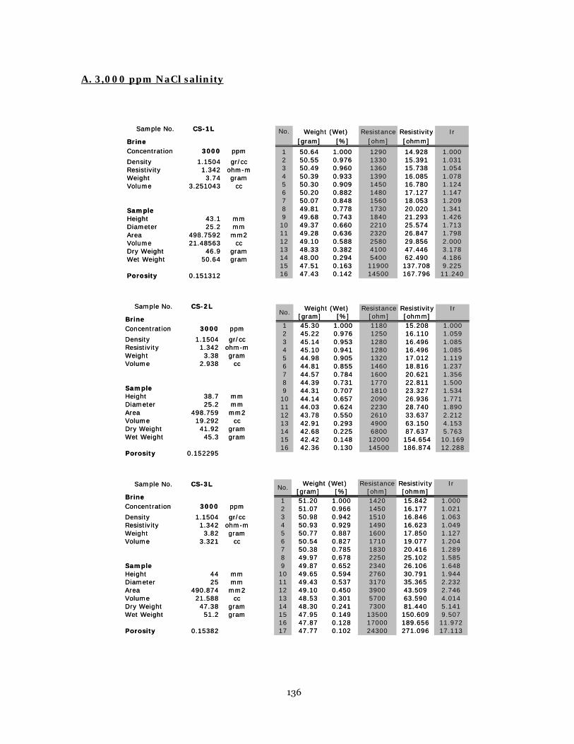
136

A. 3,000 ppm NaCl salinity

Sample No. CS-1L

Brine Concentration 3000 ppm

Density 1.1504 gr/ccResistivity 1.342 ohm-mWeight 3.74 gramVolume 3.251043 cc

SampleHeight 43.1 mmDiameter 25.2 mmArea 498.7592 mm2Volume 21.48563 ccDry Weight 46.9 gramWet Weight 50.64 gram

Porosity 0.151312

No. Resistance Resistivity Ir[gram] [%] [ohm] [ohmm]

1 50.64 1.000 1290 14.928 1.0002 50.55 0.976 1330 15.391 1.0313 50.49 0.960 1360 15.738 1.0544 50.39 0.933 1390 16.085 1.0785 50.30 0.909 1450 16.780 1.1246 50.20 0.882 1480 17.127 1.1477 50.07 0.848 1560 18.053 1.2098 49.81 0.778 1730 20.020 1.3419 49.68 0.743 1840 21.293 1.42610 49.37 0.660 2210 25.574 1.71311 49.28 0.636 2320 26.847 1.79812 49.10 0.588 2580 29.856 2.00013 48.33 0.382 4100 47.446 3.17814 48.00 0.294 5400 62.490 4.18615 47.51 0.163 11900 137.708 9.22516 47.43 0.142 14500 167.796 11.240

Weight (Wet)Sample No. CS-1L

Brine Concentration 3000 ppm

Density 1.1504 gr/ccResistivity 1.342 ohm-mWeight 3.74 gramVolume 3.251043 cc

SampleHeight 43.1 mmDiameter 25.2 mmArea 498.7592 mm2Volume 21.48563 ccDry Weight 46.9 gramWet Weight 50.64 gram

Porosity 0.151312

No. Resistance Resistivity Ir[gram] [%] [ohm] [ohmm]

1 50.64 1.000 1290 14.928 1.0002 50.55 0.976 1330 15.391 1.0313 50.49 0.960 1360 15.738 1.0544 50.39 0.933 1390 16.085 1.0785 50.30 0.909 1450 16.780 1.1246 50.20 0.882 1480 17.127 1.1477 50.07 0.848 1560 18.053 1.2098 49.81 0.778 1730 20.020 1.3419 49.68 0.743 1840 21.293 1.42610 49.37 0.660 2210 25.574 1.71311 49.28 0.636 2320 26.847 1.79812 49.10 0.588 2580 29.856 2.00013 48.33 0.382 4100 47.446 3.17814 48.00 0.294 5400 62.490 4.18615 47.51 0.163 11900 137.708 9.22516 47.43 0.142 14500 167.796 11.240

Weight (Wet)

Sample No. CS-2L

Brine Concentration 3000 ppm

Density 1.1504 gr/ccResistivity 1.342 ohm-mWeight 3.38 gramVolume 2.938 cc

SampleHeight 38.7 mmDiameter 25.2 mmArea 498.759 mm2Volume 19.292 ccDry Weight 41.92 gramWet Weight 45.3 gram

Porosity 0.152295

Resistance Resistivity Ir[gram] [%] [ohm] [ohmm]

1 45.30 1.000 1180 15.208 1.0002 45.22 0.976 1250 16.110 1.0593 45.14 0.953 1280 16.496 1.0854 45.10 0.941 1280 16.496 1.0855 44.98 0.905 1320 17.012 1.1196 44.81 0.855 1460 18.816 1.2377 44.57 0.784 1600 20.621 1.3568 44.39 0.731 1770 22.811 1.5009 44.31 0.707 1810 23.327 1.53410 44.14 0.657 2090 26.936 1.77111 44.03 0.624 2230 28.740 1.89012 43.78 0.550 2610 33.637 2.21213 42.91 0.293 4900 63.150 4.15314 42.68 0.225 6800 87.637 5.76315 42.42 0.148 12000 154.654 10.16916 42.36 0.130 14500 186.874 12.288

Weight (Wet)No.

Sample No. CS-2L

Brine Concentration 3000 ppm

Density 1.1504 gr/ccResistivity 1.342 ohm-mWeight 3.38 gramVolume 2.938 cc

SampleHeight 38.7 mmDiameter 25.2 mmArea 498.759 mm2Volume 19.292 ccDry Weight 41.92 gramWet Weight 45.3 gram

Porosity 0.152295

Resistance Resistivity Ir[gram] [%] [ohm] [ohmm]

1 45.30 1.000 1180 15.208 1.0002 45.22 0.976 1250 16.110 1.0593 45.14 0.953 1280 16.496 1.0854 45.10 0.941 1280 16.496 1.0855 44.98 0.905 1320 17.012 1.1196 44.81 0.855 1460 18.816 1.2377 44.57 0.784 1600 20.621 1.3568 44.39 0.731 1770 22.811 1.5009 44.31 0.707 1810 23.327 1.53410 44.14 0.657 2090 26.936 1.77111 44.03 0.624 2230 28.740 1.89012 43.78 0.550 2610 33.637 2.21213 42.91 0.293 4900 63.150 4.15314 42.68 0.225 6800 87.637 5.76315 42.42 0.148 12000 154.654 10.16916 42.36 0.130 14500 186.874 12.288

Weight (Wet)No.

Sample No. CS-3L

Brine Concentration 3000 ppm

Density 1.1504 gr/ccResistivity 1.342 ohm-mWeight 3.82 gramVolume 3.321 cc

SampleHeight 44 mmDiameter 25 mmArea 490.874 mm2Volume 21.588 ccDry Weight 47.38 gramWet Weight 51.2 gram

Porosity 0.15382

Resistance Resistivity Ir[gram] [%] [ohm] [ohmm]

1 51.20 1.000 1420 15.842 1.0002 51.07 0.966 1450 16.177 1.0213 50.98 0.942 1510 16.846 1.0634 50.93 0.929 1490 16.623 1.0495 50.77 0.887 1600 17.850 1.1276 50.54 0.827 1710 19.077 1.2047 50.38 0.785 1830 20.416 1.2898 49.97 0.678 2250 25.102 1.5859 49.87 0.652 2340 26.106 1.64810 49.65 0.594 2760 30.791 1.94411 49.43 0.537 3170 35.365 2.23212 49.10 0.450 3900 43.509 2.74613 48.53 0.301 5700 63.590 4.01414 48.30 0.241 7300 81.440 5.14115 47.95 0.149 13500 150.609 9.50716 47.87 0.128 17000 189.656 11.97217 47.77 0.102 24300 271.096 17.113

Weight (Wet)No.Sample No. CS-3L

Brine Concentration 3000 ppm

Density 1.1504 gr/ccResistivity 1.342 ohm-mWeight 3.82 gramVolume 3.321 cc

SampleHeight 44 mmDiameter 25 mmArea 490.874 mm2Volume 21.588 ccDry Weight 47.38 gramWet Weight 51.2 gram

Porosity 0.15382

Resistance Resistivity Ir[gram] [%] [ohm] [ohmm]

1 51.20 1.000 1420 15.842 1.0002 51.07 0.966 1450 16.177 1.0213 50.98 0.942 1510 16.846 1.0634 50.93 0.929 1490 16.623 1.0495 50.77 0.887 1600 17.850 1.1276 50.54 0.827 1710 19.077 1.2047 50.38 0.785 1830 20.416 1.2898 49.97 0.678 2250 25.102 1.5859 49.87 0.652 2340 26.106 1.64810 49.65 0.594 2760 30.791 1.94411 49.43 0.537 3170 35.365 2.23212 49.10 0.450 3900 43.509 2.74613 48.53 0.301 5700 63.590 4.01414 48.30 0.241 7300 81.440 5.14115 47.95 0.149 13500 150.609 9.50716 47.87 0.128 17000 189.656 11.97217 47.77 0.102 24300 271.096 17.113

Weight (Wet)No.

137

Sample No. CS-4L

Brine Concentration 3000 ppm

Density 1.1504 gr/ccResistivity 1.342 ohm-mWeight 3.88 gramVolume 3.373 cc

SampleHeight 44.3 mmDiameter 25.2 mmArea 498.759 mm2Volume 22.084 ccDry Weight 48.16 gramWet Weight 52.04 gram

Porosity 0.152724

Resistance Resistivity Ir[gram] [%] [ohm] [ohmm]

1 52.04 1.000 1340 15.087 1.0002 51.97 0.982 1390 15.650 1.0373 51.90 0.964 1400 15.762 1.0454 51.79 0.936 1490 16.775 1.1125 51.67 0.905 1580 17.789 1.1796 51.49 0.858 1630 18.352 1.2167 51.30 0.809 1750 19.703 1.3068 51.02 0.737 2010 22.630 1.5009 50.90 0.706 2100 23.643 1.56710 50.59 0.626 2550 28.710 1.90311 50.45 0.590 2760 31.074 2.06012 50.09 0.497 3400 38.279 2.53713 49.64 0.381 4200 47.286 3.13414 49.28 0.289 5700 64.174 4.25415 48.77 0.157 12800 144.111 9.55216 48.70 0.139 15400 173.384 11.49317 48.59 0.111 21400 240.936 15.970

Weight (Wet)No.

Sample No. CS-4L

Brine Concentration 3000 ppm

Density 1.1504 gr/ccResistivity 1.342 ohm-mWeight 3.88 gramVolume 3.373 cc

SampleHeight 44.3 mmDiameter 25.2 mmArea 498.759 mm2Volume 22.084 ccDry Weight 48.16 gramWet Weight 52.04 gram

Porosity 0.152724

Resistance Resistivity Ir[gram] [%] [ohm] [ohmm]

1 52.04 1.000 1340 15.087 1.0002 51.97 0.982 1390 15.650 1.0373 51.90 0.964 1400 15.762 1.0454 51.79 0.936 1490 16.775 1.1125 51.67 0.905 1580 17.789 1.1796 51.49 0.858 1630 18.352 1.2167 51.30 0.809 1750 19.703 1.3068 51.02 0.737 2010 22.630 1.5009 50.90 0.706 2100 23.643 1.56710 50.59 0.626 2550 28.710 1.90311 50.45 0.590 2760 31.074 2.06012 50.09 0.497 3400 38.279 2.53713 49.64 0.381 4200 47.286 3.13414 49.28 0.289 5700 64.174 4.25415 48.77 0.157 12800 144.111 9.55216 48.70 0.139 15400 173.384 11.49317 48.59 0.111 21400 240.936 15.970

Weight (Wet)No.

Sample No. CS-5L

Brine Concentration 3000 ppm

Density 1.1504 gr/ccResistivity 1.342 ohm-mWeight 3.62 gramVolume 3.147 cc

SampleHeight 43.6 mmDiameter 25.2 mmArea 498.759 mm2Volume 21.735 ccDry Weight 47.68 gramWet Weight 51.3 gram

Porosity 0.144778

Resistance Resistivity Ir[gram] [%] [ohm] [ohmm]

1 51.30 1.000 1020 11.668 1.0002 51.25 0.986 1040 11.897 1.0203 51.17 0.964 1080 12.355 1.0594 51.08 0.939 1090 12.469 1.0695 50.95 0.903 1140 13.041 1.1186 50.80 0.862 1180 13.499 1.1577 50.72 0.840 1220 13.956 1.1968 50.55 0.793 1290 14.757 1.2659 50.45 0.765 1340 15.329 1.31410 50.11 0.671 1650 18.875 1.61811 49.76 0.575 2110 24.137 2.06912 49.20 0.420 2200 25.167 2.15713 48.69 0.279 4700 53.765 4.60814 48.53 0.235 5500 62.917 5.39215 48.15 0.130 10400 118.970 10.19616 48.12 0.122 12700 145.281 12.451

Weight (Wet)No.

Sample No. CS-5L

Brine Concentration 3000 ppm

Density 1.1504 gr/ccResistivity 1.342 ohm-mWeight 3.62 gramVolume 3.147 cc

SampleHeight 43.6 mmDiameter 25.2 mmArea 498.759 mm2Volume 21.735 ccDry Weight 47.68 gramWet Weight 51.3 gram

Porosity 0.144778

Resistance Resistivity Ir[gram] [%] [ohm] [ohmm]

1 51.30 1.000 1020 11.668 1.0002 51.25 0.986 1040 11.897 1.0203 51.17 0.964 1080 12.355 1.0594 51.08 0.939 1090 12.469 1.0695 50.95 0.903 1140 13.041 1.1186 50.80 0.862 1180 13.499 1.1577 50.72 0.840 1220 13.956 1.1968 50.55 0.793 1290 14.757 1.2659 50.45 0.765 1340 15.329 1.31410 50.11 0.671 1650 18.875 1.61811 49.76 0.575 2110 24.137 2.06912 49.20 0.420 2200 25.167 2.15713 48.69 0.279 4700 53.765 4.60814 48.53 0.235 5500 62.917 5.39215 48.15 0.130 10400 118.970 10.19616 48.12 0.122 12700 145.281 12.451

Weight (Wet)No.

Sample No. CS-6L

Brine Concentration 3000 ppm

Density 1.1504 gr/ccResistivity 1.342 ohm-mWeight 3.82 gramVolume 3.321 cc

SampleHeight 44.2 mmDiameter 25.4 mmArea 506.707 mm2Volume 22.385 ccDry Weight 47.63 gramWet Weight 51.45 gram

Porosity 0.148339

Resistance Resistivity Ir[gram] [%] [ohm] [ohmm]

1 51.43 0.995 1330 15.247 1.0002 51.35 0.974 1380 15.820 1.0383 51.30 0.961 1410 16.164 1.0604 51.20 0.935 1440 16.508 1.0835 51.06 0.898 1560 17.884 1.1736 50.88 0.851 1620 18.572 1.2187 50.79 0.827 1680 19.259 1.2638 50.59 0.775 1820 20.864 1.3689 50.47 0.743 1890 21.667 1.42110 50.21 0.675 2200 25.221 1.65411 50.11 0.649 2380 27.284 1.78912 49.85 0.581 2790 31.984 2.09813 49.05 0.372 4300 49.295 3.23314 48.68 0.275 6000 68.784 4.51115 48.22 0.154 13000 149.032 9.77416 48.15 0.136 15700 179.984 11.805

Weight (Wet)No.

Sample No. CS-6L

Brine Concentration 3000 ppm

Density 1.1504 gr/ccResistivity 1.342 ohm-mWeight 3.82 gramVolume 3.321 cc

SampleHeight 44.2 mmDiameter 25.4 mmArea 506.707 mm2Volume 22.385 ccDry Weight 47.63 gramWet Weight 51.45 gram

Porosity 0.148339

Resistance Resistivity Ir[gram] [%] [ohm] [ohmm]

1 51.43 0.995 1330 15.247 1.0002 51.35 0.974 1380 15.820 1.0383 51.30 0.961 1410 16.164 1.0604 51.20 0.935 1440 16.508 1.0835 51.06 0.898 1560 17.884 1.1736 50.88 0.851 1620 18.572 1.2187 50.79 0.827 1680 19.259 1.2638 50.59 0.775 1820 20.864 1.3689 50.47 0.743 1890 21.667 1.42110 50.21 0.675 2200 25.221 1.65411 50.11 0.649 2380 27.284 1.78912 49.85 0.581 2790 31.984 2.09813 49.05 0.372 4300 49.295 3.23314 48.68 0.275 6000 68.784 4.51115 48.22 0.154 13000 149.032 9.77416 48.15 0.136 15700 179.984 11.805

Weight (Wet)No.

138

Sample No. CS-7L

Brine Concentration 3000 ppm

Density 1.1504 gr/ccResistivity 1.342 ohm-mWeight 3.38 gramVolume 2.938 cc

SampleHeight 38.6 mmDiameter 25.1 mmArea 494.809 mm2Volume 19.090 ccDry Weight 42.03 gramWet Weight 45.41 gram

Porosity 0.153909

Resistance Resistivity Ir[gram] [%] [ohm] [ohmm]

1 45.41 1.000 1160 14.870 1.0002 45.36 0.985 1190 15.254 1.0263 45.27 0.959 1230 15.767 1.0604 45.18 0.932 1290 16.536 1.1125 45.10 0.908 1380 17.690 1.1906 44.96 0.867 1360 17.434 1.1727 44.87 0.840 1430 18.331 1.2338 44.59 0.757 1600 20.510 1.3799 44.49 0.728 1680 21.536 1.44810 44.23 0.651 1980 25.381 1.70711 44.09 0.609 2160 27.689 1.86212 43.61 0.467 2850 36.534 2.45713 43.09 0.314 4100 52.557 3.53414 42.89 0.254 5200 66.658 4.48315 42.50 0.139 10400 133.316 8.96616 42.45 0.124 12500 160.236 10.776

Weigh (Wet)No.

Sample No. CS-7L

Brine Concentration 3000 ppm

Density 1.1504 gr/ccResistivity 1.342 ohm-mWeight 3.38 gramVolume 2.938 cc

SampleHeight 38.6 mmDiameter 25.1 mmArea 494.809 mm2Volume 19.090 ccDry Weight 42.03 gramWet Weight 45.41 gram

Porosity 0.153909

Resistance Resistivity Ir[gram] [%] [ohm] [ohmm]

1 45.41 1.000 1160 14.870 1.0002 45.36 0.985 1190 15.254 1.0263 45.27 0.959 1230 15.767 1.0604 45.18 0.932 1290 16.536 1.1125 45.10 0.908 1380 17.690 1.1906 44.96 0.867 1360 17.434 1.1727 44.87 0.840 1430 18.331 1.2338 44.59 0.757 1600 20.510 1.3799 44.49 0.728 1680 21.536 1.44810 44.23 0.651 1980 25.381 1.70711 44.09 0.609 2160 27.689 1.86212 43.61 0.467 2850 36.534 2.45713 43.09 0.314 4100 52.557 3.53414 42.89 0.254 5200 66.658 4.48315 42.50 0.139 10400 133.316 8.96616 42.45 0.124 12500 160.236 10.776

Weigh (Wet)No.

Sample No. CS-8L

Brine Concentration 3000 ppm

Density 1.1504 gr/ccResistivity 1.342 ohm-mWeight 3.16 gramVolume 2.747 cc

SampleHeight 37.8 mmDiameter 25.2 mmArea 498.759 mm2Volume 18.844 ccDry Weight 41.38 gramWet Weight 44.54 gram

Porosity 0.145773

Resistance Resistivity Ir[gram] [%] [ohm] [ohmm]

1 44.54 1.000 860 11.347 1.0002 44.46 0.975 880 11.611 1.0233 44.37 0.946 1060 13.986 1.2334 44.29 0.921 920 12.139 1.0705 44.18 0.886 980 12.931 1.1406 43.95 0.813 1060 13.986 1.2337 43.82 0.772 1110 14.646 1.2918 43.61 0.706 1270 16.757 1.4779 43.48 0.665 1340 17.681 1.55810 43.34 0.620 1540 20.320 1.79111 43.20 0.576 1690 22.299 1.96512 42.99 0.509 2000 26.389 2.32613 42.46 0.342 2840 37.473 3.30214 42.18 0.253 3900 51.459 4.53515 41.75 0.117 8500 112.155 9.88416 41.71 0.104 10000 131.947 11.628

Weght (Wet)No.

Sample No. CS-8L

Brine Concentration 3000 ppm

Density 1.1504 gr/ccResistivity 1.342 ohm-mWeight 3.16 gramVolume 2.747 cc

SampleHeight 37.8 mmDiameter 25.2 mmArea 498.759 mm2Volume 18.844 ccDry Weight 41.38 gramWet Weight 44.54 gram

Porosity 0.145773

Resistance Resistivity Ir[gram] [%] [ohm] [ohmm]

1 44.54 1.000 860 11.347 1.0002 44.46 0.975 880 11.611 1.0233 44.37 0.946 1060 13.986 1.2334 44.29 0.921 920 12.139 1.0705 44.18 0.886 980 12.931 1.1406 43.95 0.813 1060 13.986 1.2337 43.82 0.772 1110 14.646 1.2918 43.61 0.706 1270 16.757 1.4779 43.48 0.665 1340 17.681 1.55810 43.34 0.620 1540 20.320 1.79111 43.20 0.576 1690 22.299 1.96512 42.99 0.509 2000 26.389 2.32613 42.46 0.342 2840 37.473 3.30214 42.18 0.253 3900 51.459 4.53515 41.75 0.117 8500 112.155 9.88416 41.71 0.104 10000 131.947 11.628

Weght (Wet)No.

Sample No. CS-9L

Brine Concentration 3000 ppm

Density 1.1504 gr/ccResistivity 1.342 ohm-mWeight 3.49 gramVolume 3.034 cc

SampleHeight 41.3 mmDiameter 25 mmArea 490.874 mm2Volume 20.263 ccDry Weight 44.81 gramWet Weight 48.3 gram

Porosity 0.149719

Resistance Resistivity Ir[gram] [%] [ohm] [ohmm]

1 48.30 1.000 1280 15.214 1.0002 48.22 0.977 1350 16.046 1.0553 48.16 0.960 1400 16.640 1.0944 48.08 0.937 1410 16.759 1.1025 47.99 0.911 1480 17.591 1.1566 47.83 0.865 1550 18.423 1.2117 47.72 0.834 1620 19.255 1.2668 47.46 0.759 1850 21.988 1.4459 47.38 0.736 1930 22.939 1.50810 47.12 0.662 2260 26.861 1.76611 46.97 0.619 2510 29.833 1.96112 46.72 0.547 2980 35.419 2.32813 46.63 0.521 7200 85.576 5.62514 45.51 0.201 8700 103.404 6.79715 45.31 0.143 14000 166.398 10.93816 45.26 0.129 16600 197.300 12.96917 45.20 0.112 20600 244.843 16.094

Weight (Wet)No.

Sample No. CS-9L

Brine Concentration 3000 ppm

Density 1.1504 gr/ccResistivity 1.342 ohm-mWeight 3.49 gramVolume 3.034 cc

SampleHeight 41.3 mmDiameter 25 mmArea 490.874 mm2Volume 20.263 ccDry Weight 44.81 gramWet Weight 48.3 gram

Porosity 0.149719

Resistance Resistivity Ir[gram] [%] [ohm] [ohmm]

1 48.30 1.000 1280 15.214 1.0002 48.22 0.977 1350 16.046 1.0553 48.16 0.960 1400 16.640 1.0944 48.08 0.937 1410 16.759 1.1025 47.99 0.911 1480 17.591 1.1566 47.83 0.865 1550 18.423 1.2117 47.72 0.834 1620 19.255 1.2668 47.46 0.759 1850 21.988 1.4459 47.38 0.736 1930 22.939 1.50810 47.12 0.662 2260 26.861 1.76611 46.97 0.619 2510 29.833 1.96112 46.72 0.547 2980 35.419 2.32813 46.63 0.521 7200 85.576 5.62514 45.51 0.201 8700 103.404 6.79715 45.31 0.143 14000 166.398 10.93816 45.26 0.129 16600 197.300 12.96917 45.20 0.112 20600 244.843 16.094

Weight (Wet)No.

139

Sample No. CS-1UBrine Concentration 3000 ppmDensity 1.1504 gr/ccResistivity 1.342 ohm-mWeight 3.23 gramVolume 2.808 cc

SampleHeight 42.75 mmDiameter 25.51 mmArea 511.106 mm2Volume 21.839 ccDry Weight 46.7 gramWet Weight 49.93 gram

Porosity 0.12857

Resistance Resistivity IrNo. [gram] [%] [ohm] [ohmm]1 49.93 1.000 1600 19.129 1.0002 49.89 0.988 1590 19.010 0.9943 49.58 0.892 1850 22.118 1.1564 49.44 0.848 1950 23.314 1.2195 48.82 0.656 2950 35.269 1.8446 47.18 0.149 25600 306.066 16.0007 47.01 0.096 40000 478.228 25.0008 47.06 0.111 23400 279.763 14.6259 46.91 0.065 51000 609.740 31.87510 46.90 0.062 54000 645.607 33.75011 46.87 0.053 67000 801.031 41.87512 46.86 0.050 72000 860.810 45.000

Weight (Wet)Sample No. CS-1U

Brine Concentration 3000 ppmDensity 1.1504 gr/ccResistivity 1.342 ohm-mWeight 3.23 gramVolume 2.808 cc

SampleHeight 42.75 mmDiameter 25.51 mmArea 511.106 mm2Volume 21.839 ccDry Weight 46.7 gramWet Weight 49.93 gram

Porosity 0.12857

Resistance Resistivity IrNo. [gram] [%] [ohm] [ohmm]1 49.93 1.000 1600 19.129 1.0002 49.89 0.988 1590 19.010 0.9943 49.58 0.892 1850 22.118 1.1564 49.44 0.848 1950 23.314 1.2195 48.82 0.656 2950 35.269 1.8446 47.18 0.149 25600 306.066 16.0007 47.01 0.096 40000 478.228 25.0008 47.06 0.111 23400 279.763 14.6259 46.91 0.065 51000 609.740 31.87510 46.90 0.062 54000 645.607 33.75011 46.87 0.053 67000 801.031 41.87512 46.86 0.050 72000 860.810 45.000

Weight (Wet)

Sample No. CS-2UBrine Concentration 3000 ppmDensity 1.1504 gr/ccResistivity 1.342 ohm-mWeight 3.38 gramVolume 2.938 cc

SampleHeight 44.98 mmDiameter 25.51 mmArea 511.106 mm2Volume 22.978 ccDry Weight 49.57 gramWet Weight 52.95 gram

Porosity 0.12787

Resistance Resistivity IrNo. [gram] [%] [ohm] [ohmm]1 52.95 1.000 1710 19.431 1.0002 52.91 0.988 1640 18.635 0.9593 52.70 0.926 1690 19.203 0.9884 52.62 0.902 1720 19.544 1.0065 52.22 0.784 2250 25.567 1.3166 51.07 0.444 6600 74.996 3.8607 50.50 0.275 9800 111.357 5.7318 50.22 0.192 14000 159.081 8.1879 49.85 0.083 42000 477.244 24.56110 49.80 0.068 51000 579.511 29.82511 49.75 0.053 69000 784.044 40.35112 49.73 0.047 76000 863.585 44.444

Weight (Wet)

Sample No. CS-2UBrine Concentration 3000 ppmDensity 1.1504 gr/ccResistivity 1.342 ohm-mWeight 3.38 gramVolume 2.938 cc

SampleHeight 44.98 mmDiameter 25.51 mmArea 511.106 mm2Volume 22.978 ccDry Weight 49.57 gramWet Weight 52.95 gram

Porosity 0.12787

Resistance Resistivity IrNo. [gram] [%] [ohm] [ohmm]1 52.95 1.000 1710 19.431 1.0002 52.91 0.988 1640 18.635 0.9593 52.70 0.926 1690 19.203 0.9884 52.62 0.902 1720 19.544 1.0065 52.22 0.784 2250 25.567 1.3166 51.07 0.444 6600 74.996 3.8607 50.50 0.275 9800 111.357 5.7318 50.22 0.192 14000 159.081 8.1879 49.85 0.083 42000 477.244 24.56110 49.80 0.068 51000 579.511 29.82511 49.75 0.053 69000 784.044 40.35112 49.73 0.047 76000 863.585 44.444

Weight (Wet)

Sample No. CS-3UBrine Concentration 3000 ppmDensity 1.1504 gr/ccResistivity 1.342 ohm-mWeight 3.45 gramVolume 2.999 cc

SampleHeight 45.56 mmDiameter 25.52 mmArea 511.507 mm2Volume 23.292 ccDry Weight 50.5 gramWet Weight 53.95 gram

Porosity 0.12875

Resistance Resistivity IrNo. [gram] [%] [ohm] [ohmm]1 53.95 1.000 1740 19.535 1.0002 53.90 0.986 1700 19.086 0.9773 53.66 0.916 1750 19.647 1.0064 53.46 0.858 1950 21.893 1.1215 51.76 0.365 7300 81.958 4.1956 51.14 0.186 15000 168.406 8.6217 51.08 0.168 14100 158.302 8.1038 50.77 0.078 38000 426.630 21.8399 50.73 0.067 45000 505.219 25.86210 50.67 0.049 65000 729.761 37.35611 50.67 0.049 66000 740.988 37.931

Weight (Wet)

Sample No. CS-3UBrine Concentration 3000 ppmDensity 1.1504 gr/ccResistivity 1.342 ohm-mWeight 3.45 gramVolume 2.999 cc

SampleHeight 45.56 mmDiameter 25.52 mmArea 511.507 mm2Volume 23.292 ccDry Weight 50.5 gramWet Weight 53.95 gram

Porosity 0.12875

Resistance Resistivity IrNo. [gram] [%] [ohm] [ohmm]1 53.95 1.000 1740 19.535 1.0002 53.90 0.986 1700 19.086 0.9773 53.66 0.916 1750 19.647 1.0064 53.46 0.858 1950 21.893 1.1215 51.76 0.365 7300 81.958 4.1956 51.14 0.186 15000 168.406 8.6217 51.08 0.168 14100 158.302 8.1038 50.77 0.078 38000 426.630 21.8399 50.73 0.067 45000 505.219 25.86210 50.67 0.049 65000 729.761 37.35611 50.67 0.049 66000 740.988 37.931

Weight (Wet)

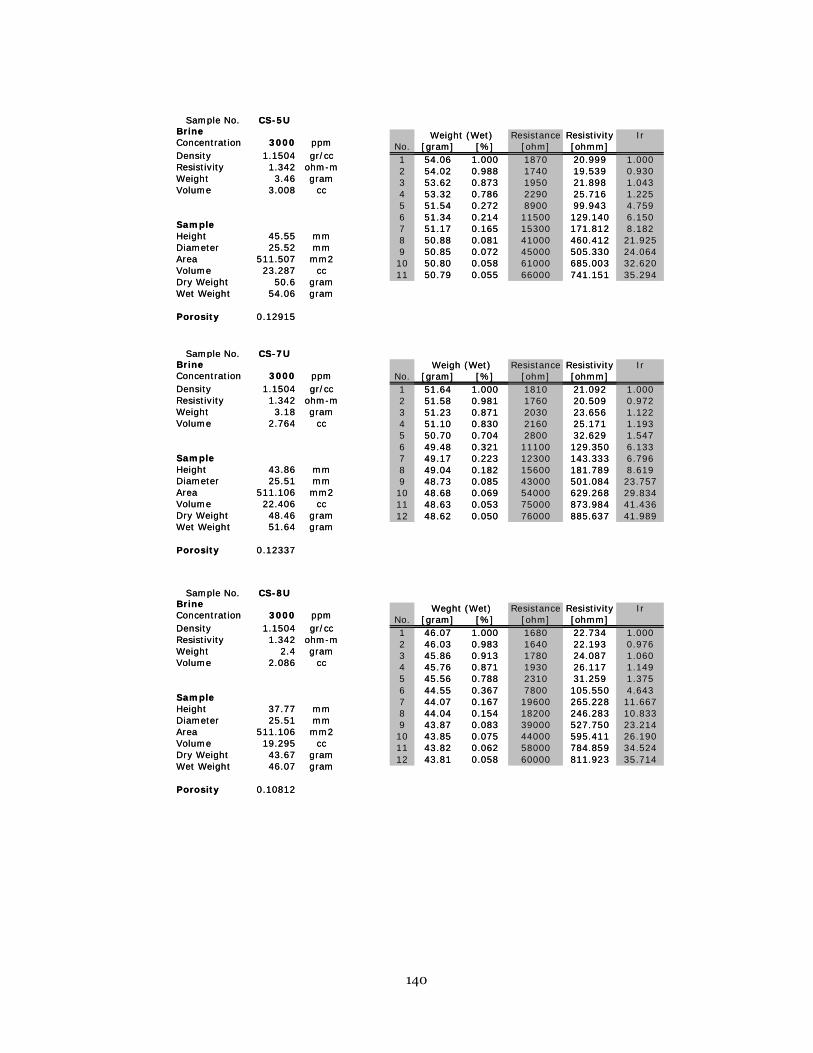
140

Sample No. CS-5UBrine Concentration 3000 ppmDensity 1.1504 gr/ccResistivity 1.342 ohm-mWeight 3.46 gramVolume 3.008 cc

SampleHeight 45.55 mmDiameter 25.52 mmArea 511.507 mm2Volume 23.287 ccDry Weight 50.6 gramWet Weight 54.06 gram

Porosity 0.12915

Resistance Resistivity IrNo. [gram] [%] [ohm] [ohmm]1 54.06 1.000 1870 20.999 1.0002 54.02 0.988 1740 19.539 0.9303 53.62 0.873 1950 21.898 1.0434 53.32 0.786 2290 25.716 1.2255 51.54 0.272 8900 99.943 4.7596 51.34 0.214 11500 129.140 6.1507 51.17 0.165 15300 171.812 8.1828 50.88 0.081 41000 460.412 21.9259 50.85 0.072 45000 505.330 24.06410 50.80 0.058 61000 685.003 32.62011 50.79 0.055 66000 741.151 35.294

Weight (Wet)

Sample No. CS-5UBrine Concentration 3000 ppmDensity 1.1504 gr/ccResistivity 1.342 ohm-mWeight 3.46 gramVolume 3.008 cc

SampleHeight 45.55 mmDiameter 25.52 mmArea 511.507 mm2Volume 23.287 ccDry Weight 50.6 gramWet Weight 54.06 gram

Porosity 0.12915

Resistance Resistivity IrNo. [gram] [%] [ohm] [ohmm]1 54.06 1.000 1870 20.999 1.0002 54.02 0.988 1740 19.539 0.9303 53.62 0.873 1950 21.898 1.0434 53.32 0.786 2290 25.716 1.2255 51.54 0.272 8900 99.943 4.7596 51.34 0.214 11500 129.140 6.1507 51.17 0.165 15300 171.812 8.1828 50.88 0.081 41000 460.412 21.9259 50.85 0.072 45000 505.330 24.06410 50.80 0.058 61000 685.003 32.62011 50.79 0.055 66000 741.151 35.294

Weight (Wet)

Sample No. CS-7UBrine Concentration 3000 ppmDensity 1.1504 gr/ccResistivity 1.342 ohm-mWeight 3.18 gramVolume 2.764 cc

SampleHeight 43.86 mmDiameter 25.51 mmArea 511.106 mm2Volume 22.406 ccDry Weight 48.46 gramWet Weight 51.64 gram

Porosity 0.12337

Resistance Resistivity IrNo. [gram] [%] [ohm] [ohmm]1 51.64 1.000 1810 21.092 1.0002 51.58 0.981 1760 20.509 0.9723 51.23 0.871 2030 23.656 1.1224 51.10 0.830 2160 25.171 1.1935 50.70 0.704 2800 32.629 1.5476 49.48 0.321 11100 129.350 6.1337 49.17 0.223 12300 143.333 6.7968 49.04 0.182 15600 181.789 8.6199 48.73 0.085 43000 501.084 23.75710 48.68 0.069 54000 629.268 29.83411 48.63 0.053 75000 873.984 41.43612 48.62 0.050 76000 885.637 41.989

Weigh (Wet)Sample No. CS-7U

Brine Concentration 3000 ppmDensity 1.1504 gr/ccResistivity 1.342 ohm-mWeight 3.18 gramVolume 2.764 cc

SampleHeight 43.86 mmDiameter 25.51 mmArea 511.106 mm2Volume 22.406 ccDry Weight 48.46 gramWet Weight 51.64 gram

Porosity 0.12337

Resistance Resistivity IrNo. [gram] [%] [ohm] [ohmm]1 51.64 1.000 1810 21.092 1.0002 51.58 0.981 1760 20.509 0.9723 51.23 0.871 2030 23.656 1.1224 51.10 0.830 2160 25.171 1.1935 50.70 0.704 2800 32.629 1.5476 49.48 0.321 11100 129.350 6.1337 49.17 0.223 12300 143.333 6.7968 49.04 0.182 15600 181.789 8.6199 48.73 0.085 43000 501.084 23.75710 48.68 0.069 54000 629.268 29.83411 48.63 0.053 75000 873.984 41.43612 48.62 0.050 76000 885.637 41.989

Weigh (Wet)

Sample No. CS-8UBrine Concentration 3000 ppmDensity 1.1504 gr/ccResistivity 1.342 ohm-mWeight 2.4 gramVolume 2.086 cc

SampleHeight 37.77 mmDiameter 25.51 mmArea 511.106 mm2Volume 19.295 ccDry Weight 43.67 gramWet Weight 46.07 gram

Porosity 0.10812

Resistance Resistivity IrNo. [gram] [%] [ohm] [ohmm]1 46.07 1.000 1680 22.734 1.0002 46.03 0.983 1640 22.193 0.9763 45.86 0.913 1780 24.087 1.0604 45.76 0.871 1930 26.117 1.1495 45.56 0.788 2310 31.259 1.3756 44.55 0.367 7800 105.550 4.6437 44.07 0.167 19600 265.228 11.6678 44.04 0.154 18200 246.283 10.8339 43.87 0.083 39000 527.750 23.21410 43.85 0.075 44000 595.411 26.19011 43.82 0.062 58000 784.859 34.52412 43.81 0.058 60000 811.923 35.714

Weght (Wet)

Sample No. CS-8UBrine Concentration 3000 ppmDensity 1.1504 gr/ccResistivity 1.342 ohm-mWeight 2.4 gramVolume 2.086 cc

SampleHeight 37.77 mmDiameter 25.51 mmArea 511.106 mm2Volume 19.295 ccDry Weight 43.67 gramWet Weight 46.07 gram

Porosity 0.10812

Resistance Resistivity IrNo. [gram] [%] [ohm] [ohmm]1 46.07 1.000 1680 22.734 1.0002 46.03 0.983 1640 22.193 0.9763 45.86 0.913 1780 24.087 1.0604 45.76 0.871 1930 26.117 1.1495 45.56 0.788 2310 31.259 1.3756 44.55 0.367 7800 105.550 4.6437 44.07 0.167 19600 265.228 11.6678 44.04 0.154 18200 246.283 10.8339 43.87 0.083 39000 527.750 23.21410 43.85 0.075 44000 595.411 26.19011 43.82 0.062 58000 784.859 34.52412 43.81 0.058 60000 811.923 35.714

Weght (Wet)

141

B. 10,000 ppm NaCl salinity

Sample No. CS-9UBrine Concentration 3000 ppmDensity 1.1504 gr/ccResistivity 1.342 ohm-mWeight 2.9 gramVolume 2.521 cc

SampleHeight 41.64 mmDiameter 25.53 mmArea 511.908 mm2Volume 21.305 ccDry Weight 46.78 gramWet Weight 49.68 gram

Porosity 0.11832

Resistance Resistivity IrNo. [gram] [%] [ohm] [ohmm]1 49.68 1.000 1670 20.530 1.0002 49.61 0.976 1630 20.039 0.9763 49.26 0.855 1870 22.989 1.1204 49.14 0.814 2010 24.710 1.2045 48.89 0.728 2440 29.997 1.4616 48.20 0.490 5300 65.156 3.1747 47.65 0.300 8500 104.496 5.0908 47.45 0.231 12800 157.359 7.6659 47.04 0.090 35000 430.278 20.95810 47.02 0.083 38000 467.159 22.75411 46.97 0.066 53000 651.563 31.73712 46.96 0.062 55000 676.151 32.934

Weight (Wet)

Sample No. CS-9UBrine Concentration 3000 ppmDensity 1.1504 gr/ccResistivity 1.342 ohm-mWeight 2.9 gramVolume 2.521 cc

SampleHeight 41.64 mmDiameter 25.53 mmArea 511.908 mm2Volume 21.305 ccDry Weight 46.78 gramWet Weight 49.68 gram

Porosity 0.11832

Resistance Resistivity IrNo. [gram] [%] [ohm] [ohmm]1 49.68 1.000 1670 20.530 1.0002 49.61 0.976 1630 20.039 0.9763 49.26 0.855 1870 22.989 1.1204 49.14 0.814 2010 24.710 1.2045 48.89 0.728 2440 29.997 1.4616 48.20 0.490 5300 65.156 3.1747 47.65 0.300 8500 104.496 5.0908 47.45 0.231 12800 157.359 7.6659 47.04 0.090 35000 430.278 20.95810 47.02 0.083 38000 467.159 22.75411 46.97 0.066 53000 651.563 31.73712 46.96 0.062 55000 676.151 32.934

Weight (Wet)

Resistance Resistivity Ir[gram] [%] [ohm]

1 50.71 1.000 750 8.758 1.0002 50.51 0.948 810 9.458 1.0803 50.35 0.907 920 10.743 1.2274 50.23 0.876 920 10.743 1.2275 49.71 0.742 1020 11.910 1.3606 49.59 0.711 1290 15.063 1.7207 49.43 0.670 1250 14.596 1.6678 49.18 0.606 1360 15.880 1.8139 49.09 0.582 1430 16.698 1.90710 48.91 0.536 1670 19.500 2.22711 48.69 0.479 1870 21.835 2.49312 48.49 0.428 2100 24.521 2.80013 48.18 0.348 2520 29.425 3.36014 47.97 0.294 2670 31.177 3.56015 47.65 0.211 3280 38.300 4.37316 47.53 0.180 3800 44.372 5.067

Weight (Wet)No.

Sample No. CS-1LBrine Concentration 10000 ppmDensity 1.1556 gr/ccResistivity 0.5244 ohm-mWeight 3.88 gramVolume 3.358 cc

SampleHeight 43.84 mmDiameter 25.53 mmArea 511.908 mm2Volume 22.431 ccDry Weight 46.83 gramWet Weight 50.71 gram

Porosity 0.14969

Resistance Resistivity Ir[gram] [%] [ohm]

1 50.71 1.000 750 8.758 1.0002 50.51 0.948 810 9.458 1.0803 50.35 0.907 920 10.743 1.2274 50.23 0.876 920 10.743 1.2275 49.71 0.742 1020 11.910 1.3606 49.59 0.711 1290 15.063 1.7207 49.43 0.670 1250 14.596 1.6678 49.18 0.606 1360 15.880 1.8139 49.09 0.582 1430 16.698 1.90710 48.91 0.536 1670 19.500 2.22711 48.69 0.479 1870 21.835 2.49312 48.49 0.428 2100 24.521 2.80013 48.18 0.348 2520 29.425 3.36014 47.97 0.294 2670 31.177 3.56015 47.65 0.211 3280 38.300 4.37316 47.53 0.180 3800 44.372 5.067

Weight (Wet)No.

Sample No. CS-1LBrine Concentration 10000 ppmDensity 1.1556 gr/ccResistivity 0.5244 ohm-mWeight 3.88 gramVolume 3.358 cc

SampleHeight 43.84 mmDiameter 25.53 mmArea 511.908 mm2Volume 22.431 ccDry Weight 46.83 gramWet Weight 50.71 gram

Porosity 0.14969

Resistance Resistivity Ir[gram] [%] [ohm]

1 45.37 1.000 680 8.974 1.0002 45.22 0.957 710 9.370 1.0443 45.08 0.916 760 10.030 1.1184 45.02 0.899 770 10.162 1.1325 44.74 0.818 860 11.350 1.2656 44.65 0.793 920 12.141 1.3537 44.46 0.738 960 12.669 1.4128 44.17 0.654 1110 14.649 1.6329 44.11 0.637 1150 15.177 1.69110 43.83 0.556 1380 18.212 2.02911 43.47 0.452 1800 23.755 2.64712 43.21 0.378 2100 27.714 3.08813 42.95 0.303 2400 31.673 3.52914 42.82 0.265 2500 32.993 3.67615 42.62 0.207 2870 37.876 4.22116 42.45 0.159 3800 50.149 5.588

Weight (Wet)No.

Sample No. CS-2LBrine Concentration 10000 ppmDensity 1.1556 gr/ccResistivity 0.5244 ohm-mWeight 3.47 gramVolume 3.003 cc

SampleHeight 38.85 mmDiameter 25.55 mmArea 512.710 mm2Volume 19.909 ccDry Weight 41.9 gramWet Weight 45.37 gram

Porosity 0.15083

Resistance Resistivity Ir[gram] [%] [ohm]

1 45.37 1.000 680 8.974 1.0002 45.22 0.957 710 9.370 1.0443 45.08 0.916 760 10.030 1.1184 45.02 0.899 770 10.162 1.1325 44.74 0.818 860 11.350 1.2656 44.65 0.793 920 12.141 1.3537 44.46 0.738 960 12.669 1.4128 44.17 0.654 1110 14.649 1.6329 44.11 0.637 1150 15.177 1.69110 43.83 0.556 1380 18.212 2.02911 43.47 0.452 1800 23.755 2.64712 43.21 0.378 2100 27.714 3.08813 42.95 0.303 2400 31.673 3.52914 42.82 0.265 2500 32.993 3.67615 42.62 0.207 2870 37.876 4.22116 42.45 0.159 3800 50.149 5.588

Weight (Wet)No.

Sample No. CS-2LBrine Concentration 10000 ppmDensity 1.1556 gr/ccResistivity 0.5244 ohm-mWeight 3.47 gramVolume 3.003 cc

SampleHeight 38.85 mmDiameter 25.55 mmArea 512.710 mm2Volume 19.909 ccDry Weight 41.9 gramWet Weight 45.37 gram

Porosity 0.15083

142

Resistance Resistivity Ir[gram] [%] [ohm]

1 51.15 1.000 840 9.794 1.0002 51.02 0.966 870 10.144 1.0363 50.78 0.903 1010 11.776 1.2024 50.65 0.869 1040 12.126 1.2385 50.27 0.770 1100 12.826 1.3106 50.16 0.741 1200 13.992 1.4297 50.09 0.723 1250 14.574 1.4888 49.89 0.670 1280 14.924 1.5249 49.81 0.649 1320 15.391 1.57110 49.61 0.597 1550 18.072 1.84511 49.38 0.537 1780 20.754 2.11912 48.80 0.385 2540 29.615 3.02413 48.41 0.283 3010 35.095 3.58314 48.31 0.257 3150 36.728 3.75015 48.01 0.178 4100 47.804 4.88116 47.77 0.115 6100 71.124 7.262

Weight (Wet)No.

Sample No. CS-3LBrine Concentration 10000 ppmDensity 1.1556 gr/ccResistivity 0.5244 ohm-mWeight 3.82 gramVolume 3.306 cc

SampleHeight 43.87 mmDiameter 25.52 mmArea 511.507 mm2Volume 22.428 ccDry Weight 47.33 gramWet Weight 51.15 gram

Porosity 0.14739

Resistance Resistivity Ir[gram] [%] [ohm]

1 51.15 1.000 840 9.794 1.0002 51.02 0.966 870 10.144 1.0363 50.78 0.903 1010 11.776 1.2024 50.65 0.869 1040 12.126 1.2385 50.27 0.770 1100 12.826 1.3106 50.16 0.741 1200 13.992 1.4297 50.09 0.723 1250 14.574 1.4888 49.89 0.670 1280 14.924 1.5249 49.81 0.649 1320 15.391 1.57110 49.61 0.597 1550 18.072 1.84511 49.38 0.537 1780 20.754 2.11912 48.80 0.385 2540 29.615 3.02413 48.41 0.283 3010 35.095 3.58314 48.31 0.257 3150 36.728 3.75015 48.01 0.178 4100 47.804 4.88116 47.77 0.115 6100 71.124 7.262

Weight (Wet)No.

Sample No. CS-3LBrine Concentration 10000 ppmDensity 1.1556 gr/ccResistivity 0.5244 ohm-mWeight 3.82 gramVolume 3.306 cc

SampleHeight 43.87 mmDiameter 25.52 mmArea 511.507 mm2Volume 22.428 ccDry Weight 47.33 gramWet Weight 51.15 gram

Porosity 0.14739

Resistance Resistivity Ir[gram] [%] [ohm]

1 52.02 1.000 840 9.552 1.0002 51.86 0.959 880 10.007 1.0483 51.75 0.931 910 10.348 1.0834 51.64 0.903 960 10.917 1.1435 51.38 0.837 980 11.144 1.1676 51.25 0.804 1200 13.646 1.4297 51.14 0.776 1180 13.419 1.4058 50.95 0.727 1180 13.419 1.4059 50.82 0.694 1240 14.101 1.47610 50.59 0.635 1450 16.489 1.72611 50.19 0.533 1790 20.356 2.13112 49.56 0.372 2680 30.477 3.19013 49.16 0.270 3190 36.276 3.79814 48.97 0.222 3500 39.802 4.16715 48.53 0.110 6500 73.917 7.73816 48.39 0.074 9700 110.307 11.548

Weight (Wet)No.

Sample No. CS-4LBrine Concentration 10000 ppmDensity 1.1556 gr/ccResistivity 0.5244 ohm-mWeight 3.92 gramVolume 3.392 cc

SampleHeight 44.98 mmDiameter 25.52 mmArea 511.507 mm2Volume 22.996 ccDry Weight 48.1 gramWet Weight 52.02 gram

Porosity 0.14751

Resistance Resistivity Ir[gram] [%] [ohm]

1 52.02 1.000 840 9.552 1.0002 51.86 0.959 880 10.007 1.0483 51.75 0.931 910 10.348 1.0834 51.64 0.903 960 10.917 1.1435 51.38 0.837 980 11.144 1.1676 51.25 0.804 1200 13.646 1.4297 51.14 0.776 1180 13.419 1.4058 50.95 0.727 1180 13.419 1.4059 50.82 0.694 1240 14.101 1.47610 50.59 0.635 1450 16.489 1.72611 50.19 0.533 1790 20.356 2.13112 49.56 0.372 2680 30.477 3.19013 49.16 0.270 3190 36.276 3.79814 48.97 0.222 3500 39.802 4.16715 48.53 0.110 6500 73.917 7.73816 48.39 0.074 9700 110.307 11.548

Weight (Wet)No.

Sample No. CS-4LBrine Concentration 10000 ppmDensity 1.1556 gr/ccResistivity 0.5244 ohm-mWeight 3.92 gramVolume 3.392 cc

SampleHeight 44.98 mmDiameter 25.52 mmArea 511.507 mm2Volume 22.996 ccDry Weight 48.1 gramWet Weight 52.02 gram

Porosity 0.14751

Sample No. CS-5LBrine Concentration 10000 ppmDensity 1.1556 gr/ccResistivity 0.5244 ohm-mWeight 3.77 gramVolume 3.262 cc

SampleHeight 43.87 mmDiameter 25.54 mmArea 512.309 mm2Volume 22.464 ccDry Weight 47.47 gramWet Weight 51.24 gram

Porosity 0.14523

Resistance Resistivity Ir[gram] [%] [ohm]

1 51.24 1.000 820 9.576 1.0002 51.10 0.963 850 9.926 1.0373 50.86 0.899 920 10.744 1.1224 50.79 0.881 950 11.094 1.1595 50.36 0.767 1090 12.729 1.3296 50.24 0.735 1210 14.130 1.4767 50.13 0.706 1250 14.597 1.5248 49.88 0.639 1340 15.648 1.6349 49.84 0.629 1380 16.115 1.68310 49.67 0.584 1530 17.867 1.86611 49.44 0.523 1820 21.254 2.22012 49.08 0.427 2270 26.509 2.76813 48.67 0.318 2750 32.114 3.35414 48.43 0.255 3280 38.303 4.00015 48.28 0.215 3500 40.873 4.26816 48.12 0.172 4300 50.215 5.244

Weight (Wet)No.

Sample No. CS-5LBrine Concentration 10000 ppmDensity 1.1556 gr/ccResistivity 0.5244 ohm-mWeight 3.77 gramVolume 3.262 cc

SampleHeight 43.87 mmDiameter 25.54 mmArea 512.309 mm2Volume 22.464 ccDry Weight 47.47 gramWet Weight 51.24 gram

Porosity 0.14523

Resistance Resistivity Ir[gram] [%] [ohm]

1 51.24 1.000 820 9.576 1.0002 51.10 0.963 850 9.926 1.0373 50.86 0.899 920 10.744 1.1224 50.79 0.881 950 11.094 1.1595 50.36 0.767 1090 12.729 1.3296 50.24 0.735 1210 14.130 1.4767 50.13 0.706 1250 14.597 1.5248 49.88 0.639 1340 15.648 1.6349 49.84 0.629 1380 16.115 1.68310 49.67 0.584 1530 17.867 1.86611 49.44 0.523 1820 21.254 2.22012 49.08 0.427 2270 26.509 2.76813 48.67 0.318 2750 32.114 3.35414 48.43 0.255 3280 38.303 4.00015 48.28 0.215 3500 40.873 4.26816 48.12 0.172 4300 50.215 5.244

Weight (Wet)No.

143

Sample No. CS-7LBrine Concentration 10000 ppmDensity 1.1556 gr/ccResistivity 0.5244 ohm-mWeight 3.47 gramVolume 3.003 cc

SampleHeight 38.87 mmDiameter 25.53 mmArea 511.908 mm2Volume 19.888 ccDry Weight 41.96 gramWet Weight 45.43 gram

Porosity 0.15099

Resistance Resistivity Ir[gram] [%] [ohm]

1 45.43 1.000 710 9.351 1.0002 45.29 0.960 750 9.877 1.0563 45.20 0.934 780 10.272 1.0994 45.10 0.905 820 10.799 1.1555 44.78 0.813 860 11.326 1.2116 44.70 0.790 940 12.380 1.3247 44.61 0.764 930 12.248 1.3108 44.30 0.674 1180 15.540 1.6629 44.20 0.646 1140 15.013 1.60610 44.06 0.605 1270 16.726 1.78911 43.79 0.527 1480 19.491 2.08512 43.57 0.464 1710 22.520 2.40813 43.27 0.378 1940 25.549 2.73214 42.92 0.277 2350 30.949 3.31015 42.52 0.161 3700 48.728 5.21116 42.51 0.159 4100 53.996 5.775

Weigh (Wet)No.Sample No. CS-7L

Brine Concentration 10000 ppmDensity 1.1556 gr/ccResistivity 0.5244 ohm-mWeight 3.47 gramVolume 3.003 cc

SampleHeight 38.87 mmDiameter 25.53 mmArea 511.908 mm2Volume 19.888 ccDry Weight 41.96 gramWet Weight 45.43 gram

Porosity 0.15099

Resistance Resistivity Ir[gram] [%] [ohm]

1 45.43 1.000 710 9.351 1.0002 45.29 0.960 750 9.877 1.0563 45.20 0.934 780 10.272 1.0994 45.10 0.905 820 10.799 1.1555 44.78 0.813 860 11.326 1.2116 44.70 0.790 940 12.380 1.3247 44.61 0.764 930 12.248 1.3108 44.30 0.674 1180 15.540 1.6629 44.20 0.646 1140 15.013 1.60610 44.06 0.605 1270 16.726 1.78911 43.79 0.527 1480 19.491 2.08512 43.57 0.464 1710 22.520 2.40813 43.27 0.378 1940 25.549 2.73214 42.92 0.277 2350 30.949 3.31015 42.52 0.161 3700 48.728 5.21116 42.51 0.159 4100 53.996 5.775

Weigh (Wet)No.

Sample No. CS-8LBrine Concentration 10000 ppmDensity 1.1556 gr/ccResistivity 0.5244 ohm-mWeight 3.3 gramVolume 2.856 cc

SampleHeight 38.29 mmDiameter 25.55 mmArea 512.710 mm2Volume 19.622 ccDry Weight 41.2 gramWet Weight 44.5 gram

Porosity 0.14554

Resistance Resistivity Ir[gram] [%] [ohm] [ohmm]

1 44.50 1.000 690 9.239 1.0002 44.36 0.958 720 9.641 1.0433 44.17 0.900 810 10.846 1.1744 44.08 0.873 840 11.248 1.2175 43.86 0.806 880 11.783 1.2756 43.78 0.782 950 12.721 1.3777 43.66 0.745 1020 13.658 1.4788 43.41 0.670 1150 15.399 1.6679 43.30 0.636 1220 16.336 1.76810 43.01 0.548 1510 20.219 2.18811 42.87 0.506 1640 21.960 2.37712 42.50 0.394 2300 30.797 3.33313 42.23 0.312 2420 32.404 3.50714 42.02 0.248 2810 37.626 4.07215 41.72 0.158 3500 46.866 5.07216 41.61 0.124 4900 65.612 7.101

Weght (Wet)No.Sample No. CS-8L

Brine Concentration 10000 ppmDensity 1.1556 gr/ccResistivity 0.5244 ohm-mWeight 3.3 gramVolume 2.856 cc

SampleHeight 38.29 mmDiameter 25.55 mmArea 512.710 mm2Volume 19.622 ccDry Weight 41.2 gramWet Weight 44.5 gram

Porosity 0.14554

Resistance Resistivity Ir[gram] [%] [ohm] [ohmm]

1 44.50 1.000 690 9.239 1.0002 44.36 0.958 720 9.641 1.0433 44.17 0.900 810 10.846 1.1744 44.08 0.873 840 11.248 1.2175 43.86 0.806 880 11.783 1.2756 43.78 0.782 950 12.721 1.3777 43.66 0.745 1020 13.658 1.4788 43.41 0.670 1150 15.399 1.6679 43.30 0.636 1220 16.336 1.76810 43.01 0.548 1510 20.219 2.18811 42.87 0.506 1640 21.960 2.37712 42.50 0.394 2300 30.797 3.33313 42.23 0.312 2420 32.404 3.50714 42.02 0.248 2810 37.626 4.07215 41.72 0.158 3500 46.866 5.07216 41.61 0.124 4900 65.612 7.101

Weght (Wet)No.

Sample No. CS-9LBrine Concentration 10000 ppmDensity 1.1556 gr/ccResistivity 0.5244 ohm-mWeight 3.52 gramVolume 3.046 cc

SampleHeight 42.18 mmDiameter 25.55 mmArea 512.710 mm2Volume 21.615 ccDry Weight 44.85 gramWet Weight 48.37 gram

Porosity 0.14092

Resistance Resistivity Ir[gram] [%] [ohm] [ohmm]

1 48.37 1.000 810 9.846 1.0002 48.27 0.972 820 9.967 1.0123 48.11 0.926 870 10.575 1.0744 48.03 0.903 1170 14.222 1.4445 47.59 0.778 1050 12.763 1.2966 47.50 0.753 1170 14.222 1.4447 47.39 0.722 1170 14.222 1.4448 47.10 0.639 1310 15.923 1.6179 47.03 0.619 1380 16.774 1.70410 46.77 0.545 1700 20.664 2.09911 46.43 0.449 2070 25.161 2.55612 46.02 0.332 2700 32.819 3.33313 45.94 0.310 2620 31.847 3.23514 45.80 0.270 2800 34.035 3.45715 45.39 0.153 4400 53.483 5.43216 45.23 0.108 6300 76.578 7.778

Weight (Wet)No.Sample No. CS-9L

Brine Concentration 10000 ppmDensity 1.1556 gr/ccResistivity 0.5244 ohm-mWeight 3.52 gramVolume 3.046 cc

SampleHeight 42.18 mmDiameter 25.55 mmArea 512.710 mm2Volume 21.615 ccDry Weight 44.85 gramWet Weight 48.37 gram

Porosity 0.14092

Resistance Resistivity Ir[gram] [%] [ohm] [ohmm]

1 48.37 1.000 810 9.846 1.0002 48.27 0.972 820 9.967 1.0123 48.11 0.926 870 10.575 1.0744 48.03 0.903 1170 14.222 1.4445 47.59 0.778 1050 12.763 1.2966 47.50 0.753 1170 14.222 1.4447 47.39 0.722 1170 14.222 1.4448 47.10 0.639 1310 15.923 1.6179 47.03 0.619 1380 16.774 1.70410 46.77 0.545 1700 20.664 2.09911 46.43 0.449 2070 25.161 2.55612 46.02 0.332 2700 32.819 3.33313 45.94 0.310 2620 31.847 3.23514 45.80 0.270 2800 34.035 3.45715 45.39 0.153 4400 53.483 5.43216 45.23 0.108 6300 76.578 7.778

Weight (Wet)No.

144

Sample No. CS-1UBrine Concentration 10000 ppmDensity 1.1556 gr/ccResistivity 0.5244 ohm-mWeight 3.16 gramVolume 2.735 cc

SampleHeight 42.75 mmDiameter 25.51 mmArea 511.106 mm2Volume 21.839 ccDry Weight 46.64 gramWet Weight 49.8 gram

Porosity 0.12521

Resistance Resistivity IrNo. [gram] [%] [ohm] [ohmm]1 49.80 1.000 1160 13.869 1.0002 49.72 0.975 1200 14.347 1.0343 49.55 0.921 1310 15.662 1.1294 49.46 0.892 1360 16.260 1.1725 49.18 0.804 1530 18.292 1.3196 49.10 0.778 1670 19.966 1.4407 48.96 0.734 1760 21.042 1.5178 48.68 0.646 2100 25.107 1.8109 48.54 0.601 2390 28.574 2.06010 48.15 0.478 3800 45.432 3.27611 47.70 0.335 5500 65.756 4.74112 47.16 0.165 11200 133.904 9.65513 46.91 0.085 22100 264.221 19.05214 46.89 0.079 22800 272.590 19.65515 46.81 0.054 30300 362.257 26.12116 46.77 0.041 37000 442.361 31.897

Weight (Wet)Sample No. CS-1U

Brine Concentration 10000 ppmDensity 1.1556 gr/ccResistivity 0.5244 ohm-mWeight 3.16 gramVolume 2.735 cc

SampleHeight 42.75 mmDiameter 25.51 mmArea 511.106 mm2Volume 21.839 ccDry Weight 46.64 gramWet Weight 49.8 gram

Porosity 0.12521

Resistance Resistivity IrNo. [gram] [%] [ohm] [ohmm]1 49.80 1.000 1160 13.869 1.0002 49.72 0.975 1200 14.347 1.0343 49.55 0.921 1310 15.662 1.1294 49.46 0.892 1360 16.260 1.1725 49.18 0.804 1530 18.292 1.3196 49.10 0.778 1670 19.966 1.4407 48.96 0.734 1760 21.042 1.5178 48.68 0.646 2100 25.107 1.8109 48.54 0.601 2390 28.574 2.06010 48.15 0.478 3800 45.432 3.27611 47.70 0.335 5500 65.756 4.74112 47.16 0.165 11200 133.904 9.65513 46.91 0.085 22100 264.221 19.05214 46.89 0.079 22800 272.590 19.65515 46.81 0.054 30300 362.257 26.12116 46.77 0.041 37000 442.361 31.897

Weight (Wet)

Sample No. CS-2UBrine Concentration 10000 ppmDensity 1.1556 gr/ccResistivity 0.5244 ohm-mWeight 3.4 gramVolume 2.942 cc

SampleHeight 44.98 mmDiameter 25.51 mmArea 511.106 mm2Volume 22.978 ccDry Weight 49.63 gramWet Weight 53.03 gram

Porosity 0.12804

Resistance Resistivity IrNo. [gram] [%] [ohm] [ohmm]1 53.03 1.000 1230 13.976 1.0002 52.92 0.968 1260 14.317 1.0243 52.74 0.915 1380 15.681 1.1224 52.63 0.882 1460 16.590 1.1875 51.85 0.653 2200 24.999 1.7896 51.71 0.612 2560 29.089 2.0817 51.49 0.547 3080 34.998 2.5048 50.93 0.382 5400 61.360 4.3909 50.88 0.368 5400 61.360 4.39010 50.71 0.318 6200 70.450 5.04111 50.54 0.268 6800 77.268 5.52812 50.23 0.176 11200 127.265 9.10613 49.97 0.100 21400 243.167 17.39814 49.93 0.088 23000 261.348 18.69915 49.83 0.059 30600 347.706 24.87816 49.77 0.041 42000 477.244 34.146

Weight (Wet)Sample No. CS-2U

Brine Concentration 10000 ppmDensity 1.1556 gr/ccResistivity 0.5244 ohm-mWeight 3.4 gramVolume 2.942 cc

SampleHeight 44.98 mmDiameter 25.51 mmArea 511.106 mm2Volume 22.978 ccDry Weight 49.63 gramWet Weight 53.03 gram

Porosity 0.12804

Resistance Resistivity IrNo. [gram] [%] [ohm] [ohmm]1 53.03 1.000 1230 13.976 1.0002 52.92 0.968 1260 14.317 1.0243 52.74 0.915 1380 15.681 1.1224 52.63 0.882 1460 16.590 1.1875 51.85 0.653 2200 24.999 1.7896 51.71 0.612 2560 29.089 2.0817 51.49 0.547 3080 34.998 2.5048 50.93 0.382 5400 61.360 4.3909 50.88 0.368 5400 61.360 4.39010 50.71 0.318 6200 70.450 5.04111 50.54 0.268 6800 77.268 5.52812 50.23 0.176 11200 127.265 9.10613 49.97 0.100 21400 243.167 17.39814 49.93 0.088 23000 261.348 18.69915 49.83 0.059 30600 347.706 24.87816 49.77 0.041 42000 477.244 34.146

Weight (Wet)

Sample No. CS-3UBrine Concentration 10000 ppmDensity 1.1556 gr/ccResistivity 0.5244 ohm-mWeight 3.39 gramVolume 2.93354 cc

SampleHeight 45.56 mmDiameter 25.52 mmArea 511.507 mm2Volume 23.292 ccDry Weight 50.59 gramWet Weight 53.98 gram

Porosity 0.12594

Resistance Resistivity IrNo. [gram] [%] [ohm] [ohmm]1 53.98 1.000 1290 14.483 1.0002 53.84 0.959 1340 15.044 1.0393 53.65 0.903 1440 16.167 1.1164 53.54 0.870 1510 16.953 1.1715 52.85 0.667 2240 25.149 1.7366 52.76 0.640 2540 28.517 1.9697 52.68 0.617 2590 29.078 2.0088 52.39 0.531 3500 39.295 2.7139 52.30 0.504 3800 42.663 2.94610 52.03 0.425 4700 52.767 3.64311 51.68 0.322 5700 63.994 4.41912 51.16 0.168 10600 119.007 8.21713 50.95 0.106 16500 185.247 12.79114 50.88 0.086 20200 226.787 15.65915 50.78 0.056 23900 268.328 18.52716 50.67 0.024 44000 493.992 34.109

Weight (Wet)Sample No. CS-3U

Brine Concentration 10000 ppmDensity 1.1556 gr/ccResistivity 0.5244 ohm-mWeight 3.39 gramVolume 2.93354 cc

SampleHeight 45.56 mmDiameter 25.52 mmArea 511.507 mm2Volume 23.292 ccDry Weight 50.59 gramWet Weight 53.98 gram

Porosity 0.12594

Resistance Resistivity IrNo. [gram] [%] [ohm] [ohmm]1 53.98 1.000 1290 14.483 1.0002 53.84 0.959 1340 15.044 1.0393 53.65 0.903 1440 16.167 1.1164 53.54 0.870 1510 16.953 1.1715 52.85 0.667 2240 25.149 1.7366 52.76 0.640 2540 28.517 1.9697 52.68 0.617 2590 29.078 2.0088 52.39 0.531 3500 39.295 2.7139 52.30 0.504 3800 42.663 2.94610 52.03 0.425 4700 52.767 3.64311 51.68 0.322 5700 63.994 4.41912 51.16 0.168 10600 119.007 8.21713 50.95 0.106 16500 185.247 12.79114 50.88 0.086 20200 226.787 15.65915 50.78 0.056 23900 268.328 18.52716 50.67 0.024 44000 493.992 34.109

Weight (Wet)

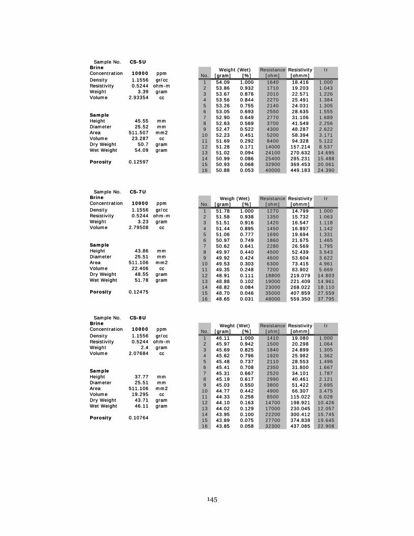
145

Sample No. CS-5UBrine Concentration 10000 ppmDensity 1.1556 gr/ccResistivity 0.5244 ohm-mWeight 3.39 gramVolume 2.93354 cc

SampleHeight 45.55 mmDiameter 25.52 mmArea 511.507 mm2Volume 23.287 ccDry Weight 50.7 gramWet Weight 54.09 gram

Porosity 0.12597

Resistance Resistivity IrNo. [gram] [%] [ohm] [ohmm]1 54.09 1.000 1640 18.416 1.0002 53.86 0.932 1710 19.203 1.0433 53.67 0.876 2010 22.571 1.2264 53.56 0.844 2270 25.491 1.3845 53.26 0.755 2140 24.031 1.3056 53.05 0.693 2550 28.635 1.5557 52.90 0.649 2770 31.106 1.6898 52.63 0.569 3700 41.549 2.2569 52.47 0.522 4300 48.287 2.62210 52.23 0.451 5200 58.394 3.17111 51.69 0.292 8400 94.328 5.12212 51.28 0.171 14000 157.214 8.53713 51.02 0.094 24100 270.632 14.69514 50.99 0.086 25400 285.231 15.48815 50.93 0.068 32900 369.453 20.06116 50.88 0.053 40000 449.183 24.390

Weight (Wet)

Sample No. CS-5UBrine Concentration 10000 ppmDensity 1.1556 gr/ccResistivity 0.5244 ohm-mWeight 3.39 gramVolume 2.93354 cc

SampleHeight 45.55 mmDiameter 25.52 mmArea 511.507 mm2Volume 23.287 ccDry Weight 50.7 gramWet Weight 54.09 gram

Porosity 0.12597

Resistance Resistivity IrNo. [gram] [%] [ohm] [ohmm]1 54.09 1.000 1640 18.416 1.0002 53.86 0.932 1710 19.203 1.0433 53.67 0.876 2010 22.571 1.2264 53.56 0.844 2270 25.491 1.3845 53.26 0.755 2140 24.031 1.3056 53.05 0.693 2550 28.635 1.5557 52.90 0.649 2770 31.106 1.6898 52.63 0.569 3700 41.549 2.2569 52.47 0.522 4300 48.287 2.62210 52.23 0.451 5200 58.394 3.17111 51.69 0.292 8400 94.328 5.12212 51.28 0.171 14000 157.214 8.53713 51.02 0.094 24100 270.632 14.69514 50.99 0.086 25400 285.231 15.48815 50.93 0.068 32900 369.453 20.06116 50.88 0.053 40000 449.183 24.390

Weight (Wet)

Sample No. CS-7UBrine Concentration 10000 ppmDensity 1.1556 gr/ccResistivity 0.5244 ohm-mWeight 3.23 gramVolume 2.79508 cc

SampleHeight 43.86 mmDiameter 25.51 mmArea 511.106 mm2Volume 22.406 ccDry Weight 48.55 gramWet Weight 51.78 gram

Porosity 0.12475

Resistance Resistivity IrNo. [gram] [%] [ohm] [ohmm]1 51.78 1.000 1270 14.799 1.0002 51.58 0.938 1350 15.732 1.0633 51.51 0.916 1420 16.547 1.1184 51.44 0.895 1450 16.897 1.1425 51.06 0.777 1690 19.694 1.3316 50.97 0.749 1860 21.675 1.4657 50.62 0.641 2280 26.569 1.7958 49.97 0.440 4500 52.439 3.5439 49.92 0.424 4600 53.604 3.62210 49.53 0.303 6300 73.415 4.96111 49.35 0.248 7200 83.902 5.66912 48.91 0.111 18800 219.079 14.80313 48.88 0.102 19000 221.409 14.96114 48.82 0.084 23000 268.022 18.11015 48.70 0.046 35000 407.859 27.55916 48.65 0.031 48000 559.350 37.795

Weigh (Wet)Sample No. CS-7U

Brine Concentration 10000 ppmDensity 1.1556 gr/ccResistivity 0.5244 ohm-mWeight 3.23 gramVolume 2.79508 cc

SampleHeight 43.86 mmDiameter 25.51 mmArea 511.106 mm2Volume 22.406 ccDry Weight 48.55 gramWet Weight 51.78 gram

Porosity 0.12475

Resistance Resistivity IrNo. [gram] [%] [ohm] [ohmm]1 51.78 1.000 1270 14.799 1.0002 51.58 0.938 1350 15.732 1.0633 51.51 0.916 1420 16.547 1.1184 51.44 0.895 1450 16.897 1.1425 51.06 0.777 1690 19.694 1.3316 50.97 0.749 1860 21.675 1.4657 50.62 0.641 2280 26.569 1.7958 49.97 0.440 4500 52.439 3.5439 49.92 0.424 4600 53.604 3.62210 49.53 0.303 6300 73.415 4.96111 49.35 0.248 7200 83.902 5.66912 48.91 0.111 18800 219.079 14.80313 48.88 0.102 19000 221.409 14.96114 48.82 0.084 23000 268.022 18.11015 48.70 0.046 35000 407.859 27.55916 48.65 0.031 48000 559.350 37.795

Weigh (Wet)

Sample No. CS-8UBrine Concentration 10000 ppmDensity 1.1556 gr/ccResistivity 0.5244 ohm-mWeight 2.4 gramVolume 2.07684 cc

SampleHeight 37.77 mmDiameter 25.51 mmArea 511.106 mm2Volume 19.295 ccDry Weight 43.71 gramWet Weight 46.11 gram

Porosity 0.10764

Resistance Resistivity IrNo. [gram] [%] [ohm] [ohmm]1 46.11 1.000 1410 19.080 1.0002 45.97 0.942 1500 20.298 1.0643 45.69 0.825 1840 24.899 1.3054 45.62 0.796 1920 25.982 1.3625 45.48 0.737 2110 28.553 1.4966 45.41 0.708 2350 31.800 1.6677 45.31 0.667 2520 34.101 1.7878 45.19 0.617 2990 40.461 2.1219 45.03 0.550 3800 51.422 2.69510 44.77 0.442 4900 66.307 3.47511 44.33 0.258 8500 115.022 6.02812 44.10 0.163 14700 198.921 10.42613 44.02 0.129 17000 230.045 12.05714 43.95 0.100 22200 300.412 15.74515 43.89 0.075 27700 374.838 19.64516 43.85 0.058 32300 437.085 22.908

Weght (Wet)

Sample No. CS-8UBrine Concentration 10000 ppmDensity 1.1556 gr/ccResistivity 0.5244 ohm-mWeight 2.4 gramVolume 2.07684 cc

SampleHeight 37.77 mmDiameter 25.51 mmArea 511.106 mm2Volume 19.295 ccDry Weight 43.71 gramWet Weight 46.11 gram

Porosity 0.10764

Resistance Resistivity IrNo. [gram] [%] [ohm] [ohmm]1 46.11 1.000 1410 19.080 1.0002 45.97 0.942 1500 20.298 1.0643 45.69 0.825 1840 24.899 1.3054 45.62 0.796 1920 25.982 1.3625 45.48 0.737 2110 28.553 1.4966 45.41 0.708 2350 31.800 1.6677 45.31 0.667 2520 34.101 1.7878 45.19 0.617 2990 40.461 2.1219 45.03 0.550 3800 51.422 2.69510 44.77 0.442 4900 66.307 3.47511 44.33 0.258 8500 115.022 6.02812 44.10 0.163 14700 198.921 10.42613 44.02 0.129 17000 230.045 12.05714 43.95 0.100 22200 300.412 15.74515 43.89 0.075 27700 374.838 19.64516 43.85 0.058 32300 437.085 22.908

Weght (Wet)

146

C.20,000 ppm NaCl salinity

Sample No. CS-9UBrine Concentration 10000 ppmDensity 1.1556 gr/ccResistivity 0.5244 ohm-mWeight 2.9 gramVolume 2.50952 cc

SampleHeight 41.64 mmDiameter 25.53 mmArea 511.908 mm2Volume 21.305 ccDry Weight 46.87 gramWet Weight 49.77 gram

Porosity 0.11779

Resistance Resistivity IrNo. [gram] [%] [ohm] [ohmm]1 49.77 1.000 1280 15.736 1.0002 49.67 0.966 1300 15.982 1.0163 49.52 0.914 1400 17.211 1.0944 49.44 0.886 1440 17.703 1.1255 49.23 0.814 1560 19.178 1.2196 49.13 0.779 1720 21.145 1.3447 49.02 0.741 1780 21.883 1.3918 48.65 0.614 2470 30.365 1.9309 48.46 0.548 3180 39.094 2.48410 48.09 0.421 4600 56.551 3.59411 47.68 0.279 6400 78.679 5.00012 47.50 0.217 7900 97.120 6.17213 47.26 0.134 13400 164.735 10.46914 47.18 0.107 16800 206.533 13.12515 47.10 0.079 21300 261.855 16.64116 47.06 0.066 24200 297.506 18.906

Weight (Wet)

Sample No. CS-9UBrine Concentration 10000 ppmDensity 1.1556 gr/ccResistivity 0.5244 ohm-mWeight 2.9 gramVolume 2.50952 cc

SampleHeight 41.64 mmDiameter 25.53 mmArea 511.908 mm2Volume 21.305 ccDry Weight 46.87 gramWet Weight 49.77 gram

Porosity 0.11779

Resistance Resistivity IrNo. [gram] [%] [ohm] [ohmm]1 49.77 1.000 1280 15.736 1.0002 49.67 0.966 1300 15.982 1.0163 49.52 0.914 1400 17.211 1.0944 49.44 0.886 1440 17.703 1.1255 49.23 0.814 1560 19.178 1.2196 49.13 0.779 1720 21.145 1.3447 49.02 0.741 1780 21.883 1.3918 48.65 0.614 2470 30.365 1.9309 48.46 0.548 3180 39.094 2.48410 48.09 0.421 4600 56.551 3.59411 47.68 0.279 6400 78.679 5.00012 47.50 0.217 7900 97.120 6.17213 47.26 0.134 13400 164.735 10.46914 47.18 0.107 16800 206.533 13.12515 47.10 0.079 21300 261.855 16.64116 47.06 0.066 24200 297.506 18.906

Weight (Wet)

Sample No. CS-1LBrine Concentration 20000 ppmDensity 1.1636 gr/ccResistivity 0.278 ohm-mWeight 4.13 gramVolume 3.549 cc

SampleHeight 43.84 mmDiameter 25.53 mmArea 511.908 mm2Volume 22.431 ccDry Weight 46.6 gramWet Weight 50.73 gram

Porosity 0.15824

Resistance Resistivity Ir[gram] [%] [ohm] [ohmm]

1 50.73 1.000 360 4.204 1.0002 50.62 0.973 400 4.671 1.1113 50.56 0.959 400 4.671 1.1114 50.49 0.942 410 4.787 1.1395 50.37 0.913 440 5.138 1.2226 50.18 0.867 460 5.371 1.2787 50.05 0.835 490 5.722 1.3618 49.70 0.751 560 6.539 1.5569 49.45 0.690 610 7.123 1.69410 49.29 0.651 680 7.940 1.88911 48.88 0.552 910 10.626 2.52812 48.74 0.518 1000 11.677 2.77813 48.49 0.458 1190 13.895 3.30614 48.31 0.414 1300 15.180 3.61115 47.20 0.145 8100 94.581 22.500

Weight (Wet)No.

Sample No. CS-1LBrine Concentration 20000 ppmDensity 1.1636 gr/ccResistivity 0.278 ohm-mWeight 4.13 gramVolume 3.549 cc

SampleHeight 43.84 mmDiameter 25.53 mmArea 511.908 mm2Volume 22.431 ccDry Weight 46.6 gramWet Weight 50.73 gram

Porosity 0.15824

Resistance Resistivity Ir[gram] [%] [ohm] [ohmm]

1 50.73 1.000 360 4.204 1.0002 50.62 0.973 400 4.671 1.1113 50.56 0.959 400 4.671 1.1114 50.49 0.942 410 4.787 1.1395 50.37 0.913 440 5.138 1.2226 50.18 0.867 460 5.371 1.2787 50.05 0.835 490 5.722 1.3618 49.70 0.751 560 6.539 1.5569 49.45 0.690 610 7.123 1.69410 49.29 0.651 680 7.940 1.88911 48.88 0.552 910 10.626 2.52812 48.74 0.518 1000 11.677 2.77813 48.49 0.458 1190 13.895 3.30614 48.31 0.414 1300 15.180 3.61115 47.20 0.145 8100 94.581 22.500

Weight (Wet)No.

Sample No. CS-2LBrine Concentration 20000 ppmDensity 1.1636 gr/ccResistivity 0.278 ohm-mWeight 3.7 gramVolume 3.180 cc

SampleHeight 38.85 mmDiameter 25.55 mmArea 512.710 mm2Volume 19.909 ccDry Weight 41.71 gramWet Weight 45.41 gram

Porosity 0.15972

Resistance Resistivity Ir[gram] [%] [ohm] [ohmm]

1 45.41 1.000 330 4.355 1.0002 45.31 0.973 360 4.751 1.0913 45.25 0.957 360 4.751 1.0914 45.19 0.941 370 4.883 1.1215 44.93 0.870 430 5.675 1.3036 44.72 0.814 460 6.071 1.3947 44.61 0.784 480 6.335 1.4558 44.49 0.751 500 6.599 1.5159 44.03 0.627 640 8.446 1.93910 43.88 0.586 730 9.634 2.21211 43.79 0.562 780 10.294 2.36412 43.55 0.497 940 12.405 2.84813 43.41 0.459 1060 13.989 3.21214 43.32 0.435 1090 14.385 3.30315 42.99 0.346 1330 17.552 4.030

Weight (Wet)No.

Sample No. CS-2LBrine Concentration 20000 ppmDensity 1.1636 gr/ccResistivity 0.278 ohm-mWeight 3.7 gramVolume 3.180 cc

SampleHeight 38.85 mmDiameter 25.55 mmArea 512.710 mm2Volume 19.909 ccDry Weight 41.71 gramWet Weight 45.41 gram

Porosity 0.15972

Resistance Resistivity Ir[gram] [%] [ohm] [ohmm]

1 45.41 1.000 330 4.355 1.0002 45.31 0.973 360 4.751 1.0913 45.25 0.957 360 4.751 1.0914 45.19 0.941 370 4.883 1.1215 44.93 0.870 430 5.675 1.3036 44.72 0.814 460 6.071 1.3947 44.61 0.784 480 6.335 1.4558 44.49 0.751 500 6.599 1.5159 44.03 0.627 640 8.446 1.93910 43.88 0.586 730 9.634 2.21211 43.79 0.562 780 10.294 2.36412 43.55 0.497 940 12.405 2.84813 43.41 0.459 1060 13.989 3.21214 43.32 0.435 1090 14.385 3.30315 42.99 0.346 1330 17.552 4.030

Weight (Wet)No.

147

Sample No. CS-3LBrine Concentration 20000 ppmDensity 1.1636 gr/ccResistivity 0.278 ohm-mWeight 4.1 gramVolume 3.524 cc

SampleHeight 43.87 mmDiameter 25.52 mmArea 511.507 mm2Volume 22.428 ccDry Weight 47.11 gramWet Weight 51.21 gram

Porosity 0.1571

Resistance Resistivity Ir[gram] [%] [ohm] [ohmm]

1 51.21 1.000 400 4.664 1.0002 51.12 0.978 430 5.014 1.0753 51.06 0.963 430 5.014 1.0754 51.00 0.949 440 5.130 1.1005 50.82 0.905 480 5.597 1.2006 50.61 0.854 530 6.180 1.3257 50.47 0.820 550 6.413 1.3758 50.05 0.717 640 7.462 1.6009 49.78 0.651 710 8.278 1.77510 49.63 0.615 800 9.328 2.00011 49.55 0.595 840 9.794 2.10012 48.99 0.459 1280 14.924 3.20013 48.72 0.393 1600 18.655 4.00014 48.69 0.385 1500 17.489 3.75015 48.17 0.259 2380 27.750 5.950

Weight (Wet)No.

Sample No. CS-3LBrine Concentration 20000 ppmDensity 1.1636 gr/ccResistivity 0.278 ohm-mWeight 4.1 gramVolume 3.524 cc

SampleHeight 43.87 mmDiameter 25.52 mmArea 511.507 mm2Volume 22.428 ccDry Weight 47.11 gramWet Weight 51.21 gram

Porosity 0.1571

Resistance Resistivity Ir[gram] [%] [ohm] [ohmm]

1 51.21 1.000 400 4.664 1.0002 51.12 0.978 430 5.014 1.0753 51.06 0.963 430 5.014 1.0754 51.00 0.949 440 5.130 1.1005 50.82 0.905 480 5.597 1.2006 50.61 0.854 530 6.180 1.3257 50.47 0.820 550 6.413 1.3758 50.05 0.717 640 7.462 1.6009 49.78 0.651 710 8.278 1.77510 49.63 0.615 800 9.328 2.00011 49.55 0.595 840 9.794 2.10012 48.99 0.459 1280 14.924 3.20013 48.72 0.393 1600 18.655 4.00014 48.69 0.385 1500 17.489 3.75015 48.17 0.259 2380 27.750 5.950

Weight (Wet)No.

Sample No. CS-4LBrine Concentration 20000 ppmDensity 1.1636 gr/ccResistivity 0.278 ohm-mWeight 4.15 gramVolume 3.567 cc

SampleHeight 44.98 mmDiameter 25.52 mmArea 511.507 mm2Volume 22.996 ccDry Weight 47.89 gramWet Weight 52.04 gram

Porosity 0.15509

Resistance Resistivity Ir[gram] [%] [ohm] [ohmm]

1 52.04 1.000 420 4.776 1.0002 51.95 0.978 440 5.004 1.0483 51.88 0.961 450 5.117 1.0714 51.79 0.940 460 5.231 1.0955 51.52 0.875 530 6.027 1.2626 51.00 0.749 710 8.074 1.6907 50.88 0.720 660 7.505 1.5718 50.15 0.545 1010 11.486 2.4059 50.03 0.516 1120 12.736 2.66710 49.83 0.467 1220 13.874 2.90511 49.77 0.453 1250 14.215 2.97612 49.61 0.414 1410 16.034 3.35713 19.53 -6.834 1510 17.172 3.59514 49.37 0.357 1650 18.764 3.92915 48.64 0.181 6400 72.780 15.238

Weight (Wet)No.

Sample No. CS-4LBrine Concentration 20000 ppmDensity 1.1636 gr/ccResistivity 0.278 ohm-mWeight 4.15 gramVolume 3.567 cc

SampleHeight 44.98 mmDiameter 25.52 mmArea 511.507 mm2Volume 22.996 ccDry Weight 47.89 gramWet Weight 52.04 gram

Porosity 0.15509

Resistance Resistivity Ir[gram] [%] [ohm] [ohmm]

1 52.04 1.000 420 4.776 1.0002 51.95 0.978 440 5.004 1.0483 51.88 0.961 450 5.117 1.0714 51.79 0.940 460 5.231 1.0955 51.52 0.875 530 6.027 1.2626 51.00 0.749 710 8.074 1.6907 50.88 0.720 660 7.505 1.5718 50.15 0.545 1010 11.486 2.4059 50.03 0.516 1120 12.736 2.66710 49.83 0.467 1220 13.874 2.90511 49.77 0.453 1250 14.215 2.97612 49.61 0.414 1410 16.034 3.35713 19.53 -6.834 1510 17.172 3.59514 49.37 0.357 1650 18.764 3.92915 48.64 0.181 6400 72.780 15.238

Weight (Wet)No.

Sample No. CS-5LBrine Concentration 20000 ppmDensity 1.1636 gr/ccResistivity 0.278 ohm-mWeight 4.03 gramVolume 3.463 cc

SampleHeight 43.87 mmDiameter 25.54 mmArea 512.309 mm2Volume 22.464 ccDry Weight 47.23 gramWet Weight 51.26 gram

Porosity 0.15418

Resistance Resistivity Ir[gram] [%] [ohm] [ohmm]

1 51.26 1.000 410 4.788 1.0002 51.15 0.973 430 5.021 1.0493 51.02 0.940 450 5.255 1.0984 50.98 0.931 460 5.372 1.1225 50.85 0.898 490 5.722 1.1956 50.39 0.784 590 6.890 1.4397 50.23 0.744 630 7.357 1.5378 49.99 0.685 720 8.408 1.7569 49.64 0.598 840 9.809 2.04910 49.52 0.568 950 11.094 2.31711 49.35 0.526 1050 12.262 2.56112 49.26 0.504 1150 13.430 2.80513 49.12 0.469 1260 14.714 3.07314 48.62 0.345 1880 21.954 4.58515 47.80 0.141 8700 101.598 21.220

Weight (Wet)No.

Sample No. CS-5LBrine Concentration 20000 ppmDensity 1.1636 gr/ccResistivity 0.278 ohm-mWeight 4.03 gramVolume 3.463 cc

SampleHeight 43.87 mmDiameter 25.54 mmArea 512.309 mm2Volume 22.464 ccDry Weight 47.23 gramWet Weight 51.26 gram

Porosity 0.15418

Resistance Resistivity Ir[gram] [%] [ohm] [ohmm]

1 51.26 1.000 410 4.788 1.0002 51.15 0.973 430 5.021 1.0493 51.02 0.940 450 5.255 1.0984 50.98 0.931 460 5.372 1.1225 50.85 0.898 490 5.722 1.1956 50.39 0.784 590 6.890 1.4397 50.23 0.744 630 7.357 1.5378 49.99 0.685 720 8.408 1.7569 49.64 0.598 840 9.809 2.04910 49.52 0.568 950 11.094 2.31711 49.35 0.526 1050 12.262 2.56112 49.26 0.504 1150 13.430 2.80513 49.12 0.469 1260 14.714 3.07314 48.62 0.345 1880 21.954 4.58515 47.80 0.141 8700 101.598 21.220

Weight (Wet)No.

148

Resistance Resistivity Ir[gram] [%] [ohm] [ohmm]

1 45.47 1.000 340 4.478 1.0002 45.37 0.973 370 4.873 1.0883 45.27 0.945 380 5.004 1.1184 45.20 0.926 400 5.268 1.1765 45.02 0.877 440 5.795 1.2946 44.74 0.800 490 6.453 1.4417 44.58 0.756 510 6.717 1.5008 44.50 0.734 520 6.848 1.5299 44.19 0.649 610 8.034 1.79410 43.66 0.504 910 11.984 2.67611 43.49 0.458 1000 13.170 2.94112 43.47 0.452 1020 13.433 3.00013 43.38 0.427 1110 14.618 3.26514 43.12 0.356 1310 17.252 3.85315 42.94 0.307 1470 19.360 4.324

Weigh (Wet)No.

Sample No. CS-7LBrine Concentration 20000 ppmDensity 1.1636 gr/ccResistivity 0.278 ohm-mWeight 3.65 gramVolume 3.137 cc

SampleHeight 38.87 mmDiameter 25.53 mmArea 511.908 mm2Volume 19.888 ccDry Weight 41.82 gramWet Weight 45.47 gram

Porosity 0.15773

Resistance Resistivity Ir[gram] [%] [ohm] [ohmm]

1 45.47 1.000 340 4.478 1.0002 45.37 0.973 370 4.873 1.0883 45.27 0.945 380 5.004 1.1184 45.20 0.926 400 5.268 1.1765 45.02 0.877 440 5.795 1.2946 44.74 0.800 490 6.453 1.4417 44.58 0.756 510 6.717 1.5008 44.50 0.734 520 6.848 1.5299 44.19 0.649 610 8.034 1.79410 43.66 0.504 910 11.984 2.67611 43.49 0.458 1000 13.170 2.94112 43.47 0.452 1020 13.433 3.00013 43.38 0.427 1110 14.618 3.26514 43.12 0.356 1310 17.252 3.85315 42.94 0.307 1470 19.360 4.324

Weigh (Wet)No.

Sample No. CS-7LBrine Concentration 20000 ppmDensity 1.1636 gr/ccResistivity 0.278 ohm-mWeight 3.65 gramVolume 3.137 cc

SampleHeight 38.87 mmDiameter 25.53 mmArea 511.908 mm2Volume 19.888 ccDry Weight 41.82 gramWet Weight 45.47 gram

Porosity 0.15773

Sample No. CS-8LBrine Concentration 20000 ppmDensity 1.1636 gr/ccResistivity 0.278 ohm-mWeight 3.56 gramVolume 3.059 cc

SampleHeight 38.29 mmDiameter 25.55 mmArea 512.710 mm2Volume 19.622 ccDry Weight 40.99 gramWet Weight 44.55 gram

Porosity 0.15592

Resistance Resistivity Ir[gram] [%] [ohm] [ohmm]

1 44.55 1.000 330 4.419 1.0002 44.46 0.975 360 4.820 1.0913 44.37 0.949 360 4.820 1.0914 44.31 0.933 380 5.088 1.1525 44.15 0.888 410 5.490 1.2426 43.87 0.809 460 6.159 1.3947 43.71 0.764 500 6.695 1.5158 43.45 0.691 560 7.498 1.6979 42.91 0.539 830 11.114 2.51510 42.87 0.528 850 11.382 2.57611 42.81 0.511 890 11.917 2.69712 42.74 0.492 950 12.721 2.87913 42.62 0.458 1070 14.327 3.24214 42.42 0.402 1230 16.470 3.72715 41.82 0.233 2320 31.065 7.030

Weght (Wet)No.

Sample No. CS-8LBrine Concentration 20000 ppmDensity 1.1636 gr/ccResistivity 0.278 ohm-mWeight 3.56 gramVolume 3.059 cc

SampleHeight 38.29 mmDiameter 25.55 mmArea 512.710 mm2Volume 19.622 ccDry Weight 40.99 gramWet Weight 44.55 gram

Porosity 0.15592

Resistance Resistivity Ir[gram] [%] [ohm] [ohmm]

1 44.55 1.000 330 4.419 1.0002 44.46 0.975 360 4.820 1.0913 44.37 0.949 360 4.820 1.0914 44.31 0.933 380 5.088 1.1525 44.15 0.888 410 5.490 1.2426 43.87 0.809 460 6.159 1.3947 43.71 0.764 500 6.695 1.5158 43.45 0.691 560 7.498 1.6979 42.91 0.539 830 11.114 2.51510 42.87 0.528 850 11.382 2.57611 42.81 0.511 890 11.917 2.69712 42.74 0.492 950 12.721 2.87913 42.62 0.458 1070 14.327 3.24214 42.42 0.402 1230 16.470 3.72715 41.82 0.233 2320 31.065 7.030

Weght (Wet)No.

Sample No. CS-9LBrine Concentration 20000 ppmDensity 1.1636 gr/ccResistivity 0.278 ohm-mWeight 3.76 gramVolume 3.231 cc

SampleHeight 42.18 mmDiameter 25.55 mmArea 512.710 mm2Volume 21.615 ccDry Weight 44.64 gramWet Weight 48.4 gram

Porosity 0.14949

Resistance Resistivity Ir[gram] [%] [ohm] [ohmm]

1 48.40 1.000 400 4.862 1.0002 48.33 0.981 420 5.105 1.0503 48.27 0.965 420 5.105 1.0504 48.20 0.947 440 5.348 1.1005 48.11 0.923 460 5.591 1.1506 47.93 0.875 490 5.956 1.2257 47.80 0.840 510 6.199 1.2758 47.12 0.660 690 8.387 1.7259 47.04 0.638 720 8.752 1.80010 46.88 0.596 810 9.846 2.02511 46.79 0.572 870 10.575 2.17512 46.65 0.535 980 11.912 2.45013 46.32 0.447 1370 16.653 3.42514 46.18 0.410 1640 19.935 4.10015 45.41 0.205 4000 48.621 10.000

Weight (Wet)No.

Sample No. CS-9LBrine Concentration 20000 ppmDensity 1.1636 gr/ccResistivity 0.278 ohm-mWeight 3.76 gramVolume 3.231 cc

SampleHeight 42.18 mmDiameter 25.55 mmArea 512.710 mm2Volume 21.615 ccDry Weight 44.64 gramWet Weight 48.4 gram

Porosity 0.14949

Resistance Resistivity Ir[gram] [%] [ohm] [ohmm]

1 48.40 1.000 400 4.862 1.0002 48.33 0.981 420 5.105 1.0503 48.27 0.965 420 5.105 1.0504 48.20 0.947 440 5.348 1.1005 48.11 0.923 460 5.591 1.1506 47.93 0.875 490 5.956 1.2257 47.80 0.840 510 6.199 1.2758 47.12 0.660 690 8.387 1.7259 47.04 0.638 720 8.752 1.80010 46.88 0.596 810 9.846 2.02511 46.79 0.572 870 10.575 2.17512 46.65 0.535 980 11.912 2.45013 46.32 0.447 1370 16.653 3.42514 46.18 0.410 1640 19.935 4.10015 45.41 0.205 4000 48.621 10.000

Weight (Wet)No.

149

Sample No. CS-1UBrine Concentration 20000 ppmDensity 1.1636 gr/ccResistivity 0.278 ohm-mWeight 3.33 gramVolume 2.862 cc

SampleHeight 42.75 mmDiameter 25.51 mmArea 511.106 mm2Volume 21.839 ccDry Weight 46.53 gramWet Weight 49.86 gram

Porosity 0.13104

Resistance Resistivity IrNo. [gram] [%] [ohm] [ohmm]1 49.86 1.000 610 7.293 1.0002 49.77 0.973 650 7.771 1.0663 49.68 0.946 670 8.010 1.0984 49.60 0.922 700 8.369 1.1485 49.27 0.823 840 10.043 1.3776 49.04 0.754 980 11.717 1.6077 48.89 0.709 1080 12.912 1.7708 48.63 0.631 1300 15.542 2.1319 47.77 0.372 3400 40.649 5.57410 47.53 0.300 4100 49.018 6.72111 47.44 0.273 4700 56.192 7.70512 47.28 0.225 6200 74.125 10.16413 47.24 0.213 7000 83.690 11.47514 47.09 0.168 11900 142.273 19.50815 46.91 0.114 25800 308.457 42.295

Weight (Wet)

Sample No. CS-1UBrine Concentration 20000 ppmDensity 1.1636 gr/ccResistivity 0.278 ohm-mWeight 3.33 gramVolume 2.862 cc

SampleHeight 42.75 mmDiameter 25.51 mmArea 511.106 mm2Volume 21.839 ccDry Weight 46.53 gramWet Weight 49.86 gram

Porosity 0.13104

Resistance Resistivity IrNo. [gram] [%] [ohm] [ohmm]1 49.86 1.000 610 7.293 1.0002 49.77 0.973 650 7.771 1.0663 49.68 0.946 670 8.010 1.0984 49.60 0.922 700 8.369 1.1485 49.27 0.823 840 10.043 1.3776 49.04 0.754 980 11.717 1.6077 48.89 0.709 1080 12.912 1.7708 48.63 0.631 1300 15.542 2.1319 47.77 0.372 3400 40.649 5.57410 47.53 0.300 4100 49.018 6.72111 47.44 0.273 4700 56.192 7.70512 47.28 0.225 6200 74.125 10.16413 47.24 0.213 7000 83.690 11.47514 47.09 0.168 11900 142.273 19.50815 46.91 0.114 25800 308.457 42.295

Weight (Wet)

Sample No. CS-2UBrine Concentration 20000 ppmDensity 1.1636 gr/ccResistivity 0.278 ohm-mWeight 3.57 gramVolume 3.068 cc

SampleHeight 44.98 mmDiameter 25.51 mmArea 511.106 mm2Volume 22.978 ccDry Weight 49.52 gramWet Weight 53.09 gram

Porosity 0.13352

Resistance Resistivity IrNo. [gram] [%] [ohm] [ohmm]1 53.09 1.000 630 7.159 1.0002 53.01 0.978 660 7.500 1.0483 52.64 0.874 800 9.090 1.2704 52.54 0.846 870 9.886 1.3815 52.22 0.756 1080 12.272 1.7146 52.00 0.695 1240 14.090 1.9687 51.81 0.641 1460 16.590 2.3178 51.64 0.594 1660 18.863 2.6359 50.79 0.356 4200 47.724 6.66710 50.55 0.289 5200 59.087 8.25411 50.43 0.255 6300 71.587 10.00012 50.29 0.216 8500 96.585 13.49213 50.26 0.207 9000 102.267 14.28614 50.13 0.171 13800 156.809 21.90515 49.90 0.106 38000 431.792 60.317

Weight (Wet)

Sample No. CS-2UBrine Concentration 20000 ppmDensity 1.1636 gr/ccResistivity 0.278 ohm-mWeight 3.57 gramVolume 3.068 cc

SampleHeight 44.98 mmDiameter 25.51 mmArea 511.106 mm2Volume 22.978 ccDry Weight 49.52 gramWet Weight 53.09 gram

Porosity 0.13352

Resistance Resistivity IrNo. [gram] [%] [ohm] [ohmm]1 53.09 1.000 630 7.159 1.0002 53.01 0.978 660 7.500 1.0483 52.64 0.874 800 9.090 1.2704 52.54 0.846 870 9.886 1.3815 52.22 0.756 1080 12.272 1.7146 52.00 0.695 1240 14.090 1.9687 51.81 0.641 1460 16.590 2.3178 51.64 0.594 1660 18.863 2.6359 50.79 0.356 4200 47.724 6.66710 50.55 0.289 5200 59.087 8.25411 50.43 0.255 6300 71.587 10.00012 50.29 0.216 8500 96.585 13.49213 50.26 0.207 9000 102.267 14.28614 50.13 0.171 13800 156.809 21.90515 49.90 0.106 38000 431.792 60.317

Weight (Wet)

Sample No. CS-3UBrine Concentration 20000 ppmDensity 1.1636 gr/ccResistivity 0.278 ohm-mWeight 3.63 gramVolume 3.120 cc

SampleHeight 45.56 mmDiameter 25.52 mmArea 511.507 mm2Volume 23.292 ccDry Weight 50.42 gramWet Weight 54.05 gram

Porosity 0.13393

Resistance Resistivity IrNo. [gram] [%] [ohm] [ohmm]1 54.05 1.000 660 7.410 1.0002 53.97 0.978 700 7.859 1.0613 53.70 0.904 780 8.757 1.1824 53.66 0.893 810 9.094 1.2275 53.22 0.771 1080 12.125 1.6366 52.91 0.686 1300 14.595 1.9707 52.80 0.656 1460 16.392 2.2128 52.61 0.603 1740 19.535 2.6369 51.76 0.369 3800 42.663 5.75810 51.28 0.237 7100 79.712 10.75811 51.20 0.215 8600 96.553 13.03012 51.12 0.193 10500 117.885 15.90913 51.07 0.179 12600 141.461 19.09114 51.00 0.160 16100 180.756 24.39415 50.87 0.124 28000 314.359 42.424

Weight (Wet)

Sample No. CS-3UBrine Concentration 20000 ppmDensity 1.1636 gr/ccResistivity 0.278 ohm-mWeight 3.63 gramVolume 3.120 cc

SampleHeight 45.56 mmDiameter 25.52 mmArea 511.507 mm2Volume 23.292 ccDry Weight 50.42 gramWet Weight 54.05 gram

Porosity 0.13393

Resistance Resistivity IrNo. [gram] [%] [ohm] [ohmm]1 54.05 1.000 660 7.410 1.0002 53.97 0.978 700 7.859 1.0613 53.70 0.904 780 8.757 1.1824 53.66 0.893 810 9.094 1.2275 53.22 0.771 1080 12.125 1.6366 52.91 0.686 1300 14.595 1.9707 52.80 0.656 1460 16.392 2.2128 52.61 0.603 1740 19.535 2.6369 51.76 0.369 3800 42.663 5.75810 51.28 0.237 7100 79.712 10.75811 51.20 0.215 8600 96.553 13.03012 51.12 0.193 10500 117.885 15.90913 51.07 0.179 12600 141.461 19.09114 51.00 0.160 16100 180.756 24.39415 50.87 0.124 28000 314.359 42.424

Weight (Wet)

150

Sample No. CS-5UBrine Concentration 20000 ppmDensity 1.1636 gr/ccResistivity 0.278 ohm-mWeight 3.59 gramVolume 3.085 cc

SampleHeight 45.55 mmDiameter 25.52 mmArea 511.507 mm2Volume 23.287 ccDry Weight 50.57 gramWet Weight 54.16 gram

Porosity 0.13249

Resistance Resistivity IrNo. [gram] [%] [ohm] [ohmm]1 54.16 1.000 680 7.636 1.0002 54.07 0.975 710 7.973 1.0443 53.98 0.950 730 8.198 1.0744 53.89 0.925 760 8.534 1.1185 53.44 0.799 990 11.117 1.4566 52.80 0.621 1530 17.181 2.2507 52.69 0.591 1810 20.326 2.6628 52.03 0.407 3600 40.426 5.2949 51.88 0.365 3600 40.426 5.29410 51.66 0.304 4400 49.410 6.47111 51.55 0.273 5200 58.394 7.64712 51.45 0.245 4900 55.025 7.20613 51.27 0.195 9500 106.681 13.97114 51.11 0.150 15600 175.181 22.94115 50.94 0.103 36000 404.264 52.941

Weight (Wet)

Sample No. CS-5UBrine Concentration 20000 ppmDensity 1.1636 gr/ccResistivity 0.278 ohm-mWeight 3.59 gramVolume 3.085 cc

SampleHeight 45.55 mmDiameter 25.52 mmArea 511.507 mm2Volume 23.287 ccDry Weight 50.57 gramWet Weight 54.16 gram

Porosity 0.13249

Resistance Resistivity IrNo. [gram] [%] [ohm] [ohmm]1 54.16 1.000 680 7.636 1.0002 54.07 0.975 710 7.973 1.0443 53.98 0.950 730 8.198 1.0744 53.89 0.925 760 8.534 1.1185 53.44 0.799 990 11.117 1.4566 52.80 0.621 1530 17.181 2.2507 52.69 0.591 1810 20.326 2.6628 52.03 0.407 3600 40.426 5.2949 51.88 0.365 3600 40.426 5.29410 51.66 0.304 4400 49.410 6.47111 51.55 0.273 5200 58.394 7.64712 51.45 0.245 4900 55.025 7.20613 51.27 0.195 9500 106.681 13.97114 51.11 0.150 15600 175.181 22.94115 50.94 0.103 36000 404.264 52.941

Weight (Wet)

Sample No. CS-7UBrine Concentration 20000 ppmDensity 1.1636 gr/ccResistivity 0.278 ohm-mWeight 3.4 gramVolume 2.922 cc

SampleHeight 43.86 mmDiameter 25.51 mmArea 511.106 mm2Volume 22.406 ccDry Weight 48.42 gramWet Weight 51.82 gram

Porosity 0.13041

Resistance Resistivity IrNo. [gram] [%] [ohm] [ohmm]1 51.82 1.000 660 7.691 1.0002 51.72 0.971 690 8.041 1.0453 51.53 0.915 760 8.856 1.1524 51.49 0.903 770 8.973 1.1675 51.18 0.812 920 10.721 1.3946 50.73 0.679 1270 14.799 1.9247 50.50 0.612 1610 18.762 2.4398 49.86 0.424 3260 37.989 4.9399 49.78 0.400 3260 37.989 4.93910 49.29 0.256 5900 68.753 8.93911 49.21 0.232 6900 80.407 10.45512 49.15 0.215 7900 92.060 11.97013 49.05 0.185 10900 127.019 16.51514 48.97 0.162 14100 164.309 21.36415 48.81 0.115 30100 350.759 45.606

Weigh (Wet)

Sample No. CS-7UBrine Concentration 20000 ppmDensity 1.1636 gr/ccResistivity 0.278 ohm-mWeight 3.4 gramVolume 2.922 cc

SampleHeight 43.86 mmDiameter 25.51 mmArea 511.106 mm2Volume 22.406 ccDry Weight 48.42 gramWet Weight 51.82 gram

Porosity 0.13041

Resistance Resistivity IrNo. [gram] [%] [ohm] [ohmm]1 51.82 1.000 660 7.691 1.0002 51.72 0.971 690 8.041 1.0453 51.53 0.915 760 8.856 1.1524 51.49 0.903 770 8.973 1.1675 51.18 0.812 920 10.721 1.3946 50.73 0.679 1270 14.799 1.9247 50.50 0.612 1610 18.762 2.4398 49.86 0.424 3260 37.989 4.9399 49.78 0.400 3260 37.989 4.93910 49.29 0.256 5900 68.753 8.93911 49.21 0.232 6900 80.407 10.45512 49.15 0.215 7900 92.060 11.97013 49.05 0.185 10900 127.019 16.51514 48.97 0.162 14100 164.309 21.36415 48.81 0.115 30100 350.759 45.606

Weigh (Wet)

Sample No. CS-8UBrine Concentration 20000 ppmDensity 1.1636 gr/ccResistivity 0.278 ohm-mWeight 2.54 gramVolume 2.183 cc

SampleHeight 37.77 mmDiameter 25.51 mmArea 511.106 mm2Volume 19.295 ccDry Weight 43.61 gramWet Weight 46.15 gram

Porosity 0.11313

Resistance Resistivity IrNo. [gram] [%] [ohm] [ohmm]1 46.15 1.000 740 10.014 1.0002 46.08 0.972 790 10.690 1.0683 45.96 0.925 830 11.232 1.1224 45.87 0.890 880 11.908 1.1895 45.60 0.783 1130 15.291 1.5276 45.14 0.602 2210 29.906 2.9867 44.98 0.539 2810 38.025 3.7978 44.59 0.386 4400 59.541 5.9469 44.53 0.362 4200 56.835 5.67610 44.41 0.315 5100 69.013 6.89211 44.28 0.264 7300 98.784 9.86512 44.25 0.252 7300 98.784 9.86513 44.19 0.228 9100 123.142 12.29714 44.06 0.177 16700 225.985 22.56815 43.94 0.130 28400 384.310 38.378

Weght (Wet)

Sample No. CS-8UBrine Concentration 20000 ppmDensity 1.1636 gr/ccResistivity 0.278 ohm-mWeight 2.54 gramVolume 2.183 cc

SampleHeight 37.77 mmDiameter 25.51 mmArea 511.106 mm2Volume 19.295 ccDry Weight 43.61 gramWet Weight 46.15 gram

Porosity 0.11313

Resistance Resistivity IrNo. [gram] [%] [ohm] [ohmm]1 46.15 1.000 740 10.014 1.0002 46.08 0.972 790 10.690 1.0683 45.96 0.925 830 11.232 1.1224 45.87 0.890 880 11.908 1.1895 45.60 0.783 1130 15.291 1.5276 45.14 0.602 2210 29.906 2.9867 44.98 0.539 2810 38.025 3.7978 44.59 0.386 4400 59.541 5.9469 44.53 0.362 4200 56.835 5.67610 44.41 0.315 5100 69.013 6.89211 44.28 0.264 7300 98.784 9.86512 44.25 0.252 7300 98.784 9.86513 44.19 0.228 9100 123.142 12.29714 44.06 0.177 16700 225.985 22.56815 43.94 0.130 28400 384.310 38.378

Weght (Wet)

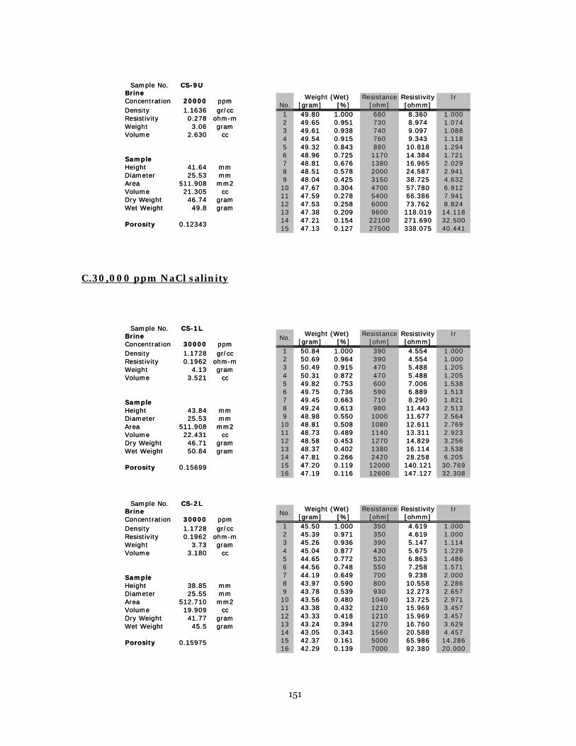
151

C.30,000 ppm NaCl salinity

Sample No. CS-9UBrine Concentration 20000 ppmDensity 1.1636 gr/ccResistivity 0.278 ohm-mWeight 3.06 gramVolume 2.630 cc

SampleHeight 41.64 mmDiameter 25.53 mmArea 511.908 mm2Volume 21.305 ccDry Weight 46.74 gramWet Weight 49.8 gram

Porosity 0.12343

Resistance Resistivity IrNo. [gram] [%] [ohm] [ohmm]1 49.80 1.000 680 8.360 1.0002 49.65 0.951 730 8.974 1.0743 49.61 0.938 740 9.097 1.0884 49.54 0.915 760 9.343 1.1185 49.32 0.843 880 10.818 1.2946 48.96 0.725 1170 14.384 1.7217 48.81 0.676 1380 16.965 2.0298 48.51 0.578 2000 24.587 2.9419 48.04 0.425 3150 38.725 4.63210 47.67 0.304 4700 57.780 6.91211 47.59 0.278 5400 66.386 7.94112 47.53 0.258 6000 73.762 8.82413 47.38 0.209 9600 118.019 14.11814 47.21 0.154 22100 271.690 32.50015 47.13 0.127 27500 338.075 40.441

Weight (Wet)

Sample No. CS-9UBrine Concentration 20000 ppmDensity 1.1636 gr/ccResistivity 0.278 ohm-mWeight 3.06 gramVolume 2.630 cc

SampleHeight 41.64 mmDiameter 25.53 mmArea 511.908 mm2Volume 21.305 ccDry Weight 46.74 gramWet Weight 49.8 gram

Porosity 0.12343

Resistance Resistivity IrNo. [gram] [%] [ohm] [ohmm]1 49.80 1.000 680 8.360 1.0002 49.65 0.951 730 8.974 1.0743 49.61 0.938 740 9.097 1.0884 49.54 0.915 760 9.343 1.1185 49.32 0.843 880 10.818 1.2946 48.96 0.725 1170 14.384 1.7217 48.81 0.676 1380 16.965 2.0298 48.51 0.578 2000 24.587 2.9419 48.04 0.425 3150 38.725 4.63210 47.67 0.304 4700 57.780 6.91211 47.59 0.278 5400 66.386 7.94112 47.53 0.258 6000 73.762 8.82413 47.38 0.209 9600 118.019 14.11814 47.21 0.154 22100 271.690 32.50015 47.13 0.127 27500 338.075 40.441

Weight (Wet)

Sample No. CS-1LBrine Concentration 30000 ppmDensity 1.1728 gr/ccResistivity 0.1962 ohm-mWeight 4.13 gramVolume 3.521 cc

SampleHeight 43.84 mmDiameter 25.53 mmArea 511.908 mm2Volume 22.431 ccDry Weight 46.71 gramWet Weight 50.84 gram

Porosity 0.15699

Resistance Resistivity Ir[gram] [%] [ohm] [ohmm]

1 50.84 1.000 390 4.554 1.0002 50.69 0.964 390 4.554 1.0003 50.49 0.915 470 5.488 1.2054 50.31 0.872 470 5.488 1.2055 49.82 0.753 600 7.006 1.5386 49.75 0.736 590 6.889 1.5137 49.45 0.663 710 8.290 1.8218 49.24 0.613 980 11.443 2.5139 48.98 0.550 1000 11.677 2.56410 48.81 0.508 1080 12.611 2.76911 48.73 0.489 1140 13.311 2.92312 48.58 0.453 1270 14.829 3.25613 48.37 0.402 1380 16.114 3.53814 47.81 0.266 2420 28.258 6.20515 47.20 0.119 12000 140.121 30.76916 47.19 0.116 12600 147.127 32.308

Weight (Wet)No.

Sample No. CS-1LBrine Concentration 30000 ppmDensity 1.1728 gr/ccResistivity 0.1962 ohm-mWeight 4.13 gramVolume 3.521 cc

SampleHeight 43.84 mmDiameter 25.53 mmArea 511.908 mm2Volume 22.431 ccDry Weight 46.71 gramWet Weight 50.84 gram

Porosity 0.15699

Resistance Resistivity Ir[gram] [%] [ohm] [ohmm]

1 50.84 1.000 390 4.554 1.0002 50.69 0.964 390 4.554 1.0003 50.49 0.915 470 5.488 1.2054 50.31 0.872 470 5.488 1.2055 49.82 0.753 600 7.006 1.5386 49.75 0.736 590 6.889 1.5137 49.45 0.663 710 8.290 1.8218 49.24 0.613 980 11.443 2.5139 48.98 0.550 1000 11.677 2.56410 48.81 0.508 1080 12.611 2.76911 48.73 0.489 1140 13.311 2.92312 48.58 0.453 1270 14.829 3.25613 48.37 0.402 1380 16.114 3.53814 47.81 0.266 2420 28.258 6.20515 47.20 0.119 12000 140.121 30.76916 47.19 0.116 12600 147.127 32.308

Weight (Wet)No.

Sample No. CS-2LBrine Concentration 30000 ppmDensity 1.1728 gr/ccResistivity 0.1962 ohm-mWeight 3.73 gramVolume 3.180 cc

SampleHeight 38.85 mmDiameter 25.55 mmArea 512.710 mm2Volume 19.909 ccDry Weight 41.77 gramWet Weight 45.5 gram

Porosity 0.15975

Resistance Resistivity Ir[gram] [%] [ohm] [ohmm]

1 45.50 1.000 350 4.619 1.0002 45.39 0.971 350 4.619 1.0003 45.26 0.936 390 5.147 1.1144 45.04 0.877 430 5.675 1.2295 44.65 0.772 520 6.863 1.4866 44.56 0.748 550 7.258 1.5717 44.19 0.649 700 9.238 2.0008 43.97 0.590 800 10.558 2.2869 43.78 0.539 930 12.273 2.65710 43.56 0.480 1040 13.725 2.97111 43.38 0.432 1210 15.969 3.45712 43.33 0.418 1210 15.969 3.45713 43.24 0.394 1270 16.760 3.62914 43.05 0.343 1560 20.588 4.45715 42.37 0.161 5000 65.986 14.28616 42.29 0.139 7000 92.380 20.000

Weight (Wet)No.

Sample No. CS-2LBrine Concentration 30000 ppmDensity 1.1728 gr/ccResistivity 0.1962 ohm-mWeight 3.73 gramVolume 3.180 cc

SampleHeight 38.85 mmDiameter 25.55 mmArea 512.710 mm2Volume 19.909 ccDry Weight 41.77 gramWet Weight 45.5 gram

Porosity 0.15975

Resistance Resistivity Ir[gram] [%] [ohm] [ohmm]

1 45.50 1.000 350 4.619 1.0002 45.39 0.971 350 4.619 1.0003 45.26 0.936 390 5.147 1.1144 45.04 0.877 430 5.675 1.2295 44.65 0.772 520 6.863 1.4866 44.56 0.748 550 7.258 1.5717 44.19 0.649 700 9.238 2.0008 43.97 0.590 800 10.558 2.2869 43.78 0.539 930 12.273 2.65710 43.56 0.480 1040 13.725 2.97111 43.38 0.432 1210 15.969 3.45712 43.33 0.418 1210 15.969 3.45713 43.24 0.394 1270 16.760 3.62914 43.05 0.343 1560 20.588 4.45715 42.37 0.161 5000 65.986 14.28616 42.29 0.139 7000 92.380 20.000

Weight (Wet)No.

152

Sample No. CS-3LBrine Concentration 30000 ppmDensity 1.1728 gr/ccResistivity 0.1962 ohm-mWeight 4.09 gramVolume 3.487 cc

SampleHeight 43.87 mmDiameter 25.52 mmArea 511.507 mm2Volume 22.428 ccDry Weight 47.2 gramWet Weight 51.29 gram

Porosity 0.15549

Resistance Resistivity Ir[gram] [%] [ohm] [ohmm]

1 51.29 1.000 420 4.897 1.0002 51.09 0.951 440 5.130 1.0483 50.84 0.890 500 5.830 1.1904 50.68 0.851 540 6.296 1.2865 50.39 0.780 640 7.462 1.5246 50.32 0.763 630 7.346 1.5007 50.14 0.719 700 8.162 1.6678 49.93 0.667 780 9.094 1.8579 49.64 0.597 940 10.960 2.23810 49.47 0.555 1030 12.009 2.45211 49.31 0.516 1200 13.992 2.85712 49.12 0.469 1290 15.041 3.07113 48.96 0.430 1460 17.023 3.47614 48.65 0.355 1830 21.337 4.35715 47.81 0.149 7800 90.945 18.57116 47.74 0.132 10100 117.762 24.048

Weight (Wet)No.

Sample No. CS-3LBrine Concentration 30000 ppmDensity 1.1728 gr/ccResistivity 0.1962 ohm-mWeight 4.09 gramVolume 3.487 cc

SampleHeight 43.87 mmDiameter 25.52 mmArea 511.507 mm2Volume 22.428 ccDry Weight 47.2 gramWet Weight 51.29 gram

Porosity 0.15549

Resistance Resistivity Ir[gram] [%] [ohm] [ohmm]

1 51.29 1.000 420 4.897 1.0002 51.09 0.951 440 5.130 1.0483 50.84 0.890 500 5.830 1.1904 50.68 0.851 540 6.296 1.2865 50.39 0.780 640 7.462 1.5246 50.32 0.763 630 7.346 1.5007 50.14 0.719 700 8.162 1.6678 49.93 0.667 780 9.094 1.8579 49.64 0.597 940 10.960 2.23810 49.47 0.555 1030 12.009 2.45211 49.31 0.516 1200 13.992 2.85712 49.12 0.469 1290 15.041 3.07113 48.96 0.430 1460 17.023 3.47614 48.65 0.355 1830 21.337 4.35715 47.81 0.149 7800 90.945 18.57116 47.74 0.132 10100 117.762 24.048

Weight (Wet)No.

Sample No. CS-4LBrine Concentration 30000 ppmDensity 1.1728 gr/ccResistivity 0.1962 ohm-mWeight 4.19 gramVolume 3.573 cc

SampleHeight 44.98 mmDiameter 25.52 mmArea 511.507 mm2Volume 22.996 ccDry Weight 47.97 gramWet Weight 52.16 gram

Porosity 0.15536

Resistance Resistivity Ir[gram] [%] [ohm] [ohmm]

1 52.16 1.000 430 4.890 1.0002 52.06 0.976 430 4.890 1.0003 51.91 0.940 460 5.231 1.0704 51.63 0.874 540 6.141 1.2565 50.91 0.702 750 8.529 1.7446 50.86 0.690 800 9.097 1.8607 50.65 0.640 880 10.007 2.0478 50.49 0.601 970 11.031 2.2569 50.23 0.539 1160 13.191 2.69810 50.05 0.496 1260 14.329 2.93011 49.90 0.461 1420 16.148 3.30212 49.75 0.425 1630 18.536 3.79113 49.53 0.372 1810 20.583 4.20914 49.32 0.322 2080 23.653 4.83715 48.50 0.126 12500 142.148 29.07016 48.49 0.124 12400 141.011 28.837

Weight (Wet)No.

Sample No. CS-4LBrine Concentration 30000 ppmDensity 1.1728 gr/ccResistivity 0.1962 ohm-mWeight 4.19 gramVolume 3.573 cc

SampleHeight 44.98 mmDiameter 25.52 mmArea 511.507 mm2Volume 22.996 ccDry Weight 47.97 gramWet Weight 52.16 gram

Porosity 0.15536

Resistance Resistivity Ir[gram] [%] [ohm] [ohmm]

1 52.16 1.000 430 4.890 1.0002 52.06 0.976 430 4.890 1.0003 51.91 0.940 460 5.231 1.0704 51.63 0.874 540 6.141 1.2565 50.91 0.702 750 8.529 1.7446 50.86 0.690 800 9.097 1.8607 50.65 0.640 880 10.007 2.0478 50.49 0.601 970 11.031 2.2569 50.23 0.539 1160 13.191 2.69810 50.05 0.496 1260 14.329 2.93011 49.90 0.461 1420 16.148 3.30212 49.75 0.425 1630 18.536 3.79113 49.53 0.372 1810 20.583 4.20914 49.32 0.322 2080 23.653 4.83715 48.50 0.126 12500 142.148 29.07016 48.49 0.124 12400 141.011 28.837

Weight (Wet)No.

Sample No. CS-5LBrine Concentration 30000 ppmDensity 1.1728 gr/ccResistivity 0.1962 ohm-mWeight 4.02 gramVolume 3.428 cc

SampleHeight 43.87 mmDiameter 25.54 mmArea 512.309 mm2Volume 22.464 ccDry Weight 47.35 gramWet Weight 51.37 gram

Porosity 0.15259

Resistance Resistivity Ir[gram] [%] [ohm] [ohmm]

1 51.37 1.000 420 4.905 1.0002 50.97 0.900 480 5.605 1.1433 50.73 0.841 530 6.189 1.2624 50.53 0.791 600 7.007 1.4295 50.32 0.739 670 7.824 1.5956 50.24 0.719 730 8.525 1.7387 50.05 0.672 810 9.459 1.9298 49.72 0.590 970 11.328 2.3109 49.36 0.500 1260 14.714 3.00010 49.26 0.475 1290 15.064 3.07111 49.07 0.428 1500 17.517 3.57112 48.97 0.403 1540 17.984 3.66713 48.87 0.378 1700 19.852 4.04814 48.54 0.296 2580 30.129 6.14315 47.95 0.149 8400 98.094 20.00016 47.90 0.137 8800 102.765 20.952

Weight (Wet)No.

Sample No. CS-5LBrine Concentration 30000 ppmDensity 1.1728 gr/ccResistivity 0.1962 ohm-mWeight 4.02 gramVolume 3.428 cc

SampleHeight 43.87 mmDiameter 25.54 mmArea 512.309 mm2Volume 22.464 ccDry Weight 47.35 gramWet Weight 51.37 gram

Porosity 0.15259

Resistance Resistivity Ir[gram] [%] [ohm] [ohmm]

1 51.37 1.000 420 4.905 1.0002 50.97 0.900 480 5.605 1.1433 50.73 0.841 530 6.189 1.2624 50.53 0.791 600 7.007 1.4295 50.32 0.739 670 7.824 1.5956 50.24 0.719 730 8.525 1.7387 50.05 0.672 810 9.459 1.9298 49.72 0.590 970 11.328 2.3109 49.36 0.500 1260 14.714 3.00010 49.26 0.475 1290 15.064 3.07111 49.07 0.428 1500 17.517 3.57112 48.97 0.403 1540 17.984 3.66713 48.87 0.378 1700 19.852 4.04814 48.54 0.296 2580 30.129 6.14315 47.95 0.149 8400 98.094 20.00016 47.90 0.137 8800 102.765 20.952

Weight (Wet)No.

153

Sample No. CS-7LBrine Concentration 30000 ppmDensity 1.1728 gr/ccResistivity 0.1962 ohm-mWeight 3.67 gramVolume 3.129 cc

SampleHeight 38.87 mmDiameter 25.53 mmArea 511.908 mm2Volume 19.888 ccDry Weight 41.89 gramWet Weight 45.56 gram

Porosity 0.15735

Resistance Resistivity Ir[gram] [%] [ohm] [ohmm]

1 45.56 1.000 360 4.741 1.0002 45.46 0.973 370 4.873 1.0283 45.37 0.948 390 5.136 1.0834 45.04 0.858 450 5.926 1.2505 44.67 0.757 540 7.112 1.5006 44.59 0.736 550 7.243 1.5287 44.51 0.714 590 7.770 1.6398 44.37 0.676 660 8.692 1.8339 44.01 0.578 830 10.931 2.30610 43.83 0.529 950 12.511 2.63911 43.60 0.466 1110 14.618 3.08312 43.38 0.406 1250 16.462 3.47213 43.32 0.390 1290 16.989 3.58314 42.76 0.237 2520 33.188 7.00015 42.44 0.150 5400 71.117 15.00016 42.41 0.142 6200 81.652 17.222

Weight (Wet)No.

Sample No. CS-7LBrine Concentration 30000 ppmDensity 1.1728 gr/ccResistivity 0.1962 ohm-mWeight 3.67 gramVolume 3.129 cc

SampleHeight 38.87 mmDiameter 25.53 mmArea 511.908 mm2Volume 19.888 ccDry Weight 41.89 gramWet Weight 45.56 gram

Porosity 0.15735

Resistance Resistivity Ir[gram] [%] [ohm] [ohmm]

1 45.56 1.000 360 4.741 1.0002 45.46 0.973 370 4.873 1.0283 45.37 0.948 390 5.136 1.0834 45.04 0.858 450 5.926 1.2505 44.67 0.757 540 7.112 1.5006 44.59 0.736 550 7.243 1.5287 44.51 0.714 590 7.770 1.6398 44.37 0.676 660 8.692 1.8339 44.01 0.578 830 10.931 2.30610 43.83 0.529 950 12.511 2.63911 43.60 0.466 1110 14.618 3.08312 43.38 0.406 1250 16.462 3.47213 43.32 0.390 1290 16.989 3.58314 42.76 0.237 2520 33.188 7.00015 42.44 0.150 5400 71.117 15.00016 42.41 0.142 6200 81.652 17.222

Weight (Wet)No.

Sample No. CS-8LBrine Concentration 30000 ppmDensity 1.1728 gr/ccResistivity 0.1962 ohm-mWeight 3.55 gramVolume 3.027 cc

SampleHeight 38.29 mmDiameter 25.55 mmArea 512.710 mm2Volume 19.622 ccDry Weight 41.07 gramWet Weight 44.62 gram

Porosity 0.15427

Resistance Resistivity Ir[gram] [%] [ohm] [ohmm]

1 44.62 1.000 350 4.687 1.0002 44.47 0.958 380 5.088 1.0863 44.28 0.904 410 5.490 1.1714 44.15 0.868 480 6.427 1.3715 43.59 0.710 600 8.034 1.7146 43.56 0.701 600 8.034 1.7147 43.42 0.662 670 8.971 1.9148 43.32 0.634 750 10.043 2.1439 43.10 0.572 870 11.649 2.48610 42.92 0.521 950 12.721 2.71411 42.82 0.493 1030 13.792 2.94312 42.72 0.465 1090 14.595 3.11413 42.58 0.425 1220 16.336 3.48614 42.12 0.296 1920 25.709 5.48615 41.59 0.146 6700 89.714 19.14316 41.55 0.135 8000 107.121 22.857

Weight (Wet)No.

Sample No. CS-8LBrine Concentration 30000 ppmDensity 1.1728 gr/ccResistivity 0.1962 ohm-mWeight 3.55 gramVolume 3.027 cc

SampleHeight 38.29 mmDiameter 25.55 mmArea 512.710 mm2Volume 19.622 ccDry Weight 41.07 gramWet Weight 44.62 gram

Porosity 0.15427

Resistance Resistivity Ir[gram] [%] [ohm] [ohmm]

1 44.62 1.000 350 4.687 1.0002 44.47 0.958 380 5.088 1.0863 44.28 0.904 410 5.490 1.1714 44.15 0.868 480 6.427 1.3715 43.59 0.710 600 8.034 1.7146 43.56 0.701 600 8.034 1.7147 43.42 0.662 670 8.971 1.9148 43.32 0.634 750 10.043 2.1439 43.10 0.572 870 11.649 2.48610 42.92 0.521 950 12.721 2.71411 42.82 0.493 1030 13.792 2.94312 42.72 0.465 1090 14.595 3.11413 42.58 0.425 1220 16.336 3.48614 42.12 0.296 1920 25.709 5.48615 41.59 0.146 6700 89.714 19.14316 41.55 0.135 8000 107.121 22.857

Weight (Wet)No.

Sample No. CS-9LBrine Concentration 30000 ppmDensity 1.1728 gr/ccResistivity 0.1962 ohm-mWeight 3.73 gramVolume 3.180 cc

SampleHeight 42.18 mmDiameter 25.55 mmArea 512.710 mm2Volume 21.615 ccDry Weight 44.72 gramWet Weight 48.45 gram

Porosity 0.14714

Resistance Resistivity Ir[gram] [%] [ohm] [ohmm]

1 48.45 1.000 420 5.105 1.0002 48.32 0.965 420 5.105 1.0003 48.22 0.938 450 5.470 1.0714 48.09 0.903 480 5.835 1.1435 47.58 0.767 650 7.901 1.5486 47.48 0.740 640 7.779 1.5247 47.33 0.700 830 10.089 1.9768 47.03 0.619 880 10.697 2.0959 46.57 0.496 1210 14.708 2.88110 46.56 0.493 1170 14.222 2.78611 46.45 0.464 1250 15.194 2.97612 46.28 0.418 1450 17.625 3.45213 46.18 0.391 1520 18.476 3.61914 45.86 0.306 2070 25.161 4.92915 45.25 0.142 8000 97.242 19.04816 45.21 0.131 10000 121.553 23.810

Weight (Wet)No.

Sample No. CS-9LBrine Concentration 30000 ppmDensity 1.1728 gr/ccResistivity 0.1962 ohm-mWeight 3.73 gramVolume 3.180 cc

SampleHeight 42.18 mmDiameter 25.55 mmArea 512.710 mm2Volume 21.615 ccDry Weight 44.72 gramWet Weight 48.45 gram

Porosity 0.14714

Resistance Resistivity Ir[gram] [%] [ohm] [ohmm]

1 48.45 1.000 420 5.105 1.0002 48.32 0.965 420 5.105 1.0003 48.22 0.938 450 5.470 1.0714 48.09 0.903 480 5.835 1.1435 47.58 0.767 650 7.901 1.5486 47.48 0.740 640 7.779 1.5247 47.33 0.700 830 10.089 1.9768 47.03 0.619 880 10.697 2.0959 46.57 0.496 1210 14.708 2.88110 46.56 0.493 1170 14.222 2.78611 46.45 0.464 1250 15.194 2.97612 46.28 0.418 1450 17.625 3.45213 46.18 0.391 1520 18.476 3.61914 45.86 0.306 2070 25.161 4.92915 45.25 0.142 8000 97.242 19.04816 45.21 0.131 10000 121.553 23.810

Weight (Wet)No.

154

Sample No. CS-1UBrine Concentration 30000 ppmDensity 1.1728 gr/ccResistivity 0.1962 ohm-mWeight 3.16 gramVolume 2.694 cc

SampleHeight 42.75 mmDiameter 25.51 mmArea 511.106 mm2Volume 21.839 ccDry Weight 46.56 gramWet Weight 49.72 gram

Porosity 0.12338

Resistance Resistivity IrNo. [gram] [%] [ohm] [ohmm]1 49.72 1.000 620 7.413 1.0002 49.27 0.858 840 10.043 1.3553 49.11 0.807 1000 11.956 1.6134 48.75 0.693 1310 15.662 2.1135 48.71 0.680 1380 16.499 2.2266 48.22 0.525 2600 31.085 4.1947 47.16 0.190 14700 175.749 23.7108 46.83 0.085 60000 717.341 96.7749 46.77 0.066 96000 1147.746 154.839

Weight (Wet)

Sample No. CS-1UBrine Concentration 30000 ppmDensity 1.1728 gr/ccResistivity 0.1962 ohm-mWeight 3.16 gramVolume 2.694 cc

SampleHeight 42.75 mmDiameter 25.51 mmArea 511.106 mm2Volume 21.839 ccDry Weight 46.56 gramWet Weight 49.72 gram

Porosity 0.12338

Resistance Resistivity IrNo. [gram] [%] [ohm] [ohmm]1 49.72 1.000 620 7.413 1.0002 49.27 0.858 840 10.043 1.3553 49.11 0.807 1000 11.956 1.6134 48.75 0.693 1310 15.662 2.1135 48.71 0.680 1380 16.499 2.2266 48.22 0.525 2600 31.085 4.1947 47.16 0.190 14700 175.749 23.7108 46.83 0.085 60000 717.341 96.7749 46.77 0.066 96000 1147.746 154.839

Weight (Wet)

Sample No. CS-2UBrine Concentration 30000 ppmDensity 1.1728 gr/ccResistivity 0.1962 ohm-mWeight 3.38 gramVolume 2.882 cc

SampleHeight 44.98 mmDiameter 25.51 mmArea 511.106 mm2Volume 22.978 ccDry Weight 49.55 gramWet Weight 52.93 gram

Porosity 0.12542

Resistance Resistivity IrNo. [gram] [%] [ohm] [ohmm]1 52.93 1.000 660 7.500 1.0002 52.22 0.790 990 11.249 1.5003 52.13 0.763 1260 14.317 1.9094 51.91 0.698 1320 14.999 2.0005 51.80 0.666 1480 16.817 2.2426 50.58 0.305 6300 71.587 9.5457 50.08 0.157 15600 177.262 23.6368 49.78 0.068 68000 772.681 103.0309 49.74 0.056 98000 1113.570 148.485

Weight (Wet)

Sample No. CS-2UBrine Concentration 30000 ppmDensity 1.1728 gr/ccResistivity 0.1962 ohm-mWeight 3.38 gramVolume 2.882 cc

SampleHeight 44.98 mmDiameter 25.51 mmArea 511.106 mm2Volume 22.978 ccDry Weight 49.55 gramWet Weight 52.93 gram

Porosity 0.12542

Resistance Resistivity IrNo. [gram] [%] [ohm] [ohmm]1 52.93 1.000 660 7.500 1.0002 52.22 0.790 990 11.249 1.5003 52.13 0.763 1260 14.317 1.9094 51.91 0.698 1320 14.999 2.0005 51.80 0.666 1480 16.817 2.2426 50.58 0.305 6300 71.587 9.5457 50.08 0.157 15600 177.262 23.6368 49.78 0.068 68000 772.681 103.0309 49.74 0.056 98000 1113.570 148.485

Weight (Wet)

Sample No. CS-3UBrine Concentration 30000 ppmDensity 1.1728 gr/ccResistivity 0.1962 ohm-mWeight 3.37 gramVolume 2.873 cc

SampleHeight 45.56 mmDiameter 25.52 mmArea 511.507 mm2Volume 23.292 ccDry Weight 50.48 gramWet Weight 53.85 gram

Porosity 0.12336

Resistance Resistivity IrNo. [gram] [%] [ohm] [ohmm]1 53.85 1.000 700 7.859 1.0002 53.73 0.964 730 8.196 1.0433 53.49 0.893 840 9.431 1.2004 53.14 0.789 1060 11.901 1.5145 53.05 0.763 1120 12.574 1.6006 52.32 0.546 2380 26.720 3.4007 51.60 0.332 4200 47.154 6.0008 50.75 0.080 44000 493.992 62.8579 50.68 0.059 75000 842.032 107.143

Weight (Wet)

Sample No. CS-3UBrine Concentration 30000 ppmDensity 1.1728 gr/ccResistivity 0.1962 ohm-mWeight 3.37 gramVolume 2.873 cc

SampleHeight 45.56 mmDiameter 25.52 mmArea 511.507 mm2Volume 23.292 ccDry Weight 50.48 gramWet Weight 53.85 gram

Porosity 0.12336

Resistance Resistivity IrNo. [gram] [%] [ohm] [ohmm]1 53.85 1.000 700 7.859 1.0002 53.73 0.964 730 8.196 1.0433 53.49 0.893 840 9.431 1.2004 53.14 0.789 1060 11.901 1.5145 53.05 0.763 1120 12.574 1.6006 52.32 0.546 2380 26.720 3.4007 51.60 0.332 4200 47.154 6.0008 50.75 0.080 44000 493.992 62.8579 50.68 0.059 75000 842.032 107.143

Weight (Wet)

155

Sample No. CS-5UBrine Concentration 30000 ppmDensity 1.1728 gr/ccResistivity 0.1962 ohm-mWeight 3.35 gramVolume 2.856 cc

SampleHeight 45.55 mmDiameter 25.52 mmArea 511.507 mm2Volume 23.287 ccDry Weight 50.62 gramWet Weight 53.97 gram

Porosity 0.12266

Resistance Resistivity IrNo. [gram] [%] [ohm] [ohmm]1 53.97 1.000 710 7.973 1.0002 53.73 0.928 780 8.759 1.0993 53.69 0.916 820 9.208 1.1554 53.38 0.824 1010 11.342 1.4235 53.17 0.761 1170 13.139 1.6486 52.70 0.621 1920 21.561 2.7047 51.42 0.239 10200 114.542 14.3668 50.92 0.090 42000 471.642 59.1559 50.87 0.075 64000 718.692 90.141

Weight (Wet)

Sample No. CS-5UBrine Concentration 30000 ppmDensity 1.1728 gr/ccResistivity 0.1962 ohm-mWeight 3.35 gramVolume 2.856 cc

SampleHeight 45.55 mmDiameter 25.52 mmArea 511.507 mm2Volume 23.287 ccDry Weight 50.62 gramWet Weight 53.97 gram

Porosity 0.12266

Resistance Resistivity IrNo. [gram] [%] [ohm] [ohmm]1 53.97 1.000 710 7.973 1.0002 53.73 0.928 780 8.759 1.0993 53.69 0.916 820 9.208 1.1554 53.38 0.824 1010 11.342 1.4235 53.17 0.761 1170 13.139 1.6486 52.70 0.621 1920 21.561 2.7047 51.42 0.239 10200 114.542 14.3668 50.92 0.090 42000 471.642 59.1559 50.87 0.075 64000 718.692 90.141

Weight (Wet)

Sample No. CS-7UBrine Concentration 30000 ppmDensity 1.1728 gr/ccResistivity 0.1962 ohm-mWeight 3.14 gramVolume 2.677 cc

SampleHeight 43.86 mmDiameter 25.51 mmArea 511.106 mm2Volume 22.406 ccDry Weight 48.48 gramWet Weight 51.62 gram

Porosity 0.11949

Resistance Resistivity IrNo. [gram] [%] [ohm] [ohmm]1 51.62 1.000 690 8.041 1.0002 51.44 0.943 750 8.740 1.0873 51.33 0.908 790 9.206 1.1454 50.91 0.774 1120 13.051 1.6235 50.72 0.713 1300 15.149 1.8846 49.71 0.392 4300 50.108 6.2327 49.15 0.213 10600 123.523 15.3628 48.70 0.070 62000 722.493 89.8559 48.66 0.057 92000 1072.087 133.333

Weigh (Wet)

Sample No. CS-7UBrine Concentration 30000 ppmDensity 1.1728 gr/ccResistivity 0.1962 ohm-mWeight 3.14 gramVolume 2.677 cc

SampleHeight 43.86 mmDiameter 25.51 mmArea 511.106 mm2Volume 22.406 ccDry Weight 48.48 gramWet Weight 51.62 gram

Porosity 0.11949

Resistance Resistivity IrNo. [gram] [%] [ohm] [ohmm]1 51.62 1.000 690 8.041 1.0002 51.44 0.943 750 8.740 1.0873 51.33 0.908 790 9.206 1.1454 50.91 0.774 1120 13.051 1.6235 50.72 0.713 1300 15.149 1.8846 49.71 0.392 4300 50.108 6.2327 49.15 0.213 10600 123.523 15.3628 48.70 0.070 62000 722.493 89.8559 48.66 0.057 92000 1072.087 133.333

Weigh (Wet)

Sample No. CS-8UBrine Concentration 30000 ppmDensity 1.1728 gr/ccResistivity 0.1962 ohm-mWeight 2.36 gramVolume 2.012 cc

SampleHeight 37.77 mmDiameter 25.51 mmArea 511.106 mm2Volume 19.295 ccDry Weight 43.67 gramWet Weight 46.03 gram

Porosity 0.10429

Resistance Resistivity IrNo. [gram] [%] [ohm] [ohmm]1 46.03 1.000 780 10.555 1.0002 45.96 0.970 810 10.961 1.0383 45.80 0.903 950 12.855 1.2184 45.54 0.792 1170 15.833 1.5005 45.48 0.767 1230 16.644 1.5776 45.05 0.585 2340 31.665 3.0007 44.51 0.356 4400 59.541 5.6418 43.87 0.085 41000 554.814 52.5649 43.83 0.068 61000 825.455 78.205

Weght (Wet)

Sample No. CS-8UBrine Concentration 30000 ppmDensity 1.1728 gr/ccResistivity 0.1962 ohm-mWeight 2.36 gramVolume 2.012 cc

SampleHeight 37.77 mmDiameter 25.51 mmArea 511.106 mm2Volume 19.295 ccDry Weight 43.67 gramWet Weight 46.03 gram

Porosity 0.10429

Resistance Resistivity IrNo. [gram] [%] [ohm] [ohmm]1 46.03 1.000 780 10.555 1.0002 45.96 0.970 810 10.961 1.0383 45.80 0.903 950 12.855 1.2184 45.54 0.792 1170 15.833 1.5005 45.48 0.767 1230 16.644 1.5776 45.05 0.585 2340 31.665 3.0007 44.51 0.356 4400 59.541 5.6418 43.87 0.085 41000 554.814 52.5649 43.83 0.068 61000 825.455 78.205

Weght (Wet)

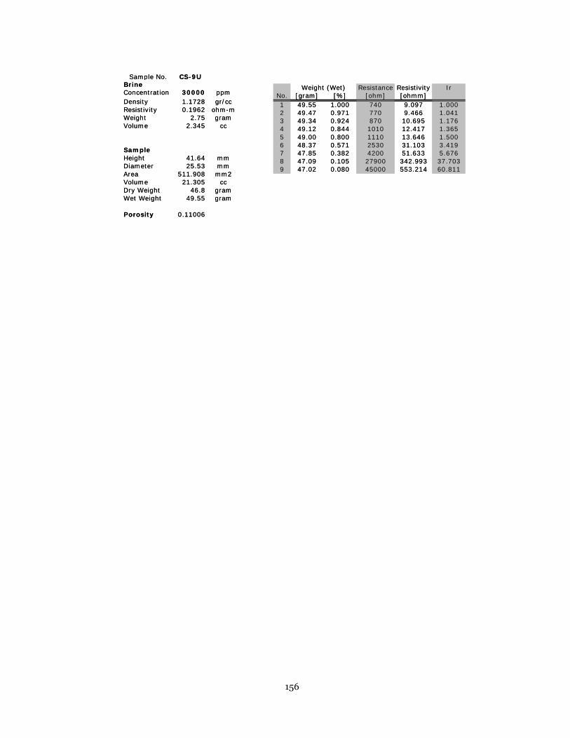
156

Sample No. CS-9UBrine Concentration 30000 ppmDensity 1.1728 gr/ccResistivity 0.1962 ohm-mWeight 2.75 gramVolume 2.345 cc

SampleHeight 41.64 mmDiameter 25.53 mmArea 511.908 mm2Volume 21.305 ccDry Weight 46.8 gramWet Weight 49.55 gram

Porosity 0.11006

Resistance Resistivity IrNo. [gram] [%] [ohm] [ohmm]1 49.55 1.000 740 9.097 1.0002 49.47 0.971 770 9.466 1.0413 49.34 0.924 870 10.695 1.1764 49.12 0.844 1010 12.417 1.3655 49.00 0.800 1110 13.646 1.5006 48.37 0.571 2530 31.103 3.4197 47.85 0.382 4200 51.633 5.6768 47.09 0.105 27900 342.993 37.7039 47.02 0.080 45000 553.214 60.811

Weight (Wet)

Sample No. CS-9UBrine Concentration 30000 ppmDensity 1.1728 gr/ccResistivity 0.1962 ohm-mWeight 2.75 gramVolume 2.345 cc

SampleHeight 41.64 mmDiameter 25.53 mmArea 511.908 mm2Volume 21.305 ccDry Weight 46.8 gramWet Weight 49.55 gram

Porosity 0.11006

Resistance Resistivity IrNo. [gram] [%] [ohm] [ohmm]1 49.55 1.000 740 9.097 1.0002 49.47 0.971 770 9.466 1.0413 49.34 0.924 870 10.695 1.1764 49.12 0.844 1010 12.417 1.3655 49.00 0.800 1110 13.646 1.5006 48.37 0.571 2530 31.103 3.4197 47.85 0.382 4200 51.633 5.6768 47.09 0.105 27900 342.993 37.7039 47.02 0.080 45000 553.214 60.811

Weight (Wet)

157

APPENDIX C DATA OF SHALE ELECTRICAL MEASUREMENT

158

A. 3,000 ppm NaCl Salinity

Sample No. SH-1Brine Concentration 3000 ppmDensity 1.1504 gr/ccResistivity 1.342 ohm-mWeight 0.96 gramVolume 0.834 cc

SampleHeight 18.87 mmDiameter 25.54 mmArea 512.309 mm2Volume 9.662 ccDry Weight 22.26 gramWet Weight 23.22 gram

Porosity 0.08637

Resistance Resistivity IrNo. [gram] [%] [ohm] [ohmm]1 23.22 1.000 1090 29.593 1.0002 23.09 0.865 1140 30.950 1.0463 22.99 0.760 1450 39.367 1.3304 22.77 0.531 1940 52.670 1.7805 22.64 0.396 2480 67.330 2.2756 22.57 0.323 3030 82.263 2.7807 22.46 0.208 6100 165.611 5.5968 22.43 0.177 7800 211.765 7.1569 22.42 0.167 8100 219.910 7.43110 22.40 0.146 10600 287.783 9.72511 22.40 0.146 10800 293.213 9.908

Weight (Wet)Sample No. SH-1

Brine Concentration 3000 ppmDensity 1.1504 gr/ccResistivity 1.342 ohm-mWeight 0.96 gramVolume 0.834 cc

SampleHeight 18.87 mmDiameter 25.54 mmArea 512.309 mm2Volume 9.662 ccDry Weight 22.26 gramWet Weight 23.22 gram

Porosity 0.08637

Resistance Resistivity IrNo. [gram] [%] [ohm] [ohmm]1 23.22 1.000 1090 29.593 1.0002 23.09 0.865 1140 30.950 1.0463 22.99 0.760 1450 39.367 1.3304 22.77 0.531 1940 52.670 1.7805 22.64 0.396 2480 67.330 2.2756 22.57 0.323 3030 82.263 2.7807 22.46 0.208 6100 165.611 5.5968 22.43 0.177 7800 211.765 7.1569 22.42 0.167 8100 219.910 7.43110 22.40 0.146 10600 287.783 9.72511 22.40 0.146 10800 293.213 9.908

Weight (Wet)

Sample No. SH-2Brine Concentration 3000 ppmDensity 1.1504 gr/ccResistivity 1.342 ohm-mWeight 1 gramVolume 0.869 cc

SampleHeight 19.95 mmDiameter 25.53 mmArea 511.908 mm2Volume 10.207 ccDry Weight 23.35 gramWet Weight 24.35 gram

Porosity 0.08516

Resistance Resistivity IrNo. [gram] [%] [ohm] [ohmm]1 24.35 1.000 1160 29.765 1.0002 24.17 0.820 1380 35.410 1.1903 24.09 0.740 1650 42.338 1.4224 23.83 0.480 2320 59.530 2.0005 23.72 0.370 2910 74.669 2.5096 23.68 0.330 3400 87.242 2.9317 23.55 0.200 7600 195.012 6.5528 23.53 0.180 9800 251.463 8.4489 23.52 0.170 10000 256.595 8.62110 23.49 0.140 14800 379.761 12.75911 23.49 0.140 14900 382.327 12.845

Weight (Wet)Sample No. SH-2

Brine Concentration 3000 ppmDensity 1.1504 gr/ccResistivity 1.342 ohm-mWeight 1 gramVolume 0.869 cc

SampleHeight 19.95 mmDiameter 25.53 mmArea 511.908 mm2Volume 10.207 ccDry Weight 23.35 gramWet Weight 24.35 gram

Porosity 0.08516

Resistance Resistivity IrNo. [gram] [%] [ohm] [ohmm]1 24.35 1.000 1160 29.765 1.0002 24.17 0.820 1380 35.410 1.1903 24.09 0.740 1650 42.338 1.4224 23.83 0.480 2320 59.530 2.0005 23.72 0.370 2910 74.669 2.5096 23.68 0.330 3400 87.242 2.9317 23.55 0.200 7600 195.012 6.5528 23.53 0.180 9800 251.463 8.4489 23.52 0.170 10000 256.595 8.62110 23.49 0.140 14800 379.761 12.75911 23.49 0.140 14900 382.327 12.845

Weight (Wet)

Sample No. SH-3Brine Concentration 3000 ppmDensity 1.1504 gr/ccResistivity 1.342 ohm-mWeight 0.97 gramVolume 0.843 cc

SampleHeight 18.87 mmDiameter 25.55 mmArea 512.710 mm2Volume 9.670 ccDry Weight 22.58 gramWet Weight 23.55 gram

Porosity 0.0872

Resistance Resistivity IrNo. [gram] [%] [ohm] [ohmm]1 23.55 1.000 1110 30.159 1.0002 23.43 0.876 1210 32.876 1.0903 23.34 0.784 1390 37.767 1.2524 23.01 0.443 2270 61.677 2.0455 22.92 0.351 2870 77.980 2.5866 22.88 0.309 3400 92.380 3.0637 22.79 0.216 5700 154.873 5.1358 22.75 0.175 8800 239.102 7.9289 22.74 0.165 9100 247.253 8.19810 22.71 0.134 14800 402.125 13.33311 22.71 0.134 14300 388.540 12.883

Weight (Wet)Sample No. SH-3

Brine Concentration 3000 ppmDensity 1.1504 gr/ccResistivity 1.342 ohm-mWeight 0.97 gramVolume 0.843 cc

SampleHeight 18.87 mmDiameter 25.55 mmArea 512.710 mm2Volume 9.670 ccDry Weight 22.58 gramWet Weight 23.55 gram

Porosity 0.0872

Resistance Resistivity IrNo. [gram] [%] [ohm] [ohmm]1 23.55 1.000 1110 30.159 1.0002 23.43 0.876 1210 32.876 1.0903 23.34 0.784 1390 37.767 1.2524 23.01 0.443 2270 61.677 2.0455 22.92 0.351 2870 77.980 2.5866 22.88 0.309 3400 92.380 3.0637 22.79 0.216 5700 154.873 5.1358 22.75 0.175 8800 239.102 7.9289 22.74 0.165 9100 247.253 8.19810 22.71 0.134 14800 402.125 13.33311 22.71 0.134 14300 388.540 12.883

Weight (Wet)

159

Sample No. SH-4Brine Concentration 3000 ppmDensity 1.1504 gr/ccResistivity 1.342 ohm-mWeight 0.85 gramVolume 0.739 cc

SampleHeight 17.75 mmDiameter 25.54 mmArea 512.309 mm2Volume 9.089 ccDry Weight 21.28 gramWet Weight 22.13 gram

Porosity 0.08129

Resistance Resistivity IrNo. [gram] [%] [ohm] [ohmm]1 22.13 1.000 780 22.513 1.0002 21.99 0.835 950 27.419 1.2183 21.87 0.694 1050 30.306 1.3464 21.48 0.235 3030 87.453 3.8855 21.45 0.200 3800 109.677 4.8726 21.44 0.188 4100 118.336 5.2567 21.43 0.176 4700 135.654 6.0268 21.42 0.165 5300 152.971 6.7959 21.41 0.153 5500 158.744 7.05110 21.39 0.129 7500 216.468 9.61511 21.39 0.129 7400 213.582 9.487

Weight (Wet)Sample No. SH-4

Brine Concentration 3000 ppmDensity 1.1504 gr/ccResistivity 1.342 ohm-mWeight 0.85 gramVolume 0.739 cc

SampleHeight 17.75 mmDiameter 25.54 mmArea 512.309 mm2Volume 9.089 ccDry Weight 21.28 gramWet Weight 22.13 gram

Porosity 0.08129

Resistance Resistivity IrNo. [gram] [%] [ohm] [ohmm]1 22.13 1.000 780 22.513 1.0002 21.99 0.835 950 27.419 1.2183 21.87 0.694 1050 30.306 1.3464 21.48 0.235 3030 87.453 3.8855 21.45 0.200 3800 109.677 4.8726 21.44 0.188 4100 118.336 5.2567 21.43 0.176 4700 135.654 6.0268 21.42 0.165 5300 152.971 6.7959 21.41 0.153 5500 158.744 7.05110 21.39 0.129 7500 216.468 9.61511 21.39 0.129 7400 213.582 9.487

Weight (Wet)

Sample No. SH-5Brine Concentration 3000 ppmDensity 1.1504 gr/ccResistivity 1.342 ohm-mWeight 0.83 gramVolume 0.721 cc

SampleHeight 18.85 mmDiameter 25.54 mmArea 512.309 mm2Volume 9.652 ccDry Weight 22.45 gramWet Weight 23.28 gram

Porosity 0.07475

Resistance Resistivity IrNo. [gram] [%] [ohm] [ohmm]1 23.28 1.000 1190 32.342 1.0002 23.20 0.904 1300 35.332 1.0923 23.09 0.771 1510 41.039 1.2694 22.75 0.361 2370 64.412 1.9925 22.68 0.277 3040 82.622 2.5556 22.64 0.229 3900 105.995 3.2777 22.58 0.157 5900 160.351 4.9588 22.56 0.133 7800 211.990 6.5559 22.55 0.120 7900 214.708 6.63910 22.53 0.096 11600 315.267 9.74811 22.53 0.096 10700 290.806 8.992

Weight (Wet)Sample No. SH-5

Brine Concentration 3000 ppmDensity 1.1504 gr/ccResistivity 1.342 ohm-mWeight 0.83 gramVolume 0.721 cc

SampleHeight 18.85 mmDiameter 25.54 mmArea 512.309 mm2Volume 9.652 ccDry Weight 22.45 gramWet Weight 23.28 gram

Porosity 0.07475

Resistance Resistivity IrNo. [gram] [%] [ohm] [ohmm]1 23.28 1.000 1190 32.342 1.0002 23.20 0.904 1300 35.332 1.0923 23.09 0.771 1510 41.039 1.2694 22.75 0.361 2370 64.412 1.9925 22.68 0.277 3040 82.622 2.5556 22.64 0.229 3900 105.995 3.2777 22.58 0.157 5900 160.351 4.9588 22.56 0.133 7800 211.990 6.5559 22.55 0.120 7900 214.708 6.63910 22.53 0.096 11600 315.267 9.74811 22.53 0.096 10700 290.806 8.992

Weight (Wet)

Sample No. SH-6Brine Concentration 3000 ppmDensity 1.1504 gr/ccResistivity 1.342 ohm-mWeight 0.74 gramVolume 0.643 cc

SampleHeight 16.65 mmDiameter 25.53 mmArea 511.908 mm2Volume 8.519 ccDry Weight 19.71 gramWet Weight 20.45 gram

Porosity 0.07551

Resistance Resistivity IrNo. [gram] [%] [ohm] [ohmm]1 20.45 1.000 1040 31.975 1.0002 20.34 0.851 1190 36.587 1.1443 20.20 0.662 1510 46.425 1.4524 19.93 0.297 2460 75.633 2.3655 19.91 0.270 2650 81.475 2.5486 19.90 0.257 2960 91.006 2.8467 19.82 0.149 5400 166.024 5.1928 19.80 0.122 7000 215.216 6.7319 19.80 0.122 7100 218.291 6.82710 19.78 0.095 10300 316.676 9.90411 19.78 0.095 10200 313.601 9.808

Weight (Wet)

Sample No. SH-6Brine Concentration 3000 ppmDensity 1.1504 gr/ccResistivity 1.342 ohm-mWeight 0.74 gramVolume 0.643 cc

SampleHeight 16.65 mmDiameter 25.53 mmArea 511.908 mm2Volume 8.519 ccDry Weight 19.71 gramWet Weight 20.45 gram

Porosity 0.07551

Resistance Resistivity IrNo. [gram] [%] [ohm] [ohmm]1 20.45 1.000 1040 31.975 1.0002 20.34 0.851 1190 36.587 1.1443 20.20 0.662 1510 46.425 1.4524 19.93 0.297 2460 75.633 2.3655 19.91 0.270 2650 81.475 2.5486 19.90 0.257 2960 91.006 2.8467 19.82 0.149 5400 166.024 5.1928 19.80 0.122 7000 215.216 6.7319 19.80 0.122 7100 218.291 6.82710 19.78 0.095 10300 316.676 9.90411 19.78 0.095 10200 313.601 9.808

Weight (Wet)

160

Sample No. SH-7Brine Concentration 3000 ppmDensity 1.1504 gr/ccResistivity 1.342 ohm-mWeight 0.78 gramVolume 0.678 cc

SampleHeight 17.77 mmDiameter 25.54 mmArea 512.309 mm2Volume 9.099 ccDry Weight 21.85 gramWet Weight 22.63 gram

Porosity 0.07452

Resistance Resistivity IrNo. [gram] [%] [ohm] [ohmm]1 22.63 1.000 670 19.316 1.0002 22.54 0.885 710 20.469 1.0603 22.41 0.718 960 27.677 1.4334 22.29 0.564 1480 42.668 2.2095 22.19 0.436 1970 56.795 2.9406 22.18 0.423 2110 60.831 3.1497 22.07 0.282 3600 103.788 5.3738 22.04 0.244 4500 129.735 6.7169 22.03 0.231 4600 132.618 6.86610 22.01 0.205 6100 175.863 9.10411 22.01 0.205 6100 175.863 9.104

Weight (Wet)Sample No. SH-7

Brine Concentration 3000 ppmDensity 1.1504 gr/ccResistivity 1.342 ohm-mWeight 0.78 gramVolume 0.678 cc

SampleHeight 17.77 mmDiameter 25.54 mmArea 512.309 mm2Volume 9.099 ccDry Weight 21.85 gramWet Weight 22.63 gram

Porosity 0.07452

Resistance Resistivity IrNo. [gram] [%] [ohm] [ohmm]1 22.63 1.000 670 19.316 1.0002 22.54 0.885 710 20.469 1.0603 22.41 0.718 960 27.677 1.4334 22.29 0.564 1480 42.668 2.2095 22.19 0.436 1970 56.795 2.9406 22.18 0.423 2110 60.831 3.1497 22.07 0.282 3600 103.788 5.3738 22.04 0.244 4500 129.735 6.7169 22.03 0.231 4600 132.618 6.86610 22.01 0.205 6100 175.863 9.10411 22.01 0.205 6100 175.863 9.104

Weight (Wet)

Sample No. SH-8Brine Concentration 3000 ppmDensity 1.1504 gr/ccResistivity 1.342 ohm-mWeight 0.78 gramVolume 0.678 cc

SampleHeight 18.32 mmDiameter 25.52 mmArea 511.507 mm2Volume 9.366 ccDry Weight 22.66 gramWet Weight 23.44 gram

Porosity 0.07239

Resistance Resistivity IrNo. [gram] [%] [ohm] [ohmm]1 23.44 1.000 740 20.661 1.0002 23.34 0.872 790 22.057 1.0683 23.25 0.756 980 27.362 1.3244 22.96 0.385 2160 60.309 2.9195 22.91 0.321 2680 74.827 3.6226 22.88 0.282 3020 84.320 4.0817 22.85 0.244 3900 108.891 5.2708 22.83 0.218 4600 128.435 6.2169 22.83 0.218 4600 128.435 6.21610 22.80 0.179 6100 170.316 8.24311 22.80 0.179 6200 173.108 8.378

Weight (Wet)

Sample No. SH-8Brine Concentration 3000 ppmDensity 1.1504 gr/ccResistivity 1.342 ohm-mWeight 0.78 gramVolume 0.678 cc

SampleHeight 18.32 mmDiameter 25.52 mmArea 511.507 mm2Volume 9.366 ccDry Weight 22.66 gramWet Weight 23.44 gram

Porosity 0.07239

Resistance Resistivity IrNo. [gram] [%] [ohm] [ohmm]1 23.44 1.000 740 20.661 1.0002 23.34 0.872 790 22.057 1.0683 23.25 0.756 980 27.362 1.3244 22.96 0.385 2160 60.309 2.9195 22.91 0.321 2680 74.827 3.6226 22.88 0.282 3020 84.320 4.0817 22.85 0.244 3900 108.891 5.2708 22.83 0.218 4600 128.435 6.2169 22.83 0.218 4600 128.435 6.21610 22.80 0.179 6100 170.316 8.24311 22.80 0.179 6200 173.108 8.378

Weight (Wet)

Sample No. SH-9Brine Concentration 3000 ppmDensity 1.1504 gr/ccResistivity 1.342 ohm-mWeight 0.88 gramVolume 0.765 cc

SampleHeight 17.76 mmDiameter 25.53 mmArea 511.908 mm2Volume 9.087 ccDry Weight 21.68 gramWet Weight 22.56 gram

Porosity 0.08418

Resistance Resistivity IrNo. [gram] [%] [ohm] [ohmm]1 22.56 1.000 560 16.141 1.0002 22.46 0.886 600 17.294 1.0713 22.32 0.727 890 25.653 1.5894 22.12 0.500 1800 51.883 3.2145 22.10 0.477 1880 54.188 3.3576 22.06 0.432 2110 60.818 3.7687 21.99 0.352 2910 83.877 5.1968 21.95 0.307 3800 109.530 6.7869 21.93 0.284 3900 112.412 6.96410 21.89 0.239 5500 158.530 9.82111 21.89 0.239 5500 158.530 9.821

Weight (Wet)Sample No. SH-9

Brine Concentration 3000 ppmDensity 1.1504 gr/ccResistivity 1.342 ohm-mWeight 0.88 gramVolume 0.765 cc

SampleHeight 17.76 mmDiameter 25.53 mmArea 511.908 mm2Volume 9.087 ccDry Weight 21.68 gramWet Weight 22.56 gram

Porosity 0.08418

Resistance Resistivity IrNo. [gram] [%] [ohm] [ohmm]1 22.56 1.000 560 16.141 1.0002 22.46 0.886 600 17.294 1.0713 22.32 0.727 890 25.653 1.5894 22.12 0.500 1800 51.883 3.2145 22.10 0.477 1880 54.188 3.3576 22.06 0.432 2110 60.818 3.7687 21.99 0.352 2910 83.877 5.1968 21.95 0.307 3800 109.530 6.7869 21.93 0.284 3900 112.412 6.96410 21.89 0.239 5500 158.530 9.82111 21.89 0.239 5500 158.530 9.821

Weight (Wet)

161

Sample No. SH-10Brine Concentration 3000 ppmDensity 1.1504 gr/ccResistivity 1.342 ohm-mWeight 0.79 gramVolume 0.687 cc

SampleHeight 18.28 mmDiameter 25.53 mmArea 511.908 mm2Volume 9.353 ccDry Weight 21.92 gramWet Weight 22.71 gram

Porosity 0.07342

Resistance Resistivity IrNo. [gram] [%] [ohm] [ohmm]1 22.71 1.000 570 15.962 1.0002 22.60 0.861 620 17.362 1.0883 22.46 0.684 1000 28.004 1.7544 22.23 0.392 1920 53.767 3.3685 22.26 0.430 1730 48.446 3.0356 22.25 0.418 1850 51.807 3.2467 22.17 0.316 2690 75.330 4.7198 22.14 0.278 3400 95.213 5.9659 22.13 0.266 3300 92.412 5.78910 22.10 0.228 4400 123.216 7.71911 22.11 0.241 4300 120.416 7.544

Weight (Wet)

Sample No. SH-10Brine Concentration 3000 ppmDensity 1.1504 gr/ccResistivity 1.342 ohm-mWeight 0.79 gramVolume 0.687 cc

SampleHeight 18.28 mmDiameter 25.53 mmArea 511.908 mm2Volume 9.353 ccDry Weight 21.92 gramWet Weight 22.71 gram

Porosity 0.07342

Resistance Resistivity IrNo. [gram] [%] [ohm] [ohmm]1 22.71 1.000 570 15.962 1.0002 22.60 0.861 620 17.362 1.0883 22.46 0.684 1000 28.004 1.7544 22.23 0.392 1920 53.767 3.3685 22.26 0.430 1730 48.446 3.0356 22.25 0.418 1850 51.807 3.2467 22.17 0.316 2690 75.330 4.7198 22.14 0.278 3400 95.213 5.9659 22.13 0.266 3300 92.412 5.78910 22.10 0.228 4400 123.216 7.71911 22.11 0.241 4300 120.416 7.544

Weight (Wet)

Sample No. SH-11Brine Concentration 3000 ppmDensity 1.1504 gr/ccResistivity 1.342 ohm-mWeight 0.77 gramVolume 0.669 cc

SampleHeight 18.29 mmDiameter 25.53 mmArea 511.908 mm2Volume 9.358 ccDry Weight 22.29 gramWet Weight 23.06 gram

Porosity 0.07152

Resistance Resistivity IrNo. [gram] [%] [ohm] [ohmm]1 23.06 1.000 740 20.711 1.0002 22.93 0.831 810 22.671 1.0953 22.85 0.727 1040 29.108 1.4054 22.59 0.390 2040 57.096 2.7575 22.52 0.299 2610 73.050 3.5276 22.53 0.312 2970 83.125 4.0147 22.46 0.221 4200 117.551 5.6768 22.45 0.208 4600 128.747 6.2169 22.44 0.195 4500 125.948 6.08110 22.42 0.169 6400 179.126 8.64911 22.43 0.182 6100 170.729 8.243

Weight (Wet)

Sample No. SH-11Brine Concentration 3000 ppmDensity 1.1504 gr/ccResistivity 1.342 ohm-mWeight 0.77 gramVolume 0.669 cc

SampleHeight 18.29 mmDiameter 25.53 mmArea 511.908 mm2Volume 9.358 ccDry Weight 22.29 gramWet Weight 23.06 gram

Porosity 0.07152

Resistance Resistivity IrNo. [gram] [%] [ohm] [ohmm]1 23.06 1.000 740 20.711 1.0002 22.93 0.831 810 22.671 1.0953 22.85 0.727 1040 29.108 1.4054 22.59 0.390 2040 57.096 2.7575 22.52 0.299 2610 73.050 3.5276 22.53 0.312 2970 83.125 4.0147 22.46 0.221 4200 117.551 5.6768 22.45 0.208 4600 128.747 6.2169 22.44 0.195 4500 125.948 6.08110 22.42 0.169 6400 179.126 8.64911 22.43 0.182 6100 170.729 8.243

Weight (Wet)

Sample No. SH-12Brine Concentration 3000 ppmDensity 1.1504 gr/ccResistivity 1.342 ohm-mWeight 0.91 gramVolume 0.791 cc

SampleHeight 19.95 mmDiameter 25.53 mmArea 511.908 mm2Volume 10.207 ccDry Weight 24.26 gramWet Weight 25.17 gram

Porosity 0.0775

Resistance Resistivity IrNo. [gram] [%] [ohm]1 25.17 1.000 600 15.396 1.0002 25.03 0.846 770 19.758 1.2833 24.93 0.736 1060 27.199 1.7674 24.85 0.648 1410 36.180 2.3505 24.70 0.484 2040 52.345 3.4006 24.66 0.440 2340 60.043 3.9007 24.56 0.330 3600 92.374 6.0008 24.53 0.297 4300 110.336 7.1679 24.51 0.275 4500 115.468 7.50010 24.48 0.242 6100 156.523 10.16711 24.48 0.242 5900 151.391 9.833

Weight (Wet)

Sample No. SH-12Brine Concentration 3000 ppmDensity 1.1504 gr/ccResistivity 1.342 ohm-mWeight 0.91 gramVolume 0.791 cc

SampleHeight 19.95 mmDiameter 25.53 mmArea 511.908 mm2Volume 10.207 ccDry Weight 24.26 gramWet Weight 25.17 gram

Porosity 0.0775

Resistance Resistivity IrNo. [gram] [%] [ohm]1 25.17 1.000 600 15.396 1.0002 25.03 0.846 770 19.758 1.2833 24.93 0.736 1060 27.199 1.7674 24.85 0.648 1410 36.180 2.3505 24.70 0.484 2040 52.345 3.4006 24.66 0.440 2340 60.043 3.9007 24.56 0.330 3600 92.374 6.0008 24.53 0.297 4300 110.336 7.1679 24.51 0.275 4500 115.468 7.50010 24.48 0.242 6100 156.523 10.16711 24.48 0.242 5900 151.391 9.833

Weight (Wet)

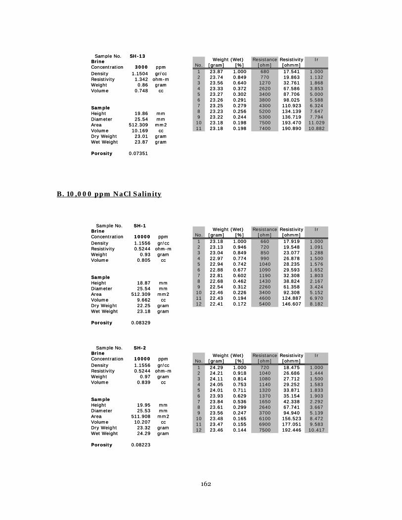
162

B. 10,000 ppm NaCl Salinity

Sample No. SH-13Brine Concentration 3000 ppmDensity 1.1504 gr/ccResistivity 1.342 ohm-mWeight 0.86 gramVolume 0.748 cc

SampleHeight 19.86 mmDiameter 25.54 mmArea 512.309 mm2Volume 10.169 ccDry Weight 23.01 gramWet Weight 23.87 gram

Porosity 0.07351

Resistance Resistivity IrNo. [gram] [%] [ohm] [ohmm]1 23.87 1.000 680 17.541 1.0002 23.74 0.849 770 19.863 1.1323 23.56 0.640 1270 32.761 1.8684 23.33 0.372 2620 67.586 3.8535 23.27 0.302 3400 87.706 5.0006 23.26 0.291 3800 98.025 5.5887 23.25 0.279 4300 110.923 6.3248 23.23 0.256 5200 134.139 7.6479 23.22 0.244 5300 136.719 7.79410 23.18 0.198 7500 193.470 11.02911 23.18 0.198 7400 190.890 10.882

Weight (Wet)Sample No. SH-13

Brine Concentration 3000 ppmDensity 1.1504 gr/ccResistivity 1.342 ohm-mWeight 0.86 gramVolume 0.748 cc

SampleHeight 19.86 mmDiameter 25.54 mmArea 512.309 mm2Volume 10.169 ccDry Weight 23.01 gramWet Weight 23.87 gram

Porosity 0.07351

Resistance Resistivity IrNo. [gram] [%] [ohm] [ohmm]1 23.87 1.000 680 17.541 1.0002 23.74 0.849 770 19.863 1.1323 23.56 0.640 1270 32.761 1.8684 23.33 0.372 2620 67.586 3.8535 23.27 0.302 3400 87.706 5.0006 23.26 0.291 3800 98.025 5.5887 23.25 0.279 4300 110.923 6.3248 23.23 0.256 5200 134.139 7.6479 23.22 0.244 5300 136.719 7.79410 23.18 0.198 7500 193.470 11.02911 23.18 0.198 7400 190.890 10.882

Weight (Wet)

Sample No. SH-1Brine Concentration 10000 ppmDensity 1.1556 gr/ccResistivity 0.5244 ohm-mWeight 0.93 gramVolume 0.805 cc

SampleHeight 18.87 mmDiameter 25.54 mmArea 512.309 mm2Volume 9.662 ccDry Weight 22.25 gramWet Weight 23.18 gram

Porosity 0.08329

Resistance Resistivity IrNo. [gram] [%] [ohm] [ohmm]1 23.18 1.000 660 17.919 1.0002 23.13 0.946 720 19.548 1.0913 23.04 0.849 850 23.077 1.2884 22.97 0.774 990 26.878 1.5005 22.94 0.742 1040 28.235 1.5766 22.88 0.677 1090 29.593 1.6527 22.81 0.602 1190 32.308 1.8038 22.68 0.462 1430 38.824 2.1679 22.54 0.312 2260 61.358 3.42410 22.46 0.226 3400 92.308 5.15211 22.43 0.194 4600 124.887 6.97012 22.41 0.172 5400 146.607 8.182

Weight (Wet)Sample No. SH-1

Brine Concentration 10000 ppmDensity 1.1556 gr/ccResistivity 0.5244 ohm-mWeight 0.93 gramVolume 0.805 cc

SampleHeight 18.87 mmDiameter 25.54 mmArea 512.309 mm2Volume 9.662 ccDry Weight 22.25 gramWet Weight 23.18 gram

Porosity 0.08329

Resistance Resistivity IrNo. [gram] [%] [ohm] [ohmm]1 23.18 1.000 660 17.919 1.0002 23.13 0.946 720 19.548 1.0913 23.04 0.849 850 23.077 1.2884 22.97 0.774 990 26.878 1.5005 22.94 0.742 1040 28.235 1.5766 22.88 0.677 1090 29.593 1.6527 22.81 0.602 1190 32.308 1.8038 22.68 0.462 1430 38.824 2.1679 22.54 0.312 2260 61.358 3.42410 22.46 0.226 3400 92.308 5.15211 22.43 0.194 4600 124.887 6.97012 22.41 0.172 5400 146.607 8.182

Weight (Wet)

Sample No. SH-2Brine Concentration 10000 ppmDensity 1.1556 gr/ccResistivity 0.5244 ohm-mWeight 0.97 gramVolume 0.839 cc

SampleHeight 19.95 mmDiameter 25.53 mmArea 511.908 mm2Volume 10.207 ccDry Weight 23.32 gramWet Weight 24.29 gram

Porosity 0.08223

Resistance Resistivity IrNo. [gram] [%] [ohm] [ohmm]1 24.29 1.000 720 18.475 1.0002 24.21 0.918 1040 26.686 1.4443 24.11 0.814 1080 27.712 1.5004 24.05 0.753 1140 29.252 1.5835 24.01 0.711 1320 33.871 1.8336 23.93 0.629 1370 35.154 1.9037 23.84 0.536 1650 42.338 2.2928 23.61 0.299 2640 67.741 3.6679 23.56 0.247 3700 94.940 5.13910 23.48 0.165 6100 156.523 8.47211 23.47 0.155 6900 177.051 9.58312 23.46 0.144 7500 192.446 10.417

Weight (Wet)

Sample No. SH-2Brine Concentration 10000 ppmDensity 1.1556 gr/ccResistivity 0.5244 ohm-mWeight 0.97 gramVolume 0.839 cc

SampleHeight 19.95 mmDiameter 25.53 mmArea 511.908 mm2Volume 10.207 ccDry Weight 23.32 gramWet Weight 24.29 gram

Porosity 0.08223

Resistance Resistivity IrNo. [gram] [%] [ohm] [ohmm]1 24.29 1.000 720 18.475 1.0002 24.21 0.918 1040 26.686 1.4443 24.11 0.814 1080 27.712 1.5004 24.05 0.753 1140 29.252 1.5835 24.01 0.711 1320 33.871 1.8336 23.93 0.629 1370 35.154 1.9037 23.84 0.536 1650 42.338 2.2928 23.61 0.299 2640 67.741 3.6679 23.56 0.247 3700 94.940 5.13910 23.48 0.165 6100 156.523 8.47211 23.47 0.155 6900 177.051 9.58312 23.46 0.144 7500 192.446 10.417

Weight (Wet)

163

Sample No. SH-3Brine Concentration 10000 ppmDensity 1.1556 gr/ccResistivity 0.5244 ohm-mWeight 0.93 gramVolume 0.805 cc

SampleHeight 18.87 mmDiameter 25.55 mmArea 512.710 mm2Volume 9.670 ccDry Weight 22.56 gramWet Weight 23.49 gram

Porosity 0.08322

Resistance Resistivity IrNo. [gram] [%] [ohm] [ohmm]1 23.49 1.000 660 17.933 1.0002 23.44 0.946 760 20.650 1.1523 23.35 0.849 840 22.823 1.2734 23.31 0.806 880 23.910 1.3335 23.21 0.699 1100 29.888 1.6676 23.04 0.516 1430 38.854 2.1677 22.97 0.441 1460 39.669 2.2128 22.81 0.269 2130 57.873 3.2279 22.72 0.172 4200 114.117 6.36410 22.68 0.129 5600 152.156 8.48511 22.68 0.129 6000 163.024 9.09112 22.68 0.129 5900 160.307 8.939

Weight (Wet)

Sample No. SH-3Brine Concentration 10000 ppmDensity 1.1556 gr/ccResistivity 0.5244 ohm-mWeight 0.93 gramVolume 0.805 cc

SampleHeight 18.87 mmDiameter 25.55 mmArea 512.710 mm2Volume 9.670 ccDry Weight 22.56 gramWet Weight 23.49 gram

Porosity 0.08322

Resistance Resistivity IrNo. [gram] [%] [ohm] [ohmm]1 23.49 1.000 660 17.933 1.0002 23.44 0.946 760 20.650 1.1523 23.35 0.849 840 22.823 1.2734 23.31 0.806 880 23.910 1.3335 23.21 0.699 1100 29.888 1.6676 23.04 0.516 1430 38.854 2.1677 22.97 0.441 1460 39.669 2.2128 22.81 0.269 2130 57.873 3.2279 22.72 0.172 4200 114.117 6.36410 22.68 0.129 5600 152.156 8.48511 22.68 0.129 6000 163.024 9.09112 22.68 0.129 5900 160.307 8.939

Weight (Wet)

Sample No. SH-4Brine Concentration 10000 ppmDensity 1.1556 gr/ccResistivity 0.5244 ohm-mWeight 0.84 gramVolume 0.727 cc

SampleHeight 17.75 mmDiameter 25.54 mmArea 512.309 mm2Volume 9.089 ccDry Weight 21.3 gramWet Weight 22.14 gram

Porosity 0.07998

Resistance Resistivity IrNo. [gram] [%] [ohm] [ohmm]1 22.14 1.000 640 18.472 1.0002 22.06 0.905 710 20.492 1.1093 21.83 0.631 1120 32.326 1.7504 21.82 0.619 1110 32.037 1.7345 21.81 0.607 1110 32.037 1.7346 21.76 0.548 1470 42.428 2.2977 21.68 0.452 1240 35.789 1.9388 21.48 0.214 2620 75.620 4.0949 21.45 0.179 3800 109.677 5.93810 21.42 0.143 4700 135.654 7.34411 21.41 0.131 5400 155.857 8.43812 21.41 0.131 5200 150.085 8.125

Weight (Wet)

Sample No. SH-4Brine Concentration 10000 ppmDensity 1.1556 gr/ccResistivity 0.5244 ohm-mWeight 0.84 gramVolume 0.727 cc

SampleHeight 17.75 mmDiameter 25.54 mmArea 512.309 mm2Volume 9.089 ccDry Weight 21.3 gramWet Weight 22.14 gram

Porosity 0.07998

Resistance Resistivity IrNo. [gram] [%] [ohm] [ohmm]1 22.14 1.000 640 18.472 1.0002 22.06 0.905 710 20.492 1.1093 21.83 0.631 1120 32.326 1.7504 21.82 0.619 1110 32.037 1.7345 21.81 0.607 1110 32.037 1.7346 21.76 0.548 1470 42.428 2.2977 21.68 0.452 1240 35.789 1.9388 21.48 0.214 2620 75.620 4.0949 21.45 0.179 3800 109.677 5.93810 21.42 0.143 4700 135.654 7.34411 21.41 0.131 5400 155.857 8.43812 21.41 0.131 5200 150.085 8.125

Weight (Wet)

Sample No. SH-5Brine Concentration 10000 ppmDensity 1.1556 gr/ccResistivity 0.5244 ohm-mWeight 0.81 gramVolume 0.701 cc

SampleHeight 18.85 mmDiameter 25.54 mmArea 512.309 mm2Volume 9.652 ccDry Weight 22.46 gramWet Weight 23.27 gram

Porosity 0.07262

Resistance Resistivity IrNo. [gram] [%] [ohm] [ohmm]1 23.27 1.000 860 23.373 1.0002 23.23 0.951 970 26.363 1.1283 23.17 0.877 1100 29.896 1.2794 23.13 0.827 1110 30.168 1.2915 23.05 0.728 1300 35.332 1.5126 22.95 0.605 1360 36.962 1.5817 22.90 0.543 1390 37.778 1.6168 22.74 0.346 1800 48.921 2.0939 22.66 0.247 2590 70.391 3.01210 22.59 0.160 4100 111.431 4.76711 22.58 0.148 4800 130.455 5.58112 22.57 0.136 5400 146.762 6.279

Weight (Wet)Sample No. SH-5

Brine Concentration 10000 ppmDensity 1.1556 gr/ccResistivity 0.5244 ohm-mWeight 0.81 gramVolume 0.701 cc

SampleHeight 18.85 mmDiameter 25.54 mmArea 512.309 mm2Volume 9.652 ccDry Weight 22.46 gramWet Weight 23.27 gram

Porosity 0.07262

Resistance Resistivity IrNo. [gram] [%] [ohm] [ohmm]1 23.27 1.000 860 23.373 1.0002 23.23 0.951 970 26.363 1.1283 23.17 0.877 1100 29.896 1.2794 23.13 0.827 1110 30.168 1.2915 23.05 0.728 1300 35.332 1.5126 22.95 0.605 1360 36.962 1.5817 22.90 0.543 1390 37.778 1.6168 22.74 0.346 1800 48.921 2.0939 22.66 0.247 2590 70.391 3.01210 22.59 0.160 4100 111.431 4.76711 22.58 0.148 4800 130.455 5.58112 22.57 0.136 5400 146.762 6.279

Weight (Wet)

164

Sample No. SH-6Brine Concentration 10000 ppmDensity 1.1556 gr/ccResistivity 0.5244 ohm-mWeight 0.73 gramVolume 0.632 cc

SampleHeight 16.65 mmDiameter 25.53 mmArea 511.908 mm2Volume 8.519 ccDry Weight 19.71 gramWet Weight 20.44 gram

Porosity 0.07415

Resistance Resistivity IrNo. [gram] [%] [ohm] [ohmm]1 20.44 1.000 770 23.674 1.0002 20.38 0.918 880 27.056 1.1433 20.26 0.753 1120 34.435 1.4554 20.25 0.740 1150 35.357 1.4945 20.23 0.712 1180 36.279 1.5326 20.18 0.644 1190 36.587 1.5457 20.13 0.575 1240 38.124 1.6108 19.99 0.384 1520 46.733 1.9749 19.89 0.247 2330 71.636 3.02610 19.83 0.164 3600 110.683 4.67511 19.81 0.137 4700 144.502 6.10412 19.80 0.123 5200 159.875 6.753

Weight (Wet)Sample No. SH-6

Brine Concentration 10000 ppmDensity 1.1556 gr/ccResistivity 0.5244 ohm-mWeight 0.73 gramVolume 0.632 cc

SampleHeight 16.65 mmDiameter 25.53 mmArea 511.908 mm2Volume 8.519 ccDry Weight 19.71 gramWet Weight 20.44 gram

Porosity 0.07415

Resistance Resistivity IrNo. [gram] [%] [ohm] [ohmm]1 20.44 1.000 770 23.674 1.0002 20.38 0.918 880 27.056 1.1433 20.26 0.753 1120 34.435 1.4554 20.25 0.740 1150 35.357 1.4945 20.23 0.712 1180 36.279 1.5326 20.18 0.644 1190 36.587 1.5457 20.13 0.575 1240 38.124 1.6108 19.99 0.384 1520 46.733 1.9749 19.89 0.247 2330 71.636 3.02610 19.83 0.164 3600 110.683 4.67511 19.81 0.137 4700 144.502 6.10412 19.80 0.123 5200 159.875 6.753

Weight (Wet)

Sample No. SH-7Brine Concentration 10000 ppmDensity 1.1556 gr/ccResistivity 0.5244 ohm-mWeight 0.77 gramVolume 0.666 cc

SampleHeight 17.77 mmDiameter 25.54 mmArea 512.309 mm2Volume 9.099 ccDry Weight 21.85 gramWet Weight 22.62 gram

Porosity 0.07323

Resistance Resistivity IrNo. [gram] [%] [ohm] [ohmm]1 22.62 1.000 510 14.703 1.0002 22.56 0.922 610 17.586 1.1963 22.48 0.818 740 21.334 1.4514 22.43 0.753 850 24.505 1.6675 22.39 0.701 1050 30.271 2.0596 22.31 0.597 1300 37.479 2.5497 22.30 0.584 1340 38.632 2.6278 22.22 0.481 1850 53.335 3.6279 22.16 0.403 2580 74.381 5.05910 22.06 0.273 4300 123.969 8.43111 22.05 0.260 4900 141.267 9.60812 22.03 0.234 5500 158.565 10.784

Weight (Wet)

Sample No. SH-7Brine Concentration 10000 ppmDensity 1.1556 gr/ccResistivity 0.5244 ohm-mWeight 0.77 gramVolume 0.666 cc

SampleHeight 17.77 mmDiameter 25.54 mmArea 512.309 mm2Volume 9.099 ccDry Weight 21.85 gramWet Weight 22.62 gram

Porosity 0.07323

Resistance Resistivity IrNo. [gram] [%] [ohm] [ohmm]1 22.62 1.000 510 14.703 1.0002 22.56 0.922 610 17.586 1.1963 22.48 0.818 740 21.334 1.4514 22.43 0.753 850 24.505 1.6675 22.39 0.701 1050 30.271 2.0596 22.31 0.597 1300 37.479 2.5497 22.30 0.584 1340 38.632 2.6278 22.22 0.481 1850 53.335 3.6279 22.16 0.403 2580 74.381 5.05910 22.06 0.273 4300 123.969 8.43111 22.05 0.260 4900 141.267 9.60812 22.03 0.234 5500 158.565 10.784

Weight (Wet)

Sample No. SH-8Brine Concentration 10000 ppmDensity 1.1556 gr/ccResistivity 0.5244 ohm-mWeight 0.79 gramVolume 0.684 cc

SampleHeight 18.32 mmDiameter 25.52 mmArea 511.507 mm2Volume 9.366 ccDry Weight 22.66 gramWet Weight 23.45 gram

Porosity 0.07299

Resistance Resistivity IrNo. [gram] [%] [ohm] [ohmm]1 23.45 1.000 570 15.915 1.0002 23.39 0.924 670 18.707 1.1753 23.30 0.810 780 21.778 1.3684 23.22 0.709 1020 28.479 1.7895 23.17 0.646 1170 32.667 2.0536 23.14 0.608 1200 33.505 2.1057 23.13 0.595 1210 33.784 2.1238 23.04 0.481 1490 41.602 2.6149 22.94 0.354 2230 62.263 3.91210 22.88 0.278 3040 84.879 5.33311 22.85 0.241 3800 106.099 6.66712 22.84 0.228 4000 111.683 7.018

Weight (Wet)

Sample No. SH-8Brine Concentration 10000 ppmDensity 1.1556 gr/ccResistivity 0.5244 ohm-mWeight 0.79 gramVolume 0.684 cc

SampleHeight 18.32 mmDiameter 25.52 mmArea 511.507 mm2Volume 9.366 ccDry Weight 22.66 gramWet Weight 23.45 gram

Porosity 0.07299

Resistance Resistivity IrNo. [gram] [%] [ohm] [ohmm]1 23.45 1.000 570 15.915 1.0002 23.39 0.924 670 18.707 1.1753 23.30 0.810 780 21.778 1.3684 23.22 0.709 1020 28.479 1.7895 23.17 0.646 1170 32.667 2.0536 23.14 0.608 1200 33.505 2.1057 23.13 0.595 1210 33.784 2.1238 23.04 0.481 1490 41.602 2.6149 22.94 0.354 2230 62.263 3.91210 22.88 0.278 3040 84.879 5.33311 22.85 0.241 3800 106.099 6.66712 22.84 0.228 4000 111.683 7.018

Weight (Wet)

165

C. 20,000 ppm NaCl Salinity

Sample No. SH-10Brine Concentration 10000 ppmDensity 1.1556 gr/ccResistivity 0.5244 ohm-mWeight 0.81 gramVolume 0.701 cc

SampleHeight 18.28 mmDiameter 25.53 mmArea 511.908 mm2Volume 9.353 ccDry Weight 21.9 gramWet Weight 22.71 gram

Porosity 0.07494

Resistance Resistivity IrNo. [gram] [%] [ohm] [ohmm]1 22.71 1.000 460 12.882 1.0002 22.65 0.926 560 15.682 1.2173 22.56 0.815 830 23.243 1.8044 22.44 0.667 1150 32.204 2.5005 22.43 0.654 1160 32.484 2.5226 22.41 0.630 1250 35.005 2.7177 22.39 0.605 1270 35.565 2.7618 22.35 0.556 1460 40.885 3.1749 22.26 0.444 2090 58.528 4.54310 22.18 0.346 2740 76.730 5.95711 22.15 0.309 3230 90.452 7.02212 22.14 0.296 3500 98.013 7.609

Weight (Wet)

Sample No. SH-10Brine Concentration 10000 ppmDensity 1.1556 gr/ccResistivity 0.5244 ohm-mWeight 0.81 gramVolume 0.701 cc

SampleHeight 18.28 mmDiameter 25.53 mmArea 511.908 mm2Volume 9.353 ccDry Weight 21.9 gramWet Weight 22.71 gram

Porosity 0.07494

Resistance Resistivity IrNo. [gram] [%] [ohm] [ohmm]1 22.71 1.000 460 12.882 1.0002 22.65 0.926 560 15.682 1.2173 22.56 0.815 830 23.243 1.8044 22.44 0.667 1150 32.204 2.5005 22.43 0.654 1160 32.484 2.5226 22.41 0.630 1250 35.005 2.7177 22.39 0.605 1270 35.565 2.7618 22.35 0.556 1460 40.885 3.1749 22.26 0.444 2090 58.528 4.54310 22.18 0.346 2740 76.730 5.95711 22.15 0.309 3230 90.452 7.02212 22.14 0.296 3500 98.013 7.609

Weight (Wet)

Sample No. SH-11Brine Concentration 10000 ppmDensity 1.1556 gr/ccResistivity 0.5244 ohm-mWeight 0.76 gramVolume 0.658 cc

SampleHeight 18.29 mmDiameter 25.53 mmArea 511.908 mm2Volume 9.358 ccDry Weight 22.27 gramWet Weight 23.03 gram

Porosity 0.07028

Resistance Resistivity IrNo. [gram] [%] [ohm] [ohmm]1 23.03 1.000 1190 33.306 1.0002 22.96 0.908 1060 29.668 0.8913 22.82 0.724 1720 48.140 1.4454 22.80 0.697 1810 50.659 1.5215 22.76 0.645 1940 54.297 1.6306 22.73 0.605 1980 55.417 1.6647 22.71 0.579 2020 56.537 1.6978 22.61 0.447 1820 50.939 1.5299 22.57 0.395 3220 90.123 2.70610 22.46 0.250 4800 134.344 4.03411 22.45 0.237 4200 117.551 3.52912 22.44 0.224 4600 128.747 3.866

Weight (Wet)Sample No. SH-11

Brine Concentration 10000 ppmDensity 1.1556 gr/ccResistivity 0.5244 ohm-mWeight 0.76 gramVolume 0.658 cc

SampleHeight 18.29 mmDiameter 25.53 mmArea 511.908 mm2Volume 9.358 ccDry Weight 22.27 gramWet Weight 23.03 gram

Porosity 0.07028

Resistance Resistivity IrNo. [gram] [%] [ohm] [ohmm]1 23.03 1.000 1190 33.306 1.0002 22.96 0.908 1060 29.668 0.8913 22.82 0.724 1720 48.140 1.4454 22.80 0.697 1810 50.659 1.5215 22.76 0.645 1940 54.297 1.6306 22.73 0.605 1980 55.417 1.6647 22.71 0.579 2020 56.537 1.6978 22.61 0.447 1820 50.939 1.5299 22.57 0.395 3220 90.123 2.70610 22.46 0.250 4800 134.344 4.03411 22.45 0.237 4200 117.551 3.52912 22.44 0.224 4600 128.747 3.866

Weight (Wet)

Sample No. SH-1Brine Concentration 20000 ppmDensity 1.1636 gr/ccResistivity 0.278 ohm-mWeight 0.98 gramVolume 0.842 cc

SampleHeight 18.87 mmDiameter 25.54 mmArea 512.309 mm2Volume 9.662 ccDry Weight 22.17 gramWet Weight 23.15 gram

Porosity 0.08716

Resistance Resistivity IrNo. [gram] [%] [ohm] [ohmm]1 23.15 1.000 490 13.303 1.0002 23.09 0.939 580 15.747 1.1843 23.04 0.888 620 16.833 1.2654 23.01 0.857 660 17.919 1.3475 22.97 0.816 760 20.634 1.5516 22.92 0.765 880 23.891 1.7967 22.74 0.582 1240 33.665 2.5318 22.59 0.429 1650 44.796 3.3679 22.54 0.378 1910 51.855 3.89810 22.53 0.367 1920 52.127 3.91811 22.51 0.347 1990 54.027 4.06112 22.44 0.276 2620 71.131 5.34713 22.31 0.143 8800 238.914 17.95914 22.30 0.133 9500 257.919 19.388

Weight (Wet)Sample No. SH-1

Brine Concentration 20000 ppmDensity 1.1636 gr/ccResistivity 0.278 ohm-mWeight 0.98 gramVolume 0.842 cc

SampleHeight 18.87 mmDiameter 25.54 mmArea 512.309 mm2Volume 9.662 ccDry Weight 22.17 gramWet Weight 23.15 gram

Porosity 0.08716

Resistance Resistivity IrNo. [gram] [%] [ohm] [ohmm]1 23.15 1.000 490 13.303 1.0002 23.09 0.939 580 15.747 1.1843 23.04 0.888 620 16.833 1.2654 23.01 0.857 660 17.919 1.3475 22.97 0.816 760 20.634 1.5516 22.92 0.765 880 23.891 1.7967 22.74 0.582 1240 33.665 2.5318 22.59 0.429 1650 44.796 3.3679 22.54 0.378 1910 51.855 3.89810 22.53 0.367 1920 52.127 3.91811 22.51 0.347 1990 54.027 4.06112 22.44 0.276 2620 71.131 5.34713 22.31 0.143 8800 238.914 17.95914 22.30 0.133 9500 257.919 19.388

Weight (Wet)

166

Sample No. SH-1Brine Concentration 20000 ppmDensity 1.1636 gr/ccResistivity 0.278 ohm-mWeight 0.98 gramVolume 0.842 cc

SampleHeight 18.87 mmDiameter 25.54 mmArea 512.309 mm2Volume 9.662 ccDry Weight 22.17 gramWet Weight 23.15 gram

Porosity 0.08716

Resistance Resistivity IrNo. [gram] [%] [ohm] [ohmm]1 23.15 1.000 490 13.303 1.0002 23.09 0.939 580 15.747 1.1843 23.04 0.888 620 16.833 1.2654 23.01 0.857 660 17.919 1.3475 22.97 0.816 760 20.634 1.5516 22.92 0.765 880 23.891 1.7967 22.74 0.582 1240 33.665 2.5318 22.59 0.429 1650 44.796 3.3679 22.54 0.378 1910 51.855 3.89810 22.53 0.367 1920 52.127 3.91811 22.51 0.347 1990 54.027 4.06112 22.44 0.276 2620 71.131 5.34713 22.31 0.143 8800 238.914 17.95914 22.30 0.133 9500 257.919 19.388

Weight (Wet)Sample No. SH-1

Brine Concentration 20000 ppmDensity 1.1636 gr/ccResistivity 0.278 ohm-mWeight 0.98 gramVolume 0.842 cc

SampleHeight 18.87 mmDiameter 25.54 mmArea 512.309 mm2Volume 9.662 ccDry Weight 22.17 gramWet Weight 23.15 gram

Porosity 0.08716

Resistance Resistivity IrNo. [gram] [%] [ohm] [ohmm]1 23.15 1.000 490 13.303 1.0002 23.09 0.939 580 15.747 1.1843 23.04 0.888 620 16.833 1.2654 23.01 0.857 660 17.919 1.3475 22.97 0.816 760 20.634 1.5516 22.92 0.765 880 23.891 1.7967 22.74 0.582 1240 33.665 2.5318 22.59 0.429 1650 44.796 3.3679 22.54 0.378 1910 51.855 3.89810 22.53 0.367 1920 52.127 3.91811 22.51 0.347 1990 54.027 4.06112 22.44 0.276 2620 71.131 5.34713 22.31 0.143 8800 238.914 17.95914 22.30 0.133 9500 257.919 19.388

Weight (Wet)

Sample No. SH-2Brine Concentration 20000 ppmDensity 1.1636 gr/ccResistivity 0.278 ohm-mWeight 1.04 gramVolume 0.894 cc

SampleHeight 19.95 mmDiameter 25.53 mmArea 511.908 mm2Volume 10.207 ccDry Weight 23.26 gramWet Weight 24.3 gram

Porosity 0.08756

Resistance Resistivity IrNo. [gram] [%] [ohm] [ohmm]1 24.30 1.000 470 12.060 1.0002 24.24 0.942 570 14.626 1.2133 24.20 0.904 600 15.396 1.2774 24.15 0.856 660 16.935 1.4045 24.07 0.779 810 20.784 1.7236 23.99 0.702 980 25.146 2.0857 23.86 0.577 1220 31.305 2.5968 23.74 0.462 1430 36.693 3.0439 23.70 0.423 1580 40.542 3.36210 23.65 0.375 1830 46.957 3.89411 23.61 0.337 1890 48.497 4.02112 23.54 0.269 2930 75.182 6.23413 23.39 0.125 13100 336.140 27.87214 23.38 0.115 13600 348.970 28.936

Weight (Wet)

Sample No. SH-2Brine Concentration 20000 ppmDensity 1.1636 gr/ccResistivity 0.278 ohm-mWeight 1.04 gramVolume 0.894 cc

SampleHeight 19.95 mmDiameter 25.53 mmArea 511.908 mm2Volume 10.207 ccDry Weight 23.26 gramWet Weight 24.3 gram

Porosity 0.08756

Resistance Resistivity IrNo. [gram] [%] [ohm] [ohmm]1 24.30 1.000 470 12.060 1.0002 24.24 0.942 570 14.626 1.2133 24.20 0.904 600 15.396 1.2774 24.15 0.856 660 16.935 1.4045 24.07 0.779 810 20.784 1.7236 23.99 0.702 980 25.146 2.0857 23.86 0.577 1220 31.305 2.5968 23.74 0.462 1430 36.693 3.0439 23.70 0.423 1580 40.542 3.36210 23.65 0.375 1830 46.957 3.89411 23.61 0.337 1890 48.497 4.02112 23.54 0.269 2930 75.182 6.23413 23.39 0.125 13100 336.140 27.87214 23.38 0.115 13600 348.970 28.936

Weight (Wet)

Sample No. SH-3Brine Concentration 20000 ppmDensity 1.1636 gr/ccResistivity 0.278 ohm-mWeight 1 gramVolume 0.859 cc

SampleHeight 18.87 mmDiameter 25.55 mmArea 512.710 mm2Volume 9.670 ccDry Weight 22.52 gramWet Weight 23.52 gram

Porosity 0.08887

Resistance Resistivity IrNo. [gram] [%] [ohm] [ohmm]1 23.52 1.000 440 11.955 1.0002 23.47 0.950 530 14.400 1.2053 23.39 0.870 580 15.759 1.3184 23.34 0.820 640 17.389 1.4555 23.28 0.760 750 20.378 1.7056 23.18 0.660 910 24.725 2.0687 23.08 0.560 1060 28.801 2.4098 22.96 0.440 1250 33.963 2.8419 22.89 0.370 1510 41.028 3.43210 22.88 0.360 1520 41.299 3.45511 22.87 0.350 1530 41.571 3.47712 22.82 0.300 1770 48.092 4.02313 22.69 0.170 4900 133.136 11.13614 22.68 0.160 5600 152.156 12.727

Weight (Wet)Sample No. SH-3

Brine Concentration 20000 ppmDensity 1.1636 gr/ccResistivity 0.278 ohm-mWeight 1 gramVolume 0.859 cc

SampleHeight 18.87 mmDiameter 25.55 mmArea 512.710 mm2Volume 9.670 ccDry Weight 22.52 gramWet Weight 23.52 gram

Porosity 0.08887

Resistance Resistivity IrNo. [gram] [%] [ohm] [ohmm]1 23.52 1.000 440 11.955 1.0002 23.47 0.950 530 14.400 1.2053 23.39 0.870 580 15.759 1.3184 23.34 0.820 640 17.389 1.4555 23.28 0.760 750 20.378 1.7056 23.18 0.660 910 24.725 2.0687 23.08 0.560 1060 28.801 2.4098 22.96 0.440 1250 33.963 2.8419 22.89 0.370 1510 41.028 3.43210 22.88 0.360 1520 41.299 3.45511 22.87 0.350 1530 41.571 3.47712 22.82 0.300 1770 48.092 4.02313 22.69 0.170 4900 133.136 11.13614 22.68 0.160 5600 152.156 12.727

Weight (Wet)

167

Sample No. SH-4Brine Concentration 20000 ppmDensity 1.1636 gr/ccResistivity 0.278 ohm-mWeight 0.91 gramVolume 0.782 cc

SampleHeight 17.75 mmDiameter 25.54 mmArea 512.309 mm2Volume 9.089 ccDry Weight 21.24 gramWet Weight 22.15 gram

Porosity 0.08605

Resistance Resistivity IrNo. [gram] [%] [ohm] [ohmm]1 22.15 1.000 450 12.988 1.0002 22.10 0.945 510 14.720 1.1333 22.04 0.879 550 15.874 1.2224 22.01 0.846 590 17.029 1.3115 21.95 0.780 690 19.915 1.5336 21.90 0.725 780 22.513 1.7337 21.81 0.626 910 26.265 2.0228 21.70 0.505 1050 30.306 2.3339 21.62 0.418 1270 36.655 2.82210 21.59 0.385 1380 39.830 3.06711 21.52 0.308 2160 62.343 4.80012 21.46 0.242 5700 164.516 12.66713 21.37 0.143 6600 190.492 14.66714 21.36 0.132 8400 242.445 18.667

Weight (Wet)Sample No. SH-4

Brine Concentration 20000 ppmDensity 1.1636 gr/ccResistivity 0.278 ohm-mWeight 0.91 gramVolume 0.782 cc

SampleHeight 17.75 mmDiameter 25.54 mmArea 512.309 mm2Volume 9.089 ccDry Weight 21.24 gramWet Weight 22.15 gram

Porosity 0.08605

Resistance Resistivity IrNo. [gram] [%] [ohm] [ohmm]1 22.15 1.000 450 12.988 1.0002 22.10 0.945 510 14.720 1.1333 22.04 0.879 550 15.874 1.2224 22.01 0.846 590 17.029 1.3115 21.95 0.780 690 19.915 1.5336 21.90 0.725 780 22.513 1.7337 21.81 0.626 910 26.265 2.0228 21.70 0.505 1050 30.306 2.3339 21.62 0.418 1270 36.655 2.82210 21.59 0.385 1380 39.830 3.06711 21.52 0.308 2160 62.343 4.80012 21.46 0.242 5700 164.516 12.66713 21.37 0.143 6600 190.492 14.66714 21.36 0.132 8400 242.445 18.667

Weight (Wet)

Sample No. SH-5Brine Concentration 20000 ppmDensity 1.1636 gr/ccResistivity 0.278 ohm-mWeight 0.89 gramVolume 0.765 cc

SampleHeight 18.85 mmDiameter 25.54 mmArea 512.309 mm2Volume 9.652 ccDry Weight 22.4 gramWet Weight 23.29 gram

Porosity 0.07924

Resistance Resistivity IrNo. [gram] [%] [ohm] [ohmm]1 23.29 1.000 620 16.850 1.0002 23.23 0.933 730 19.840 1.1773 23.20 0.899 760 20.655 1.2264 23.17 0.865 810 22.014 1.3065 23.11 0.798 930 25.276 1.5006 23.03 0.708 1050 28.537 1.6947 22.95 0.618 1210 32.886 1.9528 22.84 0.494 1330 36.147 2.1459 22.75 0.393 1630 44.300 2.62910 22.72 0.360 1760 47.834 2.83911 22.70 0.337 1900 51.639 3.06512 22.62 0.247 2630 71.479 4.24213 22.53 0.146 7300 198.401 11.77414 22.52 0.135 9000 244.604 14.516

Weight (Wet)

Sample No. SH-5Brine Concentration 20000 ppmDensity 1.1636 gr/ccResistivity 0.278 ohm-mWeight 0.89 gramVolume 0.765 cc

SampleHeight 18.85 mmDiameter 25.54 mmArea 512.309 mm2Volume 9.652 ccDry Weight 22.4 gramWet Weight 23.29 gram

Porosity 0.07924

Resistance Resistivity IrNo. [gram] [%] [ohm] [ohmm]1 23.29 1.000 620 16.850 1.0002 23.23 0.933 730 19.840 1.1773 23.20 0.899 760 20.655 1.2264 23.17 0.865 810 22.014 1.3065 23.11 0.798 930 25.276 1.5006 23.03 0.708 1050 28.537 1.6947 22.95 0.618 1210 32.886 1.9528 22.84 0.494 1330 36.147 2.1459 22.75 0.393 1630 44.300 2.62910 22.72 0.360 1760 47.834 2.83911 22.70 0.337 1900 51.639 3.06512 22.62 0.247 2630 71.479 4.24213 22.53 0.146 7300 198.401 11.77414 22.52 0.135 9000 244.604 14.516

Weight (Wet)

Sample No. SH-6Brine Concentration 20000 ppmDensity 1.1636 gr/ccResistivity 0.278 ohm-mWeight 0.78 gramVolume 0.670 cc

SampleHeight 16.65 mmDiameter 25.53 mmArea 511.908 mm2Volume 8.519 ccDry Weight 19.68 gramWet Weight 20.46 gram

Porosity 0.07869

Resistance Resistivity IrNo. [gram] [%] [ohm] [ohmm]1 20.46 1.000 520 15.988 1.0002 20.40 0.923 650 19.984 1.2503 20.37 0.885 690 21.214 1.3274 20.32 0.821 810 24.904 1.5585 20.25 0.731 910 27.978 1.7506 20.20 0.667 1010 31.053 1.9427 20.03 0.449 1350 41.506 2.5968 19.96 0.359 1660 51.037 3.1929 19.94 0.333 1750 53.804 3.36510 19.93 0.321 1850 56.879 3.55811 19.89 0.269 2210 67.947 4.25012 19.82 0.179 3500 107.608 6.73113 19.77 0.115 6200 190.620 11.92314 19.76 0.103 7400 227.514 14.231

Weight (Wet)Sample No. SH-6

Brine Concentration 20000 ppmDensity 1.1636 gr/ccResistivity 0.278 ohm-mWeight 0.78 gramVolume 0.670 cc

SampleHeight 16.65 mmDiameter 25.53 mmArea 511.908 mm2Volume 8.519 ccDry Weight 19.68 gramWet Weight 20.46 gram

Porosity 0.07869

Resistance Resistivity IrNo. [gram] [%] [ohm] [ohmm]1 20.46 1.000 520 15.988 1.0002 20.40 0.923 650 19.984 1.2503 20.37 0.885 690 21.214 1.3274 20.32 0.821 810 24.904 1.5585 20.25 0.731 910 27.978 1.7506 20.20 0.667 1010 31.053 1.9427 20.03 0.449 1350 41.506 2.5968 19.96 0.359 1660 51.037 3.1929 19.94 0.333 1750 53.804 3.36510 19.93 0.321 1850 56.879 3.55811 19.89 0.269 2210 67.947 4.25012 19.82 0.179 3500 107.608 6.73113 19.77 0.115 6200 190.620 11.92314 19.76 0.103 7400 227.514 14.231

Weight (Wet)

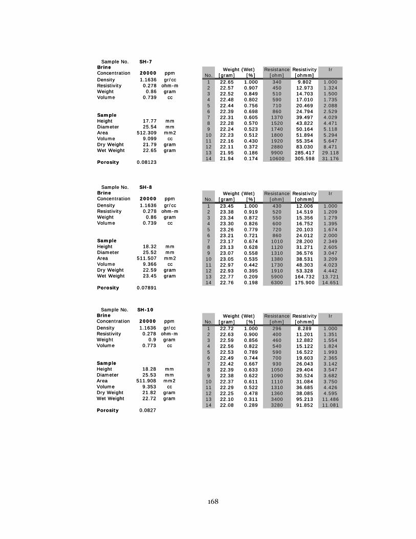
168

Sample No. SH-7Brine Concentration 20000 ppmDensity 1.1636 gr/ccResistivity 0.278 ohm-mWeight 0.86 gramVolume 0.739 cc

SampleHeight 17.77 mmDiameter 25.54 mmArea 512.309 mm2Volume 9.099 ccDry Weight 21.79 gramWet Weight 22.65 gram

Porosity 0.08123

Resistance Resistivity IrNo. [gram] [%] [ohm] [ohmm]1 22.65 1.000 340 9.802 1.0002 22.57 0.907 450 12.973 1.3243 22.52 0.849 510 14.703 1.5004 22.48 0.802 590 17.010 1.7355 22.44 0.756 710 20.469 2.0886 22.39 0.698 860 24.794 2.5297 22.31 0.605 1370 39.497 4.0298 22.28 0.570 1520 43.822 4.4719 22.24 0.523 1740 50.164 5.11810 22.23 0.512 1800 51.894 5.29411 22.16 0.430 1920 55.354 5.64712 22.11 0.372 2880 83.030 8.47113 21.95 0.186 9900 285.417 29.11814 21.94 0.174 10600 305.598 31.176

Weight (Wet)

Sample No. SH-7Brine Concentration 20000 ppmDensity 1.1636 gr/ccResistivity 0.278 ohm-mWeight 0.86 gramVolume 0.739 cc

SampleHeight 17.77 mmDiameter 25.54 mmArea 512.309 mm2Volume 9.099 ccDry Weight 21.79 gramWet Weight 22.65 gram

Porosity 0.08123

Resistance Resistivity IrNo. [gram] [%] [ohm] [ohmm]1 22.65 1.000 340 9.802 1.0002 22.57 0.907 450 12.973 1.3243 22.52 0.849 510 14.703 1.5004 22.48 0.802 590 17.010 1.7355 22.44 0.756 710 20.469 2.0886 22.39 0.698 860 24.794 2.5297 22.31 0.605 1370 39.497 4.0298 22.28 0.570 1520 43.822 4.4719 22.24 0.523 1740 50.164 5.11810 22.23 0.512 1800 51.894 5.29411 22.16 0.430 1920 55.354 5.64712 22.11 0.372 2880 83.030 8.47113 21.95 0.186 9900 285.417 29.11814 21.94 0.174 10600 305.598 31.176

Weight (Wet)

Sample No. SH-8Brine Concentration 20000 ppmDensity 1.1636 gr/ccResistivity 0.278 ohm-mWeight 0.86 gramVolume 0.739 cc

SampleHeight 18.32 mmDiameter 25.52 mmArea 511.507 mm2Volume 9.366 ccDry Weight 22.59 gramWet Weight 23.45 gram

Porosity 0.07891

Resistance Resistivity IrNo. [gram] [%] [ohm] [ohmm]1 23.45 1.000 430 12.006 1.0002 23.38 0.919 520 14.519 1.2093 23.34 0.872 550 15.356 1.2794 23.30 0.826 600 16.752 1.3955 23.26 0.779 720 20.103 1.6746 23.21 0.721 860 24.012 2.0007 23.17 0.674 1010 28.200 2.3498 23.13 0.628 1120 31.271 2.6059 23.07 0.558 1310 36.576 3.04710 23.05 0.535 1380 38.531 3.20911 22.97 0.442 1730 48.303 4.02312 22.93 0.395 1910 53.328 4.44213 22.77 0.209 5900 164.732 13.72114 22.76 0.198 6300 175.900 14.651

Weight (Wet)Sample No. SH-8

Brine Concentration 20000 ppmDensity 1.1636 gr/ccResistivity 0.278 ohm-mWeight 0.86 gramVolume 0.739 cc

SampleHeight 18.32 mmDiameter 25.52 mmArea 511.507 mm2Volume 9.366 ccDry Weight 22.59 gramWet Weight 23.45 gram

Porosity 0.07891

Resistance Resistivity IrNo. [gram] [%] [ohm] [ohmm]1 23.45 1.000 430 12.006 1.0002 23.38 0.919 520 14.519 1.2093 23.34 0.872 550 15.356 1.2794 23.30 0.826 600 16.752 1.3955 23.26 0.779 720 20.103 1.6746 23.21 0.721 860 24.012 2.0007 23.17 0.674 1010 28.200 2.3498 23.13 0.628 1120 31.271 2.6059 23.07 0.558 1310 36.576 3.04710 23.05 0.535 1380 38.531 3.20911 22.97 0.442 1730 48.303 4.02312 22.93 0.395 1910 53.328 4.44213 22.77 0.209 5900 164.732 13.72114 22.76 0.198 6300 175.900 14.651

Weight (Wet)

Sample No. SH-10Brine Concentration 20000 ppmDensity 1.1636 gr/ccResistivity 0.278 ohm-mWeight 0.9 gramVolume 0.773 cc

SampleHeight 18.28 mmDiameter 25.53 mmArea 511.908 mm2Volume 9.353 ccDry Weight 21.82 gramWet Weight 22.72 gram

Porosity 0.0827

Resistance Resistivity IrNo. [gram] [%] [ohm] [ohmm]1 22.72 1.000 296 8.289 1.0002 22.63 0.900 400 11.201 1.3513 22.59 0.856 460 12.882 1.5544 22.56 0.822 540 15.122 1.8245 22.53 0.789 590 16.522 1.9936 22.49 0.744 700 19.603 2.3657 22.42 0.667 930 26.043 3.1428 22.39 0.633 1050 29.404 3.5479 22.38 0.622 1090 30.524 3.68210 22.37 0.611 1110 31.084 3.75011 22.29 0.522 1310 36.685 4.42612 22.25 0.478 1360 38.085 4.59513 22.10 0.311 3400 95.213 11.48614 22.08 0.289 3280 91.852 11.081

Weight (Wet)Sample No. SH-10

Brine Concentration 20000 ppmDensity 1.1636 gr/ccResistivity 0.278 ohm-mWeight 0.9 gramVolume 0.773 cc

SampleHeight 18.28 mmDiameter 25.53 mmArea 511.908 mm2Volume 9.353 ccDry Weight 21.82 gramWet Weight 22.72 gram

Porosity 0.0827

Resistance Resistivity IrNo. [gram] [%] [ohm] [ohmm]1 22.72 1.000 296 8.289 1.0002 22.63 0.900 400 11.201 1.3513 22.59 0.856 460 12.882 1.5544 22.56 0.822 540 15.122 1.8245 22.53 0.789 590 16.522 1.9936 22.49 0.744 700 19.603 2.3657 22.42 0.667 930 26.043 3.1428 22.39 0.633 1050 29.404 3.5479 22.38 0.622 1090 30.524 3.68210 22.37 0.611 1110 31.084 3.75011 22.29 0.522 1310 36.685 4.42612 22.25 0.478 1360 38.085 4.59513 22.10 0.311 3400 95.213 11.48614 22.08 0.289 3280 91.852 11.081

Weight (Wet)

169

D. 30,000 ppm NaCl Salinity

Sample No. SH-11Brine Concentration 20000 ppmDensity 1.1636 gr/ccResistivity 0.278 ohm-mWeight 0.85 gramVolume 0.730 cc

SampleHeight 18.29 mmDiameter 25.53 mmArea 511.908 mm2Volume 9.358 ccDry Weight 22.19 gramWet Weight 23.04 gram

Porosity 0.07806

Resistance Resistivity IrNo. [gram] [%] [ohm] [ohmm]1 23.04 1.000 400 11.195 1.0002 22.98 0.929 480 13.434 1.2003 22.94 0.882 510 14.274 1.2754 22.88 0.812 690 19.312 1.7255 22.84 0.765 690 19.312 1.7256 22.78 0.694 870 24.350 2.1757 22.68 0.576 1230 34.426 3.0758 22.62 0.506 1380 38.624 3.4509 22.61 0.494 1430 40.023 3.57510 22.60 0.482 1430 40.023 3.57511 22.55 0.424 1600 44.781 4.00012 22.45 0.306 2510 70.251 6.27513 22.30 0.129 11000 307.872 27.50014 22.30 0.129 10200 285.482 25.500

Weight (Wet)Sample No. SH-11

Brine Concentration 20000 ppmDensity 1.1636 gr/ccResistivity 0.278 ohm-mWeight 0.85 gramVolume 0.730 cc

SampleHeight 18.29 mmDiameter 25.53 mmArea 511.908 mm2Volume 9.358 ccDry Weight 22.19 gramWet Weight 23.04 gram

Porosity 0.07806

Resistance Resistivity IrNo. [gram] [%] [ohm] [ohmm]1 23.04 1.000 400 11.195 1.0002 22.98 0.929 480 13.434 1.2003 22.94 0.882 510 14.274 1.2754 22.88 0.812 690 19.312 1.7255 22.84 0.765 690 19.312 1.7256 22.78 0.694 870 24.350 2.1757 22.68 0.576 1230 34.426 3.0758 22.62 0.506 1380 38.624 3.4509 22.61 0.494 1430 40.023 3.57510 22.60 0.482 1430 40.023 3.57511 22.55 0.424 1600 44.781 4.00012 22.45 0.306 2510 70.251 6.27513 22.30 0.129 11000 307.872 27.50014 22.30 0.129 10200 285.482 25.500

Weight (Wet)

Resistance Resistivity IrNo. [gram] [%] [ohm] [ohmm]1 23.19 1.000 460 12.489 1.0002 23.12 0.927 510 13.846 1.1093 23.01 0.813 660 17.919 1.4354 22.84 0.635 950 25.792 2.0655 22.50 0.281 2500 67.873 5.4356 22.37 0.146 6500 176.471 14.1307 22.35 0.125 8400 228.055 18.261

Weight (Wet)

Sample No. SH-1Brine Concentration 30000 ppmDensity 1.1728 gr/ccResistivity 0.1962 ohm-mWeight 0.96 gramVolume 0.819 cc

SampleHeight 18.87 mmDiameter 25.54 mmArea 512.309 mm2Volume 9.662 ccDry Weight 22.23 gramWet Weight 23.19 gram

Porosity 0.08472

Resistance Resistivity IrNo. [gram] [%] [ohm] [ohmm]1 23.19 1.000 460 12.489 1.0002 23.12 0.927 510 13.846 1.1093 23.01 0.813 660 17.919 1.4354 22.84 0.635 950 25.792 2.0655 22.50 0.281 2500 67.873 5.4356 22.37 0.146 6500 176.471 14.1307 22.35 0.125 8400 228.055 18.261

Weight (Wet)

Sample No. SH-1Brine Concentration 30000 ppmDensity 1.1728 gr/ccResistivity 0.1962 ohm-mWeight 0.96 gramVolume 0.819 cc

SampleHeight 18.87 mmDiameter 25.54 mmArea 512.309 mm2Volume 9.662 ccDry Weight 22.23 gramWet Weight 23.19 gram

Porosity 0.08472

Resistance Resistivity IrNo. [gram] [%] [ohm] [ohmm]1 24.35 1.000 420 10.777 1.0002 24.21 0.859 590 15.139 1.4053 24.12 0.768 740 18.988 1.7624 23.83 0.475 1220 31.305 2.9055 23.61 0.253 2750 70.564 6.5486 23.49 0.131 7100 182.183 16.9057 23.47 0.111 8500 218.106 20.238

Weight (Wet)Sample No. SH-2Brine Concentration 30000 ppmDensity 1.1728 gr/ccResistivity 0.1962 ohm-mWeight 0.99 gramVolume 0.844 cc

SampleHeight 19.95 mmDiameter 25.53 mmArea 511.908 mm2Volume 10.207 ccDry Weight 23.36 gramWet Weight 24.35 gram

Porosity 0.0827

Resistance Resistivity IrNo. [gram] [%] [ohm] [ohmm]1 24.35 1.000 420 10.777 1.0002 24.21 0.859 590 15.139 1.4053 24.12 0.768 740 18.988 1.7624 23.83 0.475 1220 31.305 2.9055 23.61 0.253 2750 70.564 6.5486 23.49 0.131 7100 182.183 16.9057 23.47 0.111 8500 218.106 20.238

Weight (Wet)Sample No. SH-2Brine Concentration 30000 ppmDensity 1.1728 gr/ccResistivity 0.1962 ohm-mWeight 0.99 gramVolume 0.844 cc

SampleHeight 19.95 mmDiameter 25.53 mmArea 511.908 mm2Volume 10.207 ccDry Weight 23.36 gramWet Weight 24.35 gram

Porosity 0.0827

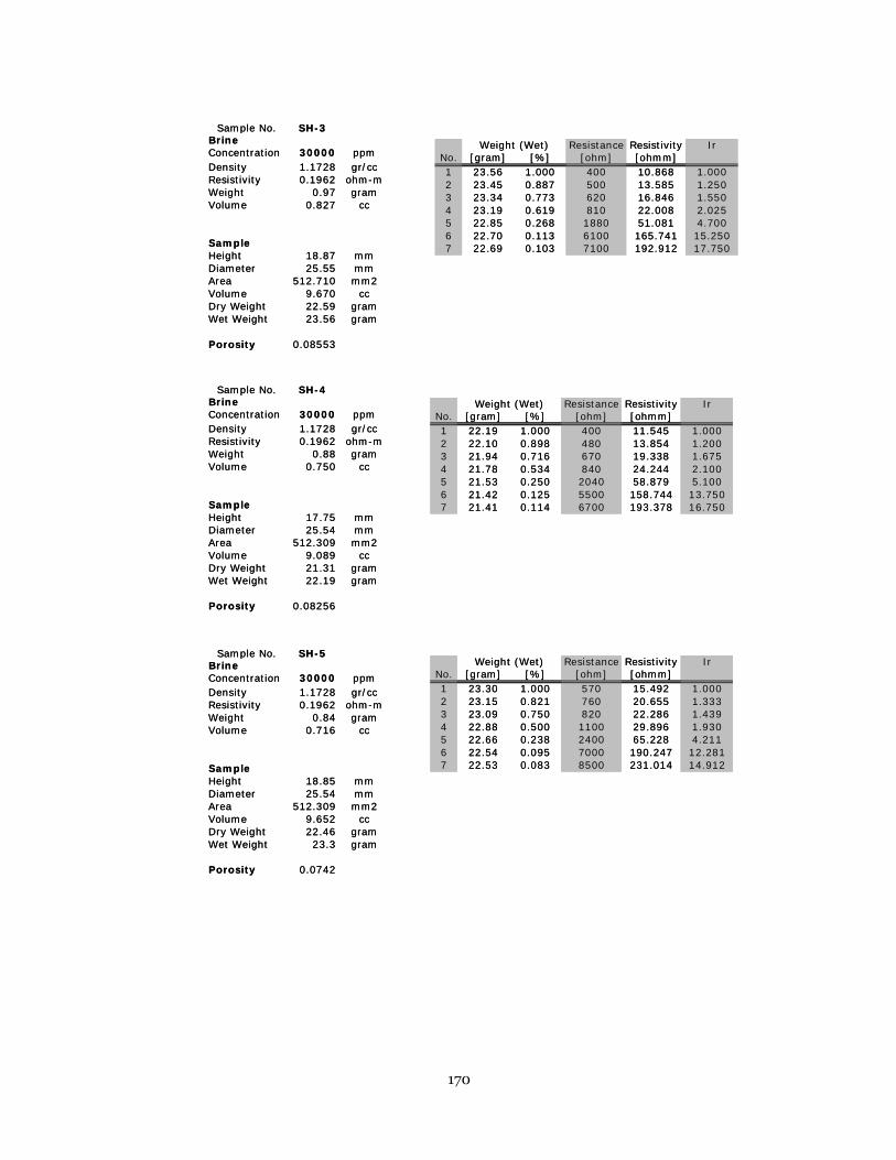
170

Resistance Resistivity IrNo. [gram] [%] [ohm] [ohmm]1 23.56 1.000 400 10.868 1.0002 23.45 0.887 500 13.585 1.2503 23.34 0.773 620 16.846 1.5504 23.19 0.619 810 22.008 2.0255 22.85 0.268 1880 51.081 4.7006 22.70 0.113 6100 165.741 15.2507 22.69 0.103 7100 192.912 17.750

Weight (Wet)

Sample No. SH-3Brine Concentration 30000 ppmDensity 1.1728 gr/ccResistivity 0.1962 ohm-mWeight 0.97 gramVolume 0.827 cc

SampleHeight 18.87 mmDiameter 25.55 mmArea 512.710 mm2Volume 9.670 ccDry Weight 22.59 gramWet Weight 23.56 gram

Porosity 0.08553

Resistance Resistivity IrNo. [gram] [%] [ohm] [ohmm]1 23.56 1.000 400 10.868 1.0002 23.45 0.887 500 13.585 1.2503 23.34 0.773 620 16.846 1.5504 23.19 0.619 810 22.008 2.0255 22.85 0.268 1880 51.081 4.7006 22.70 0.113 6100 165.741 15.2507 22.69 0.103 7100 192.912 17.750

Weight (Wet)

Sample No. SH-3Brine Concentration 30000 ppmDensity 1.1728 gr/ccResistivity 0.1962 ohm-mWeight 0.97 gramVolume 0.827 cc

SampleHeight 18.87 mmDiameter 25.55 mmArea 512.710 mm2Volume 9.670 ccDry Weight 22.59 gramWet Weight 23.56 gram

Porosity 0.08553

Resistance Resistivity IrNo. [gram] [%] [ohm] [ohmm]1 22.19 1.000 400 11.545 1.0002 22.10 0.898 480 13.854 1.2003 21.94 0.716 670 19.338 1.6754 21.78 0.534 840 24.244 2.1005 21.53 0.250 2040 58.879 5.1006 21.42 0.125 5500 158.744 13.7507 21.41 0.114 6700 193.378 16.750

Weight (Wet)Sample No. SH-4

Brine Concentration 30000 ppmDensity 1.1728 gr/ccResistivity 0.1962 ohm-mWeight 0.88 gramVolume 0.750 cc

SampleHeight 17.75 mmDiameter 25.54 mmArea 512.309 mm2Volume 9.089 ccDry Weight 21.31 gramWet Weight 22.19 gram

Porosity 0.08256

Resistance Resistivity IrNo. [gram] [%] [ohm] [ohmm]1 22.19 1.000 400 11.545 1.0002 22.10 0.898 480 13.854 1.2003 21.94 0.716 670 19.338 1.6754 21.78 0.534 840 24.244 2.1005 21.53 0.250 2040 58.879 5.1006 21.42 0.125 5500 158.744 13.7507 21.41 0.114 6700 193.378 16.750

Weight (Wet)Sample No. SH-4

Brine Concentration 30000 ppmDensity 1.1728 gr/ccResistivity 0.1962 ohm-mWeight 0.88 gramVolume 0.750 cc

SampleHeight 17.75 mmDiameter 25.54 mmArea 512.309 mm2Volume 9.089 ccDry Weight 21.31 gramWet Weight 22.19 gram

Porosity 0.08256

Resistance Resistivity IrNo. [gram] [%] [ohm] [ohmm]1 23.30 1.000 570 15.492 1.0002 23.15 0.821 760 20.655 1.3333 23.09 0.750 820 22.286 1.4394 22.88 0.500 1100 29.896 1.9305 22.66 0.238 2400 65.228 4.2116 22.54 0.095 7000 190.247 12.2817 22.53 0.083 8500 231.014 14.912

Weight (Wet)Sample No. SH-5

Brine Concentration 30000 ppmDensity 1.1728 gr/ccResistivity 0.1962 ohm-mWeight 0.84 gramVolume 0.716 cc

SampleHeight 18.85 mmDiameter 25.54 mmArea 512.309 mm2Volume 9.652 ccDry Weight 22.46 gramWet Weight 23.3 gram

Porosity 0.0742

Resistance Resistivity IrNo. [gram] [%] [ohm] [ohmm]1 23.30 1.000 570 15.492 1.0002 23.15 0.821 760 20.655 1.3333 23.09 0.750 820 22.286 1.4394 22.88 0.500 1100 29.896 1.9305 22.66 0.238 2400 65.228 4.2116 22.54 0.095 7000 190.247 12.2817 22.53 0.083 8500 231.014 14.912

Weight (Wet)Sample No. SH-5

Brine Concentration 30000 ppmDensity 1.1728 gr/ccResistivity 0.1962 ohm-mWeight 0.84 gramVolume 0.716 cc

SampleHeight 18.85 mmDiameter 25.54 mmArea 512.309 mm2Volume 9.652 ccDry Weight 22.46 gramWet Weight 23.3 gram

Porosity 0.0742

171

Resistance Resistivity IrNo. [gram] [%] [ohm] [ohmm]1 20.47 1.000 450 13.835 1.0002 20.38 0.883 620 19.062 1.3783 20.30 0.779 720 22.137 1.6004 20.07 0.481 1030 31.668 2.2895 19.86 0.208 2560 78.708 5.6896 19.77 0.091 6700 205.993 14.8897 19.77 0.091 6800 209.067 15.111

Weight (Wet)

Sample No. SH-6Brine Concentration 30000 ppmDensity 1.1728 gr/ccResistivity 0.1962 ohm-mWeight 0.77 gramVolume 0.657 cc

SampleHeight 16.65 mmDiameter 25.53 mmArea 511.908 mm2Volume 8.519 ccDry Weight 19.7 gramWet Weight 20.47 gram

Porosity 0.07707

Resistance Resistivity IrNo. [gram] [%] [ohm] [ohmm]1 20.47 1.000 450 13.835 1.0002 20.38 0.883 620 19.062 1.3783 20.30 0.779 720 22.137 1.6004 20.07 0.481 1030 31.668 2.2895 19.86 0.208 2560 78.708 5.6896 19.77 0.091 6700 205.993 14.8897 19.77 0.091 6800 209.067 15.111

Weight (Wet)

Sample No. SH-6Brine Concentration 30000 ppmDensity 1.1728 gr/ccResistivity 0.1962 ohm-mWeight 0.77 gramVolume 0.657 cc

SampleHeight 16.65 mmDiameter 25.53 mmArea 511.908 mm2Volume 8.519 ccDry Weight 19.7 gramWet Weight 20.47 gram

Porosity 0.07707

Resistance Resistivity IrNo. [gram] [%] [ohm] [ohmm]1 22.65 1.000 327 9.427 1.0002 22.50 0.805 560 16.145 1.7133 22.43 0.714 690 19.893 2.1104 22.23 0.455 1470 42.380 4.4955 22.03 0.195 4400 126.852 13.4566 21.99 0.143 12600 363.258 38.5327 21.98 0.130 7700 221.991 23.547

Weight (Wet)Sample No. SH-7

Brine Concentration 30000 ppmDensity 1.1728 gr/ccResistivity 0.1962 ohm-mWeight 0.77 gramVolume 0.657 cc

SampleHeight 17.77 mmDiameter 25.54 mmArea 512.309 mm2Volume 9.099 ccDry Weight 21.88 gramWet Weight 22.65 gram

Porosity 0.07216

Resistance Resistivity IrNo. [gram] [%] [ohm] [ohmm]1 22.65 1.000 327 9.427 1.0002 22.50 0.805 560 16.145 1.7133 22.43 0.714 690 19.893 2.1104 22.23 0.455 1470 42.380 4.4955 22.03 0.195 4400 126.852 13.4566 21.99 0.143 12600 363.258 38.5327 21.98 0.130 7700 221.991 23.547

Weight (Wet)Sample No. SH-7

Brine Concentration 30000 ppmDensity 1.1728 gr/ccResistivity 0.1962 ohm-mWeight 0.77 gramVolume 0.657 cc

SampleHeight 17.77 mmDiameter 25.54 mmArea 512.309 mm2Volume 9.099 ccDry Weight 21.88 gramWet Weight 22.65 gram

Porosity 0.07216

Resistance Resistivity IrNo. [gram] [%] [ohm] [ohmm]1 23.46 1.000 400 11.168 1.0002 23.38 0.900 500 13.960 1.2503 23.26 0.750 800 22.337 2.0004 23.15 0.612 970 27.083 2.4255 22.86 0.250 2740 76.503 6.8506 22.78 0.150 5300 147.980 13.2507 22.77 0.137 6100 170.316 15.250

Weight (Wet)Sample No. SH-8Brine Concentration 30000 ppmDensity 1.1728 gr/ccResistivity 0.1962 ohm-mWeight 0.8 gramVolume 0.682 cc

SampleHeight 18.32 mmDiameter 25.52 mmArea 511.507 mm2Volume 9.366 ccDry Weight 22.66 gramWet Weight 23.46 gram

Porosity 0.07283

Resistance Resistivity IrNo. [gram] [%] [ohm] [ohmm]1 23.46 1.000 400 11.168 1.0002 23.38 0.900 500 13.960 1.2503 23.26 0.750 800 22.337 2.0004 23.15 0.612 970 27.083 2.4255 22.86 0.250 2740 76.503 6.8506 22.78 0.150 5300 147.980 13.2507 22.77 0.137 6100 170.316 15.250

Weight (Wet)Sample No. SH-8Brine Concentration 30000 ppmDensity 1.1728 gr/ccResistivity 0.1962 ohm-mWeight 0.8 gramVolume 0.682 cc

SampleHeight 18.32 mmDiameter 25.52 mmArea 511.507 mm2Volume 9.366 ccDry Weight 22.66 gramWet Weight 23.46 gram

Porosity 0.07283

172

Resistance Resistivity IrNo. [gram] [%] [ohm] [ohmm]1 22.72 1.000 284 7.953 1.0002 22.61 0.866 420 11.762 1.4793 22.51 0.744 630 17.642 2.2184 22.43 0.646 960 26.884 3.3805 22.22 0.390 1520 42.566 5.3526 22.08 0.220 3600 100.813 12.6767 22.05 0.183 4400 123.216 15.493

Weight (Wet)Sample No. SH-10

Brine Concentration 30000 ppmDensity 1.1728 gr/ccResistivity 0.1962 ohm-mWeight 0.82 gramVolume 0.699 cc

SampleHeight 18.28 mmDiameter 25.53 mmArea 511.908 mm2Volume 9.353 ccDry Weight 21.9 gramWet Weight 22.72 gram

Porosity 0.07476

Resistance Resistivity IrNo. [gram] [%] [ohm] [ohmm]1 22.72 1.000 284 7.953 1.0002 22.61 0.866 420 11.762 1.4793 22.51 0.744 630 17.642 2.2184 22.43 0.646 960 26.884 3.3805 22.22 0.390 1520 42.566 5.3526 22.08 0.220 3600 100.813 12.6767 22.05 0.183 4400 123.216 15.493

Weight (Wet)Sample No. SH-10

Brine Concentration 30000 ppmDensity 1.1728 gr/ccResistivity 0.1962 ohm-mWeight 0.82 gramVolume 0.699 cc

SampleHeight 18.28 mmDiameter 25.53 mmArea 511.908 mm2Volume 9.353 ccDry Weight 21.9 gramWet Weight 22.72 gram

Porosity 0.07476

Resistance Resistivity IrNo. [gram] [%] [ohm] [ohmm]1 23.09 1.000 390 10.915 1.0002 23.00 0.886 510 14.274 1.3083 22.88 0.734 690 19.312 1.7694 22.67 0.468 1210 33.866 3.1035 22.52 0.278 2320 64.933 5.9496 22.45 0.190 4400 123.149 11.2827 22.42 0.152 5600 156.735 14.359

Weight (Wet)

Sample No. SH-11Brine Concentration 30000 ppmDensity 1.1728 gr/ccResistivity 0.1962 ohm-mWeight 0.79 gramVolume 0.674 cc

SampleHeight 18.29 mmDiameter 25.53 mmArea 511.908 mm2Volume 9.358 ccDry Weight 22.3 gramWet Weight 23.09 gram

Porosity 0.07198

Resistance Resistivity IrNo. [gram] [%] [ohm] [ohmm]1 23.09 1.000 390 10.915 1.0002 23.00 0.886 510 14.274 1.3083 22.88 0.734 690 19.312 1.7694 22.67 0.468 1210 33.866 3.1035 22.52 0.278 2320 64.933 5.9496 22.45 0.190 4400 123.149 11.2827 22.42 0.152 5600 156.735 14.359

Weight (Wet)

Sample No. SH-11Brine Concentration 30000 ppmDensity 1.1728 gr/ccResistivity 0.1962 ohm-mWeight 0.79 gramVolume 0.674 cc

SampleHeight 18.29 mmDiameter 25.53 mmArea 511.908 mm2Volume 9.358 ccDry Weight 22.3 gramWet Weight 23.09 gram

Porosity 0.07198

Sample No. SH-13Brine Concentration 30000 ppmDensity 1.1728 gr/ccResistivity 0.1962 ohm-mWeight 0.94 gramVolume 0.802 cc

SampleHeight 19.86 mmDiameter 25.54 mmArea 512.309 mm2Volume 10.169 ccDry Weight 23.02 gramWet Weight 23.96 gram

Porosity 0.07882

Resistance Resistivity IrNo. [gram] [%] [ohm] [ohmm]1 23.96 1.000 240 6.191 1.0002 23.74 0.766 570 14.704 2.3753 23.61 0.628 930 23.990 3.8754 23.45 0.457 1680 43.337 7.0005 23.22 0.213 4900 126.400 20.4176 23.16 0.149 8500 219.266 35.4177 23.14 0.128 9500 245.062 39.583

Weight (Wet)Sample No. SH-13

Brine Concentration 30000 ppmDensity 1.1728 gr/ccResistivity 0.1962 ohm-mWeight 0.94 gramVolume 0.802 cc

SampleHeight 19.86 mmDiameter 25.54 mmArea 512.309 mm2Volume 10.169 ccDry Weight 23.02 gramWet Weight 23.96 gram

Porosity 0.07882

Resistance Resistivity IrNo. [gram] [%] [ohm] [ohmm]1 23.96 1.000 240 6.191 1.0002 23.74 0.766 570 14.704 2.3753 23.61 0.628 930 23.990 3.8754 23.45 0.457 1680 43.337 7.0005 23.22 0.213 4900 126.400 20.4176 23.16 0.149 8500 219.266 35.4177 23.14 0.128 9500 245.062 39.583

Weight (Wet)

173

APPENDIX D DATA OF SHALY SAND ELECTRICAL MEASUREMENT

174

A. 3,000 ppm NaCl Salinity

Sample No. SHY-1Brine Concentration 3000 ppmDensity 1.1504 gr/ccResistivity 1.342 ohm-mWeight 1.66 gramVolume 1.443 cc

SampleHeight 38.85 mmDiameter 25.53 mmArea 511.908 mm2Volume 19.878 ccDry Weight 47.19 gramWet Weight 48.85 gram

Porosity 0.07259

Resistance Resistivity IrNo. [gram] [%] [ohm] [ohmm]1 48.85 1.000 1530 20.160 1.0002 48.77 0.952 1600 21.082 1.0463 48.73 0.928 1610 21.214 1.0524 48.69 0.904 1640 21.609 1.0725 48.64 0.873 1670 22.005 1.0926 48.56 0.825 1780 23.454 1.1637 48.49 0.783 1920 25.299 1.2558 48.26 0.645 2570 33.864 1.6809 47.73 0.325 6000 79.059 3.92210 47.62 0.259 8500 112.000 5.55611 47.58 0.235 10000 131.765 6.53612 47.45 0.157 20500 270.119 13.399

Weight (Wet)

Sample No. SHY-1Brine Concentration 3000 ppmDensity 1.1504 gr/ccResistivity 1.342 ohm-mWeight 1.66 gramVolume 1.443 cc

SampleHeight 38.85 mmDiameter 25.53 mmArea 511.908 mm2Volume 19.878 ccDry Weight 47.19 gramWet Weight 48.85 gram

Porosity 0.07259

Resistance Resistivity IrNo. [gram] [%] [ohm] [ohmm]1 48.85 1.000 1530 20.160 1.0002 48.77 0.952 1600 21.082 1.0463 48.73 0.928 1610 21.214 1.0524 48.69 0.904 1640 21.609 1.0725 48.64 0.873 1670 22.005 1.0926 48.56 0.825 1780 23.454 1.1637 48.49 0.783 1920 25.299 1.2558 48.26 0.645 2570 33.864 1.6809 47.73 0.325 6000 79.059 3.92210 47.62 0.259 8500 112.000 5.55611 47.58 0.235 10000 131.765 6.53612 47.45 0.157 20500 270.119 13.399

Weight (Wet)

Sample No. SHY-2Brine Concentration 3000 ppmDensity 1.1504 gr/ccResistivity 1.342 ohm-mWeight 2.2 gramVolume 1.912 cc

SampleHeight 37.76 mmDiameter 25.53 mmArea 511.908 mm2Volume 19.320 ccDry Weight 44.06 gramWet Weight 46.26 gram

Porosity 0.09899

Resistance Resistivity IrNo. [gram] [%] [ohm] [ohmm]1 46.26 1.000 2660 36.061 1.0002 46.18 0.964 2610 35.383 0.9813 46.11 0.932 2540 34.434 0.9554 46.06 0.909 1760 23.860 0.6625 45.94 0.855 1770 23.996 0.6656 45.53 0.668 2090 28.334 0.7867 45.38 0.600 2430 32.943 0.9148 44.59 0.241 6800 92.187 2.5569 44.46 0.182 9000 122.012 3.38310 44.36 0.136 13500 183.018 5.07511 44.23 0.077 40000 542.275 15.038

Weight (Wet)

Sample No. SHY-2Brine Concentration 3000 ppmDensity 1.1504 gr/ccResistivity 1.342 ohm-mWeight 2.2 gramVolume 1.912 cc

SampleHeight 37.76 mmDiameter 25.53 mmArea 511.908 mm2Volume 19.320 ccDry Weight 44.06 gramWet Weight 46.26 gram

Porosity 0.09899

Resistance Resistivity IrNo. [gram] [%] [ohm] [ohmm]1 46.26 1.000 2660 36.061 1.0002 46.18 0.964 2610 35.383 0.9813 46.11 0.932 2540 34.434 0.9554 46.06 0.909 1760 23.860 0.6625 45.94 0.855 1770 23.996 0.6656 45.53 0.668 2090 28.334 0.7867 45.38 0.600 2430 32.943 0.9148 44.59 0.241 6800 92.187 2.5569 44.46 0.182 9000 122.012 3.38310 44.36 0.136 13500 183.018 5.07511 44.23 0.077 40000 542.275 15.038

Weight (Wet)

Sample No. SHY-3Brine Concentration 3000 ppmDensity 1.1504 gr/ccResistivity 1.342 ohm-mWeight 2.07 gramVolume 1.799 cc

SampleHeight 39.97 mmDiameter 25.52 mmArea 511.507 mm2Volume 20.435 ccDry Weight 46.43 gramWet Weight 48.5 gram

Porosity 0.08806

Resistance Resistivity IrNo. [gram] [%] [ohm] [ohmm]1 48.50 1.000 1630 20.860 1.0002 48.46 0.981 1630 20.860 1.0003 48.41 0.957 1740 22.267 1.0674 48.34 0.923 1790 22.907 1.0985 48.29 0.899 1710 21.883 1.0496 48.15 0.831 1820 23.291 1.1177 48.05 0.783 1960 25.083 1.2028 47.82 0.671 2480 31.737 1.5219 47.18 0.362 3900 49.909 2.39310 47.01 0.280 4800 61.427 2.94511 46.85 0.203 7300 93.420 4.47912 46.65 0.106 19100 244.428 11.718

Weight (Wet)

Sample No. SHY-3Brine Concentration 3000 ppmDensity 1.1504 gr/ccResistivity 1.342 ohm-mWeight 2.07 gramVolume 1.799 cc

SampleHeight 39.97 mmDiameter 25.52 mmArea 511.507 mm2Volume 20.435 ccDry Weight 46.43 gramWet Weight 48.5 gram

Porosity 0.08806

Resistance Resistivity IrNo. [gram] [%] [ohm] [ohmm]1 48.50 1.000 1630 20.860 1.0002 48.46 0.981 1630 20.860 1.0003 48.41 0.957 1740 22.267 1.0674 48.34 0.923 1790 22.907 1.0985 48.29 0.899 1710 21.883 1.0496 48.15 0.831 1820 23.291 1.1177 48.05 0.783 1960 25.083 1.2028 47.82 0.671 2480 31.737 1.5219 47.18 0.362 3900 49.909 2.39310 47.01 0.280 4800 61.427 2.94511 46.85 0.203 7300 93.420 4.47912 46.65 0.106 19100 244.428 11.718

Weight (Wet)

175

Sample No. SHY-4Brine Concentration 3000 ppmDensity 1.1504 gr/ccResistivity 1.342 ohm-mWeight 1.96 gramVolume 1.704 cc

SampleHeight 36.66 mmDiameter 25.53 mmArea 511.908 mm2Volume 18.757 ccDry Weight 45.49 gramWet Weight 47.45 gram

Porosity 0.09083

Resistance Resistivity IrNo. [gram] [%] [ohm] [ohmm]1 47.45 1.000 1290 18.013 1.0002 47.33 0.939 1310 18.292 1.0163 47.23 0.888 1420 19.828 1.1014 46.88 0.709 1530 21.364 1.1865 46.82 0.679 1570 21.923 1.2176 46.69 0.612 2340 32.675 1.8147 46.60 0.566 2460 34.351 1.9078 46.13 0.327 5400 75.404 4.1869 46.08 0.301 5700 79.593 4.41910 46.01 0.265 7200 100.538 5.58111 45.77 0.143 20500 286.255 15.891

Weight (Wet)

Sample No. SHY-4Brine Concentration 3000 ppmDensity 1.1504 gr/ccResistivity 1.342 ohm-mWeight 1.96 gramVolume 1.704 cc

SampleHeight 36.66 mmDiameter 25.53 mmArea 511.908 mm2Volume 18.757 ccDry Weight 45.49 gramWet Weight 47.45 gram

Porosity 0.09083

Resistance Resistivity IrNo. [gram] [%] [ohm] [ohmm]1 47.45 1.000 1290 18.013 1.0002 47.33 0.939 1310 18.292 1.0163 47.23 0.888 1420 19.828 1.1014 46.88 0.709 1530 21.364 1.1865 46.82 0.679 1570 21.923 1.2176 46.69 0.612 2340 32.675 1.8147 46.60 0.566 2460 34.351 1.9078 46.13 0.327 5400 75.404 4.1869 46.08 0.301 5700 79.593 4.41910 46.01 0.265 7200 100.538 5.58111 45.77 0.143 20500 286.255 15.891

Weight (Wet)

Sample No. SHY-5Brine Concentration 3000 ppmDensity 1.1504 gr/ccResistivity 1.342 ohm-mWeight 1.98 gramVolume 1.721 cc

SampleHeight 39.99 mmDiameter 25.53 mmArea 511.908 mm2Volume 20.461 ccDry Weight 48.41 gramWet Weight 50.39 gram

Porosity 0.08412

Resistance Resistivity IrNo. [gram] [%] [ohm] [ohmm]1 50.39 1.000 2000 25.602 1.0002 50.37 0.990 2020 25.858 1.0103 50.27 0.939 2420 30.978 1.2104 50.13 0.869 2300 29.442 1.1505 50.08 0.843 2310 29.570 1.1556 49.95 0.778 2560 32.770 1.2807 49.89 0.747 2720 34.818 1.3608 49.72 0.662 3220 41.219 1.6109 49.20 0.399 5700 72.965 2.85010 49.05 0.323 7500 96.007 3.75011 48.99 0.293 8800 112.648 4.40012 48.80 0.197 21100 270.099 10.550

Weight (Wet)

Sample No. SHY-5Brine Concentration 3000 ppmDensity 1.1504 gr/ccResistivity 1.342 ohm-mWeight 1.98 gramVolume 1.721 cc

SampleHeight 39.99 mmDiameter 25.53 mmArea 511.908 mm2Volume 20.461 ccDry Weight 48.41 gramWet Weight 50.39 gram

Porosity 0.08412

Resistance Resistivity IrNo. [gram] [%] [ohm] [ohmm]1 50.39 1.000 2000 25.602 1.0002 50.37 0.990 2020 25.858 1.0103 50.27 0.939 2420 30.978 1.2104 50.13 0.869 2300 29.442 1.1505 50.08 0.843 2310 29.570 1.1556 49.95 0.778 2560 32.770 1.2807 49.89 0.747 2720 34.818 1.3608 49.72 0.662 3220 41.219 1.6109 49.20 0.399 5700 72.965 2.85010 49.05 0.323 7500 96.007 3.75011 48.99 0.293 8800 112.648 4.40012 48.80 0.197 21100 270.099 10.550

Weight (Wet)

Sample No. SHY-6Brine Concentration 3000 ppmDensity 1.1504 gr/ccResistivity 1.342 ohm-mWeight 2.18 gramVolume 1.895 cc

SampleHeight 34.98 mmDiameter 25.53 mmArea 511.908 mm2Volume 17.897 ccDry Weight 41.1 gramWet Weight 43.28 gram

Porosity 0.10588

Resistance Resistivity IrNo. [gram] [%] [ohm] [ohmm]1 43.28 1.000 1280 18.732 1.0002 43.22 0.972 1540 22.537 1.2033 43.06 0.899 1610 23.561 1.2584 42.56 0.670 2140 31.317 1.6725 42.48 0.633 2200 32.195 1.7196 42.29 0.546 2640 38.635 2.0637 42.18 0.495 3010 44.049 2.3528 41.56 0.211 7200 105.367 5.6259 41.40 0.138 11900 174.148 9.29710 41.31 0.096 20700 302.930 16.17211 41.22 0.055 50000 731.715 39.063

Weight (Wet)

Sample No. SHY-6Brine Concentration 3000 ppmDensity 1.1504 gr/ccResistivity 1.342 ohm-mWeight 2.18 gramVolume 1.895 cc

SampleHeight 34.98 mmDiameter 25.53 mmArea 511.908 mm2Volume 17.897 ccDry Weight 41.1 gramWet Weight 43.28 gram

Porosity 0.10588

Resistance Resistivity IrNo. [gram] [%] [ohm] [ohmm]1 43.28 1.000 1280 18.732 1.0002 43.22 0.972 1540 22.537 1.2033 43.06 0.899 1610 23.561 1.2584 42.56 0.670 2140 31.317 1.6725 42.48 0.633 2200 32.195 1.7196 42.29 0.546 2640 38.635 2.0637 42.18 0.495 3010 44.049 2.3528 41.56 0.211 7200 105.367 5.6259 41.40 0.138 11900 174.148 9.29710 41.31 0.096 20700 302.930 16.17211 41.22 0.055 50000 731.715 39.063

Weight (Wet)

176

Sample No. SHY-7Brine Concentration 3000 ppmDensity 1.1504 gr/ccResistivity 1.342 ohm-mWeight 1.68 gramVolume 1.460 cc

SampleHeight 37.67 mmDiameter 25.52 mmArea 511.507 mm2Volume 19.259 ccDry Weight 44.98 gramWet Weight 46.66 gram

Porosity 0.07583

Resistance Resistivity IrNo. [gram] [%] [ohm] [ohmm]1 46.66 1.000 2030 27.565 1.0002 46.61 0.970 2100 28.515 1.0343 46.55 0.935 2200 29.873 1.0844 46.44 0.869 2360 32.046 1.1635 46.41 0.851 2410 32.724 1.1876 46.27 0.768 2960 40.193 1.4587 46.18 0.714 2910 39.514 1.4338 46.13 0.685 3000 40.736 1.4789 45.65 0.399 5300 71.967 2.61110 45.52 0.321 6600 89.619 3.25111 45.41 0.256 9400 127.639 4.63112 45.25 0.161 24200 328.603 11.921

Weight (Wet)

Sample No. SHY-7Brine Concentration 3000 ppmDensity 1.1504 gr/ccResistivity 1.342 ohm-mWeight 1.68 gramVolume 1.460 cc

SampleHeight 37.67 mmDiameter 25.52 mmArea 511.507 mm2Volume 19.259 ccDry Weight 44.98 gramWet Weight 46.66 gram

Porosity 0.07583

Resistance Resistivity IrNo. [gram] [%] [ohm] [ohmm]1 46.66 1.000 2030 27.565 1.0002 46.61 0.970 2100 28.515 1.0343 46.55 0.935 2200 29.873 1.0844 46.44 0.869 2360 32.046 1.1635 46.41 0.851 2410 32.724 1.1876 46.27 0.768 2960 40.193 1.4587 46.18 0.714 2910 39.514 1.4338 46.13 0.685 3000 40.736 1.4789 45.65 0.399 5300 71.967 2.61110 45.52 0.321 6600 89.619 3.25111 45.41 0.256 9400 127.639 4.63112 45.25 0.161 24200 328.603 11.921

Weight (Wet)

Sample No. SHY-9Brine Concentration 3000 ppmDensity 1.1504 gr/ccResistivity 1.342 ohm-mWeight 1.55 gramVolume 1.347 cc

SampleHeight 33.28 mmDiameter 25.51 mmArea 511.106 mm2Volume 17.001 ccDry Weight 40.08 gramWet Weight 41.63 gram

Porosity 0.07925

Resistance Resistivity IrNo. [gram] [%] [ohm] [ohmm]1 41.63 1.000 1600 24.572 1.0002 41.60 0.981 1660 25.494 1.0383 41.54 0.942 1740 26.722 1.0884 41.45 0.884 1900 29.180 1.1885 41.40 0.852 1910 29.333 1.1946 41.29 0.781 2120 32.558 1.3257 41.22 0.735 2300 35.323 1.4388 41.03 0.613 2920 44.845 1.8259 40.82 0.477 3900 59.895 2.43810 40.67 0.381 4800 73.717 3.00011 40.57 0.316 6100 93.682 3.81312 40.37 0.187 18100 277.975 11.313

Weight (Wet)

Sample No. SHY-9Brine Concentration 3000 ppmDensity 1.1504 gr/ccResistivity 1.342 ohm-mWeight 1.55 gramVolume 1.347 cc

SampleHeight 33.28 mmDiameter 25.51 mmArea 511.106 mm2Volume 17.001 ccDry Weight 40.08 gramWet Weight 41.63 gram

Porosity 0.07925

Resistance Resistivity IrNo. [gram] [%] [ohm] [ohmm]1 41.63 1.000 1600 24.572 1.0002 41.60 0.981 1660 25.494 1.0383 41.54 0.942 1740 26.722 1.0884 41.45 0.884 1900 29.180 1.1885 41.40 0.852 1910 29.333 1.1946 41.29 0.781 2120 32.558 1.3257 41.22 0.735 2300 35.323 1.4388 41.03 0.613 2920 44.845 1.8259 40.82 0.477 3900 59.895 2.43810 40.67 0.381 4800 73.717 3.00011 40.57 0.316 6100 93.682 3.81312 40.37 0.187 18100 277.975 11.313

Weight (Wet)

Sample No. SHY-10Brine Concentration 3000 ppmDensity 1.1504 gr/ccResistivity 1.342 ohm-mWeight 1.71 gramVolume 1.486 cc

SampleHeight 38.84 mmDiameter 25.51 mmArea 511.106 mm2Volume 19.841 ccDry Weight 46.61 gramWet Weight 48.32 gram

Porosity 0.07492

Resistance Resistivity IrNo. [gram] [%] [ohm] [ohmm]1 48.32 1.000 1880 24.739 1.0002 48.29 0.982 1900 25.003 1.0113 48.16 0.906 2090 27.503 1.1124 48.01 0.819 2270 29.872 1.2075 47.91 0.760 2390 31.451 1.2716 47.75 0.667 2850 37.504 1.5167 47.66 0.614 3130 41.188 1.6658 47.66 0.614 3190 41.978 1.6979 47.46 0.497 4000 52.637 2.12810 47.27 0.386 5100 67.112 2.71311 47.14 0.310 7000 92.115 3.72312 46.94 0.193 19500 256.606 10.372

Weight (Wet)

Sample No. SHY-10Brine Concentration 3000 ppmDensity 1.1504 gr/ccResistivity 1.342 ohm-mWeight 1.71 gramVolume 1.486 cc

SampleHeight 38.84 mmDiameter 25.51 mmArea 511.106 mm2Volume 19.841 ccDry Weight 46.61 gramWet Weight 48.32 gram

Porosity 0.07492

Resistance Resistivity IrNo. [gram] [%] [ohm] [ohmm]1 48.32 1.000 1880 24.739 1.0002 48.29 0.982 1900 25.003 1.0113 48.16 0.906 2090 27.503 1.1124 48.01 0.819 2270 29.872 1.2075 47.91 0.760 2390 31.451 1.2716 47.75 0.667 2850 37.504 1.5167 47.66 0.614 3130 41.188 1.6658 47.66 0.614 3190 41.978 1.6979 47.46 0.497 4000 52.637 2.12810 47.27 0.386 5100 67.112 2.71311 47.14 0.310 7000 92.115 3.72312 46.94 0.193 19500 256.606 10.372

Weight (Wet)

177

Sample No. SHY-11Brine Concentration 3000 ppmDensity 1.1504 gr/ccResistivity 1.342 ohm-mWeight 2.12 gramVolume 1.843 cc

SampleHeight 40.54 mmDiameter 25.53 mmArea 511.908 mm2Volume 20.742 ccDry Weight 47.86 gramWet Weight 49.98 gram

Porosity 0.08884

Resistance Resistivity IrNo. [gram] [%] [ohm] [ohmm]1 49.98 1.000 2250 28.411 1.0002 49.92 0.972 2370 29.927 1.0533 49.85 0.939 2520 31.821 1.1204 49.76 0.896 2610 32.957 1.1605 49.69 0.863 2690 33.967 1.1966 49.54 0.792 2970 37.503 1.3207 49.45 0.750 2930 36.998 1.3028 48.46 0.283 6900 87.128 3.0679 48.33 0.222 9100 114.908 4.04410 48.23 0.175 13400 169.205 5.95611 48.06 0.094 50000 631.361 22.222

Weight (Wet)

Sample No. SHY-11Brine Concentration 3000 ppmDensity 1.1504 gr/ccResistivity 1.342 ohm-mWeight 2.12 gramVolume 1.843 cc

SampleHeight 40.54 mmDiameter 25.53 mmArea 511.908 mm2Volume 20.742 ccDry Weight 47.86 gramWet Weight 49.98 gram

Porosity 0.08884

Resistance Resistivity IrNo. [gram] [%] [ohm] [ohmm]1 49.98 1.000 2250 28.411 1.0002 49.92 0.972 2370 29.927 1.0533 49.85 0.939 2520 31.821 1.1204 49.76 0.896 2610 32.957 1.1605 49.69 0.863 2690 33.967 1.1966 49.54 0.792 2970 37.503 1.3207 49.45 0.750 2930 36.998 1.3028 48.46 0.283 6900 87.128 3.0679 48.33 0.222 9100 114.908 4.04410 48.23 0.175 13400 169.205 5.95611 48.06 0.094 50000 631.361 22.222

Weight (Wet)

Sample No. SHY-12Brine Concentration 3000 ppmDensity 1.1504 gr/ccResistivity 1.342 ohm-mWeight 1.71 gramVolume 1.486 cc

SampleHeight 38.34 mmDiameter 25.51 mmArea 511.106 mm2Volume 19.586 ccDry Weight 46 gramWet Weight 47.71 gram

Porosity 0.07589

Resistance Resistivity IrNo. [gram] [%] [ohm] [ohmm]1 47.71 1.000 2110 28.128 1.0002 47.66 0.971 2180 29.061 1.0333 47.60 0.936 2260 30.128 1.0714 47.52 0.889 2290 30.528 1.0855 47.44 0.842 2380 31.727 1.1286 47.36 0.795 2520 33.594 1.1947 47.27 0.743 2750 36.660 1.3038 47.14 0.667 3160 42.126 1.4989 46.47 0.275 8800 117.312 4.17110 46.38 0.222 12900 171.968 6.11411 46.36 0.211 15000 199.963 7.10912 46.23 0.135 46000 613.220 21.801

Weight (Wet)Sample No. SHY-12

Brine Concentration 3000 ppmDensity 1.1504 gr/ccResistivity 1.342 ohm-mWeight 1.71 gramVolume 1.486 cc

SampleHeight 38.34 mmDiameter 25.51 mmArea 511.106 mm2Volume 19.586 ccDry Weight 46 gramWet Weight 47.71 gram

Porosity 0.07589

Resistance Resistivity IrNo. [gram] [%] [ohm] [ohmm]1 47.71 1.000 2110 28.128 1.0002 47.66 0.971 2180 29.061 1.0333 47.60 0.936 2260 30.128 1.0714 47.52 0.889 2290 30.528 1.0855 47.44 0.842 2380 31.727 1.1286 47.36 0.795 2520 33.594 1.1947 47.27 0.743 2750 36.660 1.3038 47.14 0.667 3160 42.126 1.4989 46.47 0.275 8800 117.312 4.17110 46.38 0.222 12900 171.968 6.11411 46.36 0.211 15000 199.963 7.10912 46.23 0.135 46000 613.220 21.801

Weight (Wet)

Sample No. SHY-13Brine Concentration 3000 ppmDensity 1.1504 gr/ccResistivity 1.342 ohm-mWeight 2.15 gramVolume 1.869 cc

SampleHeight 40.55 mmDiameter 25.51 mmArea 511.106 mm2Volume 20.715 ccDry Weight 46.71 gramWet Weight 48.86 gram

Porosity 0.09022

Resistance Resistivity IrNo. [gram] [%] [ohm] [ohmm]1 48.86 1.000 2150 27.099 1.0002 48.80 0.972 2390 30.124 1.1123 48.75 0.949 2410 30.376 1.1214 48.69 0.921 2430 30.629 1.1305 48.64 0.898 2460 31.007 1.1446 48.44 0.805 2710 34.158 1.2607 48.30 0.740 2900 36.553 1.3498 48.10 0.647 3220 40.586 1.4989 47.49 0.363 5100 64.282 2.37210 47.28 0.265 7100 89.491 3.30211 47.18 0.219 8900 112.179 4.14012 46.98 0.126 26900 339.057 12.512

Weight (Wet)Sample No. SHY-13

Brine Concentration 3000 ppmDensity 1.1504 gr/ccResistivity 1.342 ohm-mWeight 2.15 gramVolume 1.869 cc

SampleHeight 40.55 mmDiameter 25.51 mmArea 511.106 mm2Volume 20.715 ccDry Weight 46.71 gramWet Weight 48.86 gram

Porosity 0.09022

Resistance Resistivity IrNo. [gram] [%] [ohm] [ohmm]1 48.86 1.000 2150 27.099 1.0002 48.80 0.972 2390 30.124 1.1123 48.75 0.949 2410 30.376 1.1214 48.69 0.921 2430 30.629 1.1305 48.64 0.898 2460 31.007 1.1446 48.44 0.805 2710 34.158 1.2607 48.30 0.740 2900 36.553 1.3498 48.10 0.647 3220 40.586 1.4989 47.49 0.363 5100 64.282 2.37210 47.28 0.265 7100 89.491 3.30211 47.18 0.219 8900 112.179 4.14012 46.98 0.126 26900 339.057 12.512

Weight (Wet)

178

B. 10,000 ppm NaCl Salinity

Sample No. SHY-1Brine Concentration 10000 ppmDensity 1.1556 gr/ccResistivity 0.5244 ohm-mWeight 1.62 gramVolume 1.402 cc

SampleHeight 38.85 mmDiameter 25.53 mmArea 511.908 mm2Volume 19.878 ccDry Weight 47.25 gramWet Weight 48.87 gram

Porosity 0.07053

Resistance Resistivity IrNo. [gram] [%] [ohm] [ohmm]1 48.87 1.000 1420 18.711 1.0002 48.73 0.914 1480 19.501 1.0423 48.66 0.870 1570 20.687 1.1064 48.59 0.827 1660 21.873 1.1695 48.46 0.747 1790 23.586 1.2616 48.41 0.716 1810 23.849 1.2757 48.32 0.660 2000 26.353 1.4088 48.21 0.593 2490 32.810 1.7549 48.05 0.494 3060 40.320 2.15510 47.85 0.370 4600 60.612 3.23911 47.78 0.327 5300 69.836 3.73212 47.76 0.315 5600 73.788 3.94413 47.68 0.265 6800 89.600 4.789

Weight (Wet)

Sample No. SHY-1Brine Concentration 10000 ppmDensity 1.1556 gr/ccResistivity 0.5244 ohm-mWeight 1.62 gramVolume 1.402 cc

SampleHeight 38.85 mmDiameter 25.53 mmArea 511.908 mm2Volume 19.878 ccDry Weight 47.25 gramWet Weight 48.87 gram

Porosity 0.07053

Resistance Resistivity IrNo. [gram] [%] [ohm] [ohmm]1 48.87 1.000 1420 18.711 1.0002 48.73 0.914 1480 19.501 1.0423 48.66 0.870 1570 20.687 1.1064 48.59 0.827 1660 21.873 1.1695 48.46 0.747 1790 23.586 1.2616 48.41 0.716 1810 23.849 1.2757 48.32 0.660 2000 26.353 1.4088 48.21 0.593 2490 32.810 1.7549 48.05 0.494 3060 40.320 2.15510 47.85 0.370 4600 60.612 3.23911 47.78 0.327 5300 69.836 3.73212 47.76 0.315 5600 73.788 3.94413 47.68 0.265 6800 89.600 4.789

Weight (Wet)

Sample No. SHY-2Brine Concentration 10000 ppmDensity 1.1556 gr/ccResistivity 0.5244 ohm-mWeight 2.13 gramVolume 1.843 cc

SampleHeight 37.76 mmDiameter 25.53 mmArea 511.908 mm2Volume 19.320 ccDry Weight 44.14 gramWet Weight 46.27 gram

Porosity 0.0954

Resistance Resistivity IrNo. [gram] [%] [ohm] [ohmm]1 46.27 1.000 1320 17.895 1.0002 45.85 0.803 1610 21.827 1.2203 45.75 0.756 1650 22.369 1.2504 45.69 0.728 1670 22.640 1.2655 45.45 0.615 1830 24.809 1.3866 45.36 0.573 1950 26.436 1.4777 44.91 0.362 3230 43.789 2.4478 44.90 0.357 3400 46.093 2.5769 44.80 0.310 3800 51.516 2.87910 44.60 0.216 5600 75.918 4.24211 44.51 0.174 6900 93.542 5.22712 44.48 0.160 7400 100.321 5.60613 44.38 0.113 10500 142.347 7.955

Weight (Wet)

Sample No. SHY-2Brine Concentration 10000 ppmDensity 1.1556 gr/ccResistivity 0.5244 ohm-mWeight 2.13 gramVolume 1.843 cc

SampleHeight 37.76 mmDiameter 25.53 mmArea 511.908 mm2Volume 19.320 ccDry Weight 44.14 gramWet Weight 46.27 gram

Porosity 0.0954

Resistance Resistivity IrNo. [gram] [%] [ohm] [ohmm]1 46.27 1.000 1320 17.895 1.0002 45.85 0.803 1610 21.827 1.2203 45.75 0.756 1650 22.369 1.2504 45.69 0.728 1670 22.640 1.2655 45.45 0.615 1830 24.809 1.3866 45.36 0.573 1950 26.436 1.4777 44.91 0.362 3230 43.789 2.4478 44.90 0.357 3400 46.093 2.5769 44.80 0.310 3800 51.516 2.87910 44.60 0.216 5600 75.918 4.24211 44.51 0.174 6900 93.542 5.22712 44.48 0.160 7400 100.321 5.60613 44.38 0.113 10500 142.347 7.955

Weight (Wet)

Sample No. SHY-3Brine Concentration 10000 ppmDensity 1.1556 gr/ccResistivity 0.5244 ohm-mWeight 1.98 gramVolume 1.713 cc

SampleHeight 39.97 mmDiameter 25.52 mmArea 511.507 mm2Volume 20.435 ccDry Weight 46.52 gramWet Weight 48.5 gram

Porosity 0.08385

Resistance Resistivity IrNo. [gram] [%] [ohm] [ohmm]1 48.50 1.000 1270 16.253 1.0002 48.33 0.914 1530 19.580 1.2053 48.21 0.854 1790 22.907 1.4094 48.04 0.768 1850 23.675 1.4575 47.89 0.692 2730 34.937 2.1506 47.68 0.586 1970 25.211 1.5517 47.50 0.495 2150 27.514 1.6938 47.13 0.308 3400 43.511 2.6779 46.96 0.222 4500 57.588 3.54310 46.87 0.177 6100 78.063 4.80311 46.81 0.146 7300 93.420 5.74812 46.80 0.141 7700 98.539 6.06313 46.77 0.126 8500 108.777 6.693

Weight (Wet)

Sample No. SHY-3Brine Concentration 10000 ppmDensity 1.1556 gr/ccResistivity 0.5244 ohm-mWeight 1.98 gramVolume 1.713 cc

SampleHeight 39.97 mmDiameter 25.52 mmArea 511.507 mm2Volume 20.435 ccDry Weight 46.52 gramWet Weight 48.5 gram

Porosity 0.08385

Resistance Resistivity IrNo. [gram] [%] [ohm] [ohmm]1 48.50 1.000 1270 16.253 1.0002 48.33 0.914 1530 19.580 1.2053 48.21 0.854 1790 22.907 1.4094 48.04 0.768 1850 23.675 1.4575 47.89 0.692 2730 34.937 2.1506 47.68 0.586 1970 25.211 1.5517 47.50 0.495 2150 27.514 1.6938 47.13 0.308 3400 43.511 2.6779 46.96 0.222 4500 57.588 3.54310 46.87 0.177 6100 78.063 4.80311 46.81 0.146 7300 93.420 5.74812 46.80 0.141 7700 98.539 6.06313 46.77 0.126 8500 108.777 6.693

Weight (Wet)

179

Sample No. SHY-4Brine Concentration 10000 ppmDensity 1.1556 gr/ccResistivity 0.5244 ohm-mWeight 1.98 gramVolume 1.713 cc

SampleHeight 36.66 mmDiameter 25.53 mmArea 511.908 mm2Volume 18.757 ccDry Weight 45.43 gramWet Weight 47.41 gram

Porosity 0.09135

Resistance Resistivity IrNo. [gram] [%] [ohm] [ohmm]1 47.41 1.000 1030 14.383 1.0002 46.75 0.667 1870 26.112 1.8163 46.70 0.641 2010 28.067 1.9514 46.66 0.621 2390 33.373 2.3205 46.52 0.551 2640 36.864 2.5636 46.48 0.530 2820 39.378 2.7387 46.41 0.495 2280 31.837 2.2148 46.34 0.460 4200 58.647 4.0789 46.27 0.424 3230 45.103 3.13610 46.11 0.343 4600 64.233 4.46611 46.03 0.303 5500 76.800 5.34012 45.92 0.247 6700 93.556 6.505

Weight (Wet)

Sample No. SHY-4Brine Concentration 10000 ppmDensity 1.1556 gr/ccResistivity 0.5244 ohm-mWeight 1.98 gramVolume 1.713 cc

SampleHeight 36.66 mmDiameter 25.53 mmArea 511.908 mm2Volume 18.757 ccDry Weight 45.43 gramWet Weight 47.41 gram

Porosity 0.09135

Resistance Resistivity IrNo. [gram] [%] [ohm] [ohmm]1 47.41 1.000 1030 14.383 1.0002 46.75 0.667 1870 26.112 1.8163 46.70 0.641 2010 28.067 1.9514 46.66 0.621 2390 33.373 2.3205 46.52 0.551 2640 36.864 2.5636 46.48 0.530 2820 39.378 2.7387 46.41 0.495 2280 31.837 2.2148 46.34 0.460 4200 58.647 4.0789 46.27 0.424 3230 45.103 3.13610 46.11 0.343 4600 64.233 4.46611 46.03 0.303 5500 76.800 5.34012 45.92 0.247 6700 93.556 6.505

Weight (Wet)

Sample No. SHY-5Brine Concentration 10000 ppmDensity 1.1556 gr/ccResistivity 0.5244 ohm-mWeight 1.89 gramVolume 1.636 cc

SampleHeight 39.99 mmDiameter 25.53 mmArea 511.908 mm2Volume 20.461 ccDry Weight 46.25 gramWet Weight 48.14 gram

Porosity 0.07993

Resistance Resistivity IrNo. [gram] [%] [ohm] [ohmm]1 48.14 1.000 1670 21.377 1.0002 47.85 0.847 2010 25.730 1.2043 47.77 0.804 2180 27.906 1.3054 47.71 0.772 2240 28.674 1.3415 47.53 0.677 2430 31.106 1.4556 47.47 0.646 2610 33.410 1.5637 47.26 0.534 3280 41.987 1.9648 47.17 0.487 3500 44.803 2.0969 46.96 0.376 5300 67.845 3.17410 46.89 0.339 6000 76.805 3.59311 46.88 0.333 6200 79.366 3.71312 46.75 0.265 8800 112.648 5.269

Weight (Wet)

Sample No. SHY-5Brine Concentration 10000 ppmDensity 1.1556 gr/ccResistivity 0.5244 ohm-mWeight 1.89 gramVolume 1.636 cc

SampleHeight 39.99 mmDiameter 25.53 mmArea 511.908 mm2Volume 20.461 ccDry Weight 46.25 gramWet Weight 48.14 gram

Porosity 0.07993

Resistance Resistivity IrNo. [gram] [%] [ohm] [ohmm]1 48.14 1.000 1670 21.377 1.0002 47.85 0.847 2010 25.730 1.2043 47.77 0.804 2180 27.906 1.3054 47.71 0.772 2240 28.674 1.3415 47.53 0.677 2430 31.106 1.4556 47.47 0.646 2610 33.410 1.5637 47.26 0.534 3280 41.987 1.9648 47.17 0.487 3500 44.803 2.0969 46.96 0.376 5300 67.845 3.17410 46.89 0.339 6000 76.805 3.59311 46.88 0.333 6200 79.366 3.71312 46.75 0.265 8800 112.648 5.269

Weight (Wet)

Sample No. SHY-6Brine Concentration 10000 ppmDensity 1.1556 gr/ccResistivity 0.5244 ohm-mWeight 2.09 gramVolume 1.809 cc

SampleHeight 34.98 mmDiameter 25.53 mmArea 511.908 mm2Volume 17.897 ccDry Weight 41.23 gramWet Weight 43.32 gram

Porosity 0.10105

Resistance Resistivity IrNo. [gram] [%] [ohm] [ohmm]1 43.32 1.000 1110 16.244 1.0002 43.11 0.900 1390 20.342 1.2523 43.02 0.856 1450 21.220 1.3064 42.93 0.813 1500 21.951 1.3515 42.74 0.722 1540 22.537 1.3876 42.61 0.660 1590 23.269 1.4327 42.35 0.536 1930 28.244 1.7398 42.08 0.407 2840 41.561 2.5599 41.87 0.306 3600 52.683 3.24310 41.60 0.177 6000 87.806 5.40511 41.52 0.139 7500 109.757 6.75712 41.49 0.124 7900 115.611 7.11713 41.39 0.077 12400 181.465 11.171

Weight (Wet)

Sample No. SHY-6Brine Concentration 10000 ppmDensity 1.1556 gr/ccResistivity 0.5244 ohm-mWeight 2.09 gramVolume 1.809 cc

SampleHeight 34.98 mmDiameter 25.53 mmArea 511.908 mm2Volume 17.897 ccDry Weight 41.23 gramWet Weight 43.32 gram

Porosity 0.10105

Resistance Resistivity IrNo. [gram] [%] [ohm] [ohmm]1 43.32 1.000 1110 16.244 1.0002 43.11 0.900 1390 20.342 1.2523 43.02 0.856 1450 21.220 1.3064 42.93 0.813 1500 21.951 1.3515 42.74 0.722 1540 22.537 1.3876 42.61 0.660 1590 23.269 1.4327 42.35 0.536 1930 28.244 1.7398 42.08 0.407 2840 41.561 2.5599 41.87 0.306 3600 52.683 3.24310 41.60 0.177 6000 87.806 5.40511 41.52 0.139 7500 109.757 6.75712 41.49 0.124 7900 115.611 7.11713 41.39 0.077 12400 181.465 11.171

Weight (Wet)

180

Sample No. SHY-7Brine Concentration 10000 ppmDensity 1.1556 gr/ccResistivity 0.5244 ohm-mWeight 1.59 gramVolume 1.376 cc

SampleHeight 37.67 mmDiameter 25.52 mmArea 511.507 mm2Volume 19.259 ccDry Weight 45.08 gramWet Weight 46.67 gram

Porosity 0.07144

Resistance Resistivity IrNo. [gram] [%] [ohm] [ohmm]1 46.67 1.000 1590 21.590 1.0002 46.50 0.893 1770 24.034 1.1133 46.43 0.849 1940 26.343 1.2204 46.34 0.792 1990 27.021 1.2525 46.27 0.748 2140 29.058 1.3466 46.18 0.692 2140 29.058 1.3467 46.14 0.667 2150 29.194 1.3528 46.01 0.585 2670 36.255 1.6799 45.87 0.497 3130 42.501 1.96910 45.65 0.358 4700 63.820 2.95611 45.57 0.308 5600 76.040 3.52212 45.55 0.296 5900 80.114 3.71113 45.47 0.245 7600 103.198 4.780

Weight (Wet)

Sample No. SHY-7Brine Concentration 10000 ppmDensity 1.1556 gr/ccResistivity 0.5244 ohm-mWeight 1.59 gramVolume 1.376 cc

SampleHeight 37.67 mmDiameter 25.52 mmArea 511.507 mm2Volume 19.259 ccDry Weight 45.08 gramWet Weight 46.67 gram

Porosity 0.07144

Resistance Resistivity IrNo. [gram] [%] [ohm] [ohmm]1 46.67 1.000 1590 21.590 1.0002 46.50 0.893 1770 24.034 1.1133 46.43 0.849 1940 26.343 1.2204 46.34 0.792 1990 27.021 1.2525 46.27 0.748 2140 29.058 1.3466 46.18 0.692 2140 29.058 1.3467 46.14 0.667 2150 29.194 1.3528 46.01 0.585 2670 36.255 1.6799 45.87 0.497 3130 42.501 1.96910 45.65 0.358 4700 63.820 2.95611 45.57 0.308 5600 76.040 3.52212 45.55 0.296 5900 80.114 3.71113 45.47 0.245 7600 103.198 4.780

Weight (Wet)

Sample No. SHY-10Brine Concentration 10000 ppmDensity 1.1556 gr/ccResistivity 0.5244 ohm-mWeight 1.64 gramVolume 1.419 cc

SampleHeight 38.84 mmDiameter 25.51 mmArea 511.106 mm2Volume 19.841 ccDry Weight 46.68 gramWet Weight 48.32 gram

Porosity 0.07153

Resistance Resistivity IrNo. [gram] [%] [ohm] [ohmm]1 48.32 1.000 1890 24.871 1.0002 48.08 0.854 2060 27.108 1.0903 47.95 0.774 2550 33.556 1.3494 47.88 0.732 2570 33.819 1.3605 47.70 0.622 2330 30.661 1.2336 47.60 0.561 2630 34.609 1.3927 47.51 0.506 3230 42.504 1.7098 47.30 0.378 5500 72.376 2.9109 47.20 0.317 6100 80.272 3.22810 47.12 0.268 7600 100.010 4.02111 47.09 0.250 11300 148.700 5.97912 47.07 0.238 12500 164.491 6.61413 47.03 0.213 13200 173.702 6.984

Weight (Wet)

Sample No. SHY-10Brine Concentration 10000 ppmDensity 1.1556 gr/ccResistivity 0.5244 ohm-mWeight 1.64 gramVolume 1.419 cc

SampleHeight 38.84 mmDiameter 25.51 mmArea 511.106 mm2Volume 19.841 ccDry Weight 46.68 gramWet Weight 48.32 gram

Porosity 0.07153

Resistance Resistivity IrNo. [gram] [%] [ohm] [ohmm]1 48.32 1.000 1890 24.871 1.0002 48.08 0.854 2060 27.108 1.0903 47.95 0.774 2550 33.556 1.3494 47.88 0.732 2570 33.819 1.3605 47.70 0.622 2330 30.661 1.2336 47.60 0.561 2630 34.609 1.3927 47.51 0.506 3230 42.504 1.7098 47.30 0.378 5500 72.376 2.9109 47.20 0.317 6100 80.272 3.22810 47.12 0.268 7600 100.010 4.02111 47.09 0.250 11300 148.700 5.97912 47.07 0.238 12500 164.491 6.61413 47.03 0.213 13200 173.702 6.984

Weight (Wet)

Sample No. SHY-11Brine Concentration 10000 ppmDensity 1.1556 gr/ccResistivity 0.5244 ohm-mWeight 2.04 gramVolume 1.765 cc

SampleHeight 40.54 mmDiameter 25.53 mmArea 511.908 mm2Volume 20.742 ccDry Weight 47.94 gramWet Weight 49.98 gram

Porosity 0.08511

Resistance Resistivity IrNo. [gram] [%] [ohm] [ohmm]1 49.98 1.000 1380 17.426 1.0002 49.73 0.877 1600 20.204 1.1593 49.67 0.848 1640 20.709 1.1884 49.60 0.814 1810 22.855 1.3125 49.51 0.770 1780 22.476 1.2906 49.40 0.716 1750 22.098 1.2687 49.30 0.667 1780 22.476 1.2908 49.08 0.559 2150 27.149 1.5589 48.82 0.431 2580 32.578 1.87010 48.53 0.289 3700 46.721 2.68111 48.44 0.245 4600 58.085 3.33312 48.42 0.235 4800 60.611 3.47813 48.32 0.186 6000 75.763 4.348

Weight (Wet)

Sample No. SHY-11Brine Concentration 10000 ppmDensity 1.1556 gr/ccResistivity 0.5244 ohm-mWeight 2.04 gramVolume 1.765 cc

SampleHeight 40.54 mmDiameter 25.53 mmArea 511.908 mm2Volume 20.742 ccDry Weight 47.94 gramWet Weight 49.98 gram

Porosity 0.08511

Resistance Resistivity IrNo. [gram] [%] [ohm] [ohmm]1 49.98 1.000 1380 17.426 1.0002 49.73 0.877 1600 20.204 1.1593 49.67 0.848 1640 20.709 1.1884 49.60 0.814 1810 22.855 1.3125 49.51 0.770 1780 22.476 1.2906 49.40 0.716 1750 22.098 1.2687 49.30 0.667 1780 22.476 1.2908 49.08 0.559 2150 27.149 1.5589 48.82 0.431 2580 32.578 1.87010 48.53 0.289 3700 46.721 2.68111 48.44 0.245 4600 58.085 3.33312 48.42 0.235 4800 60.611 3.47813 48.32 0.186 6000 75.763 4.348

Weight (Wet)

181

C. 20,000 ppm NaCl Salinity

Sample No. SHY-12Brine Concentration 10000 ppmDensity 1.1556 gr/ccResistivity 0.5244 ohm-mWeight 1.65 gramVolume 1.428 cc

SampleHeight 38.34 mmDiameter 25.51 mmArea 511.106 mm2Volume 19.586 ccDry Weight 46.05 gramWet Weight 47.7 gram

Porosity 0.0729

Resistance Resistivity IrNo. [gram] [%] [ohm] [ohmm]1 47.70 1.000 1860 24.795 1.0002 47.45 0.848 2000 26.662 1.0753 47.39 0.812 2070 27.595 1.1134 47.36 0.794 2150 28.661 1.1565 47.28 0.745 2240 29.861 1.2046 47.24 0.721 2250 29.994 1.2107 47.14 0.661 2600 34.660 1.3988 47.05 0.606 3010 40.126 1.6189 46.92 0.527 3400 45.325 1.82810 46.69 0.388 4900 65.321 2.63411 46.61 0.339 6000 79.985 3.22612 46.59 0.327 6300 83.985 3.38713 46.48 0.261 9500 126.643 5.108

Weight (Wet)

Sample No. SHY-12Brine Concentration 10000 ppmDensity 1.1556 gr/ccResistivity 0.5244 ohm-mWeight 1.65 gramVolume 1.428 cc

SampleHeight 38.34 mmDiameter 25.51 mmArea 511.106 mm2Volume 19.586 ccDry Weight 46.05 gramWet Weight 47.7 gram

Porosity 0.0729

Resistance Resistivity IrNo. [gram] [%] [ohm] [ohmm]1 47.70 1.000 1860 24.795 1.0002 47.45 0.848 2000 26.662 1.0753 47.39 0.812 2070 27.595 1.1134 47.36 0.794 2150 28.661 1.1565 47.28 0.745 2240 29.861 1.2046 47.24 0.721 2250 29.994 1.2107 47.14 0.661 2600 34.660 1.3988 47.05 0.606 3010 40.126 1.6189 46.92 0.527 3400 45.325 1.82810 46.69 0.388 4900 65.321 2.63411 46.61 0.339 6000 79.985 3.22612 46.59 0.327 6300 83.985 3.38713 46.48 0.261 9500 126.643 5.108

Weight (Wet)

Sample No. SHY-13Brine Concentration 10000 ppmDensity 1.1556 gr/ccResistivity 0.5244 ohm-mWeight 2.02 gramVolume 1.748 cc

SampleHeight 40.55 mmDiameter 25.51 mmArea 511.106 mm2Volume 20.715 ccDry Weight 46.83 gramWet Weight 48.85 gram

Porosity 0.08438

Resistance Resistivity IrNo. [gram] [%] [ohm] [ohmm]1 48.85 1.000 1380 17.394 1.0002 48.74 0.946 1490 18.780 1.0803 48.67 0.911 1560 19.663 1.1304 48.46 0.807 1610 20.293 1.1675 48.29 0.723 1700 21.427 1.2326 48.13 0.644 1810 22.814 1.3127 47.74 0.450 2500 31.511 1.8128 47.45 0.307 3400 42.855 2.4649 47.30 0.233 4700 59.240 3.40610 47.20 0.183 6300 79.407 4.56511 47.19 0.178 6400 80.668 4.63812 47.14 0.153 7700 97.053 5.580

Weight (Wet)

Sample No. SHY-13Brine Concentration 10000 ppmDensity 1.1556 gr/ccResistivity 0.5244 ohm-mWeight 2.02 gramVolume 1.748 cc

SampleHeight 40.55 mmDiameter 25.51 mmArea 511.106 mm2Volume 20.715 ccDry Weight 46.83 gramWet Weight 48.85 gram

Porosity 0.08438

Resistance Resistivity IrNo. [gram] [%] [ohm] [ohmm]1 48.85 1.000 1380 17.394 1.0002 48.74 0.946 1490 18.780 1.0803 48.67 0.911 1560 19.663 1.1304 48.46 0.807 1610 20.293 1.1675 48.29 0.723 1700 21.427 1.2326 48.13 0.644 1810 22.814 1.3127 47.74 0.450 2500 31.511 1.8128 47.45 0.307 3400 42.855 2.4649 47.30 0.233 4700 59.240 3.40610 47.20 0.183 6300 79.407 4.56511 47.19 0.178 6400 80.668 4.63812 47.14 0.153 7700 97.053 5.580

Weight (Wet)

Sample No. SHY-1Brine Concentration 20000 ppmDensity 1.1636 gr/ccResistivity 0.278 ohm-mWeight 1.77 gramVolume 1.521 cc

SampleHeight 38.85 mmDiameter 25.53 mmArea 511.908 mm2Volume 19.878 ccDry Weight 47.15 gramWet Weight 48.92 gram

Porosity 0.07653

Resistance Resistivity IrNo. [gram] [%] [ohm] [ohmm]1 48.92 1.000 920 12.122 1.0002 48.83 0.949 1070 14.099 1.1633 48.77 0.915 1140 15.021 1.2394 48.51 0.768 1470 19.369 1.5985 48.43 0.723 1630 21.478 1.7726 48.34 0.672 1870 24.640 2.0337 48.13 0.554 2580 33.995 2.8048 47.94 0.446 3500 46.118 3.8049 47.85 0.395 4000 52.706 4.34810 47.84 0.390 4000 52.706 4.34811 47.83 0.384 4100 54.024 4.45712 47.42 0.153 19400 255.624 21.08713 47.38 0.130 24100 317.554 26.196

Weight (Wet)

Sample No. SHY-1Brine Concentration 20000 ppmDensity 1.1636 gr/ccResistivity 0.278 ohm-mWeight 1.77 gramVolume 1.521 cc

SampleHeight 38.85 mmDiameter 25.53 mmArea 511.908 mm2Volume 19.878 ccDry Weight 47.15 gramWet Weight 48.92 gram

Porosity 0.07653

Resistance Resistivity IrNo. [gram] [%] [ohm] [ohmm]1 48.92 1.000 920 12.122 1.0002 48.83 0.949 1070 14.099 1.1633 48.77 0.915 1140 15.021 1.2394 48.51 0.768 1470 19.369 1.5985 48.43 0.723 1630 21.478 1.7726 48.34 0.672 1870 24.640 2.0337 48.13 0.554 2580 33.995 2.8048 47.94 0.446 3500 46.118 3.8049 47.85 0.395 4000 52.706 4.34810 47.84 0.390 4000 52.706 4.34811 47.83 0.384 4100 54.024 4.45712 47.42 0.153 19400 255.624 21.08713 47.38 0.130 24100 317.554 26.196

Weight (Wet)

182

Sample No. SHY-2Brine Concentration 20000 ppmDensity 1.1636 gr/ccResistivity 0.278 ohm-mWeight 2.25 gramVolume 1.934 cc

SampleHeight 37.76 mmDiameter 25.53 mmArea 511.908 mm2Volume 19.320 ccDry Weight 44.04 gramWet Weight 46.29 gram

Porosity 0.10009

Resistance Resistivity IrNo. [gram] [%] [ohm] [ohmm]1 46.29 1.000 910 12.337 1.0002 46.22 0.969 1020 13.828 1.1213 46.15 0.938 1050 14.235 1.1544 46.07 0.902 1100 14.913 1.2095 45.90 0.827 1190 16.133 1.3086 45.73 0.751 1280 17.353 1.4077 45.22 0.524 1970 26.707 2.1658 44.73 0.307 3800 51.516 4.1769 44.58 0.240 5000 67.784 5.49510 44.52 0.213 5600 75.918 6.15411 44.49 0.200 6100 82.697 6.70312 44.18 0.062 46000 623.616 50.54913 44.16 0.053 55000 745.628 60.440

Weight (Wet)

Sample No. SHY-2Brine Concentration 20000 ppmDensity 1.1636 gr/ccResistivity 0.278 ohm-mWeight 2.25 gramVolume 1.934 cc

SampleHeight 37.76 mmDiameter 25.53 mmArea 511.908 mm2Volume 19.320 ccDry Weight 44.04 gramWet Weight 46.29 gram

Porosity 0.10009

Resistance Resistivity IrNo. [gram] [%] [ohm] [ohmm]1 46.29 1.000 910 12.337 1.0002 46.22 0.969 1020 13.828 1.1213 46.15 0.938 1050 14.235 1.1544 46.07 0.902 1100 14.913 1.2095 45.90 0.827 1190 16.133 1.3086 45.73 0.751 1280 17.353 1.4077 45.22 0.524 1970 26.707 2.1658 44.73 0.307 3800 51.516 4.1769 44.58 0.240 5000 67.784 5.49510 44.52 0.213 5600 75.918 6.15411 44.49 0.200 6100 82.697 6.70312 44.18 0.062 46000 623.616 50.54913 44.16 0.053 55000 745.628 60.440

Weight (Wet)

Sample No. SHY-3Brine Concentration 20000 ppmDensity 1.1636 gr/ccResistivity 0.278 ohm-mWeight 2.14 gramVolume 1.839 cc

SampleHeight 39.97 mmDiameter 25.52 mmArea 511.507 mm2Volume 20.435 ccDry Weight 46.4 gramWet Weight 48.54 gram

Porosity 0.09

Resistance Resistivity IrNo. [gram] [%] [ohm] [ohmm]1 48.54 1.000 840 10.750 1.0002 48.48 0.972 1060 13.565 1.2623 48.38 0.925 1110 14.205 1.3214 48.31 0.893 1160 14.845 1.3815 48.14 0.813 1300 16.636 1.5486 48.04 0.766 1350 17.276 1.6077 47.64 0.579 1800 23.035 2.1438 47.22 0.383 2500 31.993 2.9769 47.07 0.313 3290 42.103 3.91710 47.01 0.285 3500 44.790 4.16711 46.98 0.271 3700 47.350 4.40512 46.71 0.145 9900 126.693 11.78613 46.66 0.121 12800 163.805 15.238

Weight (Wet)

Sample No. SHY-3Brine Concentration 20000 ppmDensity 1.1636 gr/ccResistivity 0.278 ohm-mWeight 2.14 gramVolume 1.839 cc

SampleHeight 39.97 mmDiameter 25.52 mmArea 511.507 mm2Volume 20.435 ccDry Weight 46.4 gramWet Weight 48.54 gram

Porosity 0.09

Resistance Resistivity IrNo. [gram] [%] [ohm] [ohmm]1 48.54 1.000 840 10.750 1.0002 48.48 0.972 1060 13.565 1.2623 48.38 0.925 1110 14.205 1.3214 48.31 0.893 1160 14.845 1.3815 48.14 0.813 1300 16.636 1.5486 48.04 0.766 1350 17.276 1.6077 47.64 0.579 1800 23.035 2.1438 47.22 0.383 2500 31.993 2.9769 47.07 0.313 3290 42.103 3.91710 47.01 0.285 3500 44.790 4.16711 46.98 0.271 3700 47.350 4.40512 46.71 0.145 9900 126.693 11.78613 46.66 0.121 12800 163.805 15.238

Weight (Wet)

Sample No. SHY-4Brine Concentration 20000 ppmDensity 1.1636 gr/ccResistivity 0.278 ohm-mWeight 2.11 gramVolume 1.813 cc

SampleHeight 36.66 mmDiameter 25.53 mmArea 511.908 mm2Volume 18.757 ccDry Weight 45.27 gramWet Weight 47.38 gram

Porosity 0.09668

Resistance Resistivity IrNo. [gram] [%] [ohm] [ohmm]1 47.38 1.000 580 8.099 1.0002 47.10 0.867 630 8.797 1.0863 46.84 0.744 930 12.986 1.6034 46.77 0.711 980 13.684 1.6905 46.65 0.654 1170 16.337 2.0176 46.48 0.573 1500 20.945 2.5867 46.23 0.455 2550 35.607 4.3978 46.12 0.403 3070 42.868 5.2939 46.04 0.365 3600 50.269 6.20710 46.01 0.351 3800 53.062 6.55211 46.00 0.346 3800 53.062 6.55212 45.50 0.109 34000 474.764 58.62113 45.47 0.095 44000 614.401 75.862

Weight (Wet)

Sample No. SHY-4Brine Concentration 20000 ppmDensity 1.1636 gr/ccResistivity 0.278 ohm-mWeight 2.11 gramVolume 1.813 cc

SampleHeight 36.66 mmDiameter 25.53 mmArea 511.908 mm2Volume 18.757 ccDry Weight 45.27 gramWet Weight 47.38 gram

Porosity 0.09668

Resistance Resistivity IrNo. [gram] [%] [ohm] [ohmm]1 47.38 1.000 580 8.099 1.0002 47.10 0.867 630 8.797 1.0863 46.84 0.744 930 12.986 1.6034 46.77 0.711 980 13.684 1.6905 46.65 0.654 1170 16.337 2.0176 46.48 0.573 1500 20.945 2.5867 46.23 0.455 2550 35.607 4.3978 46.12 0.403 3070 42.868 5.2939 46.04 0.365 3600 50.269 6.20710 46.01 0.351 3800 53.062 6.55211 46.00 0.346 3800 53.062 6.55212 45.50 0.109 34000 474.764 58.62113 45.47 0.095 44000 614.401 75.862

Weight (Wet)

183

Sample No. SHY-6Brine Concentration 20000 ppmDensity 1.1636 gr/ccResistivity 0.278 ohm-mWeight 2.22 gramVolume 1.908 cc

SampleHeight 34.98 mmDiameter 25.53 mmArea 511.908 mm2Volume 17.897 ccDry Weight 41.12 gramWet Weight 43.34 gram

Porosity 0.1066

Resistance Resistivity IrNo. [gram] [%] [ohm] [ohmm]1 43.34 1.000 900 13.171 1.0002 43.28 0.973 960 14.049 1.0673 43.19 0.932 990 14.488 1.1004 43.08 0.883 1050 15.366 1.1675 42.89 0.797 1160 16.976 1.2896 42.74 0.730 1220 17.854 1.3567 42.20 0.486 2110 30.878 2.3448 41.70 0.261 4400 64.391 4.8899 41.56 0.198 5400 79.025 6.00010 41.53 0.185 5900 86.342 6.55611 41.51 0.176 6300 92.196 7.00012 41.29 0.077 29300 428.785 32.55613 41.25 0.059 40000 585.372 44.444

Weight (Wet)

Sample No. SHY-6Brine Concentration 20000 ppmDensity 1.1636 gr/ccResistivity 0.278 ohm-mWeight 2.22 gramVolume 1.908 cc

SampleHeight 34.98 mmDiameter 25.53 mmArea 511.908 mm2Volume 17.897 ccDry Weight 41.12 gramWet Weight 43.34 gram

Porosity 0.1066

Resistance Resistivity IrNo. [gram] [%] [ohm] [ohmm]1 43.34 1.000 900 13.171 1.0002 43.28 0.973 960 14.049 1.0673 43.19 0.932 990 14.488 1.1004 43.08 0.883 1050 15.366 1.1675 42.89 0.797 1160 16.976 1.2896 42.74 0.730 1220 17.854 1.3567 42.20 0.486 2110 30.878 2.3448 41.70 0.261 4400 64.391 4.8899 41.56 0.198 5400 79.025 6.00010 41.53 0.185 5900 86.342 6.55611 41.51 0.176 6300 92.196 7.00012 41.29 0.077 29300 428.785 32.55613 41.25 0.059 40000 585.372 44.444

Weight (Wet)

Sample No. SHY-7Brine Concentration 20000 ppmDensity 1.1636 gr/ccResistivity 0.278 ohm-mWeight 1.73 gramVolume 1.487 cc

SampleHeight 37.67 mmDiameter 25.52 mmArea 511.507 mm2Volume 19.259 ccDry Weight 44.99 gramWet Weight 46.72 gram

Porosity 0.0772

Resistance Resistivity IrNo. [gram] [%] [ohm] [ohmm]1 46.72 1.000 850 11.542 1.0002 46.63 0.948 1110 15.072 1.3063 46.55 0.902 1220 16.566 1.4354 46.48 0.861 1340 18.195 1.5765 46.15 0.671 1960 26.614 2.3066 45.89 0.520 2780 37.749 3.2717 45.56 0.329 5100 69.251 6.0008 45.48 0.283 6200 84.187 7.2949 45.45 0.266 6900 93.692 8.11810 45.18 0.110 32100 435.874 37.76511 45.13 0.081 52000 706.088 61.176

Weight (Wet)

Sample No. SHY-7Brine Concentration 20000 ppmDensity 1.1636 gr/ccResistivity 0.278 ohm-mWeight 1.73 gramVolume 1.487 cc

SampleHeight 37.67 mmDiameter 25.52 mmArea 511.507 mm2Volume 19.259 ccDry Weight 44.99 gramWet Weight 46.72 gram

Porosity 0.0772

Resistance Resistivity IrNo. [gram] [%] [ohm] [ohmm]1 46.72 1.000 850 11.542 1.0002 46.63 0.948 1110 15.072 1.3063 46.55 0.902 1220 16.566 1.4354 46.48 0.861 1340 18.195 1.5765 46.15 0.671 1960 26.614 2.3066 45.89 0.520 2780 37.749 3.2717 45.56 0.329 5100 69.251 6.0008 45.48 0.283 6200 84.187 7.2949 45.45 0.266 6900 93.692 8.11810 45.18 0.110 32100 435.874 37.76511 45.13 0.081 52000 706.088 61.176

Weight (Wet)

Sample No. SHY-10Brine Concentration 20000 ppmDensity 1.1636 gr/ccResistivity 0.278 ohm-mWeight 1.76 gramVolume 1.513 cc

SampleHeight 38.84 mmDiameter 25.51 mmArea 511.106 mm2Volume 19.841 ccDry Weight 46.6 gramWet Weight 48.36 gram

Porosity 0.07623

Resistance Resistivity IrNo. [gram] [%] [ohm] [ohmm]1 48.36 1.000 830 10.922 1.0002 48.26 0.943 990 13.028 1.1933 48.18 0.898 1100 14.475 1.3254 48.12 0.864 1150 15.133 1.3865 48.03 0.813 1240 16.317 1.4946 47.91 0.744 1360 17.897 1.6397 47.72 0.636 1740 22.897 2.0968 47.52 0.523 2200 28.950 2.6519 47.38 0.443 2650 34.872 3.19310 47.33 0.415 2840 37.372 3.42211 47.30 0.398 3060 40.267 3.68712 46.89 0.165 11900 156.595 14.33713 46.85 0.142 14600 192.125 17.590

Weight (Wet)

Sample No. SHY-10Brine Concentration 20000 ppmDensity 1.1636 gr/ccResistivity 0.278 ohm-mWeight 1.76 gramVolume 1.513 cc

SampleHeight 38.84 mmDiameter 25.51 mmArea 511.106 mm2Volume 19.841 ccDry Weight 46.6 gramWet Weight 48.36 gram

Porosity 0.07623

Resistance Resistivity IrNo. [gram] [%] [ohm] [ohmm]1 48.36 1.000 830 10.922 1.0002 48.26 0.943 990 13.028 1.1933 48.18 0.898 1100 14.475 1.3254 48.12 0.864 1150 15.133 1.3865 48.03 0.813 1240 16.317 1.4946 47.91 0.744 1360 17.897 1.6397 47.72 0.636 1740 22.897 2.0968 47.52 0.523 2200 28.950 2.6519 47.38 0.443 2650 34.872 3.19310 47.33 0.415 2840 37.372 3.42211 47.30 0.398 3060 40.267 3.68712 46.89 0.165 11900 156.595 14.33713 46.85 0.142 14600 192.125 17.590

Weight (Wet)

184

Sample No. SHY-11Brine Concentration 20000 ppmDensity 1.1636 gr/ccResistivity 0.278 ohm-mWeight 2.16 gramVolume 1.856 cc

SampleHeight 40.54 mmDiameter 25.53 mmArea 511.908 mm2Volume 20.742 ccDry Weight 47.87 gramWet Weight 50.03 gram

Porosity 0.08949

Resistance Resistivity IrNo. [gram] [%] [ohm] [ohmm]1 50.03 1.000 820 10.354 1.0002 49.93 0.954 1110 14.016 1.3543 49.88 0.931 1150 14.521 1.4024 49.82 0.903 1190 15.026 1.4515 49.70 0.847 1290 16.289 1.5736 49.60 0.801 1360 17.173 1.6597 49.24 0.634 1750 22.098 2.1348 48.85 0.454 2250 28.411 2.7449 48.59 0.333 3120 39.397 3.80510 48.52 0.301 3400 42.933 4.14611 48.49 0.287 3600 45.458 4.39012 48.13 0.120 14900 188.146 18.17113 48.10 0.106 49000 618.734 59.756

Weight (Wet)

Sample No. SHY-11Brine Concentration 20000 ppmDensity 1.1636 gr/ccResistivity 0.278 ohm-mWeight 2.16 gramVolume 1.856 cc

SampleHeight 40.54 mmDiameter 25.53 mmArea 511.908 mm2Volume 20.742 ccDry Weight 47.87 gramWet Weight 50.03 gram

Porosity 0.08949

Resistance Resistivity IrNo. [gram] [%] [ohm] [ohmm]1 50.03 1.000 820 10.354 1.0002 49.93 0.954 1110 14.016 1.3543 49.88 0.931 1150 14.521 1.4024 49.82 0.903 1190 15.026 1.4515 49.70 0.847 1290 16.289 1.5736 49.60 0.801 1360 17.173 1.6597 49.24 0.634 1750 22.098 2.1348 48.85 0.454 2250 28.411 2.7449 48.59 0.333 3120 39.397 3.80510 48.52 0.301 3400 42.933 4.14611 48.49 0.287 3600 45.458 4.39012 48.13 0.120 14900 188.146 18.17113 48.10 0.106 49000 618.734 59.756

Weight (Wet)

Sample No. SHY-12Brine Concentration 20000 ppmDensity 1.1636 gr/ccResistivity 0.278 ohm-mWeight 1.74 gramVolume 1.495 cc

SampleHeight 38.34 mmDiameter 25.51 mmArea 511.106 mm2Volume 19.586 ccDry Weight 46 gramWet Weight 47.74 gram

Porosity 0.07635

Resistance Resistivity IrNo. [gram] [%] [ohm] [ohmm]1 47.74 1.000 1080 14.397 1.0002 47.66 0.954 1180 15.730 1.0933 47.59 0.914 1230 16.397 1.1394 47.54 0.885 1300 17.330 1.2045 47.43 0.822 1450 19.330 1.3436 47.33 0.764 1570 20.929 1.4547 47.12 0.644 2060 27.462 1.9078 46.88 0.506 4000 53.324 3.7049 46.67 0.385 3500 46.658 3.24110 46.62 0.356 3900 51.990 3.61111 46.60 0.345 4000 53.324 3.70412 46.30 0.172 12700 169.302 11.75913 46.25 0.144 15700 209.295 14.537

Weight (Wet)

Sample No. SHY-12Brine Concentration 20000 ppmDensity 1.1636 gr/ccResistivity 0.278 ohm-mWeight 1.74 gramVolume 1.495 cc

SampleHeight 38.34 mmDiameter 25.51 mmArea 511.106 mm2Volume 19.586 ccDry Weight 46 gramWet Weight 47.74 gram

Porosity 0.07635

Resistance Resistivity IrNo. [gram] [%] [ohm] [ohmm]1 47.74 1.000 1080 14.397 1.0002 47.66 0.954 1180 15.730 1.0933 47.59 0.914 1230 16.397 1.1394 47.54 0.885 1300 17.330 1.2045 47.43 0.822 1450 19.330 1.3436 47.33 0.764 1570 20.929 1.4547 47.12 0.644 2060 27.462 1.9078 46.88 0.506 4000 53.324 3.7049 46.67 0.385 3500 46.658 3.24110 46.62 0.356 3900 51.990 3.61111 46.60 0.345 4000 53.324 3.70412 46.30 0.172 12700 169.302 11.75913 46.25 0.144 15700 209.295 14.537

Weight (Wet)

Sample No. SHY-13Brine Concentration 20000 ppmDensity 1.1636 gr/ccResistivity 0.278 ohm-mWeight 2.17 gramVolume 1.865 cc

SampleHeight 40.55 mmDiameter 25.51 mmArea 511.106 mm2Volume 20.715 ccDry Weight 46.73 gramWet Weight 48.9 gram

Porosity 0.09003

Resistance Resistivity IrNo. [gram] [%] [ohm] [ohmm]1 48.90 1.000 950 11.974 1.0002 48.80 0.954 1130 14.243 1.1893 48.74 0.926 1170 14.747 1.2324 48.65 0.885 1230 15.503 1.2955 48.52 0.825 1350 17.016 1.4216 48.39 0.765 1430 18.024 1.5057 48.05 0.608 1850 23.318 1.9478 47.64 0.419 2450 30.881 2.5799 47.45 0.332 3170 39.956 3.33710 47.37 0.295 3600 45.376 3.78911 47.34 0.281 3800 47.896 4.00012 47.04 0.143 12100 152.512 12.73713 47.00 0.124 14600 184.023 15.368

Weight (Wet)

Sample No. SHY-13Brine Concentration 20000 ppmDensity 1.1636 gr/ccResistivity 0.278 ohm-mWeight 2.17 gramVolume 1.865 cc

SampleHeight 40.55 mmDiameter 25.51 mmArea 511.106 mm2Volume 20.715 ccDry Weight 46.73 gramWet Weight 48.9 gram

Porosity 0.09003

Resistance Resistivity IrNo. [gram] [%] [ohm] [ohmm]1 48.90 1.000 950 11.974 1.0002 48.80 0.954 1130 14.243 1.1893 48.74 0.926 1170 14.747 1.2324 48.65 0.885 1230 15.503 1.2955 48.52 0.825 1350 17.016 1.4216 48.39 0.765 1430 18.024 1.5057 48.05 0.608 1850 23.318 1.9478 47.64 0.419 2450 30.881 2.5799 47.45 0.332 3170 39.956 3.33710 47.37 0.295 3600 45.376 3.78911 47.34 0.281 3800 47.896 4.00012 47.04 0.143 12100 152.512 12.73713 47.00 0.124 14600 184.023 15.368

Weight (Wet)

185

D. 30,000 ppm NaCl Salinity

Sample No. SHY-1Brine Concentration 30000 ppmDensity 1.1728 gr/ccResistivity 0.1962 ohm-mWeight 1.68 gramVolume 1.432 cc

SampleHeight 38.85 mmDiameter 25.53 mmArea 511.908 mm2Volume 19.878 ccDry Weight 47.23 gramWet Weight 48.91 gram

Porosity 0.07206

Resistance Resistivity IrNo. [gram] [%] [ohm] [ohmm]1 48.91 1.000 910 11.991 1.0002 48.85 0.964 970 12.781 1.0663 48.72 0.887 1070 14.099 1.1764 48.51 0.762 1350 17.788 1.4845 48.42 0.708 1530 20.160 1.6816 48.11 0.524 2320 30.570 2.5497 48.01 0.464 2650 34.918 2.9128 47.95 0.429 2980 39.266 3.2759 47.87 0.381 3700 48.753 4.06610 47.76 0.315 4800 63.247 5.27511 47.73 0.298 5300 69.836 5.82412 47.54 0.185 12800 168.659 14.06613 47.50 0.161 14300 188.424 15.714

Weight (Wet)

Sample No. SHY-1Brine Concentration 30000 ppmDensity 1.1728 gr/ccResistivity 0.1962 ohm-mWeight 1.68 gramVolume 1.432 cc

SampleHeight 38.85 mmDiameter 25.53 mmArea 511.908 mm2Volume 19.878 ccDry Weight 47.23 gramWet Weight 48.91 gram

Porosity 0.07206

Resistance Resistivity IrNo. [gram] [%] [ohm] [ohmm]1 48.91 1.000 910 11.991 1.0002 48.85 0.964 970 12.781 1.0663 48.72 0.887 1070 14.099 1.1764 48.51 0.762 1350 17.788 1.4845 48.42 0.708 1530 20.160 1.6816 48.11 0.524 2320 30.570 2.5497 48.01 0.464 2650 34.918 2.9128 47.95 0.429 2980 39.266 3.2759 47.87 0.381 3700 48.753 4.06610 47.76 0.315 4800 63.247 5.27511 47.73 0.298 5300 69.836 5.82412 47.54 0.185 12800 168.659 14.06613 47.50 0.161 14300 188.424 15.714

Weight (Wet)

Sample No. SHY-2Brine Concentration 30000 ppmDensity 1.1728 gr/ccResistivity 0.1962 ohm-mWeight 2.24 gramVolume 1.910 cc

SampleHeight 37.76 mmDiameter 25.53 mmArea 511.908 mm2Volume 19.320 ccDry Weight 44.08 gramWet Weight 46.32 gram

Porosity 0.09886

Resistance Resistivity IrNo. [gram] [%] [ohm] [ohmm]1 46.32 1.000 730 9.897 1.0002 46.12 0.911 880 11.930 1.2053 46.02 0.866 930 12.608 1.2744 45.78 0.759 1100 14.913 1.5075 45.16 0.482 2200 29.825 3.0146 44.88 0.357 3210 43.518 4.3977 44.71 0.281 4300 58.295 5.8908 44.62 0.241 5100 69.140 6.9869 44.56 0.214 6300 85.408 8.63010 44.46 0.170 9200 124.723 12.60311 44.43 0.156 11600 157.260 15.89012 44.27 0.085 44000 596.502 60.27413 44.26 0.080 41000 555.832 56.164

Weight (Wet)

Sample No. SHY-2Brine Concentration 30000 ppmDensity 1.1728 gr/ccResistivity 0.1962 ohm-mWeight 2.24 gramVolume 1.910 cc

SampleHeight 37.76 mmDiameter 25.53 mmArea 511.908 mm2Volume 19.320 ccDry Weight 44.08 gramWet Weight 46.32 gram

Porosity 0.09886

Resistance Resistivity IrNo. [gram] [%] [ohm] [ohmm]1 46.32 1.000 730 9.897 1.0002 46.12 0.911 880 11.930 1.2053 46.02 0.866 930 12.608 1.2744 45.78 0.759 1100 14.913 1.5075 45.16 0.482 2200 29.825 3.0146 44.88 0.357 3210 43.518 4.3977 44.71 0.281 4300 58.295 5.8908 44.62 0.241 5100 69.140 6.9869 44.56 0.214 6300 85.408 8.63010 44.46 0.170 9200 124.723 12.60311 44.43 0.156 11600 157.260 15.89012 44.27 0.085 44000 596.502 60.27413 44.26 0.080 41000 555.832 56.164

Weight (Wet)

Sample No. SHY-3Brine Concentration 30000 ppmDensity 1.1728 gr/ccResistivity 0.1962 ohm-mWeight 2.13 gramVolume 1.816 cc

SampleHeight 39.97 mmDiameter 25.52 mmArea 511.507 mm2Volume 20.435 ccDry Weight 46.42 gramWet Weight 48.55 gram

Porosity 0.08888

Resistance Resistivity IrNo. [gram] [%] [ohm] [ohmm]1 48.55 1.000 840 10.750 1.0002 48.43 0.944 940 12.029 1.1193 48.32 0.892 970 12.413 1.1554 47.95 0.718 1310 16.764 1.5605 47.70 0.601 1560 19.964 1.8576 47.27 0.399 2900 37.112 3.4527 47.11 0.324 2860 36.600 3.4058 47.05 0.296 3300 42.231 3.9299 47.00 0.272 3700 47.350 4.40510 46.90 0.225 4900 62.707 5.83311 46.86 0.207 6400 81.902 7.61912 46.67 0.117 21000 268.743 25.00013 46.65 0.108 17900 229.071 21.310

Weight (Wet)

Sample No. SHY-3Brine Concentration 30000 ppmDensity 1.1728 gr/ccResistivity 0.1962 ohm-mWeight 2.13 gramVolume 1.816 cc

SampleHeight 39.97 mmDiameter 25.52 mmArea 511.507 mm2Volume 20.435 ccDry Weight 46.42 gramWet Weight 48.55 gram

Porosity 0.08888

Resistance Resistivity IrNo. [gram] [%] [ohm] [ohmm]1 48.55 1.000 840 10.750 1.0002 48.43 0.944 940 12.029 1.1193 48.32 0.892 970 12.413 1.1554 47.95 0.718 1310 16.764 1.5605 47.70 0.601 1560 19.964 1.8576 47.27 0.399 2900 37.112 3.4527 47.11 0.324 2860 36.600 3.4058 47.05 0.296 3300 42.231 3.9299 47.00 0.272 3700 47.350 4.40510 46.90 0.225 4900 62.707 5.83311 46.86 0.207 6400 81.902 7.61912 46.67 0.117 21000 268.743 25.00013 46.65 0.108 17900 229.071 21.310

Weight (Wet)

186

Sample No. SHY-4Brine Concentration 30000 ppmDensity 1.1728 gr/ccResistivity 0.1962 ohm-mWeight 2.04 gramVolume 1.739 cc

SampleHeight 36.66 mmDiameter 25.53 mmArea 511.908 mm2Volume 18.757 ccDry Weight 45.4 gramWet Weight 47.44 gram

Porosity 0.09273

Resistance Resistivity IrNo. [gram] [%] [ohm] [ohmm]1 47.44 1.000 590 8.239 1.0002 47.23 0.897 790 11.031 1.3393 47.13 0.848 750 10.473 1.2714 46.79 0.681 970 13.545 1.6445 46.36 0.471 1870 26.112 3.1696 46.22 0.402 2860 39.936 4.8477 46.14 0.363 2950 41.193 5.0008 46.12 0.353 3600 50.269 6.1029 46.07 0.328 3600 50.269 6.10210 45.97 0.279 4600 64.233 7.79711 45.94 0.265 5200 72.611 8.81412 45.71 0.152 12900 180.131 21.86413 45.68 0.137 13200 184.320 22.373

Weight (Wet)

Sample No. SHY-4Brine Concentration 30000 ppmDensity 1.1728 gr/ccResistivity 0.1962 ohm-mWeight 2.04 gramVolume 1.739 cc

SampleHeight 36.66 mmDiameter 25.53 mmArea 511.908 mm2Volume 18.757 ccDry Weight 45.4 gramWet Weight 47.44 gram

Porosity 0.09273

Resistance Resistivity IrNo. [gram] [%] [ohm] [ohmm]1 47.44 1.000 590 8.239 1.0002 47.23 0.897 790 11.031 1.3393 47.13 0.848 750 10.473 1.2714 46.79 0.681 970 13.545 1.6445 46.36 0.471 1870 26.112 3.1696 46.22 0.402 2860 39.936 4.8477 46.14 0.363 2950 41.193 5.0008 46.12 0.353 3600 50.269 6.1029 46.07 0.328 3600 50.269 6.10210 45.97 0.279 4600 64.233 7.79711 45.94 0.265 5200 72.611 8.81412 45.71 0.152 12900 180.131 21.86413 45.68 0.137 13200 184.320 22.373

Weight (Wet)

Sample No. SHY-5Brine Concentration 30000 ppmDensity 1.1728 gr/ccResistivity 0.1962 ohm-mWeight 1.98 gramVolume 1.688 cc

SampleHeight 39.99 mmDiameter 25.53 mmArea 511.908 mm2Volume 20.461 ccDry Weight 48.45 gramWet Weight 50.43 gram

Porosity 0.08251

Resistance Resistivity IrNo. [gram] [%] [ohm] [ohmm]1 50.43 1.000 980 12.545 1.0002 50.30 0.934 1100 14.081 1.1223 50.16 0.864 1280 16.385 1.3064 50.05 0.808 1330 17.025 1.3575 49.74 0.652 1860 23.810 1.8986 49.31 0.434 3180 40.707 3.2457 49.16 0.359 3900 49.923 3.9808 49.15 0.354 7100 90.886 7.2459 49.10 0.328 4400 56.324 4.49010 48.99 0.273 6600 84.486 6.73511 48.96 0.258 6900 88.326 7.04112 48.77 0.162 16400 209.935 16.73513 48.75 0.152 18100 231.696 18.469

Weight (Wet)

Sample No. SHY-5Brine Concentration 30000 ppmDensity 1.1728 gr/ccResistivity 0.1962 ohm-mWeight 1.98 gramVolume 1.688 cc

SampleHeight 39.99 mmDiameter 25.53 mmArea 511.908 mm2Volume 20.461 ccDry Weight 48.45 gramWet Weight 50.43 gram

Porosity 0.08251

Resistance Resistivity IrNo. [gram] [%] [ohm] [ohmm]1 50.43 1.000 980 12.545 1.0002 50.30 0.934 1100 14.081 1.1223 50.16 0.864 1280 16.385 1.3064 50.05 0.808 1330 17.025 1.3575 49.74 0.652 1860 23.810 1.8986 49.31 0.434 3180 40.707 3.2457 49.16 0.359 3900 49.923 3.9808 49.15 0.354 7100 90.886 7.2459 49.10 0.328 4400 56.324 4.49010 48.99 0.273 6600 84.486 6.73511 48.96 0.258 6900 88.326 7.04112 48.77 0.162 16400 209.935 16.73513 48.75 0.152 18100 231.696 18.469

Weight (Wet)

Sample No. SHY-6Brine Concentration 30000 ppmDensity 1.1728 gr/ccResistivity 0.1962 ohm-mWeight 2.19 gramVolume 1.867 cc

SampleHeight 34.98 mmDiameter 25.53 mmArea 511.908 mm2Volume 17.897 ccDry Weight 41.14 gramWet Weight 43.33 gram

Porosity 0.10433

Resistance Resistivity IrNo. [gram] [%] [ohm] [ohmm]1 43.33 1.000 700 10.244 1.0002 43.28 0.977 750 10.976 1.0713 43.15 0.918 790 11.561 1.1294 42.78 0.749 990 14.488 1.4145 42.17 0.470 1950 28.537 2.7866 41.78 0.292 3400 49.757 4.8577 41.64 0.228 4600 67.318 6.5718 41.60 0.210 5200 76.098 7.4299 41.55 0.187 6400 93.659 9.14310 41.46 0.146 10300 150.733 14.71411 41.42 0.128 12500 182.929 17.85712 41.29 0.068 56000 819.520 80.00013 41.29 0.068 42000 614.640 60.000

Weight (Wet)Sample No. SHY-6

Brine Concentration 30000 ppmDensity 1.1728 gr/ccResistivity 0.1962 ohm-mWeight 2.19 gramVolume 1.867 cc

SampleHeight 34.98 mmDiameter 25.53 mmArea 511.908 mm2Volume 17.897 ccDry Weight 41.14 gramWet Weight 43.33 gram

Porosity 0.10433

Resistance Resistivity IrNo. [gram] [%] [ohm] [ohmm]1 43.33 1.000 700 10.244 1.0002 43.28 0.977 750 10.976 1.0713 43.15 0.918 790 11.561 1.1294 42.78 0.749 990 14.488 1.4145 42.17 0.470 1950 28.537 2.7866 41.78 0.292 3400 49.757 4.8577 41.64 0.228 4600 67.318 6.5718 41.60 0.210 5200 76.098 7.4299 41.55 0.187 6400 93.659 9.14310 41.46 0.146 10300 150.733 14.71411 41.42 0.128 12500 182.929 17.85712 41.29 0.068 56000 819.520 80.00013 41.29 0.068 42000 614.640 60.000

Weight (Wet)

187

Sample No. SHY-7Brine Concentration 30000 ppmDensity 1.1728 gr/ccResistivity 0.1962 ohm-mWeight 1.69 gramVolume 1.441 cc

SampleHeight 37.67 mmDiameter 25.52 mmArea 511.507 mm2Volume 19.259 ccDry Weight 45.03 gramWet Weight 46.72 gram

Porosity 0.07482

Resistance Resistivity IrNo. [gram] [%] [ohm] [ohmm]1 46.72 1.000 910 12.357 1.0002 46.60 0.929 1090 14.801 1.1983 46.45 0.840 1240 16.837 1.3634 46.12 0.645 1830 24.849 2.0115 46.03 0.592 1950 26.478 2.1436 45.88 0.503 2240 30.416 2.4627 45.68 0.385 3070 41.686 3.3748 45.66 0.373 3400 46.167 3.7369 45.61 0.343 3700 50.241 4.06610 45.50 0.278 5100 69.251 5.60411 45.47 0.260 5700 77.398 6.26412 45.28 0.148 16600 225.405 18.24213 45.26 0.136 16200 219.974 17.802

Weight (Wet)

Sample No. SHY-7Brine Concentration 30000 ppmDensity 1.1728 gr/ccResistivity 0.1962 ohm-mWeight 1.69 gramVolume 1.441 cc

SampleHeight 37.67 mmDiameter 25.52 mmArea 511.507 mm2Volume 19.259 ccDry Weight 45.03 gramWet Weight 46.72 gram

Porosity 0.07482

Resistance Resistivity IrNo. [gram] [%] [ohm] [ohmm]1 46.72 1.000 910 12.357 1.0002 46.60 0.929 1090 14.801 1.1983 46.45 0.840 1240 16.837 1.3634 46.12 0.645 1830 24.849 2.0115 46.03 0.592 1950 26.478 2.1436 45.88 0.503 2240 30.416 2.4627 45.68 0.385 3070 41.686 3.3748 45.66 0.373 3400 46.167 3.7369 45.61 0.343 3700 50.241 4.06610 45.50 0.278 5100 69.251 5.60411 45.47 0.260 5700 77.398 6.26412 45.28 0.148 16600 225.405 18.24213 45.26 0.136 16200 219.974 17.802

Weight (Wet)

Sample No. SHY-9Brine Concentration 30000 ppmDensity 1.1728 gr/ccResistivity 0.1962 ohm-mWeight 1.55 gramVolume 1.322 cc

SampleHeight 33.28 mmDiameter 25.51 mmArea 511.106 mm2Volume 17.001 ccDry Weight 40.11 gramWet Weight 41.66 gram

Porosity 0.07774

Resistance Resistivity IrNo. [gram] [%] [ohm] [ohmm]1 41.66 1.000 790 12.133 1.0002 41.47 0.877 1070 16.433 1.3543 41.40 0.832 1180 18.122 1.4944 41.21 0.710 1740 26.722 2.2035 41.04 0.600 1960 30.101 2.4816 40.84 0.471 2610 40.084 3.3047 40.74 0.406 3100 47.609 3.9248 40.70 0.381 3400 52.216 4.3049 40.67 0.361 3800 58.359 4.81010 40.57 0.297 5000 76.789 6.32911 40.54 0.277 5900 90.611 7.46812 40.36 0.161 17800 273.368 22.53213 40.35 0.155 17000 261.082 21.519

Weight (Wet)

Sample No. SHY-9Brine Concentration 30000 ppmDensity 1.1728 gr/ccResistivity 0.1962 ohm-mWeight 1.55 gramVolume 1.322 cc

SampleHeight 33.28 mmDiameter 25.51 mmArea 511.106 mm2Volume 17.001 ccDry Weight 40.11 gramWet Weight 41.66 gram

Porosity 0.07774

Resistance Resistivity IrNo. [gram] [%] [ohm] [ohmm]1 41.66 1.000 790 12.133 1.0002 41.47 0.877 1070 16.433 1.3543 41.40 0.832 1180 18.122 1.4944 41.21 0.710 1740 26.722 2.2035 41.04 0.600 1960 30.101 2.4816 40.84 0.471 2610 40.084 3.3047 40.74 0.406 3100 47.609 3.9248 40.70 0.381 3400 52.216 4.3049 40.67 0.361 3800 58.359 4.81010 40.57 0.297 5000 76.789 6.32911 40.54 0.277 5900 90.611 7.46812 40.36 0.161 17800 273.368 22.53213 40.35 0.155 17000 261.082 21.519

Weight (Wet)

Sample No. SHY-10Brine Concentration 30000 ppmDensity 1.1728 gr/ccResistivity 0.1962 ohm-mWeight 1.7 gramVolume 1.450 cc

SampleHeight 38.84 mmDiameter 25.51 mmArea 511.106 mm2Volume 19.841 ccDry Weight 46.63 gramWet Weight 48.33 gram

Porosity 0.07306

Resistance Resistivity IrNo. [gram] [%] [ohm] [ohmm]1 48.33 1.000 830 10.922 1.0002 48.21 0.929 1050 13.817 1.2653 48.09 0.859 1130 14.870 1.3614 47.93 0.765 1280 16.844 1.5425 47.71 0.635 1720 22.634 2.0726 47.42 0.465 2620 34.477 3.1577 47.35 0.424 2810 36.978 3.3868 47.29 0.388 3160 41.583 3.8079 47.23 0.353 3600 47.373 4.33710 47.15 0.306 4300 56.585 5.18111 47.11 0.282 5000 65.796 6.02412 46.91 0.165 13500 177.650 16.26513 46.89 0.153 14300 188.177 17.229

Weight (Wet)

Sample No. SHY-10Brine Concentration 30000 ppmDensity 1.1728 gr/ccResistivity 0.1962 ohm-mWeight 1.7 gramVolume 1.450 cc

SampleHeight 38.84 mmDiameter 25.51 mmArea 511.106 mm2Volume 19.841 ccDry Weight 46.63 gramWet Weight 48.33 gram

Porosity 0.07306

Resistance Resistivity IrNo. [gram] [%] [ohm] [ohmm]1 48.33 1.000 830 10.922 1.0002 48.21 0.929 1050 13.817 1.2653 48.09 0.859 1130 14.870 1.3614 47.93 0.765 1280 16.844 1.5425 47.71 0.635 1720 22.634 2.0726 47.42 0.465 2620 34.477 3.1577 47.35 0.424 2810 36.978 3.3868 47.29 0.388 3160 41.583 3.8079 47.23 0.353 3600 47.373 4.33710 47.15 0.306 4300 56.585 5.18111 47.11 0.282 5000 65.796 6.02412 46.91 0.165 13500 177.650 16.26513 46.89 0.153 14300 188.177 17.229

Weight (Wet)

188

Sample No. SHY-11Brine Concentration 30000 ppmDensity 1.1728 gr/ccResistivity 0.1962 ohm-mWeight 2.17 gramVolume 1.850 cc

SampleHeight 40.54 mmDiameter 25.53 mmArea 511.908 mm2Volume 20.742 ccDry Weight 47.86 gramWet Weight 50.03 gram

Porosity 0.0892

Resistance Resistivity IrNo. [gram] [%] [ohm] [ohmm]1 50.03 1.000 930 11.743 1.0002 49.88 0.931 1080 13.637 1.1613 49.74 0.866 1160 14.648 1.2474 49.61 0.806 1270 16.037 1.3665 49.14 0.590 1740 21.971 1.8716 48.86 0.461 2090 26.391 2.2477 48.56 0.323 3160 39.902 3.3988 48.51 0.300 3500 44.195 3.7639 48.47 0.281 3900 49.246 4.19410 48.37 0.235 5800 73.238 6.23711 48.33 0.217 6000 75.763 6.45212 48.12 0.120 20900 263.909 22.47313 48.12 0.120 18200 229.815 19.570

Weight (Wet)

Sample No. SHY-11Brine Concentration 30000 ppmDensity 1.1728 gr/ccResistivity 0.1962 ohm-mWeight 2.17 gramVolume 1.850 cc

SampleHeight 40.54 mmDiameter 25.53 mmArea 511.908 mm2Volume 20.742 ccDry Weight 47.86 gramWet Weight 50.03 gram

Porosity 0.0892

Resistance Resistivity IrNo. [gram] [%] [ohm] [ohmm]1 50.03 1.000 930 11.743 1.0002 49.88 0.931 1080 13.637 1.1613 49.74 0.866 1160 14.648 1.2474 49.61 0.806 1270 16.037 1.3665 49.14 0.590 1740 21.971 1.8716 48.86 0.461 2090 26.391 2.2477 48.56 0.323 3160 39.902 3.3988 48.51 0.300 3500 44.195 3.7639 48.47 0.281 3900 49.246 4.19410 48.37 0.235 5800 73.238 6.23711 48.33 0.217 6000 75.763 6.45212 48.12 0.120 20900 263.909 22.47313 48.12 0.120 18200 229.815 19.570

Weight (Wet)

Sample No. SHY-12Brine Concentration 30000 ppmDensity 1.1728 gr/ccResistivity 0.1962 ohm-mWeight 1.71 gramVolume 1.458 cc

SampleHeight 38.34 mmDiameter 25.51 mmArea 511.106 mm2Volume 19.586 ccDry Weight 46.02 gramWet Weight 47.73 gram

Porosity 0.07444

Resistance Resistivity IrNo. [gram] [%] [ohm] [ohmm]1 47.73 1.000 1110 14.797 1.0002 47.51 0.871 1320 17.597 1.1893 47.47 0.848 1240 16.530 1.1174 47.24 0.713 1710 22.796 1.5415 46.93 0.532 2270 30.261 2.0456 46.84 0.480 2540 33.860 2.2887 46.71 0.404 3100 41.326 2.7938 46.66 0.374 3400 45.325 3.0639 46.61 0.345 4200 55.990 3.78410 46.51 0.287 6500 86.651 5.85611 46.47 0.263 5600 74.653 5.04512 46.29 0.158 16900 225.292 15.22513 46.26 0.140 17300 230.624 15.586

Weight (Wet)

Sample No. SHY-12Brine Concentration 30000 ppmDensity 1.1728 gr/ccResistivity 0.1962 ohm-mWeight 1.71 gramVolume 1.458 cc

SampleHeight 38.34 mmDiameter 25.51 mmArea 511.106 mm2Volume 19.586 ccDry Weight 46.02 gramWet Weight 47.73 gram

Porosity 0.07444

Resistance Resistivity IrNo. [gram] [%] [ohm] [ohmm]1 47.73 1.000 1110 14.797 1.0002 47.51 0.871 1320 17.597 1.1893 47.47 0.848 1240 16.530 1.1174 47.24 0.713 1710 22.796 1.5415 46.93 0.532 2270 30.261 2.0456 46.84 0.480 2540 33.860 2.2887 46.71 0.404 3100 41.326 2.7938 46.66 0.374 3400 45.325 3.0639 46.61 0.345 4200 55.990 3.78410 46.51 0.287 6500 86.651 5.85611 46.47 0.263 5600 74.653 5.04512 46.29 0.158 16900 225.292 15.22513 46.26 0.140 17300 230.624 15.586

Weight (Wet)

Sample No. SHY-13Brine Concentration 30000 ppmDensity 1.1728 gr/ccResistivity 0.1962 ohm-mWeight 2.15 gramVolume 1.833 cc

SampleHeight 40.55 mmDiameter 25.51 mmArea 511.106 mm2Volume 20.715 ccDry Weight 46.78 gramWet Weight 48.93 gram

Porosity 0.0885

Resistance Resistivity IrNo. [gram] [%] [ohm] [ohmm]1 48.93 1.000 970 12.226 1.0002 48.81 0.944 1010 12.730 1.0413 48.68 0.884 1080 13.613 1.1134 48.41 0.758 1330 16.764 1.3715 48.22 0.670 1550 19.537 1.5986 47.86 0.502 1850 23.318 1.9077 47.46 0.316 3040 38.317 3.1348 47.39 0.284 3400 42.855 3.5059 47.34 0.260 4100 51.678 4.22710 47.26 0.223 5000 63.022 5.15511 47.22 0.205 6200 78.147 6.39212 47.04 0.121 17900 225.618 18.45413 47.01 0.107 19200 242.003 19.794

Weight (Wet)

Sample No. SHY-13Brine Concentration 30000 ppmDensity 1.1728 gr/ccResistivity 0.1962 ohm-mWeight 2.15 gramVolume 1.833 cc

SampleHeight 40.55 mmDiameter 25.51 mmArea 511.106 mm2Volume 20.715 ccDry Weight 46.78 gramWet Weight 48.93 gram

Porosity 0.0885

Resistance Resistivity IrNo. [gram] [%] [ohm] [ohmm]1 48.93 1.000 970 12.226 1.0002 48.81 0.944 1010 12.730 1.0413 48.68 0.884 1080 13.613 1.1134 48.41 0.758 1330 16.764 1.3715 48.22 0.670 1550 19.537 1.5986 47.86 0.502 1850 23.318 1.9077 47.46 0.316 3040 38.317 3.1348 47.39 0.284 3400 42.855 3.5059 47.34 0.260 4100 51.678 4.22710 47.26 0.223 5000 63.022 5.15511 47.22 0.205 6200 78.147 6.39212 47.04 0.121 17900 225.618 18.45413 47.01 0.107 19200 242.003 19.794

Weight (Wet)

189

VITA

Bobby Kurniawan was born in Jambi City, Indonesia, in July 18, 1973. In October 1996,

he received the degree of Bachelor of Science in Geology from the Institute of Technology

Bandung, Indonesia. In December 1996, he joined Schlumberger Oilfield Services as a field

engineer and was assigned to Japan and Thailand. In March 1998, he accepted a job as a

development geoscientist with Caltex Pacific Indonesia, a major oil company operating in the

central Sumatra basin in Indonesia. In January 2001, he joined the Craft & Hawkins

Petroleum Engineering Department at Louisiana State University and received the degree of

Master of Science in Petroleum Engineering in May 2002. He is currently pursuing his study

towards a doctorate degree in the same discipline. He is also a member of Pi Epsilon Tau, the

Society of Petroleum Engineers, Society of Petrophysicist and Well Log Analyst, American

Association of Petroleum Geologist, Society of Exploration Geophysicist and Society of Core

Analyst.